A Novel DOA Estimation Method for a Far-Field Narrow-Band Point Source via the Conventional Beamformer

Abstract

Far-field narrow-band Direction-of-Arrival (DOA) estimation is a practical challenge in passive and active sonar applications. While the Conventional Beamformer (CBF) is a robust Maximum Likelihood Estimator (MLE), its precision is inherently constrained by the discrete scanning interval. To overcome this limitation, this paper proposes a novel Model Solution Algorithm (MSA estimator that leverages the exact theoretical beam pattern of the array to resolve the DOA. Unlike the classical Parabolic Interpolation Algorithm (PIA) estimator, which exhibits significant estimation bias due to polynomial approximation errors, the proposed MSA estimator numerically solves the deterministic beam pattern equation to eliminate such model mismatch. Quantitative simulation results demonstrate that the MSA estimator approaches the Cramér-Rao Lower Bound (CRLB) with a stable RMSE of approximately 0.12° under sensor position errors and a frequency-invariant precision of ~0.23°, significantly outperforming the PIA estimator, which suffers from systematic errors reaching 1.1° and 0.75°, respectively. Furthermore, the proposed method exhibits superior noise resilience by extending the operational range to −24 dB, surpassing the −15 dB breakdown threshold of Multiple Signal Classification (MUSIC). Additionally, complexity analysis and geometric evaluations confirm that the method retains a low computational burden suitable for real-time deployment and can be effectively generalized to arbitrary array geometries without accuracy loss.

1. Introduction

Direction-of-Arrival (DOA) estimation is a fundamental problem in array signal processing applications, including radar, sonar, acoustics, speech, and wireless communications [1]. In underwater acoustic systems, estimating the DOAs of target sources and interference signals allows for signal extraction and noise suppression via beamforming technologies, thereby significantly improving sonar detection and tracking performance [2,3]. Among various array geometries, the Uniform Linear Array (ULA) is the most commonly adopted configuration due to its structural regularity and mathematical simplicity. Adhering to the Nyquist–Shannon sampling criterion applied in the spatial domain, the inter-sensor spacing of a ULA is typically restricted to half the wavelength to avoid spatial aliasing (grating lobes) [4].

Many high-resolution DOA estimation algorithms have been proposed. Subspace-based algorithms, such as the Minimum-Variance Distortionless Response (MVDR) and Multiple Signal Classification (MUSIC), exploit the orthogonality between the signal and noise subspaces [5,6,7,8]. These methods can achieve estimation accuracy exceeding the Rayleigh limit, a capability often referred to as super-resolution [9]. However, they typically require high computational complexity due to the eigenvalue decomposition of the covariance matrix and exhaustive peak searching. Although the Estimation of Signal Parameters via Rotational Invariance Techniques (ESPRIT) was introduced to reduce computational costs by avoiding peak searching [10], it may suffer from performance degradation under low Signal-to-Noise Ratio (SNR) conditions and requires shift-invariant array structures [11].

To address robustness issues in challenging environments such as correlated sources or snapshot deficiency, recent research has focused on sparse reconstruction and data-driven approaches. For instance, Sparse Bayesian Learning (SBL) utilizes the sparsity of source distribution in the spatial domain to reconstruct signals, effectively handling spatially colored noise [12]. Furthermore, Deep Learning (DL) techniques learn statistical features from massive datasets to achieve high-resolution estimation, as demonstrated by the Parallel Net with frequency-decoupled architecture and the Deep Shrinkage Network [13,14]. Despite their high performance, these methods generally impose a heavy computational burden due to the iterative optimization processes required by SBL or the extensive training data requirements inherent to DL models. Consequently, they are difficult to implement in real-time, resource-constrained systems.

In contrast to these complex methods, the Conventional Beamformer (CBF) remains one of the most widely used approaches in practical engineering. Its main benefits include low computational complexity and significant robustness against signal model mismatches like scattering or sensor position errors [15]. Furthermore, CBF enhances the output SNR by maximizing Array Gain (AG) in spatially white noise [16]. However, the precision of CBF is traditionally limited by the Rayleigh resolution limit and the discrete scanning grid interval [17,18]. To obtain high estimation accuracy using CBF, a dense scanning grid is required, which in turn increases the computational load. The Parabolic Interpolation Algorithm (PIA) estimator was proposed to refine the CBF estimate by fitting a parabola to the main lobe [19]. Despite its simplicity, the PIA estimator introduces systematic bias because the actual beam pattern is not strictly parabolic, especially when the target DOA deviates significantly from the scanning grid.

To address this issue, this paper proposes a novel Model Solution Algorithm (MSA) estimator. Unlike the classical PIA estimator, which relies on a polynomial approximation that inevitably introduces systematic errors when the target DOA deviates from the scanning grid, the proposed MSA estimator utilizes the exact analytical model of the ULA’s beam pattern. By directly solving the nonlinear relationship between the peak-to-subpeak ratio and the DOA deviation using a numerical approach, the MSA estimator eliminates the model mismatch error inherent in interpolation-based refinements.

The main contributions of this paper are summarized as follows:

• Derivation of a Precise DOA Estimator: The MSA estimator is proposed, which theoretically eliminates the model mismatch error by exploiting the exact beam pattern function, offering a rigorous methodological improvement over approximate interpolation approaches.
• Robustness with Low Complexity: The MSA estimator is validated to outperform methods like the PIA estimator and MUSIC in challenging scenarios involving sensor position errors and low SNR. Unlike subspace methods that require complex matrix operations, our approach maintains a computational efficiency similar to CBF, offering a practical solution that does not sacrifice speed for robustness.
• Generalization Potential: The underlying principle of the MSA estimator is generic and allows for extension to arbitrary array geometries with known theoretical beam patterns.

This paper is organized as follows. The problem formulation is given in Section 2. The proposed DOA estimation method is presented in Section 3. Section 4 presents the simulation results. Finally, Section 5 concludes the paper.

2. Problem Formulation

2.1. Conventional Beamforming

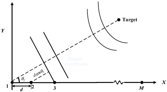
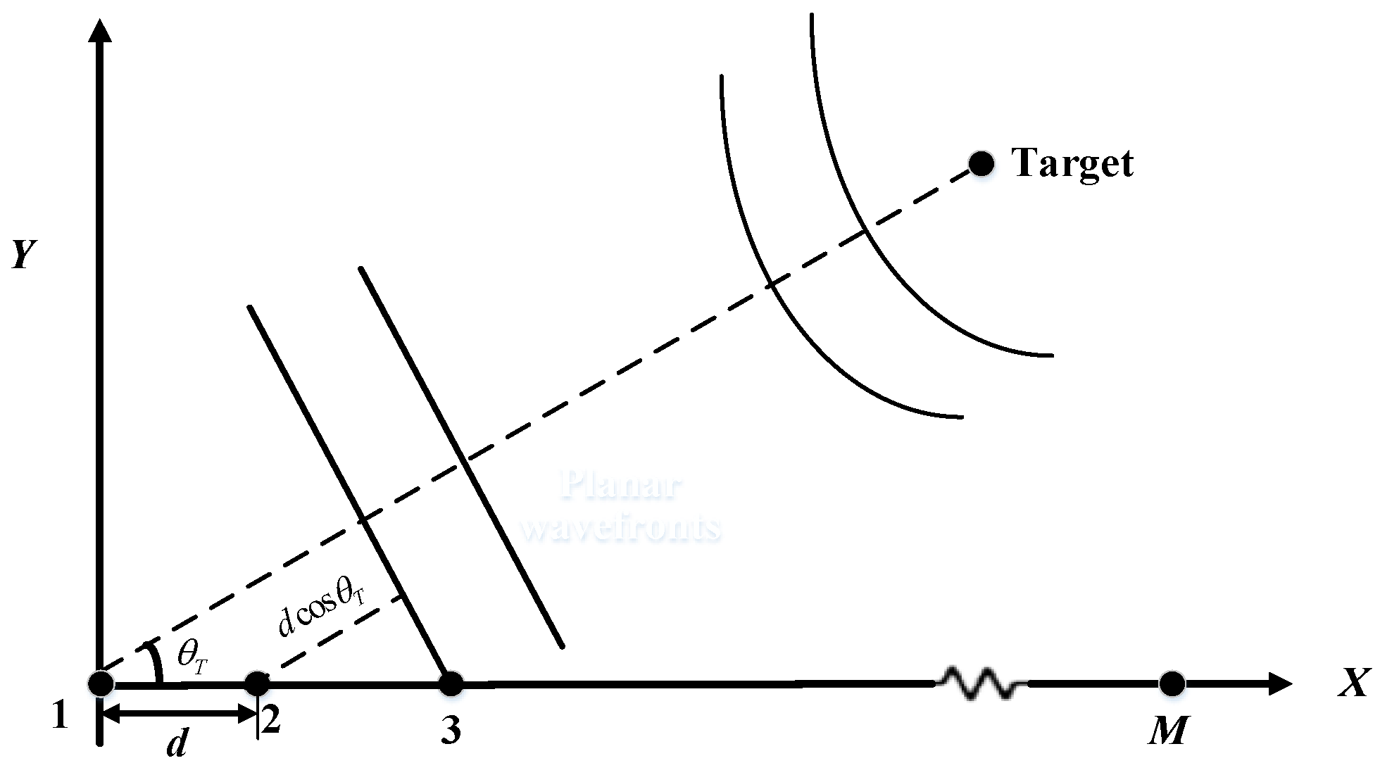
In this paper, a uniform linear array is considered, composed of M omnidirectional sensors uniformly spaced with a separation distance d, as illustrated in Figure 1. The source is assumed to be a narrow-band point source located in the far-field of the array. Physically, the far-field assumption implies that the radius of curvature of the wavefront is large enough to be considered negligible across the array aperture. Consequently, the wavefronts impinging on the sensors are modeled as plane waves, and the signal rays arriving at the array are parallel to each other. Additionally, the background noise is modeled as spatially white Gaussian noise, which is uncorrelated with the source signal.

Figure 1. ULA with signal impinging from direction θ_T.

Under this plane-wave assumption, the geometric relationship between the signal direction and the array structure becomes linear. As shown in Figure 1, for a signal impinging from a direction ${\theta }_T$, the wavefront arrives at the mth sensor later than the (m − 1)th sensor due to the additional propagation path. This spatial path difference, given by $\mathrm{\Delta }r=d\cos {\theta }_T$, directly translates into a temporal delay $\tau$ determined by the speed of sound propagation c. This mechanism forms the physical basis for spatial filtering, allowing the array to discriminate signals based on their arrival angles.

According to [20,21], the narrow-band far-field signal model is adopted, which effectively captures the phase relationships of distant targets, distinct from near-field models that require wavefront curvature parameters or wideband models that necessitate frequency decomposition.

Using the first sensor as the reference, the time delay between the mth sensor and the reference sensor can be denoted as

$${\tau }_m\left({\theta }_T\right)={\displaystyle \frac{\left(m-1\right)d\cos {\theta }_T}{c}}$$

(1)

where c is the speed of sound propagation in the sea. Here, the explicit time-domain formulation is adopted to provide a straightforward physical interpretation of the propagation time delay across the array aperture. Furthermore, this real-valued representation aligns with the physical reality that hydrophones in practical sonar systems inherently capture real-valued signals. Assuming that the received narrowband signal by the reference sensor is written as

$$s\left(t\right)=A\cos \left(2\pi f_{0}t\right)$$

(2)

The observed signal received by the mth sensor can be expressed as

$$x_m\left(t\right)=A\cos \left\{2\pi f_0\left[t+{\displaystyle \frac{\left(m-1\right)d\cos {\theta }_T}{c}}\right]\right\}+w_m\left(t\right)$$

(3)

where f₀ is the frequency of the narrow-band source and w_m(t) is the additive Gaussian white noise with zero-mean and variance ${\sigma }_n^2$ on the mth sensor. Furthermore, w_m(t) is uncorrelated from one sensor to another and also uncorrelated with the signal.

Based on the propagation delay model established in Equation (1), CBF performs spatial filtering through a “delay-and-sum” mechanism. To estimate the source DOA, the CBF coherently combines the observed signals $x_m\left(t\right)$ (given in Equation (3)) by compensating for the relative time delays associated with a scanning angle $\theta$. By aligning and summing the sensor outputs, the preformed beam output is derived as

$$\begin{array}{cc}y(t,\theta )& ={\displaystyle \frac{1}{M}}{\displaystyle \sum _{m=1}^M{s}_m\left[t+{\tau }_m\left(\theta \right)\right]}\hfill \\ & =A\cos \left[2\pi f_{0}t+{\displaystyle \frac{\left(M-1\right)\phi \left(\theta \right)}{2}}\right]{\displaystyle \frac{\sin \left[M\phi \left(\theta \right)\right]}{M\sin \left[\phi \left(\theta \right)\right]}}\hfill \end{array}$$

(4)

where $\phi \left(\theta \right)=\pi d\left(\cos {\theta }_T-\cos \theta \right)/\lambda$ and $\lambda =c/f_0$. The beam power as a function of the steering angle is given by

$$P\left(\theta \right)={\displaystyle \int y^2\left(t,\theta \right)}\mathrm{d}t={\displaystyle \frac{A^2}{2}}{\left\{{\displaystyle \frac{\sin \left[M\phi \left(\theta \right)\right]}{M\sin \left[\phi \left(\theta \right)\right]}}\right\}}^2={\displaystyle \frac{A^2}{2}}{\left[D\left(\theta \right)\right]}^2$$

(5)

where D(θ) is the beam pattern. It is given by

$$D\left(\theta \right)=\left|{\displaystyle \frac{\sin \left[M\phi \left(\theta \right)\right]}{M\sin \left[\phi \left(\theta \right)\right]}}\right|$$

(6)

Equations (5) and (6) show that the maximum value occurs at θ = θ_T, hence the peak of the beam power can be used to estimate the DOA of a given target, i.e.,

$${\widehat{\theta }}_T=\arg \underset{\theta }{\max }P\left(\theta \right)$$

(7)

When there exists noise and the steering angle coincides with the DOA of a given target, the target signals are coherently summed. However, noise is uncorrelated between the receivers (spaced at half-wavelength) and is hence incoherently summed. Consequently, the SNR at the output of beamforming is enhanced compared with the input SNR. The SNR gain is

$$G_s={\displaystyle \frac{{\sigma }_s^2}{{\sigma }_n^2/M}}/{\displaystyle \frac{{\sigma }_s^2}{{\sigma }_n^2}}=M$$

(8)

The realization of this maximum array gain M is contingent upon two fundamental conditions: the background noise must be spatially uncorrelated (white), and the beamformer’s steering direction must coincide exactly with the true direction of arrival.

2.2. Determination of the Preformed Steering Beams

Equation (7) indicates that, for high SNRs, the DOA of the target can be precisely estimated theoretically when the steering $\theta$ takes any continuous value in the range of 0°~180°. However, only a finite number of steering angles can be employed in practical applications. It is important to clarify that while the Rayleigh limit strictly pertains to the separability of multiple sources (resolution), the broad main lobe associated with the array aperture poses challenges for precise peak localization in single-source estimation. Therefore, for DOA estimation via CBF, a primary task is to determine the optimal number and distribution of preformed beams. When designing beamformers for linear arrays, it is common practice to steer beams uniformly spaced in cosine space ($\cos \theta$). At the half-wavelength frequency, these beams are independent and overlap at their nominal 3 dB points [22].

Next, the beamwidth of a ULA is analyzed. It is defined as the angular distance between the −3 dB (0.707) points of D(θ). To avoid spatial aliasing, d/λ is restricted to be less than 0.5, i.e., d < λ_min/2 [23]. To facilitate the analysis, this derivation employs a second-order Taylor expansion around the peak. The resulting asymptotic approximation is valid under the condition of a sufficiently large number of sensors and implies that the angular deviation from the main lobe peak is small. Under these assumptions, the beam power function in Equation (6) can be asymptotically approximated as

$$D\left(\theta \right)=\left|{\displaystyle \frac{\sin \left[M\phi \left(\theta \right)\right]}{M\phi \left(\theta \right)}}\right|$$

(9)

For $\sin x/x=0.707$ when x = 1.39, the interval cosine value corresponding to two adjacent steering beams is $1.39\lambda /\pi Md$. Assume that the number of ‘preformed’ beams needed, denoted as K, is determined by the beamwidth of an unshaded beam in cosθ space. Since cos(0°) = 1 and cos(180°) = −1, this yields

$${\mathrm{\Delta }}_C={\displaystyle \frac{2}{K-1}}={\displaystyle \frac{2.78\lambda }{\pi Md}}$$

(10)

From Equation (10), the expression is derived as

$$K={\displaystyle \frac{\pi Md}{1.39\lambda }}+1$$

(11)

For d < λ_min/2, it follows that

$$K_{\min }={\displaystyle \frac{\pi M}{2.78}}+1$$

(12)

Substituting Equation (12) into Equation (10) yields

$${\mathrm{\Delta }}_{C_{\min }}={\displaystyle \frac{2}{K_{\min }-1}}={\displaystyle \frac{2}{\pi M/2.78+1-1}}={\displaystyle \frac{5.56}{\pi M}}$$

(13)

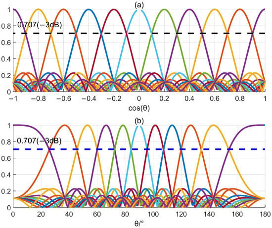
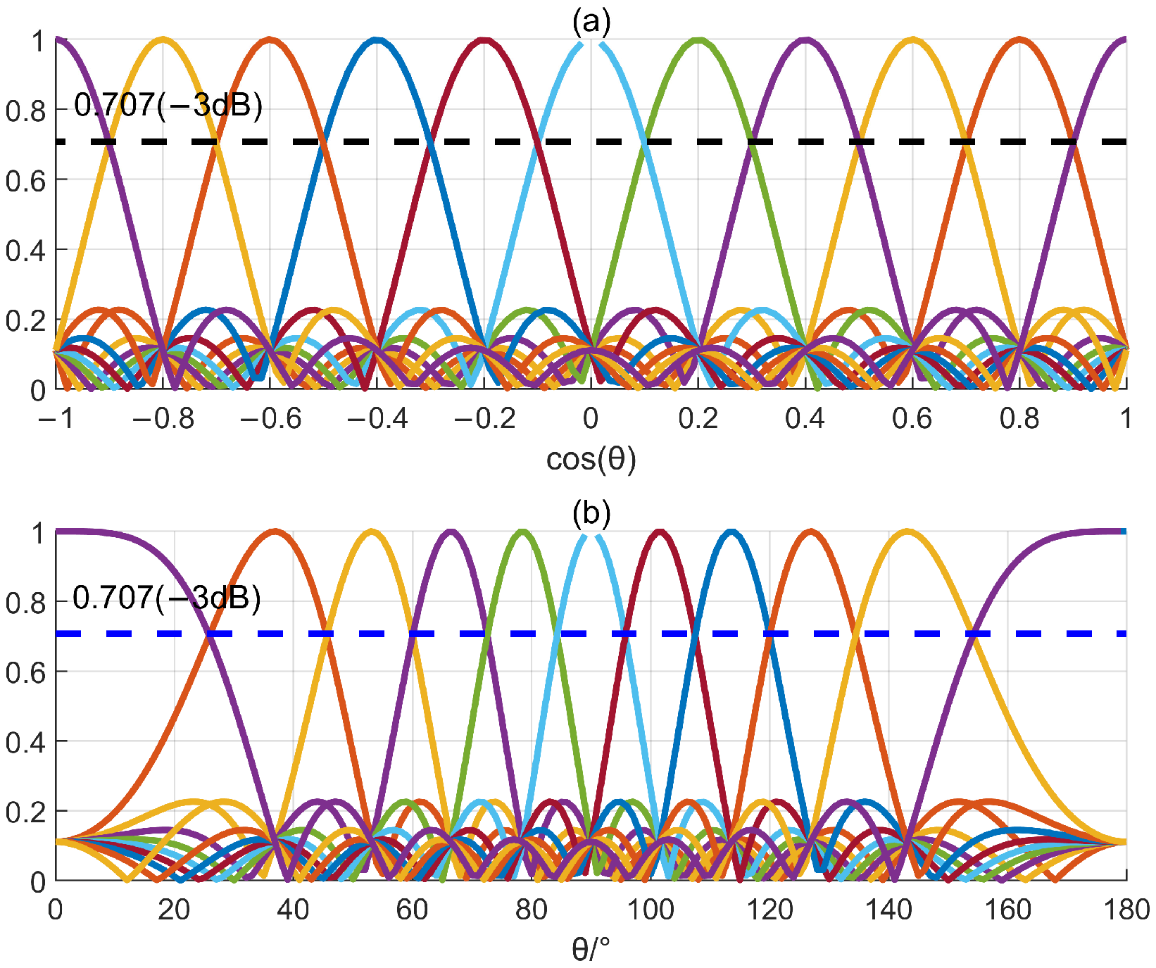
This is illustrated in Figure 2, where different colored curves represent individual beams steered to distinct directions. Specifically, Figure 2a depicts the beam patterns in the cosine domain ($u=\cos \theta$), characterized by uniform spacing and constant beamwidth, with crossover points at −3 dB. In contrast, Figure 2b shows the corresponding patterns in the angular domain ($\theta$), clearly demonstrating the non-uniform spacing and significant beam broadening near the endfire directions. This phenomenon arises because spatial sampling is inherently uniform in the u-domain; however, the mapping to the $\theta$-domain introduces a nonlinear distortion. Consequently, the angular resolution becomes non-uniform, widening significantly as the direction approaches the endfire. The preformed steering beam directions, or Maximum Response Axes (MRAs), are determined by

$$\cos {\theta }_k=1-\left(k-1\right){\mathrm{\Delta }}_{c_{\min }}=1-{\displaystyle \frac{2\left(k-1\right)}{K_{\min }-1}},k=1,2,\dots ,K_{\min }$$

(14)

Figure 2. Beam pattern set spanning all angular space (d = λ/2). (a) Cosine domain; (b) Angular domain.

In this paper, unless otherwise stated, the number of preformed steering beams and directions are set, respectively, as given by Equations (12) and (13) for the ULA.

3. Proposed DOA Estimation Method

In this section, the MSA estimator is introduced to address the precision limitations of the Conventional Beamformer. The core innovation of the MSA estimator is to treat the DOA estimation as an inverse problem based on the exact theoretical beam pattern of the ULA. Unlike the PIA estimator, which approximates the main lobe using a polynomial and inherently suffers from model mismatch, the MSA estimator employs the Bisection Method to numerically solve for the exact fractional DOA offset. By iteratively narrowing down the search interval based on the monotonic relationship between the beam power ratio and the direction deviation, the bisection method ensures convergence to the precise solution without the need for derivative calculations. This approach effectively eliminates model mismatch errors, offering superior robustness and estimation accuracy compared to conventional interpolation methods.

3.1. Proposed DOA Estimation Method for ULA

From Equation (14), the DOA θ_T can be written as

$$\cos {\theta }_T=1-\left(k_p-1+\delta \right){\mathrm{\Delta }}_{C_{\min }}$$

(15)

where k_p denotes the index corresponding to the peak of the discrete CBF power spectrum, and δ is a fractional correction term in the interval [−0.5, 0.5]. In the absence of noise, substituting $\cos {\mathrm{\theta }}_T=1-\left(k_p-1+\delta \right){\mathrm{\Delta }}_C$ and $\cos {\theta }_{k_p}=1-\left(k_p-1\right){\mathrm{\Delta }}_C$ into Equation (9) yields

$$D\left({\theta }_{k_p}\right)=\left|{\displaystyle \frac{\sin \left(\frac{M\pi d\delta }{\lambda }{\mathrm{\Delta }}_{C_{\min }}\right)}{M\sin \left(\frac{\pi d\delta }{\lambda }{\mathrm{\Delta }}_{C_{\min }}\right)}}\right|\approx \left|{\displaystyle \frac{\sin \left(\frac{M\pi d\delta }{\lambda }{\mathrm{\Delta }}_{C_{\min }}\right)}{M\frac{\pi d\delta }{\lambda }{\mathrm{\Delta }}_{C_{\min }}}}\right|$$

(16)

Substituting Equation (13) into Equation (16), the following is obtained:

$$D\left({\theta }_{k_p}\right)\approx \left|{\displaystyle \frac{\sin \left(5.56\xi \delta \right)}{5.56\xi \delta }}\right|$$

(17)

where $\xi =d/\lambda$. Similarly, it can be derived that

$$D\left({\theta }_{k_p-1}\right)\approx \left|{\displaystyle \frac{\sin \left[5.56\xi \left(1+\delta \right)\right]}{5.56\xi \left(1+\delta \right)}}\right|$$

(18)

$$D\left({\theta }_{k_p+1}\right)\approx \left|{\displaystyle \frac{\sin \left[5.56\xi \left(1-\delta \right)\right]}{5.56\xi \left(1-\delta \right)}}\right|$$

(19)

From Equation (17), it can be seen that $D\left({\theta }_{k_p}\right)$ is given by sinc(x) = sin(x)/x. Expanding sinc(x) by the Taylor series yields

$${\displaystyle \frac{\sin x}{x}}=1-x^2/3!+x^4/5!-\dots +{\left(-1\right)}^{k-1}{x}^{2k-2}/\left(2k-1\right)!$$

(20)

Since the coarse search index k_p locates the immediate vicinity of the true peak, the argument x corresponds to a small angular offset. Under this condition the higher-order terms in the Taylor series are negligible. Consequently, Equation (20) can be approximated as

$${\displaystyle \frac{\sin x}{x}}\approx 1-{\displaystyle \frac{x^2}{6}}$$

(21)

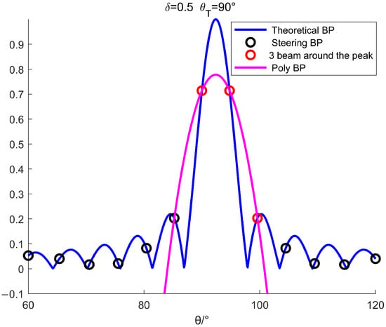
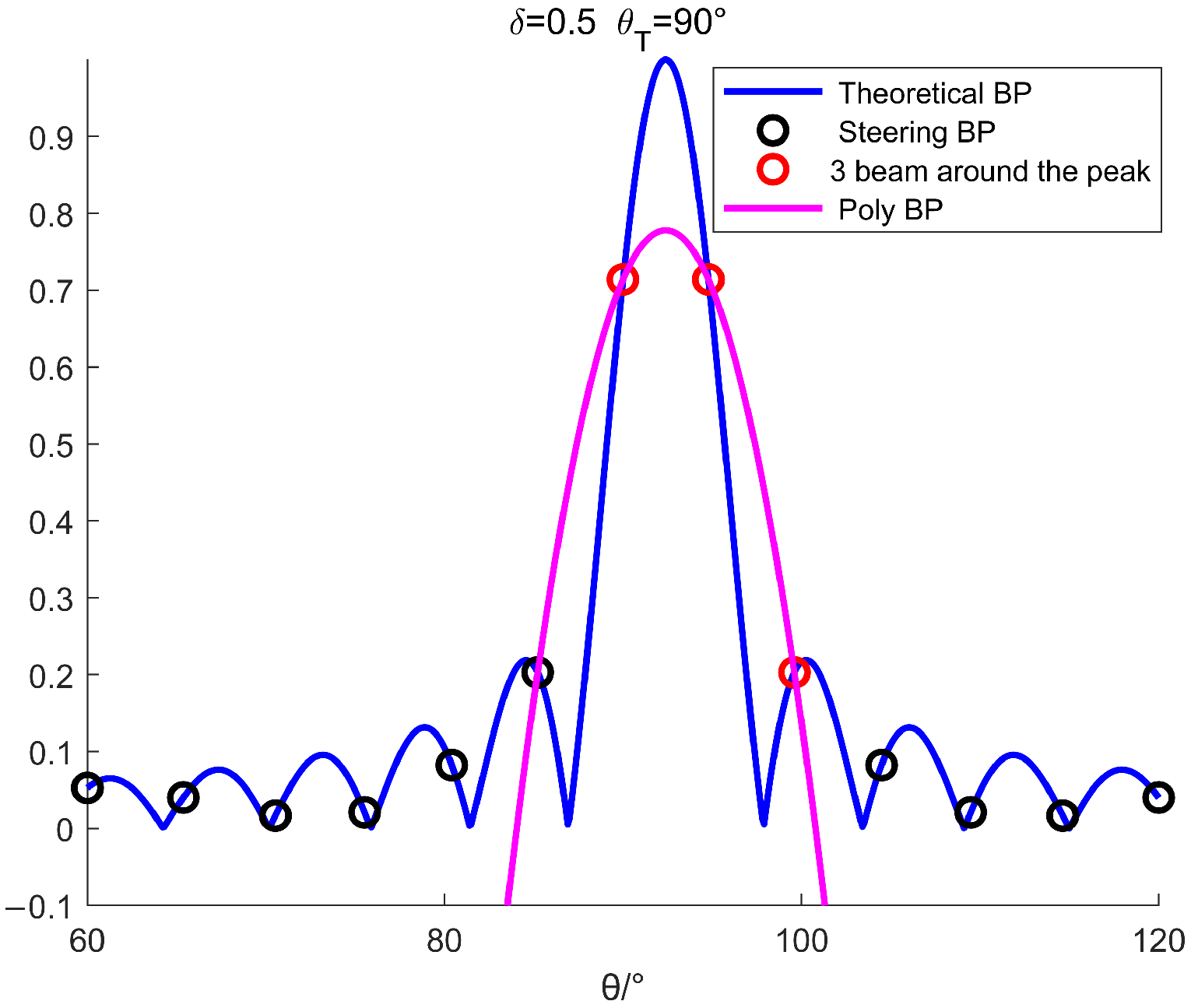
As shown in Equation (21), the beam pattern of the ULA can be approximately seen as a parabola near the main lobe. Therefore, by leveraging three samples around the peak of the main lobe, the DOA of the target can be estimated by searching the maximum point of the fitting parabola. Parabola fitting for the main lobe of the beam pattern is illustrated in Figure 3. Physically, a fundamental distinction exists between the two curves shown. The actual beam pattern is governed by the physics of wave propagation and the array manifold, typically following a Dirichlet kernel (sinc-like) function. In contrast, the PIA estimator attempts to approximate this transcendental shape using a simple second-order polynomial. From Figure 3, it is evident that while the fitting parabola approaches the main lobe, it does not perfectly match the true beam shape, resulting in a deviation between their maximum points. This visual discrepancy represents the inherent model mismatch error. Since the physical beam pattern is not strictly parabolic, this approximation introduces a systematic bias into the DOA estimation, particularly when the target is located midway between grid points.

Figure 3. Parabola fitting for the main lobe of the beam pattern (BP) (δ = 0.5).

The parabolic equation is given by

$$y=a{x}^2+bx+c$$

(22)

For the sake of brevity, we denote

$$V_{-1}=D\left({\theta }_{k_p-1}\right),V_0=D\left({\theta }_{k_p}\right),V_1=D\left({\theta }_{k_p+1}\right)$$

(23)

Substituting $\left({\theta }_{k_p-1},V_{-1}\right),\left({\theta }_{k_p},V_0\right),\left({\theta }_{k_p+1},V_1\right)$ into Equation (22), it follows that

$$\cos {\widehat{\theta }}_T=-{\displaystyle \frac{b}{2a}}={\displaystyle \frac{V_{-1}-2V_0+V_1}{2\left(4V_0-V_{-1}-3V_1-4k_p{V}_0+2k_p{V}_{-1}+2k_p{V}_1\right){\mathrm{\Delta }}_C-8V_0+4V_{-1}+4V_1}}$$

(24)

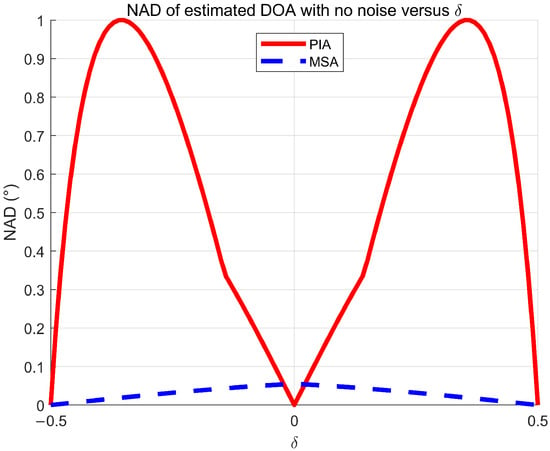
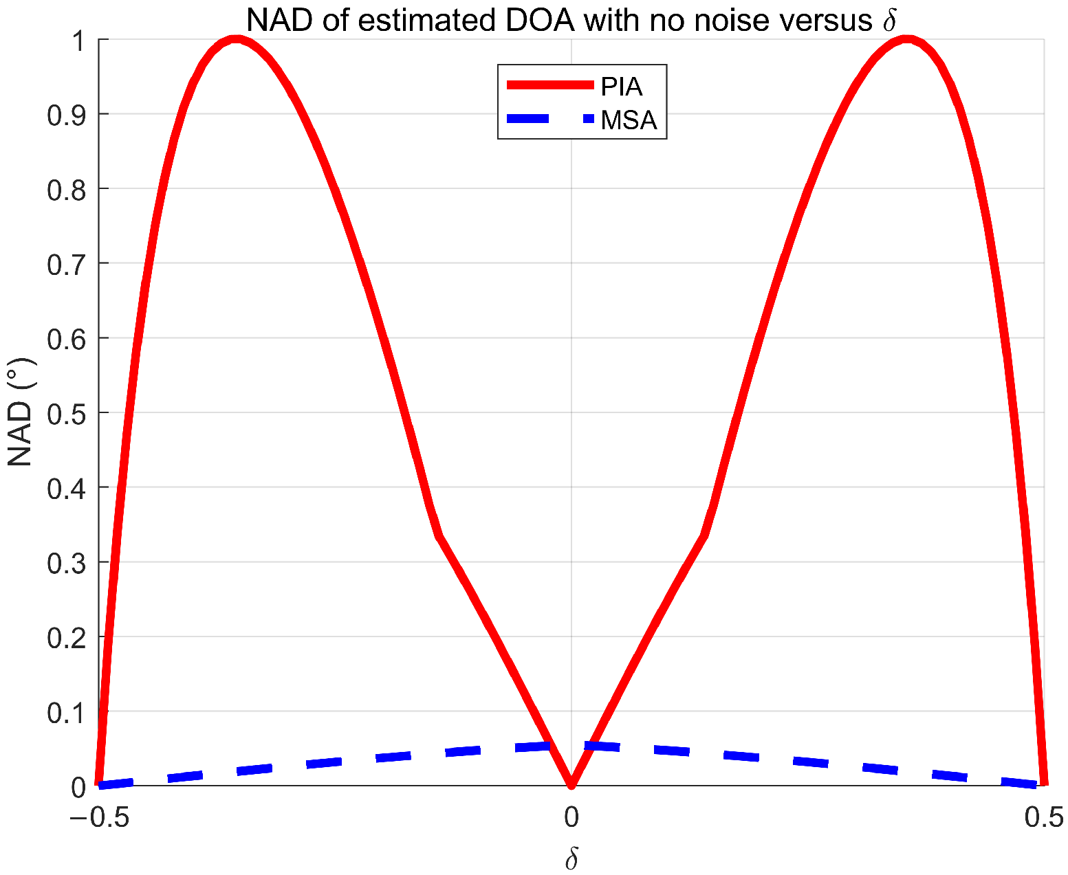
The DOA ${\widehat{\theta }}_T$ estimated by Equation (24) was proposed by Qihu Li and it is denoted as the PIA estimator [18]. The normalized absolute deviation (NAD) of estimated DOA with no noise versus δ is shown by the red solid line in Figure 4. Due to the simplicity of the PIA estimator, it has been widely used in practical applications. However, as observed in Figure 4, the accuracy of the PIA estimator is highly sensitive to the relative direction deviation δ. The NAD increases significantly as the magnitude of deviation $\left|\delta \right|$ increases. This degradation is caused by the model mismatch between the approximate parabola and the actual main lobe shape, which becomes more severe at larger deviations. In contrast, the proposed MSA estimator maintains an error level orders of magnitude lower than the PIA estimator across the deviation range. This significant performance gap demonstrates the theoretical advantage of the proposed model solution approach, as the MSA estimator is limited only by numerical tolerance, whereas the PIA estimator suffers from systematic bias.

Figure 4. NAD of estimated DOA versus δ with no noise.

To solve this problem, the MSA estimator is proposed using the theoretical beam pattern of the given ULA to estimate the DOA. Assume that the k_pth steering beam is the maximal one among $P\left({\theta }_k\right),k=1,2,\cdots ,K_{\min }$, i.e.,

$$k_p=\arg \underset{k=1,2,\cdots ,K_{\min }}{\max }P\left({\theta }_k\right)$$

(25)

It is assumed that a coarse search returns the index of the true maximum bin k_p. The estimated DOA is then given by

$${\widehat{\theta }}_T=\mathrm{a}\cos \left[1-\left(k_p-1+\widehat{\delta }\right){\mathrm{\Delta }}_C\right]$$

(26)

Thus our goal is to estimate the fractional correction term δ. Denote $A_1=D\left({\theta }_{k_p}\right)$ and $A_2=\max \left(D\left({\theta }_{k_p-1}\right),D\left({\theta }_{k_p+1}\right)\right)$, it can be derived that

$$A_1=\left|{\displaystyle \frac{\sin \left(5.56\xi \delta \right)}{5.56\xi \delta }}\right|,A_2=\left|{\displaystyle \frac{\sin \left[5.56\xi (1-\left|\delta \right|)\right]}{5.56\xi (1-\left|\delta \right|)}}\right|$$

(27)

Denote $A_2/A_1$ as $\alpha$, from Equation (27), the following is obtained:

$$\alpha \left(\left|\delta \right|\right)={\displaystyle \frac{A_2}{A_1}}={\displaystyle \frac{\left|\delta \right|}{1-\left|\delta \right|}}\left|{\displaystyle \frac{\sin \left[5.56\xi (1-\left|\delta \right|)\right]}{\sin \left(5.56\xi \left|\delta \right|\right)}}\right|$$

(28)

It is evident that the analytical solutions cannot be obtained from the nonlinear Equation (28). The numerical solution method can be used to solve the nonlinear equation. To estimate the DOA by a numerical solution method, it must first be established that there exists a unique solution for the nonlinear equation. By investigation of Equation (28), $\alpha \left(\left|\delta \right|\right)$ increases monotonically, with the $\left|\delta \right|$ varying from 0 to 0.5. Therefore, it satisfies that there exists a unique solution. Secondly, it needs to satisfy that there exists a fast solution algorithm. For $\left|\delta \right|$ varying from 0 to 0.5, which is a very small region, the bisection method can be used to solve the nonlinear Equation (28) [22]. For the observed signal with noise,

$$\widehat{\alpha }\left(\left|\widehat{\delta }\right|\right)={\displaystyle \frac{\max \left(\sqrt{P\left({\theta }_{k_p-1}\right)},\sqrt{P\left({\theta }_{k_p+1}\right)}\right)}{\sqrt{P\left({\theta }_{k_p}\right)}}}={\displaystyle \frac{\left|\widehat{\delta }\right|}{1-\left|\widehat{\delta }\right|}}\left|{\displaystyle \frac{\sin \left[5.56\xi (1-\left|\widehat{\delta }\right|)\right]}{\sin \left(5.56\xi \left|\widehat{\delta }\right|\right)}}\right|$$

(29)

The proposed MSA estimator estimates $\left|\widehat{\delta }\right|$ by numerical solution for Equation (29) using the bisection method. Then the estimated DOA can be given by

$${\widehat{\theta }}_T=\left\{\begin{array}{cc}\mathrm{acos}\left[1-\left(k_p-1+\left|\widehat{\delta }\right|\right){\mathrm{\Delta }}_C\right]& \sqrt{P\left({\theta }_{k_p-1}\right)}<\sqrt{P\left({\theta }_{k_p+1}\right)}\\ \mathrm{acos}\left[1-\left(k_p-1-\left|\widehat{\delta }\right|\right){\mathrm{\Delta }}_C\right]& \sqrt{P\left({\theta }_{k_p-1}\right)}\ge \sqrt{P\left({\theta }_{k_p+1}\right)}\end{array}\right.$$

(30)

The main procedures of the proposed MSA estimator are as follows:

Step 1: Search the peak steering beam k_p by Equation (25);

Step 2: Compute the ratio of the peak value and the adjacent submaximal component in the main lobe:

$$\widehat{\alpha }\left(\left|\widehat{\delta }\right|\right)={\displaystyle \frac{\max \left(\sqrt{P\left({\theta }_{k_p-1}\right)},\sqrt{P\left({\theta }_{k_p+1}\right)}\right)}{\sqrt{P\left({\theta }_{k_p}\right)}}}$$

(31)

Step 3: Initialization: initialize the lower and upper bounds of the interval for bisection method, a₀ = 0 and b₀ = 0.5; set the iterative number of times q = 0 and set the bisection accuracy ε, then the number of bisections N_B is given as

$$N_B=⌈{\log }_2\left({\displaystyle \frac{b_0-a_0}{\epsilon }}\right)⌉$$

(32)

where $\lceil \rceil$ denotes the rounding up operator. In this paper, ε is set to 0.00001, therefore N_B = 16.

Step 4: Iteratively using the bisection method:

(1) Calculating the value of Equation (28) for the midpoint yields $\alpha \left({\displaystyle \frac{a_0+b_0}{2}}\right)$;

(2) Decide which side to go, and replace either the lower or upper bound with the midpoint to cut the region in half:

If $\alpha \left({\displaystyle \frac{a_0+b_0}{2}}\right)>\widehat{\alpha }$, set $a_0=a_0$ and $b_0={\displaystyle \frac{a_0+b_0}{2}}$; else set $a_0={\displaystyle \frac{a_0+b_0}{2}}$ and $b_0=b_0$;

(3) Set q = q + 1, repeat step 4 until q = N_B.

Step 5: Setting $\left|\widehat{\delta }\right|=\left(a_0+b_0\right)/2$ and submitting it into Equation (30) yields the estimated DOA ${\widehat{\theta }}_T$.

As shown by the blue dotted line in Figure 4, the proposed MSA estimator is much more robust against the |δ| than the PIA estimator. This is because the theoretical main lobe model is directly used to estimate the DOA by the MSA estimator, and there exists no model mismatch compared with the PIA estimator.

3.2. Generalization to Arrays with Arbitrary Geometries

Although the MSA estimator is proposed for the ULA by numerical solution of Equation (29), it can be generalized to arrays with arbitrary geometries. From Equation (29), it is evident that the core stage to generalize the MSA estimator for arrays with arbitrary geometries is to obtain the theoretical beam pattern. Next, the general expression of the theoretical beam pattern for arrays with arbitrary geometries is analyzed.

In the absence of noise, for a far-field narrow-band source with frequency f₀ and DOA θ_T, the preformed beam with the steering direction θ can be expressed as follows:

$$y\left(t,\theta \right)={\displaystyle \frac{1}{M}}{\displaystyle \sum _{m=1}^{M}A\cos \left\{2\pi f_0\left[t+{\mathrm{\Delta }}_m\left(\theta ,{\theta }_T\right)\right]\right\}}$$

(33)

where ${\mathrm{\Delta }}_m\left(\theta ,{\theta }_T\right)={\tau }_m\left(\theta \right)-{\tau }_m\left({\theta }_T\right)$ and ${\tau }_m\left(\theta \right)$ are the relative time delays between the mth sensor and the reference one. The theoretical beam pattern as a function of the steering angle is then given by

$$\begin{array}{cc}{D}_{\mathrm{A}}\left(\theta ,{\theta }_T\right)& ={\displaystyle \frac{1}{M}}{\left\{E\left[y^2\left(t,\theta \right)\right]\right\}}^{1/2}\hfill \\ & ={\displaystyle \frac{1}{2}}{\left\{{\left[{\displaystyle \sum _{m=1}^M\cos \left(2\pi f{\mathrm{\Delta }}_m\left(\theta \right)\right)}\right]}^2+{\left[{\displaystyle \sum _{m=1}^M\sin \left(2\pi f{\mathrm{\Delta }}_m\left(\theta \right)\right)}\right]}^2\right\}}^{1/2}\end{array}$$

(34)

The subscript A indicates arrays with arbitrary geometries; it is used to make a distinction from the ULA. The beam power as a function of the steering angle is given by

$$P_{\mathrm{A}}\left(\theta \right)={\displaystyle \frac{1}{T}}{\displaystyle {\int }_0^T{y}^2\left(t,\theta \right)\mathrm{d}t}$$

(35)

From Equations (34) and (35), it follows that

$${\widehat{\alpha }}_{\mathrm{A}}\left({\widehat{\theta }}_T\right)={\displaystyle \frac{\max \left(\sqrt{P_{\mathrm{A}}\left({\theta }_{k_p-1}\right)},\sqrt{P_{\mathrm{A}}\left({\theta }_{k_p+1}\right)}\right)}{\sqrt{P_{\mathrm{A}}\left({\theta }_{k_p}\right)}}}$$

(36)

Unlike the MSA estimator for the ULA, the generalized MSA (GMSA) estimator directly solves the DOA ${\widehat{\theta }}_T$ instead of $\left|\widehat{\delta }\right|$. When $\sqrt{P_{\mathrm{A}}\left({\theta }_{k_p-1}\right)}>\sqrt{P_{\mathrm{A}}\left({\theta }_{k_p+1}\right)}$, ${\widehat{\theta }}_T$ is solved by the bisection method in the interval of [${\theta }_{k_p-1}$,${\theta }_{k_p}$]. When $\sqrt{P_{\mathrm{A}}\left({\theta }_{k_p-1}\right)}<\sqrt{P_{\mathrm{A}}\left({\theta }_{k_p+1}\right)}$, ${\widehat{\theta }}_T$ is solved by the bisection method from ${\theta }_{k_p}$ to ${\theta }_{k_p+1}$.

4. Simulations

In this section, the performance comparison for the proposed MSA estimator is carried out with the existing state-of-the-art methods, including the PIA estimator via CBF and a high-resolution MUSIC estimator, by Monte Carlo simulations. The performance of the proposed DOA estimator is assessed using the root mean square error (RMSE) as a performance measure. The RMSE is computed for each estimator as follows:

$$\mathrm{RMSE}\left({\widehat{\theta }}_T\right)=\sqrt{{\displaystyle \frac{1}{M_C}}{\displaystyle \sum _{q=1}^{M_c}{\left({\widehat{\theta }}_T^{\left(q\right)}-{\theta }_T\right)}^2}}$$

(37)

where M_C is the number of Monte Carlo simulations, which is set to M_C = 1000 in all simulations, and ${\widehat{\theta }}_T^{\left(q\right)}$ is the estimate of ${\theta }_T$ from the qth Monte-Carlo run. The well-known Cramér-Rao lower bound (CRLB) is also considered as a benchmark against which the performance of the proposed method is compared [23]. The CRLB of the DOA estimation for a far-field narrowband signal received by the ULA is given as [21]

$$\mathrm{var}\left({\widehat{\theta }}_T\right)\ge {\displaystyle \frac{3\left(M-1\right)c^2}{{\pi }^2\eta M\left(M+1\right)L^2{f}_0^2{\sin }^2{\theta }_T}}$$

(38)

where $\eta =A^2/\left(2{\sigma }_n^2\right)$, and L = (M − l)d is the length of the array. Note that it is easiest to estimate the bearing if θ_T = 90° and impossible if θ_T = 0°. Furthermore, the bound depends critically on the array length in wavelengths or L/λ, as well as on the SNR at the array output, or Mη.

The signals are generated according to the signal model given by Equation (3). The sampling frequency is set to 4 kHz. For the ULA, the array parameters are configured to align with the hardware specifications utilized in our actual underwater acoustic experiments. Specifically, the sensor number M is set to 21, and the spacing d is set to 0.6 m, which corresponds to a half-wavelength with f₀ = 1250 Hz. From Equation (12), it is easy to see that the number of preformed steering beams K is 25. Then, the directions of the preformed steering beams are given by Equation (14), and they are {0, 23.56, 33.56, 41.41, 48.19, 54.31, 60, 65.38, 70.53, 75.52, 80.4, 85.22, 90, 94.78, 99.6, 104.48, 109.47, 114.62, 120, 125.69, 131.81, 138.59, 146.44, 156.44, 180} in degrees. For the MUSIC estimator, the steering directions are set to start from 0° to 180° in steps of 0.001°.

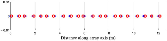
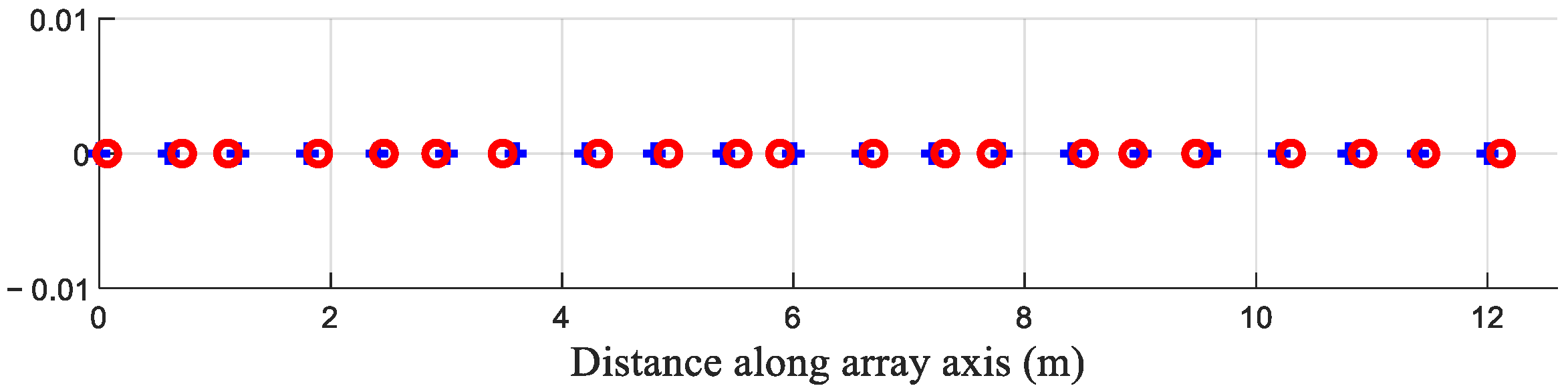
In array beamforming, the signal model usually assumes plane wave arrivals for distant sources. This model is often incorrect due to signal scattering from the random medium or incorrectly assumed source positions. The signal mismatch can cause wider beamwidths, higher sidelobes, and even the disappearance of the signal, as in high-resolution adaptive beamforming. How sensitive the DOA estimation accuracy is to signal mismatch is an important performance measure for a DOA estimator. Since signal mismatch is due to signal amplitude and phase errors, array performance degradation can be simulated by emulating signal mismatch with random position errors for the receivers [14]. As an example, a ULA with position errors is shown in Figure 5. The actual receiver positions are denoted by red circles “o” in Figure 5, as opposed to a ULA with receivers denoted by blue crosses “+”. When analyzing the sensitivity to the Position Errors (PE) for the DOA estimator, it is assumed that a random position error follows a uniform distribution from 0 to 0.15 d for each sensor, which is high for an actual position error. Furthermore, these errors are treated as unknown, and one carries out beamforming assuming a uniform line array.

Figure 5. View of the ULA configuration.

Three cases are presented and discussed in this section, including the RMSE of ${\widehat{\theta }}_T$ versus δs, the RMSE of ${\widehat{\theta }}_T$ versus SNRs, and the RMSE of ${\widehat{\theta }}_T$ versus different frequencies f₀. For each presented case, simulations with both position and no position errors are given. Finally, the computational complexity of the algorithms is analyzed, and their DOA estimation performance is demonstrated in the context of a non-uniform linear array (NULA).

4.1. Case 1: RMSE of ${\widehat{\theta }}_T$ Versus δs

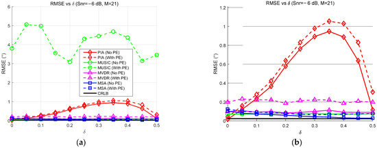
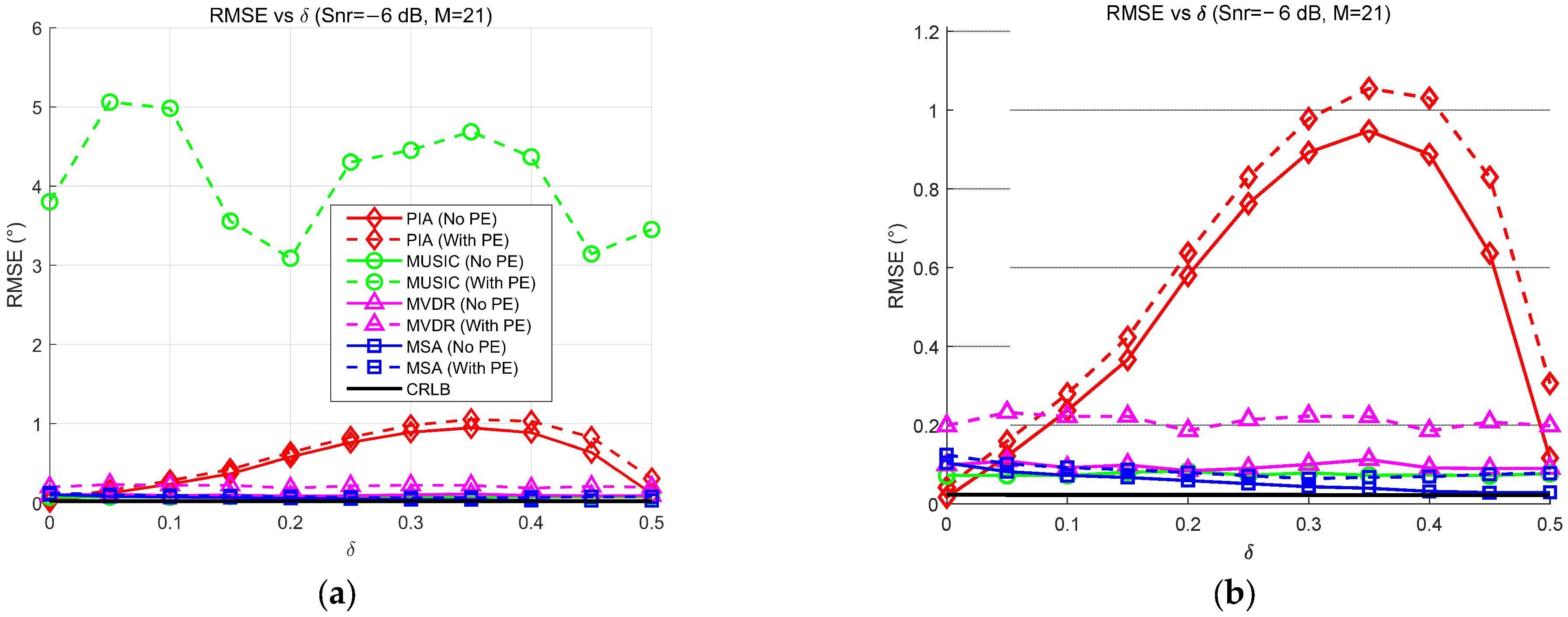
Firstly, the performance of the estimators is evaluated by plotting the Root Mean Square Error (RMSE) of ${\widehat{\theta }}_T$ versus the fractional correction term $\delta$. The simulation setup fixes the SNR at −6 dB, varies $\delta$ from 0 to 0.5, and sets the peak steering beam index $k_p$ to 5 (corresponding to 48.19°). Figure 6a presents the global view to capture the overall stability, while Figure 6b offers a magnified view to analyze the estimation precision.

Figure 6. RMSE of ${\widehat{\theta }}_T$ versus δs with SNR = −6 dB. (a) Original figure; (b) zoomed-in view of (a).

From the global trend in Figure 6a, a clear distinction in robustness is observed. The MUSIC estimator (green) exhibits severe instability in the presence of sensor position errors. As $\delta$ increases, its RMSE fluctuates violently, exhibiting catastrophic spikes (e.g., exceeding 3.8°) that indicate a complete failure to resolve the target. In contrast, the PIA estimator (marked with red diamonds) exhibits a convex error profile. Its RMSE rises from a baseline of ~0.2° to a peak of ~1.1° at intermediate offsets ($\delta \approx 0.35$), before decreasing as $\delta$ approaches 0.5 due to the structural symmetry of the beam pattern. Despite this drop at the midpoint, the substantial errors at intermediate deviations clearly highlight the severe model mismatch of the PIA estimator compared to the stable accuracy of the proposed MSA estimator. The MVDR estimator (marked with magenta triangles), on the other hand, maintains a stable performance profile similar to the proposed method, unaffected by the variation of $\delta$, but it comes at the cost of high computational complexity due to matrix inversion.

Conversely, the magnified view in Figure 6b highlights the superior accuracy of the proposed method. The MSA estimator (blue squares) maintains a consistently flat error profile across the entire range of $\delta$. Even under position errors (blue dashed line), the RMSE of the MSA estimator stabilizes around 0.12°, closely tracking the theoretical Cramér-Rao Lower Bound (CRLB). While the MVDR estimator is also robust, it exhibits a slightly higher baseline error of approximately 0.15°. This comparison demonstrates that the proposed MSA estimator effectively eliminates the model mismatch bias inherent to the PIA estimator and achieves higher precision than the MVDR without the heavy computational burden.

4.2. Case 2: RMSE of ${\widehat{\theta }}_T$ Versus SNRs

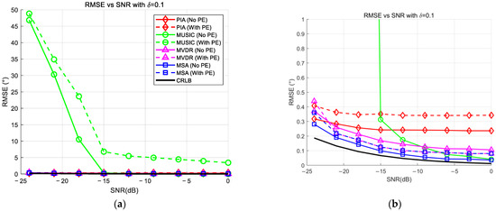
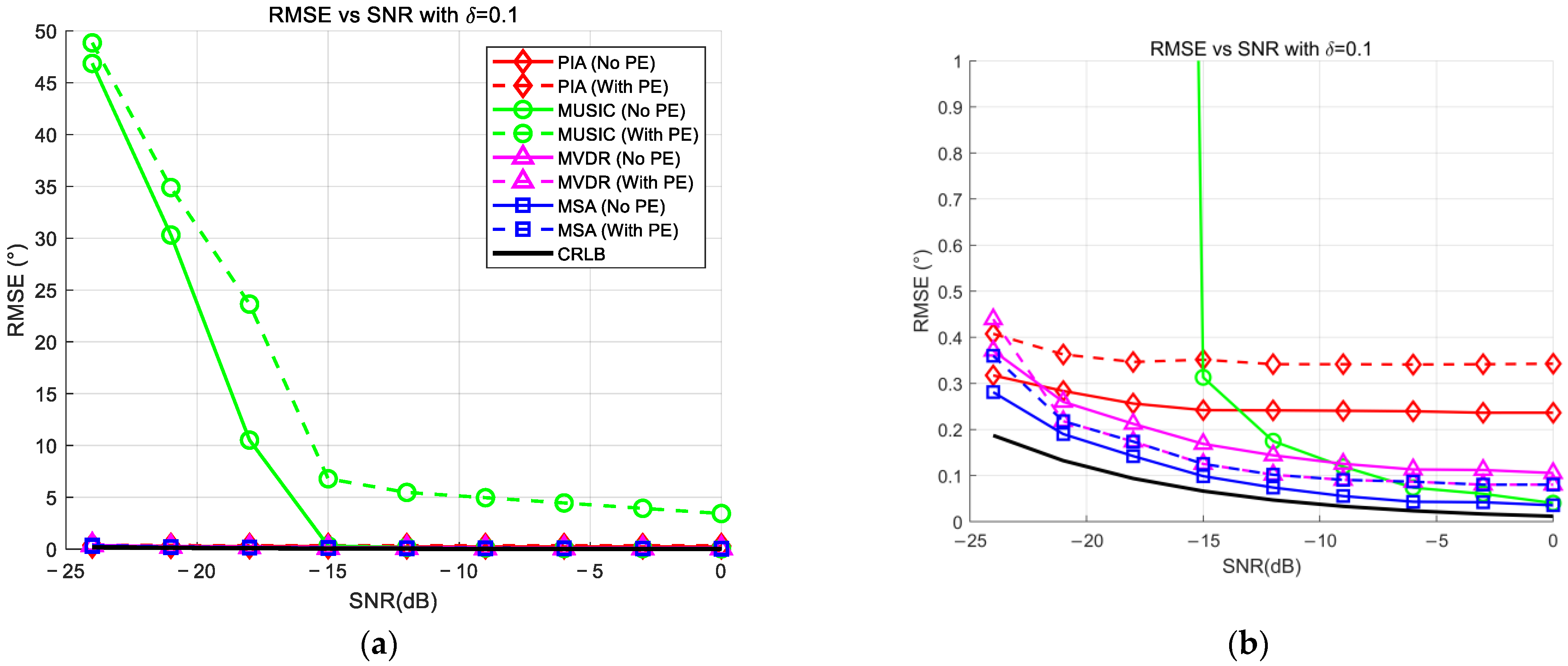
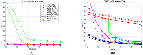
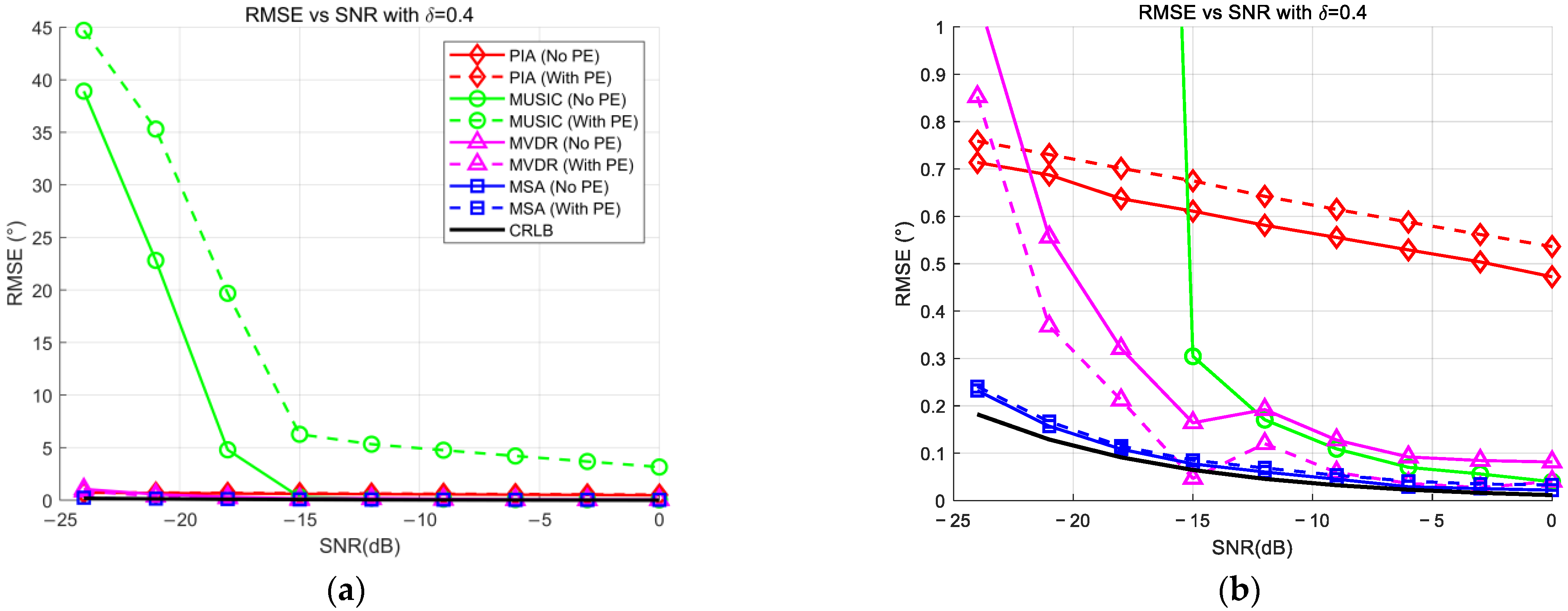
To assess the robustness of the estimators against noise, the RMSE of ${\widehat{\theta }}_T$ as the SNR varies from −24 dB to 0 dB in steps of 3 dB is evaluated. This analysis considers two distinct scenarios for $\delta =0.1$ and $\delta =0.4$, with the peak steering beam index set to $k_p=5$. The results for $\delta =0.1$ are presented in Figure 7, and the results for $\delta =0.4$ are shown in Figure 8, with sub-figures (a) and (b) representing the global view and the locally magnified view, respectively.

Figure 7. RMSE of ${\widehat{\theta }}_T$ versus SNRs with δ = 0.1. (a) original figure (b) zoomed-in view of (a).

Figure 8. RMSE of ${\widehat{\theta }}_T$ versus SNRs with δ = 0.4. (a) Original figure; (b) zoomed-in view of (a).

The global view in Figure 7a illustrates the sensitivity of the estimators to noise. The MUSIC estimator (green lines) exhibits a “waterfall” breakdown, failing to resolve the target when the SNR drops below −21 dB, with errors spiking significantly. In contrast, the proposed MSA estimator (blue lines) and the MVDR estimator (magenta lines) demonstrate superior stability, maintaining valid estimates even at the lowest SNR of −24 dB. The asymptotic performance at higher SNRs is detailed in the magnified view, as shown in Figure 7b. Even with this small deviation, the limitations of the PIA estimator are observable. While the MSA estimator converges to an RMSE of approximately 0.25° in the presence of position errors (dashed blue line), the PIA estimator (red lines) exhibits a higher systematic bias of around 0.45°. This indicates that even for minor grid deviations, the MSA estimator offers improved precision over the parabolic approximation.

The advantages of the proposed method become pronounced when analyzing the large deviation case in Figure 8. Figure 8a reveals that the robustness of the MUSIC estimator deteriorates further as $\delta$ increases. Its breakdown threshold shifts significantly from −21 dB (in Figure 7) to −15 dB. Below this threshold, the MUSIC algorithm suffers from catastrophic failures with RMSEs exceeding 30°. Conversely, the MSA estimator remains exceptionally resilient, exhibiting no breakdown threshold and maintaining consistent accuracy across the entire SNR range down to −24 dB. The magnified view in Figure 8b reveals a fundamental divergence in convergence behaviors. While the MSA estimator and the MVDR show rapid error decay, the PIA estimator exhibits sluggish convergence, limited by a systematic bias lower bound due to model mismatch. Even at 0 dB, the PIA estimator error remains around 0.53°, whereas the MSA estimator achieves a precision of ~0.03°. This order-of-magnitude reduction confirms that the MSA estimator effectively eliminates the systematic bias.

This comparison demonstrates that the MSA estimator offers a superior trade-off. It eliminates the systematic bias that limits the PIA estimator at high SNRs while avoiding the threshold breakdown that plagues MUSIC at low SNRs, making it a highly reliable solution for practical environments.

4.3. Case 3: RMSE of ${\widehat{\theta }}_T$ Versus f₀

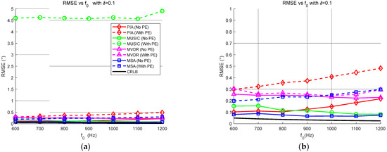
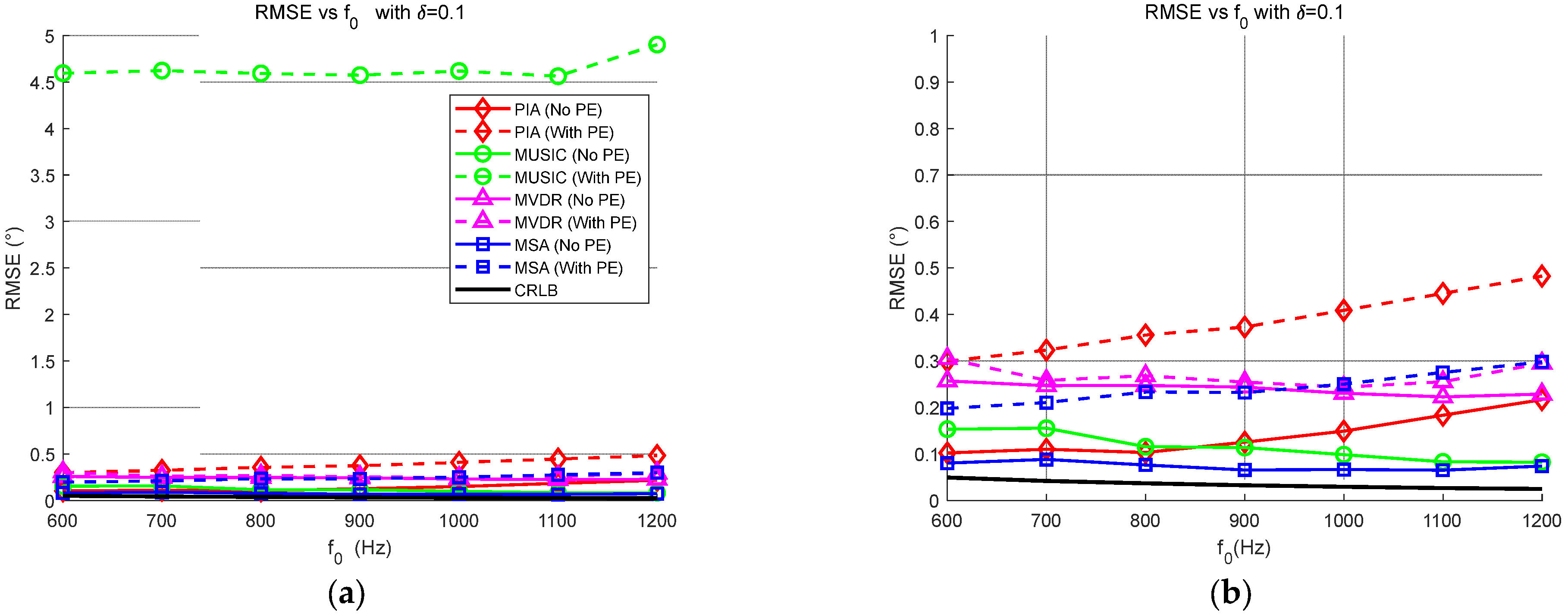
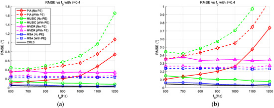
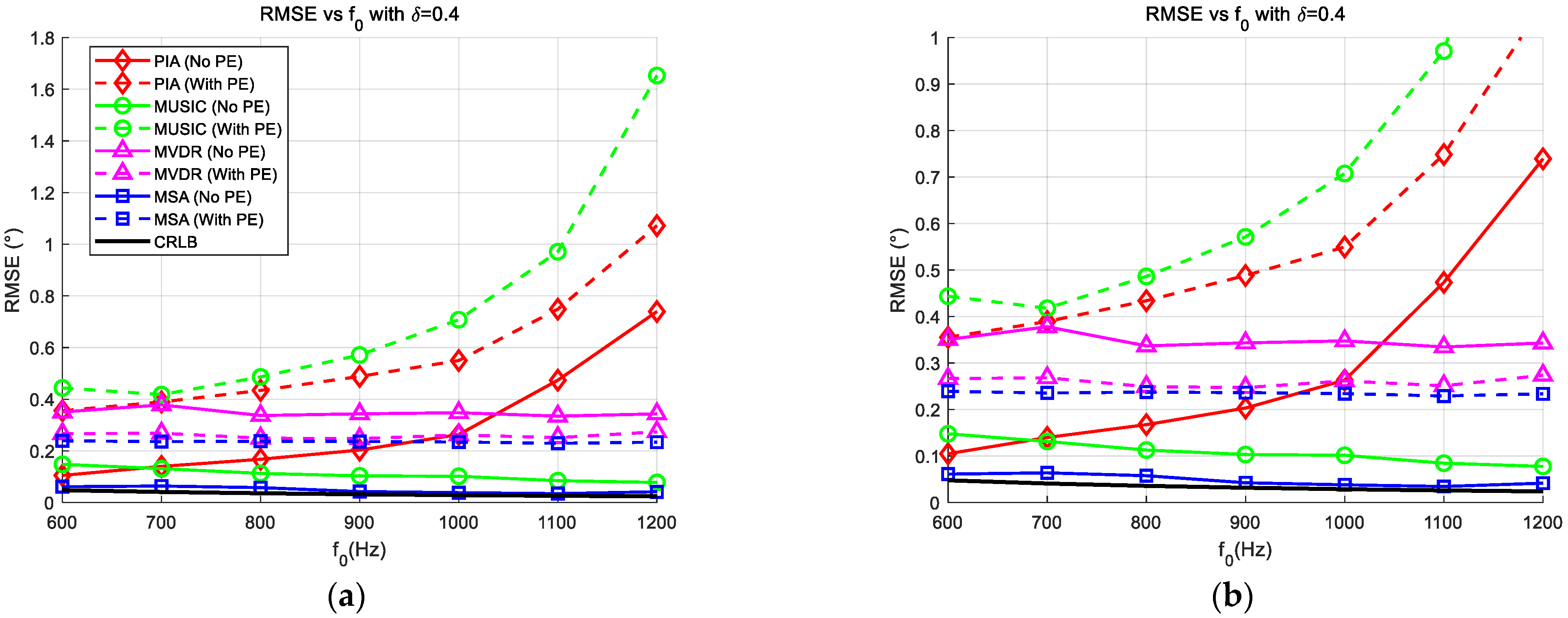
Then, the influence of the signal frequency $f_0$ on the estimation accuracy is investigated. With the SNR fixed at −6 dB, $f_0$ is varied from 600 Hz to 1200 Hz. The peak steering beam index is set to $k_p=5$ (corresponding to 48.19°). Similar to previous sections, two cases are analyzed: $\delta =0.1$ and $\delta =0.4$. The results are presented in Figure 9 and Figure 10, respectively, where subfigure (a) represents the global view and (b) represents the magnified view.

Figure 9. RMSE of ${\widehat{\theta }}_T$ versus f₀ with SNR = −6 dB and δ = 0.1. (a) Original figure; (b) zoomed-in view of (a).

Figure 10. RMSE of ${\widehat{\theta }}_T$ versus f₀ with SNR = −6 dB and δ = 0.4. (a) Original figure; (b) zoomed-in view of (a).

The global view in Figure 9a reveals a significant robustness issue with the MUSIC estimator. In the presence of position errors (green dashed line), MUSIC exhibits severe instability across the entire frequency band, with the RMSE consistently exceeding 4.5°. This indicates that even for small grid deviations, the high-resolution subspace method is extremely sensitive to array manifold perturbations at low SNRs. In contrast, the magnified view in Figure 9b demonstrates the stability of the proposed method. While the PIA estimator (red dashed line) shows a slight upward trend as frequency increases, the proposed MSA estimator (blue dashed line) maintains a low and stable error profile, fluctuating gently around 0.2° ~ 0.3°.

The advantages of the proposed MSA estimator are most pronounced in the large deviation scenario shown in Figure 10. Figure 10a highlights the frequency-dependent degradation of the conventional methods. The MUSIC estimator (green dashed line) shows a clear rising trend, with its RMSE increasing from ~0.4° at 600 Hz to approximately 1.0° at 1200 Hz. Similarly, the PIA estimator exhibits a strong linear dependence on frequency. The magnified view in Figure 10b details this behavior. As the frequency increases from 600 Hz to 1200 Hz, the RMSE of the PIA estimator (solid red line) degrades sharply from ~0.1° to 0.75°. This is physically attributed to the narrowing of the main lobe at higher frequencies, which aggravates the model mismatch between the fixed parabolic template and the actual beam pattern. Conversely, the proposed MSA estimator (blue lines) proves to be effectively frequency-invariant. Regardless of the frequency changes, its RMSE remains remarkably flat at approximately 0.23° (dashed blue line) even with position errors. Quantitatively, at 1200 Hz, the MSA estimator reduces the estimation error by approximately 70% compared to the PIA estimator and avoids the large fluctuations observed in MUSIC. While MVDR exhibits fluctuations between 0.25° and 0.35°, the MSA estimator maintains a lower and smoother error profile. This confirms that the MSA estimator achieves better accuracy than robust adaptive beamformers without incurring the heavy computational cost of matrix inversion.

In summary, the frequency analysis confirms that the proposed MSA estimator effectively decouples the estimation accuracy from signal frequency variations. Unlike the PIA estimator, which suffers from aggravated model mismatch at higher frequencies, and MUSIC, which exhibits significant instability under position errors, the MSA estimator provides a consistent, robust, and high-precision solution across the entire bandwidth.

4.4. Computational Complexity Analysis

To comprehensively evaluate the computational complexity and assess the accuracy and robustness of the proposed method, all simulations were conducted in MATLAB R2022b (The MathWorks, Inc., Natick, MA, USA)on a personal computer running Windows 11, equipped with an AMD Ryzen 7 6800H CPU and 16 GB RAM. To ensure statistical reliability and stable timing measurements, the average execution times and performance metrics were calculated over 1000 independent Monte Carlo trials. The simulation environment and signal parameters remain consistent with the configuration detailed in the previous sections. For the performance assessment, SNR was fixed at −6 dB, and the number of snapshots was set to K = 100.

The computational complexity analysis, summarized in Table 1, reveals significant differences in operational efficiency driven by the specific search grid settings of each algorithm. For the subspace-based methods (MUSIC and MVDR), a fine search grid covering $0^{°}$ to ${180}^{°}$ with a step size of ${0.1}^{°}$ (resulting in L = 1801 search points) was employed to ensure high resolution. Consequently, the MUSIC estimator exhibits the highest computational burden ($\mathcal{O}(M^{2}K+M^3+L{M}^2)$) due to the computationally expensive eigen-decomposition and the exhaustive spectrum search over the fine grid. Similarly, the MVDR estimator requires matrix inversion and fine scanning, resulting in a considerable average execution time of 0.594 ms. In contrast, the interpolation-based estimators (PIA and MSA) utilize a much coarser search grid generated by uniform sampling in the cosine domain, requiring only $N_c=25$ preformed beams. This structural advantage allows both methods to share the efficient coarse beamforming preprocessing step ($\mathcal{O}(M^{2}K+N_c{M}^2)$).

Table 1. Computational complexities and average run time (s).

Methods	Computational Complexity	Average Run Time (s)
MUSIC	$\mathcal{O}(M^{2}K+M^3+L{M}^2)$	$7.64\times {10}^{-4}$
MVDR	$\mathcal{O}(M^{2}K+M^3+L{M}^2)$	$5.94\times {10}^{-4}$
PIA	$\mathcal{O}(M^{2}K+N_c{M}^2)$	$1.45\times {10}^{-4}$
MSA	$\mathcal{O}(M^{2}K+N_c{M}^2+IM)$	$1.99\times {10}^{-4}$

Specifically, the PIA estimator achieves the fastest execution time of 0.145 ms because its refinement stage relies on a closed-form algebraic solution derived from fitting a second-order parabola to three points, which involves negligible computational cost ($\mathcal{O}(1)$). The proposed MSA estimator, while slightly more intensive due to its iterative bisection solver ($I\cdot M,I\approx 16$), maintains a highly comparable execution time of 0.199 ms. As validated by the simulation results, the MSA estimator is approximately 3.8 times faster than MUSIC and 2.9 times faster than MVDR. This confirms that the slight computational increase in the MSA estimator over the PIA estimator is minimal and well-justified by the significant accuracy improvements and bias elimination demonstrated in the previous sections, making the MSA estimator a highly efficient solution for real-time high-precision applications.

4.5. DOA Estimation Performance Under NULA

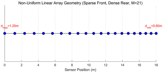
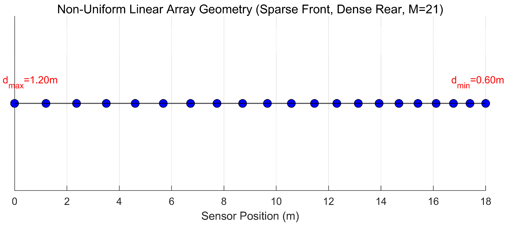
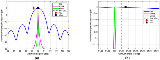
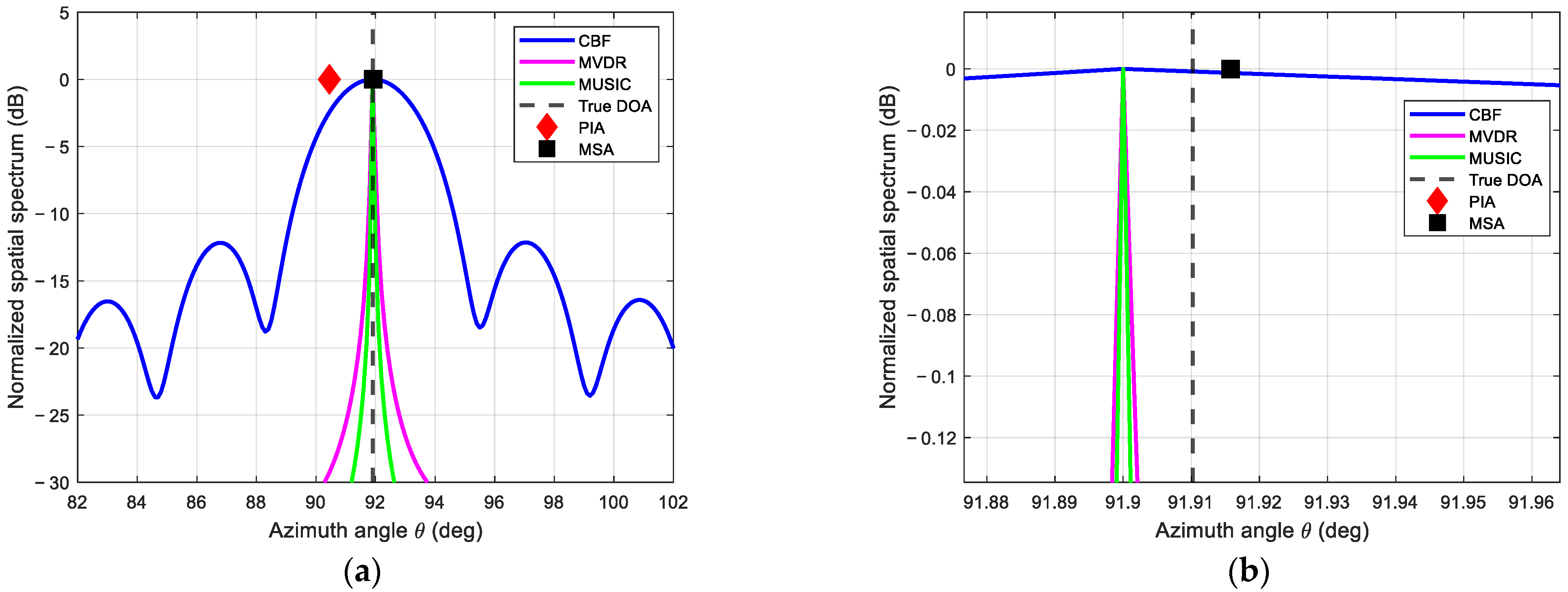
To verify the generalization capability and estimation precision of the proposed estimator under arbitrary geometries, simulations are conducted using a NULA configuration, as illustrated in Figure 11. The array comprises $M=21$ sensors with inter-element spacing linearly decreasing from $d_{\max }=1.20$ m to $d_{\min }=0.60$ m. The simulation was set up with a single target located at the precise angle of ${\theta }_T={91.9102}^{°}$ (corresponding to $\delta =0.4$) under an SNR of −6 dB. The estimated spatial spectra are presented in Figure 12. From the global spectrum view in Figure 12a, the CBF estimator shows high sidelobes due to the irregular geometry, while MUSIC and MVDR form sharp peaks near the true DOA. However, the locally magnified view in Figure 12b reveals quantitative performance disparities. Specifically, the PIA estimator (red diamond) fails to locate the target accurately, yielding an estimated DOA of ${90.4362}^{°}$. This results in a substantial bias of approximately ${1.4740}^{°}$, as the asymmetric main lobe of the NULA violates the parabolic assumption required for polynomial fitting. In stark contrast, the proposed MSA estimator (black square) achieves an estimation of ${91.9081}^{°}$, resulting in a negligible error of only ${0.0021}^{°}$. This quantitative comparison demonstrates that the proposed MSA estimator effectively corrects the geometric mismatch errors, matching the high precision of subspace-based methods like MUSIC (which also converge near ${91.9}^{°}$) while significantly outperforming conventional interpolation techniques in non-uniform array scenarios.

Figure 11. View of the NULA configuration.

Figure 12. DOA estimation results under NULA configuration. (a) Original figure; (b) zoomed-in view of (a).

Extensive simulations validate the robustness of the proposed MSA estimator. Specifically, it maintains a stable RMSE of ~0.12°, eliminating the catastrophic > 3.8° error spikes seen in MUSIC, and extends the operational range to −24 dB, surpassing MUSIC’s −15 dB breakdown threshold. Furthermore, the MSA estimator achieves frequency-invariant precision of ~0.23°, significantly outperforming the PIA estimator, which degrades to 0.75° due to model mismatch. Finally, the proposed method retains low computational complexity and generalizes effectively to arbitrary array geometries without accuracy loss.

5. Conclusions

Robust DOA estimation is a critical task in underwater acoustic engineering, yet the performance of traditional high-resolution subspace methods often degrades severely when facing sensor position errors and limited snapshots. In this paper, a novel Model Solution Algorithm (MSA) estimator is proposed to address the precision limitations of the Conventional Beamformer by numerically solving the exact beam pattern equation. Quantitative simulations demonstrate that the MSA estimator offers a superior trade-off between accuracy, robustness, and efficiency. Specifically, the estimator maintains a stable RMSE of approximately 0.12° even under sensor position errors, effectively eliminating the catastrophic error spikes exceeding 3.8° observed in the MUSIC estimator. Furthermore, the proposed method exhibits exceptional noise resilience by extending the operational range down to −24 dB, significantly surpassing the −15 dB breakdown threshold of MUSIC. In terms of frequency invariance, the MSA estimator achieves a consistent precision of ~0.23° across the bandwidth, outperforming the PIA estimator, which degrades to 0.75° due to severe model mismatch. Additionally, the results confirm that the proposed method preserves a low computational complexity suitable for real-time applications and can be effectively generalized to arbitrary array geometries, such as non-uniform linear arrays, without accuracy loss.

Despite these advantages, the current derivation is primarily optimized for single-source estimation in narrowband scenarios, which constitutes a limitation in complex interference environments. Future work will focus on extending the MSA estimator to multi-target estimation, potentially through iterative beam-space cancelation techniques to handle overlapping main lobes. Additionally, future work will aim to generalize the method to wideband frequency-modulated signals by integrating it with time-frequency analysis tools such as the Short-Time Fourier Transform (STFT) and to adapt it for two-dimensional planar array geometries.

References

- Yu, G. Eigenbeam-space transformation based steerable differential beamforming for linear arrays. Signal Process. 2023, 212, 109171. [Google Scholar] [CrossRef] [Scilit]
- Bellili, F.; Souheib, B.A.; Affes, S.; Ghrayeb, A. Low-complexity DOA estimation from short data snapshots for ULA systems using the annihilating filter technique. EURASIP J. Adv. Signal Process. 2017, 2017, 48. [Google Scholar] [CrossRef] [Scilit]
- Blostein, S.D.; Leib, H. Multiple antenna systems: Their role and impact in future wireless access. IEEE Commun. Mag. 2003, 41, 94–101. [Google Scholar] [CrossRef]
- Zhou, C.; Gu, Y.; Fan, X.; Shi, Z.; Mao, G.; Zhang, Y.D. Direction-of-Arrival Estimation for Coprime Array via Virtual Array Interpolation. IEEE Trans. Signal Process. 2018, 66, 5956–5971. [Google Scholar] [CrossRef] [Scilit]
- Huang, Y.; Zhou, M.; Vorobyov, S.A. New Designs on MVDR Robust Adaptive Beamforming Based on Optimal Steering Vector Estimation. IEEE Trans. Signal Process. 2019, 67, 3624–3638. [Google Scholar] [CrossRef] [Scilit]
- Yan, F.; Jin, M.; Liu, S.; Qiao, X. Real-Valued MUSIC for Efficient Direction Estimation With Arbitrary Array Geometries. IEEE Trans. Signal Process. 2014, 62, 1548–1560. [Google Scholar] [CrossRef] [Scilit]
- Yan, F.G.; Jin, M.; Zhou, H.J.; Wang, J.; Liu, S. Low-degree root-MUSIC algorithm for fast DOA estimation based on variable substitution technique. Sci. China Inf. Sci. 2020, 63, 152201. [Google Scholar] [CrossRef] [Scilit]
- Yan, F.G.; Shen, Y.; Jin, M. Fast DOA estimation based on a split subspace decomposition on the array covariance matrix. Signal Process. 2015, 115, 1–8. [Google Scholar] [CrossRef] [Scilit]
- Li, H.; Ichige, K.; Arai, H. A closed-form DOA estimation formula of multiple coherent waves for uniform linear array. In Proceedings of the 2011 4th International Congress on Image and Signal Processing, Shanghai, China, 15–17 October 2011; pp. 2588–2592. [Google Scholar]
- Li, B.; Bai, W.; Zheng, G. Successive ESPRIT algorithm for joint DOA-range-polarization estimation with polarization sensitive FDA-MIMO radar. IEEE Access 2018, 6, 36376–36382. [Google Scholar] [CrossRef] [Scilit]
- Liu, F.L.; Wang, X.P.; Huang, M.X.; Wan, L.; Wang, H.; Zhang, B. A Novel Unitary ESPRIT Algorithm for Monostatic FDA-MIMO Radar. Sensors 2020, 20, 827. [Google Scholar] [CrossRef] [Scilit] [PubMed]
- Wang, Y.; Zhao, L.; Qiu, L.; Wang, J.; Li, C. A Sparse Bayesian Learning Method for Direction of Arrival Estimation in Underwater Maneuvering Platform Noise. J. Mar. Sci. Eng. 2023, 11, 1879. [Google Scholar] [CrossRef] [Scilit]
- Yang, Z.; Zhang, X.; Luo, Z.; Shen, T.; Cui, M.; Li, X. Parallel net: Frequency-decoupled neural network for DOA estimation in underwater acoustic detection. J. Mar. Sci. Eng. 2025, 13, 724. [Google Scholar] [CrossRef] [Scilit]
- Zhou, L.; Zhou, S.; Qi, Y.; Wu, L.; Benezeth, Y. A deep shrinkage network for direction-of-arrival estimation with sparse prior. J. Mar. Sci. Eng. 2025, 13, 206. [Google Scholar] [CrossRef] [Scilit]
- Yang, T.C. Deconvolved Conventional Beamforming for a Horizontal Line Array. IEEE J. Ocean. Eng. 2018, 43, 160–172. [Google Scholar] [CrossRef] [Scilit]
- Mini, P.R.; Mridula, S.; Mohanan, P. An approach for side lobe reduction in conventional beamformers. In Proceedings of the 2012 Annual IEEE India Conference (INDICON), Kochi, India, 7–9 December 2012; pp. 794–797. [Google Scholar]
- Hacker, P.; Yang, B. Single snapshot DOA estimation. Adv. Radio Sci. 2010, 8, 251–256. [Google Scholar] [CrossRef] [Scilit]
- Raich, R.; Goldberg, J.; Messer, H. Bearing estimation for a distributed source via the conventional beamformer. In Proceedings of the Ninth IEEE Signal Processing Workshop on Statistical Signal and Array Processing, Portland, OR, USA, 14–16 September 1998; pp. 5–8. [Google Scholar]
- Li, Q.; Yi, L. The problem of precise bearing and automatic tracking for target in digital sonar. Acta Acust. 1996, 21, 709–713. [Google Scholar]
- Stoica, P.; Nehorai, A. Performance study of conditional and unconditional direction-of-arrival estimation. IEEE Trans. Acoust. Speech Signal Process. 1990, 38, 1783–1795. [Google Scholar] [CrossRef] [Scilit]
- Kay, S.M. Fundamentals of Statistical Signal Processing, Volume I: Estimation Theory; Prentice-Hall: Upper Saddle River, NJ, USA, 1993. [Google Scholar]
- Gray, D. Effect of time-delay errors on the beam pattern of a linear array. IEEE J. Ocean. Eng. 1985, 10, 269–277. [Google Scholar] [CrossRef] [Scilit]
- Knight, W.C.; Pridham, R.G.; Kay, S.M. Digital signal processing for sonar. Proc. IEEE 1981, 69, 1451–1506. [Google Scholar] [CrossRef] [Scilit]
Disclaimer/Publisher’s Note: The statements, opinions and data contained in all publications are solely those of the individual author(s) and contributor(s) and not of MDPI and/or the editor(s). MDPI and/or the editor(s) disclaim responsibility for any injury to people or property resulting from any ideas, methods, instructions or products referred to in the content. |
© 2026 by the authors. Licensee MDPI, Basel, Switzerland. This article is an open access article distributed under the terms and conditions of the Creative Commons Attribution (CC BY) license.