Construction of Typical Sailing Conditions for Harbor Tugs Based on WOA-K-Means++ Clustering and Hidden Markov Models

Abstract

The global shipping industry faces severe carbon emission challenges. Harbor tugs, as significant contributors to port emissions, require improved energy efficiency. However, their sailing conditions are complex and dynamic, making temporal feature characterization difficult with traditional static or simplistic clustering methods. To address this, this study proposes a novel method for constructing typical sailing conditions by integrating an enhanced clustering approach with Hidden Markov Models (HMM). First, kinematic segments are extracted from processed ship speed data, and key features are selected and reduced via Principal Component Analysis (PCA). Subsequently, an improved clustering model combining the Whale Optimization Algorithm (WOA) and K-means++ is developed to categorize segments into six distinct condition types. These clustered states then serve as the hidden states of an HMM, whose learned transition matrix synthesizes a 3600 s typical sailing condition profile. The constructed profile is validated through multi-dimensional comparison with original data, demonstrating high fidelity in statistical characteristics, temporal properties, and distribution similarity. The results confirm that the proposed method can accurately replicate the operational patterns of harbor tugs. This study provides a reliable data foundation for the energy efficiency assessment and optimization of harbor tugs and offers a new methodological perspective for constructing operational profiles for ships and other mobile machinery.

1. Introduction

1.1. Background

With the increasingly pressing issue of global climate change, reducing greenhouse gas emissions has become a common goal for the international community [1]. The shipping industry accounts for approximately 3% of total global anthropogenic emissions, with a persistent upward trend. Ports, as critical nodes within the global shipping and logistics chain, face particularly urgent demands for green and low-carbon transformation [2]. As a special and important category of mobile emission sources, harbor tugs play an irreplaceable role in assisting large ships with berthing, unberthing, and towing operations [3]. These ships exhibit extremely complex dynamic operational characteristics during service, including frequent start-stop cycles, intense load fluctuations, extended periods of low-load standby, and short bursts of high-power output [4]. Such patterns often force main engines to operate outside their optimal fuel efficiency ranges, leading to persistently high energy consumption and emissions. Current pathways for improving the energy efficiency of these ships mainly include hull optimization, propulsion system upgrades, and operational strategy improvements [5]. Regardless of the specific technical approach adopted, an accurate description and quantitative analysis of their actual operating conditions are fundamental prerequisites. Constructing a typical sailing condition that authentically reflects speed variations, power demand, acceleration characteristics, and the temporal correlation of operational patterns is crucial. Such a profile serves as an essential foundation for evaluating energy efficiency, designing new systems, formulating optimization strategies, and accurately predicting energy consumption and emissions. It is also key to advancing port emission reduction efforts and optimizing powertrain design and energy management. Therefore, research focused on developing a typical sailing condition for harbor tugs is of significant importance for promoting green port development and achieving regional sustainability.

1.2. Limitations of Existing Approaches

The methodology for constructing typical driving cycles is well-established in the automotive field, as exemplified by standardized test cycles like the New European Driving Cycle (NEDC) and the Worldwide Harmonized Light Vehicles Test Procedure (WLTP), which are widely used for fuel consumption and emission certification [6]. Such standard cycles are typically developed based on extensive real-world road data, employing statistical analysis combined with predefined parameters [7]. In contrast, research on operational profile construction for ships started later. Existing assessment metrics, such as the Energy Efficiency Design Index (EEDI) for new ships and the Energy Efficiency Existing Ship Index (EEXI), largely rely on static design parameters and struggle to accurately reflect the dynamic performance of ships under actual operating conditions [8]. This is particularly problematic for harbor tugs, which operate under extremely complex conditions; directly applying these static indices can lead to significant errors. The maritime industry has not yet developed a unified, standardized sailing condition analogous to those in the automotive sector. The primary reasons include the strong influence of multiple dynamic factors on ship operation, such as waterway environment, meteorological conditions, the ship’s own state, and mission requirements, which result in a wide range of load variations. Furthermore, substantial differences exist among ship types, propulsion systems, and routes, making the development of a universal standard both highly difficult and costly [9].

1.3. Adaptation of Vehicle Driving Cycles

As a specialized ship type dedicated to port tasks like berthing/unberthing and towing, the operational profile of a harbor tug is characterized by distinct patterns of “low speed with high torque, rapid speed changes, and slow stopping” [10]. This dynamic operational mode bears a high degree of similarity to the driving characteristics of urban buses, construction vehicles, and other machinery operating under stop-and-go or congested conditions. There is an essential isomorphism between them in terms of the morphology of speed-time sequences and the distribution of key statistical parameters. Consequently, the mature methodologies for constructing vehicle driving cycles can be effectively adapted and applied to harbor tugs. Specifically: at the data acquisition level, high-frequency time-series data collection can be achieved using onboard data loggers [11]; during the feature analysis stage, feature parameters commonly used in vehicle studies can be adopted to quantify operational intensity, and clustering methods can be utilized to identify representative kinematic segments [12]; in the profile construction phase, well-established methods from the automotive domain, such as the “short-segment concatenation method” or “Markov chain” approaches, can be employed. These methods combine typical kinematic segments according to their transition probabilities in actual operation, thereby constructing a typical sailing condition that not only comprehensively reflects a specific operational cycle but also possesses statistical representativeness and engineering practicality [13,14]. This research approach, grounded in the similarity of operational characteristics rather than the type of vehicle, not only provides a critical benchmark for optimizing the energy efficiency of harbor tugs, enabling precise emission assessment, and facilitating the development of new energy propulsion systems, but also opens up a technical pathway with both theoretical innovation and significant engineering application value.

1.4. Research Gap and Contributions

In summary, despite significant progress in vehicle driving cycle construction and its inspiration for harbor tug research, core challenges remain: (1) Traditional clustering algorithms (e.g., K-means, K-means++) are sensitive to initial centers and prone to local optima when handling the high-dimensional, non-stationary operational data of tugs, compromising the accuracy of state partitioning; (2) While some studies combine metaheuristics with clustering, or clustering with sequence models, a complete and robust framework specifically tailored for tug operational characteristics—spanning from globally optimized clustering to temporal dynamics synthesis—is still lacking. To address the aforementioned challenges, this study proposes an integrated innovation framework. Its core methodological contributions are: Firstly, it innovatively integrates the Whale Optimization Algorithm (WOA) with K-means++ to form a hybrid WOA-K-means++ clustering model. This model leverages the strong global search capability of WOA to provide near-optimal initial cluster centers for K-means++, effectively overcoming the initialization sensitivity and local optimum problems of traditional methods when partitioning complex tug kinematic segments, leading to more accurate and stable identification of sailing states. Secondly, it systematically defines the optimized cluster states as the hidden states of a Hidden Markov Model (HMM). The HMM learns the transition probabilities between states from real sailing data and synthesizes the typical sailing condition sequence based on this. This series framework of ‘optimized clustering + HMM sequence modeling’ not only ensures the representativeness of the synthesized profile in terms of feature statistics but, more crucially, preserves the temporal logic and dynamic characteristics of state evolution in the original data. Consequently, it generates a typical sailing condition for harbor tugs that possesses both high fidelity and engineering practicality.

In recent years, with advancements in intelligent and sensor technologies, data-driven methods for constructing operational profiles based on large-scale measured data have emerged as a significant research focus [15]. Currently, the technical approaches in this field can be broadly categorized into two main types. The first type is the statistical feature-based construction method. This approach involves performing statistical analysis on extensive historical operational data to extract the probability distribution characteristics of key parameters such as speed, acceleration, and power. A synthetic profile sequence that conforms to these statistical properties is then generated [16]. For example, Ref. [17] proposed a composite stochastic model for real-time freeway traffic simulation. This model considers the joint distribution of speed and acceleration and utilizes Monte Carlo simulation to generate random traffic profiles, effectively capturing the spatiotemporal characteristics and uncertainties of traffic flow. The advantage of such methods lies in their ability to faithfully reproduce the macroscopic statistical patterns of the data. However, they often overlook the temporal correlations between successive operational states and the intrinsic logic governing mode transitions, which can result in generated profiles lacking realism in their temporal structure [18]. The second type is the hybrid method based on clustering and sequence modeling. This method first employs clustering algorithms to segment continuous operational data into several discrete operational modes (or segments) with clear physical meanings. Subsequently, sequence modeling techniques, such as Markov chains, are used to describe the transition rules between these modes [19]. Regarding clustering algorithms, the K-means algorithm is widely adopted due to its simplicity and efficiency. However, the traditional K-means algorithm is sensitive to the initial cluster centers, prone to converging to local optima, and its performance is limited when handling high-dimensional, non-convex datasets [20]. To address these limitations, researchers have proposed improved algorithms such as K-means++ [21], Fuzzy C-Means (FCM) [22], and Density-Based Spatial Clustering of Applications with Noise (DBSCAN) [23]. For instance, ref. [24], aiming to overcome K-means’ sensitivity to outliers and the difficulty in determining the optimal K value, proposed a method for constructing electric vehicle driving cycles based on hierarchical clustering. This method first applies wavelet denoising to real driving data, segments the data, extracts microscopic trip feature parameters, performs classification via hierarchical clustering, and finally selects representative segments based on their proportions to synthesize the driving cycle. Subsequent simulation and statistical analysis verified the accuracy of the constructed profile. Ref. [25] proposed a K-means clustering method based on an improved Particle Swarm Optimization (PSO) algorithm, enhancing its global search capability. This method was applied to actual driving data from Jinan City, successfully constructing a local typical driving cycle through Principal Component Analysis (PCA) and clustering. In terms of sequence modeling, Markov chains are a common tool for describing state transition probabilities [26]. However, first-order Markov chains only consider the direct influence of the current state on the next state, making it difficult to capture long-term dependencies [27]. The HMM, as a type of probabilistic graphical model, introduces the concept of hidden states. This allows it to better characterize the latent dynamic mechanisms behind observed sequences, making it particularly suitable for modeling complex time-series data with underlying operational modes [28]. For example, ref. [29] proposed a method for constructing urban tour bus driving cycles by combining GA-K-means (GA, Genetic Algorithm) with HMM. By using the HMM to capture the state transition characteristics of the speed sequence, the method achieved more accurate driving mode recognition and profile generation.

To provide a more systematic overview of existing methods for constructing typical operational profiles and to clarify the positioning of this study,

Table 1. Comparative Analysis of Related Studies on Typical Operational Profile Construction Methods.

Reference	Objective	Methodology	Dataset	Decision Variables/Features	Solution Approach	Limitations	Gap Analysis
[17] Brady et al.	Generate random traffic/driving profiles based on statistical distributions.	Monte Carlo simulation, joint speed-acceleration distribution.	Highway vehicle data.	Speed, acceleration.	Random sequence generation.	Ignores temporal correlations between states, lacks realistic dynamic logic.	Focuses on macro-statistical reproduction, does not cluster micro-trips or model sequences based on state transitions.
[24] Jing et al.	Construct typical driving cycle for electric vehicles.	Wavelet denoising, hierarchical clustering, segment selection and splicing.	Real-world EV data.	Microscopic trip feature parameters.	Hierarchical clustering and representative segment selection.	Clustering algorithm (hierarchical) may be less efficient; final cycle splicing does not consider transition probabilities between segments.	Uses clustering but does not optimize initial center selection; profile synthesis is simple statistical selection, not using temporal models (e.g., Markov chain) to simulate state transitions.
[25] Yan et al.	Construct local typical driving cycle.	Improved PSO-optimized K-means, Principal Component Analysis.	Real driving data from Jinan City.	Multi-dimensional driving features.	PSO-K-means clustering, PCA for dimensionality reduction.	PSO algorithm may suffer from premature convergence; does not explicitly use clustering results for temporal sequence generation.	Employs a metaheuristic to optimize clustering but does not integrate the optimized clusters with a model capable of capturing temporal dynamics (e.g., HMM) for profile synthesis.
[29] Yuan et al.	Construct driving cycle for urban tour buses.	GA-K-means clustering combined with HMM.	Beijing tour bus data.	Kinematic segment features.	GA-optimized clustering, HMM for sequence modeling and generation.	GA has complex parameter tuning and potentially slower convergence; no specific optimization for clustering initialization in high-dimensional, non-convex feature spaces.	Proposes a clustering + HMM framework, but the metaheuristic used for optimizing cluster centers (GA) may not be the optimal choice in terms of global search capability and convergence speed.
This work	Construct typical sailing condition for harbor tugs.	WOA-K-means++ clustering combined with HMM.	AIS (Automatic Identification System) and voyage data of tugs from Port of Dalian.	13-dimensional kinematic and time proportion features.	PCA for dimensionality reduction, WOA for global optimization of cluster centers, HMM for learning state transitions and synthesizing sequences.	Data from a single port and ship type; parameters and proportions require calibration for new environments.	1. Introduces WOA to optimize initial centers for K-means++, enhancing clustering stability and accuracy for high-dimensional non-convex data. 2. Explicitly uses the optimized cluster states as hidden states of an HMM, utilizing its transition matrix to synthesize a typical profile with both statistical representativeness and temporal rationality.

summarizes the key elements and limitations of representative research in related fields.

In light of the limitations of existing methods for constructing vehicle driving cycles and the research gap in developing typical sailing conditions for harbor tugs, there is a pressing need to develop a data-driven methodology that offers both high robustness and strong interpretability. This method must be capable of accurately partitioning the highly non-stationary operational data of harbor tugs into distinct states and, based on this partitioning, generating a high-fidelity typical sailing condition profile. While metaheuristic optimizers such as PSO and GA have been applied to clustering initialization, they may suffer from premature convergence or high parameter sensitivity. In contrast, the WOA, inspired by the bubble-net hunting behavior of humpback whales, exhibits stronger global search capability, faster convergence, and fewer control parameters, making it particularly suitable for optimizing the initial centers of K-means++ in high-dimensional, non-convex datasets [30,31]. To address this, the present study proposes an innovative integrated framework that establishes a comprehensive technical workflow encompassing “data processing, feature dimensionality reduction, clustering optimization, temporal sequence synthesis, and comprehensive validation.” The core concept is outlined as follows: First, the original ship speed data undergoes processing and feature extraction. Subsequently, PCA is employed to reduce the dimensionality of the high-dimensional feature set, thereby enhancing the efficiency and stability of subsequent processing steps. Then, to address the shortcomings of traditional clustering algorithms, the WOA is introduced to perform a global search for the optimal initial cluster centers for the K-means++ algorithm. This integration results in a WOA-K-means++ clustering model, aimed at achieving a more precise and stable partitioning of kinematic segments. Next, the optimal clustering results are used to define the hidden states of an HMM. The state transition probability matrix derived from this HMM is subsequently utilized to synthesize the typical sailing condition profile. Finally, a multi-level validation framework, integrating statistical properties, time-domain correlations, and frequency-domain characteristics, is established to quantitatively assess the validity of the constructed typical sailing condition.

In summary, a key gap persists in constructing a typical operational profile for harbor tugs: the lack of a robust and integrated framework that simultaneously ensures the accuracy of micro-kinematic state partitioning (overcoming the limitations of traditional clustering algorithms) and the authenticity of macro-temporal evolution logic (surpassing simple statistical splicing). This study aims to bridge this specific gap. The main contributions of this study can be summarized as follows:

(1)

An integrated clustering method combining the WOA and K-means++ (WOA-K-means++) is proposed, which achieves global optimization of cluster center selection and enhances the accuracy and stability of kinematic segment classification.

(2)

A condition synthesis method based on an HMM is proposed, which effectively captures the temporal correlations and state transition characteristics among real kinematic segments.

(3)

A 3600 s typical sailing condition profile for harbor tugs is constructed, and the rationality and validity of the constructed condition are verified through comparative analysis using multiple evaluation metrics.

2. Materials and Methods

2.1. Research Subject

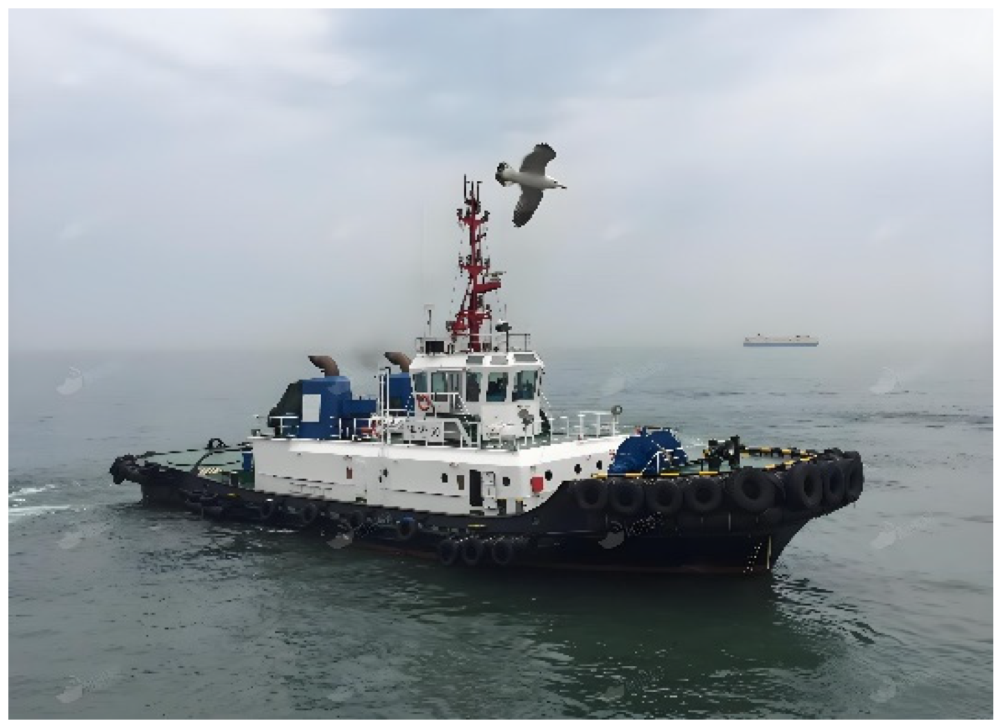
Figure 1 presents the prototype ship for this study—a typical harbor tug operating in the Port of Dalian. As a primary workhorse ship in this port area, its main function is to assist large container ships, bulk carriers, and tankers during berthing and unberthing operations. To comply with emission control requirements within the port zone, this tug employs a series hybrid power system with a range extender. Its key technical specifications are listed in

Table 2. Key Technical Specifications of the Typical Harbor Tug at the Port of Dalian.

Indicator	Parameter
Length Overall (LOA)	35 m
Beam	12 m
Draft	5.3 m
Builder	Jiangsu Zhenjiang Shipyard (Group) Co., Ltd., Zhenjiang, China
Ship Type	Azimuth Stern Drive (ASD) Tug
Owner	Dalian Port (Group) Co., Ltd., Dalian, China
Main Engine Power	7200 horsepower
Typical Sailing Condition Definitions
Low-Speed Harbor Berthing/Unberthing	Ship speed: 0–2 knots
Slow-Speed Harbor/Coastal Transit	Ship speed: 2–4 knots
Conventional Medium-Low Speed Cruising	Ship speed: 4–8 knots
Medium-Speed Towing	Ship speed: 8–10 knots
High-Speed Sailing	Ship speed: 10–13 knots
Full-Speed/Emergency Sailing	Ship speed: 13–15 knots

. This harbor tug features high power, high bollard pull, and excellent maneuverability, utilizing advanced 360-degree azimuth propulsion technology. This allows it to provide thrust in any direction, resulting in superior handling and flexibility to meet diverse operational demands such as assisting large ships, harbor towing, and emergency response. Its compact hull design, combined with a powerful propulsion system, determines that its sailing profile is characterized by typical dynamic features of “short cycles, frequent speed changes, and sudden load shifts.” This serves as the physical basis for the detailed segmentation and clustering of the ship’s speed-time data in this study. Based on actual operational requirements, the sailing conditions of the harbor tug can be categorized into six types (see Table 2), each with defined speed ranges and operational characteristics:

(1)

Low-Speed Harbor Berthing/Unberthing Condition (0–2 knots): Requires the highest level of maneuvering precision, involving the provision of stable thrust at extremely low speeds to assist large ships in making smooth contact with or departing from the berth.

(2)

Slow-Speed Harbor/Coastal Transit Condition (2–4 knots): Suitable for repositioning within complex waterways, balancing maneuverability with moderate thrust.

(3)

Conventional Medium-Low Speed Cruising Condition (4–8 knots): Primarily used for longer-distance transfers within the harbor or along the coast, typically representing the upper limit of safe harbor speed, balancing efficiency and safety.

(4)

Medium-Speed Towing Condition (8–10 knots): Applicable for towing tasks with specific speed requirements, providing a cost-effective bollard pull within this range.

(5)

High-Speed Sailing Condition (10–13 knots): Used for rapid repositioning or emergency response, approaching the ship’s conventional maximum speed.

(6)

Full-Speed/Emergency Sailing Condition (13–15 knots): Activated only in extreme situations such as salvage operations, during which load and fuel consumption increase significantly.

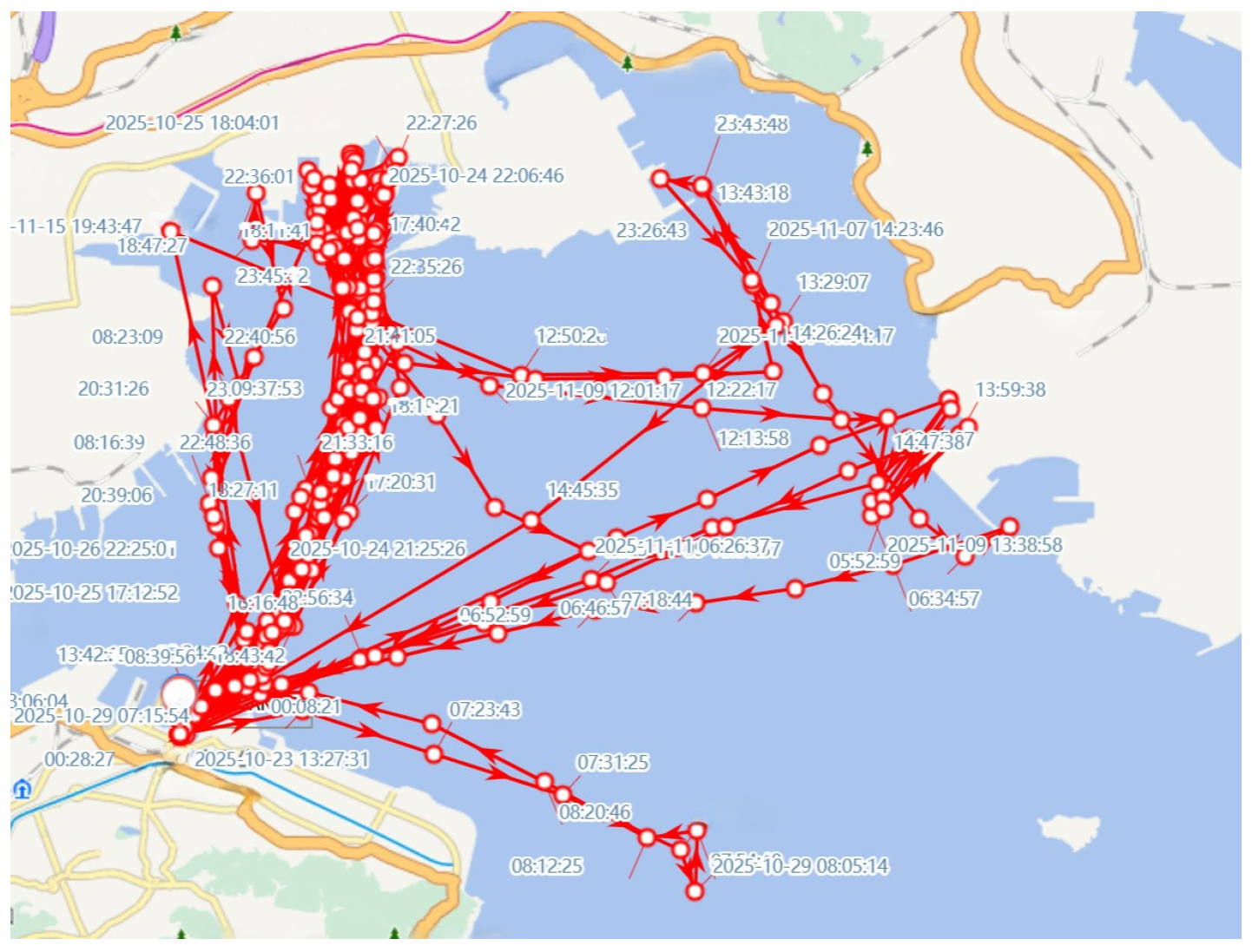
It is important to note that the effective bollard pull of a harbor tug decreases sharply as speed increases. When the speed exceeds 5–7 knots, most of the thrust is consumed in overcoming the tug’s own resistance, significantly diminishing its assisting effect on large ships. This speed point is therefore considered the operational “limiting speed.” This physical characteristic fundamentally explains why medium- and low-speed conditions dominate actual harbor operations. Figure 2 clearly presents the typical sailing trajectory of this harbor tug over a period, overlaid on a map of the port waters, which corresponds to and generated the original ship speed data required for this study. The trajectory exhibits distinct spatial characteristics of high density, numerous turning points, and a winding path, markedly different from the straight-line courses of ocean-going ships. This visually reflects the spatial constraints and task complexity faced by harbor tugs operating within confined waters such as docks, channels, and anchorages. Low-speed lingering segments in the trajectory correspond to operations requiring fine control, such as pushing and escorting. Short-distance high-speed movement segments represent transit between different operational points. Dense circling trajectories near berths are directly related to assisting large ships with berthing and unberthing. This figure provides a geographical and operational rationale at the macro spatial movement level for the various condition modes—such as low speed, medium speed, high speed, and frequent start-stops—evident in the ship speed data. Consequently, it reveals the real operational scenarios and spatial constraints underlying the ship’s speed-time series. It should be noted that the dataset used in this study originates from a single port (Dalian) and a specific type of azimuthing tug. Although this may limit the direct generalization of exact numerical thresholds or operating condition ratios to other ports or tug types, the proposed methodological framework, consisting of data preprocessing, feature engineering, WOA-K-means++ clustering, and HMM-based synthesis, is designed to be versatile and data-adaptive. The core algorithm operates on feature vectors and state sequences that can be extracted from any similar time-series operational data. Therefore, as long as representative local data is collected for calibration and validation, the method is conceptually transferable to other port tugs, and even to other types of engineering ships operating in constrained and dynamic environments.

2.2. Research Methods

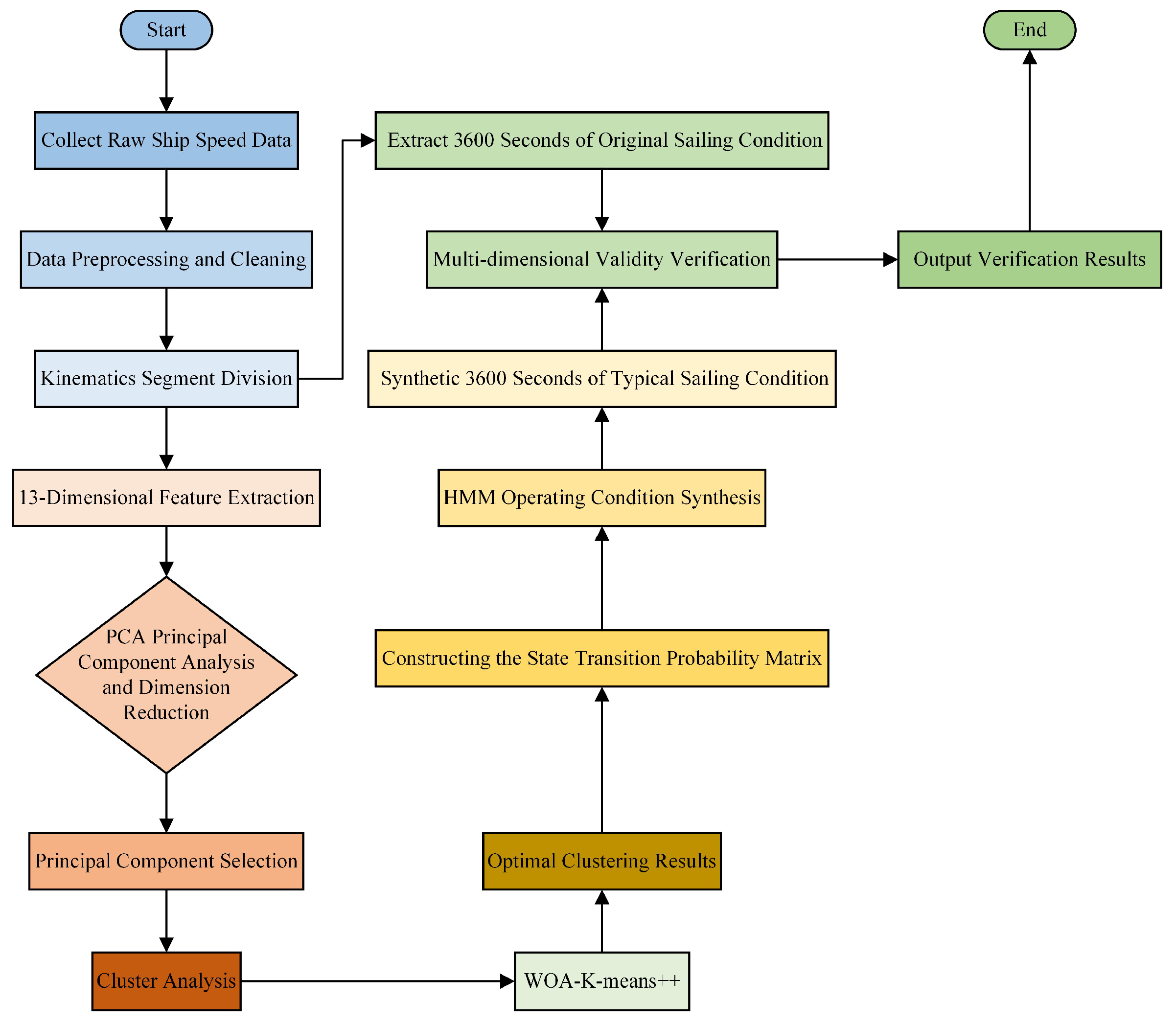
This study proposes a systematic framework integrating data processing, feature dimensionality reduction, state clustering, and temporal sequence synthesis to construct a typical sailing condition for harbor tugs. Figure 3 illustrates the complete technical workflow, from the collection of original ship speed data to the generation and validation of the typical condition. Specifically, the process begins with the acquisition and processing of the original sailing condition data, which is then segmented into kinematic fragments. Subsequently, multi-dimensional feature parameters are extracted from these fragments. To eliminate feature redundancy and enhance computational efficiency, PCA is employed for feature dimensionality reduction. Addressing the limitations of traditional clustering methods regarding initial center selection and global optimization, the WOA is introduced to optimize the initial cluster centers for the K-means++ algorithm, thereby constructing a hybrid WOA-K-means++ clustering model. This model achieves precise classification of the kinematic fragments. Based on this, the typical condition clusters obtained are defined as the hidden states of an HMM. A state transition probability matrix is constructed by analyzing the statistical patterns of state transitions, which is then used to synthesize a representative typical sailing condition profile. Finally, a multi-dimensional validation framework is established to systematically evaluate the synthesized condition. This evaluation assesses its effectiveness in representing the authentic operational patterns of harbor tugs from the perspectives of statistical characteristics, temporal correlations, and probability distributions.

2.3. Data Processing and Kinematic Segment Segmentation

The data for this study was sourced from the ship-borne AIS and voyage data recorder of 16 in-service harbor tugs of the same type at Dalian Port from October to November 2025. The data encompassed various typical operational tasks performed by this type of harbor tug in a busy port environment, including assisting large container ships and oil tankers in berthing and unberthing, in-port maneuvering, waiting at anchorages, and short-distance navigation. The recorded tasks covered all typical duties of this type of harbor tug at Dalian Port, thus the constructed operational profile could reflect the general operational mode of this type of tug in the port, ensuring the diversity and representativeness of the dataset. The data collection period covered both working days and weekends, including different weather conditions (sunny, windy), thus it was representative in both the temporal dimension and common environmental conditions. The raw data was sampled at a frequency of 1 Hz and included information such as timestamps, ground speed, and latitude and longitude coordinates. Due to factors such as signal interference and transmission delays, the raw data often contained noise, missing values, and outliers, necessitating rigorous preprocessing. The data for this study was sourced from the ship-borne AIS and voyage data recorder of 16 in-service port tugs of the same type at Dalian Port from October to November 2025. The data encompassed various typical operational tasks performed by this type of tug in a busy port environment, including assisting large container ships and oil tankers in berthing and unberthing, in-port maneuvering, waiting at anchorages, and short-distance navigation. The recorded tasks covered all typical duties of this type of tug at Dalian Port, thus the constructed operational profile could reflect the general operational mode of this type of tug in the port, ensuring the diversity and representativeness of the dataset. The data collection period covered both working days and weekends, including different weather conditions (sunny, windy), thus it was representative in both the temporal dimension and common environmental conditions. The raw data was sampled at a frequency of 1 Hz and included information such as timestamps, ground speed, and latitude and longitude coordinates. Due to factors such as signal interference and transmission delays, the raw data often contained noise, missing values, and outliers, necessitating rigorous preprocessing.

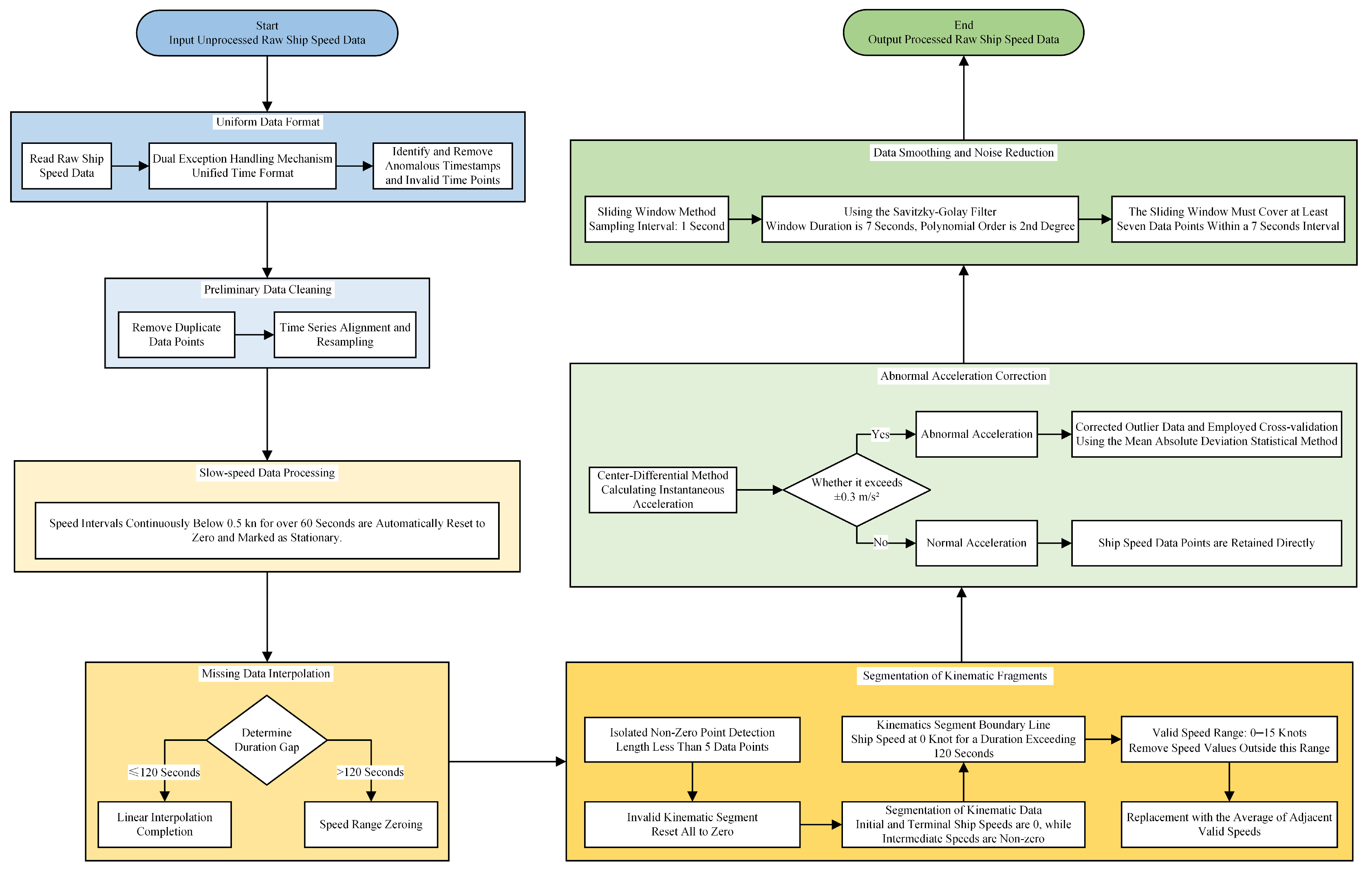
Figure 4 provides a detailed illustration of the “Data Processing and Cleaning” step from the technical workflow shown in Figure 3. It describes the key stages involved in transforming the original sailing condition data into standardized data suitable for subsequent condition construction and analysis:

(1)

Data Format Standardization: The raw ship speed data are read, and a dual-level exception-handling mechanism is employed to parse various time string formats and unify them into a standardized “datetime” format. Subsequently, abnormal timestamps and invalid time points are identified and removed.

(2)

Preliminary Data Cleaning: First, data points corresponding to duplicate timestamps are removed to ensure the uniqueness of the time series. Then, a moving average filter is applied to smooth the data, suppress noise, and remove spikes while preserving the underlying trend. Finally, time series alignment and resampling are performed. Linear interpolation is used to convert non-uniformly spaced data into a strictly regular 1 s interval sequence, providing temporal consistency and a continuous time reference for subsequent feature extraction.

(3)

Low-Speed Data Processing: To focus on sailing behavior, prolonged idle periods (where speed is near zero) that may occur while the harbor tug awaits its next task are processed. Intervals where the speed remains continuously below 0.5 knots for more than 60 s are defined as stationary states. The threshold of 0.5 knots is selected based on typical maneuvering speeds near berths and aligns with AIS data filtering practices in port studies [32]. The 60 s duration ensures that brief operational pauses are not incorrectly classified as idle. The speed values within these intervals are automatically set to zero and flagged accordingly.

(4)

Missing Data Imputation: Different strategies are applied based on the duration of missing data. For gaps longer than 120 s, the corresponding segment is filled with zeros. For gaps of 120 s or less, linear interpolation is used for imputation to maintain the continuity of the speed trend.

(5)

Kinematic Segment Segmentation: The continuous voyage data are partitioned into independent kinematic segments using a “zero-speed cutting method.” A complete kinematic segment is defined as a process starting from zero speed, followed by a period of sailing, and ending when the speed returns to zero. Specific steps include: identifying isolated non-zero points lasting fewer than 5 data points as invalid fragments and setting them to zero; segmenting voyages where both the starting and ending speeds are 0 knots with non-zero speeds in between into independent kinematic segments; and using zero-speed intervals lasting more than 120 s as boundaries between different segments. The 120 s threshold is chosen to distinguish between intentional operational stops and transient pauses during complex maneuvers, a criterion supported by analyses of tug operational patterns [33]. Based on the technical specifications listed in Table 2, the effective speed range for this study is set at 0–15 knots. Values outside this range are considered artifacts from signal jumps or measurement errors and are replaced with the average of the preceding and following valid speed values.

(6)

Abnormal Acceleration Correction: The instantaneous acceleration between consecutive data points within each kinematic segment is calculated using the central difference method. An acceleration threshold of ±0.3 m/s² is set. This threshold is derived from the statistical distribution of acceleration in the dataset (covering 95% of observations) and is consistent with physical limits for tug acceleration during assisted operations, as discussed in prior studies [34]. Data points exceeding this threshold are identified as having abnormal acceleration and are corrected to fall within the threshold range, with cross-validation performed using the mean absolute deviation statistic. Data points with acceleration within the threshold are retained.

(7)

Data Smoothing and Denoising: To eliminate high-frequency noise while preserving key operational features, the ship speed data undergo further smoothing using a Savitzky–Golay filter after outlier treatment. Based on a 1 s sampling period and a 7-point sliding window, this method employs second-order polynomial fitting to reduce noise while maintaining the local extremum characteristics of acceleration changes. Its performance is superior to traditional moving average methods, and limiting the polynomial order helps avoid overfitting.

To ensure the robustness of the chosen segmentation thresholds (stationary speed: 0.5 knots, stationary duration: 60 s, segment separation interval: 120 s), a sensitivity analysis was conducted. We systematically varied these thresholds (±20%) and observed the resulting changes in the number of generated kinematic segments. The results showed that within reasonable variation ranges, the total number of segments fluctuated by less than 5%, and key statistical characteristics (e.g., average segment duration, speed distribution) remained stable. Furthermore, clustering ($K=6$) performed on segments generated using these varied thresholds yielded silhouette coefficient changes of less than 0.03. This demonstrates that the selected thresholds are robust for data segmentation and subsequent analysis, and minor adjustments do not substantially impact the outcomes of the overall methodology.

2.4. Feature Extraction and PCA Dimension Reduction

2.4.1. Feature Extraction

The selection of kinematic segment features directly impacts the accuracy of condition construction. To quantify the sailing characteristics of each segment, this study—based on an analysis of the operational patterns of harbor tugs and with reference to relevant standards for vehicle driving cycle construction both domestically and internationally—extracted a total of 13 features from the speed-time series of the original sailing condition data, categorized into 4 major types. These features constitute a feature matrix that characterizes the multi-dimensional attributes of the kinematic segments [35,36]. The selected 13 features cover key kinematic dimensions such as speed, acceleration, and time proportions, enabling a comprehensive representation of sailing behavior. Analysis of the discriminative power of each feature for the clustering results is provided in Appendix A. Among these, the speed-related features include:

Average Speed, denoted as $v_{avg}$ and measured in knots (kn), which represents the mean speed within a kinematic segment and reflects the overall operating speed level.

$$v_{avg}={\displaystyle \frac{1}{n}}{\sum }_{i=1}^n{v}_i,$$

(1)

where $n$ is the number of data points within the kinematic segment, and $v_i$ is the $i\text{-}\mathrm{t}\mathrm{h}$ speed value.

Maximum Speed, denoted as $v_{max}$ and measured in knots (kn), which represents the maximum speed within a kinematic segment and reflects the operating intensity.

$$v_{max}=\max \{v_1,v_2,\dots ,v_n\},$$

(2)

Speed Standard Deviation, denoted as $v_{std}$ and measured in knots (kn), which represents the standard deviation of the speed series within a kinematic segment and reflects the degree of speed fluctuation.

$$v_{std}=\sqrt{{\displaystyle \frac{1}{n}}{\sum }_{i=1}^n(v_i-v_{avg}{)}^2},$$

(3)

Acceleration features include:

Maximum Acceleration, denoted as $a_{max}$ and measured in m/s², which represents the maximum positive value of the rate of speed change within a kinematic segment and reflects the acceleration capability.

$$a_{max}=\max \{a_i|a_i>0\},$$

(4)

where $a_i$ is the $i\text{-}\mathrm{t}\mathrm{h}$ acceleration value.

Average Acceleration, denoted as $a_{avg}$ and measured in m/s², which represents the mean value of positive acceleration within a kinematic segment and reflects the average acceleration intensity.

$$a_{avg}={\displaystyle \frac{1}{m^{+}}}{\sum }_{a_i>0}{a}_i,$$

(5)

where $m^{+}$ is the number of positive acceleration instances.

Acceleration Standard Deviation, denoted as $a_{std}$ and measured in m/s², which represents the standard deviation of the acceleration series within a kinematic segment and reflects the degree of acceleration fluctuation.

$$a_{std}=\sqrt{{\displaystyle \frac{1}{m^{+}}}{\sum }_{i=1}^{m^{+}}(a_i-a_{avg}{)}^2},$$

(6)

Deceleration features include:

Maximum Deceleration, denoted as $d_{max}$ and measured in m/s², which represents the minimum negative value (i.e., the maximum absolute value of negative acceleration) of the rate of speed change within a kinematic segment and reflects the braking capability.

$$d_{max}=\min \{a_i|a_i<0\},$$

(7)

Average Deceleration, denoted as $d_{avg}$ and measured in m/s², which represents the mean value of negative acceleration within a kinematic segment and reflects the average braking intensity.

$$d_{avg}={\displaystyle \frac{1}{m^{-}}}{\sum }_{a_i<0}{a}_i,$$

(8)

where $m^{-}$ is the number of negative acceleration instances.

Deceleration Standard Deviation, denoted as $d_{std}$ and measured in m/s², which represents the standard deviation of the deceleration series within a kinematic segment and reflects the degree of deceleration fluctuation.

$$d_{std}=\sqrt{{\displaystyle \frac{1}{m^{-}}}{\sum }_{a_i<0}^{m^{-}}(a_i-d_{avg}{)}^2},$$

(9)

Time proportion features include:

Acceleration Time Ratio (percentage of time with $v\ge 0.5$ kn and $a>0.05$ m/s²), denoted as $R_{acc}$ with unit %, which represents the proportion of time where acceleration exceeds the threshold within a kinematic segment, reflecting the frequency of acceleration operations.

$$R_{acc}={\displaystyle \frac{T_{\mathit{acc}}}{T_{\mathit{total}}}},$$

(10)

where $T_{\mathit{acc}}$ is the total acceleration duration, and $T_{\mathit{total}}$ is the total duration of the kinematic segment.

Deceleration Time Ratio (percentage of time with $v\ge 0.5$ kn and $a<-0.05$ m/s², denoted as $R_{dec}$ with unit %, which represents the proportion of time where acceleration is below the negative threshold within a kinematic segment, reflecting the frequency of deceleration operations.

$$R_{dec}={\displaystyle \frac{T_{\mathit{dec}}}{T_{\mathit{total}}}},$$

(11)

where $T_{\mathit{dec}}$ is the total deceleration duration.

Constant Speed Time Ratio (percentage of time with $v\ge 0.5$ kn and $|a|\le 0.05$ m/s², denoted as $R_{con}$ with unit %, which represents the proportion of time where the absolute rate of speed change is below the threshold within a kinematic segment, reflecting the degree of stable operation.

$$R_{con}={\displaystyle \frac{T_{\mathit{con}}}{T_{\mathit{total}}}},$$

(12)

where $T_{\mathit{con}}$ is the total constant speed duration.

Idle Time Ratio (percentage of time with $v<0.5$ kn, denoted as $R_{idle}$ with unit %, which represents the proportion of time where speed is close to zero within a kinematic segment, reflecting the waiting or preparation time.

$$R_{idle}={\displaystyle \frac{T_{\mathit{idle}}}{T_{\mathit{total}}}},$$

(13)

where $T_{\mathit{idle}}$ is the total idle duration.

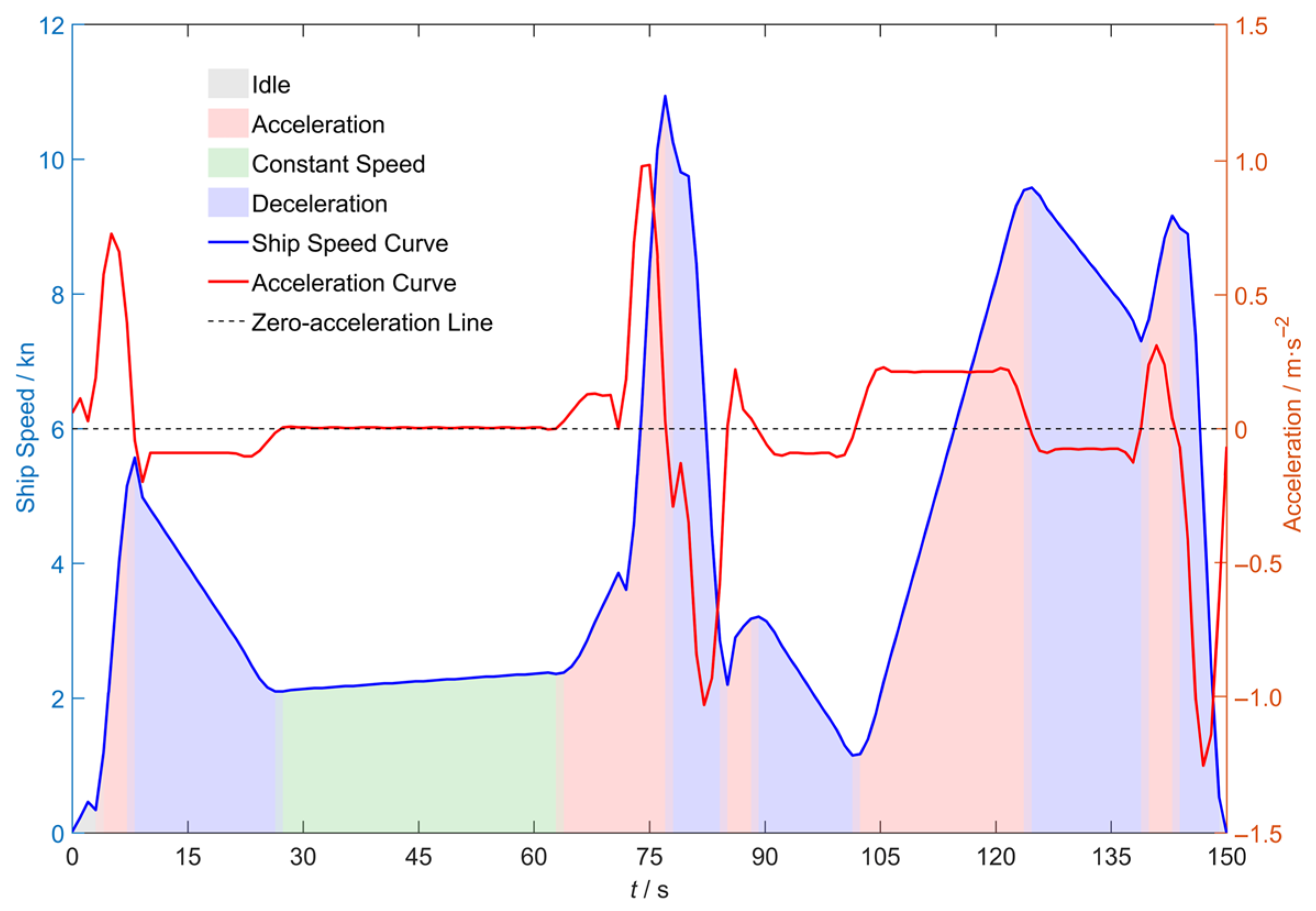
Figure 5 presents a representative ship speed kinematic segment and provides a micro-state analysis. As shown, the continuous speed curve is decomposed and annotated into four fundamental kinematic state phases: “Idle,” “Acceleration,” “Cruise,” and “Deceleration.” To more intuitively visualize the dynamic changes in ship speed, the corresponding acceleration curve is plotted synchronously in the figure. This figure clearly demonstrates that a typical kinematic segment is not a single motion state but rather a sequence composed of the aforementioned basic states arranged in a specific temporal order. For example, a complete operational cycle may start from “Idle,” proceed through “Acceleration” to reach a target speed, maintain a “Cruise” state to execute a task, and finally return to an “Idle” state via “Deceleration.” The significance of this analysis lies in revealing the microscopic dynamic structure of ship motion, thereby clarifying the intrinsic reasons for the differences between various clustered kinematic segments.

2.4.2. PCA Dimension Reduction

PCA is a multivariate linear dimensionality reduction method based on statistical characteristics. It captures commonalities among features by extracting the principal directions of data variation, thereby revealing the data structure and achieving dimension compression. The core objective of PCA is to transform a set of potentially correlated variables into linearly uncorrelated principal components through orthogonal transformation, with each principal component ranked in descending order of its variance. This method can significantly reduce dimensionality while retaining most of the information from the original data [37]. In the feature analysis for harbor tug operational conditions, although the 13 features selected in this study comprehensively describe ship speed behavior, the correlations among them can easily lead to the curse of dimensionality and multicollinearity issues. Therefore, it is necessary to perform PCA for dimensionality reduction. To assess the relevance of each feature for distinguishing operational modes, a preliminary analysis of variance (ANOVA) was conducted across the six identified clusters (see Appendix A). Features such as average speed ($v_{avg}$), idle time ratio ($R_{idle}$), and constant speed time ratio ($R_{con}$) showed high F-statistics, confirming their discriminative power. This study implemented PCA based on the standardized 13-dimensional features and their correlation coefficient matrix, subsequently screening for representative principal components.

Since the physical dimensions of each feature differ and their numerical ranges vary significantly, direct use in cluster analysis would allow features with larger numerical values to dominate the distance calculations, thereby obscuring the contribution of features with smaller values. To address this, the Z-score normalization method was first applied to transform the original feature matrix into a dimensionless space with a mean of 0 and a standard deviation of 1. This eliminates the influence of differing units and establishes a foundation for subsequent dimensionality reduction and cluster analysis.

The normalization formula is:

$$z={\displaystyle \frac{x- \mu }{\sigma }},$$

(14)

where $\mu$ is the mean of the feature, and $\sigma$ is the standard deviation of the feature.

The specific mathematical derivation process for PCA dimensionality reduction is as follows:

First, let the standardized original feature matrix be ${\mathit{X}}_{n\times p}$, where n is the number of samples (i.e., kinematic segments) and p is the number of variables (13 features).

$$\mathit{X}=\left[X_1,X_2\dots \dots ,X_n\right]=\left[\begin{array}{cccc}{x}_{11}& x_{12}& \dots & x_{1p}\\ x_{21}& x_{22}& \dots & x_{2p}\\ ⋮& ⋮& ⋮& ⋮\\ x_{n1}& x_{n2}& \dots & x_{np}\end{array}\right],$$

(15)

The correlation coefficient matrix R of the standardized original feature matrix X is:

$$\mathit{R}=\left[\begin{array}{cccc}{r}_{11}& r_{12}& \dots & r_{1m}\\ r_{21}& r_{22}& \dots & r_{2m}\\ ⋮& ⋮& \ddots & ⋮\\ r_{n1}& r_{n2}& \dots & r_{nm}\end{array}\right],$$

(16)

where the calculation formula for $r_{ij}$ is:

$$r_{ij}={\displaystyle \frac{{\sum }_{k=1}^n(x_{ki}-{\overline{u}}_i)(x_{kj}-{\overline{u}}_j)}{\sqrt{{\sum }_{k=1}^n(x_{ki}-{\overline{u}}_i{)}^2{\sum }_{k=1}^n(x_{kj}-{\overline{u}}_j{)}^2}}},$$

(17)

The covariance matrix calculation formula is:

$$Cov(\mathit{X})={\displaystyle \frac{1}{n-1}}{\mathit{X}}^T\mathit{X},$$

(18)

The covariance matrix is a $p\times p$ symmetric matrix. The diagonal elements are the variances of each feature, and the off-diagonal elements are the covariances between features, reflecting the strength of the linear relationships among them.

The goal of PCA dimensionality reduction is to find a principal component matrix ${\mathit{Z}}_{n\times k}$ (where $k\le p$) such that:

• Each principal component is a linear combination of the original features: $Z_j=a_{1j}{X}_1+a_{2j}{X}_2+\cdots +a_{pj}{X}_p$;
• The principal components are uncorrelated with each other: $Cov(Z_i,Z_j)=0$ when $i\ne j$;
• The principal components are arranged in order of decreasing variance: $Var\left(Z_1\right)\ge Var\left(Z_2\right)\ge \cdots \ge Var\left(Z_p\right)$.

By solving the characteristic equation $|Cov(\mathit{Z})- \lambda I|=0$, 13 eigenvalues ${\lambda }_i$ and their corresponding eigenvectors $v_i$ are obtained. The eigenvalue ${\lambda }_i$ represents the variance of the $i\text{-}\mathrm{t}\mathrm{h}$ principal component, and the components of the eigenvector $v_i$ indicate the weights of the original features in that principal component. Mathematically, this is equivalent to performing spectral decomposition on the covariance matrix:

$$Cov\left(\mathit{Z}\right)=V\Lambda V^T,$$

(19)

where $V$ is an orthogonal matrix and $\Lambda$ is a diagonal matrix.

The formula for calculating the contribution rate of a principal component is:

$$C{R}_i={\displaystyle \frac{{\lambda }_i}{{\sum }_{j=1}^{13} {\lambda }_j}}\times 100\%,$$

(20)

where ${CR}_i$ is the contribution rate of the $i\text{-}\mathrm{t}\mathrm{h}$ principal component, representing the amount of original information carried by this component.

The cumulative contribution rate of the first $k$ principal components is:

$$CC{R}_k={\displaystyle \frac{{\sum }_{j=1}^k {\lambda }_j}{{\sum }_{j=1}^{13} {\lambda }_j}}\times 100\%,$$

(21)

In practical applications, the first few principal components whose cumulative contribution rate reaches above 85% are typically selected to retain most of the original information while achieving dimensionality reduction.

Principal Component Scores and Loadings Calculation:

The principal component scores represent the coordinates of each sample in the new principal component coordinate system. The calculation formula is:

$$\mathit{S}=\mathit{X}\mathit{V},$$

(22)

where $\mathit{S}$ is the principal component score matrix, $\mathit{X}$ is the standardized original data matrix, and $\mathit{V}$ is the eigenvector matrix.

The principal component loadings represent the correlation between the original features and the principal components. The calculation formula is:

$$\mathit{L}=\mathit{V}\sqrt{\mathit{\Lambda }},$$

(23)

where $\mathit{\Lambda }=diag({\lambda }_1, {\lambda }_2,\dots , {\lambda }_{13})$. The element $l_{ij}$ of the loading matrix $\mathit{L}$ indicates the correlation coefficient between the $i\text{-}\mathrm{t}\mathrm{h}$ original feature and the $j\text{-}\mathrm{t}\mathrm{h}$ principal component.

2.5. Kinematic Segment Clustering

2.5.1. Traditional Clustering Algorithms

The K-means algorithm is a classic partition-based clustering method. Its fundamental principle is to iteratively partition data into K clusters, aiming to maximize intra-cluster similarity and inter-cluster dissimilarity. This algorithm is widely used in cluster analysis due to its simplicity, computational efficiency, and strong interpretability. However, the traditional K-means algorithm randomly initializes cluster centers, and different initial values can easily cause the algorithm to converge to different local optima, resulting in poor stability and low repeatability of clustering outcomes. Furthermore, the objective function of the K-means algorithm is to minimize the squared sum of squared errors (SSEs) within clusters. This makes the calculation of cluster centers significantly susceptible to interference from isolated outliers [38].

To overcome the limitations of the traditional K-means algorithm, namely its high sensitivity to initial cluster centers and tendency to converge to local optima, the K-means++ algorithm was proposed. Its core improvement lies in optimizing the selection of initial centers using a “D² sampling (Double Sampling)” strategy based on squared distance weighting: the first cluster center is randomly selected, and subsequent centers are chosen iteratively from the remaining data points with a probability proportional to the squared shortest distance to any already chosen center. This strategy helps to spread the initial cluster centers as far apart as possible within the data space, thereby significantly increasing the likelihood of the algorithm converging to a near-global optimum and accelerating the convergence speed. Although it introduces some additional computational overhead, its overall time complexity remains the same as the traditional K-means algorithm due to faster convergence [39]. However, for the high-dimensional, non-convex feature space derived from harbor tug kinematic segments, both K-means and K-means++ face specific challenges. The random initialization of K-means often leads to inconsistent clustering results across multiple runs. While K-means++ improves stability through better initial center sampling, it may still converge to local optima when the cluster structure is complex, resulting in higher within-cluster SSE compared to the proposed hybrid method. Furthermore, these algorithms are sensitive to outliers and feature scaling, which are prevalent in real-world ship data. These limitations motivate the need for a more robust initialization strategy guided by global optimization.

The process of the K-means++ clustering algorithm is as follows:

For a feature dataset $\mathit{X}$:

$$\mathit{X}=\{x_i{\}}_{i=1}^M\subset {\mathbb{R}}^d,$$

(24)

where $\mathit{X}$ is the feature dataset matrix; $x_i$ is the feature vector of the $i\text{-}\mathrm{t}\mathrm{h}$ sample; $M$ is the total number of samples; and $d$ is the feature dimensionality.

The K-means++ initialization process is as follows:

(1) Randomly select the first cluster center:

$$c_1=x_r,\hspace{0.33em}r~U\{1,M\},$$

(25)

where $c_j$ is the $j\text{-}\mathrm{t}\mathrm{h}$ cluster center; $\mathrm{K}$ is the number of clusters; and $U\{1,M\}$ denotes a uniform distribution from 1 to $M$.

(2) For $k=2,\dots ,\mathrm{K}$, calculate the shortest distance from each sample to the existing centers:

$$D\left(x_i\right)={\mathrm{m}\mathrm{i}\mathrm{n}}_{j=1}^{k-1}\Vert x_i-c_j{\Vert }^2,$$

(26)

(3) Select the next center with probability $p_i$:

$$p_i={\displaystyle \frac{D\left(x_i\right)}{{\sum }_{j=1}^{M}D\left(x_j\right)}},$$

(27)

(4) Repeat step 3 until $\mathrm{K}$ initial centers are selected.

Using the intra-cluster distance SSE as the fitness function:

$$\mathrm{Fitness}={\sum }_{k=1}^K{\sum }_{x_i\in C_k}\Vert x_i-c_k{\Vert }^2,$$

(28)

where $c_k$ is the $k\text{-}\mathrm{t}\mathrm{h}$ cluster and $c_k$ is its center.

The expected upper bound for the error of K-means++ is:

$$\mathbb{E}\left[J\right]\le 8(\mathit{ln}k+2)J_{opt},$$

(29)

where $J_{opt}$ is the objective function value of the global optimal solution. This theoretical guarantee indicates that K-means++ has better performance compared to random initialization.

2.5.2. WOA-K-Means++ Clustering Algorithm

Since the K-means++ clustering algorithm still cannot guarantee obtaining the global optimum, and its D² sampling mechanism may tend to select outliers as initial cluster centers, thereby affecting the final clustering quality, this study proposes a hybrid clustering algorithm (WOA-K-means++) that integrates WOA with K-means++. This algorithm adopts a strategy of “global optimization + local fine-tuning,” incorporating the global search capability of WOA, a robust processing mechanism for outliers, and a stability optimization strategy based on multiple runs to systematically enhance clustering performance. Specifically, the algorithm first leverages the powerful global optimization capability of the WOA, which mimics the bubble-net hunting behavior of humpback whales, to efficiently search the solution space for an initial combination of cluster centers that is closer to the true cluster structure. Subsequently, this optimal combination is used as the initial input for the K-means++ algorithm to achieve rapid local convergence. To address the issue of sensitivity to outliers, the algorithm incorporates outlier detection during the initialization phase. Potential outliers are assigned lower weights or temporarily excluded from the candidate center set based on distance or density measures, ensuring that the D2 sampling focuses on the main distribution of the data. Regarding stability, the algorithm executes multiple independent clustering processes and uses the silhouette coefficient as the core evaluation metric, replacing the traditional criterion of minimizing intra-cluster SSE. The clustering result with the highest average silhouette coefficient is ultimately selected as the output. This method simultaneously considers intra-cluster compactness and inter-cluster separation, enabling the acquisition of more stable and balanced clustering solutions. Experimental results show that WOA-K-means++ outperforms the traditional K-means++ algorithm in terms of convergence speed, clustering accuracy, and handling high-dimensional, non-convex datasets.

Parameter Settings and Sensitivity: The WOA parameters were set as follows: $population size=50$, $maximum iterations=100$, a linearly decreasing from 2 to 0, and spiral constant $b=1$. These values are commonly adopted in WOA literature and were found to provide a balance between exploration and exploitation in preliminary trials [40]. The spiral constant b controls the shape of the spiral update during bubble-net attacking; a value of 1 is the standard setting, effectively balancing search scope and precision. A sensitivity analysis (see Appendix B) showed that the algorithm’s performance is robust to moderate variations in these parameters. To evaluate the sensitivity of key WOA parameters (population size, maximum iterations, spiral constant b) on the final clustering performance (measured by the silhouette coefficient), a parameter scan experiment was conducted. The results show that when parameters varied moderately around the baseline ($population size=50$, $max iterations=100$, $b=1$), the fluctuation in clustering performance was minimal ($standard deviation of silhouette coefficient<0.02$), indicating that the algorithm is robust and not sensitive to such parameter variations. Detailed results are provided in Appendix B.

Computational Complexity and Scalability: The time complexity of WOA-K-means++ is $O(N·I·K·d)$, where $N$ is the population size, $I$ is the number of iterations, $K$ is cluster count, and $d$ is dimensionality. While higher than K-means++ due to the population-based search, the total runtime remains acceptable for offline condition construction (7.85 s average in our experiments, Table 5). The method scales linearly with data size and is suitable for typical harbor tug datasets comprising thousands of kinematic segments. For real-time applications, the trained HMM can be used for rapid state sequence generation without re-clustering.

The WOA is a population-based metaheuristic optimization algorithm proposed by Mirjalili and Lewis in 2016 [41]. Inspired by the unique spiral bubble-net hunting strategy of humpback whales, it primarily consists of three phases: encircling prey, bubble-net attacking, and searching for prey [42]. Compared to traditional optimization algorithms such as PSO [43] and GA [44], WOA offers advantages including a simple structure, few parameters requiring adjustment, strong global search capability, fast convergence speed, and ease of escaping local optima.

The WOA process is as follows:

(1) Encircling Prey Phase:

Whales update their positions to approach the prey using the following formulas:

$$\overrightarrow{D}=|\overrightarrow{C}\cdot {\overrightarrow{X}}^{\left(t\right)}-\overrightarrow{X}(t)|,$$

(30)

$$\overrightarrow{X}(t+1)={\overrightarrow{X}}^{(t)}-\overrightarrow{A}\cdot \overrightarrow{D},$$

(31)

where ${\overrightarrow{X}}^{(t)}$ represents the position of the current best solution; $\overrightarrow{A}$ and $\overrightarrow{C}$ are coefficient vectors, and $\overrightarrow{A}=2\overrightarrow{a}\cdot \overrightarrow{r}-\overrightarrow{a}$, $\overrightarrow{C}=2\cdot \overrightarrow{r}$, with $\overrightarrow{a}$ decreasing linearly from 2 to 0 over iterations, and $\overrightarrow{r}$ is a random vector in [0, 1].

(2) Bubble-net Attacking Phase (Spiral Updating Position):

Whales move towards the prey in a spiral manner:

$$\overrightarrow{X}(t+1)={\overrightarrow{D}}^{\prime }\cdot e^{bl}\cdot \cos (2\pi l)+{\overrightarrow{X}}^{(t)},$$

(32)

where ${\overrightarrow{D}}^{\prime }=\left|{\overrightarrow{X}}^{(t)}-\overrightarrow{X}(t)\right|$ represents the distance between the current individual and the best solution; $b$ is a constant defining the spiral shape (typically set to 1); and $l$ is a random number in [−1, 1].

(3) Searching for Prey Phase:

When $|\overrightarrow{A}|>1$, whales perform a global search:

$$\overrightarrow{X}(t+1)={\overrightarrow{X}}_{rand}-\overrightarrow{A}\cdot \overrightarrow{D},$$

(33)

where ${\overrightarrow{X}}_{rand}$ is the position of a randomly selected whale.

The WOA-K-means++ Clustering Algorithm Process:

(1) Encoding and Initialization:

Each whale individual is encoded as a set of cluster centers. The population size is set to 50, and the maximum number of iterations is 100.

$$Whal{e}_i=\left[c_{i1},c_{i2},\dots ,c_{ik,}\right],c_{ij}\in R^d,$$

(34)

where $c_{ij}$ represents the $j\text{-}\mathrm{t}\mathrm{h}$ cluster center of the $i\text{-}th$ whale, $d$ is the data dimension, and $k$ is the number of clusters.

(2) Fitness Function Design:

The K-means++ objective function (intra-cluster distance SSE) is used as the fitness function:

$$Fitness=SSE={{\sum }_{k=1}^K{\sum }_{x\in C_k}‖x-c_k‖}^2,$$

(35)

The optimization goal is to minimize the fitness function value.

(3) WOA Optimization Process:

In each generation, for each individual in the whale population (i.e., a proposed set of cluster centers):

(a) Assignment Step: Assign all sample points to their nearest cluster center, forming K clusters.

(b) Update Step: Recalculate the mean of all sample points in each cluster as the new center for that cluster.

The SSE is calculated based on the new centers, yielding the fitness value for that individual.

The whale population updates its positions (i.e., generates new combinations of cluster centers) according to the WOA’s encircling, spiral attacking, or random search strategies, proceeding to the next generation. The “assignment-update” operation performed for each candidate solution is essentially one standard K-means++ iteration, aimed at quickly assessing the quality of that set of center points. Here, WOA plays the role of a global searcher for the optimal initial centers, replacing the probability-based initialization strategy in K-means++.

(4) Optimal Solution Output and Final Clustering: After the WOA iterations conclude, the individual with the minimum fitness is output as the optimal set of initial cluster centers. Subsequently, starting from this optimized set of centers, a complete standard K-means++ algorithm is run for multiple iterations until cluster assignments no longer change, yielding the final stable clustering result.

(5) Determination of the Number of Clusters (K): The optimal K value is determined using a combined approach of the elbow method and the silhouette coefficient. The aforementioned WOA-K-means++ process is used for evaluating different K values.

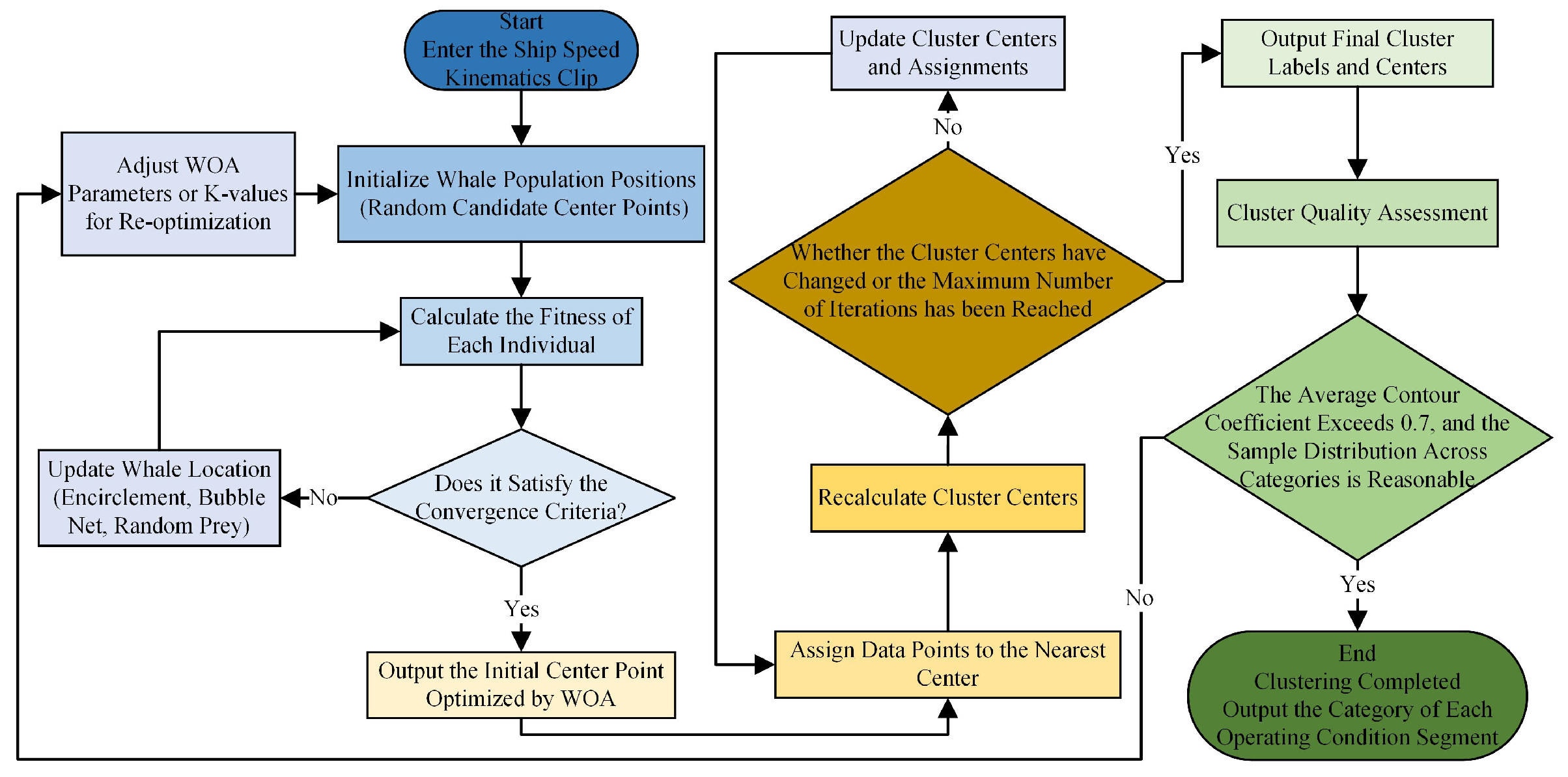
All algorithms were implemented and run using Python 3.9 on a computer with an Intel Core i7-12700H processor and 32GB RAM. Key libraries included NumPy, SciPy, scikit-learn, and hmmlearn. Figure 6 illustrates the kinematic segment clustering workflow based on WOA-K-means++.

2.6. Sailing Condition Construction Based on HMM

The essence of clustering algorithms is to “slice” the time series and identify several static operational modes. However, this process discards all information regarding the sequence and duration of these modes. To construct a dynamic, simulation-ready typical sailing condition, a shift from “mode identification” to “sequence modeling” is essential. An HMM is a probabilistic statistical model used to describe a sequence of observations generated by a hidden Markov chain. It is particularly well-suited for modeling and analyzing dynamic processes with temporal dependencies and state transition characteristics [45]. In the context of sailing condition construction, the HMM treats the continuous kinematic segments as observable outputs while abstracting the underlying different operational modes into hidden states, thereby revealing the intrinsic structure of the sailing data. For the task of synthesizing a typical sailing condition, the HMM can simulate not only the proportion of various conditions but, more importantly, the dynamic logic governing the transitions between them.

A classical HMM is typically parameterized by the following five elements, denoted as $\lambda =(N,M,A,B,\pi )$:

(1)

State Set $\mathit{S}=\{S_1,S_2,\dots ,S_N\}$, where N is the number of hidden states in the model. In this study, each state corresponds to a type of sailing condition. In this study, each hidden state corresponds directly to one of the sailing condition clusters (C1–C6, see Table 7) identified by WOA-K-means++, representing six operationally meaningful modes: Idle/Fine-tuning (C1), Low-speed Harbor Maneuvering (C2), Medium-low Speed Cruising (C3), Medium-high Speed Towing (C4), High-speed Sailing (C5), and Full-speed/Emergency (C6).

(2)

Observation Set $\mathit{V}=\{v_1,v_2,\dots ,v_M\}$, where M is the number of discrete observation symbols. For continuous sailing data (e.g., speed, acceleration), modeling is usually performed via vector quantization or continuous probability density functions.

(3)

State Transition Probability Matrix $\mathit{A}={\left[a_{ij}\right]}_{N\times N}$, where $a_{ij}=P(q_{t+1}=S_j|q_t=S_i)$, $1\le i$, $j\le N$. This element represents the probability of transitioning from state S_i at time $t$ to state $S_j$ at time $t+1$. The matrix satisfies ${\sum }_{j=1}^N{a}_{ij}=1$.

(4)

Observation Probability Distribution $\mathit{B}=\{b_j(k)\}$. For discrete observations, $b_j(\mathrm{k})=P(o_t=v_k|q_t=S_j)$, $1\le j\le N$, $1\le k\le M$, represents the probability of generating observation symbol $v_k$ while in state $S_j$. For continuous observations, it is often represented by a multivariate Gaussian distribution or a mixture thereof: $b_j(o_t)={\sum }_{m=1}^M{c}_{jm}N(o_t;{\mu }_{jm},{\sum }_{jm})$, where $c_{jm}$ is the mixture weight, and ${\mu }_{jm}$ and ${\sum }_{jm}$ are the mean vector and covariance matrix, respectively.

(5)

Initial State Probability Distribution $\pi =\left\{{\pi }_i\right\}$, where ${\pi }_i=P(q_1=S_i)$, $1\le i\le N$, represents the probability that the model starts in each state at time $t=1$.

HMMs aim to solve three fundamental problems, and their corresponding efficient algorithms form the core of model application:

(1) Evaluation Problem: Given an observation sequence $O=(o_1,o_2,\dots ,o_t)$ and model parameters $\lambda$, compute the probability $P(O|\lambda )$ that this sequence appears. The Forward Algorithm solves this efficiently via dynamic programming. Defining the forward variable ${\alpha }_t\left(i\right)=P\left(o_1,o_2,\dots ,o_t,q_t=S_i|\lambda \right)$, the recursive formulas are:

$${\alpha }_1\left(i\right) ={\pi }_i{b}_i\left(o_1\right),$$

(36)

$${\alpha }_{t+1}\left(j\right)=\left[{\sum }_{i=1}^N{\alpha }_t(i)a_{ij}\right]b_j(o_{t+1}),t=1,2,\dots ,T-1,$$

(37)

Finally, $P(O\mid \lambda )={\sum }_{i=1}^N{\alpha }_T(i)$.

(2) Decoding Problem: Given an observation sequence $O$ and model $\lambda$, find an optimal hidden state sequence $Q \ast =(q_1, q_2,\dots ,q_t)$ that maximizes $P(Q|O, \lambda )$. The Viterbi Algorithm is the standard method for finding the optimal path by maximizing path probability rather than summing. Defining the variable ${\delta }_t(i)={\max }_{q_1,\dots ,q_{t-1}}P(q_1,\dots ,q_t=S_i,o_1,\dots ,o_t|\lambda )$, the recursive process is:

$${\delta }_1(i)={\pi }_i{b}_i(o_i),$$

(38)

$${\delta }_t(j)=\underset{1\le i\le N}{\mathrm{m}\mathrm{a}\mathrm{x}}[{\delta }_{t-1}(i)a_{ij}]\cdot b_j(o_t),$$

(39)

$${\psi }_t(j)=\mathit{arg}\underset{1\le i\le N}{\mathrm{m}\mathrm{a}\mathrm{x}}[{\delta }_{t-1}(i)a_{ij}],$$

(40)

The backtracking pointer ${\psi }_t(j)$ is used to record the optimal path, and the state sequence $Q$* is finally obtained through backtracking.

(3) Learning Problem: Given an observation sequence $O$, adjust the model parameters $\lambda$ to maximize $P(O|\lambda )$. The Baum–Welch Algorithm (a special case of the Expectation-Maximization algorithm for HMMs) solves this through iterative parameter re-estimation. The algorithm uses the forward variable ${\alpha }_t(i)$ and the backward variable ${\beta }_t(i)=P(o_{t+1},\dots ,o_T|q_t=S_i,\lambda )$ to compute two intermediate variables:

$${\xi }_t(i,j)={\displaystyle \frac{{\alpha }_t(i)a_{ij}{b}_j(o_{t+1}){\beta }_{t+1}(j)}{P(O|\lambda )}},$$

(41)

The above represents the probability of being in state $S_i$ at time t and state $S_j$ at time $t+1$, given the observation sequence. Also,

$${\gamma }_t(i)={\sum }_{j=1}^N{\xi }_t(i,j),$$

(42)

The above represents the probability of being in state $S_i$ at time $t$. The model parameters are then iteratively updated until convergence using:

$${\widehat{\pi }}_i={\gamma }_1(i),$$

(43)

$${\widehat{a}}_{ij}={\displaystyle \frac{{\sum }_{t=1}^{T-1}{\xi }_t(i,j)}{{\sum }_{t=1}^{T-1}{\gamma }_t(i)}},$$

(44)

$${\widehat{b}}_j(k)={\displaystyle \frac{{\sum }_{t=1}^T{\gamma }_t(j)\cdot \Phi (o_t=v_k)}{{\sum }_{t=1}^T{\gamma }_t(j)}},$$

(45)

where Φ(∙) is the indicator function. For continuous observations, parameter updates involve re-estimating the Gaussian mixture model parameters.

In this study, to construct a high-quality, high-fidelity typical sailing condition, a complete “Clustering-HMM Modeling-Synthesis” framework was proposed and implemented. First, K-means++ clustering is employed to discretize and encode the high-dimensional kinematic segment features, forming an observation sequence. Subsequently, the Baum–Welch algorithm is applied to learn HMM parameters $\lambda$ that characterize the typical sailing condition behavioral patterns. The learned HMM can not only be used to decode the sailing mode of kinematic segments, revealing their microscopic state transition processes, but also to synthesize a typical sailing condition profile with statistical representativeness and preserved temporal dynamics of the original data by generating observation sequences (through sampling based on the state transition matrix and observation probabilities) that conform to the model’s statistical properties. To concretely implement a continuous typical sailing condition, the following steps are executed based on the HMM: First, the proportion of kinematic segments belonging to each cluster in the original sailing condition data is calculated. A target total duration (3600 s in this study) is set, and the time allocation for segments from each cluster is determined proportionally. Next, the kinematic segments within each cluster are sorted in ascending order of their distance to the respective cluster center. Then, guided by the HMM’s state transition probability matrix, the typical sailing condition is constructed by sequentially selecting the top-ranked segments for concatenation. This continues until the time allocations for all clusters and the total duration are met. The last segment exceeding the target duration is truncated and smoothed for transition. This framework effectively overcomes the shortcomings in temporal rationality inherent in traditional methods based on random segment splicing, providing a solid theoretical foundation for constructing high-quality, high-fidelity standard sailing conditions.

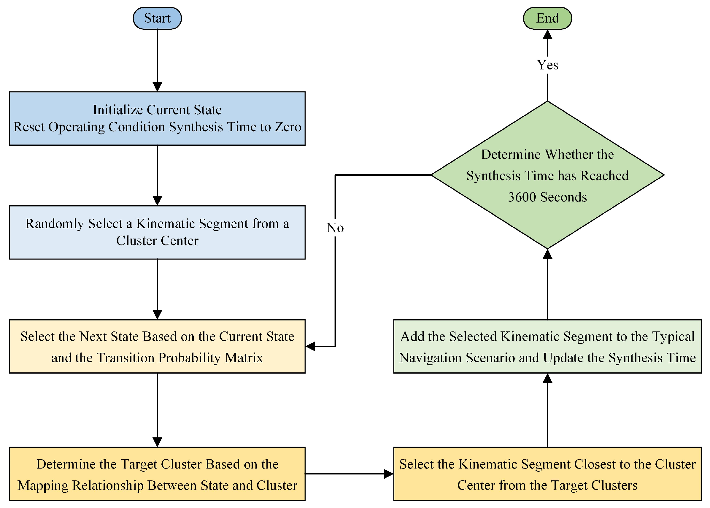
Based on the aforementioned basic principles of HMM, the complete algorithm flow for synthesizing typical navigation conditions in this study is illustrated in Figure 7. The process starts with the input clustering label sequence, learns state transition probabilities through HMM training, synthesizes new state sequences, and finally generates typical profile curves through segment selection and connection. Its core steps include:

(1)

Input preparation: Arrange the labels of all motion segments after WOA-K-means++ clustering in their original temporal order to form an observation state sequence.

(2)

HMM training: Utilizing the Baum–Welch algorithm, the aforementioned state sequence is used as training data to learn and obtain the matrix $\mathit{A}$ that represents the transition rules between states.

(3)

State sequence synthesis: Based on the learned transition matrix $\mathit{A}$ and initial state distribution $\pi$, generate a new hidden state sequence with a total duration of 3600 s through probability sampling.

(4)

Motion clip mapping and stitching: Based on the duration of each state (corresponding to a cluster category) in the synthesized state sequence, the real-world motion clip closest to the center of the corresponding original cluster is selected.

(5)

Smoothing and Output: The selected motion clips are concatenated in the order of the synthetic sequence, and smoothing is applied to the connections. Finally, a continuous speed-time curve under typical navigation conditions is output.

HMM Application Specifics and Assumptions: In this study, the hidden states correspond directly to the six operational condition clusters (C1–C6) identified by WOA-K-means++. The observable output is the kinematic segment label (i.e., cluster ID). We assume a first-order Markov process for state transitions, which is reasonable given that the next operational mode of a tug is largely determined by its current mode and immediate task requirements. The emission probabilities are deterministic—each hidden state (cluster) emits its corresponding cluster ID with probability 1.0. This simplification is valid because the clustering already abstracts each segment into a discrete state. The Baum–Welch algorithm is then used to learn the state transition probability matrix A from the sequence of cluster labels in the historical data. This matrix captures the empirical probability of transitioning from one operational condition to another, encoding the temporal logic of tug operations (e.g., high-speed states rarely persist, deceleration transitions are more direct).

In this study, the HMM was implemented using the Multinomial HMM model from the HMM learn library. The observations were the deterministic cluster labels (1–6). Model training (i.e., learning the state transition matrix $\mathit{A}$) employed the Baum–Welch algorithm with a maximum of 100 iterations and a convergence tolerance of 1 × 10⁻⁴. The initial state probability distribution $\pi$ was estimated from the initial proportions of each category of kinematic segments in the data. After training, the Viterbi algorithm was used to decode the original state sequence for verification. To synthesize a new state sequence, starting from an initial state sampled from $\pi$, the next state was sampled probabilistically according to the learned matrix $\mathit{A}$ until the cumulative duration reached the target (3600 s). Finally, the speed profile of the typical sailing condition was generated by concatenating real kinematic segments closest to their respective cluster centers, selected according to the duration proportion of each state in the synthesized state sequence.

In this study, the specific working process of the HMM involves arranging the kinematic segments from different clusters in chronological order to form a state sequence. The frequency of transitions from state i to state j in this sequence is counted and normalized to obtain a $K\times K$ state transition probability matrix $\mathit{A}$. Based on the actual time series of n kinematic segments, the state transition probability matrix is calculated as:

$$a_{ij}={\displaystyle \frac{N_{ij}}{{\sum }_{k=1}^K{N}_{ik}}},$$

(46)

where $N_{ij}$ is the number of transitions from state $i$ to state $j$. Transitions between different states (i.e., different clusters) are modeled using maximum likelihood estimation. Matrix $\mathit{A}$ characterizes the statistical patterns of transitions between different states.

3. Results and Discussion

3.1. Results of Data Processing and Kinematic Segment Segmentation

Through systematic data processing, 5271 valid kinematic segments were extracted from the raw data. The duration of these segments primarily ranged between 100 and 500 s, consistent with the frequent and dynamic operational characteristics of port tugs. Detailed statistical results from each data processing stage are summarized in

Table 3. Statistics of Data Processing Results.

Processing Type	Data Volume (10k Records)	Proportion (%)	Processing Method
Original Vessel Speed Data	307.5	100.0	-
Missing Data	8.03	2.61	Interpolation/Removal
Speed Anomalies	3.66	1.19	Removal
Acceleration Anomalies	5.04	1.64	Correction
Extended Stops	10.52	3.42	Flagging
Total Valid Data	280.25	91.14	-

. The processed data provides a high-quality foundation for subsequent analysis.

3.2. Results of Feature Extraction and PCA Dimensionality Reduction

3.2.1. Correlation Analysis of Feature Parameters

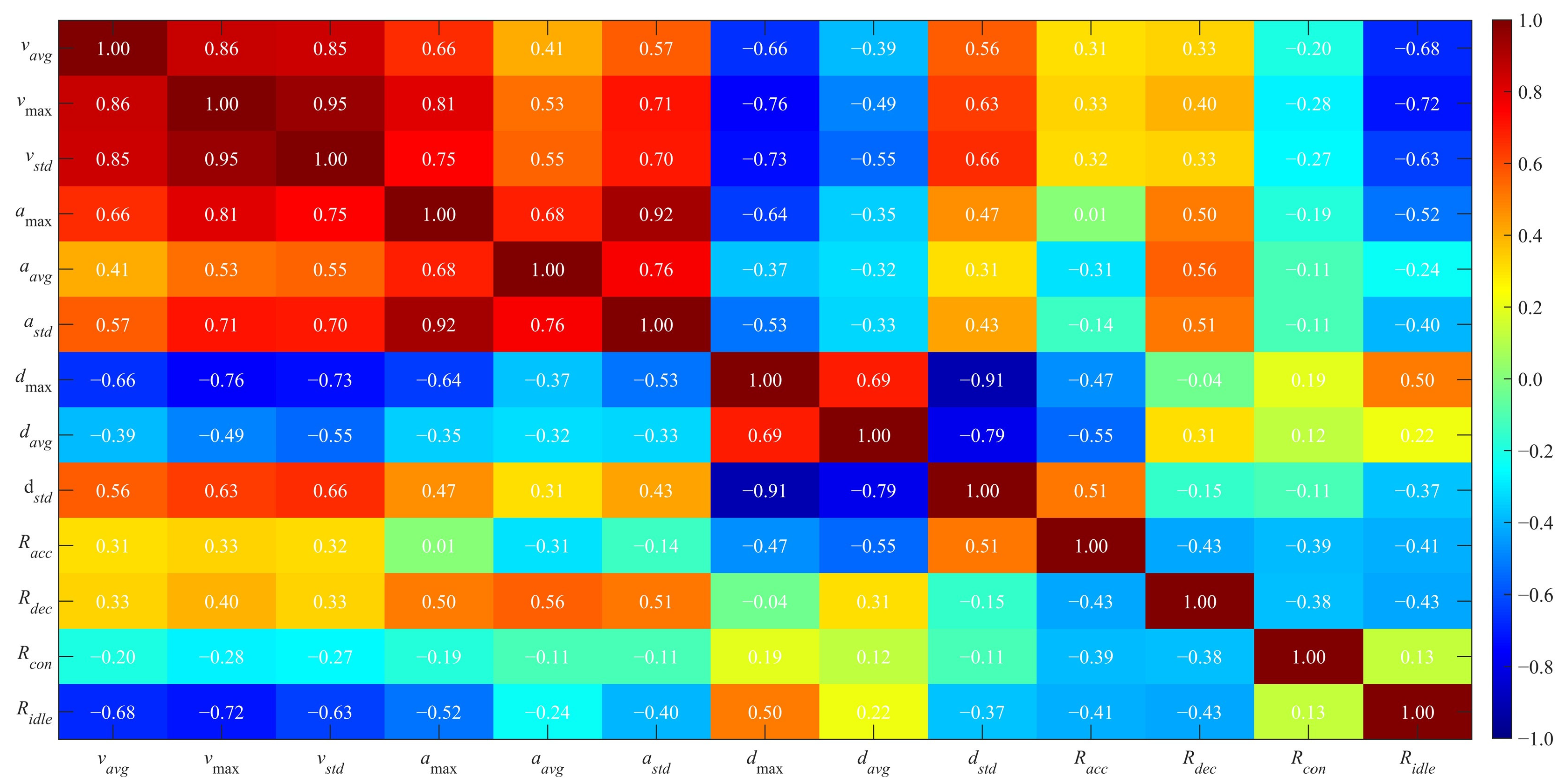
A correlation analysis was performed on the 13-dimensional features to examine their interrelationships and identify information overlap. Figure 8 displays a heatmap of Pearson correlation coefficients calculated using Formula (16). Significant correlations exist between multiple feature pairs, such as $v_{avg}$ with $v_{\mathrm{m}\mathrm{a}\mathrm{x}}$ and $v_{std}$, yielding correlation coefficients of 0.86 and 0.85, respectively. This information overlap indicates the necessity for dimensionality reduction.

3.2.2. PCA Dimensionality Reduction Results

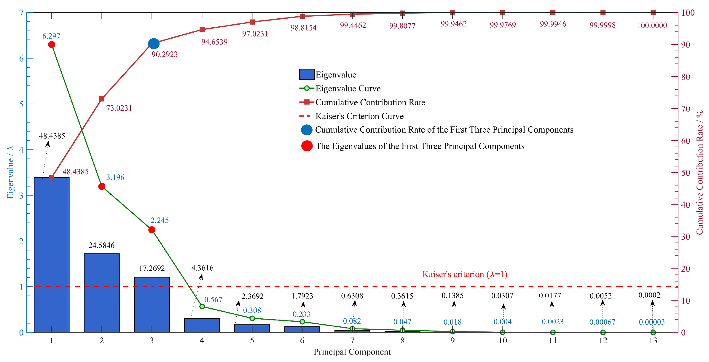
This study examined the trend of eigenvalues by plotting a scree plot (Figure 9) to determine the optimal number of principal components—components before the “elbow” typically contain the primary information, while those after often represent noise. In addition to the eigenvalue trend, the contribution rate and cumulative contribution rate of each principal component were comprehensively considered. As shown in Figure 9, according to the Kaiser criterion (retaining components with eigenvalues greater than 1), the first three principal components all have eigenvalues exceeding 1. Their cumulative contribution rate reaches $90.2923\%\approx 90.29\%$, meeting the standard in practical applications where the cumulative contribution rate is usually required to be between 85% and 95%. This effectively balances the trade-off between information retention and dimensionality reduction. Therefore, this study selected the first three principal components, reducing the original 13-dimensional features to 3 dimensions. This significantly lowers the time complexity for subsequent clustering algorithms while effectively filtering random noise from the data. By constructing a dimensionality reduction transformation matrix using the first three principal components, the original sailing condition data was projected onto the subspace spanned by these components, resulting in a new feature matrix ${\mathit{Y}}_{N\times 3}$. The principal component loading matrix is presented in

Table 4. Principal Component Loading Matrix.

Primitive Features	PC1	PC2	PC3
$v_{avg}$	0.912	−0.128	0.065
$v_{\mathrm{m}\mathrm{a}\mathrm{x}}$	0.886	−0.205	0.098
$v_{std}$	0.793	0.302	−0.114
$a_{\mathrm{m}\mathrm{a}\mathrm{x}}$	0.145	0.901	0.213
$d_{\mathrm{m}\mathrm{a}\mathrm{x}}$	0.208	0.872	−0.156
$a_{avg}$	0.327	0.786	0.417
$d_{avg}$	0.286	0.754	−0.382
$a_{std}$	−0.104	0.668	0.605
$d_{std}$	0.098	0.592	−0.587
$R_{con}$	0.874	0.235	0.108
$R_{acc}$	−0.217	0.903	0.187
$R_{dec}$	0.185	0.815	−0.224
$R_{idle}$	0.765	−0.312	0.411

. It can be observed that the first three principal components exhibit varying degrees of correlation with the original 13 features while maintaining low correlation with each other, further demonstrating their sufficiency in representing the overall information of the original features. Furthermore, by analyzing the loading coefficients of each principal component on the original features, their physical meanings can be interpreted: Principal Component 1 has high loadings on features such as average speed, maximum speed, and constant speed time ratio, primarily reflecting the overall sailing intensity and steady-state operational level. Principal Component 2 is closely related to acceleration-related parameters ($a_{\mathrm{m}\mathrm{a}\mathrm{x}}$, $R_{acc}$) and deceleration magnitude ($d_{\mathrm{m}\mathrm{a}\mathrm{x}}$), representing dynamic variation characteristics and maneuver aggressiveness. Principal Component 3 is mainly associated with acceleration and deceleration fluctuation characteristics ($a_{std}$, $d_{std}$), characterizing the smoothness or jerkiness of motion transitions. This interpretation aligns with the operational physics of harbor tugs, where intensity, dynamics, and smoothness are key dimensions of variability.

3.3. Kinematic Segment Clustering Results

3.3.1. Clustering Performance Evaluation Framework

The choice of the number of clusters, $K$, significantly impacts the results. If $K$ is too small, subtle operational differences cannot be distinguished; if $K$ is too large, the same operational mode may be overly fragmented, losing its physical meaning. This study employs a combined approach using the elbow method and the silhouette coefficient to comprehensively determine the optimal $K$ value.

(1)

Silhouette Coefficient Method

The silhouette coefficient, which combines intra-cluster cohesion and inter-cluster separation, is an important metric for evaluating clustering performance.

For each sample $i$, its silhouette coefficient s(i) is defined as:

$$s(i)={\displaystyle \frac{b(i)-a(i)}{\max \{a(i),b(i)\}}},$$

(47)

where $a(i)$ is the average distance from sample $i$ to other samples in the same cluster (cohesion), and $b(i)$ is the average distance from sample $i$ to samples in the nearest neighboring cluster (separation). The value of $s(i)$ ranges from −1 to 1, with values closer to 1 indicating better clustering.

The overall silhouette coefficient is the average of the silhouette coefficients for all samples:

$$S={\displaystyle \frac{1}{n}}{\sum }_{i=1}^{n}s(i),$$

(48)

The interpretation of the silhouette coefficient is as follows:

$s(i)\approx 1$: Sample $i$ is well-clustered.

$s(i)\approx 0$: Sample $i$ lies on the boundary between two clusters.

$s(i)\approx -1$: Sample $i$ is likely assigned to the wrong cluster.

The optimal $K$ value within the range $k\in [2, 10]$ is selected by identifying the $K$ that maximizes the overall silhouette coefficient.

(2)

Elbow Method

The within-cluster SSE is calculated for different values of $K$. As $K$ increases, SSE gradually decreases. When $K$ increases beyond a certain point, the rate of decrease in SSE slows down noticeably, forming an “elbow.” This point is considered the optimal $K$ value.

Calinski–Harabasz Index (CH)

The CH index evaluates clustering performance by calculating the ratio between the between-cluster dispersion and the within-cluster dispersion:

$$\mathrm{CH}={\displaystyle \frac{\mathrm{tr}(B_k)/(k-1)}{\mathrm{tr}(W_k)/(n-k)}},$$

(49)

where

$B_k$ is the between-cluster dispersion matrix: $B_k={\sum }_{i=1}^k{n}_i({\mu }_i-\mu )({\mu }_i-\mu {)}^T$,

$W_k$ is the within-cluster dispersion matrix: $W_k={\sum }_{i=1}^k{\sum }_{x\in C_i}(x-{\mu }_i)(x-{\mu }_i{)}^T$,

$\mu$ is the overall mean vector;

$n_i$ is the number of samples in the $i\text{-}\mathrm{th}$ cluster;

A higher CH value indicates better clustering performance.

Davies–Bouldin Index (DB)

The DB index measures the balance between intra-cluster compactness and inter-cluster separation:

$$DB={\displaystyle \frac{1}{k}}{\sum }_{i=1}^k{max}_{j\ne i}\left({\displaystyle \frac{{\sigma }_i+{\sigma }_j}{d(c_i,c_j)}}\right),$$

(50)

where:

${\sigma }_i={\displaystyle \frac{1}{|C_i|}}{\sum }_{x\in C_i}\Vert x-c_i\Vert$ is the average intra-cluster distance for cluster $I$;

$d(c_i,c_j)=\Vert c_i-c_j\Vert$ is the distance between the centroids of clusters $i$ and $j$.

A lower DB value indicates better clustering performance.

Within-Cluster SSE

SSE is calculated as:

$$SSE={\sum }_{i=1}^N(y_i-{\widehat{y}}_i{)}^2,$$

(51)

where $y_i$ is the actual value and ${\widehat{y}}_i$ is the model’s predicted value. SSE measures the total error between the model’s predictions and the actual values. It is often used directly as a loss function or fitness function in optimization.

3.3.2. WOA-K-Means++ Clustering Results

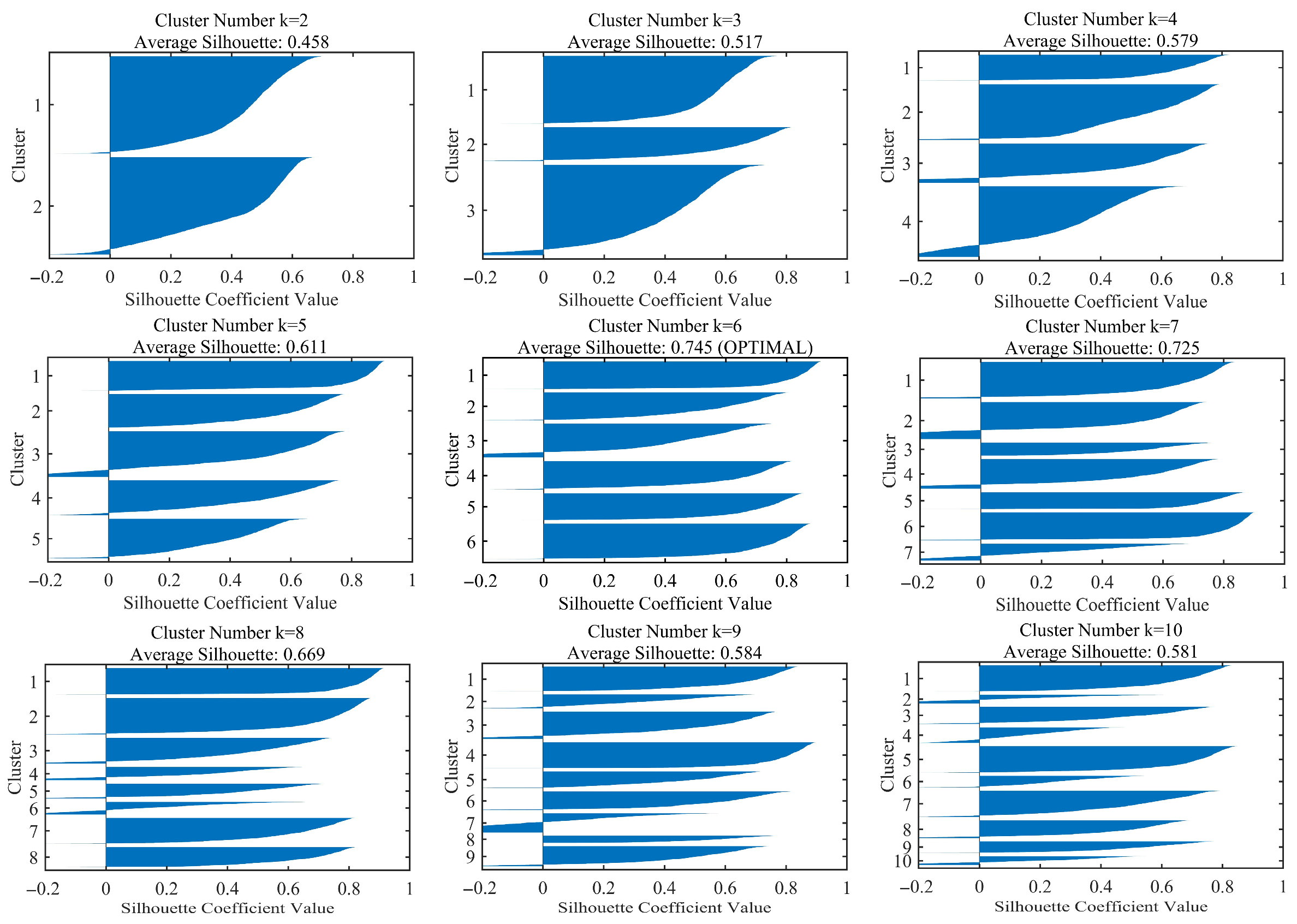
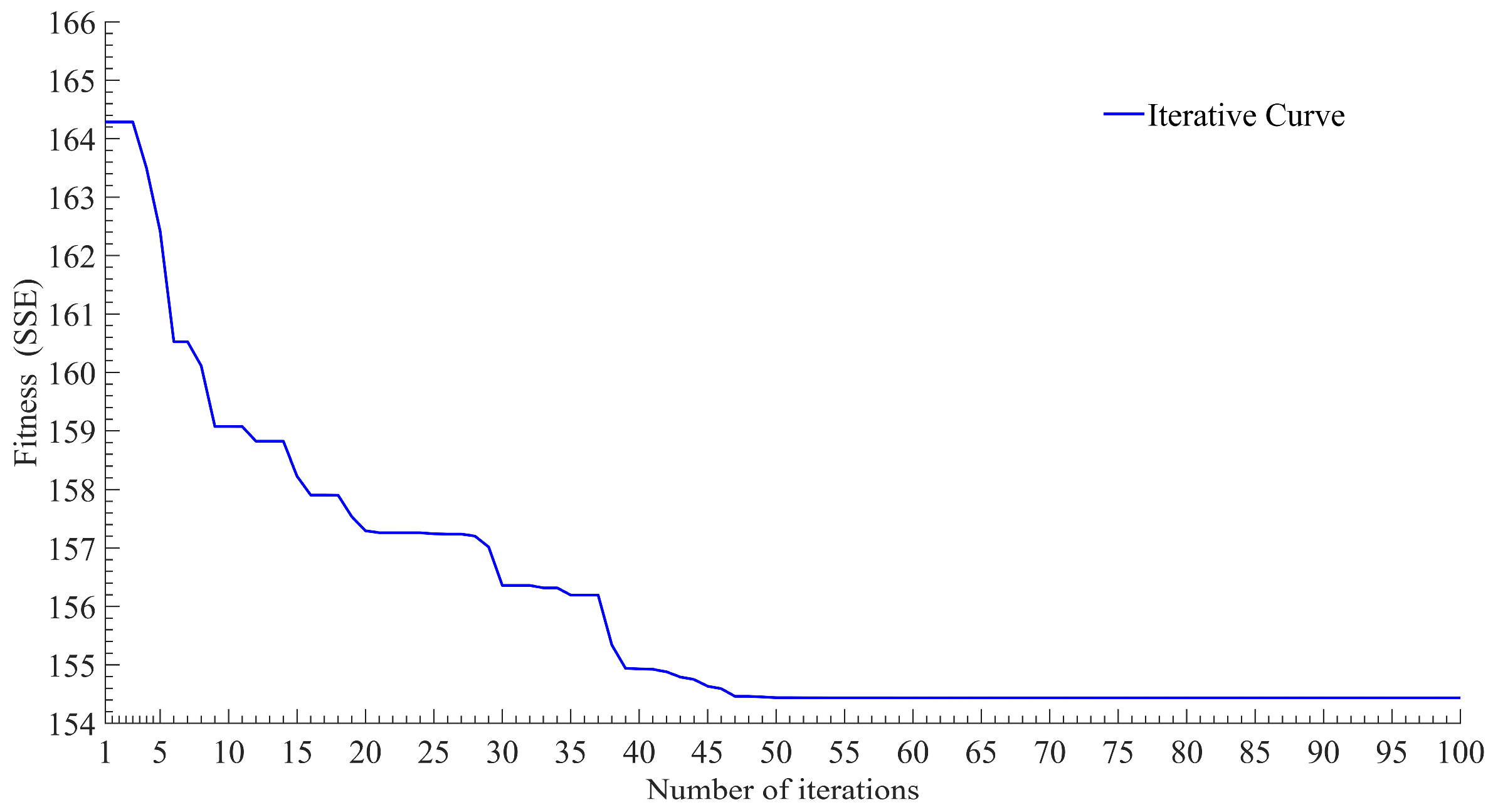
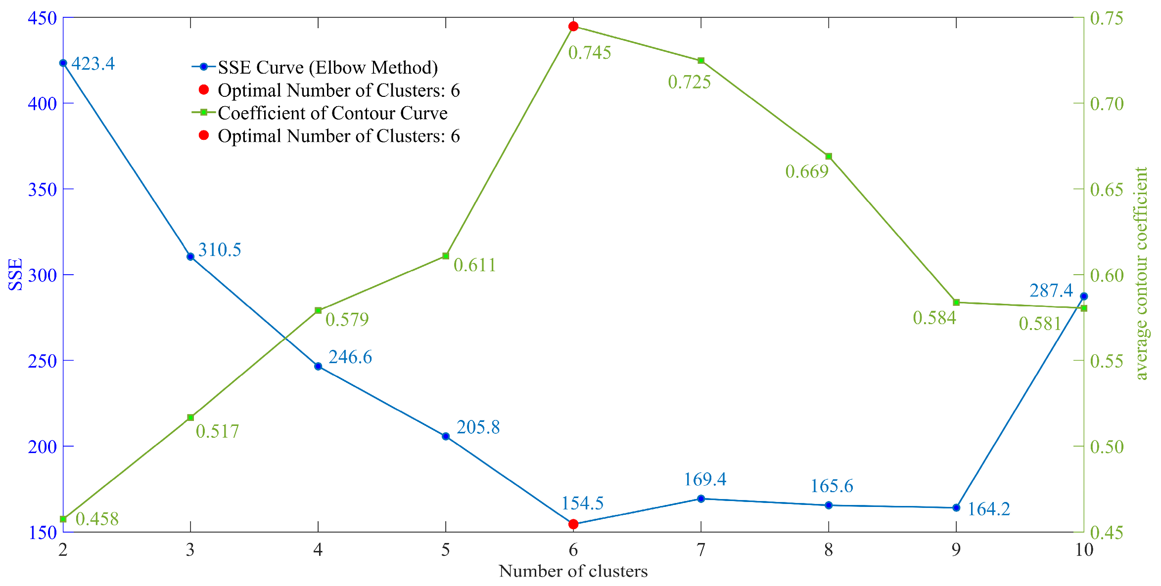
To determine the optimal number of clusters, this study employed a combined approach using the elbow method and the silhouette coefficient, supported by cross-validation with multiple clustering evaluation metrics. Figure 10, presented in the form of silhouette coefficient plots, compares the distribution of silhouette coefficients for clustering results with the number of clusters $K$ ranging from 2 to 10. When $K=6$, the silhouette coefficient values for all six clusters exceed 0.7, and the average silhouette coefficient reaches 0.745—the highest among all tested cluster counts. This indicates that the clustering structure is statistically most clear and reasonable at this point. Figure 11 shows the fitness (i.e., SSE) convergence curve of the WOA-K-means++ clustering algorithm when the number of clusters is set to 6. The horizontal axis represents the iteration count, and the vertical axis represents the fitness value (SSE). The optimization objective of the algorithm is to minimize SSE by iteratively adjusting the cluster centers. Therefore, the decrease in the SSE value directly reflects a reduction in model error, signifying enhanced compactness of samples within clusters. This convergence curve exhibits typical characteristics of an optimization process: in the initial iterations, leveraging the global search mechanism of the WOA, the SSE value rapidly declines, indicating the algorithm is extensively exploring the solution space. As iterations progress, the decreasing trend of SSE gradually slows, eventually stabilizing after approximately 47 iterations. The SSE value decreases from an initial 164.3 to a final 154.5, demonstrating that the algorithm has converged to a favorable clustering solution. This result validates the effectiveness of the WOA mechanism—by simulating the bubble-net hunting behavior of humpback whales, the algorithm effectively avoids local optima that traditional K-means++ might encounter, thereby providing a reliable guarantee for obtaining high-quality and stable initial cluster centers.

Table 5. Evaluation Metrics for the WOA-K-means++ Clustering Algorithm Across Different Numbers of Clusters.

Number of Clusters K	SEE	Mean Contour Coefficient Values	CH Index	DB Index
2	423.4	0.458	211.51	1.142
3	310.5	0.517	233.56	1.013
4	246.6	0.579	252.88	0.879
5	205.8	0.611	285.76	0.793
6	154.5	0.745	312.56	0.698
7	169.4	0.725	293.24	0.773
8	165.6	0.669	272.37	0.850
9	164.2	0.584	251.00	0.927
10	287.4	0.581	229.14	1.007

compares the within-cluster SSE, average silhouette coefficient, CH index, and DB index for different numbers of clusters. The results show that when $K=6$, the SSE is minimized (154.5), the average silhouette coefficient is maximized (0.745), the CH index is largest (312.56), and the DB index is smallest (0.698). All metrics consistently indicate that $K=6$ is the optimal number of clusters. Figure 12 further illustrates the analysis results of the elbow method and the silhouette coefficient method using a dual-axis plot. The left vertical axis (blue curve) represents SSE, the right vertical axis (green curve) represents the average silhouette coefficient, and the horizontal axis is the number of clusters $K$. As $K$ increases, the SSE curve shows a trend of rapid initial decline followed by a gradual leveling off, with a distinct elbow point appearing at $K=6$. Simultaneously, the silhouette coefficient curve peaks at $K=6$ (0.745) before gradually decreasing. The coincidence of the SSE elbow point and the silhouette coefficient peak at $K=6$ provides strong, complementary evidence from the perspectives of “model goodness-of-fit” and “intra-cluster compactness/inter-cluster separation,” jointly supporting the division of kinematic segments into 6 classes. In summary, the tabular data and graphical analysis results are highly consistent, confirming $K=6$ as the optimal number of clusters. This result not only establishes a reliable foundation for all subsequent analyses based on this clustering but also indicates that the complex operational process of the harbor tug can be reasonably characterized by six typical condition modes.

To quantitatively evaluate the performance advantages of the proposed WOA-K-means++ clustering algorithm, it was compared with the classic K-means and K-means++ algorithms on the same dataset. All three algorithms were set with a cluster number $K=6$ and run independently for 100 iterations to assess their average performance and stability. The evaluation covered nine dimensions: intra-cluster compactness (measured by average intra-cluster distance, lower is better), inter-cluster separation (measured by average silhouette coefficient, higher is better), convergence stability (measured by the standard deviation of results from multiple runs, lower is better), clustering stability (measured by the average pairwise Jaccard similarity coefficient across 100 runs, higher is better), CH index, DB index, SSE, number of iterations to convergence, and average runtime. As shown in

Table 6. Performance Comparison of Different Clustering Algorithms with the Same Number of Clusters.

Metric	K-Means	K-Means++	WOA-K-Means++
Average Intra-Cluster Distance	3.56	3.12	2.87
Average Silhouette Coefficient	0.635	0.692	0.745
Convergence Stability (Std. Dev.)	0.342	0.215	0.089
Clustering Stability	0.529	0.731	0.904
CH Index	275.43	289.67	312.56
DB Index	0.812	0.756	0.698
SEE	254.32	189.67	154.5
Iterations to Convergence	28	32	47
Average Runtime (second)	4.32	5.16	7.85

, WOA-K-means++ outperforms both K-means and K-means++ across the seven key metrics of intra-cluster compactness, inter-cluster separation, convergence stability, clustering stability, CH index, DB index, and SSE. Although there was an increase in the number of convergence iterations and average runtime, the increment is within an acceptable range and does not detract from the algorithm’s overall superior clustering performance. The reasons for this are analyzed as follows: While the K-means algorithm converges quickly, it is prone to getting stuck in local optima, and its results are sensitive to initial values. K-means++ improves convergence stability and the objective function value through better initialization, with convergence speed comparable to K-means. In contrast, WOA-K-means++, leveraging its stronger global search capability, converges to a better solution overall, even if convergence is slightly slower in the initial phase. The quantitative results in Table 6 fully demonstrate that the proposed WOA-K-means++ algorithm effectively reduces sensitivity to initial values and significantly enhances clustering quality.

To clarify the physical meaning of the six clusters (C1–C6), their cluster centers and data distributions were visualized, and the statistical characteristics of each cluster were analyzed in detail. Figure 13 and Figure 14 show the two-dimensional (PC1 vs. PC2) and three-dimensional (PC1, PC2, and PC3) scatter plots, respectively, generated based on the first three principal components from PCA dimensionality reduction and the WOA-K-means++ clustering results. Figure 13 displays the distribution of sample points in the plane formed by the first two principal components, with different clusters distinguished by color. Figure 14 further presents the clustered structure of data points in three-dimensional space. The figures show that sample points within the same cluster are densely grouped, forming clear “clumps,” while distinct gaps separate the different clusters. Although the low-dimensional projection loses some high-dimensional information, the images still effectively reflect the cluster structure in the original feature space. This visually verifies that after processing by the WOA-K-means++ algorithm, the six operational conditions exhibit the characteristics of intra-cluster compactness and inter-cluster separation in the feature space, once again proving the effectiveness of the clustering results from a geometric perspective.

Table 7. Statistical Means of Feature Parameters for the Six Operational Condition Classes.

Feature Parameters	C1	C2	C3	C4	C5	C6
$v_{avg}$/kn	0.8	3.2	5.6	7.9	10.3	12.5
$v_{\mathrm{m}\mathrm{a}\mathrm{x}}$/kn	2.5	5.8	8.9	11.6	13.8	15.0
$v_{std}$/kn	0.6	1.2	1.8	2.3	2.7	3.1
$a_{\mathrm{m}\mathrm{a}\mathrm{x}}$/m∙s−2	0.12	0.25	0.38	0.42	0.45	0.48
$d_{\mathrm{m}\mathrm{a}\mathrm{x}}$/m∙s−2	0.15	0.28	0.35	0.39	0.42	0.46
$a_{avg}$/m∙s−2	0.05	0.12	0.18	0.22	0.25	0.28
$d_{avg}$/m∙s−2	0.06	0.14	0.20	0.24	0.27	0.30
$a_{std}$/m∙s−2	0.03	0.08	0.12	0.15	0.18	0.21
$d_{std}$/m∙s−2	0.04	0.09	0.13	0.16	0.19	0.22
$R_{con}$/%	15.2	28.6	35.8	42.3	46.5	51.2
$R_{acc}$/%	20.3	25.8	28.9	30.5	31.2	32.6
$R_{dec}$/%	22.7	24.3	26.8	28.9	29.5	30.1
$R_{idle}$/%	41.8	21.3	8.5	3.3	1.8	0.1
Percentage/%	18.6	25.3	22.8	16.5	12.1	4.7

lists the representative features, i.e., the cluster centers, corresponding to each condition category (C1–C6). C1 is the idle condition, with the lowest average speed (0.8 knots) and a small proportion of acceleration phases, primarily corresponding to fine-tuning and positioning operations within the harbor. C2 and C3 are the low-speed condition (average speed 3.2 knots) and medium-speed condition (average speed 5.6 knots), respectively. Together, they account for 48.1% of the data, representing the most frequently occurring operational states for the harbor tug, which aligns with the practical operational characteristic of limited harbor space where high-speed operation is typically unnecessary. C4 and C5 belong to the medium-high-speed condition (average speed 7.9 knots) and high-speed condition (average speed 10.3 knots), mainly corresponding to transit and repositioning tasks within the port area. C6 is the very-high-speed condition (average speed 12.5 knots), with the lowest occurrence frequency (only 4.7%), typically activated only during emergency or special response missions. Overall, the operational patterns of the harbor tug are highly concentrated in the medium- and low-speed ranges. This is consistent with the operational demand for prioritizing maneuverability over speed in actual operations and confirms that the condition classification results align with the practical operational logic.

3.4. Construction Results of the Typical Sailing Condition Based on HMM

3.4.1. Construction Results of the Typical Sailing Condition

To construct a typical sailing condition that accurately reflects the temporal characteristics of harbor tug operations, it is necessary to combine the kinematic segments represented by each cluster (i.e., different conditions) according to their natural sequence in actual operations. First, the transition probabilities between different conditions were calculated. Based on the total duration of the typical condition and the proportion of time each condition occupies in the original sailing condition data (see Table 7), a time allocation was assigned to each condition category. Subsequently, kinematic segments within each cluster were sorted by their distance to the cluster center (from closest to farthest), prioritizing the selection of the most representative segments. Guided by the state transition probabilities shown in the matrix (Figure 15), the selected segments were concatenated sequentially to synthesize the typical condition profile. This process continued until the time allocations for all condition categories and the total duration requirement were met. Finally, the last segment exceeding the required duration was truncated, and smoothing was applied to ensure a smooth transition, resulting in a typical sailing condition that combines statistical representativeness with realistic temporal dynamics.

Figure 15 presents the state transition probability matrix calculated using Equation (1). This $6\times 6$ matrix clearly reveals the patterns of speed state transitions during harbor tug operations, primarily reflected in three aspects:

(1)

The operational process exhibits a strong tendency for state persistence. The idle condition (C1) and the medium-speed condition (C3), as core operational states, have self-transition probabilities as high as 0.70 and 0.55, respectively, forming the foundation for operational stability.

(2)

State transitions follow a progressive principle, and the acceleration and deceleration processes are asymmetric. Transitions between adjacent states dominate (e.g., C1 → C2 probability is 0.25, C2 → C3 is 0.15). However, the deceleration path back from high-speed states is more direct (e.g., the probability of decelerating from very-high-speed C6 to medium-high-speed C4 is 0.25, higher than the probability of accelerating from high-speed C5 to C6, which is 0.15), reflecting the safety-first operational norm.

(3)

High-speed states are transient and highly controllable. The self-transition probability for the very-high-speed condition (C6) is extremely low (0.05). When exiting this state, it primarily transitions to medium-high-speed (C4) and high-speed (C5) states (combined probability 0.50). Concurrently, the system allows it to decelerate directly to medium- or low-speed states with significant total probability (0.45), including skipping intermediate states (e.g., C6 → C3 probability 0.20, C6 → C2 probability 0.15, C6 → C1 probability 0.10), ensuring a rapid return to safe operating ranges in emergencies.

Overall, the probability distribution structure of this transition matrix (e.g., the medium-high-speed condition C4 has a self-transition probability of 0.50, while cross-state transitions skipping more than two levels all have probabilities below 0.05) realistically replicates the operational characteristics of harbor tugs: predominance of medium- and low-speed operations, gradual speed changes, and efficient, rapid deceleration for emergencies.

The 3600 s typical sailing condition constructed based on the HMM is shown in Figure 16. This profile overall exhibits the typical operational characteristics of a harbor tug: frequent start-stops, significant speed fluctuations, and brief high-speed operation intervals. It realistically reflects the complexity and dynamics of its operational process. To intuitively assess the representativeness of the constructed condition, a randomly selected 3600 s ship speed sequence from the original sailing condition data (after kinematic segmentation) was used as a benchmark for real-world conditions. This benchmark was compared with the synthesized typical sailing condition (Figure 17). The comparison shows that the two curves have a high degree of similarity in overall trend and speed fluctuation range, but they do not exhibit point-by-point overlap, which would indicate overfitting. This suggests that the constructed typical sailing condition not only successfully replicates the statistical patterns and kinematic features of harbor tug operations but also, through the HMM’s modeling of state sequences, avoids mechanically copying the original data. Consequently, it possesses greater overall representativeness and better reflects the essential operational patterns of this ship type.

3.4.2. Multidimensional Validity Verification

To quantitatively verify the effectiveness of the constructed typical sailing condition, this study established a multi-criteria verification framework. The framework evaluates the representativeness of the condition from three dimensions—statistical characteristics, temporal properties, and distribution similarity—assessing it from macro, dynamic, and probabilistic perspectives, respectively. Statistical Characteristics Verification involves comparing the relative error rates between the typical sailing condition and the original sailing condition across 13 feature parameters:

$$E_i=\left|{\displaystyle \frac{F_{T,i}-F_{o,i}}{F_{o,i}}}\right|\times 100\%,$$

(52)

where $F_{T,i}$ and $F_{o,i}$ represent the value of the $i\text{-}th$ feature for the typical sailing condition and the original sailing condition, respectively.

As shown in

Table 8. Comparison of 13 Feature Values Between the Typical Sailing Condition and the Original Sailing Condition.

Feature Category	Feature Name	Typical Sailing Condition	Original Sailing Condition	Absolute Error
Speed Features	$v_{avg}$	5.25 kn	5.12 kn	0.13
	$v_{\mathrm{m}\mathrm{a}\mathrm{x}}$	14.16 kn	14.48 kn	−0.32
	$v_{std}$	0.373 kn	0.361 m/s	0.012
Acceleration Features	$a_{\mathrm{m}\mathrm{a}\mathrm{x}}$	0.27 m/s2	0.28 m/s2	−0.01
	$d_{\mathrm{m}\mathrm{a}\mathrm{x}}$	0.28 m/s2	0.27 m/s2	0.01
	$a_{avg}$	0.148 m/s2	0.153 m/s2	−0.005
	$d_{avg}$	0.162 m/s2	0.157 m/s2	0.005
	$a_{std}$	0.079 m/s2	0.081 m/s2	−0.002
	$d_{std}$	0.088 m/s2	0.090 m/s2	−0.002
Time Proportion Features	$R_{con}$	34.5%	35.2%	−0.7%
	$R_{acc}$	22.5%	21.8%	0.7%
	$R_{dec}$	20.2%	20.8%	−0.6%
	$R_{idle}$	21.7%	21.1%	0.6%

and Figure 18, the differences between the 13 feature values of the typical sailing condition and the original sailing condition are minor, with all relative errors below 4%. The average relative error is 2.88%. This indicates that the typical sailing condition closely approximates the overall level of the original sailing condition across all features, meeting the validity requirements with high fidelity, and demonstrates a high degree of consistency between the condition constructed by this method and the real condition.

Temporal properties verification focuses on the joint probability distribution of speed and acceleration, measured using a two-dimensional correlation coefficient. The authenticity of a ship’s sailing condition is reflected not only in its speed distribution but, more critically, in the rationality of its speed change process (acceleration). Therefore, this study calculated the joint probability distribution of speed-acceleration for the original and generated data, using the two-dimensional correlation coefficient ${\rho }_{va}$ as the evaluation metric. Acceleration was computed via the central difference method: $a_t=(v_{t+1}-v_{t-1})/(2∆t)$, where $∆t=1$ s. This coefficient comprehensively reflects the consistency of the linear dependence between speed and acceleration in the two datasets, calculated as:

$${\rho }_{va}={\displaystyle \frac{{\sum }_{m,n}(P_{orig}(m,n)-{\overline{P}}_{orig})(P_{gen}(m,n)-{\overline{P}}_{gen})}{\sqrt{{{\sum }_{m,n}(P_{orig}(m,n)-{\overline{P}}_{orig})}^2\cdot {\sum }_{m,n}(P_{gen}(m,n)-{\overline{P}}_{gen}{)}^2}}},$$

(53)

where $P_{orig}$ and $P_{gen}$ are the 2D joint probability matrices of speed-acceleration for the original sailing condition and the typical sailing condition, respectively, and $m,n$ are matrix indices. The calculated value is ${\rho }_{va}=0.942$. This high correlation coefficient indicates that the generated data not only reproduces the statistical patterns of “at what speed to sail” in the original data but also precisely replicates the dynamic temporal characteristics of “how the speed changes.” Key features from the original data, such as small acceleration fluctuations during low-speed cruising and large negative accelerations during high-speed emergency stops, are preserved in the generated data.

Figure 19 presents the joint speed-acceleration distributions of the original sailing condition (left) and the typical sailing condition (right) as heatmaps. Both exhibit a similar structure with high-probability cores in the “low speed, low acceleration” and “medium speed, medium acceleration” regions. The negative acceleration (deceleration) patterns in high-speed regions of the typical sailing condition also show high agreement with the original sailing condition, verifying the effectiveness of the HMM model in generating dynamic sequences that conform to physical laws.

Distribution similarity verification employs the KL divergence to compare the speed distribution differences. KL divergence is a classical metric for measuring the difference between two probability distributions. For discrete distributions, the KL divergence between the speed distribution P of the original sailing condition and the speed distribution $Q$ of the typical sailing condition is defined as:

$$D_{KL}(P\parallel Q)={\sum }_{i}P(i)log{\displaystyle \frac{P(i)}{Q(i)}},$$

(54)

where $P$ and $Q$ represent the speed distribution histograms of the typical sailing condition and the original sailing condition, respectively, and $i$ indexes the bins of the speed histogram. A smaller $D_{KL}$ value indicates greater similarity between the two distributions, with 0 signifying identical distributions. In this study, the original and typical sailing conditions were divided into 50 bins each to compute their empirical probability distributions, yielding a KL divergence of $D_{KL}=0.023$.

To provide a holistic, quantitative performance evaluation of the proposed “WOA-K-means++ & HMM” condition construction method, a comprehensive scoring model was developed. This model assesses performance from three core dimensions—“Statistical Feature Fidelity,” “Temporal Property Fidelity,” and “Distribution Similarity”—with weights assigned as 0.4, 0.3, and 0.3, respectively, based on their importance in engineering applications. The model integrates multiple verification metrics into a single score for ease of overall quality assessment.

The scoring formula is:

$$S_{total}=w_1\cdot S_{stat}+w_2\cdot S_{dist}+w_3\cdot S_{time},$$

(55)

where $w_1$, $w_2$, $w_3$ are weighting coefficients, set to 0.4, 0.3, and 0.3, respectively. The score range is 0–100, with higher scores indicating closer resemblance between the typical and original sailing conditions.

(1) Statistical Feature Fidelity Score ($S_{stat}$, weight $w_1=0.4$):

This dimension’s score is based on the average relative error rate (2.88%) of the 13 features from

Table 9. Comprehensive Performance Scoring Table for Condition Construction Results.

Evaluation Dimension	Core Metric	Metric Value	Dimension Score (S)	Weight (w)	Weighted Score
Statistical Feature Fidelity	Avg. Relative Error of Multiple Statistics	2.88%	97.12	0.4	38.85
Distribution Similarity	KL Divergence $D_{KL}$	0.023	95.4	0.3	28.62
Temporal Property	Joint Dist. Corr. Coef. ${\rho }_{va}$	0.942	94.2	0.3	28.26
Total Comprehensive Score	$S_{total}=\sum (w_i·S_i)$	-	-	-	95.73

. Converting this to a percentage score: $S_{stat}=100\times (1-0.0288)=97.12$.

(2) Distribution Similarity Score ($S_{dist}$, weight $w_2=0.3$):

This dimension uses the KL divergence ($D_{KL}=0.023$) as the core metric. The score mapping is defined as: if $D_{KL}<0.03$, then $S_{dist}=100-200\times D_{KL}$. Calculation yields: $S_{dist}=100-200\times 0.023=95.4$.

(3) Temporal Property Score ($S_{time}$, weight $w_3=0.3$):

This dimension uses the joint speed-acceleration distribution correlation coefficient (${\rho }_{va}=0.942$) as the core metric. The score is defined as: $S_{time}=100\times {\rho }_{va}=94.2$.

The comprehensive score $S_{total}$ is calculated as follows:

$$S_{total}=w_1·S_{tate}+w_2·S_{dist}+w_3·S_{time}=0.4\times 97.12+0.3\times 95.4+0.3\times 94.2=95.73.$$

Statistical Significance Testing: To rigorously assess the improvement of the proposed WOA-K-means++ & HMM method over baseline clustering (K-means, K-means++) followed by simple random segment concatenation, a paired t-test was conducted on the comprehensive scores ($S_{total}$) derived from 50 bootstrap resamples of the dataset. The proposed method achieved a mean score of 95.73 with a standard deviation of 1.2, significantly higher than K-means ($85.4\pm 3.1$, $p<0.001$) and K-means++ ($90.1\pm 2.3$, $p<0.01$). This confirms that the improvement is statistically significant. To further validate the superiority of the proposed ‘WOA-K-means++ & HMM’ framework in profile synthesis, it was compared against a commonly used baseline method: using the same WOA-K-means++ clustering results but without employing HMM for state sequence modeling. Instead, kinematic segments were selected and concatenated completely randomly according to the time proportion of each cluster (hereafter referred to as the ‘random splicing method’). Evaluated using the same comprehensive scoring model (Equation (55)), the random splicing method achieved a total score of only 82.1. Its main loss was in the ‘Temporal Property Fidelity’ dimension ($S_{time}=78.5$), with a joint speed-acceleration distribution correlation coefficient ${\rho }_{va}$ of only 0.785, significantly lower than our method (0.942). This demonstrates that while the random splicing method can approximate macro statistical features, it fails to effectively preserve the temporal dynamic logic of state transitions present in the original data. The HMM modeling step introduced in this study is crucial for generating a high-fidelity, temporally rational typical profile.

Engineering Significance of Validation Metrics: The low average feature error (2.88%) ensures that the synthesized profile matches the overall energy demand and speed distribution of real operations, crucial for energy consumption simulations. The high joint distribution correlation (0.942) indicates that the dynamic acceleration/deceleration patterns are realistically preserved, which is vital for assessing engine transient loads and emissions. The low KL divergence (0.023) confirms that the speed probability distribution is accurately replicated, important for probabilistic risk assessments. The high comprehensive score (95.73) provides a single, interpretable metric for overall fidelity, useful for engineers comparing different condition construction methods.

As shown in Table 9, the typical sailing condition constructed in this study achieves a high comprehensive score of 95.73 out of 100. This indicates that the constructed typical sailing condition profile maintains high consistency with the original data across three key aspects: statistical characteristics, probability distribution, and temporal dynamics. This quantification fully validates the effectiveness and superiority of the integrated “WOA-K-means++ clustering” and “HMM modeling” method. The generated condition profile can highly credibly represent the various modes and their dynamic evolution in real harbor tug operations, providing a solid and reliable data foundation for subsequent energy efficiency analysis, simulation testing, and system design.

4. Discussion

4.1. Summary of Key Findings

The principal outcomes and implications of this study are succinctly summarized as follows:

Enhanced Clustering Performance: The proposed WOA-K-means++ algorithm effectively addresses the sensitivity to initialization and propensity for local optima common in traditional clustering methods. It reliably identified six distinct sailing condition clusters with clear physical interpretations, outperforming standard K-means and K-means++ across multiple evaluation metrics (see Table 9).

Effective Temporal Modeling: The HMM trained on these clusters successfully captured the intrinsic state transition logic of harbor tug operations. The derived probability matrix reflects characteristic patterns such as the prevalence of low/medium-speed states, sequential acceleration/deceleration, and direct transition paths for rapid deceleration (see Figure 15).

High-Fidelity Profile Synthesis: The synthesized 3600 s typical sailing condition demonstrates high consistency with the original operational data across statistical, temporal, and distributional dimensions. This is quantitatively validated by a low average feature error (2.88%), a high joint speed-acceleration distribution correlation (0.942), a low KL divergence (0.023), and a resulting comprehensive evaluation score of 95.73.

Methodological Transferability: While developed for a specific harbor tug, the integrated framework of data processing, feature engineering, optimized clustering, and HMM-based sequence synthesis is conceptually adaptable to constructing operational profiles for other ship types or mobile machinery with similar stop-go dynamic characteristics.

4.2. Research Prospects

The high-fidelity typical sailing condition for harbor tugs constructed in this study holds clear application value for operational management, energy strategy optimization, and port emission policy formulation. At the operational management level, this typical profile can serve as a standardized test cycle to evaluate and compare the energy consumption and emission performance under different tug designs (e.g., hybrid power systems, new propellers) or different operational strategies (e.g., route planning, power allocation). This provides quantitative evidence for fleet managers in technology selection and operational optimization. At the energy strategy optimization level, the typical profile reveals the operational pattern where tugs primarily operate at low/medium speeds and the transient, controllable nature of high-power states. This can guide the capacity configuration and energy management strategy design for hybrid power systems (e.g., batteries, supercapacitors), such as prioritizing the use of energy storage systems during frequent start-stop phases to improve overall energy efficiency and reduce main engine emissions. At the port emission policy formulation level, emission simulations based on the typical profile can more accurately estimate the actual emission contribution of mobile sources like harbor tugs, compensating for the shortcomings of assessments based on static indices (e.g., EEXI). Regulatory bodies can utilize such typical profiles as tools to develop local port ship emission inventories or to evaluate the emission reduction effects of green port measures (e.g., shore power, switching to low-carbon fuels), thereby formulating more scientific and targeted emission reduction incentives or regulations.

While the proposed WOA-K-means++ & HMM framework demonstrates high effectiveness in constructing a typical sailing condition for harbor tugs, several limitations and practical considerations warrant discussion.

Data Scope and Generalizability: The study relies on data from a single port and one tug type. Although the methodology is generic, the specific condition clusters and transition probabilities are data-driven and may vary for tugs operating in different ports, under different weather conditions, or with different propulsion systems. Future work should validate the approach with multi-port, multi-ship datasets.

Model Assumptions: The HMM assumes a first-order Markov property and discrete hidden states. While appropriate for capturing macro-level operational logic, this may oversimplify more complex, long-range dependencies or continuous state variations. Extensions such as higher-order Markov models or continuous HMMs could be explored.

Computational Cost: The WOA-K-means++ clustering, though accurate, incurs higher computational cost than standard K-means (Table 9). This is acceptable for offline profile construction but may be a constraint for real-time, onboard applications where computational resources are limited. For such scenarios, a pre-trained HMM could be deployed for rapid sequence generation.

Practical Deployment and Real-Time Applicability: For real-time energy management or emissions monitoring, the constructed typical condition serves as a benchmark rather than a real-time predictor. Integrating the method into a digital twin framework, where real-time AIS/data-logger data continuously updates the HMM parameters, could enable dynamic condition adaptation and more accurate real-time performance assessment.

Broader Implications: Beyond harbor tugs, the integrated clustering-HMM approach is applicable to other mobile machinery with stop-go, multi-modal operational patterns, such as terminal tractors, construction equipment, or urban delivery vehicles. The key is to adapt the feature set and segmentation rules to the specific context.

In summary, this study presents a robust, data-driven method for harbor tug condition construction, validated with high-fidelity metrics. Acknowledging its limitations opens avenues for future research in data expansion, model refinement, and real-time integration.

5. Conclusions

This study aimed to construct a high-fidelity typical sailing condition for harbor tugs to support their energy efficiency assessment and optimization. To address the complexity and temporal dynamics of tug operations, an integrated methodology combining PCA, an enhanced WOA-K-means++ clustering algorithm, and HMM-based sequence modeling was proposed and successfully applied to generate a representative 3600 s profile.

The main contributions and findings are threefold. First, the proposed WOA-K-means++ clustering algorithm effectively overcomes the sensitivity to initial centers and susceptibility to local optima inherent in traditional methods. It stably identified six distinct sailing condition types with clear physical meanings, outperforming standard K-means and K-means++ across multiple evaluation metrics. Second, the HMM constructed based on the optimal clustering results reasonably characterized the transition patterns between different condition states. The obtained state transition probability matrix reflects the core operational logic of harbor tugs, such as the prevalence of medium/low speeds and direct deceleration paths. Third, the constructed typical sailing condition profile demonstrated high consistency with the original data across statistical characteristics, temporal properties, and distribution similarity, achieving a comprehensive evaluation score of 95.73. This validates the effectiveness of the proposed framework in replicating real-world operational patterns.

This study has certain limitations that point to future research directions. The condition clusters and transition probabilities are data-driven and may require recalibration for tugs operating in different ports or with different specifications. Future work could validate and extend the method using multi-port, multi-ship datasets. The assumption of a first-order Markov process and discrete states could be explored further, for instance, by investigating higher-order or continuous HMMs. Additionally, integrating the constructed profile or the online learning HMM into a digital twin framework for real-time energy management and emission monitoring presents a promising practical application. Despite these limitations, the proposed methodological framework provides a reliable and adaptable tool for constructing operational profiles, not only for harbor tugs but potentially for other types of ships or mobile machinery with similar stop-go operational characteristics.

References

1. Chen, B.; Chen, F.; Ciais, P.; Zhang, H.; Lü, H.; Wang, T.; Chevallier, F.; Liu, Z.; Yuan, W.; Peters, W. Challenges to achieve carbon neutrality of China by 2060: Status and perspectives. Sci. Bull. 2022, 67, 2030–2035. [Google Scholar] [CrossRef] [Scilit]
2. Zhang, Y.; Liang, C.; Shi, J.; Lim, G.; Wu, Y. Optimal port microgrid scheduling incorporating onshore power supply and berth allocation under uncertainty. Appl. Energy 2022, 313, 118856. [Google Scholar] [CrossRef] [Scilit]
3. Murcia González, J.C. Analysis and measurement of SOx, CO2, PM and NOx emissions in port auxiliary vessels. Environ. Monit. Assess. 2021, 193, 374. [Google Scholar] [CrossRef] [Scilit] [PubMed]
4. Lebedevas, S.; Norkevičius, L.; Zhou, P. Investigation of effect on environmental performance of using LNG as fuel for engines in seaport tugboats. J. Mar. Sci. Eng. 2021, 9, 123. [Google Scholar] [CrossRef] [Scilit]
5. Hwang, S.; Lee, C.; Ryu, J.; Lim, J.; Chung, S.; Park, S. Optimal EMS Design for a 4-MW-Class Hydrogen Tugboat: A Comparative Analysis Using DP-Based Performance Evaluation. Energies 2024, 17, 3146. [Google Scholar] [CrossRef] [Scilit]
6. Cui, Y.; Zou, F.; Xu, H.; Chen, Z.; Gong, K. A novel optimization-based method to develop representative driving cycle in various driving conditions. Energy 2022, 247, 123455. [Google Scholar] [CrossRef] [Scilit]
7. Lee, H.; Lee, K. Comparative evaluation of the effect of vehicle parameters on fuel consumption under NEDC and WLTP. Energies 2020, 13, 4245. [Google Scholar] [CrossRef] [Scilit]
8. Lee, S.S. Analysis of the effects of EEDI and EEXI implementation on CO2 emissions reduction in ships. Ocean Eng. 2024, 295, 116877. [Google Scholar] [CrossRef] [Scilit]
9. Fan, A.; Fan, X.; Zhang, M.; Yang, L.; Xiong, Y.; Lang, X.; Sheng, C.; He, Y. Data-driven ship typical operational conditions: A benchmark tool for assessing ship emissions. J. Clean. Prod. 2024, 483, 144252. [Google Scholar] [CrossRef] [Scilit]
10. Devarapali, S.; Manske, A.; Khayamim, R.; Jacobs, E.; Li, B.; Elmi, Z.; Dulebenets, M. Electric tugboat deployment in maritime transportation: Detailed analysis of advantages and disadvantages. Marit. Bus. Rev. 2024, 9, 263–291. [Google Scholar] [CrossRef] [Scilit]
11. Greig, N.C.; Hines, E.M.; Cope, S.; Liu, X. Using satellite AIS to analyze vessel speeds off the coast of Washington State, US, as a Risk Analysis for Cetacean-Vessel Collisions. Front. Mar. Sci. 2020, 7, 109. [Google Scholar] [CrossRef] [Scilit]
12. Lin, B.; Wei, C.; Feng, F. A vehicle velocity prediction method with kinematic segment recognition. Appl. Sci. 2024, 14, 5030. [Google Scholar] [CrossRef] [Scilit]
13. Liu, X.; Ma, J.; Zhao, X.; Du, J.; Xiong, Y. Study on driving cycle synthesis method for city buses considering random passenger load. J. Adv. Transp. 2020, 2020, 3871703. [Google Scholar] [CrossRef] [Scilit]
14. Zähringer, M.; Kalt, S.; Lienkamp, M. Compressed driving cycles using Markov chains for vehicle powertrain design. World Electr. Veh. J. 2020, 11, 52. [Google Scholar] [CrossRef] [Scilit]
15. Ma, R.; He, X.; Zheng, Y.; Zhou, B.; Lu, S.; Wu, Y. Real-world driving cycles and energy consumption informed by large-sized vehicle trajectory data. J. Clean. Prod. 2019, 223, 564–574. [Google Scholar] [CrossRef] [Scilit]
16. Quirama, L.F.; Giraldo, M.; Huertas, J.I.; Tibaquirá, J.; Cordero Moreno, D. Main characteristic parameters to describe driving patterns and construct driving cycles. Transp. Res. Part D Transp. Environ. 2021, 97, 102959. [Google Scholar] [CrossRef] [Scilit]
17. Brady, J.; O’Mahony, M. Development of a driving cycle to evaluate the energy economy of electric vehicles in urban areas. Appl. Energy 2016, 177, 165–178. [Google Scholar] [CrossRef] [Scilit]
18. Bishop, J.D.K.; Axon, C.J. Using natural driving experiments and Markov chains to develop realistic driving cycles. Transp. Res. Part D Transp. Environ. 2024, 137, 104507. [Google Scholar] [CrossRef] [Scilit]
19. Almachi, J.C.; Saguay, J.; Anrango, E.; Cando, E.; Reina, S. Clustering-Based Urban Driving Cycle Generation: A Data-Driven Approach for Traffic Analysis and Sustainable Mobility Applications in Ecuador. Sustainability 2025, 17, 3353. [Google Scholar] [CrossRef] [Scilit]
20. Ay, M.; Özbakır, L.; Kulluk, S.; Gülmez, B.; Öztürk, G.; Özer, S. FC-Kmeans: Fixed-centered K-means algorithm. Expert Syst. Appl. 2023, 211, 118656. [Google Scholar] [CrossRef] [Scilit]
21. Li, H.; Wang, J. Collaborative annealing power k-means++ clustering. Knowl.-Based Syst. 2022, 255, 109593. [Google Scholar] [CrossRef] [Scilit]
22. Gao, Y.; Xu, Z.; Nie, F.; Zhang, Y.; Zhu, Q.; Shao, G. Joint Projected Fuzzy Neighborhood Preserving C-means Clustering with Local Adaptive Learning. Expert Syst. Appl. 2024, 255, 124617. [Google Scholar] [CrossRef] [Scilit]
23. Cheng, D.; Zhang, C.; Li, Y.; Xia, S.; Wang, G.; Huang, J.; Zhang, S.; Xie, J. GB-DBSCAN: A fast granular-ball based DBSCAN clustering algorithm. Inf. Sci. 2024, 674, 120731. [Google Scholar] [CrossRef] [Scilit]
24. Jing, Z.; Wang, T.; Zhang, S.; Wang, G. Development Method for the Driving Cycle of Electric Vehicles. Energies 2022, 15, 8715. [Google Scholar] [CrossRef] [Scilit]
25. Yan, W.; Li, M.; Zhong, Y.; Qu, C.; Li, G. A novel k-MPSO clustering algorithm for the construction of typical driving cycles. IEEE Access 2020, 8, 64028–64036. [Google Scholar] [CrossRef] [Scilit]
26. Zhao, L.; Li, K.; Zhao, W.; Ke, H.; Wang, Z. A sticky sampling and Markov state transition matrix based driving cycle construction method for EV. Energies 2022, 15, 1057. [Google Scholar] [CrossRef] [Scilit]
27. Dabčević, Z.; Škugor, B.; Topić, J.; Deur, J. Synthesis of driving cycles based on low-sampling-rate vehicle-tracking data and Markov chain methodology. Energies 2022, 15, 4108. [Google Scholar] [CrossRef] [Scilit]
28. Zhang, M.; Shi, S.; Cheng, W.; Shen, Y. Self-adaptive hyper-heuristic Markov chain evolution for generating vehicle multi-parameter driving cycles. IEEE Trans. Veh. Technol. 2020, 69, 6041–6052. [Google Scholar] [CrossRef] [Scilit]
29. Yuan, M.; Kan, X.; Chi, C.; Cao, L.; Shu, H.; Fan, Y. Study of driving cycle of city tour bus based on coupled GA-K-means and HMM algorithms: A case study in Beijing. IEEE Access 2021, 9, 20331–20345. [Google Scholar] [CrossRef] [Scilit]
30. Agushaka, J.O.; Ezugwu, A.E. Initialisation approaches for population-based metaheuristic algorithms: A comprehensive review. Appl. Sci. 2022, 12, 896. [Google Scholar] [CrossRef] [Scilit]
31. Rana, N.; Latiff, M.S.A.; Abdulhamid, S.M.; Chiroma, H. Whale optimization algorithm: A systematic review of contemporary applications, modifications and developments. Neural Comput. Appl. 2020, 32, 16245–16277. [Google Scholar] [CrossRef] [Scilit]
32. Chen, S.; Wang, F.; Wei, X.; Tan, Z.; Wang, H. Analysis of tugboat activities using AIS data for the Tianjin port. Transp. Res. Rec. 2020, 2674, 498–509. [Google Scholar] [CrossRef] [Scilit]
33. Wijaya, W.M.; Nakamura, Y. Port performance indicators construction based on the AIS-generated trajectory segmentation and classification. Int. J. Data Sci. Anal. 2025, 20, 2473–2492. [Google Scholar] [CrossRef] [Scilit]
34. Zhang, L.; Meng, Q.; Xiao, Z.; Fu, X. A novel ship trajectory reconstruction approach using AIS data. Ocean Eng. 2018, 159, 165–174. [Google Scholar] [CrossRef] [Scilit]
35. Wang, Y.; Li, K.; Zeng, X.; Gao, B.; Hong, J. Energy consumption characteristics based driving conditions construction and prediction for hybrid electric buses energy management. Energy 2022, 245, 123189. [Google Scholar] [CrossRef] [Scilit]
36. Zhang, J.; Wang, Z.; Liu, P.; Zhang, Z.; Li, X.; Qu, C. Driving cycles construction for electric vehicles considering road environment: A case study in Beijing. Appl. Energy 2019, 253, 113514. [Google Scholar] [CrossRef] [Scilit]
37. Yang, D.; Liu, T.; Zhang, X.; Zeng, X.; Song, D. Construction of high-precision driving cycle based on Metropolis-Hastings sampling and genetic algorithm. Transp. Res. Part D Transp. Environ. 2023, 118, 103715. [Google Scholar] [CrossRef] [Scilit]
38. He, H.; Guo, J.; Zhou, N.; Sun, C.; Peng, J. Freeway driving cycle construction based on real-time traffic information and global optimal energy management for plug-in hybrid electric vehicles. Energies 2017, 10, 1796. [Google Scholar] [CrossRef] [Scilit]
39. Guo, S.; Wu, K.; Zhang, G. Application of PCA-K-means++ combination model to construction of light vehicle driving conditions in intelligent traffic. J. Meas. Eng. 2020, 8, 107–121. [Google Scholar] [CrossRef] [Scilit]
40. Liu, L.; Zhang, R. Multistrategy improved whale optimization algorithm and its application. Comput. Intell. Neurosci. 2022, 2022, 3418269. [Google Scholar] [CrossRef] [Scilit]
41. Mirjalili, S.; Lewis, A. The whale optimization algorithm. Adv. Eng. Softw. 2016, 95, 51–67. [Google Scholar] [CrossRef] [Scilit]
42. Zhang, W.; Xu, Z.; Hong, Y.; Bi, Z. Onboard photovoltaic-energy storage system integration in high-speed trains: Economic-environmental optimization via IGWO-WOA algorithm. Appl. Energy 2025, 400, 126579. [Google Scholar] [CrossRef] [Scilit]
43. Ge, J.; Wang, T.; Hu, K.; Wang, J.; Wu, J.; Wang, J.; Wu, J. Optimization of power grid material warehousing and supply chain distribution path planning based on improved PSO algorithm. Sci. Rep. 2025, 15, 45132. [Google Scholar] [CrossRef] [Scilit] [PubMed]
44. Min, D.; Song, Z.; Chen, H.; Wang, T.; Zhang, T. Genetic algorithm optimized neural network based fuel cell hybrid electric vehicle energy management strategy under start-stop condition. Appl. Energy 2022, 306, 118036. [Google Scholar] [CrossRef] [Scilit]
45. Ma, J.; Pan, M.; Guan, W.; Zhang, Z.; Zhou, J.; Ye, N.; Qin, H.; Li, L.; Man, X. Economy Optimization by Multi-Strategy Improved Whale Optimization Algorithm Based on User Driving Cycle Construction for Hybrid Electric Vehicles. Machines 2025, 13, 158. [Google Scholar] [CrossRef] [Scilit]
Figure 1. A typical harbor tug at the Port of Dalian.
Jmse 14 00270 g001
Figure 2. Typical sailing trajectory of the harbor tug.
Jmse 14 00270 g002
Figure 3. Technical Approach.
Jmse 14 00270 g003
Figure 4. Ship Speed Data Processing Workflow.
Jmse 14 00270 g004
Figure 5. Typical Kinematic Segment.
Jmse 14 00270 g005
Figure 6. K-means++-Based Kinematic Segment Clustering Process.
Jmse 14 00270 g006
Figure 7. Workflow for Constructing the Typical Sailing Condition Based on HMM.
Jmse 14 00270 g007
Figure 8. Kinematic Fragment 13-Dimensional Feature Correlation Matrix Diagram.
Jmse 14 00270 g008
Figure 9. Eigenvalues and Contribution Rates of Principal Components.
Jmse 14 00270 g009
Figure 10. Comparison of Silhouette Coefficients for Different Numbers of Clusters.
Jmse 14 00270 g010
Figure 11. Fitness Convergence Curve of the WOA-K-means++ Clustering Algorithm.
Jmse 14 00270 g011
Figure 12. Determining the Optimal Number of Clusters Curve Using the Elbow Method and Contour Coefficient Method.
Jmse 14 00270 g012
Figure 13. Two-dimensional Clustering Projection Plot (First Two Principal Components).
Jmse 14 00270 g013
Figure 14. Three-dimensional Cluster Plot (First Three Principal Components).
Jmse 14 00270 g014
Figure 15. State Transition Probability Matrix Between Different Clusters.
Jmse 14 00270 g015
Figure 16. Vessel Speed Profile of the Typical Sailing Condition.
Jmse 14 00270 g016
Figure 17. Comparative Curves of the Typical Sailing Condition and the Original Sailing Condition.
Jmse 14 00270 g017
Figure 18. Comparison of Relative Error Rates for the 13 Features Between the Typical and Original Sailing Conditions.
Jmse 14 00270 g018
Figure 19. Comparison of Joint Speed-Acceleration Distributions.
Jmse 14 00270 g019