Analysis of Wave Height and Period in the Yangtze River Delta and Adjacent Waters Based on a 31-Year High-Resolution Wave Hindcast

Abstract

This study presents a 31-year (1993–2023) wave hindcast using a high-resolution two-domain nested numerical wave model implemented with Simulating Waves Nearshore (SWAN). The spatiotemporal variability and long-term trends of two wave parameters (significant wave height H_s and spectral peak period T_peak) are systematically analyzed for the Yangtze River Delta (YRD) and its adjacent waters. Validation against in situ buoy measurements confirms that the SWAN model effectively reproduces the regional wave conditions. Results indicate that mean wave conditions are primarily modulated by the Asian monsoon, whereas extreme wave events are predominantly influenced by typhoons. This leads to pronounced differences in spatial patterns and seasonal variability between mean and maximum H_s values. In addition, the regional interannual variations of H_s and T_peak exhibit different degrees of correlation with the Niño 3.4 index, the Pacific Decadal Oscillation (PDO) index and the Western Pacific Subtropical High Ridge Position (WPSH) Index. Overall, both H_s and T_peak exhibit positive trends over the study period, and both positive trends shift remarkably between seasons. The positive trends in mean wave conditions are mild during spring and summer but more pronounced in autumn and winter. Statistically significant increases in seasonal mean H_s are identified in parts of the East China Sea (0.35 cm a⁻¹ in autumn) and the southern Yellow Sea (0.27 cm a⁻¹ in winter). Notably, not all trends are positive: the 90th percentiles of both H_s and T_peak during summer exhibit widespread declining trends, although they are not statistically significant.

1. Introduction

Surface waves are a fundamental dynamic component of the ocean environment, playing an important role in momentum and energy exchange between oceans and the atmosphere [1]. Their interactions with winds, currents and shorelines shape ocean circulation, weather and climate [2,3]. Beyond their geophysical importance, waves also serve as a basis for maritime navigation and coastal engineering. The continuous action of waves on marine structures induces mechanical fatigue, a key factor that must be accounted for in their design and durability assessment [4]. Wave energy also offers a renewable resource to mitigate climate change [5].

However, increasing evidence shows that the statistical characteristics of waves are strongly modulated by climate change, primarily through alterations in local wind speed, sea level pressure and teleconnections [6,7]. Understanding these shifts in wave climate is crucial for developing effective adaptation strategies in a warming world. Historical data and future wave projections are commonly used to detect such changes. Given the high uncertainties in wave projections [8,9], it is of particular importance to construct historic wave climates to establish a robust reference dataset and correct bias in future wave climate projections [10,11].

Four types of historical data are used in retrieving the historical wave climate: in situ observations, satellite remote sensing data, open access wave reanalyses, and model wave hindcasts. In situ wave observations and satellite remote sensing data can offer long-term quantitative measurements of wave conditions [12,13], but both have limitations. In situ observations are always spatially sparse [8], while satellite data are subject to considerable uncertainties arising from different multimission calibration procedures [14]. As a result, wave hindcast and reanalysis datasets are often adopted as observational proxies. These products offer continuous, uninterrupted wave data with high spatial and temporal resolution [15,16]. These advantages result in their wide application in investigations of the historical wave climate at both global and regional scales [7,17]. Compared to open access reanalysis datasets, such as the widely-used ERA5, wave hindcasts based on numerical models, including WAVEWATCH III [18,19], Simulating Waves Nearshore (SWAN) [20,21], and WAM [22,23], can achieve higher spatial resolutions. Although they typically do not assimilate wave observations, this very feature allows them to overcome certain limitations of reanalysis products. The enhanced resolution supports more accurate wave assessments in coastal regions, making hindcasts particularly valuable for studying wave dynamics at local scales.

Various historic wave climate products have been constructed and analyzed across the globe and in different regions. Reguero et al. [24] developed a global ocean wave dataset based on WAWVEWATCH III model for global wave climate variability analysis since 1948. Smith et al. [25] proposed a global wave hindcast dataset with an Australian and Pacific Island focus. Given the abundance of global ocean wave reanalysis and hindcast products, Morim et al. [15] established a standardized framework to sample wave data across 14 products at different frequency resolutions (monthly, seasonally, and annually). Mirzaei et al. [26] employed a 31-year wave hindcast to analyze the wave climate in the southern South China Sea and found that wave heights tend to increase during May, July and September but decrease in December in the Sunda shelf region. Gemmrich et al. [27] analyzed wave heights from seven northeast Pacific wave records and found positive trends in southern locations but negative trends in northern buoys. Elshinnawy et al. [18] performed a 64-year wave hindcast in the Red Sea using a WAVEWATCH III model and found that long-term trends are mild under average and extreme conditions.

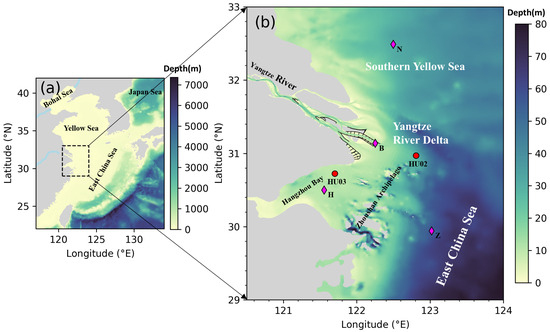
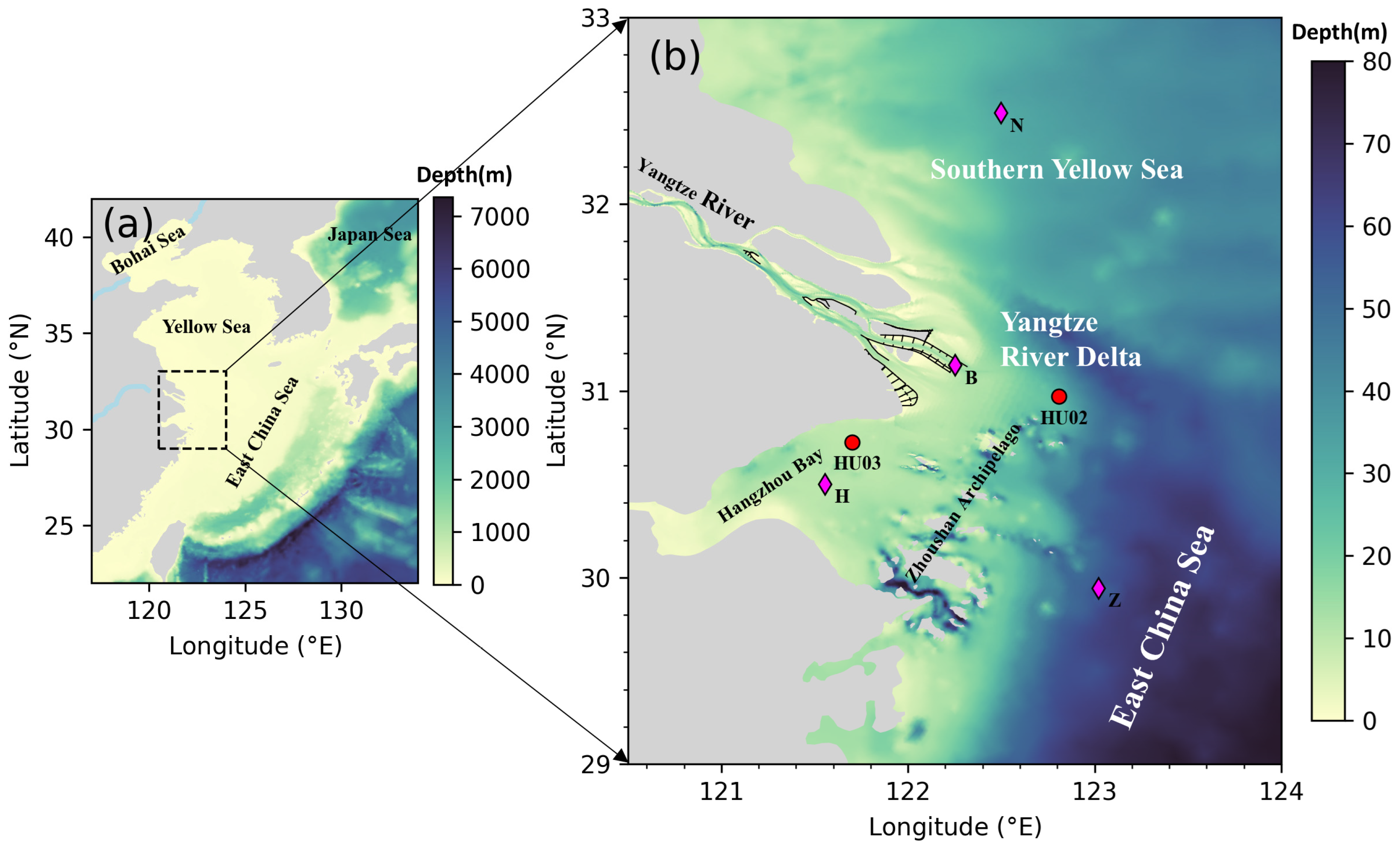
The Yangtze River Delta (YRD) and the adjacent waters, including the Zhoushan Archipelago and Hangzhou Bay, are among the busiest waters in China (Figure 1). This area is beside the East China Sea (ECS). Two international ports that number among the top ten globally, namely, the Shanghai international shipping center and Ningbo–Zhoushan port, are located at this region. It is one of China’s core regions, with high population density and strong economic vitality [28]. As a consequence, this area has been extensively constructed (Figure 1b) for the benefit of ship navigation, water supply, and land demand [29]. This region is strongly impacted by the Asian monsoon wind system, with a primary strong northerly or northeasterly wind in winter and a mild southerly or southeasterly wind in summer. Each summer and autumn, typhoons hit this area, leading to remarkable waves [30]. A high-resolution wave forecast system has been developed to serve this area [31].

Figure 1. (a) Topographic map of the Yangtze River Delta (YRD), the East China Sea and the adjacent open ocean, with the black dashed line indicating the key study area of this study. (b) Location and geographic setting of the YRD and adjacent waters. The red bullets denote location of the wave buoys. The magenta diamonds signify four representative stations for analysis. The black lines represent the main engineering constructions in the Yangtze River Estuary.

Many studies have investigated wave climate in this area, but most of them focused on the ECS or a larger domain. Zheng et al. [32] investigated long-term wave characteristics in the ECS using 30 years (1980–2009) of wave hindcast data by WAVEWATCH III and concluded that the southwest ECS tends to experience rough and very rough seas more frequently. Wang et al. [17] analyzed the wave climate in the ECS, adopting the ERA-40 and ERA datasets, and indicated that the wave height over the ECS increased by 0.5–1.0 cm a⁻¹, with El Niño–Southern Oscillation (ENSO) and Pacific Decadal Oscillation (PDO) influencing interannual and decadal variations. Ma et al. [21] hindcasted ECS waves from 2009 to 2023 using a SWAN model and pointed out that the increasing trend is more significant in autumn and winter and enhanced from the northwest to the southeast. Luo et al. [30] reconstructed wave fields in the ECS during 171 landfalling typhoons and revealed that the extreme wave height tends to increase in the southeastern ECS (~1 cm a⁻¹) and decrease in the Yellow and Bohai Seas (~2 cm a⁻¹).

This study aims to obtain more detailed characteristics of H_s and T_peak in the YRD, Zhoushan Archipelago and Hangzhou Bay, differing with previous studies that employed lower resolution models covering larger domains. To achieve this, a high-resolution two-domain SWAN model is developed for this region. Wave hindcasts for 31 years (from 1993 to 2023) are simulated for the analysis. Spatiotemporal variations in wave parameters, including significant wave height (H_s) and spectral peak period (T_peak), across different time scales are resolved. The long-term trends of both parameters are also determined.

2. Materials and Methods

2.1. The SWAN Model

This study employs the third-generation wave model SWAN for numerical simulations, which was developed by the Delft University of Technology. It is specifically designed for nearshore environments, with coordinate systems including spherical Cartesian coordinates and unstructured grids. The model incorporates enhanced representations of shallow-water physical processes such as wave shoaling, refraction, diffraction, and breaking. Thus, it can estimate wave parameters in coastal, river, and estuarine areas under given wind fields and bottom boundary conditions.

The governing equation of the SWAN model is derived from the energy balance equation. In Cartesian coordinates, it is expressed as

$${\displaystyle \frac{\partial }{\partial t}}N+{\displaystyle \frac{\partial }{\partial x}}{C}_{x}N+{\displaystyle \frac{\partial }{\partial y}}{C}_{y}N+{\displaystyle \frac{\partial }{\partial \sigma }}{C}_{\sigma }N+{\displaystyle \frac{\partial }{\partial \theta }}{C}_{\theta }N={\displaystyle \frac{S}{\sigma }},$$

(1)

where the relationship between the wave action density $N\left(\sigma ,\theta \right)$ and the wave energy spectral density $E\left(\sigma ,\theta \right)$ is expressed as follows:

$$N\left(\sigma ,\theta \right)={\displaystyle \frac{E\left(\sigma ,\theta \right)}{\sigma }} ,$$

(2)

In addition, $C_x$ and $C_y$ represent the propagation speed of the wave action in the x and y directions, respectively; $C_{\sigma }$ denotes the propagation speed of the wave action in the frequency space; $C_{\theta }$ stands for the propagation speed of the wave action in the wave direction space; and $S\left(\sigma ,\theta \right)$ represents the source and sink terms of energy, including wind input, bottom friction, and wave breaking.

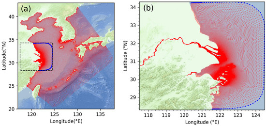
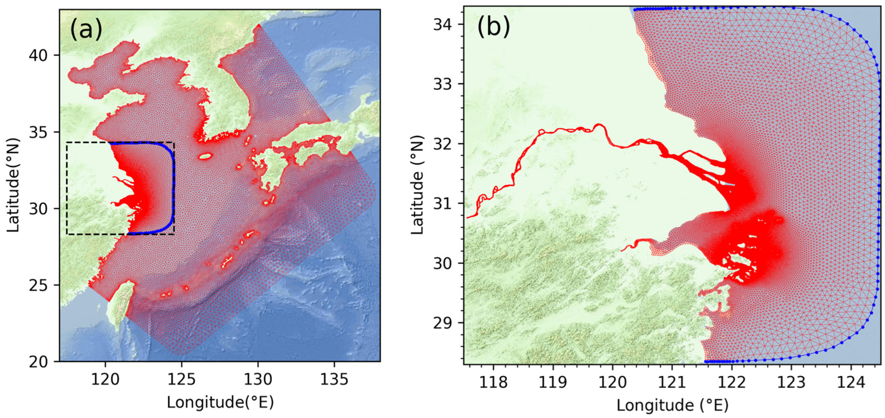
A two-domain nested SWAN model was developed for this study (Figure 2). The nested model consists of a shelf-scale ECS model (ECS-SWAN) and a regional YRD model (YRD-SWAN), with a one-way common-grid nesting procedure. The father ECS-SWAN model covers the whole ECS, from the Yellow Sea and Bohai Sea, to better capture the great waves induced by strong northerly winds in winter. The open boundary extends to the middle of the Japan Sea in the north, covering the whole Tsushima Strait, and to the northwest Pacific Ocean in the east to better capture swells from the Pacific Ocean. The horizonal resolution of the triangular grid is ~5 km along the coast and 30 km in the open boundary. Mesh is refined to ~0.5 km around the YRD. There are a total of 34,866 nodes and 64,280 triangular cells in the ECS-SWAN model. The computational domain of the child YRD-SWAN model covers the entire YRD, Hangzhou Bay and Zhoushan Archipelago and extends 124.5° E to the east. The mesh resolution is about 10 km in the open boundary and 200 m in the YRD coast on average. The computational grid consists of 50,098 nodes and 94,345 triangular elements.

Figure 2. Unstructured mesh grid of the two-domain nested SWAN model. (a) ECS-SWAN; (b) YRD-SWAN. The blue lines show the common grids for nesting.

The SWAN wave model offers multiple options in several key parameters and physical processes, including nonlinear interactions, wave breaking, whitecapping dissipation and bottom friction. Selection of these parameters and processes can significantly influence the model’s performance [33,34]. In this study, default settings of the nonlinear interactions and wave breaking parameters are adopted according to previous studies [32,35]. The KOMEN function is selected to calculate the wind input and whitecapping dissipation, following the recommendations of Jiang et al. [36] and Ma et al. [21], and JONSWAP bottom friction is employed with C_jon set to 0.038 m² s⁻³, as proposed by Jiang et al. [36]. The wave spectra are discretized over 32 frequencies (0.0521–1.0 Hz) and 24 directions.

The topography used in this SWAN model integrates 1-arc-minute ETOPO1 data [37] for offshore regions and a large number of high-resolution naval electronic nautical charts in coastal shallow waters. This study utilized the ERA5 10 m wind reanalysis data provided by the European Centre for Medium-Range Weather Forecasts (ECMWF) to drive the wave model [38]. The wind data feature a temporal resolution of 1 h and a spatial resolution of 0.25° × 0.25°. The simulation period spans from January 1993 to December 2023. The model outputs are available at 1-hour intervals. H_s and T_peak are extracted for the analysis of wave height and period.

2.2. In Situ Wave Buoys

Wave conditions from two in situ buoys are available for the YRD region, provided by the Shanghai Municipal Oceanic Bureau. Locations of the buoys are shown in Figure 1b. The Hs and mean wave period (T_mean) records for one summer month and one winter month (July and December 2021) are collected for the validation of our SWAN model.

2.3. Calculations

2.3.1. Error Metrics

Three skill metrics are adopted to evaluate the SWAN model’s performance, including the root-mean-square error (RMSE), Willmott model skill score (WS), relative error (RE), bias, correlation coefficient (R) and scatter index (SI). Their calculation formulas are as follows:

$$\mathrm{R}\mathrm{M}\mathrm{S}\mathrm{E}=\sqrt{{\displaystyle \frac{1}{N}}\sum _{i=1}^N {\left(X_m-X_o\right)}^2} ,$$

(3)

$$\mathrm{W}\mathrm{S}=1-{\displaystyle \frac{{\left(X_m-X_o\right)}^2}{{\left(\left|X_m-\overline{X_0}\right|+\left|X_o-\overline{X_0}\right|\right)}^2}} ,$$

(4)

$$\mathrm{R}\mathrm{E}={\displaystyle \frac{\frac{1}{N}{\displaystyle {\sum }_{i=1}^N} \left|X_{m,i}-X_{o,i}\right|}{max\left(X_o\right)-min\left(X_o\right)}}\times 100\%,$$

(5)

$$\mathrm{B}\mathrm{i}\mathrm{a}\mathrm{s}={\displaystyle \frac{1}{N}}\sum _{i=1}^N (X_m-X_o) ,$$

(6)

$$\mathrm{R}={\displaystyle \frac{{\displaystyle {\sum }_{i=1}^N} (X_m-\overline{X_m})(X_o-\overline{X_0})}{\sqrt{{\displaystyle {\sum }_{i=1}^N} (X_m-{\overline{X_m})}^2}\sqrt{{\displaystyle {\sum }_{i=1}^N} (X_o-\overline{X_0}{)}^2}}} ,$$

(7)

$$\mathrm{S}\mathrm{I}={\displaystyle \frac{RMSE}{\overline{X_0}}} ,$$

(8)

where X represents the statistical variable (such as H_s and T_mean), N is the number of samples involved in the comparison, $\overline{X}$ is the average value of the samples, the subscript m denotes model results, and the subscript o represents observed data.

2.3.2. Trend Detection

This study analyzed the wave hindcast in the YRD and adjacent waters from 1993 to 2023, mainly focusing on H_s and T_peak. The average values, maximum values, and 90th percentile values of the two parameters over two different time scales (seasonal and annual) were calculated. Linear regression was used to detect the long-term trends of H_s and T_peak over different time series, and the Mann–Kendall (M-K) test was applied to test the significance. The p-value for correlation was obtained through calculation, and trends with p-value < 0.05 were considered statistically significant.

2.3.3. Variability

This study employs interannual variability (IAV) to analyze the interannually varying amplitude of wave parameters during the 1993–2023 period. It is calculated by dividing the standard deviation of specific parameters over the 31-year period by their multi-year mean. The calculation formula is as follows:

$$S_x=\sqrt{{\displaystyle \frac{1}{n}}\sum _{i=1}^n {\left(x_i-\overline{x}\right)}^2} ,$$

(9)

$$\mathrm{I}\mathrm{A}\mathrm{V}={\displaystyle \frac{S_x}{\overline{x}}} ,$$

(10)

where S_x denotes the standard deviation, n represents the total number of years, and $\overline{X}$ stands for the multi-year mean. The IAV is a dimensionless parameter. Thus, it can compare interannual fluctuations across areas with different wave conditions.

3. Results and Discussions

3.1. SWAN Model Validation

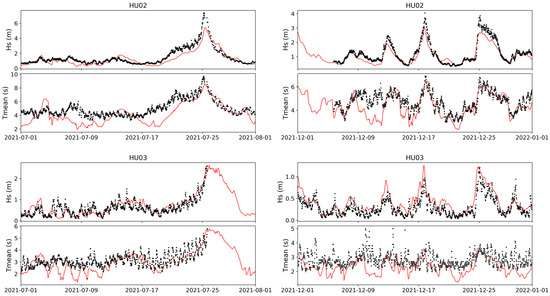
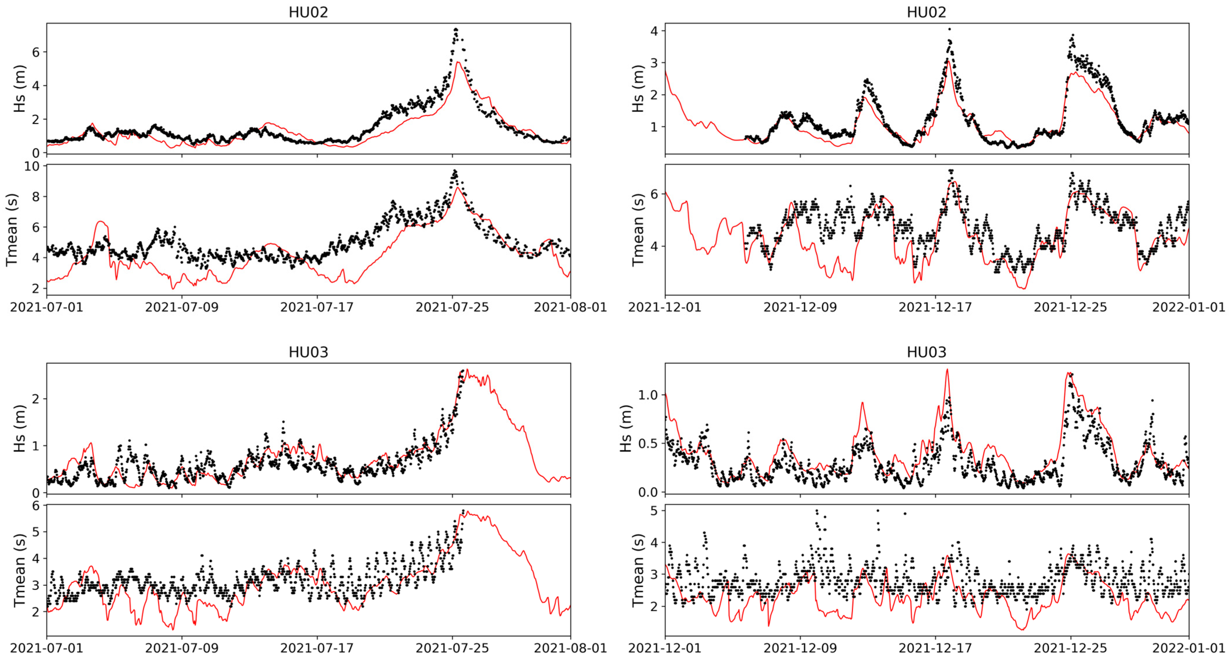
Figure 3 displays a comparison of the SWAN hindcast and measured hourly H_s and T_mean at two wave buoys during July and December 2021. It is obvious that the hindcast wave parameters are in good agreement with the measurements for both buoys. The two-domain SWAN model can reproduce the temporal oscillation in measurements well and fully captures the strong wave events. The error metrics are presented in Table 1. The average RMSEs for H_s are 0.405 m and 0.24 m, and the average RMSEs for T_mean are 1.005 s and 0.82 s. The average WS values for H_s are 0.91 and 0.905, the average bias values are −0.09 m and −0.025 m, and the average R values are 0.85 and 0.89. The skills are comparable with those of other studies near the YRD, such as Luo et al. [30]. Overall, the hindcast waves of the SWAN model are in good agreement with the measurements, indicating that our SWAN model can effectively simulate the wave field in the YRD and adjacent waters.

Figure 3. Comparison of H_s and T_mean between SWAN hindcast (red) and buoy measured data (black) at HU02 and HU03 in July (left) and December (right) 2021.

Table 1. Error metric comparison between SWAN hindcast with observations at two buoys in July and December 2021.

		Hs						Tmean
		RMSE (m)	WS	RE	Bias (m)	R	SI	RMSE (s)	WS	RE	Bias (s)	R	SI
July	HU02	0.57	0.92	6.20%	−0.21	0.89	0.38	1.31	0.75	16.60%	−0.8	0.71	0.26
	HU03	0.24	0.9	7.30%	0.03	0.81	0.4	0.7	0.71	16.40%	−0.32	0.61	0.22
	Average	0.405	0.91	6.75%	−0.09	0.85	0.39	1.005	0.73	16.50%	−0.56	0.66	0.24
December	HU02	0.31	0.95	6.20%	−0.15	0.95	0.25	0.84	0.79	16.00%	−0.44	0.7	0.18
	HU03	0.17	0.86	11.30%	0.1	0.83	0.58	0.8	0.49	20.80%	−0.52	0.26	0.28
	Average	0.24	0.905	8.75%	−0.025	0.89	0.415	0.82	0.64	18.40%	−0.48	0.48	0.23

3.2. General Characteristics of H_s and T_peak

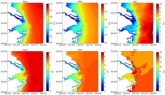
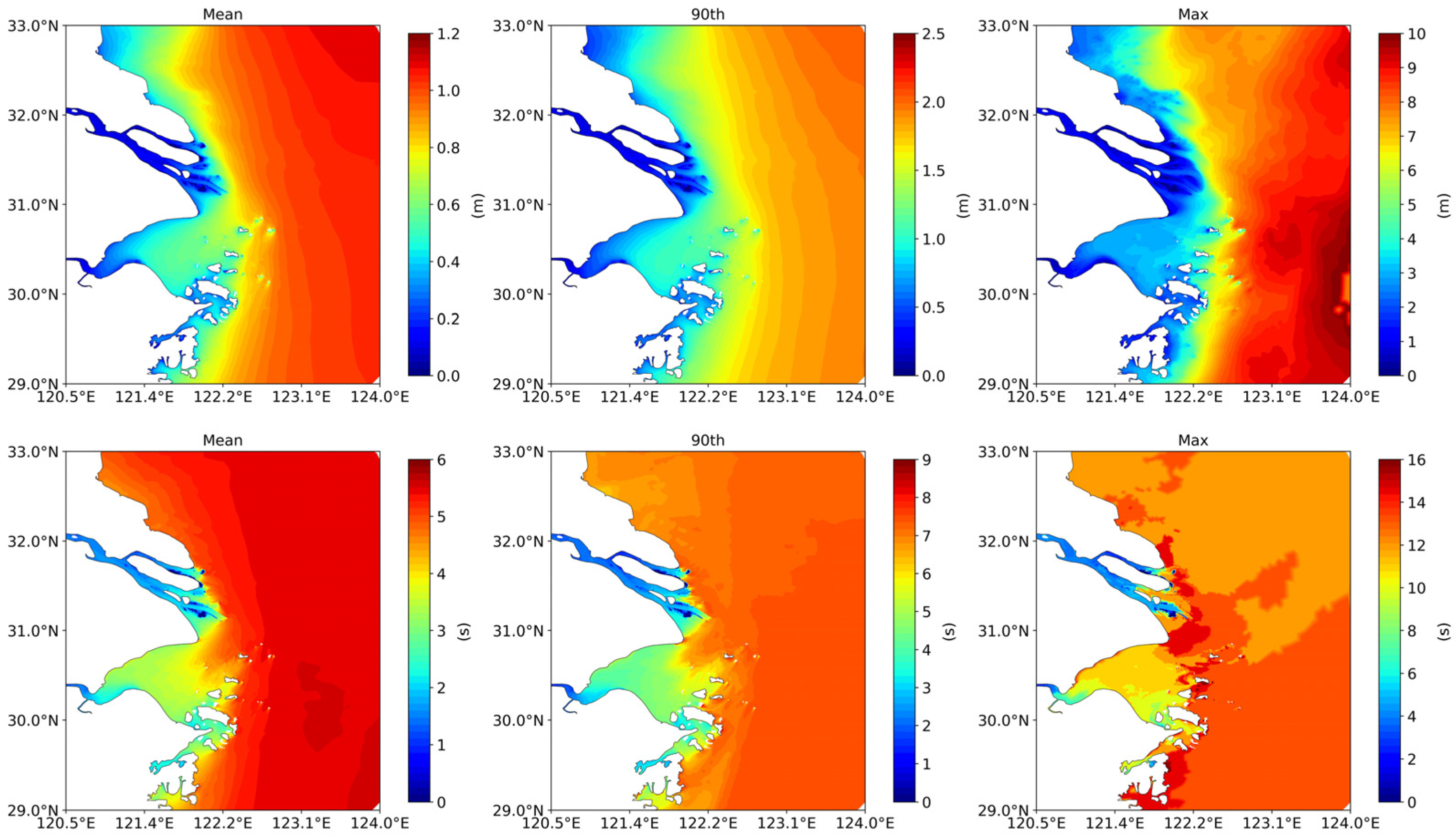
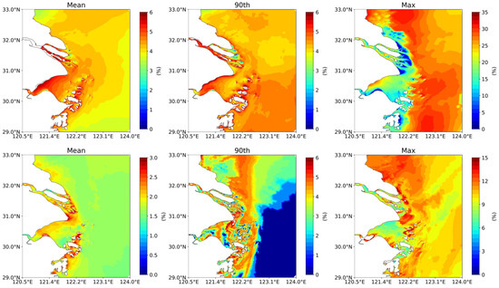
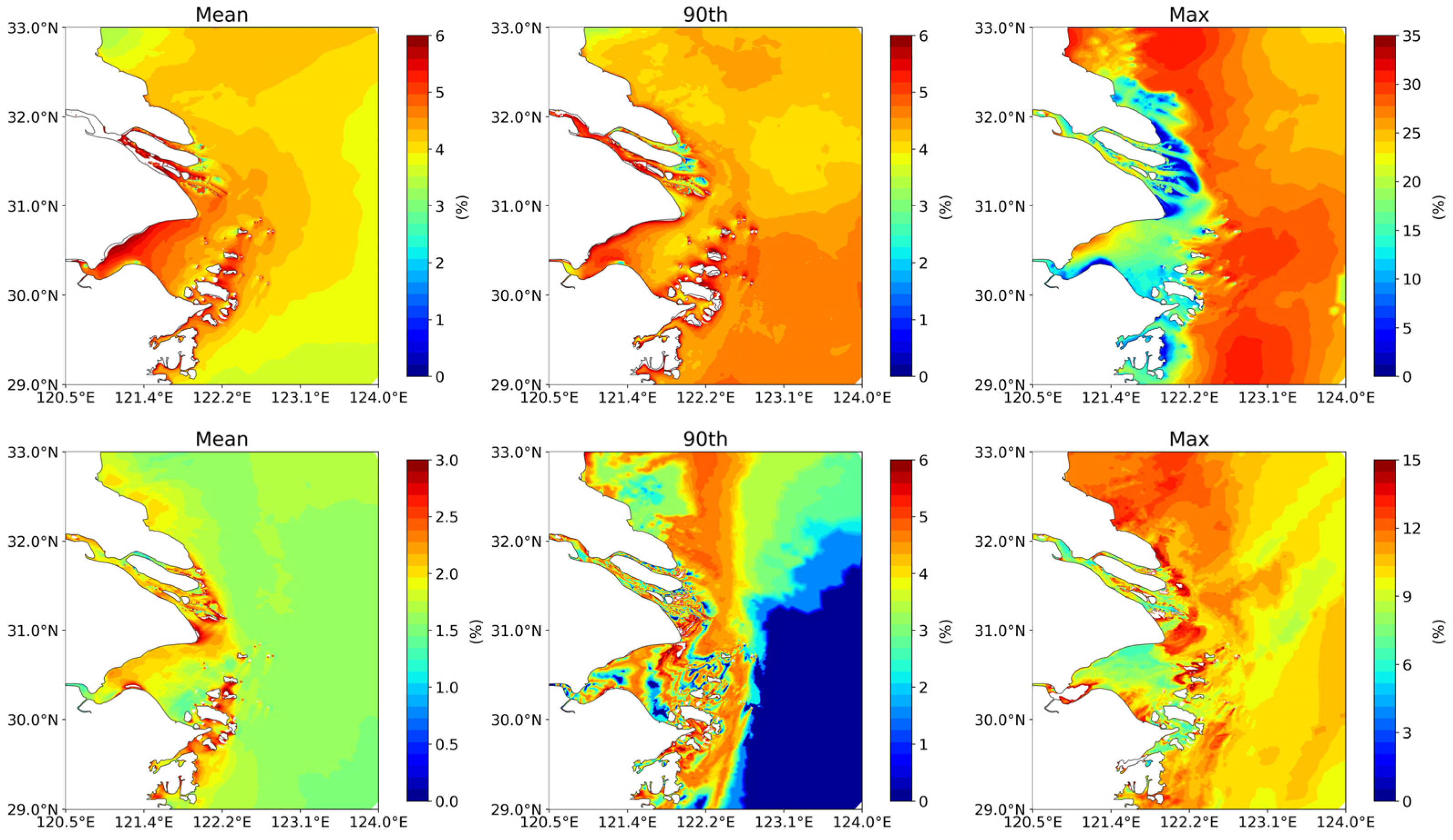
Figure 4 shows the spatial distributions of the means, 90th percentiles and maxima of H_s and T_peak over the period of 1993–2023. It is obvious that H_s values are significant in deep waters and decrease remarkably toward shallow coastal areas. H_s values are especially weak in the Yangtze River Estuary. The area-mean H_s,mean values in the Hangzhou Bay and YRD are 0.42 and 0.88 m, respectively, which are notably smaller than in the northwestern ECS (1.03 m) and southern Yellow Sea (0.90 m). The regional average values of the three indicators for H_s across the entire study area are H_s,mean = 0.86 m, H_s,90 = 1.54 m, and H_s,max = 6.75 m. The spatial distributions exhibit inconsistency between different indicators. H_s,mean and H_s,90 are higher in the southern Yellow Sea (about 0.89 m and 1.57 m) but smaller in the ECS, while H_s,max in the ECS (about 9.16 m) is significantly higher than in the southern Yellow Sea (about 6.64 m). This difference is highly influenced by the fact that typhoons always pass through the ECS but rarely pass through the southern Yellow Sea.

Figure 4. Spatial distributions of the means, 90th percentiles and maxima of H_s (upper) and T_peak (lower) in the YRD and adjacent waters over the 1993–2023 period. Please note the different color scales.

The regional average values for T_peak are T_peak,mean = 5.05 s, T_peak,90 = 6.85 s and T_peak,max = 12.31 s. All the three indicators show a distinct south–north difference of being longer in the ECS and shorter in the southern Yellow Sea. T_peak also exhibits relatively smaller values in the shallow Hangzhou Bay and Yangtze River Estuary. An exception occurs for T_peak,max, for which a high value is observed in the conjunction of the YRD and Hangzhou Bay, which was induced by a strong typhoon, Muifa (1109), that passed through the middle of the ECS and the Yellow Sea in 2011. In addition, T_peak values have less spatial variance compared with H_s.

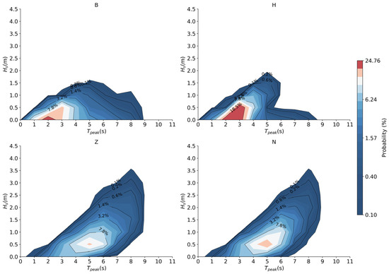
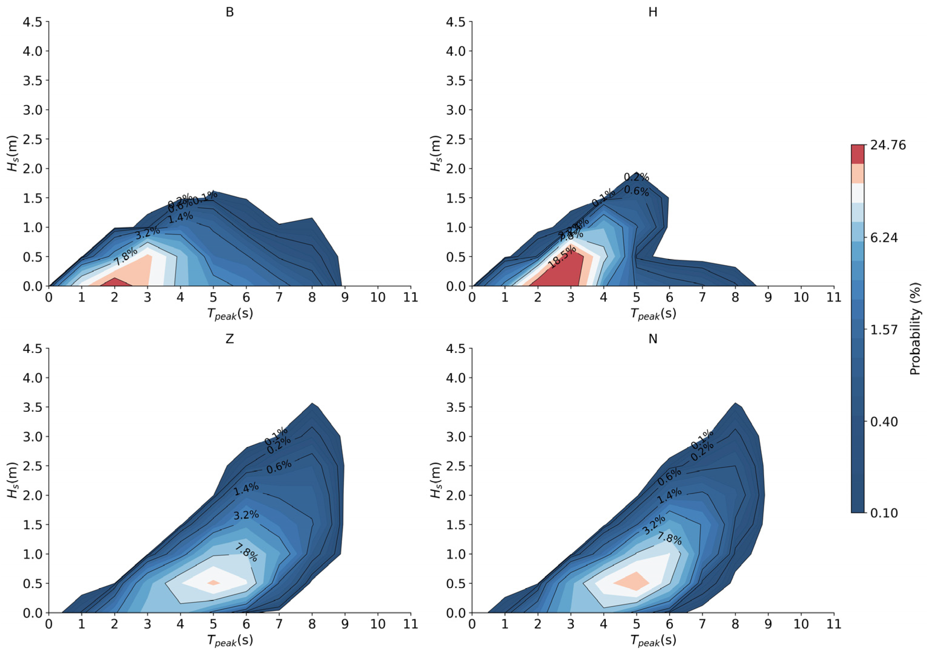
The joint distribution of H_s and T_peak are further analyzed at four selected stations, as shown in Figure 1. Stations B, H, Z and N are located in the YRD, Hangzhou Bay, ECS and southern Yellow Sea, respectively. Their results are presented in Figure 5. At station B, waves with H_s of 0–0.5 m and T_peak of 2–3 s have the highest probability density, accounting for 46.43% and 24.14%, respectively. There are 70% waves with a T_peak of less than 4 s. At station H, waves with H_s of 0.5–1 m and T_peak of 3–4 s have the highest frequency of 24.76%. These characteristics imply that the waves in YRD and Hangzhou Bay are predominantly mild wind-waves.

Figure 5. Joint frequency distribution diagram of H_s and T_peak.

At the two offshore stations (N and Z), the highest probability density happens with a longer T_peak (~5 s) and stronger H_s (0.5–1 m). At N and Z, the proportions of waves with a T_peak exceeding 6 s are 35.7% and 39.3%, respectively, while the proportions of waves with H_s exceeding 1 m are 15.3% and 15.9%, respectively, indicating a higher frequency of swells and high waves in these two areas. In addition, the joint distributions of the two offshore stations (N and Z) are more dispersed, especially during high waves. These characteristics indicate that the waves in the offshore ECS and southern Yellow Sea are predominantly a mixture of wind-waves and swells.

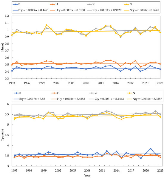
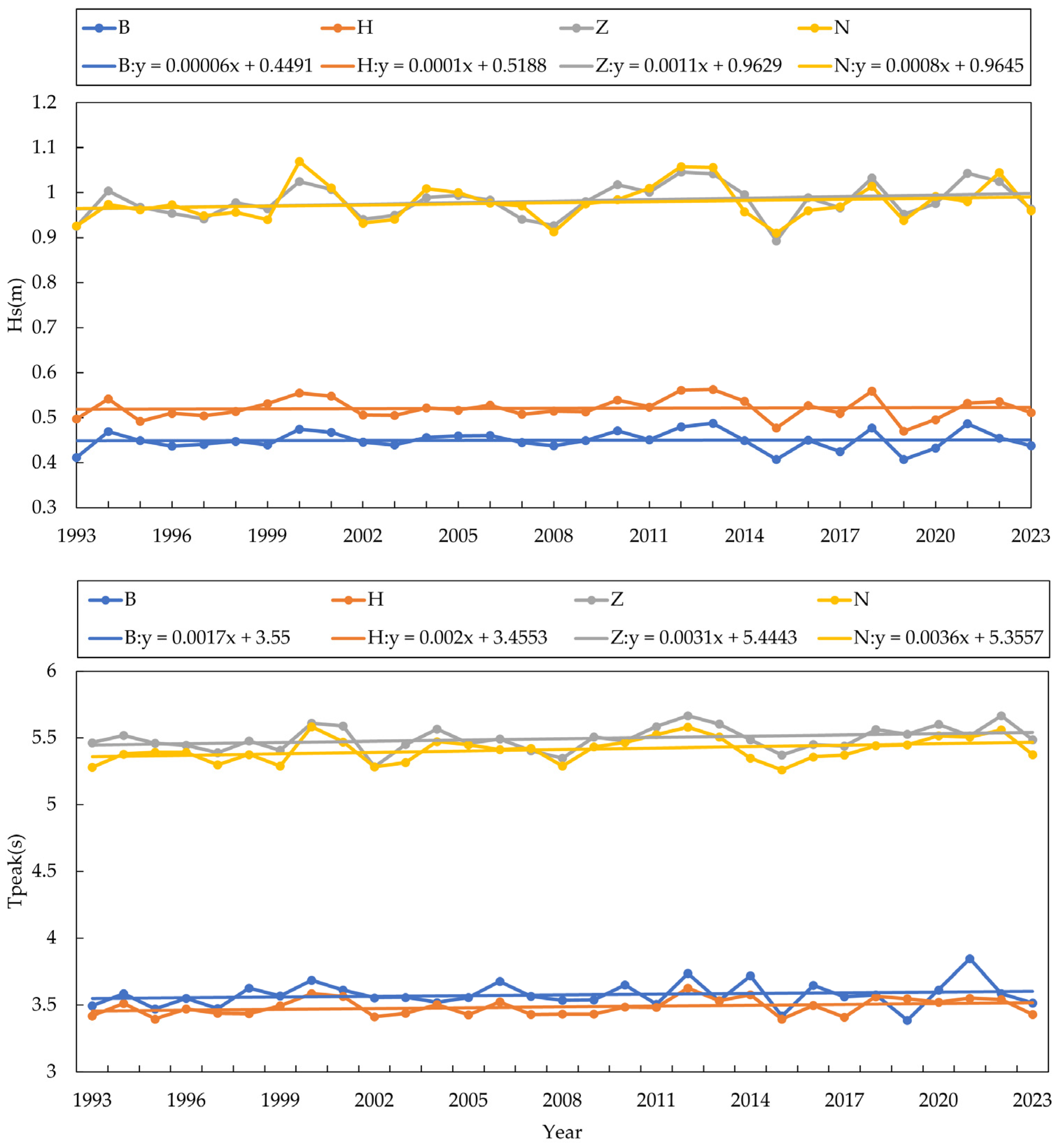
The wave parameters at the four stations were averaged annually from 1993 to 2023 to analyze the variation trends of waves in different regions. As shown in Figure 6, the waves at all four stations show a trend of increasing year by year, with the growth trends of the two offshore stations being greater than those of the two coastal stations. At stations B and H, the trends of H_s and T_peak are 0.006 cm a⁻¹ and 0.01 cm a⁻¹ and 0.0017 s a⁻¹ and 0.002 s a⁻¹, and the variation trends of the coastal stations are relatively gentle. At stations N and Z, the trends of H_s and T_peak are 0.08 cm a⁻¹ and 0.11 cm a⁻¹ and 0.0031 s a⁻¹ and 0.0036 s a⁻¹, respectively.

Figure 6. Interannual variations in H_s and T_peak at four stations during the 1993–2023 period.

3.3. Intra-Annual Variability

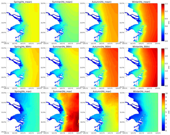
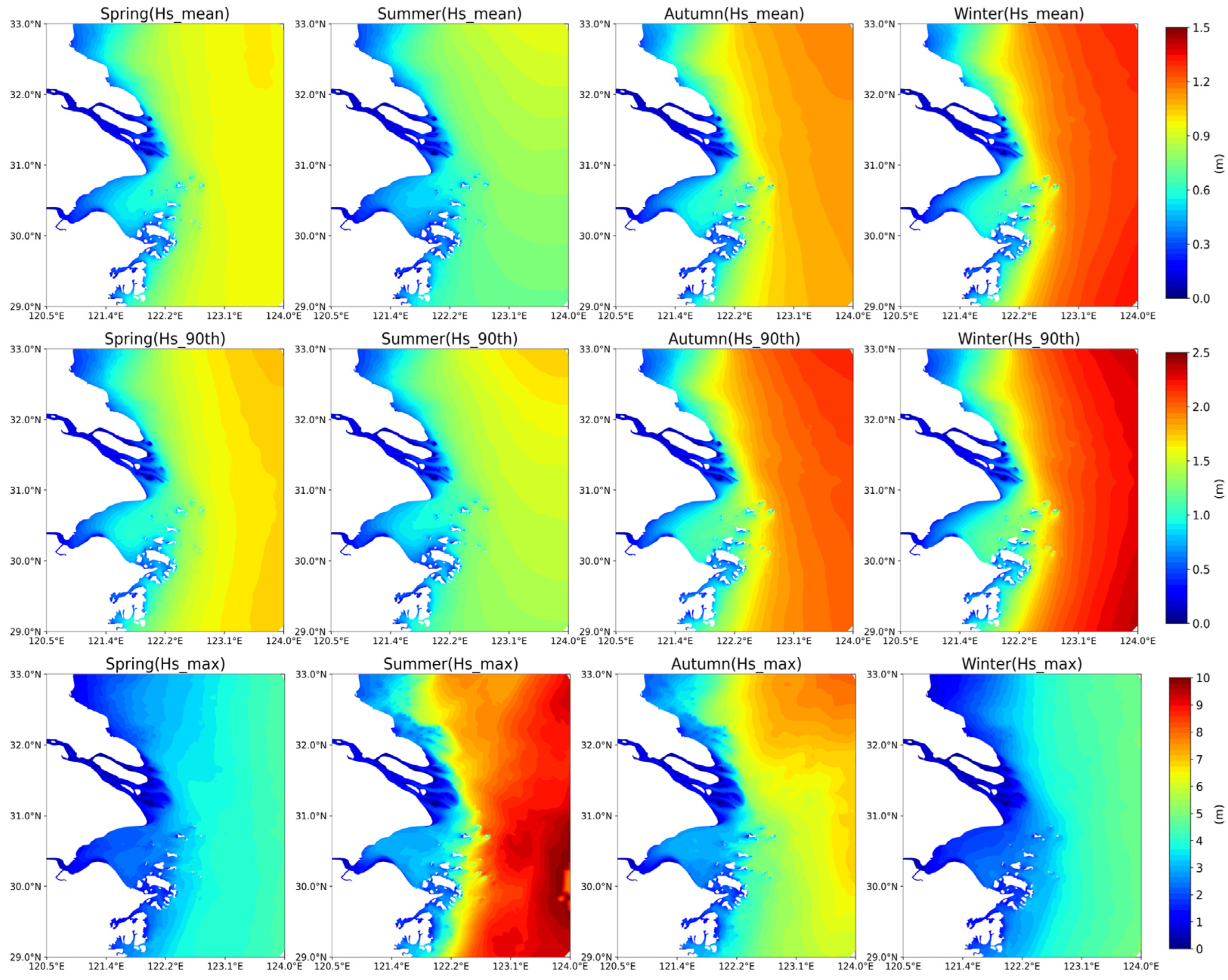
Figure 7 displays the spatial distributions of the mean, 90th percentile, and maximum values of H_s across four seasons over the period of 1993–2023. In this study, we define March–April–May as spring, June–July–August as summer, September–October–November as autumn, and December–January–February as winter. It is obvious that H_s,mean and H_s,90 are somewhat higher in winter and autumn, but H_s,max is much higher during summer, followed by autumn. This feature implies that the climatology-mean wave condition is strongly influenced by the frequent cold-air-induced high winds in winter, controlled by Asian monsoons, while extreme waves are controlled by typhoon events, which always occur in summer and autumn.

Figure 7. Seasonal variations in the mean (upper), 90th percentile (middle), and maximum (lower) values of H_s in the YRD and adjacent waters during the 1993–2023 period. We defined spring as March–April–May (MAM), summer as June–July–August (JJA), autumn as September–October–November (SON), and winter as December–January–February (DJF). Please note the different color scales.

The spatial distribution of H_s also varies seasonally. H_s,mean and H_s,90 maintain a distinct spatial pattern of “relatively high in the southern Yellow Sea but weaker in the ECS” in spring, summer, and autumn, but there is less north–south discrepancy in winter. This spatial pattern can be attributed to the dominant role of Asian monsoons, which produce northerly high wind during winter and relatively mild winds in other seasons. H_s,max is higher in the ECS during the summer season, indicating the influence of typhoons, but the reverse is true in the autumn, and there is less north–south discrepancy in winter. The winter northerly strong wind occurs more frequently in the southern Yellow Sea, and typhoons pass through the ECS more frequently. The combination of the two results in a discrepancy between the spatial patterns of the mean and maximum wave conditions, as Figure 4 shows, i.e., H_s,mean is higher in the southern Yellow Sea and H_s,max is higher in the ECS. The YRD is located in the junction between the southern Yellow Sea and ECS and is significantly affected by both winter northerly strong winds and typhoons.

In addition, the sheltering effect of the Zhoushan Archipelago is clearly illustrated in Figure 7. During the summer season, H_s,max values in the Hangzhou Bay (about 2.48 m) are much smaller than in the ECS (about 9.16 m), reflecting that the Zhoushan Archipelago protects the Hangzhou Bay from extreme waves.

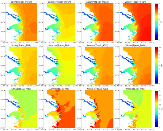
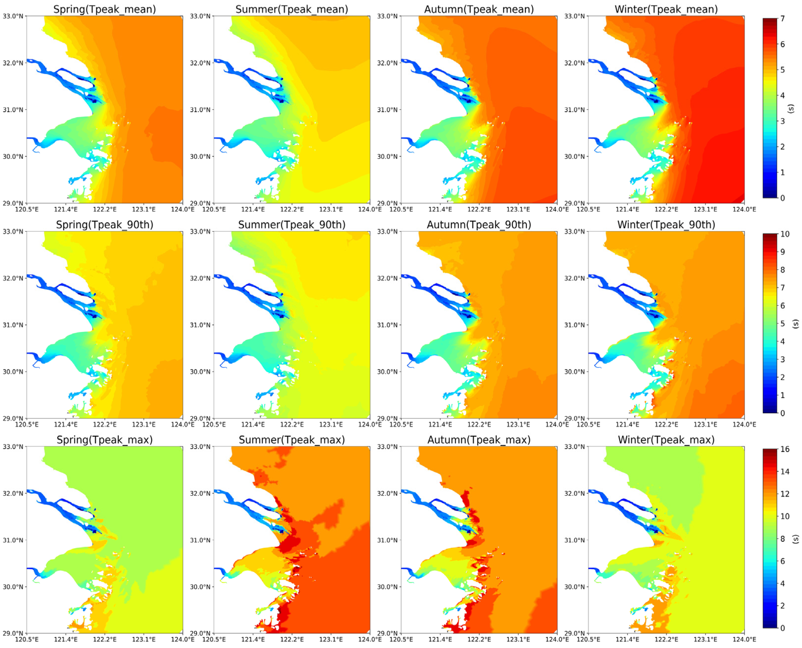
Correspondingly, the T_peak indicates that T_peak,mean and T_peak,90 are higher in winter (about 5.51 s and 7.06 s) and autumn (about 5.24 s and 6.96 s), while T_peak,max is considerably higher during summer (about 12.24 s) and autumn (about 11.69 s) than during spring (about 9.17 s) and winter (about 9.56 s) (Figure 8). Although the spatial pattern of “longer in the ECS but shorter in southern Yellow Sea” holds true in most situations, it is mostly reversed during summer, especially for T_peak,mean and T_peak,90. A simple understanding relates to the fetch length. Specifically, the prevailing direction of summer waves is northward or northwestward. The longer fetch of the southern Yellow Sea leads to longer wave periods.

Figure 8. Seasonal variations in the mean (upper), 90th percentile (middle), and maximum (lower) values of T_peak in the YRD and adjacent waters during the 1993–2023 period. Please note the different color scales.

3.4. Interannual Fluctuation

We use IAV, which is calculated using Equations (6) and (7), to quantify the interannual fluctuation of wave parameters. The IAVs of H_s and T_peak are displayed in Figure 9. It is obvious that the IAV values are smaller for the mean and 90th percentiles of H_s and T_peak but significantly larger for the maximum. Across the entire study area, the IAVs of H_s,mean and H_s,90 are 4.2% and 4.4%, respectively, but they increase considerably to 24.8% for H_s,max. The IAVs of T_peak,mean and T_peak,90 are 1.7% and 2.4%, respectively, and they also increase remarkably to 10.5% for T_peak,max.

Figure 9. Interannual variability (IAV) of the mean, 90th percentile and maximum values of H_s (upper) and T_peak (lower) in the YRD and adjacent waters during 1993–2023 period. Please note the different color scales.

Figure 9 also show that regions with relatively small H_s,mean and T_peak,mean, such as in the Yangtze River Estuary, Hangzhou Bay and the Zhoushan Archipelago, exhibit larger IAVs, while offshore regions with larger H_s,mean and T_peak,mean show relatively smaller IAVs. For the 90th percentiles, the H_s,90 shows a nearly spatially uniform pattern of slightly higher values in the ECS than in the southern Yellow Sea. T_peak,90 shows a spatial pattern similar to T_peak,mean, with large waves in shallow waters but small ones deep waters, with greater diversity. These features imply that the mean statistical features of waves in deep waters are more annually stable. In addition, it should be noted that the IAVs of H_s,mean and T_peak,mean are extremely high between the islands in the Zhoushan Archipelago, embodying the sheltering effect of the islands.

For the annual maximums, the IAVs of H_s,max and T_peak,max are larger in deep waters and smaller in shallow waters. This is mainly because rare extreme events can result in extreme waves in deep waters, while shallow waters will restrict the development of extreme waves.

Previous studies indicated that variations in surface ocean waves are related to both atmospheric and oceanic climate indexes [6,7]. The common used climate oscillations include ENSO, PDO, Atlantic Multidecadal Oscillation (AMO), Indian Ocean Dipole (IOD), Arctic Oscillation (AO) and Antarctic Oscillation (AAO) [6,7,39,40]. In the ECS, Wang et al. [17] reported that the mean condition of wind waves was significantly influenced by ENSO and PDO, with a negative correlation. Both ENSO and PDO were also confirmed to have significant impacts on extreme waves in this region [41], since the occurrence of El Niño can induce longer and more intense summer extreme waves, and a positive PDO tends to enhance this effect.

Accordingly, the impacts of ENSO and PDO on the wave parameters in the YRD and adjacent area were examined in this study. Additionally, the Western Pacific Subtropical High Ridge Position (WPSH) Index was also taken into account (downloaded from https://cmdp.ncc-cma.net/cn/monitoring.htm, accessed on 14 January 2026).

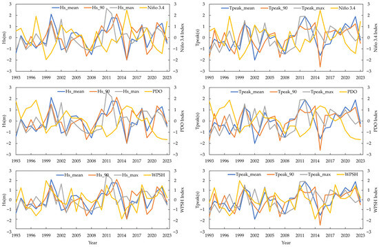
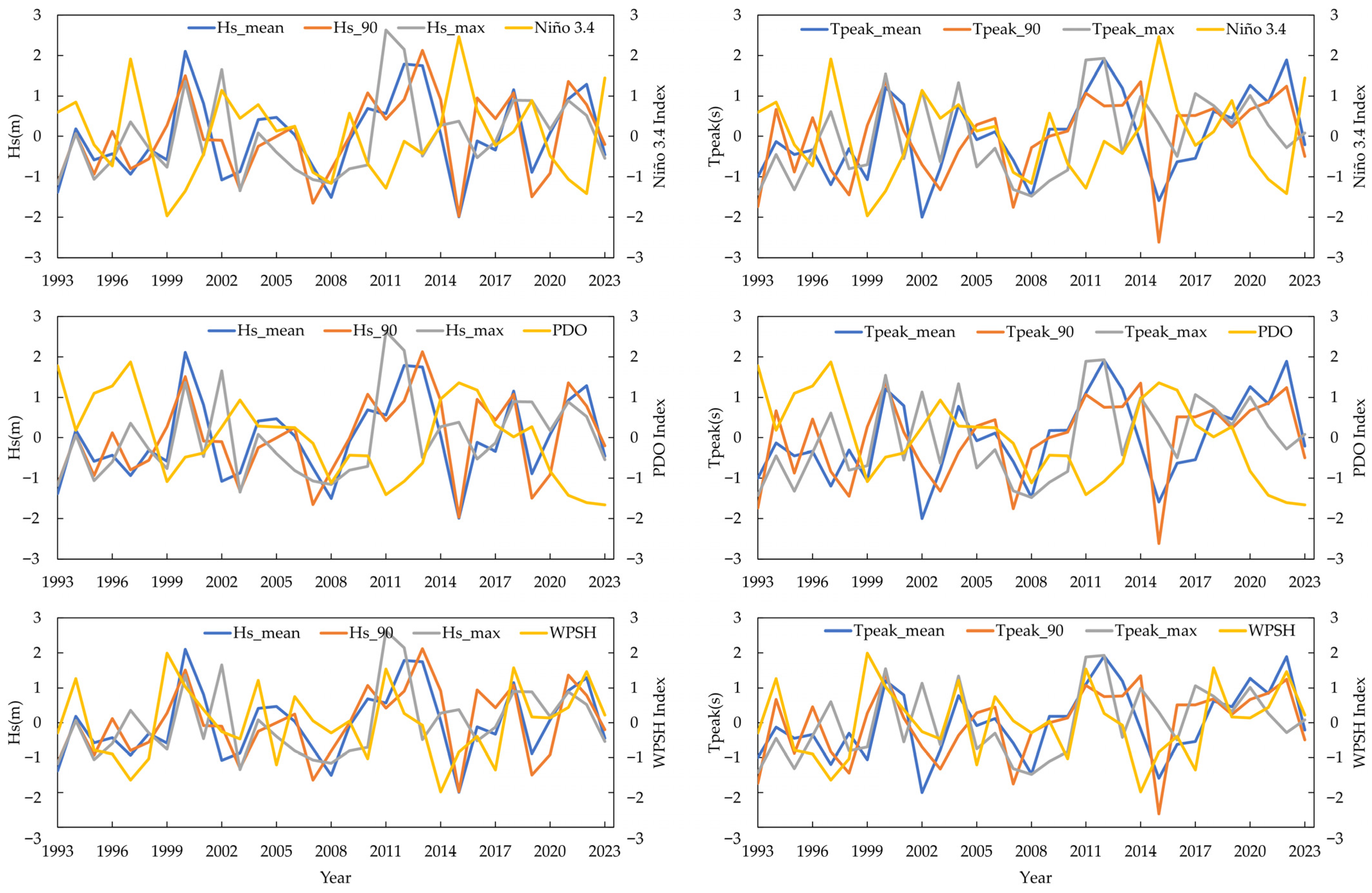
After processing the monthly average data of the aforementioned indicators into annual average data, we performed z-score standardization to normalize the wave parameters and climate indices ($z={\displaystyle \frac{x-\overline{x}}{std\left(x\right)}}$). The results of a comparison with the three climate indexes are displayed in Figure 10, and their statistical correlations are summarized in Table 2. Except for the positive correlation of T_peak,max with the Niño 3.4 index, both the mean and extreme values of H_s and T_peak are negatively correlated with the Niño 3.4 index and PDO index, which confirms the findings by Wang et al. [17] and Bayhaqi et al. [41], although the correlations of the maximal values are weak. Further, the wave parameters are positively correlated with the WPSH index. A higher WPSH index indicates a higher latitude of the WPSH Ridge Position, which favors northward movement of typhoons, resulting in a stronger impact of typhoons on the YRD and adjacent waters.

Figure 10. Correlations between the mean values, 90th percentile values and maximum values of H_s and T_peak and the Niño 3.4 Index (upper), PDO Index (middle) and WPSH Index (lower).

Table 2. Correlations between different values of H_s and T_peak and the Niño 3.4 Index, PDO Index and WPSH Index.

	Niño 3.4	PDO	WPSH
Hs,mean	−0.46	−0.51	0.40
Tpeak,mean	−0.42	−0.56	0.45
Hs,90	−0.42	−0.41	0.24
Tpeak,90	−0.50	−0.48	0.34
Hs,max	−0.01	−0.29	0.30
Tpeak,max	0.09	−0.17	0.18

3.5. Long-Term Trends

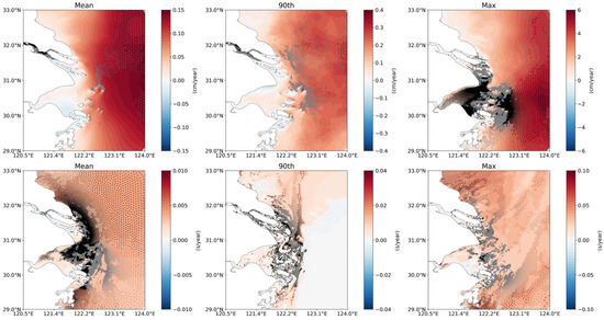
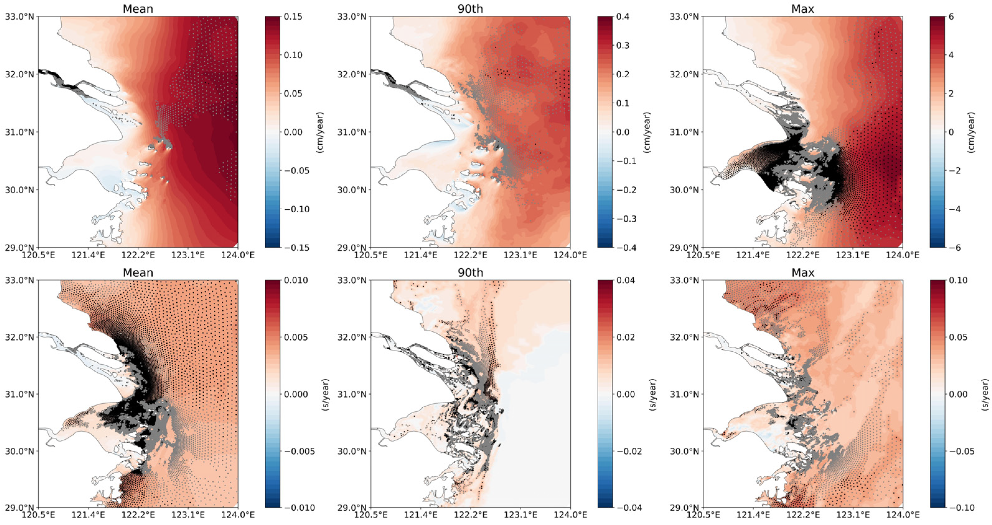
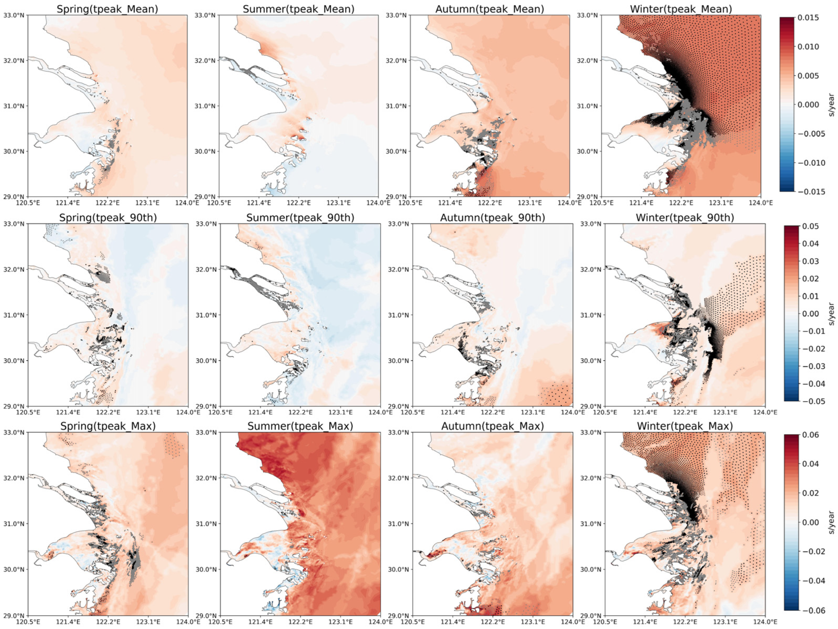
The long-term trends of H_s and T_peak were determined by applying a linear regression model on annual data for the 1993–2023 period. The spatial distributions of these trends are shown in Figure 11 for all annual data and in Figure 12 and Figure 13 for the different seasons. The black and gray dots indicate regions where the trends are statistically significant at the 95% and 90–95% confidence levels after the Mann–Kendall test.

Figure 11. Long-term trends of the annual mean, 90th percentile, and maximum values of H_s (upper) and T_peak (lower) in the YRD and adjacent waters from 1993 to 2023. Black and gray dots indicate regions where the trends are statistically significant at the 95% and 90–95% confidence levels after the Mann–Kendall test. Please note the different color scales.

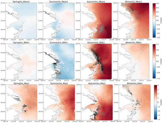
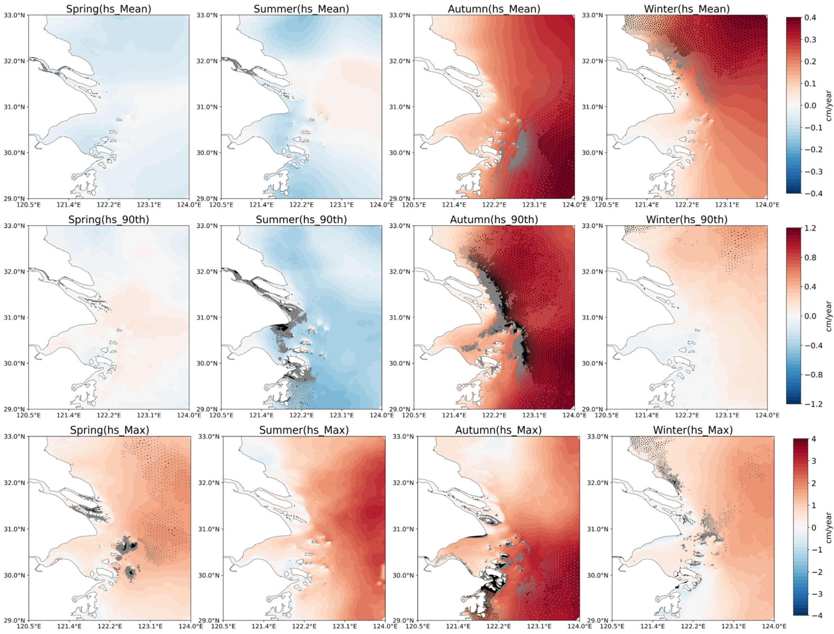
Figure 12. Trends of the seasonal mean (upper), 90th percentile (middle), and maximum (lower) of H_s in the YRD and adjacent waters from 1993 to 2023. Black and gray dots indicate regions where the trends are statistically significant at the 95% and 90–95% confidence levels after the Mann-Kendall test. Please note the different color scales.

Figure 13. Trends of seasonal mean (upper), 90th percentile (middle) and maximum (lower) values of T_peak in the YRD and adjacent waters from 1993 to 2023. Black and gray dots indicate regions where the trends are statistically significant at the 95% and 90–95% confidence levels after the Mann–Kendall test. Please note the different color scales.

As Figure 11 shows, the annual trends tend to be positive in most of the areas for the mean, 90th percentile and maximum values of H_s and T_peak, implying a potential positive trend of wave conditions. The positive trends are stronger for extreme conditions than that of mean conditions. The regional-mean increasing rate for H_s,max is ~2.87 cm a⁻¹, which is significantly faster than the ~0.09 cm a⁻¹ for H_s,mean. The growth rates are ~1 cm a⁻¹ different to those reported by relatively coarse models with larger domains [17,30], showing the importance of applying a high-resolution model in assessing the wave height and period of coastal areas. Similarly, the regional-mean increasing rate of T_peak,max (0.03 s a⁻¹) is also significantly faster than the growth rate of T_peak,mean (0.003 s a⁻¹). For H_s, the magnitude of the long-term positive trend is considerably larger in offshore deep waters, whereas it is noticeably smaller in the shallow Hangzhou Bay and the Yangtze River Estuary. Similar spatial pattern exist for the mean and maximum of T_peak but not for the 90th percentile of T_peak, in which a potential negative trend is observed in the deep ECS.

The long-term trends are statistically significant (p < 0.05) in the Hangzhou Bay, inner YRD and ECS for H_s,max with regional-mean values of 1.31, 0.72 and 4.14 cm a⁻¹, respectively. The prominent discrepancy in the growth rate between regions further highlights the importance of coastal wave height and period assessment with high-resolution models. Nevertheless, this result is consistent with the reported weak positive trend of extreme waves in the ECS, which is relating to changes in typhoon climatology [30]. For the T_peak, the long-term trends are statistically significant (p < 0.05) in the southern Yellow Sea, YRD and northern Hangzhou Bay for T_peak,mean, with values of about 0.0039, 0.0037 and 0.0022 s a⁻¹, respectively, and significant between the islands in the Zhoushan Archipelago, with increasing rate of about 0.0027 s a⁻¹.

Figure 12 illustrates that the long-term trends in H_s differ between seasons. There are no distinct (or slightly negative, spring: −0.12~0 cm a⁻¹; summer: −0.161~0 cm a⁻¹) trends (p > 0.1) in H_s,mean during spring and summer, but remarkable positive trends exist in autumn (0.23 cm a⁻¹) and winter (0.19 cm a⁻¹). This seasonal discrepancy is consistent with the SWAN results of Ma et al. [21]. For the ECS and southern Yellow Sea in particular, the positive trends are statistically significant (p < 0.05) in autumn and winter, respectively, while for H_s,max, the whole region shows a positive trend, with distinct shifts in peak locations. Specifically, the peaks are located at the outer YRD and the southern Yellow Sea in spring and summer, with values of up to 1.825 cm a⁻¹ in spring and 3.212 cm a⁻¹ in summer, but they shift southward to the ECS in autumn and turn northward to the southern Yellow Sea in winter, with values of up to 3.8 cm a⁻¹ and 1.93 cm a⁻¹. For the H_s,90, the opposite trend occurs between summer and autumn. H_s,90 shows a statistically significant positive trend, with a regional-mean value of 0.74 cm a⁻¹ in autumn and a distinct, slightly negative trend in summer of about −0.31 cm a⁻¹, although these trends are not statistically significant (p > 0.1).

In general, the autumn season experiences the most remarkable positive trends of H_s, which may be related to the increasing number and intensity of typhoons in autumn [42]. The winter season is also characterized by remarkable increasing trends of H_s, especially in the southern Yellow Sea. The H_s trends in spring are always not remarkable, but the H_s trends in summer are chaotic, with potential positive trends in H_s,max but negative trends in H_s,90, although none are statistically significant (p > 0.1).

Figure 13 displays the seasonal trends in T_peak. It is obvious that the trends in T_peak,mean are slight and not statistically significant (p > 0.1) in spring and summer (spring: −0.006~0.01 s a⁻¹; summer: −0.008~0.013 s a⁻¹), becoming much more significant for autumn and winter, with values of up to 0.015 s a⁻¹. During winter in particular, the trends are statistically significant in most areas, including the southern Yellow Sea, YRD, the northern Hangzhou Bay and the Zhoushan Archipelago (p < 0.1). The magnitudes of trends in T_peak,90 are much slighter. Although slight, they are statistically significant in some areas of the YRD. In addition, large-scale negative trends (not statistically significant) are observed for summer T_peak,90, corresponding to the decreasing summer H_s,90. For T_peak,max, although the trends are greater in summer (regional-mean of 0.026 s a⁻¹), they are not statistically significant (p > 0.1). The regional-mean trends of T_peak,max in winter are slightly weaker (about 0.015 s a⁻¹), but they are statistically significant in most areas of the southern Yellow Sea and the YRD (p < 0.05).

4. Conclusions

In this study, a high-resolution two-domain numerical wave model based on the third-generation wave model SWAN is established for the YRD and adjacent waters. The model domain covers the YRD, Hangzhou Bay, Zhoushan Archipelago, southern Yellow Sea and part of the ECS. After careful validation, this model is adopted to hindcast wave conditions for 31 successive years (1993–2023), which may be used for maritime and coastal engineering applications in this region. Analysis of the 31-year wave database reveals some characteristics of H_s and T_peak.

(1)

Remarkable inconsistencies exist in the mean and extreme wave conditions, including their spatial distribution and seasonal variation. The main mechanism responsible for these discrepancies is the predominant influence of Asian monsoons, with strong winter winds and mild summer winds, on the wave mean conditions, but typhoon events, which always occur in summer and autumn, control the extreme wave conditions. The different dominant mechanisms result in a larger H_s,mean in the southern Yellow Sea compared to the ECS, but the reverse is true for H_s,max; and higher H_s,mean in winter due to the monsoon and much higher H_s,max in summer. There are also inconsistencies in T_peak. The prevailing northerly strong wind during winter induces longer T_peak,mean in the ECS with longer fetch and vice versa for the summer season.

(2)

We also analyzed the correlations between wave parameters and climate indices (the Niño 3.4 index, the PDO Index and the WPSH Index) Both the mean values and the 90th percentile values of H_s and T_peak showed positive correlations with the WPSH index but negative correlations with the Niño 3.4 index and PDO index. The maximum values exhibited slight differences: T_peak,max showed a weak positive correlation with the Niño 3.4 index. A higher WPSH index indicated a higher latitude of the WPSH Ridge Position, which favors northward movement of typhoons, resulting in a stronger impact of typhoons on the YRD and adjacent waters.

(3)

H_s tends to be higher and T_peak tends to be longer, but both trends shift remarkably between seasons. The long-term trend of annual mean H_s is 0.09 cm a⁻¹, although it is not statistically significant (p > 0.1), and that of the annual mean T_peak is 0.003 s a⁻¹, which is statistically significant in a large-scale area including the southern Yellow Sea, YRD, northern Hangzhou Bay and Zhoushan Archipelago (p < 0.05). For the annual maximum of H_s, the increasing trends are statistically significant in the Hangzhou Bay (p < 0.05), inner YRD and part of the ECS, with increasing rates of 1.31, 0.72 and 4.14 cm a⁻¹, respectively.

The trends in mean wave conditions are mild in spring and summer but remarkable in autumn and winter. The increases in seasonal-mean H_s are statistically significant in part of the ECS (0.35 cm a⁻¹) for autumn and in the southern Yellow Sea (0.27 cm a⁻¹) for winter, although the annual mean trends are not statistically significant. For T_peak, although the increasing trends are statistically significant for annual means in many areas, they are only statistically significant in seasons other than winter within similar areas, showing trends in T_peak,mean are predominantly affected by the climate changes associated with strong winter winds. It should be noted that the trends not always positive. In summer, =H_s,90 and T_peak,90 show distinct large-scale negative trends, although neither is statistically significant.

(4)

The Zhoushan Archipelago can protect Hangzhou Bay from extreme waves due to its sheltering effect. Waves in the shallow Hangzhou Bay are always weak compared with the offshore regions, especially maximum waves. Considering that maximum waves often occur in the summer season, and the prevailing northward or northwestward direction of waves in summer, we can conclude that the sheltering effect of the Zhoushan Archipelago plays an important role in weakening the waves in Hangzhou Bay.

This study adopted the output of a large-domain model to derive open boundary conditions for a small-domain model. However, a limitation exists in that no boundary conditions were set for the large-domain model, given that its open boundaries are far away from those of the small-domain model. This shortcoming may lead to certain deviations in the model’s simulation of wave extremes during storm events. In subsequent studies, we plan to incorporate boundary wave conditions from openly accessible global wave datasets, such as ERA5.

References

- Babanin, A.V. Ocean Waves in Large-Scale Air-Sea Weather and Climate Systems. J. Geophys. Res. Ocean. 2023, 128, e2023JC019633. [Google Scholar] [CrossRef] [Scilit]
- Gille, S.T.; Ardhuin, F.; Bôas, A.B.V. Wind, waves, and surface currents: Interactions at mesoscales and submesoscales. Ann. Rev. Mar. Sci. 2025, 18, 65–88. [Google Scholar] [CrossRef] [Scilit]
- O’rEilly, W.C.; Merrifield, M.A.; Cagigal, L.; Yoon, D.; Leslie-Bole, H.; Adusumilli, S.; Young, A.P.; Vos, K.; Guza, R.T. Interannual wave-driven shoreline change on the California coast. Nat. Commun. 2025, 16, 9967. [Google Scholar] [CrossRef] [Scilit]
- Jimenez-Martinez, M. Harbor and coastal structures: A review of mechanical fatigue under random wave loading. Heliyon 2021, 7, e8241. [Google Scholar] [CrossRef] [Scilit]
- Lehmann, M.; Karimpour, F.; Goudey, C.A.; Jacobson, P.T.; Alam, M. Ocean wave energy in the United States: Current status and future perspectives. Renew. Sustain. Energy Rev. 2017, 74, 1300–1313. [Google Scholar] [CrossRef] [Scilit]
- Ramos, M.S.; Farina, L.; Faria, S.H.; Li, C. Relationships between large-scale climate modes and the South Atlantic Ocean wave climate. Prog. Oceanogr. 2021, 197, 102660. [Google Scholar] [CrossRef] [Scilit]
- Liu, J.; Meucci, A.; Young, I.R. A Comparison of Multiple Approaches to Study the Modulation of Ocean Waves Due To Climate Variability. J. Geophys. Res. Ocean. 2023, 128, e2023JC019843. [Google Scholar] [CrossRef] [Scilit]
- Casas-Prat, M.; Hemer, M.A.; Dodet, G.; Morim, J.; Wang, X.L.; Mori, N.; Young, I.; Erikson, L.; Kamranzad, B.; Kumar, P.; et al. Wind-wave climate changes and their impacts. Nat. Rev. Earth Environ. 2024, 5, 23–42. [Google Scholar] [CrossRef] [Scilit]
- Hemer, M.A.; Fan, Y.; Mori, N.; Semedo, A.; Wang, X.L. Projected changes in wave climate from a multi-model ensemble. Nat. Clim. Change 2013, 3, 471–476. [Google Scholar] [CrossRef] [Scilit]
- Lemos, G.; Menendez, M.; Semedo, A.; Camus, P.; Hemer, M.; Dobrynin, M.; Miranda, P.M. On the need of bias correction methods for wave climate projections. Glob. Planet. Change 2020, 186, 103109. [Google Scholar] [CrossRef] [Scilit]
- Lobeto, H.; Menendez, M.; Losada, I.J. Future behavior of wind wave extremes due to climate change. Sci. Rep. 2021, 11, 7869. [Google Scholar] [CrossRef] [Scilit]
- Cattrell, A.D.; Srokosz, M.; Moat, B.I.; Marsh, R. Seasonal intensification and trends of rogue wave events on the US western seaboard. Sci. Rep. 2019, 9, 4461. [Google Scholar] [CrossRef] [Scilit]
- Zhou, Y.; Ye, Q.; Shi, W.; Yang, B.; Song, Z.; Yan, D. Wave characteristics in the nearshore waters of Sanmen bay. Appl. Ocean Res. 2020, 101, 102236. [Google Scholar] [CrossRef] [Scilit]
- Young, I.R.; Ribal, A. Can Multi-Mission Altimeter Datasets Accurately Measure Long-Term Trends in Wave Height? Remote Sens. 2022, 14, 974. [Google Scholar] [CrossRef] [Scilit]
- Morim, J.; Erikson, L.H.; Hemer, M.; Young, I.; Wang, X.; Mori, N.; Shimura, T.; Stopa, J.; Trenham, C.; Mentaschi, L.; et al. A global ensemble of ocean wave climate statistics from contemporary wave reanalysis and hindcasts. Sci. Data 2022, 9, 358. [Google Scholar] [CrossRef] [Scilit]
- Song, Z.; Bao, Y.; Zhang, D.; Shu, Q.; Song, Y.; Qiao, F. Centuries of monthly and 3-hourly global ocean wave data for past, present, and future climate research. Sci. Data 2020, 7, 226. [Google Scholar] [CrossRef] [Scilit] [PubMed]
- Wang, J.; Dong, C.; He, Y. Wave climatological analysis in the East China Sea. Cont. Shelf Res. 2016, 120, 26–40. [Google Scholar] [CrossRef] [Scilit]
- Elshinnawy, A.I.; Lobeto, H.; Menéndez, M. Changing wind-generated waves in the Red Sea during 64 years. Ocean Eng. 2024, 297, 116994. [Google Scholar] [CrossRef] [Scilit]
- Taniguchi, K. Variations in Winter Ocean Wave Climate in the Japan Sea under the Global Warming Condition. J. Mar. Sci. Eng. 2019, 7, 150. [Google Scholar] [CrossRef] [Scilit]
- Wandres, M.; Espejo, A.; Damlamian, H. Wave Climate Variability and Trends in Tuvalu Based on a 44-Year High-Resolution Wave Hindcast. J. Geophys. Res. Ocean. 2023, 128, e2022JC019523. [Google Scholar] [CrossRef] [Scilit]
- Ma, S.; Ji, F.; Yang, Q.; Mi, Z.; Cao, W. Regional wave analysis in the East China Sea Based on the SWAN Model. J. Mar. Sci. Eng. 2025, 13, 1196. [Google Scholar] [CrossRef] [Scilit]
- Zacharioudaki, A.; Korres, G.; Perivoliotis, L. Wave climate of the Hellenic Seas obtained from a wave hindcast for the period 1960–2001. Ocean Dyn. 2015, 65, 795–816. [Google Scholar] [CrossRef] [Scilit]
- D’ANna, M.; Vedie, L.; Belmadani, A.; Idier, D.; Thiéblemont, R.; Palany, P.; Longueville, F. Wave climate projections off coastal French Guiana based on high-resolution modelling over the Atlantic Ocean. Ocean Model 2025, 194, 102468. [Google Scholar] [CrossRef] [Scilit]
- Reguero, B.G.; Menéndez, M.; Méndez, F.J.; Mínguez, R.; Losada, I.J. A Global Ocean Wave (GOW) calibrated reanalysis from 1948 onwards. Coast. Eng. 2012, 65, 38–55. [Google Scholar] [CrossRef] [Scilit]
- Smith, G.A.; Hemer, M.; Greenslade, D.; Trenham, C.; Zieger, S.; Durrant, T. Global wave hindcast with Australian and Pacific Island Focus: From past to present. Geosci. Data J. 2020, 8, 24–33. [Google Scholar] [CrossRef] [Scilit]
- Mirzaei, A.; Tangang, F.; Juneng, L.; Mustapha, M.A.; Husain, M.L.; Akhir, M.F. Wave climate simulation for southern region of the South China Sea. Ocean Dyn. 2013, 63, 961–977. [Google Scholar] [CrossRef] [Scilit]
- Gemmrich, J.; Thomas, B.; Bouchard, R. Observational changes and trends in northeast Pacific wave records. Geophys. Res. Lett. 2011, 38, L22601. [Google Scholar] [CrossRef] [Scilit]
- Wang, Z.; Tang, B.; Yan, X. The impact of administrative boundaries on foreign direct investments in China’s Yangtze River Delta region. China Econ. Rev. 2024, 85, 102171. [Google Scholar] [CrossRef] [Scilit]
- Luan, H.L.; Ding, P.X.; Wang, Z.B.; Yang, S.L.; Lu, J.Y. Morphodynamic impacts of large-scale engineering projects in the Yangtze River Delta. Coast. Eng. 2018, 141, 1–11. [Google Scholar] [CrossRef] [Scilit]
- Luo, F.; Huang, Y.; Wang, Y.; Zheng, J.; Tao, A.; Zhao, H.; Tian, P. Trends of extreme waves driven by landfalling typhoons in the East China Sea. Appl. Ocean Res. 2025, 163, 104741. [Google Scholar] [CrossRef] [Scilit]
- Jiang, Y.; Rong, Z.; Li, Y.; Li, C.; Meng, X. Toward a High-Resolution Wave Forecasting System for the Changjiang River Estuary. Remote Sens. 2023, 15, 3581. [Google Scholar] [CrossRef] [Scilit]
- Zheng, K.; Osinowo, A.A.; Sun, J.; Hu, W. Long-Term Characterization of Sea Conditions in the East China Sea Using Significant Wave Height and Wind Speed. J. Ocean Univ. China 2018, 17, 733–743. [Google Scholar] [CrossRef] [Scilit]
- Zhang, W.; Zhao, H.; Chen, G.; Yang, J. Assessing the performance of SWAN model for wave simulations in the Bay of Bengal. Ocean Eng. 2023, 285, 115295. [Google Scholar] [CrossRef] [Scilit]
- Wang, N.; Hou, Y.; Li, S.; Li, R. Numerical simulation and preliminary analysis of typhoon waves during three typhoons in the Yellow Sea and East China Sea. J. Oceanol. Limnol. 2019, 37, 1805–1816. [Google Scholar] [CrossRef] [Scilit]
- Amarouche, K.; Nar, A.A.; Rybalko, A.; Myslenkov, S. Assessment of SWAN and WAVEWATCH-III models regarding the directional wave spectra estimates based on Eastern Black Sea measurements. Ocean Eng. 2023, 272, 113944. [Google Scholar] [CrossRef] [Scilit]
- Jiang, Y.; Rong, Z.; Li, P.; Qin, T.; Yu, X.; Chi, Y.; Gao, Z. Modeling waves over the Changjiang River Estuary using a high-resolution unstructured SWAN model. Ocean Model 2022, 173, 102007. [Google Scholar] [CrossRef] [Scilit]
- Amante, C.; Eakins, B.W. Etopo1 1 Arc-Minute Global Relief Model: Procedures, Data Sources and Analysis; NOAA: Boulder, CO, USA, 2009; p. 19. [Google Scholar]
- Hersbach, H.; Bell, B.; Berrisford, P.; Hirahara, S.; Horányi, A.; Muñoz-Sabater, J.; Nicolas, J.; Peubey, C.; Radu, R.; Schepers, D.; et al. The ERA5 Global Reanalysis. Q. J. R. Meteorol. Soc. 2020, 146, 1999–2049. [Google Scholar] [CrossRef] [Scilit]
- Miao, Q.; Yang, J.; Wang, Z.; Zhang, Y.; Yang, Y.; Wei, G.; Ding, F.; Cheng, L. A study on wave climate variability along the nearshore regions of Bohai Sea based on long term observation data. Ocean Eng. 2024, 304, 117947. [Google Scholar] [CrossRef] [Scilit]
- Myslenkov, S.; Kruglova, E.; Medvedeva, A.; Silvestrova, K.; Arkhipkin, V.; Akpinar, A.; Dobrolyubov, S. Number of storms in several Russian seas: Trends and connection to large-scale atmospheric indices. Russ. J. Earth Sci. 2023, 23, 1–31. [Google Scholar] [CrossRef] [Scilit]
- Bayhaqi, A.; Yoo, J. Effect of El Niño on summer extreme ocean waves over East Asian regions. Geosci. Lett. 2024, 11, 56. [Google Scholar] [CrossRef] [Scilit]
- Basconcillo, J.; Moon, I. Increasing activity of tropical cyclones in East Asia during the mature boreal autumn linked to long-term climate variability. NPJ Clim. Atmos. Sci. 2022, 5, 4. [Google Scholar] [CrossRef] [Scilit]
Disclaimer/Publisher’s Note: The statements, opinions and data contained in all publications are solely those of the individual author(s) and contributor(s) and not of MDPI and/or the editor(s). MDPI and/or the editor(s) disclaim responsibility for any injury to people or property resulting from any ideas, methods, instructions or products referred to in the content. |
© 2026 by the authors. Licensee MDPI, Basel, Switzerland. This article is an open access article distributed under the terms and conditions of the Creative Commons Attribution (CC BY) license.