


Abstract
The type and intensity of ocean background noise vary with time and location. Deployed sensors therefore often encounter noise conditions that differ from those represented in the training and validation data for ship-type recognition. When a sensor is buried in the seabed, ship-radiated noise undergoes frequency-selective attenuation and phase distortion as it propagates through sediment, further complicating recognition under this noise mismatch. We propose APCGNet to address this problem. An iterative short-time Fourier transform produces the initial classification representation. Modulation evidence drives an all-pair correction graph, and bounded residual fusion adjusts class scores while limiting the magnitude of each correction. Feature augmentation diversifies the training inputs, and four-model voting combines member predictions at inference. Three independent sets of random seeds were used to train three complete four-member voting systems. On a test set generated by propagating DeepShip recordings through a seabed-burial model, APCGNet achieved the highest mean accuracy over the three runs in all five experiments: baseline noise mismatch, burial-depth variation, incidence-angle variation, unseen grain sizes, and joint mismatch. Its advantage over the runner-up ranged from 0.98 to 2.10 percentage points across these experiments.
1. Introduction
1.1. Research Background
Recognizing ship types from their radiated noise supports maritime situational awareness, waterway monitoring, and perception by autonomous underwater systems. Reviews of machine learning in underwater acoustics [1] and underwater target recognition [2], together with studies of conventional underwater acoustic signal processing [3], describe the technical foundations. Public datasets such as DeepShip [4] and ShipsEar [5] allow methods to be compared on recorded ship sounds. Recent approaches have moved from handcrafted features and shallow classifiers toward learned time–frequency representations and deep discriminative models [6]. Recordings acquired directly in water, however, do not capture how seabed sediment modifies ship-radiated noise before it reaches a buried sensor. Ship-type recognition with buried receivers must therefore account for the propagation medium.
Marine background noise varies over time and across locations. Deployed receivers often encounter noise conditions outside those represented during training and validation, giving rise to environmental noise mismatch. Burial adds a further difficulty. Transmission across the seabed interface and propagation through sediment cause frequency-selective attenuation and phase distortion, and the received acoustic response depends on sediment properties and propagation distance [7,8]. Periodic modulations associated with ship propulsion and machinery carry information about ship type [9,10], yet propagation and noise can affect these modulations differently from the overall spectral shape. NOAA sound recordings [11] and studies of marine soundscapes [12] illustrate the diversity of ambient sounds. Research on noise mismatch [13] also shows that recognition performance can decline when training and test noise conditions differ. Changes in speed and load are further sources of distribution shift [14,15]. Here, we examine changes in noise conditions, both alone and in combination with changes in propagation to a buried receiver.
Three strands of research are relevant: discriminative networks, signal front ends, and learning across conditions. Among discriminative networks, dense convolutions [16] exploit feature reuse, second-order pooling [17] captures higher-order statistics, and sparse time–frequency representations [18] exploit spectral structure. Pretrained transformers [19] further model long-range time–frequency dependencies. Residual architectures [20] and applications of real- and complex-valued networks to underwater acoustics [21] also provide a basis for deep feature learning.
For signal front ends, iterative STFT [22] extracts second-order variations from a complex time–frequency representation. Spectral component analysis [23] decomposes and combines information across frequency bands. Fine-grained wavelets [24] and learnable filters [25] adapt scale or frequency response to the classification task. Modulation spectra [9] and DEMON spectra [10] recover information about propulsion and machinery from periodic envelope variations, providing a basis for extracting evidence complementary to the main time–frequency representation.
For learning across conditions, CRCL [13] and supervised contrastive methods [26] promote within-class consistency and between-class separation. Knowledge transfer [14] and cross-condition distillation [15] mitigate the effects of mismatched operating conditions, while DAATF [27] combines few-shot learning with domain adaptation. Physical-environment augmentation [8], channel modeling [28], and spectral augmentation [29] improve tolerance to perturbations by broadening the training distribution or imposing smoothness constraints. These approaches primarily improve the overall representation or its training distribution. When errors cluster around particular pairs of classes, a further question is how separately encoded evidence can adjust the relative scores of those classes in a specific direction.
1.2. Motivation and Contributions
During method development, we constructed a confusion matrix from validation predictions and examined how errors were distributed across class pairs. This analysis motivated class-pair correction. It did not prescribe the sign or magnitude of any correction or select a subset of pairs. The all-pair correction graph covers every class pair. Training labels and the loss function determine its learned parameters, while the modulation evidence of each input determines the correction for that sample. After fixing the model, we evaluated it on independent test data under different noise and propagation conditions.
We propose APCGNet for ship-type recognition with seabed-buried receivers. The system uses a fixed four-model voting rule and operates without updating its models or decision rule using data from the deployment environment. Our contributions are as follows.
- We separate the main discriminative representation from modulation evidence. Iterative STFT provides the main time–frequency features, and a dedicated encoder extracts evidence of periodic variation. The all-pair correction graph converts this evidence into gated edge values that adjust the relative scores of the connected classes. Linking the evidence to the class pairs it affects allows changes in confusion to be examined directly.
- We combine antisymmetric edge contributions, a zero-sum residual, and bounded fusion to constrain the form and magnitude of class-score adjustments. Drawing on sample mixing [30], we develop Fuzzy-Mix training. Classification losses on the main branch and final output jointly train the initial classifier and residual correction. Fuzzy-Mix operates only during training and adds no inference steps.
- We construct a controlled evaluation with splits defined at the original-recording level and compare APCGNet with 13 baselines. The baseline experiment holds propagation fixed and examines noise mismatch with no added NOAA noise and with different added noises and signal-to-noise ratios (SNRs). The extended experiments vary burial depth, incidence angle, previously unseen grain sizes, and combinations of these factors. Three independent seeded runs, ablation experiments, and deployment measurements for the complete four-model system quantify recognition performance, repeatability, and computational requirements.
2. Materials and Methods
2.1. Physics-Based Construction of the Buried-Receiver Dataset
Because recordings acquired with seabed-buried receivers are scarce, we constructed DeepShipBury using a physical propagation model. Ship-radiated noise recordings from DeepShip [4] serve as virtual-source inputs. We retain the Cargo, Passenger, Tanker, and Tug labels and the background sounds present in the original recordings while controlling water–sediment propagation and added noise. All training, validation, and test data pass through the specified burial channel. Training and validation use a reference configuration with no added NOAA noise. Test conditions introduce mismatch by adding noise and varying propagation parameters. A propagation configuration is defined as
Configuration is specified by material background m, volume-median grain diameter , receiver burial depth z, and deployment angle . The material background specifies the mineral composition and water depth . The angle is measured between the seabed normal and the line from the virtual source to the 0 m reference receiver on the water side of the water–sediment interface. Figures and tables use the shorthand “incidence angle” for this reference geometry. Individual angular-spectrum components may have different angles of incidence. The virtual source is 1 m below the sea surface, giving a horizontal separation of . The water sound speed is 1500 m/s. The source is omnidirectional, with unit gain and zero initial phase.
For the four reference materials A–D, was measured by laser particle-size analysis of sediment samples. Mineral compositions were specified from the literature and modeling assumptions, and other material properties were calculated from composition, grain size, and empirical relationships. Grain density was calculated from the mineral composition, and grain bulk modulus by the Voigt–Reuss–Hill average [31]. Porosity, tortuosity, and pore size were determined from grain-size relationships. Pore-fluid constants and the tortuosity relation followed an established physical-property model [32], and permeability was obtained from the Kozeny–Carman relation [33]. Frame moduli were calculated using reference sediment sound speeds, elastic-modulus relationships [34], and Gassmann inversion [35]. Table 1 summarizes the inputs and derived properties. Grain size was measured, composition and selected constants were specified, and the remaining properties were derived.
Table 1.
Model inputs and derived properties of the four reference sediment materials.
Materials A and B use a silt composition containing 36% feldspar, 35% quartz, 15% clay, 6% mica, 5% volcanic glass, and 3% amphibole by volume. Materials C and D use a sandy composition containing 22.15% quartz, 22.15% feldspar, 31.20% calcite, 6.125% pyroxene, 6.125% olivine, 6.125% magnetite, and 6.125% chromian spinel by mass. These mass fractions are converted to volume fractions using the respective mineral densities before mixture properties are calculated. For grain sizes unseen in training, we retain the composition and water depth of the material background and recalculate grain-size-dependent properties and the full propagation responses at the water-side and buried positions.
The model represents the water–sediment interface as a planar open-pore boundary and the seabed as a homogeneous, isotropic, saturated porous half-space beneath a water layer of finite depth. The Biot–Stoll model [36,37,38] gives the complex wavenumbers of the fast and slow compressional waves and the shear wave. Four coupled boundary conditions at the water–sediment interface [39] determine the reflection and transmission coefficients. Pore pressure in the sediment is the sum of the fast and slow compressional contributions. Shear waves influence their coefficients through interface coupling. The water-layer response includes the pressure-release sea surface and multiple reflections between the surface and seabed. The complex wavenumbers already account for phase evolution and dissipation, so no separate absorption factor is applied.
Table 2 shows the fast compressional-wave phase speed and attenuation per unit distance calculated with the same parameter sets, illustrating how the reference materials differ across frequencies relevant to recognition. Phase speed is calculated from the real part of the fast-wave wavenumber, and attenuation in dB/m from its dissipative component. Both are material properties predicted by the model. The full transfer response additionally includes interface transmission, multiple reflections in the water layer, and geometric propagation.
Table 2.
Fast compressional-wave phase speed and attenuation in the reference materials.
Table 2 shows distinct frequency dependences of phase velocity and attenuation for the four materials. Material B exhibits relatively low attenuation, whereas materials C and D attenuate higher frequencies more strongly. These differences alter the received spectrum through the full transfer function and provide a physical basis for comparing ship-type recognition across sediment backgrounds.
Before propagation, the DeepShip audio is kept at 32 kHz and high-pass filtered once by linear convolution with a Kaiser-window FIR filter. The filter order is 41,012, the Kaiser-window parameter is 10.06126, the cutoff frequency is 7.5 Hz, and the passband begins at 10 Hz. Zero extension is used at the boundaries. After compensating for the group delay of 20,506 samples, we retain the N time positions corresponding to the original recording. No separate whole-record mean subtraction is performed, and this preprocessing step is applied only once.
We omit the configuration subscript below. Let X denote the spectrum of the preprocessed recording and let and be the full pressure responses to a unit virtual source at the 0 m reference position and burial depth z, respectively. We first construct the playback component from the full 0 m response. We then define the direct pressure ratio between the two positions, its relative phase , and the complex filter K used for data generation:
The asterisk denotes complex conjugation. The direct pressure ratio between the two positions is . The generation filter K retains its relative phase , while regularization and a frequency-continuity constraint jointly determine its magnitude. Dividing and by the same free-field factor gives the normalized responses and . The filter magnitude is obtained from
The magnitude problem is solved over the model band of 10–22,000 Hz, with continuity scale (500 Hz, 0.30f) and natural boundary conditions at the endpoints. The continuity scale is common to all configurations. The implementation uses 1 Hz intervals and piecewise Simpson integration to form a tridiagonal linear system. The solution is checked for nonnegative magnitude. A negative value stops the computation without clipping it to zero. The regularization coefficient is taken from reference data using the Morozov criterion. All burial depths, unseen grain sizes, and added-noise conditions use the associated with their material background and deployment angle. The criterion applies only to the initial parameter selection. The final K is obtained by solving the magnitude problem above. For 32 kHz recordings, the magnitude problem is first solved over the full model band, after which only the response within 10 Hz 16 kHz is used.
Consequently, K generally differs from . Applying K to the full 0 m playback component produces a derived field that includes the specified propagation and stabilization, rather than the unconstrained pressure field calculated directly at depth. Sediment grain-size measurements and sea-trial deployment records provide the material and geometric inputs. The Supplementary Materials also document historical sea-trial comparisons using playback of the same ship-radiated-noise excerpt. The comparisons cover 48 conditions across four sea areas, three reference angles, and four nonzero burial depths. Predictions and corresponding sea-trial recordings were aligned to a common time reference and compared using RMS amplitude differences, power spectral density (PSD) differences, time–frequency power-matrix differences, and waveform normalized root-mean-square error (NRMSE). Sections S2–S4 and S9 of Supplementary Methods S1 provide the water-layer response, interface equations, material-property derivations, solution for the filter magnitude in Equation (6), and the results and scope of the historical comparisons.
For the baseline condition, band-limited Gaussian white noise is added to the playback component at the reference position. The noise-added tests also include a specified NOAA component. Let W and denote the spectra of the baseline white noise and NOAA noise type e at the 0 m reference position, respectively. Both levels are set relative to the power of . The noise components are introduced at the 0 m reference position and therefore bypass propagation from the virtual source to that position. Together with , they pass through K to produce the output at burial depth:
The baseline white noise is generated using a fixed random stream. Its nonnegative scale factor is determined from whole-recording component powers using R in Table 1:
Here, P denotes the mean power of the corresponding time-domain component over the retained N samples within the common band 10 Hz 16 kHz. The power calculation uses copies of the components and leaves their full spectra available for propagation. The noise seed is 20,261,009, and the data records include the stream and substream identifiers. The same noise realization and scale factor are reused across burial depths and within each comparison of FFT lengths. NOAA noise is scaled separately to the specified SNR as described in Section 2.9. The relative levels of baseline white noise and NOAA noise are defined separately and are not readjusted to equalize SNRs across burial depths after propagation.
All components are propagated over the full recording using the same zero-padding length and frequency grid. After constructing conjugate-symmetric spectra and applying the inverse transform, we retain the original recording interval at the same position for every component. The initial FFT length M is at least and allows a margin of 5 s at each end. To compare calculations at M and , we measure the relative error over the full recording and separately over its first and last 5 s. We accept M only if every component and their mixtures satisfy the 0.01% tolerance in all three intervals. Otherwise, we continue doubling the FFT length. Conditions that still fail at the preset comparison limit are excluded.
After these checks, generated audio is stored in float32 format to preserve relative amplitudes and is subsequently segmented for recognition. No per-window peak normalization or clipping is applied during data generation. Each recognition method performs its required normalization in its own front end. Blockwise GPU computation retains the full frequency grid and physical model and changes only the execution of the discrete Fourier calculation. Section 2.9 details the data split, NOAA noise levels, and whole-recording component SNR at the receiver.
This procedure uses public recordings as playback signals for a prescribed source and environment. It does not reconstruct the original source trajectories or historical propagation paths. Grain-size measurements, published material parameters, and numerical checks support controlled data generation. The derived audio is distinct from recordings independently acquired by buried sensors. Further validation of agreement between simulation and field measurements would require synchronized water-column and buried responses at the same site. Our conclusions apply to the data construction and evaluation conditions described here.
2.2. Overview of APCGNet
Figure 1 presents the all-pair correction graph network (APCGNet). It comprises six components: Iterative STFT Feature Extraction (ISFE), a Reduced Main Classification Branch (RMCB), a Modulation-Evidence Encoder (MEE), an all-pair correction graph (APCG), bounded residual fusion (BRF), and training-only Fuzzy-Mix training (FMT). The figure also shows how four independently trained members vote to produce the system prediction.
Figure 1.
Feature construction, class-score correction, and training within an APCGNet member, together with the four-member voting procedure. Solid arrows show forward information flow; dashed arrows within FMT show training-only feature and supervision paths. Pale blue blocks show feature and classification operations, while peach blocks show modulation/correction or voting operations. Red arrows highlight correction and validation-based voting information. Circled ×, +, and denote elementwise multiplication, addition, and channel concatenation, respectively. The circled m connects the shared first-stage magnitude map to MEE.
The fixed ISFE front end applies two stages of time–frequency transformation to normalized ship-radiated noise, producing the three-channel main representation. Temporal variations in the first-stage magnitude also yield a modulation-evidence spectrum. The two representations follow parallel paths. In the RMCB, residual convolutions, global average pooling, and a linear classifier produce initial class scores from the main representation. In the MEE, a dedicated convolutional encoder maps the modulation spectrum to a 16-dimensional vector that carries sample-specific information for class-pair correction.
The APCG uses the evidence vector to predict a gate and a signed direction for each class pair. It multiplies these values and uses a fixed incidence matrix to accumulate the resulting edge contributions into a residual vector of class scores. BRF scales this residual by a bounded learnable scalar and adds it to the initial scores. The main classifier and modulation evidence thus both contribute to each member’s prediction, with an explicit bound on the score adjustment.
During training, FMT applies elementwise multiplicative Gaussian perturbations to the full four-channel representation before either branch receives its input. Each channel and its associated supervision are then mixed using the same sample pairing and mixing weight. This diversifies the training data while preserving the correspondence between the two paths. A joint classification loss supervises both the initial and fused scores. Perturbation and mixing are disabled during validation and inference.
Finally, the four independently trained members combine their predictions using a fixed two-stage voting rule. Ties are resolved with the corresponding class recalls from the validation set. Member parameters and voting statistics remain fixed across all test conditions. Together, feature construction, parallel classification and evidence encoding, class-pair residual generation, bounded fusion, and member voting map ship-radiated noise to a ship-type prediction. Figure 1 shows both the processing path within a member and the system-level decision.
2.3. Iterative STFT Feature Extraction (ISFE)
ISFE uses two stages of short-time Fourier transformation [22] to convert normalized ship-radiated noise into a three-channel convolutional-network input. Magnitude alone discards the sign of temporal changes in the real and imaginary components of a complex spectrum. ISFE therefore combines the first-stage magnitude with real projections of second-stage transforms of these two components, giving the RMCB complementary spectral inputs. The same first-stage magnitude is used separately to construct modulation evidence for its dedicated encoder.
Signal and first-stage transform. Let denote an audio window after resampling, segmentation, and peak normalization. A periodic Hann window and centered zero padding yield the first-stage complex time–frequency matrix S:
Here, is the normalized audio window, and is the signal obtained by applying centered zero padding to . The first-stage STFT uses window length and FFT size , hop size , and periodic Hann window . The sample index within a frame is n. The transform yields time frames indexed by . The frequency index is , the imaginary unit is j, and the first-stage complex time–frequency coefficient is .
Components and second-stage transform. Averaging the first-stage magnitude over equal-width time intervals yields the magnitude map M. We then apply a second STFT along the time axis separately to the real and imaginary parts of S. For each transform, we retain its real part and take the arithmetic mean over the newly introduced second-stage time-frame axis:
In Equation (10), uses the custom function adaptive_mean_pool_time(matrix, output_bins = 129) on the last (time) axis of the magnitude matrix. It maps 427 frames to 129 bins and retains all 129 carrier-frequency bins. The input index range is divided into 129 contiguous equal-width intervals. Each input cell contributes to an interval mean in proportion to its overlap with that interval. The implementation linearly interpolates cumulative sums at interval boundaries and takes adjacent differences. It neither interpolates magnitude values directly nor uses max pooling.
Here, denotes the second STFT along the first-stage time axis, indexes the second-stage time frames, is their total number, and k indexes the second-stage cyclic frequency. The operators and extract the real and imaginary parts, respectively. The outermost takes the real part of the second-stage FFT output.
Here, denotes concatenation along the channel dimension. The three channels form the RMCB input. The magnitude channel describes time–frequency energy, while the other channels describe signed variations in the real and imaginary components of the first-stage complex spectrum.
Parameters and input dimensions. Audio is resampled to 4096 Hz. If the absolute peak of a window exceeds , the window is divided by that peak. Otherwise, its scale is retained. Spectral subtraction is disabled. The first stage uses a 256-sample window, a 256-point FFT, a hop of 96 samples, and 128 zero-padding samples at each end. It retains all 129 one-sided frequency bins from 0 to 2048 Hz in 16 Hz increments. The first row contains the 0 Hz coefficient of each Hann-windowed frame. These short-frame coefficients can remain nonzero after DC removal from the full recording. The second stage uses a 256-sample periodic Hann window, a 256-point FFT, a hop of 256 samples, and 128 zero-padding samples at each end. Weighted interval averaging in Equation (10) maps the 427 time frames of the magnitude map to 129 bins. For each of the two second-stage maps, only the added time-frame axis is averaged, preserving the carrier-frequency and second-stage frequency axes. The resulting main input has three channels. The main channels undergo neither 99th-percentile normalization nor clipping at 4.
The real projection in the second stage retains positive and negative responses for the chosen time origin and transform convention. It complements the magnitude information in the first channel. The two axes index the first-stage carrier frequency and the transform frequency of variations across first-stage frames. This representation is phase dependent and differs from a second-stage magnitude spectrum. When multiple second-stage frames are averaged, positive and negative responses can cancel. With a single frame, there is no averaging across frames. Mapping dimensions aligns the tensors without increasing time–frequency resolution or the amount of independent information.
2.4. Modulation-Evidence Encoder (MEE)
The MEE uses a lightweight convolutional encoder and global average pooling to represent the carrier–modulation-frequency spectrum from the fixed front end as a 16-dimensional evidence vector. Its parameters are separate from those of the RMCB. The graph can therefore predict gates and directions from sample-specific modulation evidence independently of the main classification embedding.
Signal representation. Studies of modulation spectra [9] and DEMON spectra [10] of ship-radiated noise motivate the extraction of periodic variations from amplitude envelopes. The spectrum used here represents observed modulation without separating individual machinery sources. Starting with the first-stage ISFE complex spectrum S, we subtract the temporal mean of the magnitude at each carrier frequency to obtain a zero-mean envelope sequence E:
Here, f is the carrier-frequency index, t is the time-frame index, and is the number of first-stage time frames. The temporal mean is subtracted separately from each carrier-frequency row, including the first row at 0 Hz. A periodic Hann window and a real FFT along the time axis yield the evidence spectrum P, whose second coordinate is modulation frequency:
Here, is the periodic Hann window along the time axis, denotes the one-sided real FFT, and log uses the natural logarithm. In Equation (15), also calls adaptive_mean_pool_time(matrix, output_bins = 129). Its last axis now indexes modulation frequency. Weighted averaging over equal-width intervals maps the 214 native modulation-frequency bins to 129 bins, while the carrier axis retains 129 bins. The pooled nonnegative log-modulation spectrum is Z, its effective normalization scale is , and clips the result to .
Normalization uses the entire modulation spectrum of the current sample, pooling neither by individual carrier row nor across samples. All 16,641 elements are sorted in ascending order. Linear interpolation for the 99th percentile gives by weighting the 16,474th and 16,475th values by 0.4 and 0.6, respectively. If is finite and strictly greater than , we use . Otherwise, we check and use if it is finite and strictly greater than . In all remaining cases, we set , retaining the original scale before clipping. No additional constant is added to the denominator.
Range and resolution. The number of native modulation-frequency bins depends on the number of first-stage time frames. Mapping them to 129 bins provides a common tensor shape without adding independent frequency information. Percentile normalization retains values above the 99th percentile. Subsequent clipping limits extreme amplitudes. The resulting spectrum does not retain an absolute sound-pressure scale.
Encoder architecture. A standard convolution, a depthwise separable convolution [40], and global average pooling map P to an evidence vector e. The depthwise separable convolution first applies a spatial convolution independently to each channel, then combines channels through a 1 × 1 pointwise convolution:
Here, is the dedicated evidence encoder, with and .
The first layer is a 5 × 5 convolution from one to eight channels, with stride 2 and padding 2, followed by batch normalization and ReLU. An eight-channel 3 × 3 depthwise convolution with stride 2 and padding 1 is followed by a 1 × 1 pointwise convolution to 16 channels, batch normalization, and ReLU. Global average pooling yields a 16-dimensional vector. This vector feeds the APCG gate and direction heads. The MEE itself does not directly predict the ship type.
The MEE and the main classification branch process information from the same ship-radiated-noise window using separately learned parameters. The w/o modulation input ablation retains the evidence encoder and the class-score correction path but sets the modulation input to zero to examine the contribution of sample-dependent modulation information.
To check local sensitivity to input scaling, we fixed the four member models from run01 and their validation-derived voting statistics. We evaluated 12 conditions covering the four reference materials, each with no added NOAA noise, Ice at 0 dB, and Thunder at 0 dB. Starting from the reference 99th percentile and clipping ceiling of 4, we changed the percentile to 95 or 99.5, or the clipping ceiling to 3 or 5, one setting at a time. Giving each condition equal weight, reference accuracy and macro F1 were 51.74% and 47.78%. With the 95th percentile, they increased by 0.27 and 0.39 percentage points, respectively. With the 99.5th percentile, accuracy increased by 0.02 percentage points and macro F1 by less than 0.01 percentage points. The percentages of predictions that changed were 1.19% and 0.21% for the two percentile settings, respectively. None of the clipping ceilings of 3, 4, or 5 was reached for these inputs, so the corresponding features and outputs were identical. The effect of changing the percentile was small under the conditions tested. APCGNet uses the 99th percentile and a clipping ceiling of 4.
2.5. Reduced Main Classification Branch (RMCB)
The RMCB maps the three main feature channels to initial class scores using a reduced backbone built from the basic residual blocks of ResNet-18 [20], followed by global average pooling and a linear classifier. These scores establish the classification baseline before any graph residual is added. Modulation evidence can then adjust the relative scores of pairs of ship types.
Network architecture. To limit early downsampling, the backbone omits the initial max-pooling layer. The final channel count is 256 to limit the number of backbone parameters. The input convolution maps three channels to 64 with a 7 × 7 kernel, stride 2, and padding 3, followed by batch normalization and ReLU. Each of four residual stages contains two basic blocks. The stage widths are 64, 128, 256, and 256, and the first-block strides are 1, 2, 2, and 2, respectively. The shortcut uses a 1 × 1 projection when the channel count or spatial resolution changes. Each basic block contains two 3 × 3 convolutions and computes
Here, is the input to residual block l, is its convolutional mapping, and is an identity shortcut or a dimension-matching projection. The residual connection adds the learned local change to the existing representation, and ReLU gives the features for the next block.
Output representation. Global average pooling maps the final feature map to a 256-dimensional vector , and a fully connected layer produces the initial class scores . The output order for the experimental labels is Cargo, Passenger, Tanker, and Tug:
Here, and are classifier parameters, and denotes the uncorrected logits. The branch is trained jointly with the evidence path, but its input excludes P. In the w/o correction path comparison, P enters the classifier directly as a fourth channel. The complete APCGNet and all three ablation models retain the main classification branch.
2.6. All-Pair Correction Graph (APCG)
The APCG maps the modulation-evidence vector from the MEE to a gate and a signed direction for each class pair. A fixed incidence matrix accumulates their gated edge corrections into a residual vector of class scores. Noise can alter the relative preference between classes. The graph represents sample-specific evidence as directional score adjustments across all class pairs, yielding a structured residual for subsequent fusion. Confusion analysis of the main classifier on the validation set motivated the use of class relationships. The correction mapping itself is learned under supervision from the training set. A correction changes scores and can either improve or worsen an individual prediction.
Parameters and evidence. Two linear heads each map the same 16-dimensional evidence vector to six outputs. The direction head applies tanh to produce signed values , and the gate head applies sigmoid to produce . The gate weights and biases are initialized to zero, giving an initial gate value of 0.5. The direction bias is initialized to zero, while its weights retain the linear layer’s default initialization. The validation confusion matrix neither enters the heads nor directly sets edge weights. Test labels are used only for evaluation.
Graph and edge representation. The experimental graph has four nodes and six edges. The class indices are 0 for Cargo, 1 for Passenger, 2 for Tanker, and 3 for Tug. The fixed edge order is (0, 1), (0, 2), (0, 3), (1, 2), (1, 3), and (2, 3). A positive edge value increases the score at the first node and decreases the score at the second. Elementwise multiplication of the gates and signed directions gives the edge corrections:
Here, , and , are the parameter pairs of the two heads, with and . The vector contains the signed corrections for the six edges, and ⊙ denotes elementwise multiplication. Each gate controls the correction magnitude on its edge and has no calibrated class-probability interpretation.
From edges to classes. Define the fixed incidence matrix so that, for edge , the corresponding column has +1 in row a, −1 in row b, and zero elsewhere. Each edge thus assigns equal and opposite contributions to its two nodes. Summing these contributions gives :
Here, denotes the class residual and is the all-ones vector. Every column of sums to zero, so the class residual also sums to zero. The fixed incidence structure enforces this constraint without an additional penalty in the loss.
Interpretation. A common shift of all scores leaves softmax unchanged. The zero-sum constraint therefore selects corrections with no common offset, without itself increasing the expressive power of the logits. The incidence matrix of the complete graph has rank three. Different edge vectors can produce the same class residual, so the edge values do not give a unique decomposition. They describe within-model score adjustments and do not estimate causal effects. We record both signed and absolute values and interpret them alongside changes in the final predictions.
For an edge , its direct contribution changes the difference between its two class scores by , where s is the BRF scale factor. Other edges incident on the same nodes can also affect that difference. Because s can be negative, the effective direction of an edge should be read from its final scaled contribution. The w/o correction path ablation instead feeds the modulation spectrum directly to the main classifier, bypassing the correction path comprising the MEE, APCG, and BRF.
2.7. Bounded Residual Fusion (BRF)
BRF scales the entire APCG class residual by a single bounded learnable scalar and adds it to the initial RMCB scores. This preserves the main classification path and controls how far relational evidence can move the class scores when the two paths are fused in an individual member.
Scale parameter. A hyperbolic tangent maps a learnable scalar into a bounded interval. The effective scale factor is
Here, is the raw learnable scalar, and is the effective scale factor. We initialize to , giving initially. This parameter is independent of the Gaussian perturbation strength in FMT.
Here, denotes the fused class scores, and denotes the effective residual contribution. Each member predicts the class with the highest score:
Here, is the predicted class and y is the target label. The complete system uses a fixed rule to combine the votes of its four members.
Magnitude and scope. Each edge correction has magnitude less than 1, each class is incident on three edges, and . The magnitude of the effective correction to any individual class score is therefore less than 1.5. The original classification margin may be smaller, so the prediction can change and an increase in accuracy is not guaranteed. After training, is fixed along with the other model parameters.
2.8. Fuzzy-Mix Training (FMT) and Joint Classification Loss
FMT constructs perturbed training features and corresponding mixed targets using elementwise multiplicative Gaussian noise and Mixup [30]. Classification losses before and after score correction jointly supervise the main classifier and the evidence-based correction path. The aim is to expand feature variation beyond that observed in the source environment while keeping the two input paths aligned. The three main channels and the modulation-evidence channel therefore share the same sample pairs and mixing weights, and the procedure uses no noise from the formal test conditions. The two losses supervise the initial and fused scores, respectively. Feature perturbation and mixing are applied only during training and disabled during validation and inference.
Feature perturbation. The main features and modulation evidence form a four-channel tensor X. We first apply elementwise multiplicative Gaussian perturbations, mix examples within the batch using Equation (29), and then split the channels for the two branches. The Gaussian operation perturbs feature amplitudes without applying spatial blurring:
Here, the elements of are independent standard normal draws. The perturbation strength is fixed at 0.1, and is the perturbed four-channel representation. This operation varies training-feature amplitudes without simulating the physical propagation of ocean noise.
Here, denotes pairing by a random permutation within the batch. We independently sample for each example. Its four channels and target labels share the same and pairing, so the main features and modulation evidence represent the same pair of mixed samples.
Joint supervision. The same mixed labels are used to compute cross-entropy losses for the fused scores and the initial scores . The total is the fused classification loss plus 0.5 times the main-branch classification loss, with no additional sparsity penalty or causal constraint:
Here, CE denotes cross-entropy, and y and are the class labels of the paired examples. The loss supervises the fused output, while maintains supervision of the main branch. The w/o FMT variant disables both multiplicative Gaussian perturbation and Mixup while retaining the network, both losses, and their respective weights. This comparison evaluates the combined augmentation and does not isolate either augmentation or the effect of joint supervision.
Training labels update the network and fusion parameters. Validation-set confusion analysis motivated the class-pair design, and validation predictions during training and model selection determine the checkpoints and the statistics used by the fixed voting rule. Algorithm 1 summarizes feature construction and joint optimization for a single member. Test samples are excluded from all fitting steps.
| Algorithm 1 Training and inference for a single APCGNet member. |
Input: Training set , validation set , member seed, epoch limit , batch size , and inference input x Output: Best member state and member prediction 1: Set seed and fixed ISFE/; initialize networks, Adam and scheduler; best validation F1 = 2: for do; set the member to training mode 3: for each minibatch from do 4: Construct or load using the fixed frontend 5: Apply elementwise multiplicative Gaussian perturbation (); sample batch permutation 6: Sample ; mix all four channels with the same and ; retain 7: Obtain main embedding and initial logits from RMCB 8: Obtain the modulation-evidence vector from MEE 9: Compute edge directions and gates 10: Form gated edge values 11: Compute and the bounded coefficient 12: Form final logits 13: Compute from using the retained label pairs and weights 14: Compute from using the same label pairs and weights 15: Zero gradients; backpropagate ; update trainable parameters with Adam 16: end for 17: Step scheduler; validate in evaluation mode with FMT off using ; compute Macro F1 on 18: Save and BatchNorm state only when validation Macro F1 strictly improves 19: end for 20: Load the best state; keep evaluation mode and FMT off; for input x, output = |
2.9. Data Partitioning, Noise Conditions, and Signal-to-Noise Ratios
Recordings from buried receivers are scarce. We therefore used the procedure described above to generate received signals under different propagation and noise conditions. We assigned each original recording to the training, validation, or test set before generating any propagation or noise variants. We stratified recordings by vessel type with target proportions of 65%, 15%, and 20%, respectively. All variants inherited the label and set assignment of their source recording. Variants with different materials, burial depths, angles, or noise conditions remained in the same set, as did neighboring windows from the same recording. This prevented segments from a common source recording from entering both training and testing. Let denote the set of source recording identifiers in split a. For a and b chosen from train, val, and test, with , the following condition holds.
All recognition experiments used 10 s windows. Training windows overlapped by 25% and had a 7.5 s hop. Validation and test windows were nonoverlapping, with a 10 s hop. We first applied propagation to the complete recording and then extracted complete windows starting at sample zero with the hop specified for each split. We discarded any trailing interval shorter than 10 s. We used no zero padding, concatenation across recordings, or additional window aligned to the end of the recording. Given recording duration T, window length , and hop S, the number of windows per recording is
where , and S is 7.5 s for training and 10 s for validation and testing. Only complete windows are counted. Recordings shorter than yield no recognition samples.
Table 3 gives the number of source recordings assigned to each split and the number of complete 10 s windows for Cargo, Passenger, Tanker, and Tug. We counted distinct source recording identifiers. For each recording, we calculated the window count from its number of valid samples using Equation (34), then summed these counts by class. The recording counts include recordings shorter than 10 s, which retain their split assignment but yield no recognition windows.
Table 3.
Source recordings by split and complete window counts for DeepShipBury under the 10 s protocol.
The 3605 complete test windows in Table 3 are counted per propagation configuration, with 811 Cargo, 976 Passenger, 958 Tanker, and 860 Tug windows. All 14 methods used all these windows under each test condition in the reference and extended comparisons, including the class-specific recall analysis. The complete APCGNet and its three ablation models likewise used all 3605 complete windows under each condition in their respective comparisons. Windows were aligned across methods and conditions by source recording identifier and starting sample. Each window inherited the vessel label of its source recording and contributed one prediction to the confusion matrix.
We estimated data-dependent preprocessing statistics using training data alone and applied the same parameters during validation and testing. Only validation data were used to select checkpoints and estimate voting statistics. Each cache entry recorded the recording identifier, split, window start and duration, propagation configuration, noise, SNR, and front-end version to distinguish inputs and processing versions.
At the front-end sampling rate of 4096 Hz, a 10 s window contains 40,960 samples. Consecutive windows start 30,720 samples apart during training and 40,960 samples apart during validation and testing. With the transforms described in Section 2.3 and Section 2.4, APCGNet produces 427 first-layer time frames, two second-layer time frames, and 214 native modulation-frequency bins. These are mapped to a 3 × 129 × 129 main representation and 1 × 129 × 129 modulation evidence. The mapping standardizes the network input dimensions without extending the time span or adding frequency information to the original observation.
Training and validation used the source environment with the four reference materials, a burial depth of 1.00 m, a deployment angle of 0°, and no added NOAA noise. Testing used a disjoint set of source recordings. The no-added-NOAA condition retains the background sound in the original recording and the baseline white noise introduced during data generation. The reference group retained the same propagation configuration. Using the no-added-NOAA result as the reference, we tested Ice, Rain, Sound, and Thunder noise at SNRs of 20, 10, 5, 0, −5, −10, −20, −30, and −40 dB. In this way, the test noise differed from the noise seen during training and validation, representing environmental noise mismatch at deployment. Varying the SNR left the buried propagation configuration unchanged.
The four noise types came from the preselected files Ice.mp3, Rain.mp3, Soundscape.mp3, and Thunderstorm.mp3. After decoding and resampling to 32 kHz, we joined the end of each file to its beginning with a 50 ms cosine crossfade to construct a repeatable period. Let denote the resampled NOAA sequence, the crossfade length, and the period length. The periodic sequence begins with the consecutive samples from through , followed by a -sample crossfade between the tail and the head. The periodic index therefore starts at , from which we count the starting offset o. Supplementary Methods S1 (10 s data protocol), Section S8.3, “Recognition Data Protocol and Task Preparation Sequence,” specifies the paired tail and head samples, cosine weights, and endpoint values in the paragraph on zero-based indexing for crossfading and periodic sampling. The test noises were excluded from training, checkpoint selection, and estimation of voting statistics.
We calculated the starting offset with a deterministic hash. Let and denote the SHA-256 digests of the complete original source recording file and the original NOAA MP3 file, respectively. Each digest covers all bytes of the file and comprises 64 lowercase hexadecimal characters. We concatenated the literal string “NOAA13|seed=20261013|source_sha256=”, , the literal string “|noise_sha256=”, and , in that order, to obtain K. The string contains no additional spaces, newline, or byte-order mark. We encoded K in UTF-8, computed the full SHA-256 digest, and interpreted its hexadecimal representation in the usual digit order as a nonnegative integer H, without truncation. The zero-based starting offset is , where is the number of samples in the crossfaded period, giving . The fixed prefix NOAA13 identifies the segment-selection algorithm.
For periodic sequence and a complete source recording of N samples at 32,000 Hz, we drew consecutive samples according to for . We then applied the specified band processing and level calibration to the complete noise sequence. The hash key excludes material, burial depth, deployment angle, SNR, split, and training seed. Thus, a given source recording and NOAA file share the same unscaled noise sequence across these settings. Only the subsequent amplitude scaling depends on the specified SNR. The offset continues across classification windows. No local energy criterion or random retry was used to select the starting sample. The indexing expression defines the extended noise sequence before band processing and amplitude calibration.
The extended experiments compared propagation configurations grouped by burial depth, deployment angle, or grain size and examined joint mismatch when all three varied. Material properties and propagation responses were calculated as described in Section 2.1. The nonreference burial depths were 0.15, 0.50, and 2.00 m, and the nonreference deployment angles were 30° and 45°. The five grain sizes excluded from training and validation were 0.0052, 0.0350, 0.0780, 0.1356, and 0.2051 mm. The full joint mismatch design comprises 120 propagation configurations formed from all combinations of four material backgrounds, five unseen grain sizes, three nonreference burial depths, and two nonreference incidence angles. Table 4 lists the parameter combinations for each experimental group. Each group includes a matched no-added-NOAA reference. The reference noise group retains the training and validation propagation configuration, whereas the extended noise groups also vary the relevant propagation parameters.
Table 4.
Propagation parameter combinations for each experimental group.
The recognition tables are organized by specified SNR, which sets the level of the additional NOAA noise for the complete recording at the 0 m reference position. The receiver SNR is calculated from the component powers of the same complete recording after propagation. Both quantities use the same recording interval, component definitions, and common frequency band B (10 Hz 16 kHz). Let denote the source recording component at the reference position, the unscaled NOAA component, and the NOAA scale factor. For a complete time-domain component with N valid samples, denoted by u, let be the discrete Fourier projection onto the common band. Its mean in-band power and the specified SNR are then given by
The frequency projection omits DC, Nyquist, and out-of-band bins. No additional time window is applied in the power calculation. N covers the entire valid interval of the original recording, including any tail discarded during recognition window extraction. For each complete source recording, the material background, grain size, reference angle, NOAA realization, and specified SNR determine the NOAA noise scale factor at 0 m. When grain size changes, calibration is repeated using the 0 m playback component powers for that grain size. The same factor is used at all burial depths within a combination and remains fixed when calculating the receiver SNR. The entire DeepShip recording serves as the reference component, so the numerator includes its original background sound. Baseline white noise enters data generation as described in Section 2.1. To maintain the same SNR definition before and after propagation, the independently generated white noise is excluded from both components of this power ratio.
For a fixed noise type and specified SNR, let j index the source recording and the propagation configuration. Let denote the full propagated DeepShip component and the full received NOAA component, including its original scale factor . Using the in-band power operator of Equation (35), we calculated the receiver component SNR over the complete recording and its deviation from the specified value as follows.
Although the two components pass through the same propagation response, their spectral energy distributions differ. Frequency-selective propagation can therefore alter their overall power ratio, allowing the receiver SNR to differ from the specified value at the reference position. This statistic is calculated before the recognition front end and measures the received DeepShip recording component relative to the added NOAA component. It is undefined for the no-added-NOAA condition.
Table 5 reports results for the reference propagation configuration. The four materials have the reference grain sizes in Table 1, a burial depth of 1.00 m, and a deployment angle of 0°. Each combination of material, noise type, and specified SNR includes all 121 complete test recordings. We first calculated the receiver SNR of each recording and then took the equally weighted mean and sample standard deviation of the 121 values in dB, using 120 as the denominator for the sample variance. Each recording was counted once, regardless of duration or number of independent training runs. This standard deviation measures variation in receiver SNR across recordings. One 7 s recording yielded no 10 s recognition window, but its complete propagated components were available and were included in these whole-recording statistics.
Table 5.
Whole-recording in-band component SNR at the receiver for each specified SNR.
For example, with material A and a specified SNR of 0 dB, the whole-recording receiver SNRs for Ice, Rain, Sound, and Thunder were 2.97 ± 0.23, 2.46 ± 0.22, 1.51 ± 0.65, and 1.66 ± 0.22 dB, respectively. The same reference setting thus produced different received power ratios after propagation. For fixed material and noise type, changing the specified SNR scales the NOAA amplitude by a fixed factor. The receiver SNR of each recording shifts by the same amount in dB, leaving the between-recording standard deviation unchanged. The recognition results are compared at the original specified SNRs, with Table 5 giving the corresponding whole-recording receiver noise conditions.
Figure 2 illustrates how propagation and added noise alter the same 10 s interval from a DeepShip recording. We compared the input before modeled propagation, the received segments for the four reference materials, and the corresponding received segments with the same type of NOAA noise added. The time–frequency panels share the same interval and color scale. Panel (b) gives the magnitude responses of the four burial transfer functions.
Figure 2.
Time–frequency representations and transfer responses for one source recording under four reference propagation configurations. The time–frequency panels use the same 10 s interval (30.00–40.00 s) of the DeepShip recording Cargo/004508.wav, at a burial depth of 1.00 m and an incidence angle of 0°. (a) Input before modeled propagation. (b) Final transfer-function magnitudes, , for the four materials. Received segments with no added NOAA noise are shown for materials (c) A, (d) B, (e) C, and (f) D. Received segments with added Ice noise are shown for materials (g) A, (h) B, (i) C, and (j) D. The specified Ice SNR of 0 dB applies to the whole recording at the 0 m reference position. No segment-level recalibration was performed for the figure. All time–frequency panels share a frequency range and a color scale referenced to the maximum power across the displayed panels. The no-added-NOAA condition retains the baseline white noise used in data generation. Materials A–D are defined in Table 1. Warmer and cooler colors indicate higher and lower relative spectral power, respectively.
Comparing the same source interval shows how sediment propagation redistributes energy across frequency bands and how added environmental noise further changes the local spectral structure. Displaying the transfer responses alongside the signal examples helps distinguish frequency selectivity due to propagation from the texture changes visible after noise addition, complementing the whole-recording SNRs.
2.10. Evaluation Metrics
All methods used the 10 s protocol, source recording splits, and class order in Section 2.9. We selected checkpoints on the validation set and evaluated the resulting fixed models across noise and propagation conditions. Each APCGNet run produced predictions from one complete four-member voting system. We evaluated the three seeded runs separately and did not ensemble models across runs.
We evaluated recognition using accuracy, macro precision, macro recall, and macro F1. For each run and test condition, we formed a confusion matrix C with true classes in rows and predicted classes in columns. The nonnegative integer counts windows of true class i predicted as class j. The fixed class order is Cargo, Passenger, Tanker, and Tug, with , and the total number of windows is N.
The numbers of true positives , false negatives , and false positives for each class are given below.
Accuracy is the proportion of all windows classified correctly. Class-specific precision, recall, and F1 are calculated from these counts as follows.
Ratios with a zero denominator are set to zero. Macro precision, macro recall, and macro F1 are the unweighted means of the corresponding class-specific metrics. In particular, macro F1 averages the class-specific F1 scores rather than taking the harmonic mean of macro precision and macro recall. The number of samples in each class is the sum of the corresponding confusion-matrix row.
Let denote a test condition defined by propagation configuration , noise type e, and target SNR . Let denote a recognition metric on a scale from 0 to 1 for independent run r under that condition. We calculated each metric separately from the predictions for each condition and then summarized those values with equal weights over the specified set . Predictions from different conditions were kept in separate confusion matrices. Mean denotes the equally weighted average and Worst the lowest value observed within that set.
At each SNR, the reference group averages over the corresponding materials and four noise types. For the burial depth, deployment angle, and unseen grain-size groups, we fixed the respective physical parameter and SNR before averaging over the corresponding material backgrounds and four noise types. For the joint mismatch group, we averaged over the joint configurations and four noise types at each SNR. When reporting one noise type separately, contains only conditions with that noise. To calculate a group mean across SNRs, we first obtained the metric at each specified SNR within each run and then averaged those values with equal weights. In Section 3.1.6, m denotes either accuracy or macro F1, and contains the added-noise conditions included in the analysis. Worst is the minimum of the individual condition values before averaging over noise types. The minima for accuracy and macro F1 may therefore occur under different conditions. Each is the lowest observed score within the specified set.
We denote the change associated with added noise by . The reference metric is taken from the no-added-NOAA condition for the same run, propagation configuration, and source recording windows. The difference equals the reference metric minus its counterpart under added noise, expressed in percentage points (pp). A positive value denotes a decline, and a negative value denotes a higher score under added noise. Averaging the condition-specific values of with equal weights over gives Mean .
This pairing measures for added noise at a fixed propagation configuration. Differences between propagation configurations can include effects other than noise. For each method and metric, the three independent runs used the same test samples and conditions, with the training seeds listed in Table 6. Let denote the condition-specific metric, Mean, Worst, or Mean for run r. We calculated the statistic separately for each run and then obtained the mean and sample standard deviation across runs, with .
Table 6.
Training seeds used in the three independent runs of each method.
We report condition-specific recognition metrics, Mean, Worst, and Mean as . Proportions are converted to percentages, and Mean is reported in percentage points (pp). The between-run standard deviation is calculated from the three run-level summaries. We neither averaged the condition-specific standard deviations nor pooled predictions across runs. Percentage-point differences in the text were calculated from unrounded means. Ties in the tables are defined at the displayed precision. The standard deviation measures retraining variability, which is distinct from variation across noise or propagation conditions. A higher numerical score alone does not establish statistical significance. After the tables, we also give the median macro F1 across runs, obtained by sorting the three run-level group means and taking the middle value.
Deployment measurements used the same 10 s input duration as recognition evaluation. We report inference parameter count, principal FLOPs, FP32 weight storage, mean and 95th-percentile (P95) end-to-end latency, peak GPU memory, and peak host memory. The parameter count includes every model involved in the final decision. FLOPs are accumulated over supported operators, counting a multiply–add as two operations. FP32 weight storage is calculated at four bytes per parameter and is distinct from runtime memory. Mean and P95 latency are the mean and 95th percentile of single-window processing times, respectively. The timed pipeline includes preprocessing, feature construction, transfer, network inference, and the final decision. It excludes acquisition time, disk I/O, and model loading. Peak GPU memory is the peak allocation reported by PyTorch 2.11.0+cu128. Peak host memory is the maximum sampled resident set size (RSS) of the process, including the model and runtime libraries, and depends on the sampling interval. APCGNet deployment measurements used one prespecified complete four-member system. The independent runs served to assess repeatability and were evaluated separately. Section 3.1.7 gives the measurement settings.
2.11. Implementation Details
We implemented APCGNet in PyTorch and ran it on an NVIDIA GeForce RTX 5080 GPU with 16 GB of memory. From a waveform sampled at 4096 Hz, the fixed front end constructs a 3 × 129 × 129 main feature tensor and a 1 × 129 × 129 modulation-evidence tensor. The fixed features can be cached in advance, and the same feature definitions are used in training and inference.
Each member was trained for up to 50 epochs using Adam, a batch size of 64, an initial learning rate of , and zero weight decay. The learning rate was multiplied by 0.9 every two epochs. Members were randomly initialized and trained with Fuzzy-Mix and the joint classification loss described in Section 2.8. At the end of each epoch, the checkpoint was replaced only if validation macro F1 strictly improved, so the earlier checkpoint was retained in the event of a tie. Training perturbations were disabled during validation and testing. Section 2.10 specifies the seeds for the three independent runs.
Each independent run trained four members and selected their checkpoints separately on the validation set. Only validation predictions were used to calculate the class recalls required for two-stage voting. Before formal testing, we fixed the four members’ parameters and checkpoints, the voting order, and the recall matrices. These remained fixed across test noise types, SNRs, and propagation configurations. The three runs were evaluated independently, yielding three four-member systems.
First, we computed the four class-specific recalls of each member on the validation set, assigning zero when the denominator was zero. At each vote, the class receiving the most hard predictions wins if it has a unique plurality. In a tie, only votes for the tied classes are eligible. The vote with the highest validation recall for its voter and predicted class determines the winner. An exact recall tie is resolved in favor of the earliest vote in a fixed order. The four members form six pairs in the order (1, 2), (1, 3), (1, 4), (2, 3), (2, 4), and (3, 4). The first stage combines each pair using the member recalls. We then recalculate the class recalls of each of the six pairs from their validation predictions. The second stage combines the six pair outputs using the same voting rule. Both recall matrices depend only on validation data and remain fixed for all test noise, SNR, and propagation conditions. Test labels are used only to calculate evaluation results.
3. Results
3.1. Comparative Experiments
We trained and evaluated all 14 methods in three independent seeded runs and report the mean ± sample standard deviation. Each APCGNet run used one complete four-member voting system, giving 12 members across the three runs. Checkpoints and voting statistics were determined independently for each run, and members from different runs were never pooled. Each baseline retained its own inference procedure in all three runs. Section 2.10 gives the statistical definitions. All recognition tables were generated from saved predictions. Training, validation, and test windows followed the 10 s protocol in Section 2.9.
The comparison includes ResNet [20], GoogLeNet [45], DenseNet [43], Xception [40], ConvNeXt [41], MVFFNet [44], ISNet [22], SNANet [23], UAPT [19], DAATF [27], EFFC [42], CRCL [13], and MTR-MoE [8]. The corresponding references also appear in the tables.
We first compared vessel-type recognition under reference-group noise mismatch, then examined results by burial depth, deployment angle, grain size, and joint mismatch. Training and validation used reference buried-receiver data with no added NOAA noise. The reference group retained this propagation configuration, while the extended groups varied burial depth, incidence angle, grain size, or their combination. The detailed tables retain the physical settings and specified SNRs, with equal weights for Ice, Rain, Sound, and Thunder. Each subsection then summarizes the four metrics for its experiment, allowing comparison both across individual conditions and over the group.
The following paragraphs describe the front end, architecture, and training configuration of each comparison method. Preprocessing parameters were specified in advance. Any statistics requiring estimation were fitted on training data and reused for validation and testing. UAPT used compatible ImageNet weights for initialization. All other methods started from randomly initialized parameters. The default epoch limits and learning-rate schedules are given for individual methods below. An epoch limit applies to one independent training run or, in a multimember system, to each member. The microbatch size is the number of samples processed in one forward pass, and the effective batch size is the number contributing to a parameter update. Each description specifies the optimizer, learning rate, batch size, and schedule.
Each method selected checkpoints using the source-environment validation set. APCGNet, CRCL, and MTR-MoE maximized validation macro F1. Xception minimized validation classification loss, and MVFFNet minimized its combined validation loss. The remaining methods maximized validation accuracy, including candidate selection in DAATF. An exact tie retained the earlier checkpoint. Test samples, test results, and extended propagation configurations played no role in checkpoint selection. Once selected, a checkpoint was used across all test noise types, SNRs, and propagation configurations without condition-specific retraining.
ResNet [20] uses ResNet-18 with [2, 2, 2, 2] residual blocks and [64, 128, 256, 512] channels across its four stages. The peak-normalized 4 kHz waveform is converted to an STFT magnitude map using a 20-sample Hann window, 20-point FFT, and five-sample hop, without logarithmic compression or centering. The tail is padded by ten samples, and the frequency axis is padded to at least 32 bins. A single-channel convolutional input and global average pooling produce the class scores. Training uses Adam at a fixed learning rate of , with zero weight decay and a maximum of 100 epochs. The microbatch size is adjusted automatically, and gradient accumulation maintains an effective batch size of 256.
GoogLeNet [45] uses Inception v1 with local response normalization and two auxiliary classifiers for training. A 512-sample window, 512-point FFT, 160-sample hop, and centered reflection padding convert the 4 kHz input to a 224-band Mel power spectrogram. After compression with , the spectrogram is resized bilinearly to , standardized per spectrogram, and replicated across three channels. Dropout is 0.4 in the main classification head and 0.7 in each auxiliary head. The training loss is the cross-entropy (CE) of the main head plus 0.3 times the CE of each auxiliary head. Checkpoints are selected on validation data using Polyak-averaged parameters. Training uses SGD with momentum 0.9, initial learning rates of 0.01 for weights and 0.02 for biases, zero weight decay, and a batch size of 64. The learning rates are multiplied by 0.96 every eight epochs for up to 100 epochs.
DenseNet [43] uses DenseNet-BC-100 with a growth rate of 12, a bottleneck multiplier of 4, a compression factor of 0.5, and dropout of 0.2. Each of its three dense blocks contains 16 layers. A 1024-sample Hann window, 1024-point FFT, and 256-sample hop are applied to the 4 kHz input without boundary padding. The 32-band Mel power spectrogram is transformed with , mapped to 32 time bins, and replicated to obtain . Channel standardization uses means and standard deviations estimated from the training data alone. Training uses Nesterov SGD with an initial learning rate of 0.4, momentum 0.9, weight decay , and a default batch size of 256. The maximum is 300 epochs, with the learning rate multiplied by 0.1 at epochs 150 and 225.
Xception [40] uses the standard architecture with eight middle-flow blocks and 2048 final channels. A 1024-sample Hann window, 1024-point FFT, 256-sample hop, and centered reflection padding yield a 128-band Mel representation of the 4 kHz input. We take the natural logarithm and standardize each spectrogram. Inside the model, the feature map is replicated across three channels and resized bilinearly to . The training loss is BCEWithLogitsLoss applied to four-class one-hot labels. Training uses Adam, an initial learning rate of , zero weight decay, a default batch size of 32, and up to 20 epochs. A plateau scheduler monitors validation loss with a factor of 0.5, patience of 2, and threshold of . The scheduler adjusts the learning rate within the specified epoch limit.
ConvNeXt [41] uses ConvNeXt-Tiny with stage depths [3, 3, 9, 3], channel counts [96, 192, 384, 768], a input stem with stride 4, depthwise convolutions, layer scale , and a drop-path rate of 0.1. A 1024-sample Hann window, 1024-point FFT, and 256-sample hop convert the 4 kHz input into a 224-band Mel spectrogram. We retain 80 dB relative to the maximum within the spectrogram, map it to [0, 1], resize it bicubically to , expand it to three channels, and normalize using ImageNet means and standard deviations. The network is randomly initialized and uses label smoothing of 0.1. AdamW training uses microbatches of 64 and accumulates two gradients for an effective batch size of 128, for up to 300 epochs. The peak learning rate is scaled according to to give . A 20-epoch linear warmup precedes cosine decay to . Weight decay is 0.05, with zero decay for biases and one-dimensional parameters. The exponential moving average of the parameters uses a coefficient of 0.9999.
MVFFNet [44] was developed for vessel classification from automatic identification system (AIS) trajectories. We adapted its multiview fusion and bidirectional gated recurrent unit (BiGRU) architecture to audio. A 512-sample Hann window, 512-point FFT, and 256-sample hop produce a 64-band log-Mel spectrogram from the 4 kHz input, without centering or end padding. An 80 dB dynamic range is mapped to [0, 1], and the time axis is resized to 92 bins. The second view is a 20-dimensional vector giving the mean, maximum, minimum, variance, and median of four spectral-energy-derived descriptors: RMS, spectral centroid, bandwidth, and spectral flux. This vector is standardized using training-set statistics. A convolutional autoencoder with 16, 32, and 64 channels produces a 36-dimensional latent vector. Concatenation with the second view yields 56 features. After layer normalization, the features enter a two-layer BiGRU as 56 scalar time steps, with hidden dimension 128 and dropout 0.5. The loss gives equal weights of 0.5 to class-weighted CE and reconstruction mean squared error (MSE). Each class weight is the largest training class count divided by that class’s count. Training uses Adam, an initial learning rate of , zero weight decay, a default batch size of 512, and up to 100 epochs. The learning rate is multiplied by 0.7 every five epochs.
CRCL [13] passes the 32 kHz waveform directly to its internal front end, which uses a 512-point FFT, 400-sample Hann window, 160-sample hop, and 80 Mel bands. It takes the logarithm of the power spectrogram and subtracts the temporal mean of each band. Its ECAPA-TDNN encoder has 512 channels, a 192-dimensional embedding, Res2Net scale 8, and 128 attention channels. Positive training pairs are nonoverlapping windows from the same source recording and propagation condition. Other recordings in the same-condition batch serve as negatives, including recordings of both the same and different ship types. Classification CE supplies class supervision. By default, four pairs per source recording and condition are rotated each epoch. Bidirectional InfoNCE uses temperature 0.07, and the classification loss averages the CE of the two views. Its weight is the sigmoid of ten times the current epoch divided by the total number of epochs, minus ten inside the sigmoid. The contrastive loss receives the complementary weight. Augmentation begins with random in-batch segment selection and circular shifting, followed by broadcasting at an SNR of 15 dB. Each sample then receives one of five equally probable transformations: 20 dB white noise, a circular shift of up to ±10%, an approximate pitch shift of up to ±2 semitones, a random gain envelope with six nodes, or a speed factor of 0.90–1.10. The two views are augmented independently, excluding the formal NOAA test noises. Training uses Adam with an initial learning rate of , zero weight decay, 16 sample pairs per batch, and up to 100 epochs. The learning rate is multiplied by 0.95 after each epoch.
DAATF [27] maps its 16 kHz input to 1 × 128 × 128 using a 640-sample Hann window, 1024-point FFT, 320-sample hop, 128 Mel bands, and an 80 dB dynamic range. Its TFA-ResNet-12 has stage widths of 64, 160, 320, and 640 channels. The adaptation autoencoder has successive widths 640, 512, 256, 256, 512, and 640. The attention layer maps 640 dimensions to 640 and applies softmax. The teacher is a fixed copy of the source-pretrained extractor, and the student starts from the same pretrained weights. The adaptation loss weights CE, Kullback–Leibler divergence, and MSE equally. Pretraining is configured for up to 60 epochs. The adaptation search allows up to 50 candidates, each optimized for 300 steps with five support samples per class. The effective batch size of 128 applies only to pretraining. Each adaptation step uses 20 support samples and 20 source-domain samples processed in microbatches of 16. Under the common source-domain protocol, the support set is drawn exclusively from the training split and the validation set is used only for candidate selection. Pretraining uses AdamW with a fixed learning rate of and weight decay of 0.01, accumulating eight microbatches of 16 for the effective batch size of 128. Adaptation initializes a fresh AdamW optimizer for each candidate, again using a fixed learning rate of and weight decay of 0.01 without a learning-rate scheduler. Each candidate student starts from the same pretrained checkpoint with a new optimizer state.
EFFC [42] uses a 16 kHz input, a 640-sample window, a 1024-point FFT, a 320-sample hop, and 128 Mel bands. It retains an 80 dB dynamic range without segment-level peak normalization. A ResNet-12 with 64, 160, 320, and 640 channels combines environmental feature adaptation with frequency feature contrast. It uses dropout 0.1, a queue capacity of 100, an attention hidden dimension of 128, a projection, and a 1920-dimensional classifier input. The source-domain training loss is CE plus 1.5 times the frequency contrastive loss. Inference uses the state fixed after validation. Optional target-domain few-shot fine-tuning is disabled, and test samples do not update the queue. Training uses AdamW with an initial learning rate of , cosine decay to , and weight decay . Four microbatches of 16 give an effective batch size of 64, with a maximum of 100 epochs.
MTR-MoE [8] uses an 80-sample window, a 1024-point FFT, and a 40-sample hop on the 4 kHz input to produce Mel, logarithmically spaced triangular filterbank, and Bark power representations, which are resized to . The frequency range is 10–2000 Hz. The Mel and log-frequency filterbanks each have 98 bands and the Bark representation has 24. The CQT channel is implemented using a log-spaced filterbank on the STFT. The embedding dimension is 384, with eight attention heads. The Mamba, Transformer, and ResNet experts have four, six, and six blocks, respectively. The model uses top-2 routing, dropout 0.1, and a load-balancing loss weight of 0.01. We evaluated the network with the common source-domain training protocol, omitting the BELLHOP, WOA23, and ETOPO propagation augmentation pipeline of the original PEA framework. Training uses AdamW, an initial learning rate of , cosine decay to , weight decay of 0.01, a batch size of 256, and a maximum of 48 epochs.
ISNet [22] resamples each 10 s input to 4096 Hz, peak normalizes the waveform, and disables spectral subtraction. The first STFT uses a 256-sample periodic Hann window, 96-sample hop, and 128 zeros on each end. The magnitude map is processed by adaptive_mean_pool_time(matrix, output_bins = 129), which averages contiguous intervals with overlap weights along the time axis to map 427 frames to 129 bins. The first layer retains all 129 carrier-frequency bins, including 0 Hz. Separate second-layer STFTs are applied to the real and imaginary parts of the complex spectrum. Each uses a 256-sample periodic Hann window, 256-point FFT, 256-sample hop, and 128 zeros at each end. We take the real part of each transform and average over its two new time frames to construct the three-channel input. Each independent run trains four members and selects a checkpoint for each by validation accuracy. Two-stage hard voting first produces predictions for six pairs in the fixed order (1, 2), (1, 3), (1, 4), (2, 3), (2, 4), and (3, 4), then votes on the six pair predictions. Each stage selects the class with the most votes. Within a tie, only votes for tied classes are considered, and the vote with the highest validation recall for its predicted class wins. Any remaining tie favors the earlier vote in the fixed order. Stage one uses the four members’ class-specific validation recalls, and stage two uses the six pairs’ class-specific validation recalls. Both sets remain fixed during testing. Training uses Adam, an initial learning rate of , zero weight decay, a batch size of 64, and up to 50 epochs. The learning rate is multiplied by 0.9 every two epochs.
SNANet [23] uses three Mel branches for its 32 kHz input, with 20 bands at 1–100 Hz, 40 bands at 100–1000 Hz, and 84 bands at 1000–16,000 Hz. All use a 4096-point FFT and a 160-sample hop. The first two window lengths are 400 samples, and the third is 4096 samples. The main branch uses an 84-band CQT starting at 125 Hz with 12 bins per octave. Only the high-frequency Mel and CQT branches use pre-emphasis with coefficient 0.97. Each representation is mapped over an 80 dB range to , stored in encoding, and converted to magma pseudocolor inside the network. The four ECA-ResNet-18 branches each have stage depths [2, 2, 2, 2] and widths of 64, 128, 256, and 512 channels. Branch accuracies measured on validation data update branch multipliers and loss weights for subsequent training. During testing, all forward-pass multipliers are set to one. The trained fusion attention still derives its weights from the current input features while the network parameters remain fixed. Training uses Adam, an initial learning rate of , weight decay , a batch size of 512, and a maximum of 100 epochs. The learning rate is multiplied by 0.97 after each epoch.
UAPT [19] uses a 2048-point FFT, a 256-sample hop, and 512 Mel bands for its 32 kHz input. It retains an 80 dB dynamic range, maps the feature to , and converts it inside the network to a three-channel magma representation with ImageNet normalization. Its UAPTSwinBiFormer has patch size 4, stage depths [2, 2, 6, 2], channels [96, 192, 384, 768], attention heads [4, 8, 16, 32], window size 7, BRA top-k settings [1, 4, 16, −1], and drop-path rate 0.2. Parameters with compatible names and shapes are initialized from an ImageNet-1K Swin-T checkpoint and then optimized on the task training data. Training uses AdamW with an initial learning rate of , weight decay 0.05, and two microbatches of 64 for an effective batch size of 128. The maximum is 100 epochs, with a 10-epoch linear warmup followed by cosine decay to zero.
Each APCGNet member uses Adam with an initial learning rate of , zero weight decay, a batch size of 64, up to 50 epochs, and a learning rate multiplied by 0.9 every two epochs. Checkpoints are selected on the validation set for each of the four members to form one complete system run. After model selection, the tests across noise conditions, burial depths, angles, and grain sizes use the same fixed models and voting rule.
DAATF and EFFC were trained and selected on source-domain training and validation data, respectively. Their network parameters and decision states remained fixed throughout testing. All methods were evaluated with the same data splits and test conditions. The following tables report the differences in recognition performance.
3.1.1. Reference Conditions
The reference experiments evaluated ship-type recognition under the propagation conditions used for training and validation. With the four reference materials, a burial depth of 1.00 m and an incidence angle of 0°, we first compared the methods without adding NOAA noise to establish a reference for the subsequent noise tests. Table 7 reports accuracy, macro precision (Macro P), macro recall (Macro R) and macro F1. For each run, we calculated each metric separately for the four materials and averaged the values with equal weights. We then calculated the mean and sample standard deviation across the three independent runs.
Table 7.
Ship-type recognition under reference propagation conditions without added NOAA noise.
Without added NOAA noise, APCGNet and GoogLeNet [45] both achieved 67.87% accuracy to two decimal places. Their class-averaged metrics differed. APCGNet achieved 67.64% macro precision, 67.79% macro recall and 67.19% macro F1, the highest values in Table 7. GoogLeNet achieved 66.29% macro F1. Thus, at nearly identical overall accuracy, APCGNet achieved a better balance of precision and recall across ship types.
We added each of four NOAA noises (Ice, Rain, Sound and Thunder) to the test data at nominal SNRs of 20, 10, 5, 0, −5, −10, −20, −30 and −40 dB under the same reference propagation conditions. Models and parameters selected during validation were held fixed to assess noise types and levels absent from training and validation. Table 8 compares accuracy and macro F1 at each SNR. Within each run, the four materials and four noises received equal weights. Each column then reports the mean ± sample standard deviation across three runs, allowing the methods to be ranked separately at each noise level.
Table 8.
Ship-type recognition under reference propagation conditions at different SNRs.
APCGNet achieved the highest accuracy and macro F1 at 20, 10, 5 and 0 dB (Table 8). Its largest margins occurred at 5 dB, where mean accuracy and macro F1 were 55.88% and 54.60%, exceeding the best baseline for each metric by 2.56 and 2.33 percentage points, respectively. At 0 dB, APCGNet correctly classified 49.96% of windows and achieved 47.05% macro F1.
At −5 and −10 dB, APCGNet retained the highest accuracy and ranked second in macro F1. At −40 dB, its accuracy of 26.70% remained the highest in the table, while macro F1 fell to 12.60%. Most correct predictions at this SNR were for Tanker, which had 91.93% recall. Recall for each of the other three classes was below 8%.
Table 9 summarizes performance across all added-noise conditions in the reference group. It covers the four reference materials, four NOAA noises and all nominal SNRs. The reference without added NOAA noise in Table 7 is excluded. Each metric was averaged with equal weights across these conditions within each run, followed by the mean ± sample standard deviation across the three runs. Accuracy measures the overall fraction correctly classified, and the three macro metrics give each ship type equal weight.
Table 9.
Mean ship-type recognition performance with added noise under reference propagation conditions.
Averaged equally over the four materials and all added-noise conditions, APCGNet achieved (43.83 ± 1.01)% accuracy, 2.09 percentage points above the runner-up. It also ranked first in macro precision (49.22%) and macro recall (43.06%). Xception [40] and APCGNet had the two highest mean macro F1 scores, 37.51% and 37.45%, a difference of 0.06 percentage points. Across the three independent training runs, APCGNet had a smaller sample standard deviation in macro F1 than Xception (1.28 versus 2.03 percentage points). Ranking methods by the median of their three scores placed APCGNet first among the 14 methods at 38.13%, compared with 36.58% for Xception. APCGNet therefore combined the highest overall accuracy with a near-leading mean macro F1 and lower between-run variability under reference noise mismatch (Figure 3).
Figure 3.
Ship-type recognition with added noise under reference conditions (Table 9). (a) Bars and error bars show the mean and sample standard deviation across three independent runs. (b) Points show macro F1 for Xception and APCGNet in runs R1–R3 on an expanded horizontal scale. Red denotes APCGNet and blue denotes the baselines. The dagger (†) denotes DAATF and EFFC with source-domain training only and target-domain adaptation disabled.
3.1.2. Burial Depth
We tested whether the methods retained their performance when the receiver burial depth also differed from training. The depth was changed from the 1.00 m used for training and validation to 0.15, 0.50 or 2.00 m. The four reference materials, 0° incidence, four NOAA noises and all nominal SNRs were retained. Results at 1.00 m are those of the reference group. Table 10 reports each depth and SNR separately. At each combination, metrics were averaged equally over the four materials and four noises within each run. The mean and sample standard deviation were then calculated across the three runs, enabling comparison under matched propagation and noise conditions.
Table 10.
Ship-type recognition at different burial depths.
Based on unrounded mean accuracy, APCGNet ranked first in 19 of the 27 depth–SNR combinations in Table 10. In one additional combination (0.15 m, −40 dB), APCGNet and SNANet both achieved 26.63% to two decimal places. APCGNet ranked first in both accuracy and macro F1 at all three depths at 20, 10, 5 and 0 dB. At 0 dB, accuracies at 0.15, 0.50 and 2.00 m were 49.67%, 49.83% and 49.70%, with corresponding macro F1 scores of 46.64%, 46.88% and 46.69%. The similar rankings and scores across depths show that its advantage under moderate noise extended from shallow burial to 2.00 m.
At a given nominal SNR, the largest range in APCGNet’s mean scores across depths was 0.26 percentage points for accuracy and 0.42 percentage points for macro F1. Reducing SNR at fixed depth produced much larger declines. At 0.50 m, for example, macro F1 fell from 63.89% at 20 dB to 16.99% at −20 dB. Across these test conditions, performance varied more with noise level than with burial depth.
Table 11 summarizes added-noise results over the three depths (0.15, 0.50 and 2.00 m), four reference materials, four NOAA noises and all nominal SNRs, with equal weighting. The 1.00 m reference and the results without added NOAA noise are excluded. As in Table 10, the four metrics were first averaged within each run and then reported as the mean ± sample standard deviation across three independent runs. This comparison shows how overall accuracy and class-averaged performance vary in relation to the baselines when burial depth changes.
Table 11.
Mean ship-type recognition performance across burial depths.
APCGNet retained the highest mean accuracy across depths, (43.68 ± 1.00)%, exceeding the runner-up by 1.96 percentage points. It also ranked first in mean macro precision (48.38%) and recall (42.90%). Xception [40] had the highest mean macro F1 in Table 11 at 37.47%, followed by APCGNet at 37.26%. APCGNet had a smaller between-run standard deviation (1.26 versus 2.04 percentage points) and a higher median macro F1 (37.91% versus 36.54%). Its median of 37.91% was the highest across methods. These results favor APCGNet in overall accuracy and in its class-level performance across repeated training runs at different burial depths.
3.1.3. Incidence Angle
To examine the joint influence of a change in reference angle and a change in test noise, we retained the four reference materials and a burial depth of 1.00 m, and tested at 30° and 45° in place of the 0° used for training and validation. Table 12 compares accuracy and macro F1 at each angle and nominal SNR. The four materials and four noises (Ice, Rain, Sound and Thunder) were weighted equally within each run, and the mean ± sample standard deviation was calculated across three independent runs. The two geometries can thus be compared at the same nominal SNR.
Table 12.
Ship-type recognition at different reference incidence angles.
In the 30° configuration, APCGNet achieved the highest accuracy and macro F1 at both 10 and 5 dB. At 5 dB, its accuracy and macro F1 were 49.65% and 46.45% at 30°, compared with 44.69% and 40.75% at 45°. The corresponding differences between configurations, 4.96 and 5.70 percentage points, exceeded the ranges across the three burial depths at the same SNR in Table 10 (0.26 and 0.31 percentage points).
In the 45° configuration, APCGNet achieved the highest accuracy at 0, −5, −10, −20 and −40 dB. At −10 dB, for example, it achieved 35.43% accuracy and 27.57% macro F1, ranking second in the latter metric. APCGNet retained its accuracy advantage at several moderate to low SNRs after the change in angle configuration, while its macro F1 ranking varied with SNR.
Table 13 combines the individual conditions at 30° and 45° across all nominal SNRs, four materials and four noises. It reports accuracy, macro precision, macro recall and macro F1. Each condition received equal weight within a run, and the resulting metrics were summarized by their mean ± sample standard deviation across three independent runs. Overall accuracy and class-averaged performance are thus compared over the same conditions.
Table 13.
Mean ship-type recognition performance across incidence-angle configurations.
APCGNet had the highest mean accuracy in Table 13, (39.33 ± 0.87)%, 1.09 percentage points above Xception [40]. Its mean macro precision of (42.64 ± 0.79)% was also the highest. Relative to the 43.83% reference accuracy at 0°, the mean accuracy over the 30° and 45° configurations was 39.33%, a difference of 4.50 percentage points.
APCGNet ranked second in both mean macro recall (38.17%) and mean macro F1 (32.04%) in Table 13. Xception [40] achieved 38.29% and 33.57%, respectively, but its between-run standard deviations of 2.51 and 2.27 percentage points exceeded APCGNet’s 0.97 and 1.34. The lowest macro recall among APCGNet’s three runs was 37.10%, compared with 35.81% for Xception. Across angle configurations, APCGNet thus combined the highest mean accuracy and macro precision with relatively stable class-averaged recall and F1 across training seeds (Figure 4).
Figure 4.
Paired metrics across incidence-angle configurations (Table 13). (a) Accuracy and macro F1. (b) Macro precision and macro recall. Endpoints give means across three independent runs. Error bars show ±1 sample standard deviation. Filled and open circles denote accuracy and macro F1 in (a), and macro precision and macro recall in (b), respectively. Red denotes APCGNet and blue denotes the comparison methods. Each segment joins two metrics for one method. The dagger (†) denotes DAATF and EFFC with source-domain training only and target-domain adaptation disabled.
3.1.4. Grain Sizes Unseen During Training
We tested how the models responded to previously unseen grain sizes within familiar material backgrounds. For each of the four reference materials (A, B, C, and D), we used five grain sizes absent from both training and validation: 0.0052, 0.035, 0.078, 0.1356, and 0.2051 mm. This yielded 4 × 5 = 20 combinations of material and grain size. Each retained the mineral composition and water depth of its parent material. We recalculated the grain-size-dependent properties and propagation response as described in Section 2.1, fixed the burial depth at 1.00 m and the incidence angle at 0°, and added each of the four NOAA noises.
Table 14 reports results separately for the five grain sizes. For each grain size and nominal SNR, we averaged accuracy and macro F1 over the four material backgrounds and four noises with equal weights within each run. The table reports the mean ± sample standard deviation across three independent runs with different seeds.
Table 14.
Ship type recognition at grain sizes unseen during training.
The five unseen grain sizes showed similar trends with SNR. From 20 to 0 dB, APCGNet ranked first in both accuracy and macro F1 at every grain size. At 0 dB, accuracy ranged from 49.81% to 50.35% across the five sizes and macro F1 from 46.83% to 47.54%. The range was less than one percentage point for each metric.
As noise increased, differences between grain sizes remained small, although overall performance declined. At 0.0052 mm, reducing the SNR from 0 to −20 dB lowered accuracy from 50.35% to 29.27% and macro F1 from 47.54% to 17.44%. APCGNet attained the highest accuracy in 31 of the 45 combinations of grain size and SNR. The 20 combinations in which it led on macro F1 all fell between 20 and 0 dB.
Table 15 summarizes the four recognition metrics for the five unseen grain sizes. It compares performance when both grain size and added noise vary. For each method, we averaged the condition-specific metrics with equal weights over the five grain sizes, all nominal SNRs with added noise, four materials, and four noises within each run. We then calculated the mean ± sample standard deviation across the three independent runs, reporting overall accuracy alongside the three class-averaged metrics.
Table 15.
Mean ship type recognition performance across grain sizes unseen during training.
Across the five unseen grain sizes, APCGNet achieved a mean accuracy of (43.83 ± 1.00)%, 2.10 percentage points above the runner-up, Xception [40]. It also led on macro precision (49.17%) and macro recall (43.05%). Mean macro F1 was similar for the two methods, at 37.44% for APCGNet and 37.49% for Xception. APCGNet had the smaller between-run standard deviation (1.27 versus 2.04 percentage points). Its median macro F1 across three runs was 38.11%, compared with 36.55% for Xception, and was the highest among all 14 methods.
Table 9 and Table 15 show that replacing the reference grain sizes with sizes unseen during training left APCGNet’s mean accuracy at 43.83% to two decimal places. Mean macro F1 changed from 37.45% to 37.44%, and its between-run standard deviation from 1.28 to 1.27 percentage points. For these four material backgrounds, changing the grain size had little effect on either mean score or on the variability of macro F1 across training runs.
3.1.5. Combined Mismatch
To examine recognition when several propagation parameters and the background noise change together, we defined a joint set of configurations for each familiar material background (A, B, C, and D). We combined five unseen grain sizes (0.0052, 0.035, 0.078, 0.1356, and 0.2051 mm), three nonreference burial depths (0.15, 0.50, and 2.00 m), and two nonreference incidence angles (30° and 45°). This gives 5 × 3 × 2 = 30 propagation configurations per material and 4 × 30 = 120 joint propagation configurations in the full design. Within each propagation configuration, added-noise conditions are distinguished by noise type and nominal SNR.
Table 16 compares accuracy and macro F1 by nominal SNR under combined mismatch. All 14 methods were evaluated on the same set of model-generated joint configurations and four noise types. Table 17 uses this set to calculate four mean metrics across SNRs. The combined-mismatch results included in Table 18 also use this set.
Table 16.
Ship type recognition under combined mismatch.
Table 17.
Mean ship type recognition performance under combined mismatch.
Table 18.
Worst scores and mean declines (Mean ) across five groups of simulated buried-receiver test conditions.
Under combined mismatch, APCGNet ranked first in accuracy at 5, 0, −5, −10, −20, and −40 dB. At 0 and −10 dB, it achieved 43.27% and 35.59%, respectively, exceeding the best baseline at the corresponding SNR by 1.08 and 1.24 percentage points. At 20 and 10 dB, it ranked third and second, with accuracies of 54.41% and 50.04%, respectively.
APCGNet ranked second in mean macro F1 at 20, 10, 5, 0, −5, and −10 dB. At each of these SNRs, its standard deviation across the three runs was smaller than that of Xception [40], which had the highest mean. At 5 dB, for example, macro F1 was (43.28 ± 2.01)% for APCGNet and (44.28 ± 3.44)% for Xception, while APCGNet achieved the highest accuracy. Across all nine SNRs in Table 16, APCGNet had a smaller standard deviation in macro F1 than Xception at eight, the exception being −20 dB. At −40 dB, APCGNet still led on accuracy (26.63%), but macro F1 fell to 12.97%, indicating difficulty distinguishing ship types consistently across classes.
Table 17 summarizes the individual conditions across joint propagation configurations, nominal SNRs with added noise, and the four noises. It reports accuracy, macro precision, macro recall, and macro F1. We weighted each condition equally within each run and calculated the mean ± sample standard deviation across three independent runs. This places overall accuracy and class-averaged performance on the same basis across SNRs.
In Table 17, APCGNet ranked first in mean accuracy, at (39.17 ± 0.87)%, and macro precision, at (42.18 ± 0.69)%. These figures exceed those of the closest baseline, Xception [40], by 0.98 and 0.68 percentage points, respectively. Compared with varying grain size alone, varying grain size, burial depth, and incidence angle together reduced APCGNet’s mean accuracy by 4.66 percentage points.
Under combined mismatch, APCGNet ranked second in both mean macro recall (37.99%) and mean macro F1 (31.80%). Xception [40] achieved 38.24% and 33.45%, respectively. APCGNet showed less between-run variability on both measures. Its standard deviations were 0.97 percentage points for macro recall and 1.33 for macro F1, compared with 2.52 and 2.30 for Xception. The SNR-specific results in Table 16 and the comparison in Figure 5 show that APCGNet maintained the highest mean accuracy and macro precision when several propagation factors varied together. Its class-averaged recall and F1 also varied less across training runs than those of the baseline with the highest means on these two metrics.
Figure 5.
Mean performance and between-run variability under combined mismatch (Table 17). (a) Accuracy. (b) Macro precision. (c) Macro recall. (d) Macro F1. Points show means across three independent runs and error bars indicate ±1 sample standard deviation. Red squares mark APCGNet and blue circles mark the other methods. The pale red dashed line marks APCGNet’s mean for each metric. Conditions and averaging weights follow Table 17. The dagger (†) denotes DAATF and EFFC with source-domain training only and target-domain adaptation disabled.
3.1.6. Comparison of Worst Scores and Mean Declines
We consider long-term monitoring with a fixed buried passive acoustic sensor. In this deployment scenario, environmental conditions resemble those of the reference group for most listening periods, with occasional mismatches when the type or intensity of background noise changes. We therefore first consider recognition accuracy under usual conditions. Using the no-added-NOAA condition in Table 7, we retain methods with mean accuracy above 65% across three independent runs and give priority to those with the highest reference-group accuracy. When candidates have the same accuracy at the precision shown in the table, we compare their lowest observed recognition scores (Worst) and mean declines (Mean ) under mismatch, as reported in Table 18.
Table 18 summarizes added-noise conditions for each of the 14 methods across five groups of generated data: reference conditions, changes in burial depth, changes in incidence angle, unseen grain sizes, and combined mismatch. Worst accuracy and worst macro F1 are the respective minimum scores within a run and may occur under different conditions. Mean measures the average decline following noise addition within a matched propagation configuration. For APCGNet, the difference in accuracy between Table 7 and Table 9 is 24.04 percentage points for the reference group alone. Including the four other groups and using each configuration’s own no-added-noise score as its reference gives a mean decline of 21.89 percentage points across the five groups.
Four methods exceeded 65% reference-group accuracy in Table 7. At two decimal places, APCGNet and GoogLeNet [45] tied for first at 67.87%, followed by ISNet [22] (65.30%) and Xception [40] (65.17%). Among the four, APCGNet also had the highest reference-group macro F1 (67.19%).
Among these four methods, ISNet achieved the highest worst accuracy (24.99%), followed by APCGNet (24.67%), GoogLeNet (22.15%), and Xception (21.65%). Worst macro F1 separated into two pairs at two decimal places: ISNet and APCGNet both scored 10.49%, and GoogLeNet and Xception both scored 9.18%. In ascending order of mean decline in accuracy, the methods were ISNet, APCGNet, Xception, and GoogLeNet. For mean decline in macro F1, the order was Xception, ISNet, APCGNet, and GoogLeNet.
With reference-group accuracy as the first criterion, the final comparison is between APCGNet and GoogLeNet. Both scored 67.87% at the precision shown in the table. Under mismatch, APCGNet’s worst accuracy and worst macro F1 exceeded GoogLeNet’s by 2.52 and 1.31 percentage points, respectively. Its mean declines in accuracy and macro F1 were smaller by 1.60 and 2.08 percentage points, respectively (Figure 6). Among the 14 methods studied, the rule that prioritizes reference-group accuracy and breaks ties using Worst and Mean therefore favors APCGNet over GoogLeNet.
Figure 6.
Worst scores and mean declines across added-noise conditions (Table 18). (a) Worst accuracy and worst macro F1. (b) Mean declines in accuracy and macro F1 from the matching no-added-NOAA condition, in percentage points. Filled and open circles denote accuracy and macro F1, respectively. Error bars show sample standard deviations over three runs. Red denotes APCGNet and blue denotes the comparison methods. The dagger (†) denotes DAATF and EFFC with source-domain training only and target-domain adaptation disabled.
3.1.7. Model Size, Computational Cost, and Inference Resources
Table 19 compares the deployment costs of the complete recognition systems in terms of parameter count, principal computation, weight storage, processing latency, and peak resource use. Each method was measured independently on the same RTX 5080 16 GB platform with 10 s inputs, a batch size of one, FP32 precision, and the prespecified run01 checkpoints. For APCGNet, measurements cover the complete system, including four members evaluated sequentially and the final vote. Shared features were computed once.
Table 19.
Deployment costs of the complete systems with 10 s inputs.
End-to-end timing began with 10 s of decoded audio in memory and included preprocessing, feature construction, data transfer, network inference, and the final decision. Acquisition time, disk access, and model loading were excluded. For each method, 30 warm-up runs preceded 600 timed runs with CUDA synchronization. Both the CPU compute and interoperation thread counts were set to one, and TF32 and automatic mixed precision were disabled. The principal operation count included supported operators. Peak GPU memory and process memory were measured over the same processing interval.
The complete four-member APCGNet has 20.847 M parameters, requires 16.298 GFLOPs, and occupies 79.53 MiB in FP32 weights (Table 19). Among 14 methods ranked in ascending order, it placed ninth in principal operation count and eighth in peak GPU memory (146.18 MiB), both in the middle of the range. Its peak host memory was 1250.55 MiB, the third lowest. Mean and 95th-percentile (P95) end-to-end latencies were 15.32 and 20.36 ms, respectively, both ranking twelfth from shortest to longest. Processing latency was the main cost of running the four members sequentially.
In the reference group with added noise (Table 9), APCGNet exceeded UAPT [19] by 3.80 percentage points in mean accuracy and 4.09 points in macro F1, while reducing mean inference latency by 38.21 ms. A buried hydrophone receiving continuous data in nonoverlapping 10 s windows must process one new segment every 10 s. On the RTX 5080 platform, APCGNet’s P95 latency, including feature construction, inference by all four members, and voting, was approximately 0.20% of this interval. Its moderate operation count and peak GPU memory, together with the available processing margin, support its use for ship type recognition in underwater monitoring systems with comparable computing resources. Power consumption and latency on low-power underwater devices require measurements on the target hardware.
3.2. Ablation Study
We compared the complete APCGNet with three ablation models to assess the contributions of modulation information, the way the modulation spectrum is integrated, and training augmentation. All four models used 10 s windows, the same source-recording split, and the reference propagation conditions. Table 20 and Table 21 use complete 10 s windows from the test recordings in Table 3. For each model, the three runs used the same recordings and window start times. Predictions with and without added NOAA noise were paired by these locations. Each model was trained and evaluated independently with three sets of random seeds. Within each run, validation data were used to select the four member checkpoints and determine the voting rule. The four-member system was then fixed for testing. Results are reported as means and sample standard deviations across the three runs.
Table 20.
Ablation results with no added NOAA noise.
Table 21.
Mean ship type recognition performance of the complete APCGNet and its ablations in the reference group with added noise.
In the variant labels, w/o denotes without. The w/o modulation input variant sets the modulation input to zero during training, validation, and testing while retaining the Modulation-Evidence Encoder and the residual correction path. This variant assesses the contribution of sample-specific modulation information. The w/o correction path variant feeds the modulation spectrum directly to the main classifier as a fourth input channel, replacing the evidence correction path comprising MEE, APCG, and BRF with input-level fusion. This variant retains both classification loss terms, which sum to 1.5 times the classification cross-entropy. The w/o FMT variant disables multiplicative Gaussian perturbation and Mixup while retaining the network architecture and joint classification loss, allowing recognition to be compared with and without these training augmentations.
Table 20 compares the complete APCGNet and its three ablations with no added NOAA noise for the four reference materials at a burial depth of 1.00 m and an incidence angle of 0°. The comparisons address modulation input, the integration of modulation information, and training augmentation. Predictions were obtained by four-member voting within each run. Scores were averaged with equal weights over the four materials, then summarized by their mean and sample standard deviation across the three independent runs.
With no added NOAA noise, the complete APCGNet achieved an accuracy of (67.87 ± 0.91)% and a macro F1 of (67.19 ± 0.95)%. The w/o correction path variant, which feeds the modulation spectrum directly into the classifier, attained (63.50 ± 0.47)% and (62.97 ± 0.99)%, respectively. APCGNet’s advantages on the two metrics were 4.38 and 4.23 percentage points, respectively.
The three ablation models had similar macro F1 scores without added noise: 62.97% for w/o correction path, 62.10% for w/o modulation input, and 61.73% for w/o FMT. APCGNet also achieved the highest mean macro precision (67.64%) and macro recall (67.79%).
Table 21 compares the complete APCGNet and the three ablation models under the reference propagation conditions with added environmental noise. We first averaged condition-specific metrics with equal weights over the four materials, four NOAA noises, and all nominal SNRs within each run, then summarized the results across the three independent runs. Comparison with Table 20 shows how adding noise affects the scores and rankings of the four models.
Under the reference conditions with added noise, mean accuracy was 43.83% for the complete APCGNet and 39.61% for w/o correction path. Their corresponding mean macro F1 scores were 37.45% and 32.03%. Calculated from the unrounded means, APCGNet’s advantages in accuracy and macro F1 were 4.23 and 5.42 percentage points, respectively. Its macro precision and macro recall were 49.22% and 43.06%, compared with 43.55% and 38.75% for w/o correction path.
Among the ablation models, the w/o FMT variant achieved the highest macro F1 with added noise (34.96%), followed by w/o modulation input (33.01%) and w/o correction path (32.03%). APCGNet’s advantage over w/o correction path in macro F1 increased from 4.23 percentage points without added noise to 5.42 with added noise. Figure 7 shows all four metrics and their between-run standard deviations, allowing comparison of both class-averaged performance and variation across training runs.
Figure 7.
Ship-type recognition by the complete APCGNet and its ablations under reference propagation conditions with added noise (Table 21). (a) Accuracy. (b) Macro precision. (c) Macro recall. (d) Macro F1. Points show means across three independent runs, and error bars show ±1 sample standard deviation. The conditions, equal-weight averaging, and model order follow the table. Red squares denote APCGNet and blue circles denote its three ablations.
To examine how the all-pair correction graph contributes to decisions in the trained models, we compared the initial and fused class scores of each member. We recorded confusion matrices, changes in predicted class, and class-pair edge contributions with no added NOAA noise and under each noise type. We computed the statistics over samples within each condition, averaged with equal weights over the four members of each run and the relevant materials and SNRs, and then summarized the three independent runs. We evaluated class-specific recognition for the complete system from its final vote, separately from within-member changes. Figure 8 shows member confusion matrices with no added NOAA noise and under Ice noise, as well as the signed corrections and absolute contributions after scaling for all six edges in each environment.
Figure 8.
Within-member confusion matrices before and after correction and contributions of the six edges. (a) Predictions before correction with no added NOAA noise. (b) Predictions after correction under the same condition. (c) Predictions before correction with Ice noise. (d) Predictions after correction with Ice noise. Each matrix is row-normalized by true class and expressed as a percentage. C, P, Ta, and Tu denote Cargo, Passenger, Tanker, and Tug, respectively. (e) Mean signed edge value q. (f) Mean absolute scaled contribution . Both edge statistics are averaged across three independent runs.
After training, the residual scaling coefficients of the twelve members ranged from 0.128692 to 0.320693. In the no-added-NOAA, Ice, Rain, Sound, and Thunder conditions, respectively, correction changed the predicted class for 0.478%, 0.577%, 2.216%, 0.615%, and 0.632% of decisions. Changes from incorrect to correct accounted for 0.184%, 0.203%, 0.687%, 0.261%, and 0.221% of all decisions, and changes from correct to incorrect accounted for 0.176%, 0.151%, 0.594%, 0.158%, and 0.158%. The remaining changes switched between two incorrect ship types. Subtracting the correct-to-incorrect rate from the incorrect-to-correct rate gives a net gain in member accuracy of 0.008–0.103 percentage points. Rain produced the most changes. For the Passenger–Tanker edge under Rain, the mean absolute correction was 0.248353 and the mean absolute contribution after multiplication by the learned coefficient was 0.050612.
Figure 8 compares decisions of the same APCGNet member before and after correction of the class scores. The class-pair residuals changed the predictions for a small proportion of segments. Table 20 and Table 21 assess the final ship type predicted by the four-member vote, comparing the complete APCGNet with the three ablations under reference conditions without and with added NOAA noise.
To examine class differences underlying the overall metrics, Table 22 compares APCGNet with the two strongest baselines selected by macro F1 across all added-noise conditions in the reference group. The no-added-NOAA results were averaged over the four materials. For each added noise, we averaged with equal weights over the four materials and all nominal SNRs. All metrics were calculated within each run before summarizing the three independent runs.
Table 22.
Per-class recall of the complete systems in each reference-group environment.
With no added NOAA noise, APCGNet had higher recall on Passenger, Tanker, and Tug than either baseline in Table 22. Its Cargo recall (52.78%) was lower than both. APCGNet attained the highest Tanker recall of the three methods under all four noise types, including 91.12% under Ice and 89.36% under Thunder. Under Ice, it correctly recognized just 7.66% of Passenger and 15.03% of Tug windows. Under Sound, Passenger recall rose to 51.54%. At a nominal −40 dB in the reference group, recall averaged with equal weights over four materials and four noises was 0.40%, 7.33%, 91.93%, and 0.81% for Cargo, Passenger, Tanker, and Tug, respectively. Correct predictions were concentrated in Tanker, with overall accuracy of 26.70% and macro F1 of 12.60% (Table 8).
4. Discussion
APCGNet achieved the highest mean accuracy in all five experimental groups: reference conditions, burial depth, incidence angle, unseen grain size, and combined mismatch. In the reference, burial-depth, and unseen-grain-size groups, its mean macro F1 was within 0.05–0.21 percentage points of the highest score in each group. Its median macro F1 over three independent training runs ranked first in all three groups, and its scores varied less than those of Xception [40], which had the highest means. The main branch forms an initial decision from the time–frequency representation, and the modulation evidence provides bounded adjustments to relative class scores. Figure 8 shows that the residual adjustment changed member predictions on a small proportion of segments. Table 20 and Table 21 compare final ship type recognition after four-member voting. Under reference conditions both with and without added NOAA noise, the complete APCGNet achieved higher mean macro F1 than w/o correction path, which passes the modulation spectrum directly to the main classifier as a fourth channel.
In the reference group with added noise (Table 8), APCGNet’s advantage over the 13 baselines was most pronounced at 5 dB. Accuracy reached 55.88% and macro F1 reached 54.60%, exceeding the best baseline for each metric by 2.56 and 2.33 percentage points, respectively. At the same nominal SNR, APCGNet’s scores differed little among burial depths or among grain sizes after equal-weight averaging over the four material backgrounds and four noises. At 5 dB, mean macro F1 was 46.45% for the 30° reference-angle configuration and 40.75% for the 45° configuration, a difference of 5.70 percentage points. Changing the reference angle also changed the source position, replay regularization parameter, target power ratio of the background white noise, and random realization. The difference therefore reflects the two replay configurations as a whole.
In the incidence-angle and combined-mismatch groups, APCGNet ranked second in both mean macro recall and mean macro F1. Its scores varied less across three training runs than those of the baseline with the highest mean on both metrics. At −40 dB in the reference group, APCGNet still had the highest accuracy among the methods at that SNR, but its macro F1 fell to 12.60%, and its Tanker recall far exceeded that for the other ship types. Strong noise and propagation distortion may mask cues that distinguish some ship types. Transient peaks in Thunder noise may also affect the amplitude of quieter passages reaching the front end through peak normalization. Our selection rule first considers reference-group accuracy, then compares Worst and Mean under added noise to resolve ties. APCGNet and GoogLeNet both achieved 67.87% accuracy without added NOAA noise. APCGNet had higher values on both Worst measures in Table 18 and smaller mean declines on both metrics.
APCGNet’s principal operation count and peak GPU memory fell in the middle of the range for the methods compared. Sequential execution of the four members resulted in higher mean and P95 latencies than those of most baselines. Nevertheless, its end-to-end P95 latency for a 10 s segment was only 20.36 ms on the RTX 5080, well within the interval available for continuous window-by-window recognition on this platform. Training requires separate optimization of the four members and validation data to determine the voting rule. Compressing the member models and sharing more feature computations could reduce deployment costs on underwater devices with limited computing resources and power.
These findings apply to the ship-radiated noise recordings, propagation parameter ranges, and added environmental noises examined here. Because real buried-receiver data are scarce, we constructed the dataset using DeepShip recordings and a parametric buried-receiver propagation model, and used NOAA noises to investigate environmental mismatch. This approach allows noise and propagation factors to vary separately, although the results depend on the received-signal characteristics captured by the channel model over the specified parameter range. The recognition method also relies on existing ship type labels, training data from the source conditions, and validation data for model selection and voting statistics. The materials used in the unseen-grain-size experiments remained within the specified backgrounds. Recognition performance remains to be tested with ship-radiated noise recorded by real buried sensors, across sensors with different responses, and under long-term changes in sea conditions. Field evaluation using simultaneous recordings in the water column and at buried receivers, together with measurements of power consumption, latency, and operational reliability on target hardware, would establish how well the controlled mismatch results carry over to deployment.
5. Conclusions
We proposed APCGNet to recognize ship types from ship-radiated noise at buried receivers under environmental noise mismatch. The model derives initial class scores from the main time–frequency features and adjusts relative class scores using separately encoded modulation evidence and a bounded residual. In the reference test group, which used ship recordings from DeepShip with added noise from NOAA, APCGNet achieved a mean accuracy of (43.83 ± 1.01)%, exceeding the runner-up by 2.09 percentage points. It also ranked first in mean accuracy in the burial-depth, incidence-angle, unseen-grain-size, and combined-mismatch groups, exceeding the runner-up in each group by 0.98–2.10 percentage points. Its median macro F1 over three runs was the highest in the reference, burial-depth, and unseen-grain-size groups. Under the reference conditions with added noise, the complete APCGNet achieved a mean macro F1 5.42 percentage points above w/o correction path. Further work should improve the balance of recognition performance across ship types at extremely low SNRs and evaluate recognition performance and deployment costs using actual buried-receiver recordings and target underwater hardware.
Supplementary Materials
The following supporting information can be downloaded at: https://www.mdpi.com/article/10.3390/jmse14212128/s1. Supplementary Methods S1: Construction Methods and Model Basis for Buried-Domain Ship-Radiated Noise Datasets. This file contains the propagation-model derivations, material parameters, historical sea-trial comparisons, numerical checks, the 10 s recognition-data protocol, and the recording-level split manifest. References [4,5,11,31,32,33,34,36,37,38,39,46,47,48,49,50,51,52,53,54,55,56,57,58,59,60,61,62,63,64,65,66,67,68,69,70,71,72,73,74,75,76,77,78,79,80,81,82,83,84,85,86,87,88,89,90,91,92,93,94,95,96,97,98,99,100,101,102,103,104,105,106,107,108,109,110,111,112,113,114] are cited in the Supplementary Materials.
Author Contributions
Formal analysis, K.L.; investigation, K.L.; methodology, K.L.; data curation, Y.Z.; validation, Y.Z. and Y.W.; resources, X.Z. and Y.W.; supervision, X.Z. and Y.W.; funding acquisition, Y.W.; writing—original draft preparation, K.L.; writing—review and editing, K.L., Y.Z., X.Z. and Y.W. All authors have read and agreed to the published version of the manuscript.
Funding
This research was funded by the National Key Research and Development Program of China, grant numbers 2021YFC2803000 and 2021YFC2803001.
Data Availability Statement
The DeepShip source recordings analyzed in this study are available from the original DeepShip dataset, subject to its licensing terms. The derived data indices, channel-generation code, and result files supporting the findings of this study are available from the corresponding author upon reasonable request. Redistribution of the original DeepShip recordings remains subject to the licensing terms of the source dataset.
Conflicts of Interest
The authors declare no conflicts of interest. The funders had no role in the design of the study; in the collection, analysis, or interpretation of data; in the writing of the manuscript; or in the decision to publish the results.
References
- Niu, H.; Li, X.; Zhang, Y.; Xu, J. Advances and applications of machine learning in underwater acoustics. Intell. Mar. Technol. Syst. 2023, 1, 8. [Google Scholar] [CrossRef] [Scilit]
- Feng, S.; Ma, S.; Zhu, X.; Yan, M. Artificial intelligence-based underwater acoustic target recognition: A survey. Remote Sens. 2024, 16, 3333. [Google Scholar] [CrossRef] [Scilit]
- Vaccaro, R.J. The past, present, and the future of underwater acoustic signal processing. IEEE Signal Process. Mag. 1998, 15, 21–51. [Google Scholar] [CrossRef]
- Irfan, M.; Zheng, J.; Ali, S.; Iqbal, M.; Masood, Z.; Hamid, U. DeepShip: An underwater acoustic benchmark dataset and a separable convolution based autoencoder for classification. Expert Syst. Appl. 2021, 183, 115270. [Google Scholar] [CrossRef] [Scilit]
- Santos-Domínguez, D.; Torres-Guijarro, S.; Cardenal-López, A.; Pena-Gimenez, A. ShipsEar: An underwater vessel noise database. Appl. Acoust. 2016, 113, 64–69. [Google Scholar] [CrossRef] [Scilit]
- Hummel, H.I.; van der Mei, R.D.; Bhulai, S. A survey on machine learning in ship radiated noise. Ocean Eng. 2024, 298, 117252. [Google Scholar] [CrossRef] [Scilit]
- Dahl, P.H.; Dall’Osto, D.R. Range-dependent inversion for seabed parameters using vector acoustic measurements of underwater ship noise. IEEE J. Ocean. Eng. 2022, 47, 680–689. [Google Scholar] [CrossRef] [Scilit]
- Lu, Y.; Xu, L.; Li, Z. Physics-driven environmental augmentation for underwater acoustic target recognition. Signal Process. 2026, 244, 110545. [Google Scholar] [CrossRef] [Scilit]
- Mu, L.; Peng, Y.; Qiu, M.; Yang, X.; Hu, C.; Zhang, F. Study on modulation spectrum feature extraction of ship radiated noise based on auditory model. In Proceedings of the 2016 IEEE/OES China Ocean Acoustics (COA); IEEE: New York, NY, USA, 2016; pp. 1–5. [Google Scholar] [CrossRef] [Scilit]
- Lu, J.; Song, S.; Hu, Z.; Li, S. Fundamental frequency detection of underwater acoustic target using DEMON spectrum and CNN network. In Proceedings of the 3rd International Conference on Unmanned Systems (ICUS); IEEE: New York, NY, USA, 2020; pp. 778–784. [Google Scholar] [CrossRef] [Scilit]
- NOAA Fisheries. Sounds in the Ocean: Environmental and Anthropogenic. National Oceanic and Atmospheric Administration. Available online: https://www.fisheries.noaa.gov/national/science-data/sounds-ocean-environmental-and-anthropogenic (accessed on 31 October 2026).
- Haver, S.M.; Gedamke, J.; Hatch, L.T.; Dziak, R.P.; Parijs, S.V.; McKenna, M.F.; Barlow, J.; Berchok, C.; DiDonato, E.; Hanson, B.; et al. Monitoring long-term soundscape trends in U.S. waters: The NOAA/NPS Ocean Noise Reference Station Network. Mar. Policy 2018, 90, 6–13. [Google Scholar] [CrossRef] [Scilit]
- Zhang, Y.; Gao, L.; Zhu, M.; Li, N.; Li, S.; Huang, Y. CRCL: Category restricted contrastive learning for ship-radiated noise recognition under mismatched conditions. IEEE Sens. J. 2025, 25, 26117–26131. [Google Scholar] [CrossRef] [Scilit]
- Jin, A.; Yang, S.; Zeng, X.; Wang, H. UAWC: An intelligent underwater acoustic target recognition system for working conditions mismatching. Digit. Signal Process. 2024, 154, 104652. [Google Scholar] [CrossRef] [Scilit]
- Yang, S.; Jin, A.; Zeng, X.; Wang, H.; Hong, X.; Lei, M. Underwater acoustic target recognition based on knowledge distillation under working conditions mismatching. Multimed. Syst. 2024, 30, 12. [Google Scholar] [CrossRef] [Scilit]
- Doan, V.-S.; Huynh-The, T.; Kim, D.-S. Underwater acoustic target classification based on dense convolutional neural network. IEEE Geosci. Remote Sens. Lett. 2022, 19, 1500905. [Google Scholar] [CrossRef] [Scilit]
- Cao, X.; Togneri, R.; Zhang, X.; Yu, Y. Convolutional neural network with second-order pooling for underwater target classification. IEEE Sens. J. 2019, 19, 3058–3066. [Google Scholar] [CrossRef] [Scilit]
- Miao, Y.; Zakharov, Y.V.; Sun, H.; Li, J.; Wang, J. Underwater acoustic signal classification based on sparse time-frequency representation and deep learning. IEEE J. Ocean. Eng. 2021, 46, 952–962. [Google Scholar] [CrossRef] [Scilit]
- Tang, J.; Ma, E.; Qu, Y.; Gao, W.; Zhang, Y.; Gan, L. UAPT: An underwater acoustic target recognition method based on pre-trained Transformer. Multimed. Syst. 2025, 31, 50. [Google Scholar] [CrossRef] [Scilit]
- He, K.; Zhang, X.; Ren, S.; Sun, J. Deep residual learning for image recognition. In Proceedings of the IEEE Conference on Computer Vision and Pattern Recognition (CVPR); IEEE: New York, NY, USA, 2016; pp. 770–778. [Google Scholar]
- Sun, Q.; Wang, K. Underwater single-channel acoustic signal multitarget recognition using convolutional neural networks. J. Acoust. Soc. Am. 2022, 151, 2245–2254. [Google Scholar] [CrossRef] [Scilit] [PubMed]
- Lin, B.; Gao, L.; Zhu, P.; Zhang, Y.; Huang, Y. An underwater acoustic target recognition method based on iterative short-time Fourier transform. IEEE Sens. J. 2024, 24, 26199–26210. [Google Scholar] [CrossRef] [Scilit]
- Zhu, P.; Zhang, Y.; Huang, Y.; Zhao, C.; Zhao, K.; Zhou, F. Underwater acoustic target recognition based on spectrum component analysis of ship radiated noise. Appl. Acoust. 2023, 211, 109552. [Google Scholar] [CrossRef] [Scilit]
- Xie, Y.; Ren, J.; Xu, J. Adaptive ship-radiated noise recognition with learnable fine-grained wavelet transform. Ocean Eng. 2022, 265, 112626. [Google Scholar] [CrossRef] [Scilit]
- Ren, J.; Xie, Y.; Zhang, X.; Xu, J. UALF: A learnable front-end for intelligent underwater acoustic classification system. Ocean Eng. 2022, 264, 112394. [Google Scholar] [CrossRef] [Scilit]
- Zhu, P.; Zhang, Y.; Huang, Y.; Lin, B.; Zhu, M.; Zhao, K.; Zhou, F. SFC-Sup: Robust two-stage underwater acoustic target recognition method based on supervised contrastive learning. IEEE Trans. Geosci. Remote Sens. 2023, 61, 4406014. [Google Scholar] [CrossRef] [Scilit]
- Cui, X.; He, Z.; Xue, Y.; Zhu, P.; Han, J.; Li, X. Few-shot underwater acoustic target recognition using domain adaptation and knowledge distillation. IEEE J. Ocean. Eng. 2025, 50, 637–653. [Google Scholar] [CrossRef] [Scilit]
- Li, D.; Liu, F.; Shen, T.; Chen, L.; Zhao, D. Data augmentation method for underwater acoustic target recognition based on underwater acoustic channel modeling and transfer learning. Appl. Acoust. 2023, 208, 109344. [Google Scholar] [CrossRef] [Scilit]
- Xu, J.; Xie, Y.; Wang, W. Underwater acoustic target recognition based on smoothness-inducing regularization and spectrogram-based data augmentation. Ocean Eng. 2023, 281, 114926. [Google Scholar] [CrossRef] [Scilit]
- Zhang, H.; Cisse, M.; Dauphin, Y.N.; Lopez-Paz, D. mixup: Beyond empirical risk minimization. In Proceedings of the International Conference on Learning Representations (ICLR), Vancouver, BC, Canada, 30 April–3 May 2018. [Google Scholar]
- Hill, R. The elastic behaviour of a crystalline aggregate. Proc. Phys. Soc. A 1952, 65, 349–354. [Google Scholar] [CrossRef] [Scilit]
- Schock, S.G. A method for estimating the physical and acoustic properties of the sea bed using chirp sonar data. IEEE J. Ocean. Eng. 2004, 29, 1200–1217. [Google Scholar] [CrossRef]
- Carman, P.C. Fluid flow through granular beds. Trans. Inst. Chem. Eng. 1937, 15, 150–166. [Google Scholar]
- Hamilton, E.L. Elastic properties of marine sediments. J. Geophys. Res. 1971, 76, 579–604. [Google Scholar] [CrossRef] [Scilit]
- Gassmann, F. Über die Elastizität poröser Medien. Vierteljahrsschr. Naturforsch. Ges. Zürich 1951, 96, 1–23. [Google Scholar]
- Biot, M.A. Theory of propagation of elastic waves in a fluid-saturated porous solid. I. Low-frequency range. J. Acoust. Soc. Am. 1956, 28, 168–178. [Google Scholar] [CrossRef] [Scilit]
- Biot, M.A. Theory of propagation of elastic waves in a fluid-saturated porous solid. II. Higher frequency range. J. Acoust. Soc. Am. 1956, 28, 179–191. [Google Scholar] [CrossRef] [Scilit]
- Stoll, R.D.; Bryan, G.M. Wave attenuation in saturated sediments. J. Acoust. Soc. Am. 1970, 47, 1440–1447. [Google Scholar] [CrossRef] [Scilit]
- Stoll, R.D.; Kan, T.K. Reflection of acoustic waves at a water–sediment interface. J. Acoust. Soc. Am. 1981, 70, 149–156. [Google Scholar] [CrossRef] [Scilit]
- Chollet, F. Xception: Deep learning with depthwise separable convolutions. In Proceedings of the IEEE Conference on Computer Vision and Pattern Recognition (CVPR); IEEE: New York, NY, USA, 2017; pp. 1251–1258. [Google Scholar]
- Liu, Z.; Mao, H.; Wu, C.-Y.; Feichtenhofer, C.; Darrell, T.; Xie, S. A ConvNet for the 2020s. In Proceedings of the IEEE/CVF Conference on Computer Vision and Pattern Recognition (CVPR), New Orleans, LA, USA, 18–24 June 2022; pp. 11976–11986. [Google Scholar]
- He, Z.; Han, J.; Zhang, Q.; Xue, Y.; Shen, L.; Cui, X. Unlabeled samples improve few-shot underwater acoustic target recognition. IEEE Trans. Geosci. Remote Sens. 2025, 63, 4210816. [Google Scholar] [CrossRef] [Scilit]
- Huang, G.; Liu, Z.; van der Maaten, L.; Weinberger, K.Q. Densely connected convolutional networks. In Proceedings of the IEEE Conference on Computer Vision and Pattern Recognition (CVPR); IEEE: New York, NY, USA, 2017; pp. 4700–4708. [Google Scholar]
- Liang, M.; Zhan, Y.; Liu, R.W. MVFFNet: Multi-view feature fusion network for imbalanced ship classification. Pattern Recognit. Lett. 2021, 151, 26–32. [Google Scholar] [CrossRef] [Scilit]
- Szegedy, C.; Liu, W.; Jia, Y.; Sermanet, P.; Reed, S.; Anguelov, D.; Erhan, D.; Vanhoucke, V.; Rabinovich, A. Going deeper with convolutions. In Proceedings of the IEEE Conference on Computer Vision and Pattern Recognition (CVPR); IEEE: New York, NY, USA, 2015; pp. 1–9. [Google Scholar]
- Renewables Consulting Group. Export Cable Failure; AXIS Renewables: London, UK, 2019; p. 7. [Google Scholar]
- GB/T 12763.8–2007; Specifications for Oceanographic Survey, Part 8: Marine Geology and Geophysics Survey. The Standards Press of China: Beijing, China, 2007. (In Chinese)
- Qin, Y.; Li, R. Modern depositional systems of the Bohai Sea indicated by surface-sediment grain size. Quat. Sci. 2017, 37, 654–666. (In Chinese) [Google Scholar]
- Qin, Y. Grain-size characteristics of surface sediments in the western South Yellow Sea between Rizhao and Lianyungang and their implications. Quat. Sci. 2017, 37, 1412–1428. (In Chinese) [Google Scholar]
- Hamilton, E.L.; Bachman, R.T. Sound velocity and related properties of marine sediments. J. Acoust. Soc. Am. 1982, 72, 1891–1904. [Google Scholar] [CrossRef] [Scilit]
- Wang, J.; Hou, Z.; Li, G.; Kan, G.; Liu, B.; Meng, X.; Hua, Q.; Sun, L. High-frequency dependence of acoustic properties of three typical sediments in the South China Sea. J. Mar. Sci. Eng. 2022, 10, 1295. [Google Scholar] [CrossRef] [Scilit]
- Simpson, H.J.; Houston, B.H.; Liskey, S.W.; Frank, P.A.; Berdoz, A.R.; Kraus, L.A.; Frederickson, C.K.; Stanic, S. At-sea measurements of sound penetration into sediments using a buried vertical synthetic array. J. Acoust. Soc. Am. 2003, 114, 1281–1290. [Google Scholar] [CrossRef] [Scilit] [PubMed]
- Hefner, B.T.; Jackson, D.R.; Williams, K.L.; Thorsos, E.I. Mid- to high-frequency acoustic penetration and propagation measurements in a sandy sediment. IEEE J. Ocean. Eng. 2009, 34, 372–387. [Google Scholar] [CrossRef] [Scilit]
- McKenna, M.F.; Ross, D.; Wiggins, S.M.; Hildebrand, J.A. Underwater radiated noise from modern commercial ships. J. Acoust. Soc. Am. 2012, 131, 92–103. [Google Scholar] [CrossRef] [Scilit] [PubMed]
- Veirs, S.; Veirs, V.; Wood, J.D. Ship noise extends to frequencies used for echolocation by endangered killer whales. PeerJ 2016, 4, e1657. [Google Scholar] [CrossRef] [Scilit] [PubMed]
- Hamilton, E.L. Geoacoustic modeling of the sea floor. J. Acoust. Soc. Am. 1980, 68, 1313–1340. [Google Scholar] [CrossRef] [Scilit]
- Williams, K.L. An effective density fluid model for acoustic propagation in sediments derived from Biot theory. J. Acoust. Soc. Am. 2001, 110, 2276–2281. [Google Scholar] [CrossRef] [Scilit] [PubMed]
- Buckingham, M.J. Wave propagation, stress relaxation, and grain-to-grain shearing in saturated, unconsolidated marine sediments. J. Acoust. Soc. Am. 2000, 108, 2796–2815. [Google Scholar] [CrossRef] [Scilit]
- Buckingham, M.J. On pore-fluid viscosity and the wave properties of saturated granular materials including marine sediments. J. Acoust. Soc. Am. 2007, 122, 1486–1501. [Google Scholar] [CrossRef] [Scilit] [PubMed]
- Chotiros, N.P.; Isakson, M.J. A broadband model of sandy ocean sediments: Biot–Stoll with contact squirt flow and shear drag. J. Acoust. Soc. Am. 2004, 116, 2011–2022. [Google Scholar] [CrossRef] [Scilit]
- Stoll, R.D. Acoustic waves in ocean sediments. Geophysics 1977, 42, 715–725. [Google Scholar] [CrossRef] [Scilit]
- Malvern Panalytical. Laser Diffraction (LD). Available online: https://www.malvernpanalytical.com/en/products/technology/light-scattering/laser-diffraction (accessed on 23 September 2026).
- Gallagher, M.J.; Chester, J.A.; Campbell, N.C.; Basham, I.R.; Beddoe-Stephens, B.; MacDonald, A.; Ingham, M.N.; Robertson, A.S.; Smith, T.K.; Fyfe, J.A.; et al. Marine Deposits of Chromite and Olivine, Inner Hebrides of Scotland; Technical Report WF/89/13, Mineral Reconnaissance Programme Report 106; British Geological Survey: Nottingham, UK, 1989; pp. 9–19. Available online: https://nora.nerc.ac.uk/id/eprint/534557/1/MRP106_WF89013.pdf (accessed on 23 September 2026).
- Lentz, R.T. The petrology and stratigraphy of the Portland Hills Silt—A Pacific Northwest loess. Or. Geol. 1981, 43, 3–10. Available online: https://pubs.oregon.gov/dogami/og/OGv43n01.pdf (accessed on 23 September 2026).
- Zhang, H.; Li, W.; Li, H.; Chen, G.; Tang, T.; Yao, J.; Lai, J.; Li, Y. Clay-classification-based rock physics modeling of sandy conglomerate reservoir in the Wuerhe formation. J. Geophys. Eng. 2026, 23, 1332–1345. [Google Scholar] [CrossRef] [Scilit]
- Wu, W.; Wang, S.S.Y. Formulas for sediment porosity and settling velocity. J. Hydraul. Eng. 2006, 132, 858–862. [Google Scholar] [CrossRef] [Scilit]
- Hovem, J.M.; Ingram, G.D. Viscous attenuation of sound in saturated sand. J. Acoust. Soc. Am. 1979, 66, 1807–1812. [Google Scholar] [CrossRef] [Scilit]
- Li, G.; Hou, Z.; Wang, J.; Kan, G.; Liu, B. Empirical equations of P-wave velocity in the shallow and semi-deep sea sediments from the South China Sea. J. Ocean Univ. China 2021, 20, 532–538. [Google Scholar] [CrossRef] [Scilit]
- Richardson, M.D. Variability of shear wave speed and attenuation in surficial marine sediments. In Impact of Littoral Environmental Variability on Acoustic Predictions and Sonar Performance; Pace, N.G., Jensen, F.B., Eds.; Kluwer Academic Publishers: Dordrecht, The Netherlands, 2002; pp. 107–114. [Google Scholar] [CrossRef] [Scilit]
- Smith, T.M.; Sondergeld, C.H.; Rai, C.S. Gassmann fluid substitutions: A tutorial. Geophysics 2003, 68, 430–440. [Google Scholar] [CrossRef] [Scilit]
- Thompson, A.; Taylor, B.N. Guide for the Use of the International System of Units (SI); NIST Special Publication 811, 2008 ed.; National Institute of Standards and Technology: Gaithersburg, MD, USA, 2008; pp. 28–29. Available online: https://nvlpubs.nist.gov/nistpubs/Legacy/SP/nistspecialpublication811e2008.pdf (accessed on 23 September 2026).
- Hovem, J.M. Ray trace modeling of underwater sound propagation. In Modeling and Measurement Methods for Acoustic Waves and for Acoustic Microdevices; Beghi, M.G., Ed.; InTech: Rijeka, Croatia, 2013; pp. 573–598. [Google Scholar] [CrossRef] [Scilit]
- Stojanovic, M.; Preisig, J. Underwater acoustic communication channels: Propagation models and statistical characterization. IEEE Commun. Mag. 2009, 47, 84–89. [Google Scholar] [CrossRef] [Scilit]
- MathWorks. fft—Fast Fourier Transform. Available online: https://www.mathworks.com/help/matlab/ref/fft.html (accessed on 25 September 2026).
- Sheppard, C.J.R.; Kou, S.S.; Lin, J. The Green-function transform and wave propagation. Front. Phys. 2014, 2, 67. [Google Scholar] [CrossRef] [Scilit]
- Ocean Sonics. icListen Log File Formats: v2022.1. 2022: 29. Available online: https://oceansonics.com/documents/icListen_Log_File_Formats.pdf (accessed on 24 September 2026).
- Data Physics. Underwater Acoustic Test Capabilities. Available online: https://dataphysics.com/products/high-intensity-and-underwater-acoustics/underwater-acoustic-test-capabilities/ (accessed on 25 September 2026).
- MathWorks. Pwelch—Welch’s Power Spectral Density Estimate. Available online: https://www.mathworks.com/help/signal/ref/pwelch.html (accessed on 24 September 2026).
- MathWorks. Spectrogram Computation with Signal Processing Toolbox. Available online: https://www.mathworks.com/help/signal/ug/spectrogram-computation-with-signal-processing-toolbox.html (accessed on 24 September 2026).
- MathWorks. goodnessOfFit—Goodness of Fit Between Test and Reference Data for Analysis and Validation of Identified Models. Available online: https://www.mathworks.com/help/ident/ref/goodnessoffit.html (accessed on 24 September 2026).
- Irfan, M. DeepShip Author Data Repository and README. Available online: https://github.com/irfankamboh/DeepShip (accessed on 27 September 2026).
- MathWorks. Resample—Resample Uniform or Nonuniform Data to New Fixed Rate. Available online: https://www.mathworks.com/help/signal/ref/resample.html (accessed on 27 September 2026).
- MathWorks. Kaiserord—Kaiser Window FIR Filter Design Estimation Parameters. Available online: https://www.mathworks.com/help/signal/ref/kaiserord.html (accessed on 30 September 2026).
- MathWorks. fir1—Window-Based FIR Filter Design. Available online: https://www.mathworks.com/help/signal/ref/fir1.html (accessed on 30 September 2026).
- MathWorks. fftfilt—FFT-Based FIR Filtering Using Overlap-Add Method. Available online: https://www.mathworks.com/help/signal/ref/fftfilt.html (accessed on 30 September 2026).
- MathWorks. Linear and Circular Convolution. Available online: https://www.mathworks.com/help/signal/ug/linear-and-circular-convolution.html (accessed on 30 September 2026).
- Universidade de Vigo. Underwater Ship Noise Database: Introduction and Database Field Description. Available online: https://underwaternoise.atlanttic.uvigo.es/ (accessed on 27 September 2026).
- Porter, M.B. Boundary and Interface Conditions. Acoustics Toolbox. 28 October 1997. Available online: https://oalib-acoustics.org/website_resources/AcousticsToolbox/manual/node10.html (accessed on 5 October 2026).
- Hansen, P.C. Rank-Deficient and Discrete Ill-Posed Problems: Numerical Aspects of Linear Inversion; SIAM: Philadelphia, PA, USA, 1998. [Google Scholar] [CrossRef] [Scilit]
- MathWorks. deconv: Least-Squares Deconvolution and Polynomial Division. Available online: https://www.mathworks.com/help/matlab/ref/deconv.html (accessed on 5 October 2026).
- MathWorks. Spectrogram: Spectrogram Using Short-Time Fourier Transform. Available online: https://www.mathworks.com/help/signal/ref/spectrogram.html (accessed on 5 October 2026).
- Hamilton, E.L. Compressional-wave attenuation in marine sediments. Geophysics 1972, 37, 620–646. [Google Scholar] [CrossRef] [Scilit]
- Chotiros, N.P.; Isakson, M.J. Comments on “On pore fluid viscosity and the wave properties of saturated granular materials including marine sediments”. J. Acoust. Soc. Am. 2010, 127, 2095–2098. [Google Scholar] [CrossRef] [Scilit] [PubMed]
- Lee, K.M.; Venegas, G.R.; Ballard, M.S.; Dorgan, K.M.; Kiskaddon, E.; McNeese, A.R.; Wilson, P.S. Impacts of infauna, worm tubes, and shell hash on sediment acoustic variability and deviation from the viscous grain shearing model. J. Acoust. Soc. Am. 2022, 152, 2456–2474. [Google Scholar] [CrossRef] [Scilit] [PubMed]
- Williams, K.L. Adding thermal and granularity effects to the effective density fluid model. J. Acoust. Soc. Am. 2013, 133, EL431–EL437. [Google Scholar] [CrossRef] [Scilit] [PubMed]
- Zou, B.; Qi, Z.; Hou, G.; Li, Z.; Yu, X.; Zhai, J. Integrating Multiple-Try DREAM(ZS) to Model-Based Bayesian Geoacoustic Inversion Applied to Seabed Backscattering Strength Measurements. J. Mar. Sci. Eng. 2019, 7, 372. [Google Scholar] [CrossRef] [Scilit]
- Camin, H.J.; Isakson, M.J. A comparison of sediment reflection coefficient measurements to elastic and poro-elastic models. J. Acoust. Soc. Am. 2006, 120, 2437–2449. [Google Scholar] [CrossRef] [Scilit]
- Stoll, R.D. Sediment Acoustics; Lecture Notes in Earth Sciences; Springer: New York, NY, USA, 1989; Volume 26. [Google Scholar]
- Stern, M.; Bedford, A.; Millwater, H.R. Wave reflection from a sediment layer with depth-dependent properties. J. Acoust. Soc. Am. 1985, 77, 1781–1788. [Google Scholar] [CrossRef] [Scilit]
- NOAA Fisheries. Sounds in the Ocean: How to Cite a Sound or Image. 2023: 45–49. Available online: https://www.fisheries.noaa.gov/s3/2023-06/SoundsPageCitations-2023-0.pdf (accessed on 7 October 2026).
- NOAA, NOAA Fisheries, Northeast Fisheries Science Center, Passive Acoustics Branch. Soundscape. 2023. Available online: https://www.fisheries.noaa.gov/s3/2023-04/Sdsc01-HourlySancSdCompiled-GRNMS-NOAA-PAGroup-26-amplified-soundscape-clip.mp3 (accessed on 7 October 2026).
- NOAA, NOAA Fisheries, Northeast Fisheries Science Center, Passive Acoustics Branch. Thunderstorm. 2023. Available online: https://www.fisheries.noaa.gov/s3/2023-04/Storm-Meno-Fish-Multisound-NOAA-PAGroup-01-amplified-thunderstorm-clip.mp3 (accessed on 7 October 2026).
- NOAA, Alfred Wegener Institute, Ilse Van Opzeeland. Ice Singing. 2023. Available online: https://www.fisheries.noaa.gov/s3/2023-04/Ice-singing-AWI-Van-Opzeeland-02-ice-singing-clip.mp3 (accessed on 7 October 2026).
- NOAA, Alfred Wegener Institute, Ilse Van Opzeeland. Quiet Ocean. 2023. Available online: https://www.fisheries.noaa.gov/s3/2023-04/Quiet-AWI-Van-Opzeeland-02-quiet-ocean-clip.mp3 (accessed on 7 October 2026).
- NOAA, NOAA Fisheries, Northeast Fisheries Science Center, Passive Acoustics Branch. Rain. 2023. Available online: https://www.fisheries.noaa.gov/s3/2023-04/Rain-GRNMS-NOAA-PAGroup-02-rain-clip.mp3 (accessed on 7 October 2026).
- MathWorks. RandStream: Random Number Stream. Available online: https://www.mathworks.com/help/matlab/ref/randstream.html (accessed on 9 October 2026).
- Auguste, C.; Marsh, P.; Nader, J.-R.; Penesis, I.; Cossu, R. Modelling Morphological Changes and Migration of Large Sand Waves in a Very Energetic Tidal Environment: Banks Strait, Australia. Energies 2021, 14, 3943. [Google Scholar] [CrossRef] [Scilit]
- Wenz, G.M. Acoustic Ambient Noise in the Ocean: Spectra and Sources. J. Acoust. Soc. Am. 1962, 34, 1936–1956. [Google Scholar] [CrossRef] [Scilit]
- Li, D.; Liu, F.; Shen, T.; Chen, L.; Zhao, D. A Robust Feature Extraction Method for Underwater Acoustic Target Recognition Based on Multi-Task Learning. Electronics 2023, 12, 1708. [Google Scholar] [CrossRef] [Scilit]
- Jiang, L.-W.; Zou, M.-S.; Zhou, Y.; Guo, W. Calculation method with experimental validation of underwater acoustic radiation of composite laminate structures. Appl. Acoust. 2025, 238, 110798. [Google Scholar] [CrossRef] [Scilit]
- Erbe, C.; Schoeman, R.P.; Peel, D.; Smith, J.N. It Often Howls More than It Chugs: Wind versus Ship Noise Under Water in Australia’s Maritime Regions. J. Mar. Sci. Eng. 2021, 9, 472. [Google Scholar] [CrossRef] [Scilit]
- Chowdhury, M.E.H.; Hossain, M.S.; Mahmud, S.; Khandakar, A. Deep learning technique to denoise electromyogram artifacts from single-channel electroencephalogram signals. Comput. Sci. Inf. Technol. 2022, 85–98. [Google Scholar] [CrossRef] [Scilit]
- Brand, A.M. Explosives Use in Decommissioning—Guide for Assessment of Risk (EDGAR): I Determination of Sound Pressure Levels for Open Water Blasts and Severance of Conductors and Piles from Below the Seabed. Modelling 2021, 2, 514–533. [Google Scholar] [CrossRef] [Scilit]
- Wang, L.; Heaney, K.; Pangerc, T.; Theobald, P.; Robinson, S.; Ainslie, M.A. Review of Underwater Acoustic Propagation Models; NPL Report AC 12; National Physical Laboratory: Teddington, UK, 2014; Available online: https://eprintspublications.npl.co.uk/6340/1/AC12.pdf (accessed on 9 October 2026).
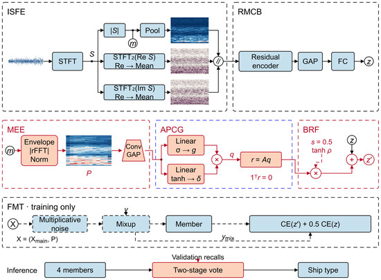
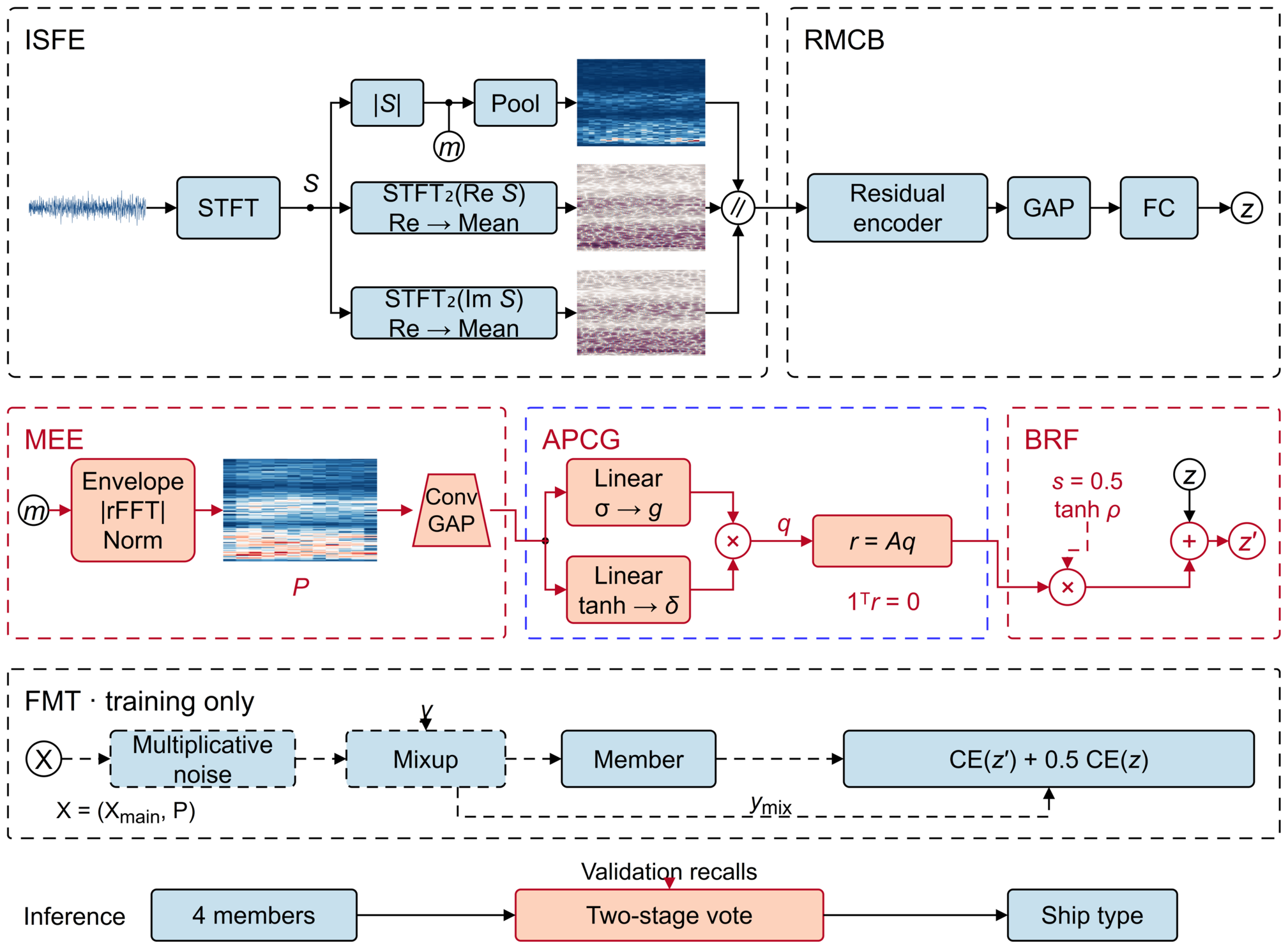
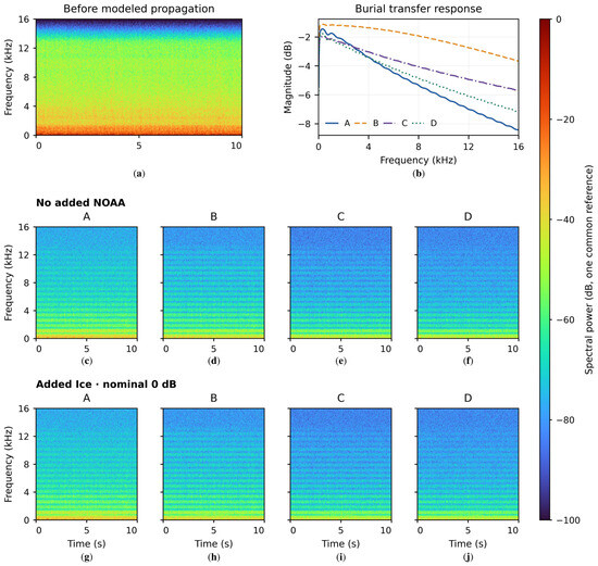
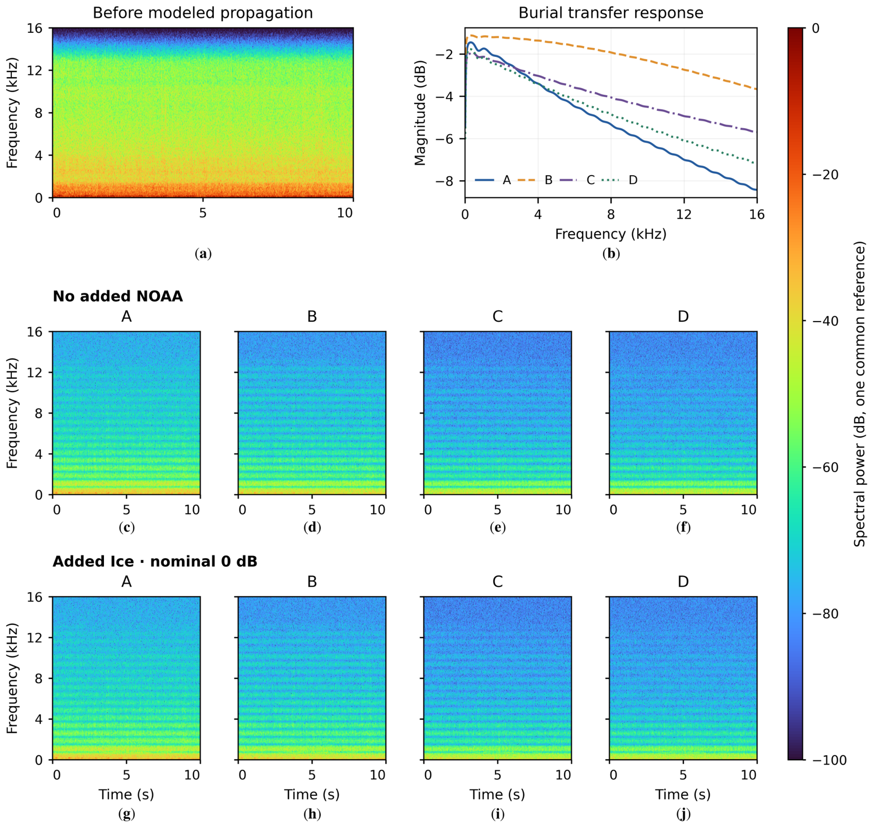
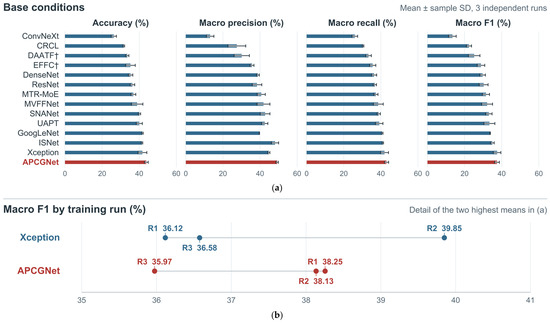
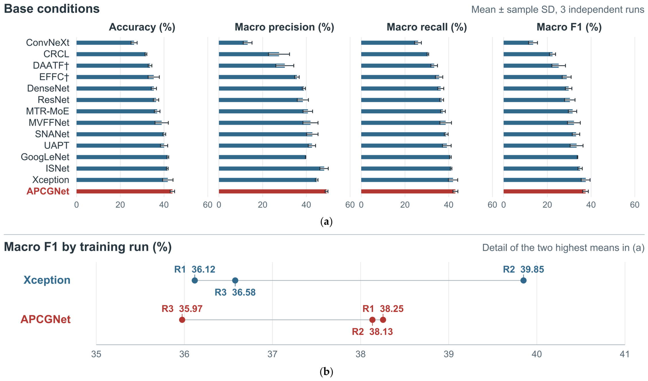
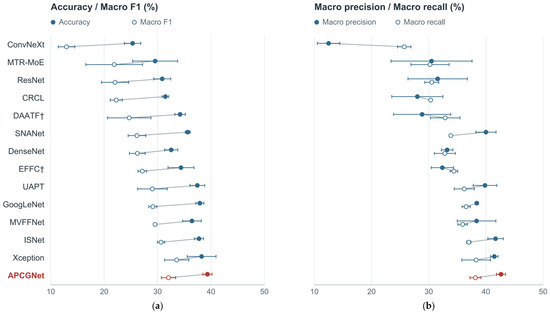
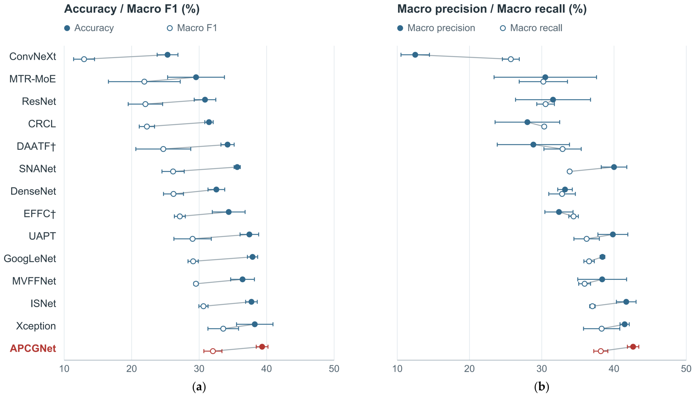
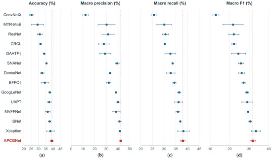
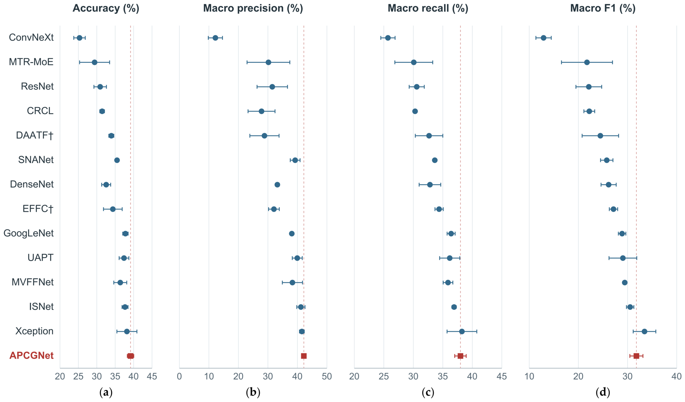
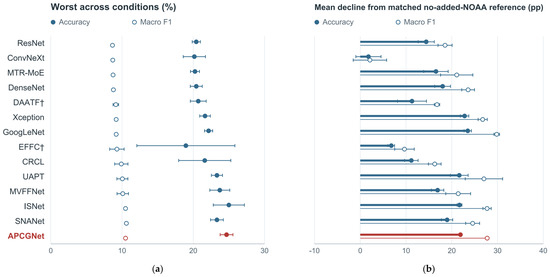
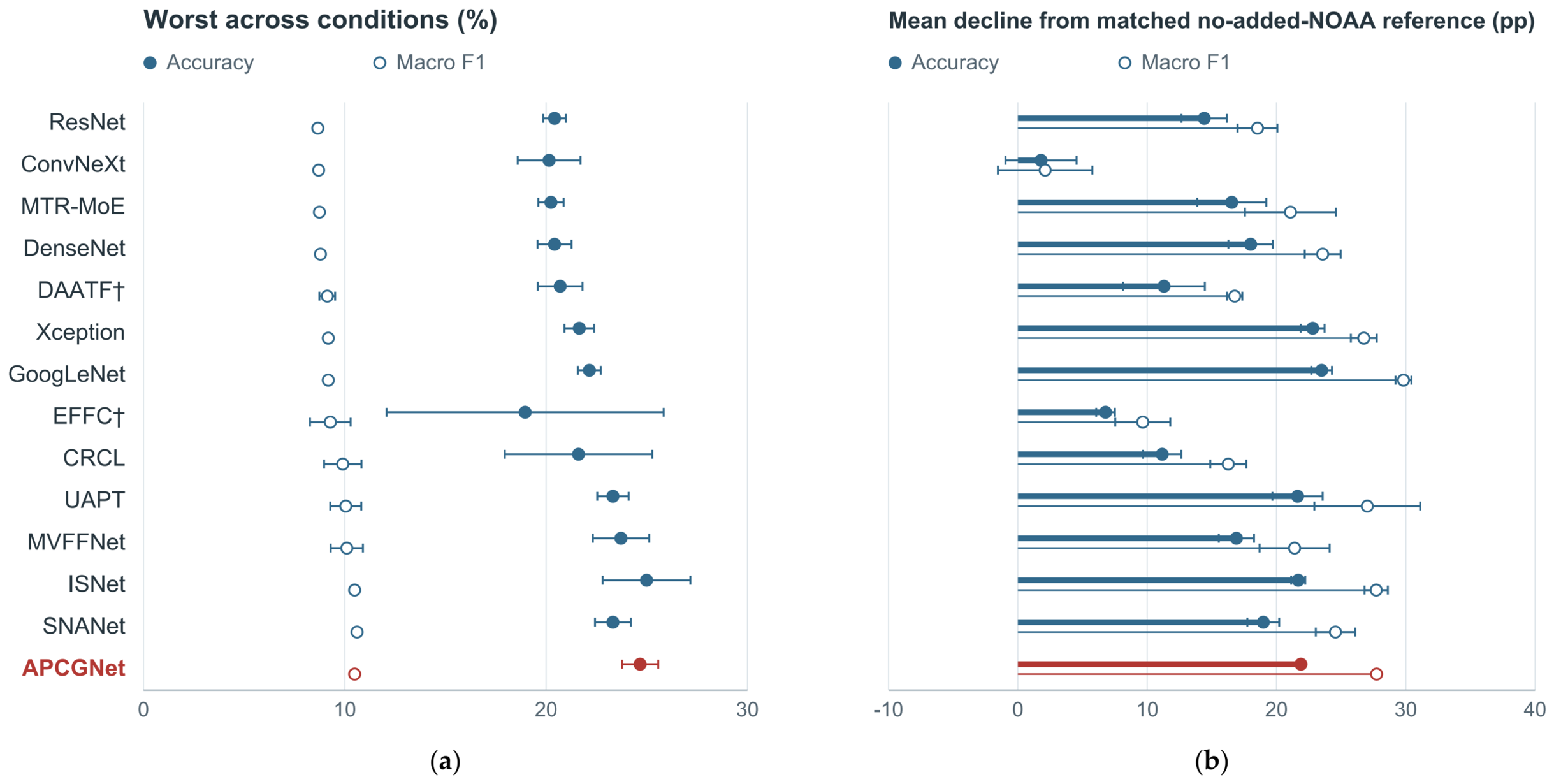
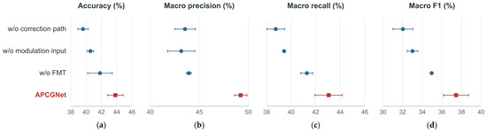
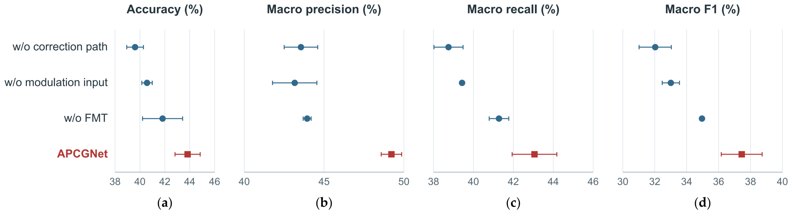
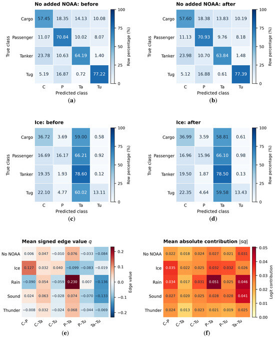
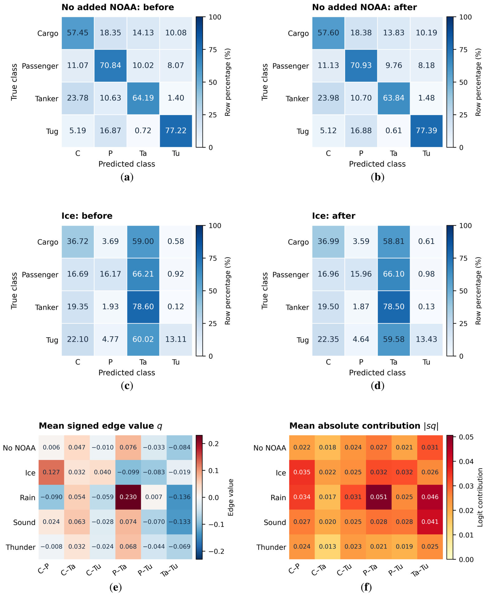

Disclaimer/Publisher’s Note: The statements, opinions and data contained in all publications are solely those of the individual author(s) and contributor(s) and not of MDPI and/or the editor(s). MDPI and/or the editor(s) disclaim responsibility for any injury to people or property resulting from any ideas, methods, instructions or products referred to in the content. |
© 2026 by the authors. Licensee MDPI, Basel, Switzerland. This article is an open access article distributed under the terms and conditions of the Creative Commons Attribution (CC BY) license.