


Abstract
Shortest-distance-path planning cannot satisfy the energy requirements of natural-energy-driven unmanned surface vehicles (NSVs) because it ignores the energy that can be harvested from the environment along the route. This paper develops a global energy-saving path planning method for NSVs by embedding a solar-energy capture weight function into the evaluation functions of the Dijkstra and Theta* algorithms. The grid environment is represented with static obstacles and time-varying cloud occlusion and the improved algorithms bias the search toward nodes with higher solar radiation and lower cloud occlusion so that the planned path avoids obstacles while maximizing the captured energy. The proposed algorithms are compared with the traditional Dijkstra, Theta* and Energy Theta* algorithms, which disregard clouds, under low, medium and high cloud cover; dynamic clouds; and a real marine environment. The improved Theta* algorithm achieves energy balance rates of 91.3%, 91.0% and 84.1% in the low-cloud, dynamic cloud and real marine environment scenarios, respectively, whereas the traditional Theta* algorithm reaches only 50.4% in the real marine environment and the improved Dijkstra algorithm reaches 90.2% and 78.5% in the dynamic cloud and real marine environment scenarios, respectively. These results show that the solar-energy capture weight function raises the captured energy and the energy balance rate, thereby extending the endurance of the NSV.
1. Introduction
USVs [1,2,3,4,5,6,7,8] (unmanned surface vehicles) are efficient offshore intelligent platforms that can be operated remotely or autonomously. They have the advantage of good autonomy, stable working performance, and long navigation time and can perform some dangerous tasks that conventional ships cannot complete. Unmanned boats are usually composed of multiple systems such as power systems, perception systems [9], and control systems [10,11], which can be widely used in military and civilian fields by equipping them with different sensors. With the continuous development of unmanned boat technology, stricter requirements have been put forward in terms of autonomy and endurance. The global path planning method based on the shortest distance is gradually becoming unable to meet these needs. Therefore, this paper proposes an improved Theta* global path planning method considering solar-energy capture to improve the endurance of unmanned boats.
In 2014, T Lolla et al. [12] used MIT’s Multidisciplinary Simulation, Estimation, and Assimilation System (MSEAS) [12] to predict ocean currents in the Philippine Sea and obtained a predictive model for ocean currents in the area. By incorporating the influence of ocean currents into the construction of the level set algorithm evolution function, the time-optimal path planning algorithm is obtained. MSEAS can provide ocean current prediction data at different scales, and T Lolla et al.’s experiments have shown that the scale of ocean current data has a significant impact on the results of time-optimal path planning algorithms.
In 2016, Antonios Tsourdos et al. [13] combined Voronoi diagrams, visual algorithms, and Dijkstra’s search algorithm to propose an improved algorithm for searching energy-saving paths. This algorithm not only searches for a safe, collision-free path but also considers the impact of ocean currents on the energy consumption of USVs. When the state of ocean currents is independent of location, the difference in energy consumption will be minimal. When the state of the ocean current changes greatly with position, the energy consumption difference between the improved path planning algorithm and the visibility–Voronoi shortest algorithm will be significant. The simulation test results show that the proposed algorithm can effectively plan an energy-saving path to ensure the safety of USVs and improve their endurance.
In 2018, Ma Yong et al. [14] proposed an improved PSO algorithm that considers the influence of ocean currents. This algorithm designs an optimization model that considers collision constraints, motion boundaries, and velocity constraints by establishing a motion model for unmanned boats and an energy consumption model of ocean currents on unmanned boats. Fully considering multiple objectives such as sailing distance, path smoothness, safety, and economic cost improved the PSO algorithm. Finally, the effectiveness of the algorithm was verified in simulation experiments in different marine environments.
In 2019, Jia Zhihao et al. [15,16] analyzed the dynamic impact of ocean currents on small, underactuated unmanned boats; established a mathematical model of energy consumption for unmanned boats considering the influence of ocean currents; and designed an energy consumption heuristic function considering the influence of ocean currents based on the principle of the A* algorithm. Through adjustment of the proportion of energy consumption heuristic functions, the energy-saving A* algorithm and energy-saving Simple A algorithm under the action of ocean currents were developed. Finally, the effectiveness of the proposed energy-saving path planning method was demonstrated in simulation experiments.
In 2020, Lu Nibin et al. [17] improved the sparse A* algorithm to address the issue of wave gliders being affected by waves and currents, proposing a path search algorithm that considers static wave and current environments by combining artificial potential field theory to consider navigation safety and design the time-optimal cost function for global path search. On this basis, using the D* algorithm concept, a dynamic path planning search algorithm considering dynamic wave and current environments is proposed. Based on the improved sparse A* algorithm, the original path is not optimal due to changes in the marine environment time during the search process. Then, the algorithm is re-planned at the changing nodes to complete the dynamic global path search. Considering the airworthiness of the planned path, the gradient descent method is used for iteration to obtain a smooth path.
In 2020, Hanlin Niu et al. [18] proposed an energy-saving path planning method for unmanned boats in spatiotemporally changing environments. This method integrates the Voronoi route map method, Dijkstra search algorithm, genetic optimization algorithm, and coastline extension method to address the impact of spatiotemporally changing ocean currents and complex geographic map data on unmanned boat path planning. The paper validated the algorithm using a globally consistent high-resolution coastline dataset and a historical ocean current dataset, demonstrating the practicality and flexibility of the proposed algorithm.
In 2022, Zhipeng Shen et al. [19] proposed an optimization method integrating the improved adaptive ant colony optimization algorithm (RIACO) and the rolling window method (RWM) for the path planning problem of unmanned sailing ships in complex marine environments. This method makes full use of the advantages of the ant colony optimization algorithm in global path search and combines the local dynamic obstacle avoidance ability of the rolling window method at the same time to deal with the challenges brought by sudden obstacles and complex environments. In the research, an obstacle avoidance model suitable for unknown environments was introduced, and the path was smoothed through Bezier curves to enhance the safety and executability of navigation. The simulation experiments show that this method is superior to the traditional methods in both the effect of path planning and real-time performance.
In 2023, Jingrun Liang et al. [20] proposed an optimal path planning method for unmanned surface vessels (USVs) based on the improved White Shark optimizer (IWSO-DWA). In view of the deficiencies of the traditional White Shark optimizer (WSO) in terms of convergence speed, calculation time consumption and dynamic behavior, the author introduced the circular chaotic mapping, adaptive weight factor and simplex methods to improve the quality of the initial solution and search efficiency and combined the optimization results with the Dynamic Window method (DWA) [21,22,23] to improve navigation performance. Meanwhile, the International Maritime Collision Avoidance Code (COLREGs) was incorporated into the route planning to ensure navigation safety. The experimental results show that this method optimizes by 13.66%, 18.78%, 79.08% and 19.85%, respectively, compared with the traditional WSO in terms of path length, turning cost, time consumption and smoothness, and it is capable of achieving efficient, safe and compliant global path planning and real-time obstacle avoidance in complex marine environments.
In 2024, Chaopeng Yang et al. [24,25] proposed an improved path planning algorithm for unmanned surface vehicles (USVs) that combines artificial potential field (APF) with Algorithm A, aiming to address the challenges of maintaining a safe distance and generating efficient paths under the influence of ocean currents. This algorithm improves computational efficiency and obstacle avoidance ability by ignoring unnecessary dangerous nodes, introducing adaptive guiding angles to optimize the search direction, and integrating the potential field force function into the cost function. Finally, the Bezier curve is used to smooth the path. The experimental results show that the new algorithm can effectively plan safe paths under different ocean current conditions, and its average running speed is 22.5% faster than that of the traditional algorithm A.
In 2024, Hang Gao et al. [26] proposed a path planning method for unmanned surface vessels (USVs) based on hybrid maps and the improved Genetic Algorithm (FGA). By combining topological elements and grid maps to construct an efficient environmental model and introducing a feedback mechanism to optimize algorithm performance, experiments show that this method has higher computational efficiency, a shorter path length and smoother continuous paths in complex environments, significantly enhancing the practical application value of USVs.
In addition, for self-guided vehicles operating on land, Mohammadpour et al. [27] developed an energy-efficient local path planning method that considers the load position; comparable energy-aware planning methods exist for ground and legged robots [28,29,30,31,32,33], and such ideas are also relevant to the natural-energy-driven vessel studied in this work.
The Problems of Unmanned Boat Path Technology
Taken together, the existing studies indicate that unmanned boat path planning still has room for improvement, particularly in how environmental factors constrain the planned route and the on-board energy budget; addressing this gap is a prerequisite for transferring the theoretical results into practical ship applications. The main problems with current path planning methods include the following.
(1) Natural-energy capture is not involved
The vast majority of unmanned boats are conventionally powered unmanned boats, and there is no natural-energy capture problem. Even the few natural-energy unmanned boats focus on simple control and planning, so it is necessary to study and explore the natural-energy capture problem involved in path planning.
To clarify the necessity of equipping natural-energy capture devices, even for short-duration construction tasks in offshore scenes, the NSV still relies on the energy captured during navigation to support communication, sensors and propulsion. Without natural-energy supplementation, the vessel has to reserve extra fuel or battery capacity, which increases the mass and reduces the effective load; moreover, for long-endurance missions, the captured energy directly determines the attainable range. Therefore, embedding natural-energy capture into path planning is necessary for both mission reliability and energy economy.
(2) Energy-saving issues in the path are not considered
At present, the vast majority of path planning methods aim to minimize the path and rarely consider the energy-saving issues of unmanned boats. This leads to the consumption of more energy during trajectory tracking, especially for naturally driven unmanned boats, which directly affects their endurance.
(3) Inadequate consideration of constraints
Unmanned boats generally have underactuated characteristics, and most methods do not fully consider the constraints when planning the path, which results in the planned path not meeting the actual needs; this makes it difficult for unmanned boats to track the path and even causes danger. Therefore, it is necessary to consider multiple constraints in the research of unmanned boat path planning and plan a smoother path to ensure the navigation safety of unmanned boats.
The main contributions of this paper are summarized as follows:
(1) A mathematical solar-energy capture model is established, which considers the solar position, cloud occlusion and sea surface reflection, and is verified by the measured photovoltaic data;
(2) An improved global energy-saving path planning framework based on the Dijkstra and Theta* algorithms is proposed, in which the solar-energy capture weight function, the time scheduling for spatiotemporal solar radiation and the line-of-sight accessibility detection are incorporated;
(3) The effectiveness of the proposed algorithms is verified under low/medium/high cloud cover, dynamic cloud environments and a real marine environment, and the improved Theta* algorithm achieves the highest energy balance rate in all cases.
To clarify this study’s novelty with respect to the existing literature, the main technical elements of this work are summarized as follows: (i) The solar-energy capture weight function W(p,t), established from the Berlage scattering model, is analytically coupled with the cost functions of the Dijkstra- and Theta*-based planners (Equations (5), (8) and (10)); to the best of our knowledge, no previous study embeds such an analytical spatiotemporal solar capture weight into graph search path planning. (ii) The line-of-sight (LOS) reachability detection generalizes the standard node direction expansion detection of Theta* to intersection point direction expansion detection, which guarantees that the smoothed path remains trackable under ocean current and underactuation constraints. (iii) The theoretical reason for not designing an explicit energy heuristic term is analyzed in Equations (8) and (9). (iv) The feasibility of extending the proposed planners to bidirectional search is discussed in Section 3.
2. Modeling of Solar Capture for NSV
This section establishes a mathematical model for solar-energy capture that accounts for spatiotemporal variation in solar radiation. Solar position, cloud cover and sea surface reflection are all represented in the model, which provides the basis for computing the solar energy captured by an NSV along any candidate path.
The selected carrier for this article is the “Wave Rider” natural-energy-driven unmanned vessel (NSV) [34]. The experiments were provided only as background illustration. Currently, two generations have been developed, as shown in Figure 1. The deck of the “Wave Rider II” is equipped with four sets of solar panels, each with a peak power of 630 W. It is also equipped with a three-bladed wind turbine with a peak power of 600 W. In addition, it carries high-performance lithium batteries to store the electricity generated by the solar panels and wind turbines, providing power for onboard electrical appliances. The propulsion mode of this unmanned boat is a hybrid drive mode of single propeller and single rudder and wave-energy drive. At the same time, the four pairs of hydrofoils installed at the front of the hull can convert the wave-induced heave and pitch motion of the hull into forward thrust. The NSV of the “Wave Rider II” achieves the complementarity of wind, light, and waves and has high endurance. Currently, the accumulated test range exceeds 3000 km.
Figure 1.
NSV. The Chinese characters on the hull are the vessel’s name, “Yu Lang Zhe” (Wave Rider).
According to the resistance model of Ref. [35], the energy-saving speed can be obtained as:
2.1. Mathematical Model for Solar-Energy Capture
Intensity of Scattered Solar Radiation
Based on the observed solar radiation in the sky, the calculation formula for scattered radiation intensity can be derived using the Berlage formula [36] as follows:
where is the solar altitude angle, and the unit is °; is the relative atmospheric air mass (dimensionless), i.e., the ratio of the slant optical path of solar radiation through the atmosphere to the zenith optical path; is the atmospheric transparency coefficient (dimensionless, in the range of 0–1), representing the fraction of solar radiation transmitted through one unit of air mass; is the intensity of solar radiation; and is the intensity of solar radiation on the horizontal plane.
2.2. Verification of Mathematical Model for Solar-Energy Capture [2]
To verify the established mathematical model for solar-energy capture and the measurement of low, medium, and high cloud cover solar radiation, the latitude and longitude coordinates of the Ship Sea Building at Harbin Engineering University are 126.681 degrees east longitude and 45.777 degrees north latitude. We carried out photovoltaic measurement experiments on the rooftop of the building.
We calculated the hourly solar radiation intensity and daily average solar radiation and then compared them with the actual statistical data measured at the sampling site to verify the accuracy of the established mathematical model.
The key environmental parameters of the experimental scheme are summarized as follows: the experiment was conducted on the rooftop of the Ship Sea Building of Harbin Engineering University (126.681° E, 45.777° N); a total solar radiation sensor was installed on a horizontal plane free of artificial shading (Figure 2a,b); and the hourly and daily average solar radiation were recorded for comparison with the statistical data of the local meteorological station. The photovoltaic parameters used in the experiment were consistent with the flat-laying configuration of the NSV under study: four solar panels with a peak power of 630 W each, a total panel area of 10 m2, and a conversion efficiency of 15%. The measurement covered clear-sky, partially cloudy and overcast winter conditions so that the low, medium and high cloud cover scenarios could be evaluated, as shown in Table 1 and Table 2.
Figure 2.
Solar-Energy Experiment Diagram.
Table 1.
Hourly solar radiation intensity in Harbin in November (W/m2).
Table 2.
Comparison of daily hourly solar radiation intensity on the horizontal plane in Harbin in November (W/m2).
The “Winter Solar Radiation Illumination Table of Major Cities in China” provides relevant data on winter solar radiation in eight cities, including Beijing and Harbin. To keep the comparison authentic, Harbin is selected as the sampling location for calculation and comparison. The solar radiation intensity in Harbin in November is shown in Table 1.
Figure 3 plots the photovoltaic power generation test data.
Figure 3.
Photovoltaic power generation test data.
Harbin is located at latitude 44°4′–46°40′ N and longitude 125°42′–130°10′ E. For the calculation method, the sampling geographic latitude was taken as 45° N, and the sampling time was on 26 November, with a sampling day sequence of 330 days. During the calculation, both direct and scattered solar radiation were considered, and reflected radiation was ignored. The calculated results are shown in Table 2.
Because the laying method of the solar panels for the NSV studied in this article is flat, the accuracy of calculating the solar radiation intensity on the horizontal plane is relatively high. From Table 2, it can be seen that the calculated daily total radiation has an error of approximately 1% compared to the statistical results. Therefore, it is considered that the mathematical model is in line with the actual situation and can be used for simulation experiments. Berlage formula [36] can be used to calculate the solar-energy capture of the experiment.
With regard to the sea state condition, which is an important factor for the solar-energy capture of a USV operating in real marine environments, the rooftop experiment at Harbin Engineering University is used to verify the accuracy of the solar radiation model on a horizontal plane, and the sea state influence is incorporated in this study through two mechanisms. First, the sea surface reflection term of the solar radiation model (Section 2.1) accounts for the effect of the sea surface on the incident radiation. Second, the simulations in Section 4.3 are carried out in a real marine environment (the South China Sea) using realistic wind, wave and current data, which indirectly reflects the effect of the sea state on the energy consumption side. The remaining influence of wave-induced panel inclination on the effective solar incidence angle is assumed to be negligible for the low-to-moderate sea states considered here and will be quantified in the planned sea trials of the “Wave Rider II” platform, as stated in Section 5.
2.3. Design of Weight Function Based on Solar-Energy Capture
The intensity of solar radiation will change over time, so when designing the weight function, it is necessary to consider the local time when the NSV is moving. At the same time, due to the shielding effect of the upper structure of the NSV on the solar panel, it is also necessary to consider the impact of different angles of incidence of solar rays on the light harvesting area.
Firstly, we analyze the shielding effect of the NSV superstructure. Given the known solar altitude and azimuth, it is necessary to compare the maximum horizontal horizon angle of the solar panel with the solar altitude angle. If it is greater than the solar altitude angle, it is within the shadow range and the solar radiation intensity is zero; Otherwise, radiation intensity reduction calculation is required. However, due to the fact that the main component of the upper structure of NSV is the bracket for installing sensors, in practical situations, even if the maximum horizontal horizon angle of the solar panel is greater than the solar elevation angle, the solar radiation intensity will not be zero. Therefore, the shading area of the solar panel is calculated as follows:
where indicates the intensity of direct solar radiation and indicates the intensity of solar scattered radiation.
From the above equation, it can be seen that the solar energy captured by NSV solar panels per unit time is only related to the navigation time. Therefore, the weight function for solar-energy capture can be designed as follows:
where E_sun(j) indicates the amount of solar energy captured from the starting point to the point j; E_sun(k) represents the amount of solar energy captured from the starting point to the point k; and E_sun(k, j) represents the amount of solar energy captured from point k to point j.
Substitute the above weight functions into the Dijkstra and Theta* algorithms to obtain an improved Dijkstra and Theta* global path planning algorithm based on solar-energy capture.
3. Natural-Energy Optimization Path Planning Method
3.1. Energy Optimization Improvement Strategy Based on Dijkstra Algorithm [37]
In Dijkstra’s algorithm, the position where the starting point is located is called the initial node. The evaluation function of Dijkstra’s algorithm is:
In the formula, is the actual consumption from the initial node to any node on the map, usually calculated as the actual distance from the starting point to the current node.
The Energy Theta* algorithm assumes a static environment, in which the obstacle positions do not change over time or space. The search then needs to account only for the spatial layout of obstacles, and time can be left out of the node evaluation. Meteorological conditions, by contrast, vary strongly in both space and time and cannot be neglected. The improved Dijkstra algorithm therefore incorporates the time dimension as well. To record the temporal evolution during the search, each node stores a schedule, denoted as .
The complete process of the improved Dijkstra algorithm is as follows:
- (1)
- Place the starting point in the OPEN collection and set it as the current node . Record the starting point and departure time as ; simultaneously set the evaluation value to 0.
- (2)
- If the OPEN set is empty, the search will fail and the algorithm will stop.
- (3)
- Calculate the minimum evaluation value of a node in the OPEN set, place the node in the CLOSED set, set it as the current node , and store the time from the starting point to the current node in the schedule .
- (4)
- Determine whether the node is the target point. If so, end the loop and skip to Step (9).
- (5)
- Adjacent nodes of the access node (up, down, left, right, top left, bottom left, top right, and bottom right directions) are subjected to node direction expansion detection for each of the above 8 directions. If a node direction is not expandable, delete that node direction and save other node directions as passed in Step (6). The corresponding neighboring nodes are called the child nodes of the current node. The current node is the parent node of all expansion direction nodes. The direction of the child node always points to the parent node.
- (6)
- Extract and calculate environmental data through an environmental data model based on the time information in the schedule . Substitute the corresponding environmental data and node direction (heading information) into the evaluation function to calculate the evaluation value .
- (7)
- Determine the visited child nodes, and if the neighboring nodes are in the CLOSED set or the child nodes are obstacle nodes, proceed to Step (2).
- (8)
- Determine whether the child node is in the OPEN set. If not, add it to the OPEN set; if so, update the evaluation values of the child nodes and the parent node and update the time information in the child node schedule , then proceed to Step (2).
- (9)
- Trace back the nodes in the CLOSED set, generate paths based on the pointing of child nodes and calculate the total energy consumption of the paths.
The flowchart of the improved Dijkstra algorithm is shown in Figure 4.
Figure 4.
Improved Dijkstra Algorithm Flow Chart.
The Energy Theta* algorithm can improve its search efficiency by adding heuristic terms to the evaluation function. The improved mathematical formula is:
In the formula, represents the estimated cost from the current point to the target point, usually calculated using Euclidean distance or Manhattan distance. The improved algorithm is called A*. If the A* algorithm wants to find the optimal path, it has requirements for the heuristic term in the evaluation function, and the mathematical expression required is:
In the formula, represents the actual cost from the current node to the target node. The following discusses why not to add heuristic terms to improve the search efficiency of Dijkstra’s algorithm.
The evaluation function of the traditional A* algorithm is usually distance. Whether the Euclidean distance or the Manhattan distance is used, the actual distance between two nodes is always greater than or equal to the heuristic distance, which is also the key to A* algorithm finding the optimal value. However, in improving the Dijkstra algorithm, in order to match , the heuristic term should be set as the estimated energy consumption value of NSV from the current node to the target node. Due to the influence of spatial and temporal changes in the marine environment, it is impossible to determine which inputs of environmental information should be used with the Manhattan distance; if the Euclidean distance is used, it can be seen that although straight-line distance is the shortest distance, it does not mean that the net energy consumption after considering energy capture and energy consumption is the lowest. Because it cannot be guaranteed that the estimated energy consumption of the NSV from the current node to the target node is not greater than the actual consumption, it cannot be guaranteed that the path optimization algorithm will not improve the Dijkstra algorithm by improving the energy heuristic term if it finds the optimal value.
3.2. Energy Optimization Path Planning Method Based on Theta* Algorithm
3.2.1. The Basic Principle of Theta* Algorithm [38]
The improved Dijkstra algorithm is derived from the Dijkstra algorithm, and due to the limitations of the grid and search direction, there are 8 possible directions for the path with intervals of 45 ° between 0 and 360 °. Strictly speaking, this path is not the shortest path in continuous space, as shown in Figure 5.
Figure 5.
Shortest Path in Continuous Space.
Figure 5a is planned using Dijkstra’s algorithm, and the shortest path from Point A4 to Point C1 consists of 4 nodes. However, in reality, the shortest path should be the straight path in Figure 5b, which only requires 3 nodes. To address this issue, Hart et al. [39] proposed the A* algorithm in 1968, and Thorpe and Matthies [40] extended it with post-smoothing in 1984. The algorithm first uses the A* algorithm to search and calculate the optimal path and then smooths and processes the path. The key step in this process is gaze detection. As the name suggests, line-of-sight detection involves imagining a person looking at another point from one point. If there are no obstacles blocking the path between the two points, they can directly see the other point through their line of sight, which is called line-of-sight detection passing. Otherwise, it does not pass.
The smoothing post-processing process actually starts from the starting point and checks whether the next node of the current node on the path is connected to the parent node of the current node with a collision-free straight line. If such a collision-free straight line exists, the parent node of the current node is taken as the parent node of the next node, and the current node is deleted from the path point until the target point is reached. Using pre-planned paths for post-processing can result in shorter paths than the original method, but there is still a possibility of getting stuck in local minima. As shown in Figure 6, the blue dashed line represents the shortest path calculated by Dijkstra’s algorithm; the blue solid line represents the shortest path after post-smoothing, but in reality, the true shortest path is the red dashed line. Because the blue solid line of post-processing is constrained by the initially calculated nodes and cannot achieve the effect of the red dashed path, the post-processing method cannot guarantee the optimal result of the path. This requires the algorithm to perform smoothing during the search process. To achieve this goal, Daniel [38] developed the Theta* algorithm in 2010.
Figure 6.
Comparison of Different Paths. The blue squares denote the obstacle grid cells.
The biggest difference between the Theta* algorithm [41] and Dijkstra’s algorithm is that during the search process, not only do we need to compare the size of node extensions, but we also need to consider whether there are redundant nodes in the path, which requires line-of-sight detection. Nodes detected through the line of sight need to be deleted and handed over to their parent nodes. This process is called the node update process.
3.2.2. Optimal Energy Improvement Strategy Based on Theta* Algorithm
Like the improved Dijkstra algorithm, the Theta* Energy Path Planning method based on the Theta* algorithm also requires node direction expansion detection during path search. The detection method is consistent with the improved Dijkstra algorithm, using the ground speed to solve the NSV. If the speed is equal to 0 or there is no solution, this indicates that the expansion direction should be deleted.
In the LOS detection, the ground velocity of the NSV is obtained from the velocity triangle V_ground = V_water + V_current, where V_water is the water-referenced speed determined by the energy-saving speed profile described in Section 4 and V_current is the ocean current vector stored in the environmental grid map. An expansion direction is deleted when (i) the computed ground speed is zero or (ii) the velocity triangle has no real solution (i.e., the current magnitude exceeds the maximum achievable water speed of the NSV in that direction); otherwise, the direction is retained. The current field used in the simulations is provided by the environmental grid map described in Section 4.1.
The biggest feature of the Theta* algorithm compared to Dijkstra’s algorithm is its line-of-sight detection during the search process. Improving the Theta* algorithm also adds this step, but due to the actual navigation performance of the NSV and the influence of marine environmental factors, the new path detected by line of sight may not be able to complete the route tracking task. Therefore, it is necessary to add a line-of-sight reachability detection process to the new path. Only the path detected by this detection process can become a true candidate path for evaluation and estimation. In layman’s terms, in improving the Theta* algorithm, the reason for the inability to expand the line of sight is not only due to obstruction from obstacles but also due to factors such as excessive ocean currents, which prevent the NSV from navigating along this route.
The process of line-of-sight accessibility detection requires knowledge of node direction extension detection. In other words, this process is similar to a combination of multiple node direction extension detection, but it is not the actual detection of nodes but rather the detection of intersection points. As shown in Figure 7, the two nodes of this path cross many grids, and there are multiple intersection points between the path and the grid boundaries. Due to the different marine environment information of each grid, it is necessary to perform intersection direction expansion detection for each section of the path. If any section of the detection fails, it means that the line-of-sight accessibility detection fails.
Figure 7.
Schematic diagram of line-of-sight accessibility detection.
The process of visual accessibility detection involves the following two issues: firstly, the calculation of intersection coordinates, and secondly, the detection of intersection direction expansion. The process of obtaining intersection coordinates is as follows:
(1) Find two nodes and along a straight path in grid space. Assign the horizontal axis to and the vertical axis to , assign the horizontal axis to and the vertical axis to , assign the change in the vertical axis to , and assign the change in the horizontal axis to .
(2) If and , proceed to Step (3); if and , proceed to Step (4); if and , proceed to Step (5).
(3) Determine the number of intersection points that include the starting and ending endpoints and create a sequence of intersection points . The horizontal axis is equal to , and the vertical axis is equal to ; the horizontal axis is equal to, and the vertical axis is equal to . The horizontal axis is equal to and , the vertical axis is equal to, and the corresponding element in the arithmetic sequence is with an interval of.
(4) Determine the number of intersection points that include the starting and ending endpoints and create a sequence of intersection points . The horizontal axis is equal to , and the vertical axis is equal to ; the horizontal axis is equal to , and the vertical axis is equal to . The vertical axis is equal to , the horizontal axis is equal to , and the corresponding element in the arithmetic sequence is with an interval of.
(5) Assign all grid horizontal coordinates between and to calculate all intersection points between line segments and straight lines; assign all grid coordinates between and to calculate all intersection points between line segments and straight lines; combine all the intersection points obtained above to obtain a sequence of intersection points, and arrange them in ascending order on the x-axis.
(6) If is greater than 0, then the intersection coordinates are in the sequence of positive sequence intersection points; otherwise, the intersection coordinates are in reverse order of the intersection sequence .
The intersection sequence includes the two endpoints of the line to be detected, and its direction extension detection follows the same rules as node direction extension detection. The overall detection procedure can then be summarized as follows:
(1) Calculate the sequence of intersection points using the method of obtaining intersection point coordinates, and let , , .
(2) Perform intersection direction expansion detection on nodes and ; if passed, , ; if it fails, the line-of-sight accessibility detection fails and the algorithm ends.
(3) If is greater than , end the algorithm and pass the line-of-sight accessibility detection; otherwise, return to Step (2).
The evaluation function of the improved Theta* algorithm is similar to that of the improved Dijkstra algorithm. When the route is the second type mentioned above, its evaluation value is calculated using Equation (8); when the route is the first type mentioned above, its evaluation value is calculated using Equation (8):
In the formula, there are k + 1 intersection points in the first route, including the two endpoints of the path; that is, there are k sub-path segments. P_j is the propulsion power of the j-th sub-path segment; d_j is the distance of the j-th sub-path segment, which can be calculated according to Formula (9); and v_j is the navigation speed of the j-th sub-path segment.
In the formula, i represents the current intersection point; j represents the next intersection point in the direction of the route; lat_i and lon_i represent the latitude and longitude of the current intersection point, respectively; lat_j and lon_j represent the latitude and longitude of the next intersection point, respectively; and R_e is the Earth’s radius.
The search efficiency of the Theta* algorithm can also be improved by setting appropriate heuristic terms in the evaluation function. The setting of heuristic terms should be consistent with the A* algorithm, as shown in Equation (9). However, due to the fact that the evaluation function of the improved Theta* algorithm calculates energy rather than distance, there is a problem that it is difficult to calculate the actual energy, so an energy heuristic term is not designed.
Bidirectional search is an optimization method that reduces the computational load of path planning by simultaneously expanding the search tree from both the starting point and the ending point. In global path planning, the core idea is bidirectional parallel expansion. When the search trees at both ends meet at the middle node, the path search terminates, thereby significantly reducing the number of node expansions and computational complexity. The applicable scenarios of two-way search are suitable for situations where the map area is large and the distribution of obstacles is sparse. Combining solar capture, obstacle avoidance, and dynamic constraints (such as underactuation characteristics), bidirectional search can quickly find feasible paths under complex constraints.
Bidirectional parallel expansion is not implemented in the current pseudo-codes, and the qualitative comparison in Table 3 is intended as a reference for future extensions rather than a claim about the implemented algorithms.
Table 3.
Qualitative comparison between one-way search and bidirectional search. Note that Algorithms 1 and 2 implement one-way (single-direction) search: the search tree is expanded from the start node S toward the target node T only.
| Algorithm 1: Improved Dijkstra with solar-aware cost function |
| Input: grid map G, start S, goal T, solar capture weight W(p,t), trade-off parameter alpha Output: path P 1: OPEN <- {S}, CLOSED <- empty, g(S) <- 0, parent(S) <- null 2: while OPEN is not empty do 3: n <- node in OPEN with minimum f(n) = g(n) − alpha*E_solar(n) 4: move n from OPEN to CLOSED 5: if n = T, then break 6: for each 8-connected neighbor m of n do 7: if m is an obstacle, then continue 8: if direction expansion detection (ground-speed check) fails for n -> m, then continue 9: tentative <- g(n) + dist(n,m)*epsilon(V*) + env_cost(n -> m) 10: if tentative < g(m), then 11: g(m) <- tentative, parent(m) <- n, update E_solar(m) 12: update f(m) = g(m) − alpha*E_solar(m) 13: if m not in OPEN, then add m to OPEN 14: return path by tracing parents from T to S |
| Algorithm 2: Improved Theta* with solar-aware cost and LOS reachability |
| Input: grid map G, start S, goal T, solar capture weight W(p,t), trade-off parameter alpha Output: path P 1: OPEN <- {S}, CLOSED <- empty, g(S) <- 0, parent(S) <- S 2: while OPEN is not empty, do 3: n <- node in OPEN with minimum f(n) = g(n) − alpha*E_solar(n) 4: move n from OPEN to CLOSED 5: if n = T then break 6: for each 8-connected neighbor m of n, do 7: if line of sight exists between parent(n) and m and LOS-reachability detection passes, then 8: if g(parent(n)) + dist(parent(n),m)*epsilon(V*) + env_cost < g(m), then 9: g(m) <- g(parent(n)) + dist(parent(n),m)*epsilon(V*) + env_cost 10: parent(m) <- parent(n), update E_solar(m) 11: otherwise, if direction expansion detection passes for n -> m, then 12: if g(n) + dist(n,m)*epsilon(V*) + env_cost < g(m), then 13: g(m) <- g(n) + dist(n,m)*epsilon(V*) + env_cost, parent(m) <- n 14: update f(m) 15: return path by tracing parents from T to S |
Heuristic guidance for bidirectional search: Design symmetrical heuristic functions (such as bidirectional A*) to guide the search trees at both ends to approach each other rapidly. Dynamically adjust search weights: Dynamically adjust the expansion priority of the starting tree and the ending tree based on environmental complexity (such as cloud density and obstacle distribution).
Figure 8 and Figure 9 visually compare the planned paths before and after optimization, respectively: after introducing the solar-energy capture function, the planned path no longer only pursues the shortest distance but also actively passes through areas with higher solar radiation, which is the direct reason why the improved algorithm achieves a higher energy balance rate without obvious sacrifice of path length.
Figure 8.
Before optimization.
Figure 9.
After optimization.
The path cost function takes into account solar capture:
The path cost function of the improved Theta* algorithm not only considers the distance of the path but also introduces the solar capture amount as a weight. The formula is as follows:
where is the actual path cost from the starting point to the node (such as distance or energy consumption), is heuristic cost estimation from the node to the target point (such as Euclidean distance), is solar energy captured at the node , and is trade-off parameters used to adjust the weight of solar capture in path planning.
In Equation (10), the actual path cost g(n), the heuristic term h(n) and the solar capture reward E_solar(n) are all expressed in the same energy unit (MJ), so they can be directly added or subtracted without additional normalization; the solar capture reward enters the cost function with a negative sign through the trade-off parameter. The trade-off parameter alpha is dimensionless, in the range [0, 2] and is calibrated by a grid search on the training simulations; the calibrated values under different seasons and weather conditions are listed in Table 4 and Table 5.
Table 4.
The trade-off parameters are illustrated based on the seasonal variation values.
Table 5.
The trade-off parameters are illustrated based on the weather change values table.
In the actual implementation of Algorithms 1 and 2, the heuristic term h(n) is set to zero (h(n) ≡ 0) because the solar-aware cost is already embedded in the node cost and the search grid is uniformly sampled; the evaluation function used in the pseudo-codes therefore reduces to f(n) = g(n) − alpha×E_solar(n), which is consistent with Equation (10) when h(n) = 0. With this simplification, Equation (10) and the pseudo-codes of Algorithms 1 and 2 are equivalent.
Trade-off parameters control the weight of solar capture in the path cost function. They set the relative importance of solar capture against energy consumption: a larger gives solar capture more weight, so the search tends to prefer paths that collect more solar energy even when they are somewhat longer or consume more propulsion energy. A smaller value makes the direct energy consumption (determined by and ) dominant, and the planner leans toward the shortest or least-consuming path at the expense of solar gain. The parameter can also be adapted to the operating environment: when solar resources are abundant (e.g., on sunny days), can be raised to make fuller use of solar energy and reduce the draw on stored energy; when solar resources are scarce (e.g., cloudy days or at night), can be lowered so that the planner focuses on the direct energy consumption of the path.
The range of values usually depends on the scenario and the requirements of the problem. The weight must stay positive, because the captured solar energy reduces the overall path cost; a negative or zero weight would discard this benefit. The specific value is set by experiment or prior experience and is usually tuned according to the relative importance of energy consumption and solar capture in the target scenario; adjustments are therefore application-dependent rather than fixed.
The trade-off parameter lets the planner strike a balance between energy consumption and solar capture. A suitable value improves both the energy efficiency of the planned route and the practicality of the result, allowing an unmanned vessel to make better use of solar energy at sea and to extend its endurance.
As with the improved Dijkstra algorithm, the improved Theta* algorithm must also account for the time dimension. To keep track of the temporal evolution during the search, a schedule is stored for each node, denoted as . The complete procedure is described as follows:
(1) Initialize the starting point and target point. Place the starting point in the OPEN collection and set it as the current node . Record the starting point and departure time as ; simultaneously set the evaluation value to 0.
(2) If the OPEN set is empty, the search will fail and the algorithm will stop.
(3) Calculate the minimum evaluation value of a node in the OPEN set, place the node in the CLOSED set, set it as the current node , and store the time from the starting point to the current node in the schedule .
(4) Determine whether the node is the target point. If so, end the loop and skip to Step (8).
(5) Visit neighboring nodes of the access node and determine whether they are obstacles or already in the CLOSED set. If so, proceed to Step (7). If not, proceed to Step (6).
(6) Perform the energy node update process:
a. Take the current node and its neighboring nodes as processing objects.
b. Perform line-of-sight detection and line-of-sight reachability detection on the parent node and neighboring nodes of the current node . If it passes, proceed to Step c. If it does not pass, proceed to Step e.
c. Determine whether the sum of the consumption from the starting point to the parent node plus the consumption from the parent node’s straight line to the neighboring node is less than the consumption of the original path from the starting point to the neighboring node , update the consumption value of the neighboring node and set the parent node of the neighboring node to p(n); simultaneously update the time from the starting point to neighboring nodes and record it in the schedule .
d. Determine if is in the OPEN set; will be removed.
e. Determine whether the sum of the consumption from the starting point to the current node plus the consumption from the current node to neighboring nodes is less than the consumption of the original path from the starting point to neighboring nodes , update the consumption value of neighboring nodes and set the parent node of the neighboring node to ; simultaneously update the time from the starting point to neighboring nodes and record it in the schedule .
f. Determine if is in the OPEN set; will be removed.
(7) Add the node to the CLOSED collection and proceed to Step (2).
(8) Trace back the nodes in the CLOSED set, generate paths based on the pointing of child nodes and calculate the total energy consumption of the paths in .
Figure 10 presents the flowchart of the Theta* algorithm.
Figure 10.
Theta* Algorithm Flow Chart.
To quantitatively evaluate the net solar-energy benefit of a planned route, the energy balance rate (EBR) is formally defined as the ratio of the surplus energy to the captured energy:
where E_captured is the total solar energy captured by the solar panels along the route and E_consumed is the total energy consumed by the NSV during navigation; the surplus energy E_surplus = E_captured − E_consumed is reported in Table 6, Table 7, Table 8, Table 9 and Table 10.
Table 6.
Comparison of simulation results under low cloud cover.
Table 7.
Comparison of simulation results under medium cloud cover.
Table 8.
Comparison of simulation results under high cloud cover.
Table 9.
Comparison of simulation results in dynamic environment.
Table 10.
Comparison of simulation results in real environments.
4. Algorithm Simulation Experiment Research
This section compares the proposed algorithms with the baseline variants under identical operating conditions: the improved Dijkstra and improved Theta* algorithms that embed solar-energy capture are tested against the Energy Theta* and traditional Theta* algorithms. Cloud interference is included in the improved Theta* search, while the Energy Theta* variant neglects it.
4.1. Static Simulation Under Cloud Cover
According to Ref. [35], the calculated light intensity is 157.87 W/m2, the solar panel area is 10 m2, and the energy conversion rate of the solar panel used by NSV is 15%.
The control variables that need to be set in the simulation environment mainly include the resolution of the map model being 92 × 60. To make the simulation more realistic, real coastline geographic coordinates are used to represent the areas of longitude 107° E–130° E and latitude 8° N–23° N in the South China Sea and surrounding waters. The starting point position is 17° N–113° E, and the ending point position is 17° N–125° E. The black part in the figure represents obstacles, and the gray part represents clouds. The darker the gray level, the thicker the clouds, that is, the lower the transmittance. The simulation experiment platform is Python 3.7, and the hardware platform’s processor is Intel Core i3-8100, with a clock speed of 3.6 GHz and 8 GB of running memory.
4.1.1. Energy System Parameters Used in the Simulations
The energy model used in the simulations is specified as follows, based on the Wave Rider II platform design [34] and the resistance model of Ref. [35]. The propulsion power is computed as P_prop = R(V) × V/eta_p, where R(V) is the total resistance at speed V obtained from the resistance model [35] and eta_p = 0.55 is the combined propulsion efficiency of the propeller, shaft and motor. A constant onboard electrical load P_load = 30 W (communication, navigation, sensors and controller) is added to the propulsion power. The power converter (MPPT and DC/DC) has an efficiency of eta_conv = 0.92, and the battery (10 kWh LiFePO4) has a charge/discharge efficiency of 0.95. The state of charge (SOC) is maintained within [0.2, 0.95], with an initial SOC of 0.9 and a protection threshold SOC of 0.2; when the SOC approaches the threshold, the energy consumption weight in the path cost function is increased so as to avoid over-discharge. The energy consumption of a route segment is accumulated as (P_prop + P_load)/eta_conv multiplied by the navigation time of the segment, and the unit-distance propulsion energy is evaluated at the energy-optimal cruise speed V* = 0.755 m/s.
V* = 0.755 m/s is the energy-optimal cruise speed derived from the resistance model [35]; it is used only to compute the unit-distance propulsion energy consumption. The task duration reported in Table 6, Table 7, Table 8, Table 9 and Table 10 is the total navigation time of the entire planned route, which includes steering, detours caused by obstacles and clouds, and the lower effective speed under real wave and current conditions. Therefore, the average speed of a 1410 km route completed in 1763 h is about 0.22 m/s, which is not contradictory to the cruise speed V* used in the energy model.
4.1.2. Implementation Details for Reproducibility
For reproducibility, the following implementation details are provided. Map: The simulation area is 107° E–130° E in longitude and 8° N–23° N in latitude, discretized into a 92 × 60 grid with a grid size of 0.25 degrees; the start point is (17° N, 113° E), and the goal point is (17 N°, 125 E°). Obstacles: Land and islands are encoded as static obstacles using real coastline geographic coordinates. Cloud cover model: The cloud transmittance is represented by a grayscale grid [42] generated from the ERA5-derived cloud cover data, in which darker cells correspond to thicker clouds and lower transmittance; the transmittance is combined with the Berlage scattering model to obtain the incident radiation on the solar panels. Environment-update rule: The solar radiation intensity is updated every simulation hour according to the solar position, and in the dynamic cloud scenario, the cloud transmittance grid is updated every 30 min according to a prescribed cloud motion model. Solar panels: There are four panels with a peak power of 630 W each, a total area of 10 m2 and a conversion efficiency of 15% [34]. Battery: The battery is a 10 kWh LiFePO4, with the SOC range and efficiencies given in Section 4.1.1. The pseudo-codes of the two proposed algorithms are given below.
Here, dist(n,m) denotes the great-circle distance between nodes n and m computed by Equation (9), epsilon(V*) denotes the unit energy consumption coefficient per kilometer evaluated at the energy-saving speed profile V* described in Section 4, and env_cost denotes the environment-dependent correction accumulated along the considered edge (e.g., the extra resistance caused by the ocean current), which is read from the environmental grid map. These quantities are used in Algorithm 2 only to compare candidate edges, and they are expressed in the same units as g(n).
(1) Simulation comparison under low cloud cover
Figure 11, Figure 12, Figure 13 and Figure 14 show the low cloud cover results of the four algorithms: the route of the Energy Theta* algorithm in Figure 11, that of the improved Dijkstra algorithm with solar capture in Figure 12, that of the traditional Theta* algorithm in Figure 13, and that of the improved Theta* algorithm with solar capture in Figure 14. In each panel, the green marker on the left is the start point, the red marker on the right is the target point, and the green line between them is the planned route.
Figure 11.
Energy Theta* algorithm. The green marker on the left is the start point, the red marker on the right is the target point, and the green line is the planned route.
Figure 12.
Improved Dijkstra algorithm. The green marker on the left is the start point, the red marker on the right is the target point, and the green line is the planned route.
Figure 13.
Traditional Theta* algorithm. The green marker on the left is the start point, the red marker on the right is the target point, and the green line is the planned route.
Figure 14.
Improved Theta* algorithm. The green marker on the left is the start point, the red marker on the right is the target point, and the green line is the planned route.
Table 6 compares the four algorithms under low cloud cover. The improved Theta* algorithm attains the highest energy balance rate (91.3%), although it does not produce the shortest path or the shortest task time; its advantage comes from the smoothed, solar-aware route rather than from raw distance minimization. The improved Dijkstra algorithm collects slightly more energy (3325 MJ) by passing through high-radiation grid cells, but its balance rate (90.4%) trails that of the improved Theta* algorithm because the longer path raises the total consumption. On balance, the energy surplus and balance rate make the improved Theta* algorithm the better choice for energy-efficient operation in low-cloud conditions, even though the Dijkstra variant remains competitive on captured energy.
Note that in Table 6, Table 7 and Table 8, the Traditional Theta* and the Energy Theta* algorithms produce identical routes. Consistent with the explanation given for the dynamic scenario in Table 9, the Energy Theta* variant does not incorporate the cloud-shading correction into the solar reward during the search; hence, in the static cloud experiments, the reward does not reorder the candidate nodes and the resulting route coincides with that of Traditional Theta*. The improved Theta* algorithm, which embeds the full solar capture reward (Equation (10)) in the node cost, is the variant that differs from the two baselines.
The gap is explained by the different search behavior of the two algorithms. Path smoothing removes redundant waypoints in the Theta* route, shortening both the path and the task time and cutting the energy spent on steering. The Dijkstra search, by contrast, stays on the grid and deliberately visits the cells with the highest solar radiation; this yields 3325 MJ of captured energy but lengthens the route and lowers the balance rate to 90.4%.
(2) Simulation comparison under medium cloud cover with moderate cloud cover
Under moderate cloud cover, the routes of the four algorithms are given in Figure 15, Figure 16, Figure 17 and Figure 18: the Energy Theta* algorithm in Figure 15, the improved Dijkstra algorithm with solar capture in Figure 16, the traditional Theta* algorithm in Figure 17, and the improved Theta* algorithm with solar capture in Figure 18.
Figure 15.
Energy Theta* algorithm. The green marker on the left is the start point, the red marker on the right is the target point, and the green line is the planned route.
Figure 16.
Improved Dijkstra algorithm. The green marker on the left is the start point, the red marker on the right is the target point, and the green line is the planned route.
Figure 17.
Traditional Theta* algorithm. The green marker on the left is the start point, the red marker on the right is the target point, and the green line is the planned route.
Figure 18.
Improved Theta* algorithm. The green marker on the left is the start point, the red marker on the right is the target point, and the green line is the planned route.
Table 7 summarizes the simulation results under medium cloud cover. The improved Theta* algorithm again records the highest energy balance rate among the four variants; as in the low-cloud case, this advantage comes from the balance-rate indicator rather than from shorter paths or faster task completion. The improved Dijkstra algorithm captures more solar energy than the Theta* variants but pays for it with a slightly lower balance rate, because its grid-aligned path contains more turning points. On the whole, the improved Theta* algorithm is the more favorable option for energy-efficient navigation under medium cloud cover.
Mechanistically, the smoothed path of the improved Theta* algorithm reduces the energy spent on steering, whereas the Dijkstra path contains more turning points. The extra solar energy captured by the Dijkstra variant is therefore partially offset by the higher consumption associated with frequent direction changes, and its balance rate ends up being slightly lower.
(3) Simulation comparison under high cloud cover with high cloud cover
Figure 19, Figure 20, Figure 21 and Figure 22 report the high cloud cover results. The route obtained by the Energy Theta* algorithm is shown in Figure 19, the improved Dijkstra algorithm with solar capture in Figure 20, the traditional Theta* algorithm in Figure 21, and the improved Theta* algorithm with solar capture in Figure 22.
Figure 19.
Energy Theta* algorithm. The green marker on the left is the start point, the red marker on the right is the target point, and the green line is the planned route.
Figure 20.
Improved Dijkstra algorithm. The green marker on the left is the start point, the red marker on the right is the target point, and the green line is the planned route.
Figure 21.
Traditional Theta* algorithm. The green marker on the left is the start point, the red marker on the right is the target point, and the green line is the planned route.
Figure 22.
Improved Theta* algorithm. The green marker on the left is the start point, the red marker on the right is the target point, and the green line is the planned route.
Table 8 reports the simulation results under high cloud cover. The improved Theta* algorithm still leads in energy balance rate, while its path length and task time are not the best among the four variants. The improved Dijkstra algorithm captures more energy (3482 MJ) than the improved Theta* variant but finishes with a lower balance rate (90.0%); the extra consumption caused by frequent direction changes erodes part of the advantage gained from solar capture. Considering the trade-off across path length, task time and energy indicators, the improved Theta* algorithm remains the most suitable choice under high cloud cover.
The same mechanism as in the lower-cloud cases applies here: the improved Theta* algorithm keeps the highest balance rate thanks to its shorter and smoother route, while the improved Dijkstra algorithm captures more energy but loses part of the gain to frequent direction changes. The pattern therefore stays consistent as the cloud cover increases.
Across the low-, medium- and high-cloud experiments, the improved Theta* algorithm achieves the highest energy balance rate, even though the traditional and Energy Theta* variants sometimes produce shorter routes or shorter task times. The consistent advantage in energy capture efficiency indicates that embedding the solar capture weight is beneficial for the entire cloud cover range considered here and that the improved Theta* algorithm is the recommended choice for energy-oriented path planning under static clouds.
4.2. Dynamic Cloud Simulation
The static experiments above show that the improved Theta* algorithm outperforms the baseline variants under different cloud amounts. To test its behavior when the cloud field moves, this section repeats the comparison with a time-varying cloud distribution, using the same light intensity of 157.87 W/m2 while allowing the cloud pattern to evolve during the simulation.
The control variables that need to be set in the simulation environment mainly include the resolution of the map model being 100 × 100, the grid unit distance being 0.1 km, the starting point position being (10,50), and the ending point position being (90,50). The cloud position information used in the simulation is simplified based on satellite cloud images and changes every hour, which basically conforms to the real situation. The simulation results are shown in Figure 23. The simulation results of the Energy Theta* algorithm are shown in Figure 23a–c. The simulation results of the improved Dijkstra algorithm based on solar-energy capture are shown in Figure 23d–f. The simulation results of the Traditional Theta* algorithm are shown in Figure 23g–i. The simulation results of the improved Theta* algorithm based on solar-energy capture are shown in Figure 23j–l.
Figure 23.
Dynamic Cloud Simulation Results. In each subfigure, the green marker on the left is the start point, the red marker on the right is the target point, and the green line is the planned route.
Table 9 compares the four algorithms under time-varying light intensity. The improved Theta* algorithm achieves the highest energy balance rate (91.0%) together with the largest energy surplus (2.64 MJ); its advantage again stems from the smoothed, solar-aware route, which lowers the energy spent on steering and speed regulation. The improved Dijkstra algorithm completes the task in a slightly shorter time (3.0 h) but ends with a lower balance rate (90.2%) and a smaller surplus (2.31 MJ), because its grid-aligned path contains more turning points. The traditional Theta* algorithm produces the shortest route (98.3 km) and the shortest task time (2.6 h), yet its balance rate (88.7%) and surplus (1.97 MJ) are the lowest among the three search variants; the Energy Theta* algorithm follows the same route as the traditional Theta* variant in the dynamic cloud scenario, because it ignores cloud shading during the search, and therefore records the same 88.7% balance rate and 1.97 MJ surplus. Therefore, the improved Theta* algorithm provides the best compromise between energy balance and task performance under changing light intensity.
Under time-varying light, the improved Theta* algorithm obtains a shorter and smoother path than the grid-aligned Dijkstra route, which reduces both the turning cost and the energy spent on speed regulation. This is why it reaches 91.0% in balance rate and 2.64 MJ in surplus, the best values in Table 9.
4.3. Simulation in Real Environment
The dynamic cloud experiments above indicate that the improved Theta* algorithm remains superior when the light field varies over time. This section moves one step further and evaluates the algorithm in a realistic marine environment, where cloud movement is taken into account together with the measured light intensity variations.
The control variables that need to be set in the simulation environment mainly include the resolution of the map model being 92 × 60. To make the simulation more realistic, the real coastline geographic coordinates are used for the areas of longitude 107°E–130°E and latitude 8° N–23° N in the South China Sea and surrounding waters. The starting point position is 17° N–113° E, and the ending point position is 17° N–125° E, with a time range of March 2022 to March 2023. The solar radiation intensity and cloud cover data are both downloaded from the EWCMF library. Due to the limited length of this article, the cloud data is not displayed in the images. Figure 24, Figure 25, Figure 26 and Figure 27 report the routes of the four algorithms: the Energy Theta* algorithm in Figure 24, the improved Dijkstra algorithm with solar capture in Figure 25, the traditional Theta* algorithm in Figure 26, and the improved Theta* algorithm with solar capture in Figure 27.
Figure 24.
Energy Theta* algorithm. The green marker on the left is the start point, the red marker on the right is the target point, and the green line is the planned route.
Figure 25.
Improved Dijkstra algorithm. The green marker on the left is the start point, the red marker on the right is the target point, and the green line is the planned route.
Figure 26.
Traditional Theta* algorithm. The green marker on the left is the start point, the red marker on the right is the target point, and the green line is the planned route.
Figure 27.
Improved Theta* algorithm. The green marker on the left is the start point, the red marker on the right is the target point, and the green line is the planned route.
Table 10 compares the four algorithms in the real marine environment. The improved Theta* algorithm achieves the highest energy balance rate (84.1%) and the largest surplus (1561 MJ) while keeping the task time short (1846 h); its smoother path reduces unnecessary steering consumption, and the solar-aware search keeps the route in high-radiation regions without excessive detours. The improved Dijkstra algorithm also performs well on energy, with a surplus of 1367 MJ and a balance rate of 78.5%, but the longer route and additional turning points pull its balance rate below that of the Theta* variant. The traditional Theta* algorithm covers 1280 km in 1600 h, the shortest route and task time among the four, yet its balance rate drops to 50.4% because it does not actively seek solar-rich regions; the Energy Theta* variant, which ignores cloud shading, records 49.8%. These results confirm that the energy capture weight is decisive for endurance-oriented planning in a realistic marine environment.
The 84.1% balance rate of the improved Theta* algorithm follows from its smoother route, which cuts the energy otherwise spent on steering. The improved Dijkstra algorithm can still pass through the high-radiation regions, but its longer path and more frequent turns raise the total consumption, which explains the lower balance rate (78.5%) in the real marine environment.
5. Conclusions
This paper addresses long-endurance path planning for natural-energy-driven unmanned surface vehicles. Starting from a model of solar-energy capture and the constraints imposed by solar radiation, it develops an improved version of the Dijkstra and Theta* algorithms in which the solar capture weight function acts as the optimization criterion. The performance of the proposed algorithms is compared with the traditional and Energy Theta* baselines in simulation experiments under various working conditions. The main conclusions are as follows:
(1) A mathematical model of solar-energy capture is established from the spatiotemporal variation in solar radiation. The model represents the solar position, the cloud cover and the sea surface reflection, and it provides the theoretical basis for estimating the energy captured by an NSV along different candidate paths.
(2) An improved global energy-saving path planning method is proposed for long-endurance missions, combining the solar-energy constraints and the energy-saving speed of the NSV. The method accounts for speed, heading and environmental factors while prioritizing the maximization of solar-energy capture, which extends the autonomous range of the NSV. The global paths produced by the method inherently avoid the static obstacles (land and islands) and the cloud-covered low-irradiance regions encoded in the environmental grid map. A dedicated dynamic hazard avoidance module for moving obstacles and a real-time path re-optimization scheme are not claimed in this paper and are explicitly identified as future work. The simulation results show that the improved Theta* algorithm avoids the static obstacles encoded in the environmental map while planning the path with the highest solar-energy capture.
(3) The simulation experiments verify the improved Dijkstra and Theta* algorithms under static clouds, dynamic clouds and a real marine environment. The measured energy balance rates summarize the gain: in the real marine environment, the improved Theta* algorithm reaches 84.1% while the traditional Theta* algorithm attains only 50.4%, and the improved variants consistently capture more energy than the baselines in all tested scenarios. Under both static and dynamic cloud conditions, the improved Theta* algorithm plans the energy-saving path with the best balance between capture and consumption.
Beyond the single-vessel results, the proposed energy capture-aware planning method also matters for international maritime transport. The improved endurance of the NSV widens the operational envelope of unmanned surface vehicles in shipping corridors, ocean observation networks and maritime logistics. The higher solar-energy utilization and the reduced dependence on fossil fuels align with the decarbonization targets set by the International Maritime Organization (IMO) and support the development of green shipping corridors. Finally, the quantified endurance and energy balance improvements provide a benchmark for extending USV operations on international routes, contributing to the resilience and sustainability of the global maritime transportation system.
Future work will focus on: (1) incorporating real-time marine environment forecasting (wind, wave and solar radiation) into the path planner so that the planned route can be adaptively adjusted during navigation; (2) extending the proposed method to three-dimensional space and considering time-varying sea surface reflection and shadowing from coastal structures; (3) validating the improved algorithms on the ‘Wave Rider II’ platform in sea trials to verify the endurance improvement in real marine environments; and (4) combining local re-planning with the global planner to handle dynamic obstacles in real time.
Author Contributions
Conceptualization, X.L., Z.L., T.Z., Y.Z. and H.T.; Methodology, X.L., Z.L., T.Z., Y.Z. and H.T.; Software, X.L., T.Z. and H.T.; Validation, X.L., Z.L. and Y.Z.; Formal analysis, X.L.; Investigation, X.L. and Y.L.; Resources, X.L.; Data curation, X.L.; Writing—original draft, X.L.; Writing—review & editing, X.L. and Y.L.; Visualization, X.L.; Supervision, Y.L., Z.L., T.Z., Y.Z. and H.T.; Project administration, X.L.; Funding acquisition, Y.L. All authors have read and agreed to the published version of the manuscript.
Funding
Supported by the Hainan Provincial Natural Science Foundation of China (Grant No. 626JCQN0979, No. 526YXQN0949), Heilongjiang Provincial Natural Science Foundation of China (Grant No. ZD2024E006), National Young Talent Program (Grant No. 016540131008), Key Research and Development Program of Heilongjiang Province (Grant No. 2022ZX01A05).
Data Availability Statement
The original contributions presented in this study are included in the article. Further inquiries can be directed to the corresponding author.
Conflicts of Interest
The authors declare no conflict of interest.
References
- Liao, Y.-L.; Chen, C.-C.; Du, T.-P.; Sun, J.-Q.; Xin, Y.-W.; Zhai, Z.-Z.; Wang, B.; Li, Y.; Pang, S. Research on disturbance rejection motion control method of USV for UUV recovery. J. Field Robot. 2023, 40, 574–594. [Google Scholar] [CrossRef] [Scilit]
- Jia, Q.; Liao, Y.; Xu, P.; Pang, S.; Wang, B.; Li, Y. Modeling analysis and experiment for energy system of ocean energy driven unmanned marine vehicle: The Yulang II case study. J. Field Robot. 2024, 41, 735–765. [Google Scholar] [CrossRef] [Scilit]
- Chen, C.; Liao, Y.; Tang, X.; Sun, J.; Gu, J.; Li, H.; Ren, Z.; Zhai, Z.; Li, Y.; Wang, B.; et al. Research on double-USVs fuzzy-priority NSB behavior fusion formation control method for oil spill recovery. J. Field Robot. 2025, 42, 302–326. [Google Scholar] [CrossRef] [Scilit]
- Shu, Y.; Han, B.; Song, L.; Yan, T.; Gan, L.; Zhu, Y.; Zheng, C. Analyzing the spatio-temporal correlation between tide and shipping behavior at estuarine port for energy-saving purposes. Appl. Energy 2024, 367, 123382. [Google Scholar] [CrossRef] [Scilit]
- Shu, Y.; Zhu, Y.; Xu, F.; Gan, L.; Lee, P.T.W.; Yin, J.; Chen, J. Path planning for ships assisted by the icebreaker in ice-covered waters in the Northern Sea Route based on optimal control. Ocean Eng. 2023, 267, 113182. [Google Scholar] [CrossRef] [Scilit]
- Shu, Y.; Xiong, C.; Zhu, Y.; Liu, K.; Liu, R.W.; Xu, F.; Gan, L.; Zhang, L. Reference path for ships in ports and waterways based on optimal control. Ocean Coast. Manag. 2024, 253, 107168. [Google Scholar] [CrossRef] [Scilit]
- Manley, J.E. Unmanned surface vehicles, 15 years of development. In Proceedings of the OCEANS 2008, Quebec City, QC, Canada, 15–18 September 2008; IEEE: Piscataway, NJ, USA, 2008; pp. 1–4. [Google Scholar]
- Li, F.; Lu, H.; Song, C.; Hao, M. Development of intelligent warfare and unmanned system technology. Unmanned Syst. Technol. 2018, 1, 14–23. [Google Scholar]
- Perez-Grau, F.J.; Ragel, R.; Caballero, F.; Viguria, A.; Ollero, A. An architecture for robust UAV navigation in GPS-denied areas. J. Field Robot. 2018, 35, 121–145. [Google Scholar] [CrossRef] [Scilit]
- Zhu, C.; Zhuang, J.; Zhang, L.; Su, Y.; Yuan, Z. Pathfollowing of underactuated unmanned surface vehicles based on the improved line-of-sight guidance strategy. J. Harbin Eng. Univ. 2020, 41, 784–791. [Google Scholar]
- You, D.; Liao, Y.; Dong, Z. Robust sliding surface method for course control of USV with water-jet propulsion. J. Cent. South Univ. (Sci. Technol.) 2013, 44, 152–156. [Google Scholar]
- Lolla, T.; Haley, P.J., Jr.; Lermusiaux, P.F.J. Time-optimal path planning in dynamic flows using level set equations: Realistic applications. Ocean Dyn. 2014, 64, 1399–1417. [Google Scholar] [CrossRef] [Scilit]
- Niu, H.; Lu, Y.; Savvaris, A.; Tsourdos, A. Efficient Path Planning Algorithms for Unmanned Surface Vehicle. IFAC-PapersOnLine 2016, 49, 121–126. [Google Scholar] [CrossRef] [Scilit]
- Ma, Y.; Hu, M.; Yan, X. Multi-objective path planning for unmanned surface vehicle with currents effects. ISA Trans. 2018, 75, 137–156. [Google Scholar] [CrossRef] [Scilit] [PubMed]
- Jia, Z. Autonomous Berthing Method of Unmanned Boat in Dynamic Crowded Environment. Master’s Thesis, Harbin Engineering University, Harbin, China, 2019. [Google Scholar]
- Liao, Y.L.; Jia, Z.H.; Zhang, W.B.; Jia, Q.; Li, Y. Layered berthing method and experiment of unmanned surface vehicle based on multiple constraints analysis. Appl. Ocean Res. 2019, 86, 47–60. [Google Scholar] [CrossRef] [Scilit]
- Lu, N. Research on Path Planning of Wave Glider Considering the Influence of Wave Current. Master’s Thesis, Harbin Engineering University, Harbin, China, 2020. [Google Scholar]
- Niu, H.; Ji, Z.; Savvaris, A.; Tsourdos, A. Energy efficient path planning for Unmanned Surface Vehicle in spatially-temporally variant environment. Ocean Eng. 2019, 196, 106766. [Google Scholar] [CrossRef] [Scilit]
- Shen, Z.; Ding, W.; Liu, Y.; Yu, H. Path planning optimization for unmanned sailboat in complex marine environment. Ocean Eng. 2022, 269, 113475. [Google Scholar] [CrossRef] [Scilit]
- Liang, J.; Liu, L. Optimal Path Planning Method for Unmanned Surface Vehicles Based on Improved Shark-Inspired Algorithm. J. Mar. Sci. Eng. 2023, 11, 1386. [Google Scholar] [CrossRef] [Scilit]
- Simmons, R. The curvature-velocity method for local obstacle avoidance. In Proceedings on IEEE International Conference on Robotics and Autonomous; IEEE: Piscataway, NJ, USA, 1996; pp. 3375–3382. [Google Scholar]
- Seder, M.; Petrovic, I. Dynamic window based approach to mobile robot motion control in the presence of moving obstacles. In Proceedings 2007 IEEE International Conference on Robotics and Automation; IEEE: Piscataway, NJ, USA, 2007; pp. 1986–1991. [Google Scholar]
- Inigo-Blasco, P.; Diaz-del Rio, F.; Diaz, S.V. The shared control dynamic window approach for non-holonomic semi-autonomous robots. In 41st International Symposium on Robotics; IEEE: Piscataway, NJ, USA, 2014; pp. 1–6. [Google Scholar]
- Yang, C.; Pan, J.; Wei, K.; Lu, M.; Jia, S. A Novel Unmanned Surface Vehicle Path-Planning Algorithm Based on A* and Artificial Potential Field in Ocean Currents. J. Mar. Sci. Eng. 2024, 12, 285. [Google Scholar] [CrossRef] [Scilit]
- Wang, N.; Xu, H.; Li, C.; Yin, J. Hierarchical Path Planning of Unmanned Surface Vehicles: A Fuzzy Artificial Potential Field Approach. Int. J. Fuzzy Syst. 2020, 23, 1797–1808. [Google Scholar] [CrossRef] [Scilit]
- Gao, H.; Zhang, T.; Zuo, Z.; Guo, X.; Long, Y.; Qiu, D.; Liu, S. USV Path Planning in a Hybrid Map Using a Genetic Algorithm with a Feedback Mechanism. J. Mar. Sci. Eng. 2024, 12, 939. [Google Scholar] [CrossRef] [Scilit]
- Mohammadpour, M.; Kelouwani, S.; Gaudreau, M.A.; Allani, B.; Zeghmi, L.; Amamou, A.; Graba, M. Energy-efficient local path planning of a self-guided vehicle by considering the load position. IEEE Access 2022, 10, 112669–112685. [Google Scholar] [CrossRef] [Scilit]
- Liu, C.; Xu, X.; Li, X.; Pan, Z.; Hu, K.; Shu, Y. Path Planning for an Omnidirectional Mobile Robot Based on Modified A* Algorithm with Energy Model. In 2021 IEEE International Conference on Progress in Informatics and Computing (PIC); IEEE: Piscataway, NJ, USA, 2021; pp. 462–468. [Google Scholar]
- Hou, L.; Zhou, F.; Kim, K.; Zhang, L. Practical model for energy consumption analysis of omnidirectional mobile robot. Sensors 2021, 21, 1800. [Google Scholar] [CrossRef] [Scilit] [PubMed]
- Visca, M.; Bouton, A.; Powell, R.; Gao, Y.; Fallah, S. Conv1D energy-aware path planner for mobile robots in unstructured environments. In 2021 IEEE International Conference on Robotics and Automation (ICRA); IEEE: Piscataway, NJ, USA, 2021; pp. 2279–2285. [Google Scholar]
- Wei, M.; Isler, V. Predicting energy consumption of ground robots on uneven terrains. IEEE Robot. Autom. Lett. 2021, 7, 594–601. [Google Scholar] [CrossRef] [Scilit]
- Sun, Y.; Zhan, J.; Duan, W.; Bai, L.; Zheng, J.; Chen, X. Influence of Gait Trajectory and Parameters on Energy Consumption of Hexapod Robot. In 2021 6th IEEE International Conference on Advanced Robotics and Mechatronics (ICARM); IEEE: Piscataway, NJ, USA, 2021; pp. 436–441. [Google Scholar]
- Dong, J.; Jin, B.; Zhai, S.; Liu, Z.; Cheng, Y. Planning and Analysis of Centroid Fluctuation Gait for Hydraulic Hexapod Robot. IEEE Access 2021, 9, 63538–63549. [Google Scholar] [CrossRef] [Scilit]
- Liao, Y.; Jiang, Q.Q.; Du, T.P.; Jiang, W. Redefined Output Model-Free Adaptive Control Method and Unmanned Surface Vehicle Heading Control. Ocean Eng. 2020, 45, 714–723. [Google Scholar] [CrossRef] [Scilit]
- Jia, Q.; Liao, Y.; Pang, S.; Wang, B.; Li, Z.; Zhang, W. Long endurance path planning method for NSVs considering wind energy capture. J. Cent. South Univ. (Nat. Sci. Ed.) 2021, 52, 3212–3222. [Google Scholar]
- He, H.; Yu, G.; Niu, D. Method of global solar radiation calculation on complex territories. Resour. Sci. 2003, 25, 78–85. [Google Scholar]
- Dijkstra, E.W. A note on two problems in connexion with graphs. Numer. Math. 1959, 1, 269–271. [Google Scholar] [CrossRef] [Scilit]
- Daniel, K.; Nash, A.; Koenig, S.; Felner, A. Theta*: Any-angle path planning on grids. J. Artif. Intell. Res. 2010, 39, 533–579. [Google Scholar] [CrossRef] [Scilit]
- Hart, P.E.; Nilsson, N.J.; Raphael, B. A formal basis for the heuristic determination of minimum cost paths. IEEE Trans. Syst. Sci. Cybern. 1968, 4, 100–107. [Google Scholar] [CrossRef] [Scilit]
- Thorpe, C.; Matthies, L. Path relaxation: Path planning for a mobile robot. In OCEANS 1984; IEEE: Piscataway, NJ, USA, 1984; pp. 576–581. [Google Scholar]
- Nash, A.; Koenig, S.; Tovey, C. Lazy Theta*: Any-angle path planning and path length analysis in 3D. In Proceedings of the AAAI Conference on Artificial Intelligence; AAAI: Washington, DC, USA, 2010; Volume 24, pp. 147–154. [Google Scholar]
- Falcao, A.X.; Stolfi, J.; Lotufo, R.D.A. The image foresting transform: Theory, algorithms, and applications. IEEE Trans. Pattern Anal. Mach. Intell. 2004, 26, 19–29. [Google Scholar] [CrossRef] [Scilit] [PubMed]
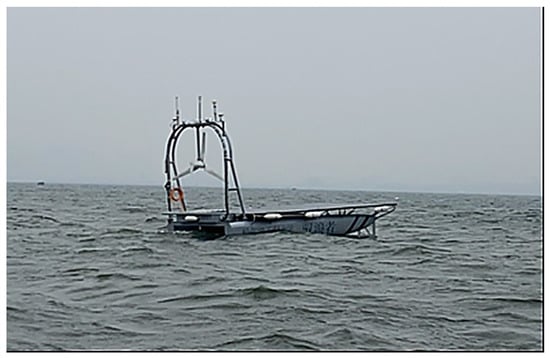
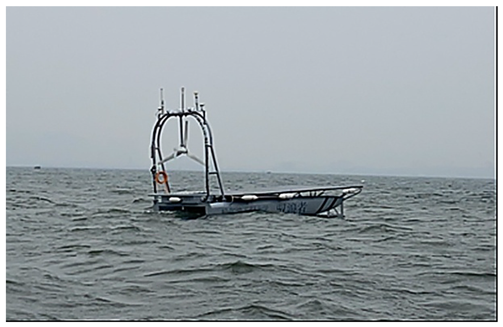
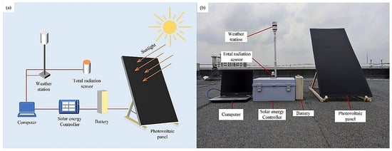
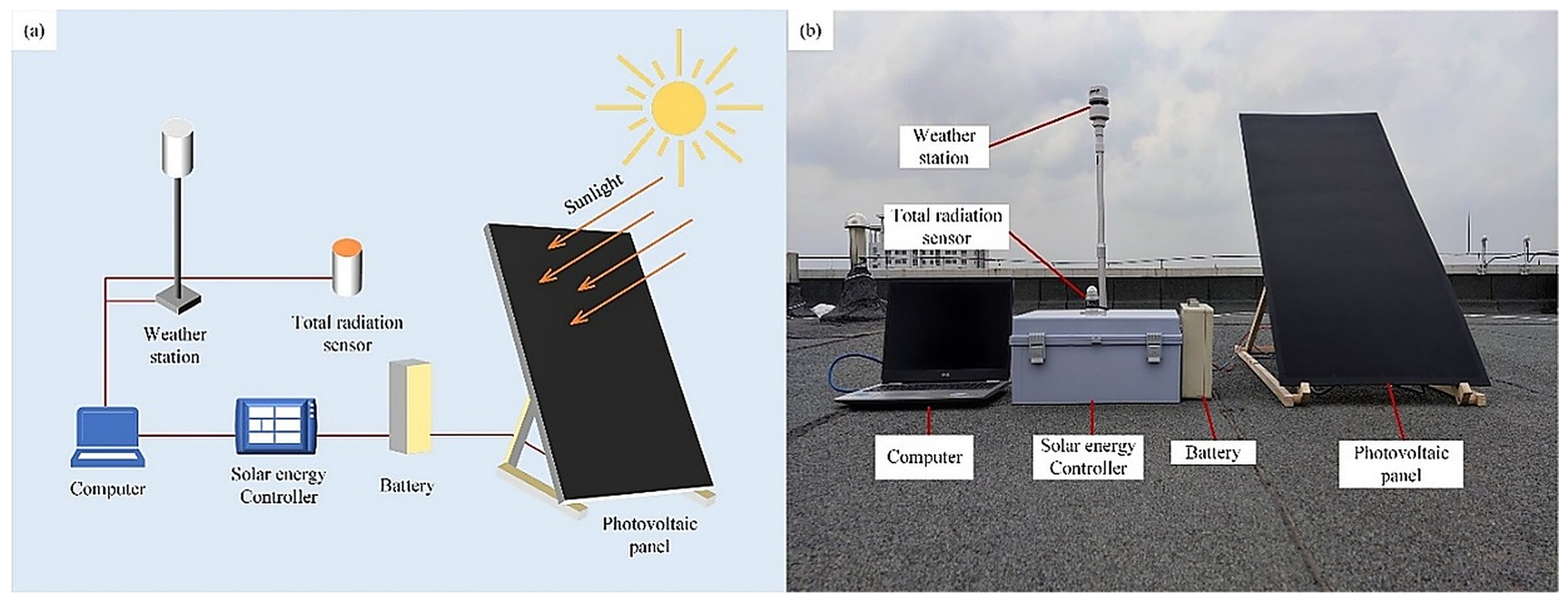
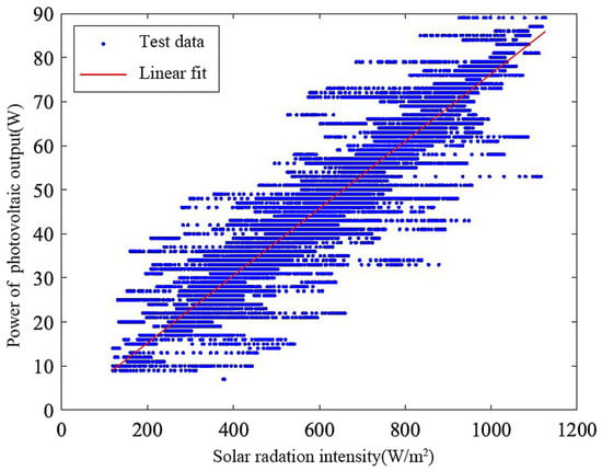
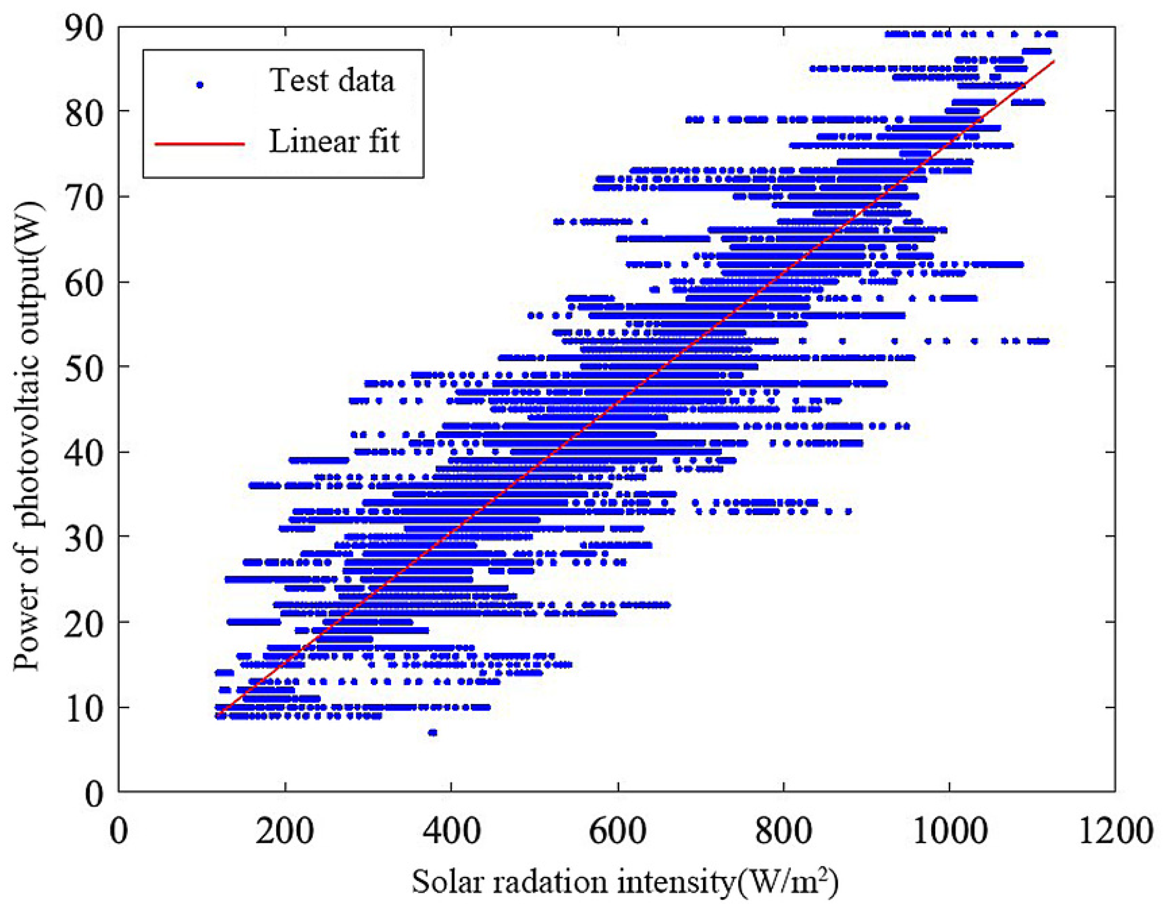
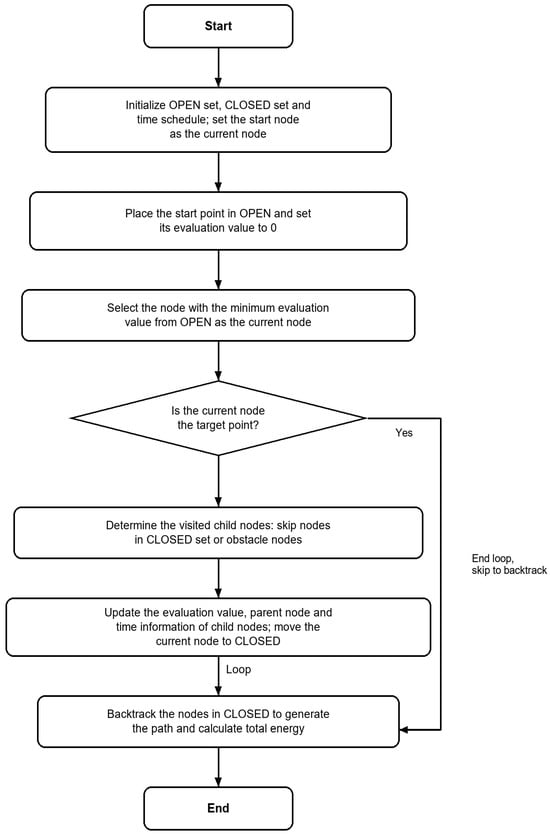
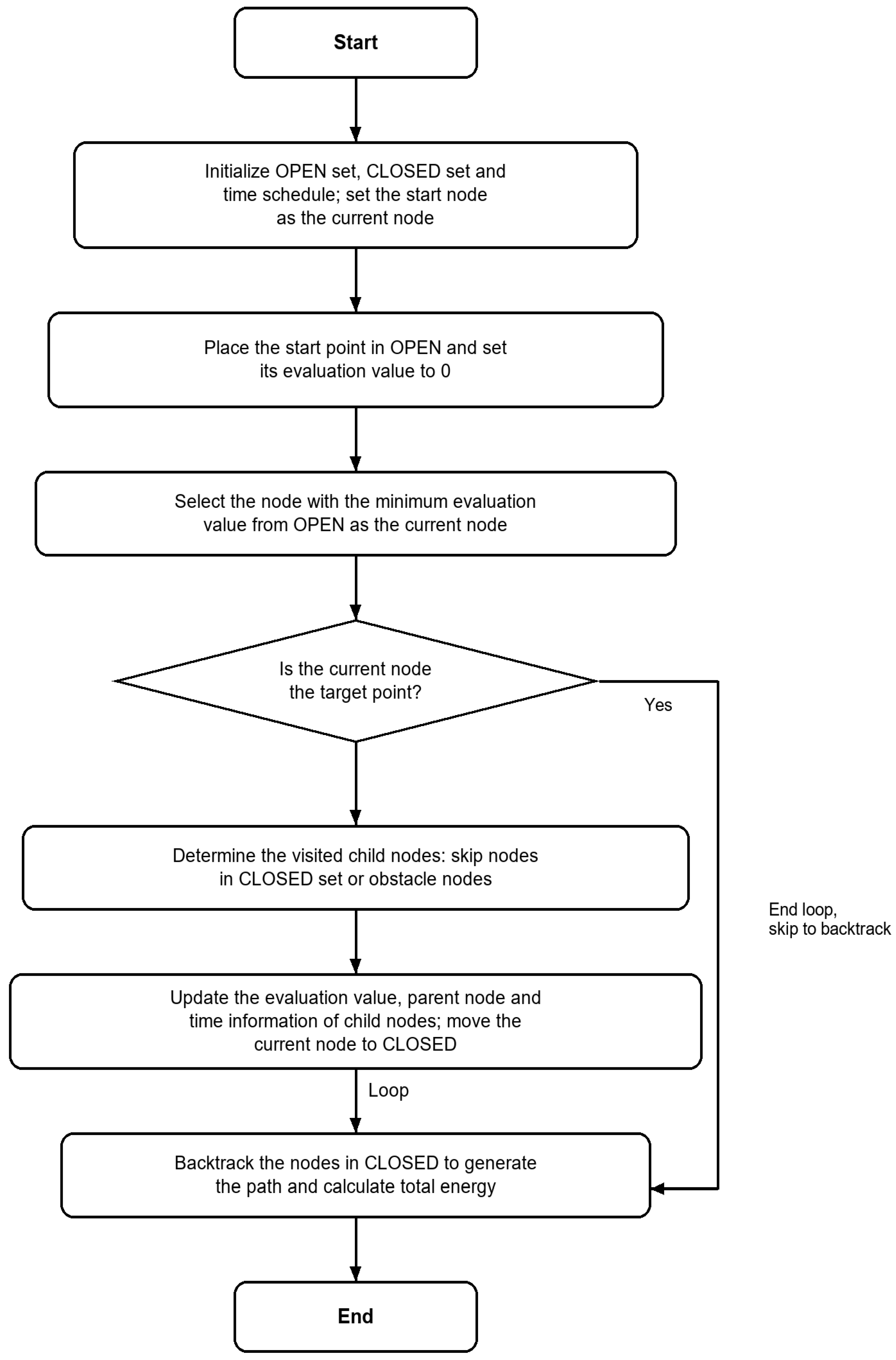
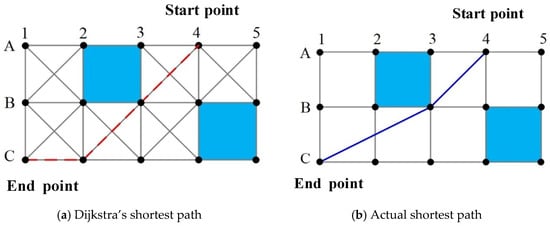
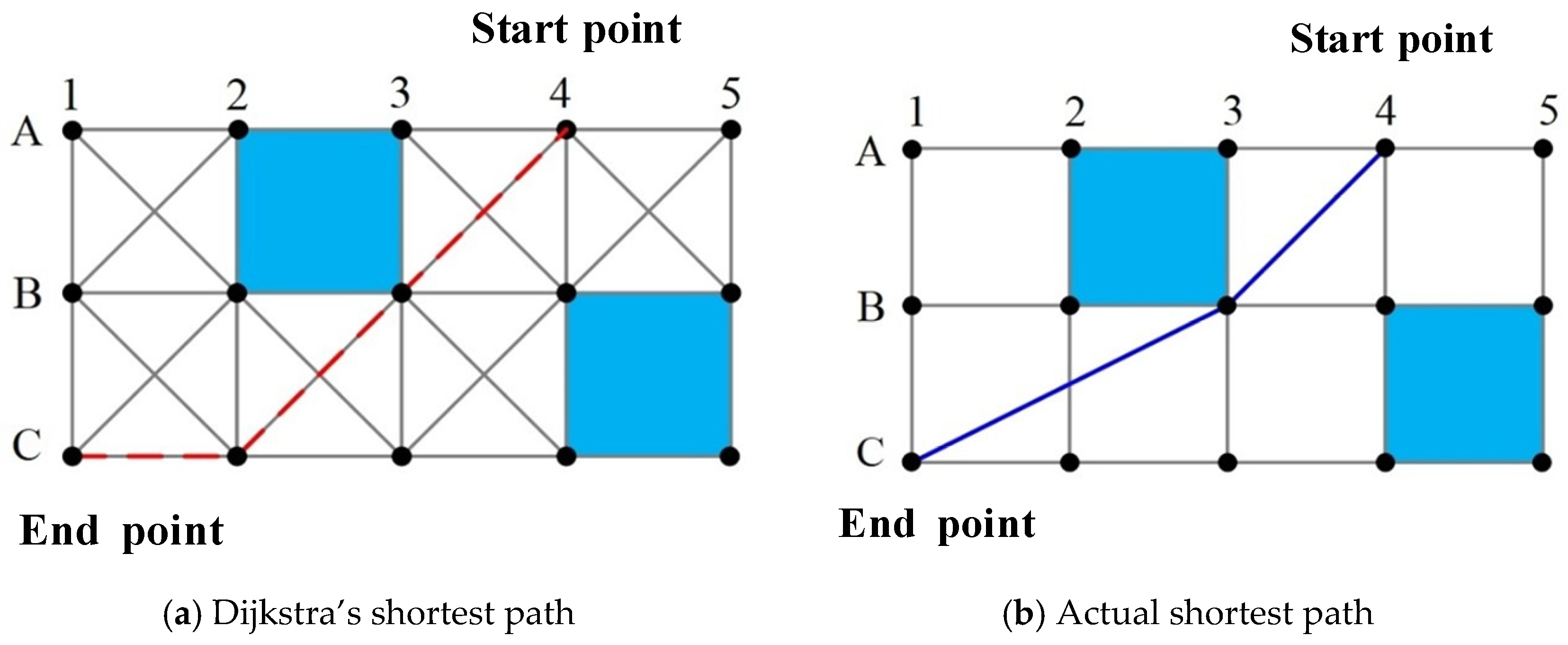
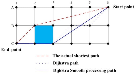
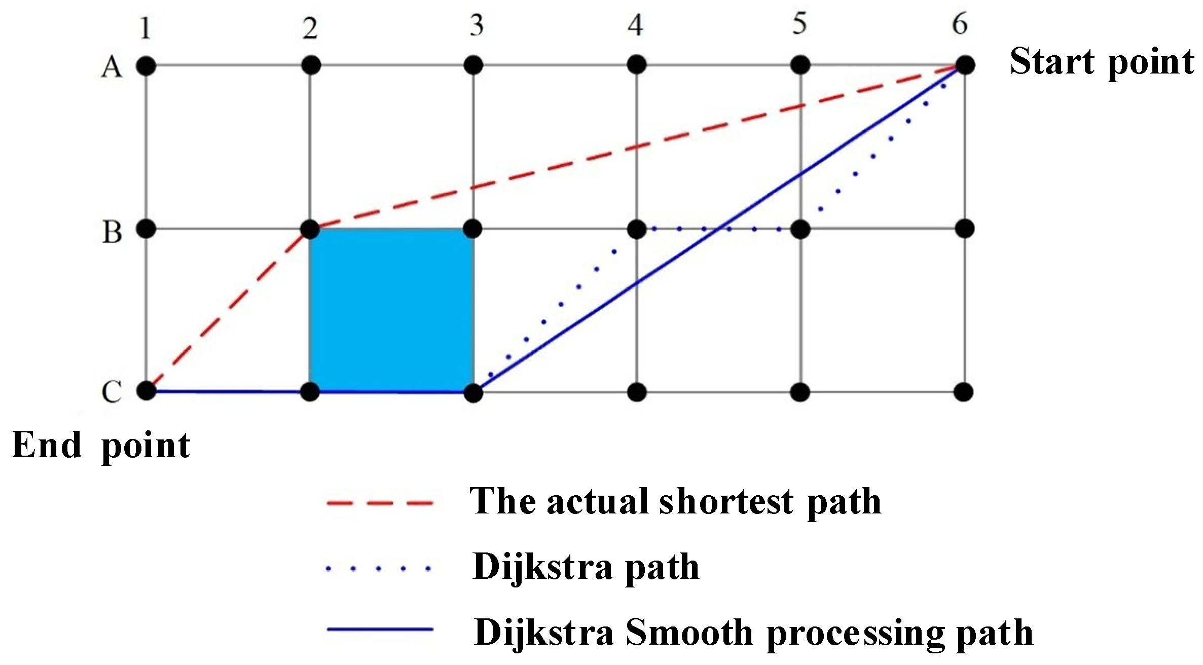
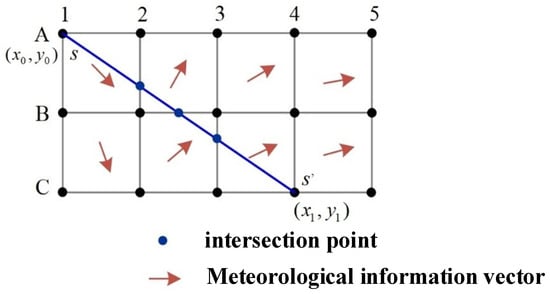
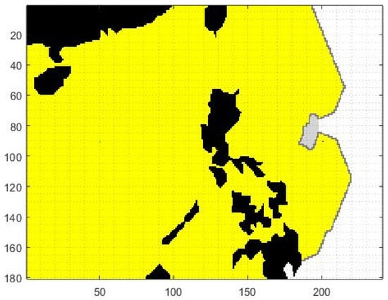
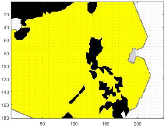
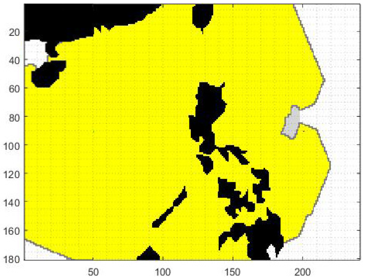
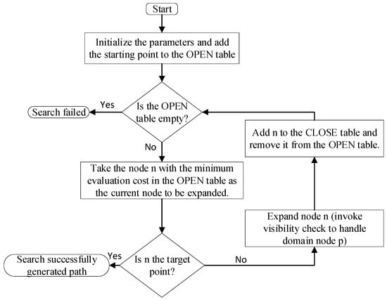
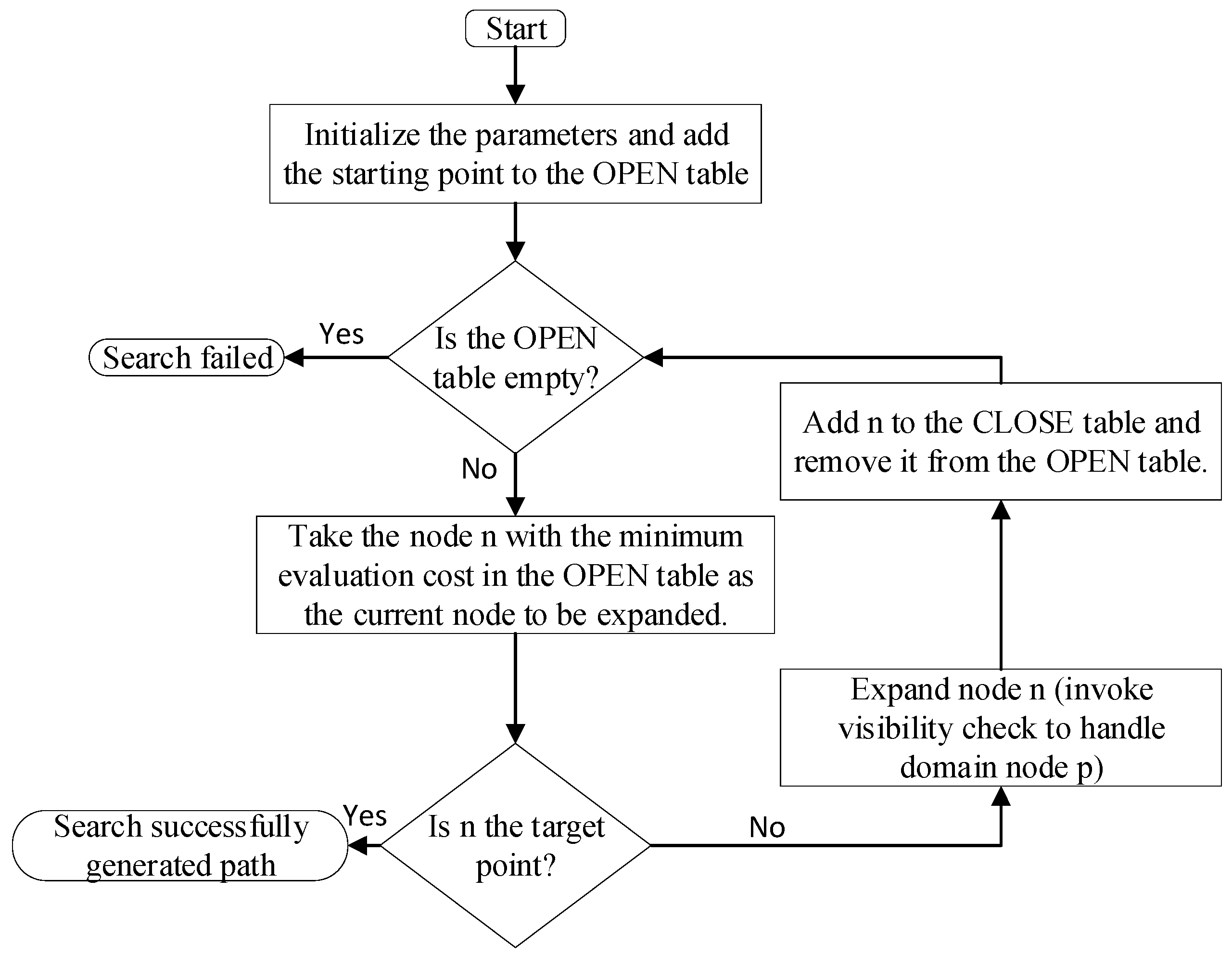
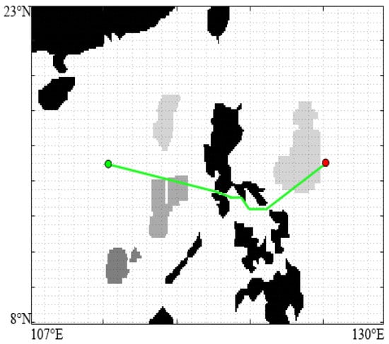
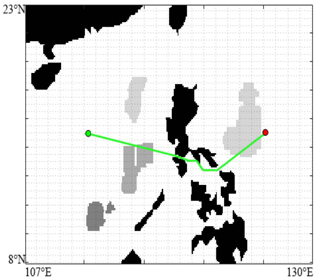
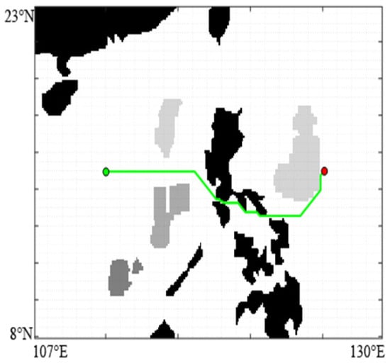
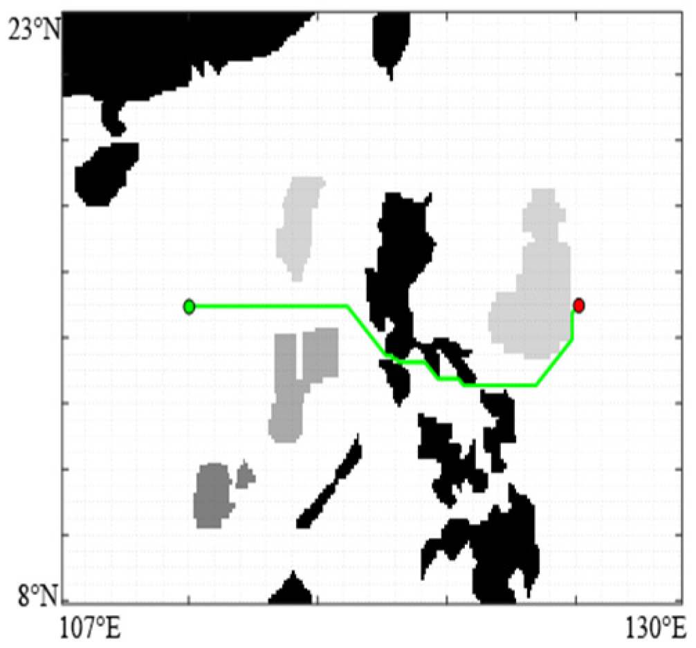
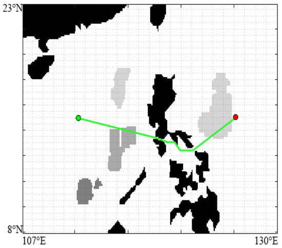
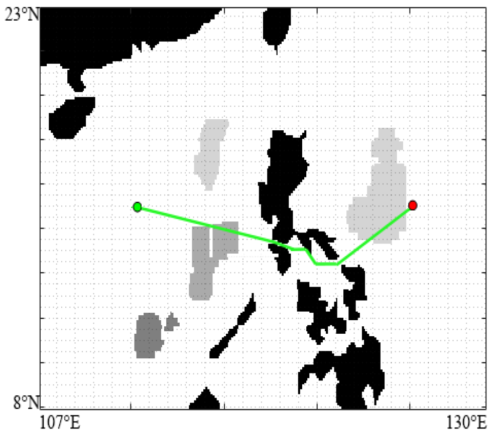
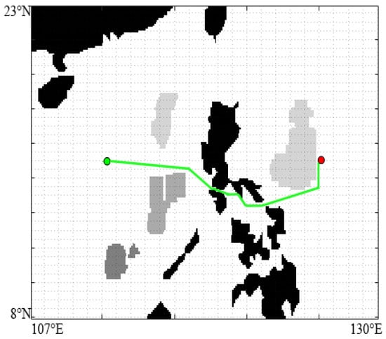
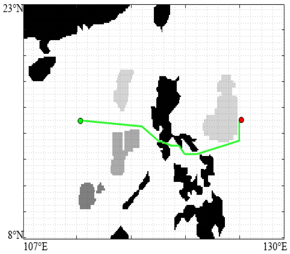
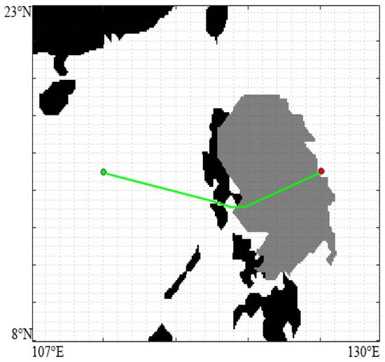
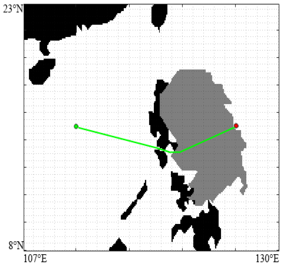
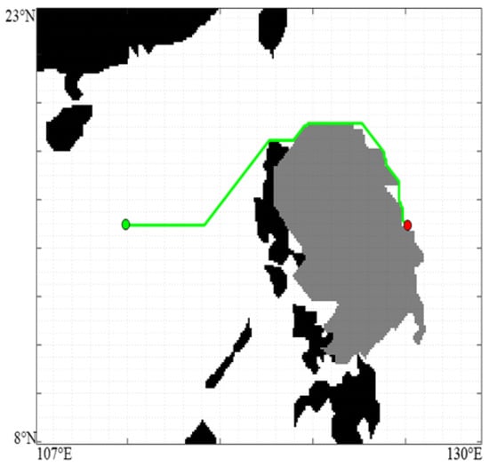
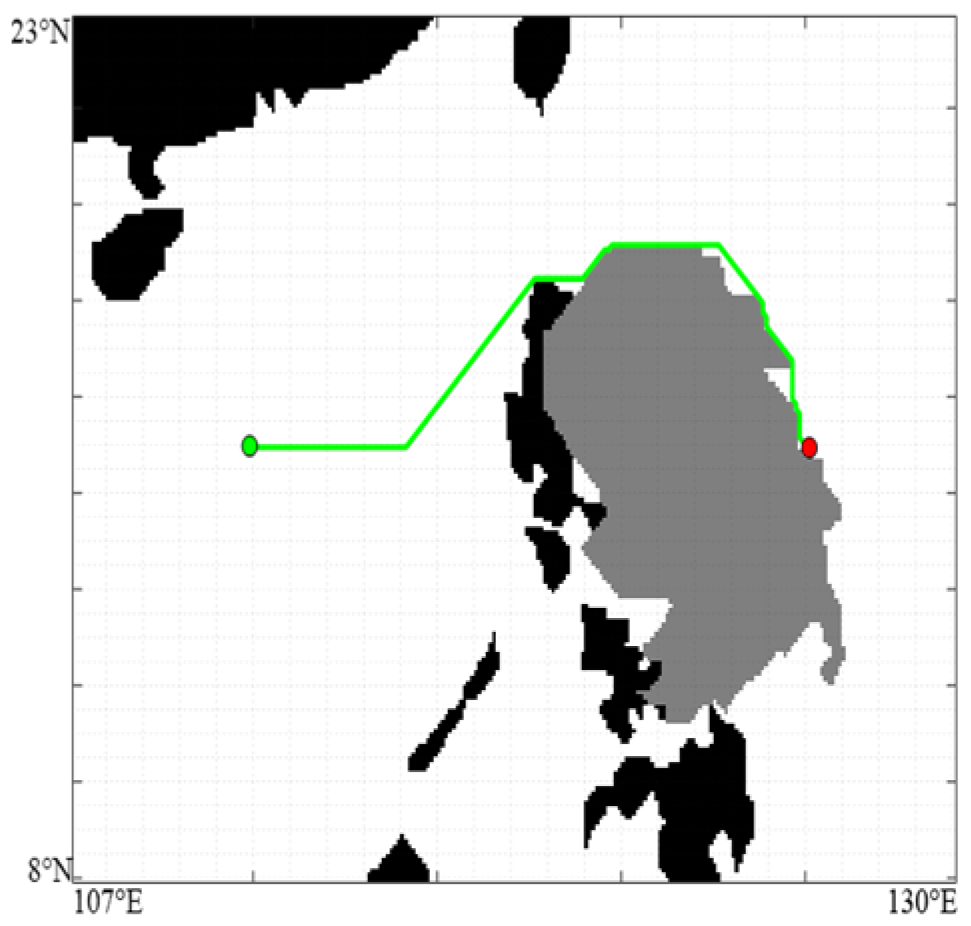
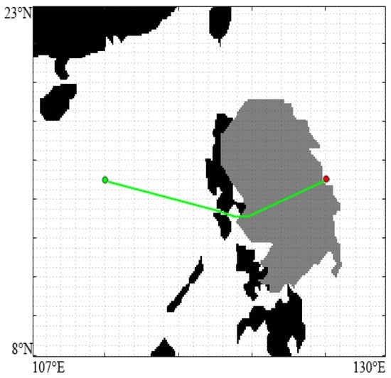
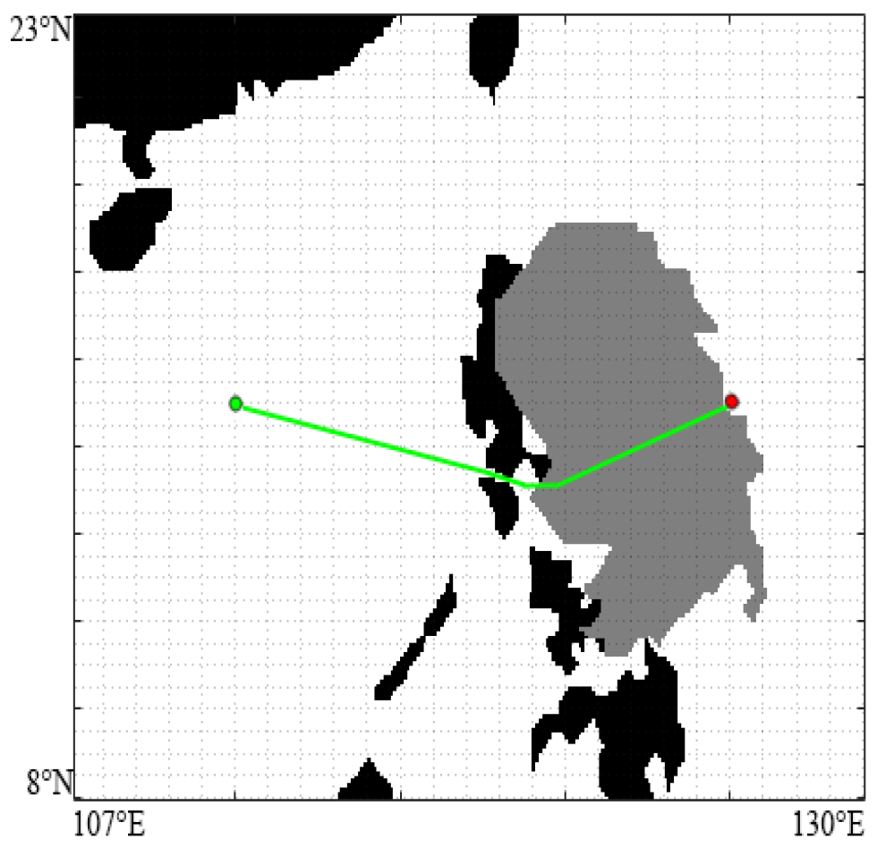
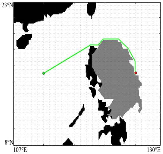
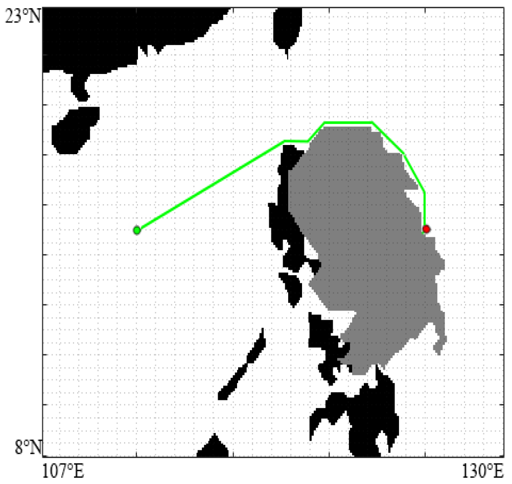
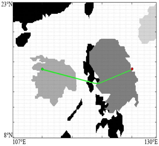
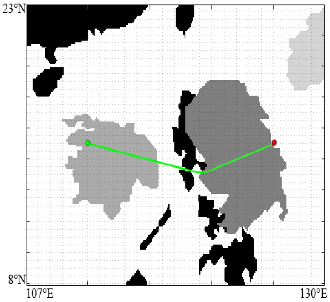
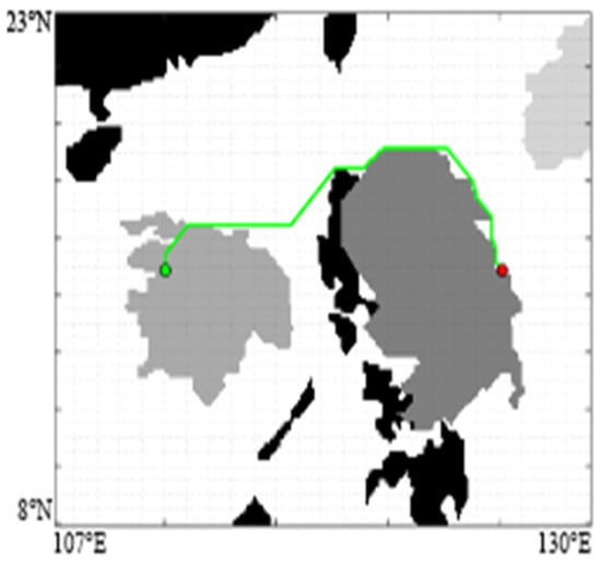
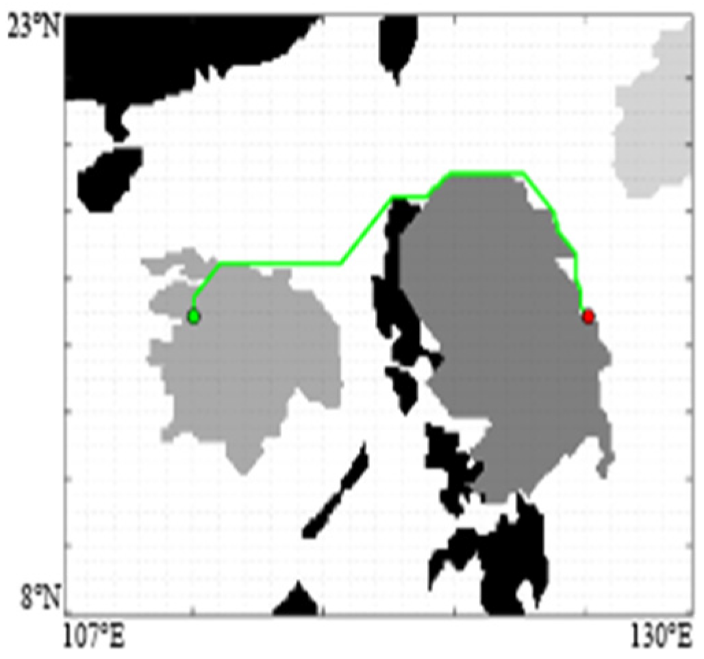
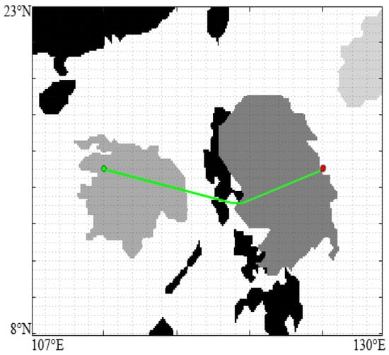
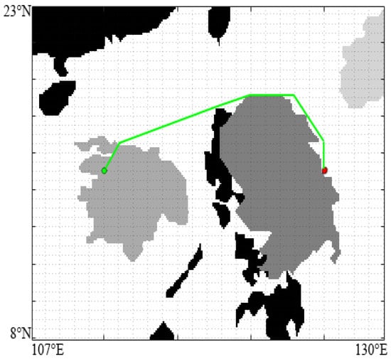
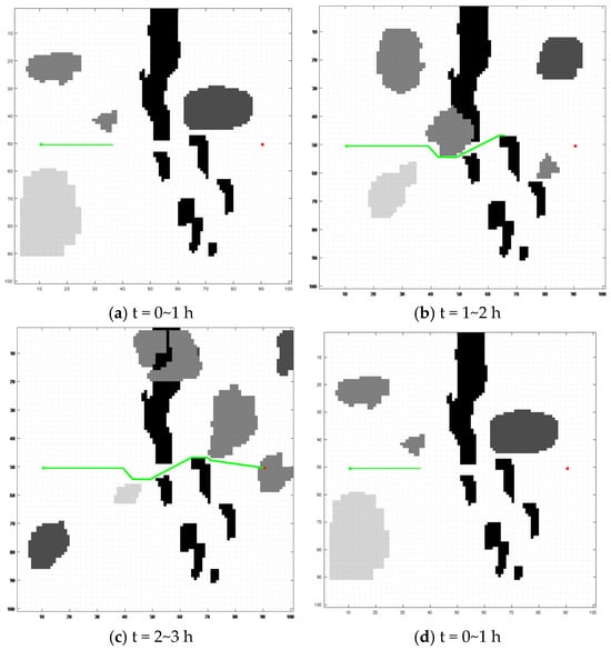
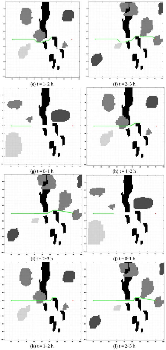
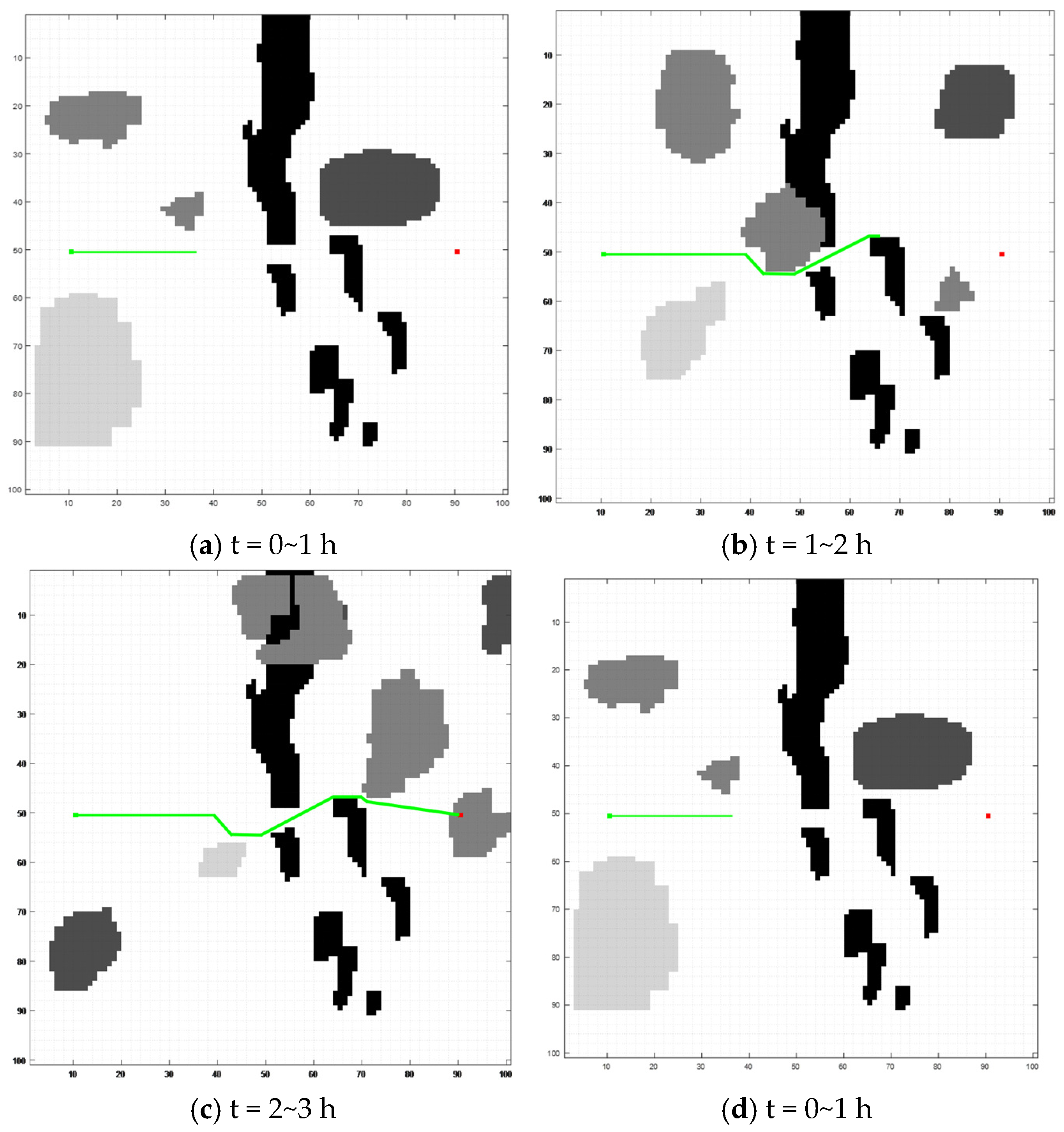
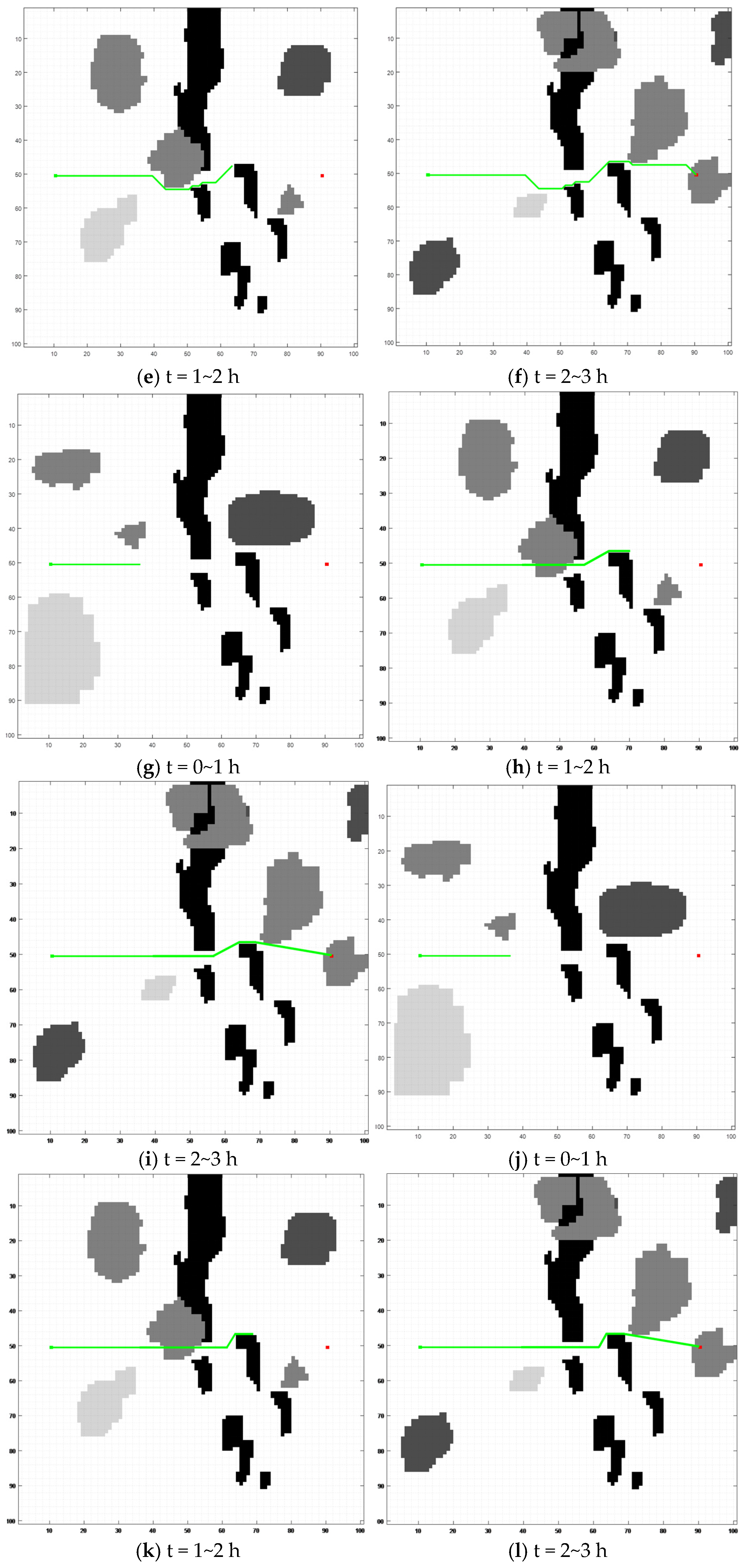
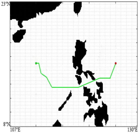
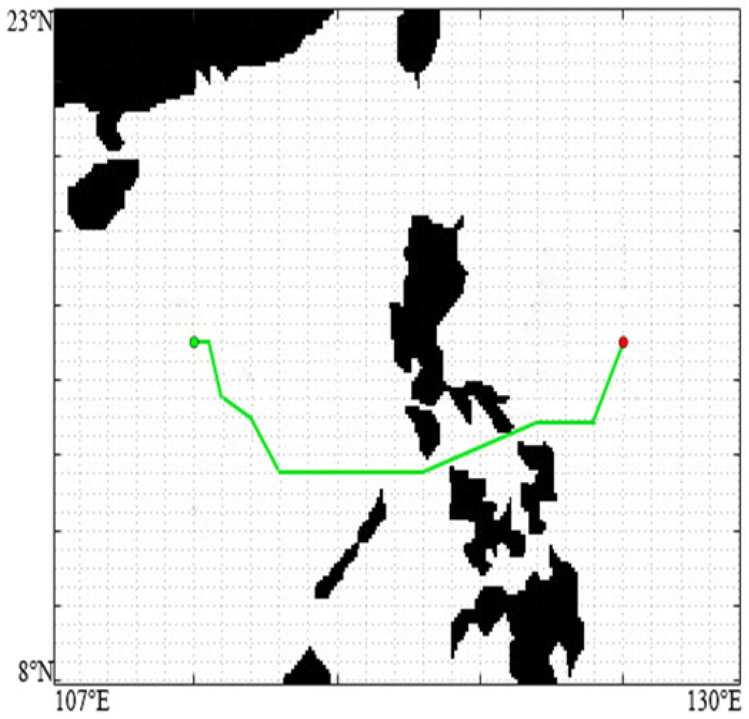
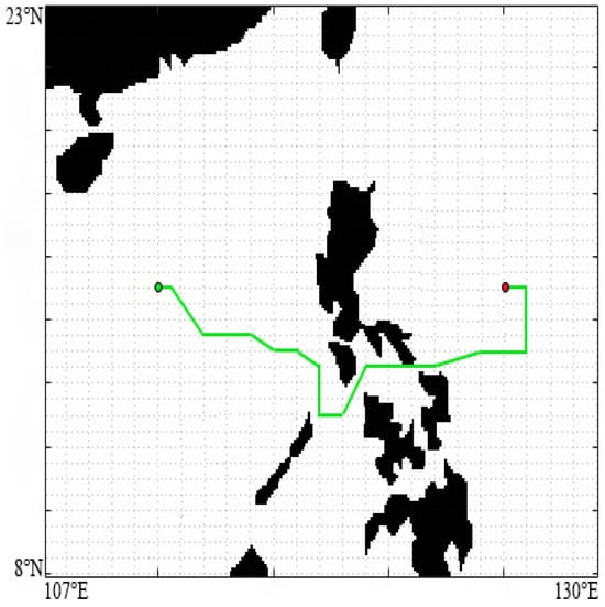
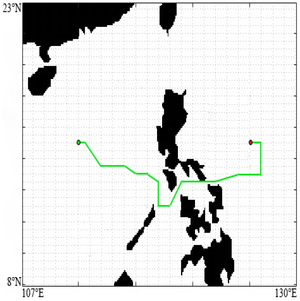
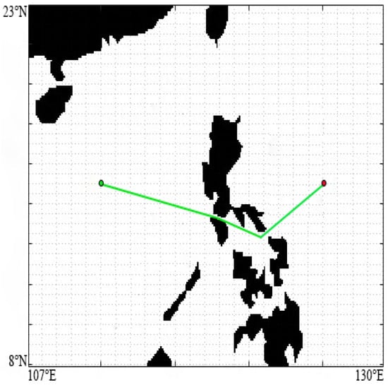
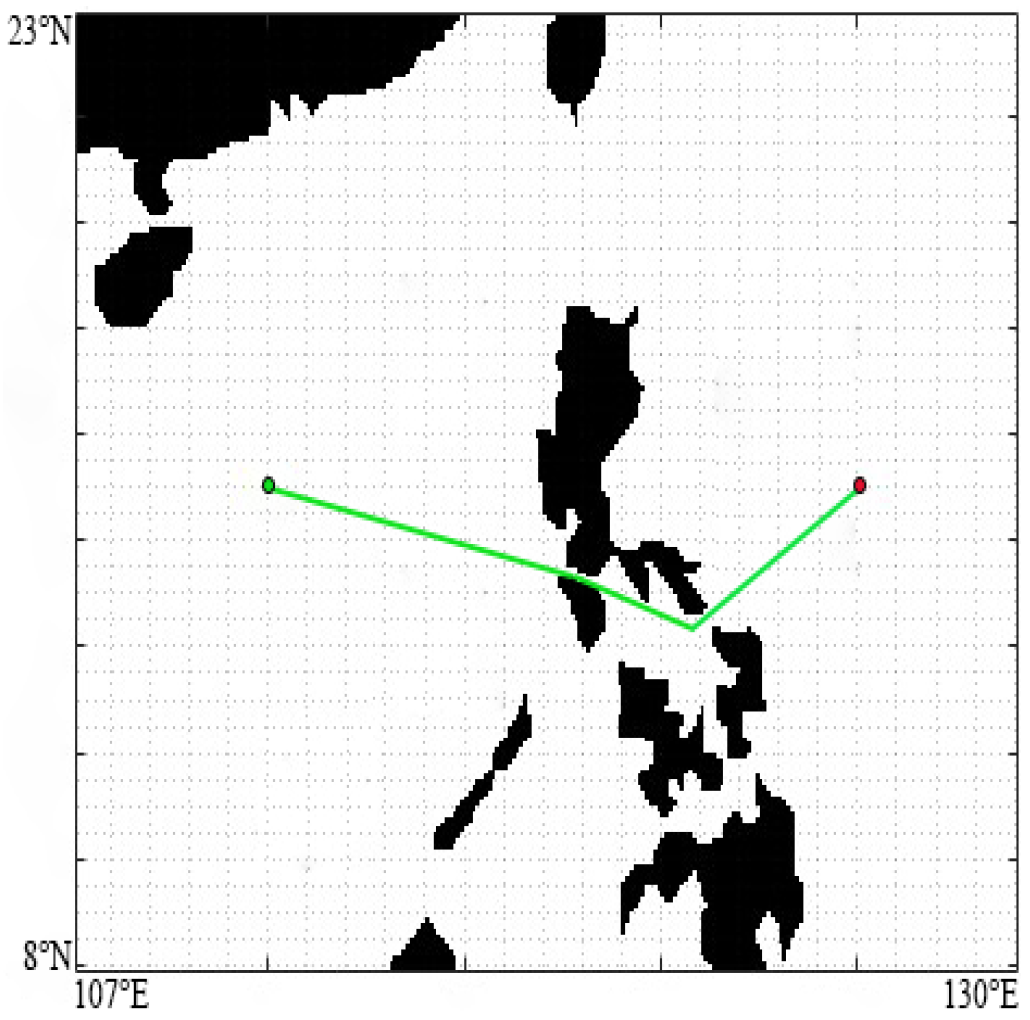
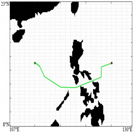
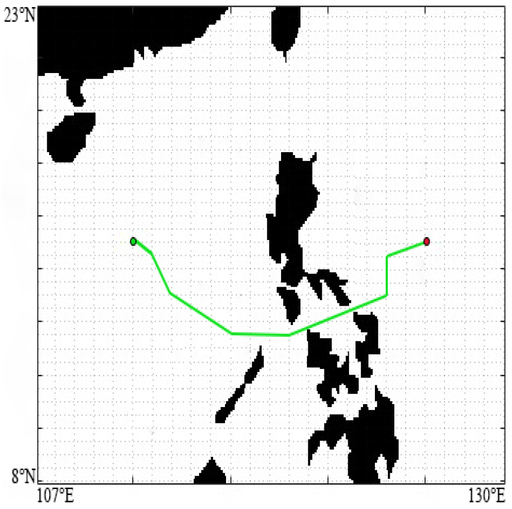

Disclaimer/Publisher’s Note: The statements, opinions and data contained in all publications are solely those of the individual author(s) and contributor(s) and not of MDPI and/or the editor(s). MDPI and/or the editor(s) disclaim responsibility for any injury to people or property resulting from any ideas, methods, instructions or products referred to in the content. |
© 2026 by the authors. Licensee MDPI, Basel, Switzerland. This article is an open access article distributed under the terms and conditions of the Creative Commons Attribution (CC BY) license.