Correlation-Based Temporal Correction of WRF Wind Fields Using Offshore Measurements for Nearshore Wind Resource Assessment

Abstract

Accurate wind estimation is essential for wind resource assessment. In this study, using scanning lidar measurements and high-resolution WRF simulations from two nearshore areas in Japan, we developed two extensions of the Temporal Correction (TC) method, which corrects wind fields generated by the Weather Research and Forecasting (WRF) model using on-site measurements. First, when using a single measurement point for correction, we derived two empirical formulas to predict appropriate correction coefficients based on reference–target correlation coefficients of wind speed obtained from WRF simulations and developed a method (TC-pred) using these formulas. TC-pred was shown to have higher wind speed estimation accuracy and a broader range of applicability than the conventional TC method. Next, we extended the TC-pred method to allow the use of multiple measurement points as references by introducing a weighting formula for each reference point. Wind speed estimation accuracy improved as the number of reference points increased, primarily because the probability of including reference points with high reference–target correlation coefficients increased. This suggests that it is effective for the suppression of wind estimation uncertainty to determine measurement layout such that the correlation coefficient between at least one reference point and each target point in the target area exceeds a certain value.

1. Introduction

During the planning stage of a wind farm, accurate and reliable wind resource assessment is essential, because it underpins energy yield assessment that determines most of the project revenue. In wind resource assessment, the wind conditions at planned turbine locations (hereafter “target points”) are typically inferred by combining wind fields simulated by a wind flow model with wind measurements at a specific on-site location (hereafter the “reference point” or “measurement point”). This procedure is generally referred to as spatial extrapolation, and the resulting estimates form the basis for energy yield calculations. In practical applications of spatial extrapolation, it is common, for example, following the MEASNET guidelines [1], to restrict the assessment to target points located within a radius of approximately 10 km from the reference point.

For onshore wind farms, where terrain and surface roughness effects dominate the spatial variability of the wind field, wind resource assessment is commonly based on steady-state simulations for 12 or 16 wind directions using computational fluid dynamics (CFD) models. Representative examples include the WAsP model widely used in Europe and other areas [2,3] and the MASCOT [4,5] and RIAM-COMPACT [6,7] models developed in Japan.

In contrast, in nearshore areas, particularly in Japan, where offshore wind development has accelerated in recent years [8], the land–sea contrast causes spatial discontinuities not only in terrain and surface roughness but also in atmospheric stability, and an internal boundary layer (IBL) develops along the coast. The formation and structure of such coastal IBLs have been investigated for half a century and have been systematically summarized in textbooks [9]. Recently, the structure of these coastal discontinuities and their influence on the wind field have been examined in detail using site measurements, wind farm operational data, and analyses based on mesoscale meteorological models [10,11,12,13,14,15]. In addition, several studies have compared the performance of CFD and mesoscale meteorological models in nearshore environments and reported that the latter can reproduce wind fields more accurately [16,17]. Consequently, methods that use mesoscale meteorological models, including thermodynamic processes, have become widely adopted for wind-field estimation in nearshore areas.

A representative mesoscale meteorological model used for wind-field estimation is the Weather Research and Forecasting (WRF) model [18] (e.g., [19,20,21]). WRF can reproduce three-dimensional atmospheric fields that include thermodynamic processes and, in particular, has been shown to capture phenomena such as sea-breeze circulations and low-level jets (e.g., [22,23]), making it well suited for wind estimation in nearshore areas.

However, although WRF can generate time series of wind speed and direction, it is typically run without directly using site-specific measurements as constraints, so systematic biases and random errors remain. To reduce these model errors, several correction techniques have been proposed. Examples include observational nudging [24,25,26,27], a data assimilation technique available in WRF that sequentially incorporates observational data into the model integration; the directional extrapolation method, in which directional wind-speed ratios and wind-direction offsets equivalent to CFD results are derived and applied following essentially the same procedure as CFD-based spatial extrapolation [28,29]; and the Temporal Correction (TC) method proposed in our previous study, Maruo and Ohsawa (2025) [30], which corrects the WRF wind vector at each target point and time step using the wind error vector at a reference point.

In our previous study, Maruo and Ohsawa [30], we examined spatial extrapolation from a coastal onshore reference point to offshore target points (so-called land–offshore extrapolation). Using datasets from four nearshore sites in Japan, we compared the performance of the correction methods mentioned above and showed that the TC method yielded the smallest bias in long-term mean wind speed. However, the validation was restricted to pairs of reference and target points with a correlation coefficient $r \ge 0.85$, and it was also suggested that, for $r < 0.85$, the estimation accuracy of TC could be lower than that of “raw” WRF model results without any on-site measurements, in terms of time series correlation. To address this issue, Maruo and Ohsawa [30] pointed out the need to adjust the correction coefficient $\alpha$, which is applied to the WRF wind error vector at the reference point, according to the relationship between the two locations.

In the present study, we extend the TC method proposed in our previous work and, for the case of a single-point reference, develop a formulation that determines the correction coefficient $\alpha$ based on the relationship between the reference and target points so as to minimize the estimation error and evaluate the resulting estimation accuracy.

In this formulation, we derive empirical relationships that estimate a “measurement-equivalent” inter-point correlation from the correlation derived from WRF and predict the appropriate correction coefficient α as a function of this correlation, thereby clarifying the relationship between $r$ and $\alpha$.

In recent years, multiple wind measurement points using scanning lidars and other instruments have increasingly been conducted in wind measurement campaigns. In this study, we focus on offshore–offshore extrapolation, in which offshore measurement points are used as reference points to estimate the wind conditions at unmeasured offshore target points. When multiple reference points are available, the representativeness of each point must be taken into account when estimating the wind at the target points. We therefore extend the TC method to a multiple-reference-point framework by introducing a scheme that reflects the representativeness of each reference point, and evaluate its accuracy. Considering representativeness in this way not only improves wind estimation accuracy but also provides insights for the design of a measurement layout, such as where measurement points should be located and how many points are required.

The objective of this study is to enhance the applicability of the TC method in nearshore areas. Specifically, this study has the following three aims:

• To construct a framework that predicts the appropriate correction coefficient $\alpha$ in the TC method with a single reference point, based on the relationship between the reference and target points, and to evaluate its wind estimation accuracy;
• To extend the TC method to a multiple-reference-point framework and to evaluate its wind estimation accuracy; and
• To interpret the single- and multiple-reference-point validation results in terms of correlation-based representativeness and effective correction range, and to discuss implications for nearshore measurement-point layout design.

The remainder of this paper is organized as follows. Section 2 describes the two study nearshore sites and measurement datasets, as well as the WRF configuration, and provides an overview of the TC method. Section 3 derives a framework to predict the appropriate correction coefficient α based on the relationship between the reference and target points and examines the wind estimation accuracy of the extended TC method with a single reference point. Section 4 extends the TC method to multiple reference points using the derived relationships and evaluates the wind estimation accuracy in the multiple-reference-point case. Section 5 discusses practical issues related to the application of the proposed method and implications for measurement network design. Section 6 concludes the paper.

2. Materials and Methods

2.1. Sites and Measurement Data

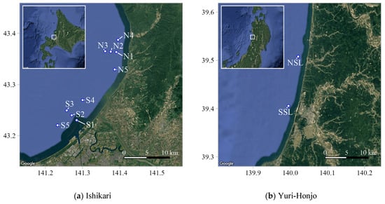
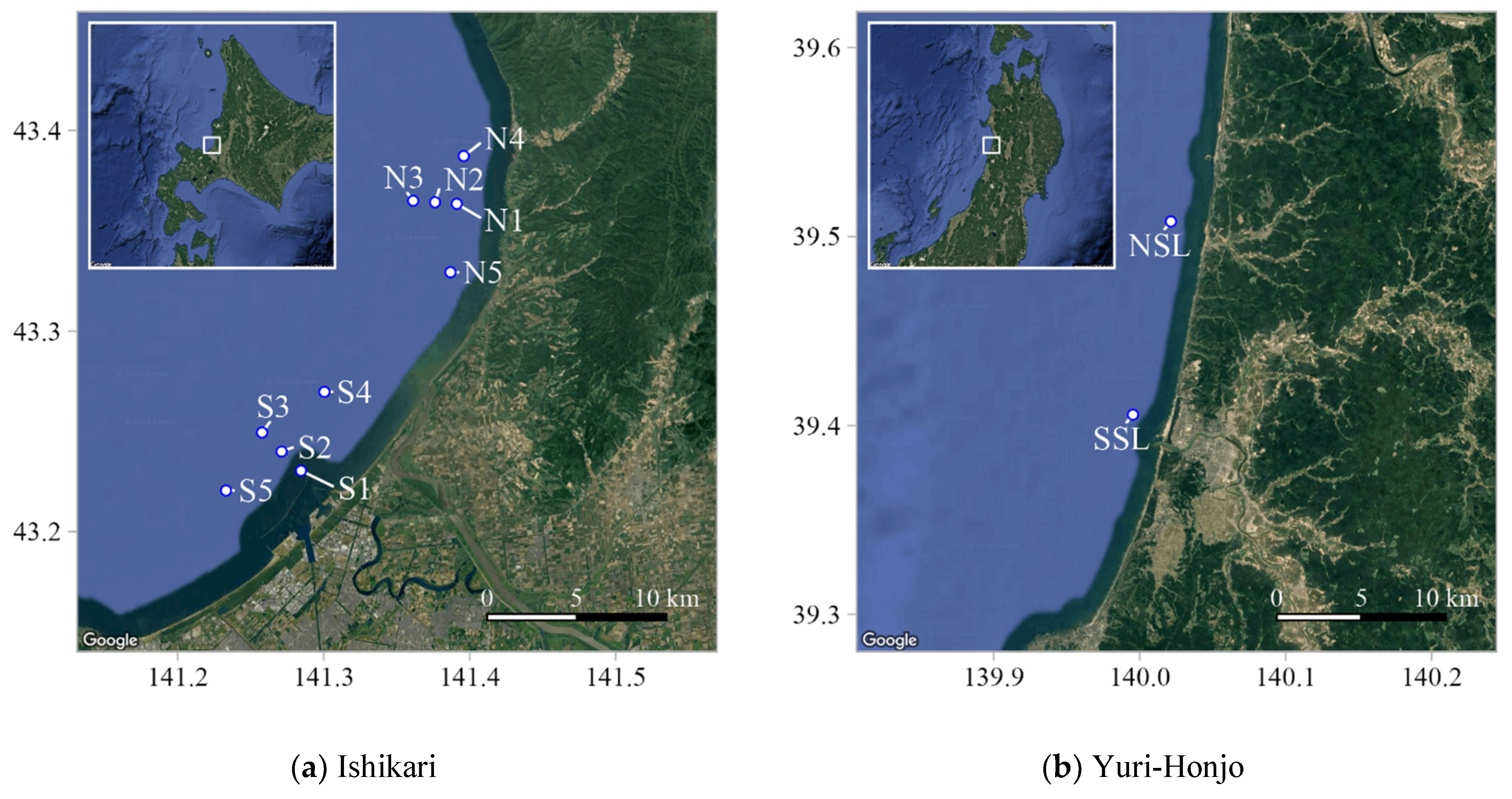
In this study, we used wind measurement data obtained from two nearshore sites in Japan: off Ishikari Port in Hokkaido (hereafter “Ishikari”) and offshore of Yuri-Honjo City in Akita Prefecture (hereafter “Yuri-Honjo”). These two sites represent typical development areas for offshore wind energy projects along the Sea of Japan coast. The measurement points at each site are shown in Figure 1. Detailed information on the instrumentation, measurement heights, and installation conditions is summarized in Table 1. The site-specific descriptions below refer to these figures and tables.

Figure 1. Locations of the nearshore study sites and on-site wind measurement points. (a) Ishikari (Hokkaido): offshore measurement points (N1–N5 and S1–S5) observed at 142 m ASL using dual-scanning lidars. (b) Yuri-Honjo (Akita): offshore measurement points NSL and SSL (approximately 11.6 km apart) observed at 40, 100 and 160 m ASL using onshore scanning lidars. Insets show the site locations in Japan.

Table 1. Measurement configuration. AMSL: Above Mean Sea Level; SSL: Single Scanning (Doppler) LiDAR system; DSL: Dual Scanning (Doppler) LiDAR system; RHI: Range Height Indicator; PPI: Plan-Position Indicator; SR: Sampling Rate; LOS: Line-of-Sight.

Site	Point	Method (Scan)	Equipment	Specification and Settings of Scan	Height Used for Analysis (AMSL)
Ishikari	N1–N5, S1–S5	DSL (RHI)	Windcube 400S×2 (Measuring offshore from shore)	SR: 1 Hz Gate Length: 50 m	142 m (1 height)
Yuri-Honjo	NSL, SSL	SSL (PPI)	StreamLine XR (Measuring offshore from shore)	SR: 1 Hz Gate Length: 90 m, Sector size: 60°, consisting of 5 LOS	40 m, 100 m, 160 m (3 heights)

Figure 1a shows the measurement points at Ishikari. Offshore wind conditions at 142 m above sea level were measured at ten points (N1–N5 and S1–S5) using two pairs of dual-scanning lidars (Windcube 400S; Vaisala, Finland) installed on the northern and southern coasts. The northern dual-scanning pair was configured to scan the five northern offshore points (N1–N5), whereas the southern pair scanned the five southern offshore points (S1–S5). Around the northern coast, five offshore points (N1–N5) were arranged as follows: N1 is located approximately 3 km offshore, N2 and N3 are located along the cross-shore direction at intervals of 1.2 km from N1, and N4 and N5 are located approximately 2.6 km to the north and 3.8 km to the south of N1 along the coastline. Around the southern coast, five offshore points (S1–S5) were arranged in a similar manner: S1 is located approximately 2.5 km offshore, S2 and S3 are located along the cross-shore direction at intervals of 1.5 km from S1, and S4 and S5 are located approximately 4.0 km to the north and 3.5 km to the south of S2 along the coastline. Under the measurement configuration, two scan patterns were alternated during each hour. During the first 30 min, the lidars were operated to retrieve winds at N1, N2, N3, S1, S2 and S3 (hereafter referred to as Group A), and during the latter 30 min, they were operated to retrieve winds at N1, N4, N5, S1, S4 and S5 (Group B). S5 was excluded from the present analysis because it is located close to existing offshore wind turbines and was considered potentially affected by turbine wakes. The potential wake influence on S1–S3 was also checked because the existing turbines are located to the south to southwest of these points, which are within approximately 20 rotor diameters of the nearest turbines under specific wind directions. The rotor diameter of the turbines is 167 m, which is hereafter denoted as D. The distances from the nearest turbines to S1, S2, and S3 are approximately 1.9, 1.9, and 2.8 km, corresponding to 11.4D, 11.4D, and 16.8D, respectively. However, the turbines could have affected the measurements only after 10 September 2023, when construction was completed. Wind roses based on the validation samples from 10 September 2023 to 29 February 2024 showed that winds from the turbine-side sectors were very rarely observed at S1–S3. Therefore, although possible wake effects under limited wind directions cannot be completely ruled out, the wind direction distributions did not indicate a clear need to exclude S1, S2, and S3 from the analysis.

Horizontal wind vectors at each offshore point were reconstructed from pairs of line-of-sight (LOS) wind speeds using the dual-LOS method described in a previous study [31,32]. In each scan cycle, range–height indicator (RHI) scans sampled three measurement points, and 18 LOS samples (1 LOS per 1 s) were obtained at each point over a 1-min interval. For each 10-min period, LOS samples from consecutive scans were aggregated, and outliers exceeding ±3σ from the 10-min mean LOS wind speed were removed. Horizontal wind vectors were then reconstructed, and 10-min mean wind speed and direction were computed. Only 10-min values with at least 60 valid 1-s horizontal wind speed and direction samples at each point were retained. This study used these 10-min mean wind speeds and directions for the continuous 12 months from 1 March 2023 to 29 February 2024 (JST). For the statistical analysis, we therefore considered Group A and Group B separately and used only time stamps for which all selected points in a given group had valid data. As a result, the numbers of valid 10-min samples were 18,704 (data availability: 35.5%) for Group A and 16,265 (30.9%) for Group B.

Figure 1b shows the measurement points off Yuri-Honjo, located in the southern part of Akita Prefecture. Two single-scanning lidars (Streamline XR) were installed onshore along the northern and southern coastlines, respectively. These lidars measured wind conditions at two offshore points, NSL and SSL, located approximately 2 km from the coast, at three heights: 40 m, 100 m and 160 m above sea level. The horizontal distance between NSL and SSL is approximately 11.6 km. Horizontal wind vectors were retrieved using the single-LOS reconstruction method described in a previous study [32]. For each 10-min period, only those records with at least seven out of a maximum of twelve available wind-vector samples were used. The analysis period covered 12 months from 1 February 2020 to 31 January 2021 (JST), resulting in 31,647 valid 10-min samples (data availability: 60.0%).

2.2. Model and Methods for Time Series Estimation

This section provides an overview of the three methods used in this study to estimate wind speed. We confirmed in our previous study that, for wind direction estimation, none of the methods showed a practically significant difference in performance; therefore, this issue is not addressed in this study.

2.2.1. WRF Control Simulation Without On-Site Measurement Data (CTRL)

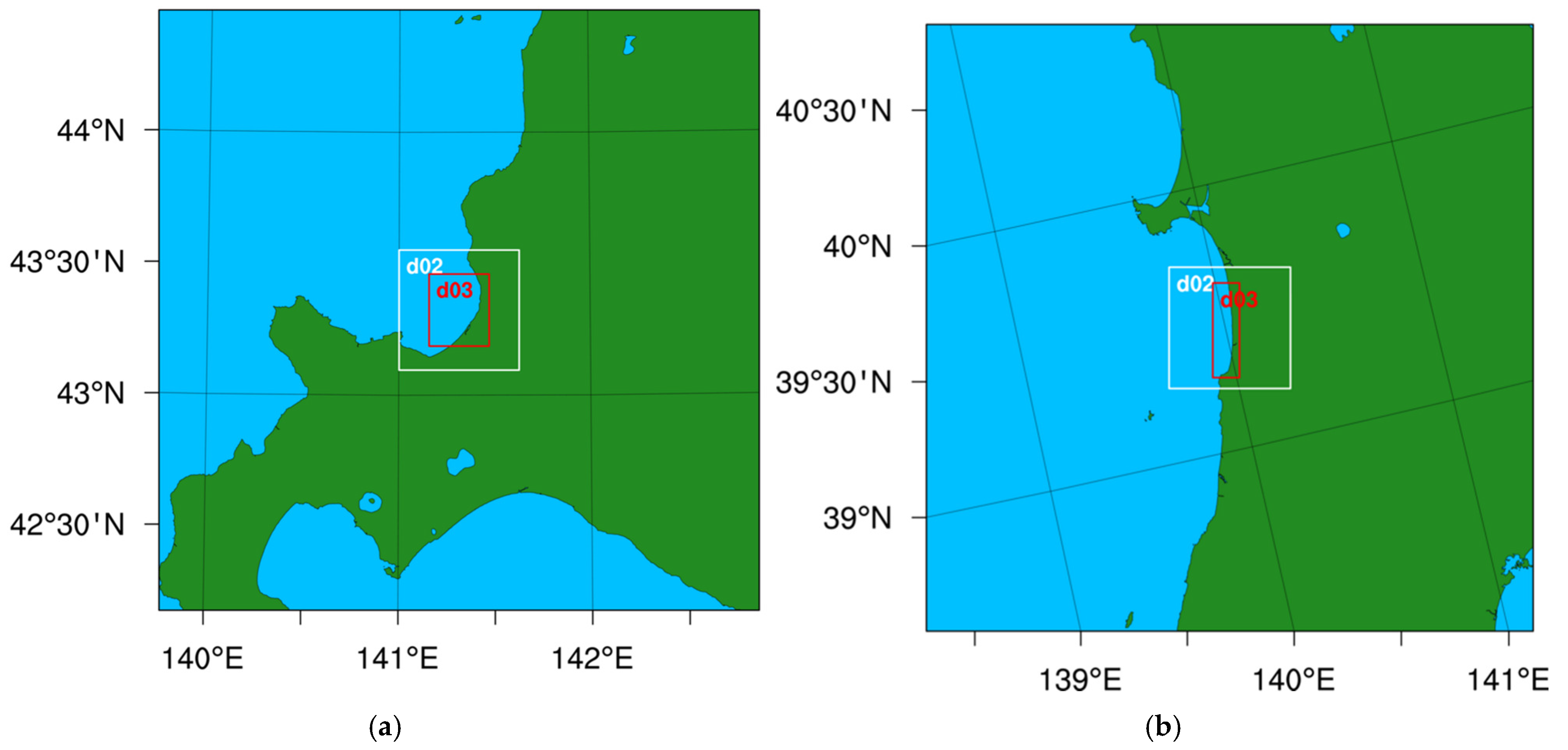
The first estimation method is a control simulation using a mesoscale meteorological model without on-site measurement data (hereafter CTRL). In this study, the Weather Research and Forecasting (WRF) model (version 4.3.3) was used as the mesoscale model. WRF is a non-hydrostatic and fully compressible numerical weather prediction model that is widely used in wind energy applications. The model configuration is based on the NeoWins project and related studies [33] and closely follows that used in our previous study [30]; the main settings are summarized in Table 2. Separate model domains were set up for each target site, and the horizontal grid spacing was refined from 2.5 km to 0.1 km by a factor of five through two nested domains (Figure 2). In d02 and d03, four-dimensional data assimilation (FDDA) was applied only above approximately 2 km AGL to prevent large-scale meteorological drift while avoiding constraints from the coarser input data in the lower layer relevant to wind-resource assessment, including turbine-rotor heights, IBL development, and Planetary Boundary Layer (PBL). Each continuous simulation run covered up to 8 days for Ishikari and 9 days for Yuri-Honjo, including a 1-day spin-up period. Time series for the CTRL method were obtained by extracting the wind speed and direction at the target point and height from the WRF simulation results via spatial interpolation of the model grid. Specifically, the four grid points surrounding the target point were vertically interpolated to the target height using a logarithmic interpolation and then horizontally interpolated to the target point using a bilinear scheme.

Table 2. WRF configuration.

Model Version	WRF (ARW)V4.3.3
Period	Ishikari	1 March 2023~29 February 2024 (1 year)
	Yuri-Honjo	1 February 2020~31 January 2021 (1 year)
Input data	Met	JMA-LFM (1 hourly, 0.02º × 0.025º)
	Soil	NCEP FNL (6 hourly, 1º × 1º)
	SST	Met Office OSTIA (Daily, 0.05º × 0.05º)
Terrain data	Elevation	METI, NASA ASTER-GDEM
	Land use	MEIT, MLNI land use subdivision mesh
	Roughness Table	Based on JMA, except that mixed forest is set to 2.0 m instead of the JMA value of 3.0 m.
Grid spacing	d01	2.5 km (100 × 100)
	d02	0.5 km (100 × 100)
	d03	0.1 km (Ishikari: 250 × 300/Yuri-Honjo: 110 × 390)
Vertical levels		40 layers (Surface to 100 hPa)
Physics options	Shortwave	Dudhia scheme
	Longwave	Rapid Radiative Transfer Model scheme
	Microphysics	Ferrier (new Eta) scheme
	PBL	Mellor-Yamada-Janjič (Eta operational) scheme
	Surface layer	Monin-Obukhov (Janjic Eta) scheme
	Land surface	Noah Land Surface Model scheme
	Cumulus Parameterization	Kain-Fritsch (new Eta) scheme (only d01)
FDDA	d01	Grid nudging enabled for (u, v, θ, q)
	d02, d03	Grid nudging enabled for (u, v, θ, q) above the 13th model level (i.e., applied above approximately 2 km AGL)

Figure 2. WRF simulation domains: (a) Ishikari and (b) Yuri-Honjo. The full map corresponds to d01; the green and light-blue areas indicate land and sea, respectively; the white and red boxes indicate d02 and d03, respectively.

2.2.2. Temporal Correction Method (TC)

The second estimation method is the temporal correction (TC) method proposed in our previous study. This method is an offline correction applied after the model simulation, in which the wind vector at each target point at time $t$ is adjusted using the wind error vector between the measurement and the model-simulated result at the same time $t$ at a single reference point. The formulation of TC (Figure 3) is as follows:

Figure 3. Schematic illustrating the TC method.

Figure 3. Schematic illustrating the TC method.

$${\mathit{V}}_{tgt}^{EST}(x, y, z, t)={\mathit{V}}_{tgt}^{WRF}(x, y, z, t)+{\mathit{ϵ}}_{ref}(x_n, y_n, z_n, t)$$

(1)

$${\mathit{ϵ}}_{ref}(x_n, y_n, z_n, t)=\alpha {∆\mathit{V}}_{ref}(x_n, y_n, z_n, t)=\alpha \left({\mathit{V}}_{ref}^{Meas}\right(x_n, y_n, z_n, t)-{\mathit{V}}_{ref}^{WRF}(x_n, y_n, z_n, t\left)\right)$$

(2)

where $\mathit{V}$ represents the horizontal wind vector (10-min values in this study), $x$, $y$ and, $z$ represent coordinate point of a target point, $x_n$, $y_n$ and, $z_n$ represent coordinate point of reference point $n$, $t$ represents a time stamp, ${\mathit{V}}_{tgt}^{EST}$ represents the estimated wind vector at the target point, ${\mathit{V}}_{tgt}^{WRF}$ represents the model-simulated wind vector at the target point, ${\mathit{ϵ}}_{ref}$ represents the correction term, $\alpha$ is the correction coefficient, and ${∆\mathit{V}}_{ref}$ represents the error vector between the measurement ${\mathit{V}}_{ref}^{Meas}$ and model result ${\mathit{V}}_{ref}^{WRF}$ at the reference point.

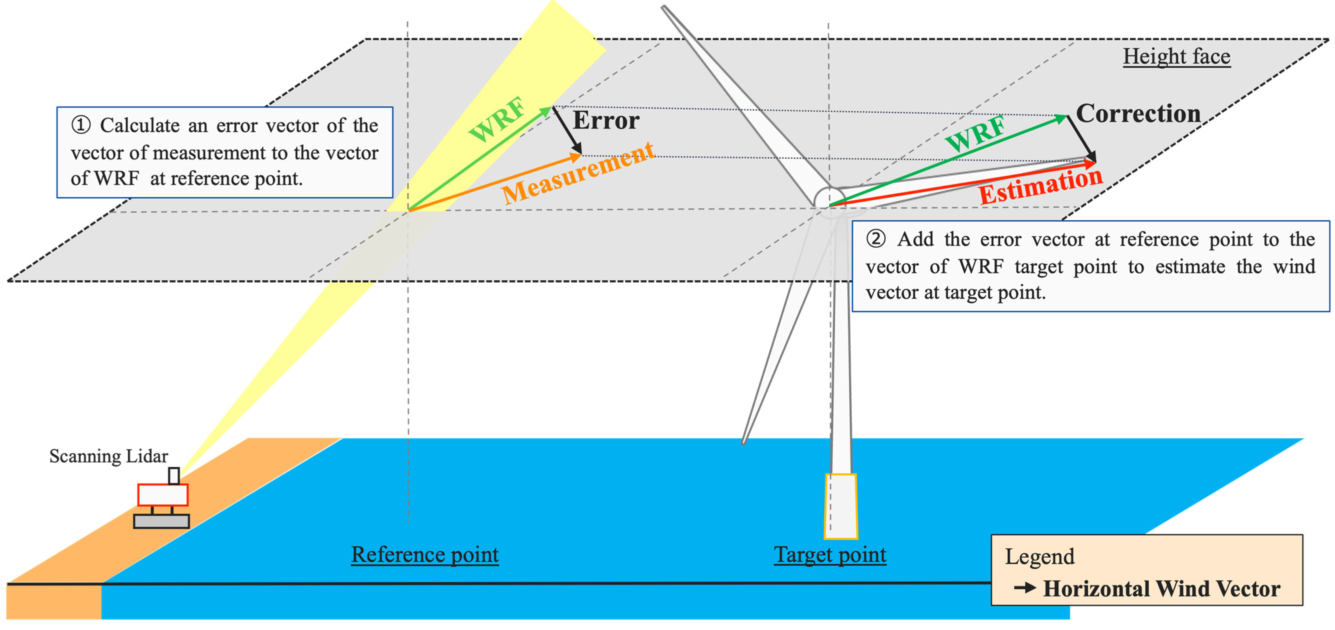
In principle, the correction coefficient $\alpha$ should depend on the correlation coefficient between the reference and target points (hereafter “reference–target correlation coefficient”); however, no empirical relationship has yet been established. Therefore, previous applications of the TC method, including our earlier study, have evaluated its accuracy with $\alpha$ fixed to unity. In Section 3, we derive empirical relationships for $\alpha$ based on the reference–target correlation coefficient and investigate how these formulations affect the estimation accuracy.

2.2.3. Direct Application of Time Series at a Reference Point (DA)

The third method is the direct application (DA) method, in which the measurement time series at the reference point are used directly as estimates at the target point without any correction or spatial extrapolation. Although DA is not used in practice, its accuracy relative to the WRF-based methods (CTRL and TC) provides a useful benchmark to assess the accuracy of spatial extrapolation using WRF.

2.3. Accuracy Indicators and Regression Statistics

This section describes the statistical indicators used to evaluate the estimation methods in this study.

First, following our previous study [30], the model error at time stamp $t_i$ is defined as

$$e\left(t_i\right)=P\left(t_i\right)-O\left(t_i\right)$$

(3)

where $P\left(t_i\right)$ and $O\left(t_i\right)$ are the estimated and measured values at time stamp $t_i\left(i=1,\dots ,n\right)$, respectively. For simplicity, in the following equations, we denote these quantities by $P_i=P\left(t_i\right)$, $O_i=O\left(t_i\right)$, and $e_i=e\left(t_i\right)$. Their sample means are denoted by $\bar{P}$ and $\bar{O}$, respectively.

The bias (mean error) is defined as the average of the errors over $n$ samples,

$$Bias={\displaystyle \frac{1}{n}}{\displaystyle \sum _{i=1}^n}{e}_i$$

(4)

and the relative bias is given by

$$Relative Bias \left[\%\right]={\displaystyle \frac{Bias}{\overline{O}}}\times 100$$

(5)

The linear (Pearson) correlation coefficient $R$ between the estimated and measured values is defined as

$$R={\displaystyle \frac{{\sum }_{i=1}^n\left(P_i-\overline{P}\right)\left(O_i-\overline{O}\right)}{\sqrt{{\sum }_{i=1}^n{\left(P_i-\overline{P}\right)}^2}\sqrt{{\sum }_{i=1}^n{\left(O_i-\overline{O}\right)}^2}}}$$

(6)

In addition, when constructing the empirical relationships in Section 3, we use a linear regression constrained to pass through the point $(1, 1)$ in the normalized space. The slope $a$ of this regression line and the coefficient of determination $R^2$ [34] are given by

$$y=1-a(1-x)$$

(7)

$$a={\displaystyle \frac{{\sum }_{i=1}^n{(x}_i-1\left)\right(y_i-1)}{{\sum }_{i=1}^n{{(x}_i-1)}^2}}$$

(8)

$$R^2=1-{\displaystyle \frac{{\sum }_{i=1}^n{\left(y_i-{\widehat{y}}_i\right)}^2}{{\sum }_{i=1}^n{\left(y_i-\overline{y}\right)}^2}}$$

(9)

where $x_i$ is the independent variable, $y_i$ is the dependent variable, ${\widehat{y}}_i$ is the regression estimate, and $\overline{y}$ is the mean value of $y_i$.

3. Characteristics and Extensions of the TC Method

In this section, Section 3.1 evaluates the estimation accuracy of the existing Temporal Correction methodology, while Section 3.2 presents the proposed extensions based on the results of Section 3.1.

3.1. Accuracy of the Existing TC Method

By comparing the estimation accuracy of the existing TC method with a fixed correction coefficient of α = 1 (hereafter TC-1) against that of CTRL and DA at Ishikari and Yuri-Honjo, this section investigates how the performance of TC depends on the reference–target correlation coefficient and explores a strategy for extending the TC method. This evaluation follows the validation framework adopted in our previous study, Maruo and Ohsawa [30].

Table 3 lists the combinations of reference points and their corresponding target points used for TC and DA. At Ishikari, only one height (142 m) was evaluated, whereas at Yuri-Honjo three heights (40, 100 and 160 m) were used. In all combinations, the reference and target points were at the same height. Among the combinations listed in Table 3, 48 combinations at Ishikari and 6 combinations at Yuri-Honjo (2 target points × 3 heights) for TC and DA involve unique reference–target combinations. In contrast, for CTRL, which does not utilize measurement data, validation was performed for all 15 target points.

Table 3. Combinations of reference and target points used for TC and DA. (a) Ishikari (single height: 142 m ASL); (b) Yuri-Honjo (three heights: 40, 100, and 160 m ASL). ✔ indicates a pair in which the reference and target are different points, and - indicates a pair in which the reference and target are the same point.

(a) Ishikari (142m)		Target Point
		N1	N2	N3	N4	N5	S1	S2	S3	S4
Reference Point	N1	-	✔	✔	✔	✔	✔	✔	✔	✔
	N2	✔	-	✔			✔	✔	✔
	N3	✔	✔	-			✔	✔	✔
	N4	✔			-	✔	✔			✔
	N5	✔			✔	-	✔			✔
	S1	✔	✔	✔	✔	✔	-	✔	✔	✔
	S2	✔	✔	✔			✔	-	✔
	S3	✔	✔	✔			✔	✔	-
	S4	✔			✔	✔	✔			-
(b) Yuri-Honjo			Target Point
			NSL				SSL
			40 m		100 m	160 m	40 m		100 m	160 m
Reference Point	NSL	40 m	-				✔
		100 m			-				✔
		160 m				-				✔
	SSL	40 m	✔				-
		100 m			✔				-
		160 m				✔				-

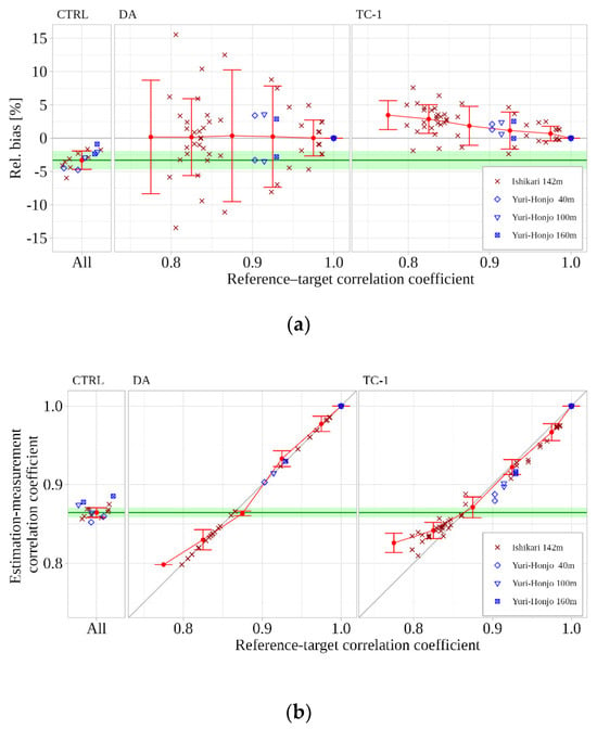
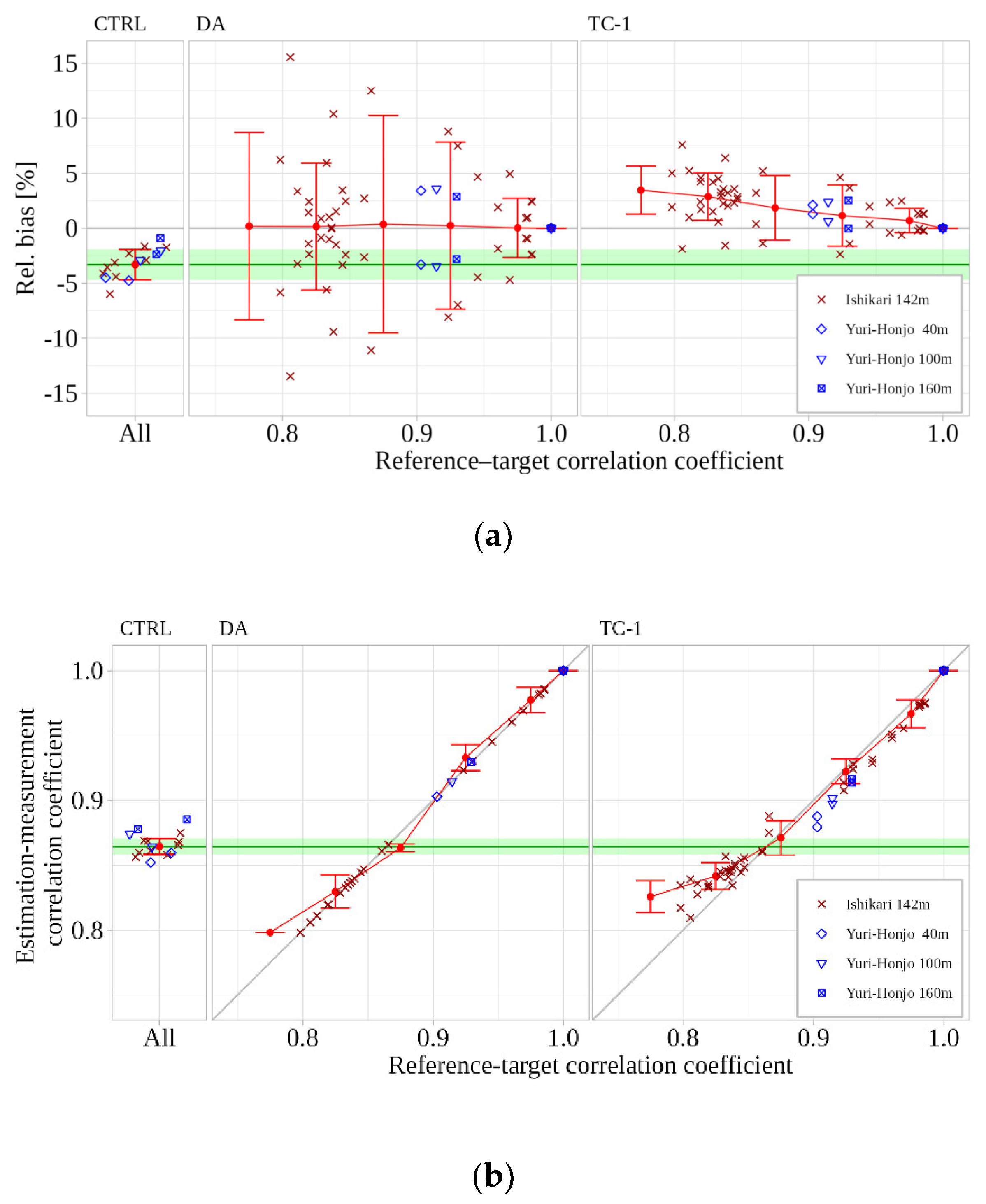
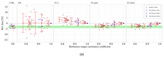
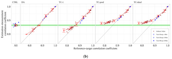
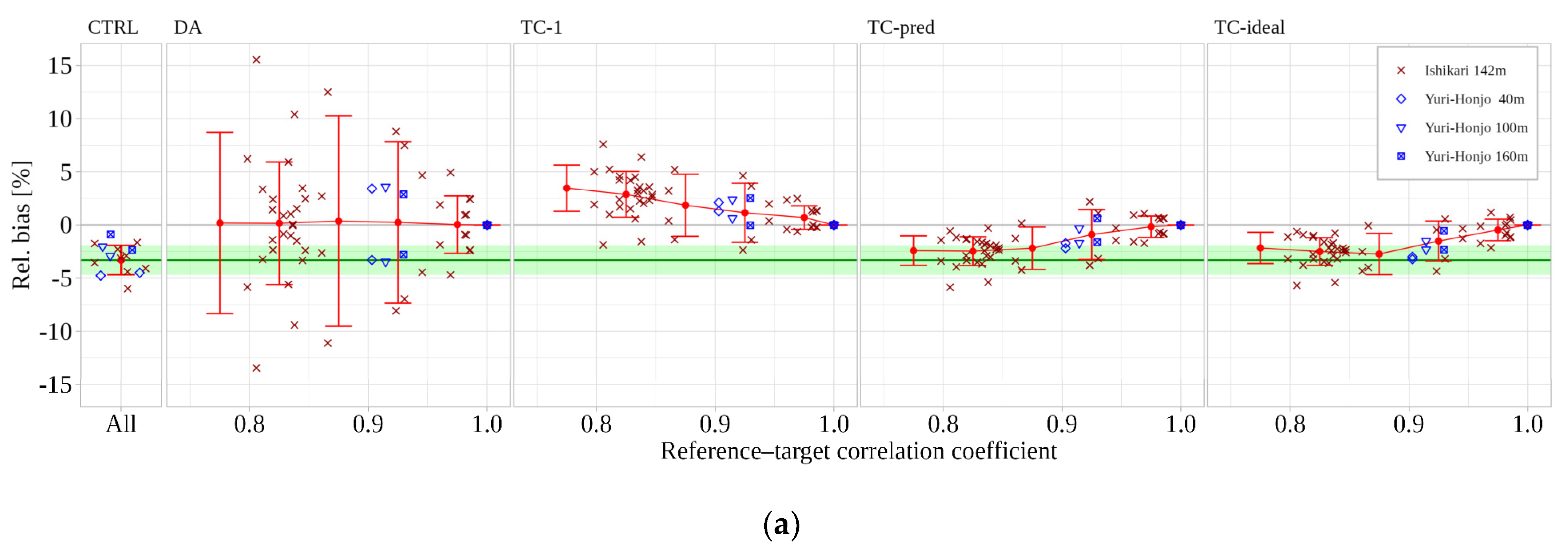
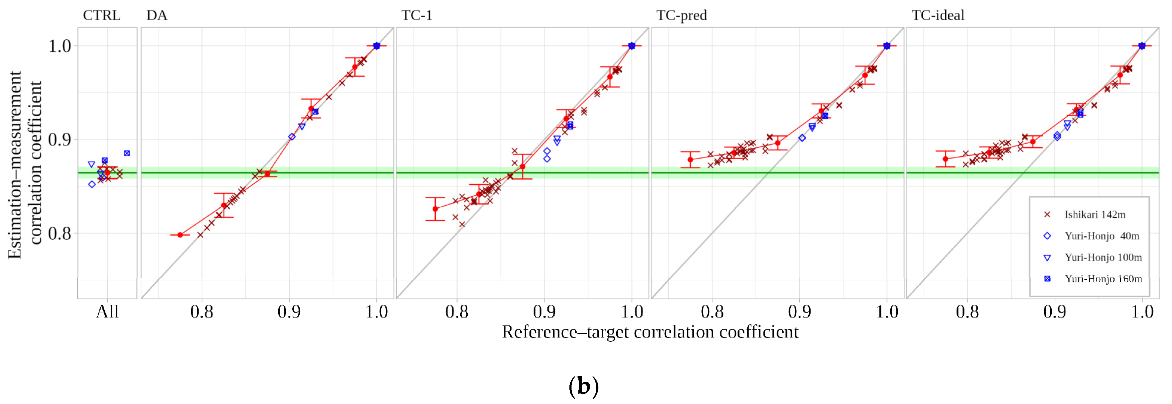
Because the estimation accuracy is expected to be closely related to the reference–target correlation, we examined the relationship between the reference–target correlation coefficient and the wind-speed estimation accuracy at target points at Ishikari and Yuri-Honjo. Figure 4 shows scatter plots of the accuracy indicators (relative bias or estimation–measurement correlation coefficient) versus the reference–target correlation coefficient for each method. The results are compared among CTRL, DA, and TC-1 ($\alpha = 1$). The reference–target correlation coefficients are grouped into bins of 0.70–0.75, …, 0.95–1.00, and exactly 1.00. Red symbols indicate the bin-averaged accuracy at Ishikari (relative bias or estimation–measurement correlation coefficient), red error bars indicate mean ± 1 standard deviation of accuracy indicators within each bin, and the green shaded area shows the corresponding range for CTRL at Ishikari. The samples from Yuri-Honjo at 40, 100, and 160 m are plotted in blue to assess whether the tendencies observed at Ishikari are site-independent; these samples are not included in the calculation of the bin-averaged values and error bars. Because the accuracy indicators of CTRL are independent of the reference–target correlation, their values are plotted at a fixed horizontal position. For DA, the estimation–measurement correlation coefficient follows the 1:1 relationship by construction.

Figure 4. Dependence of wind-speed estimation accuracy on the reference–target correlation for the three methods CTRL, DA, and TC-1: (a) relative bias and (b) estimation–measurement correlation coefficient.

At Ishikari (Figure 4a), the relative bias of CTRL ranged from −6.0% to −1.7%, indicating that WRF underestimated the mean wind speed at all points. In bins with reference–target correlation coefficients below 0.95, DA showed a relatively large spread of bias, indicating non-negligible differences in mean wind speed between the reference and target points. This suggests that, under lower-correlation conditions, the DA assumption of identical wind conditions between the reference and target points is not appropriate, and that accounting for spatial differences between them becomes important. In contrast to CTRL, TC-1 exhibited mostly positive bias values, with the positive deviation becoming more pronounced as the reference–target correlation coefficient decreased. The binned-averaged mean (red points) and its standard deviation range (the red error bars) for TC-1 also deviated from 0 as the reference–target correlation coefficient decreased, becoming comparable to those of CTRL in the 0.80–0.85 bin.

Figure 4b presents the relationship between the reference–target correlation coefficient and the estimation–measurement correlation coefficient. For DA, these two quantities are mathematically identical, because the estimated wind speed at the target point is given directly by the measured wind speed at the reference point. Therefore, the estimation–measurement correlation coefficient for DA lies on the 1:1 line $\left(y=x\right)$. The estimation–measurement correlation coefficient of CTRL at Ishikari ranged from 0.85 to 0.88. When the reference–target correlation coefficient was higher than 0.90, TC-1 closely followed the 1:1 line and clearly outperformed CTRL in this range. In contrast, when the reference–target correlation coefficient was below 0.85, TC-1 yielded lower estimation–measurement correlation coefficients than CTRL.

At Yuri-Honjo, both the relative bias and the estimation–measurement correlation coefficient for CTRL and TC-1 exhibited tendencies similar to those at Ishikari, although most samples were limited to the reference–target correlation coefficient range of 0.90–0.95.

In the following, improvement in accuracy relative to CTRL is regarded as evidence of the effectiveness of TC. From Figure 4a, TC-1 is clearly effective in bias correction when the reference–target correlation coefficient exceeds 0.90, while in the range 0.75–0.85 it performs comparably to CTRL with opposite signs. In terms of the estimation–measurement correlation coefficient, TC-1 is also effective above 0.90, comparable to CTRL in the range 0.85–0.90, but ineffective below 0.85. For both accuracy indicators, a clear relationship is observed between the reference–target correlation and estimation accuracy. These diagnostic results indicate that the correction coefficient α should decrease from unity as the reference–target correlation coefficient decreases.

3.2. Methodological Extensions

3.2.1. Formulation of an Extended TC Method

As indicated by the diagnostic results in Section 3.1, $\alpha$ should decrease from unity as the reference–target correlation coefficient decreases. Accordingly, in the extended method, $\alpha$ is expressed as a function of the reference–target correlation coefficient $r$:

$$\alpha =\alpha \left(r\right)$$

(10)

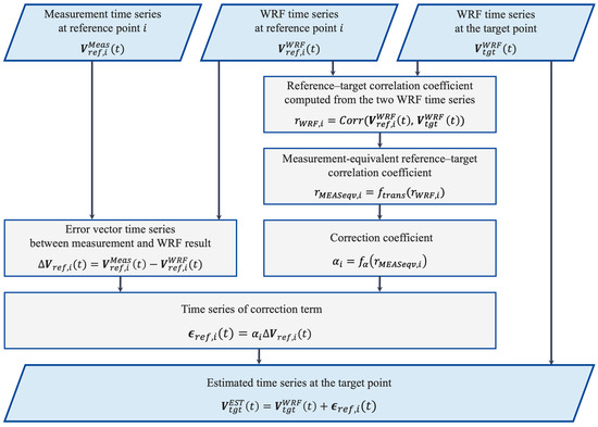
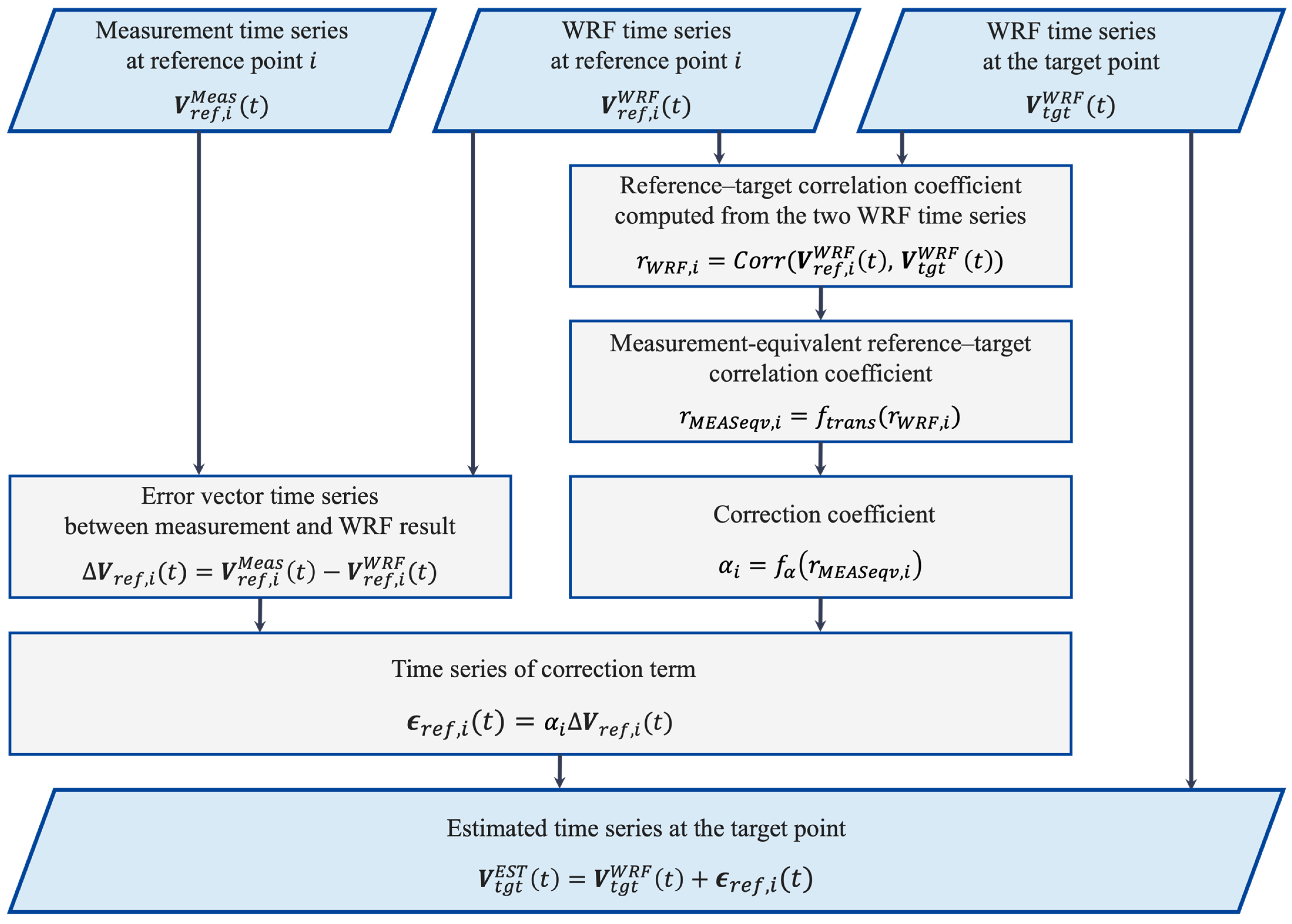
In practical applications, however, the reference–target correlation coefficient based on measurement data cannot be obtained because measurement data at the target point are not available. To enable this practical application, the extended method introduces two empirical relationships. First, the reference–target correlation coefficient estimated from WRF, $r_{WRF,i}$, is transformed into a measurement-equivalent correlation, $r_{MEASeqv,i}$ through a correlation-conversion function $f_{trans}$. Second, the correction coefficient $\alpha$ is determined from the transformed correlation, $r_{\mathrm{M}\mathrm{E}\mathrm{A}\mathrm{S}\mathrm{e}\mathrm{q}\mathrm{v},i}$ through an alpha-prediction function $f_{\alpha }$. The quantities and functions used in this formulation are defined in Table 4, and the overall procedure for wind estimation using these relationships is shown in Figure 5.

Table 4. Definitions of quantities and functions used in the formulation.

Symbols	Explanations
$r_{WRF,i}$	Correlation coefficient between reference point i and the target point (reference–target correlation coefficient), estimated from WRF
$r_{MEAS,i}$	Correlation coefficient between reference point i and the target point (reference–target correlation coefficient), derived from measurement data (not available in practice)
$f_{trans}$	Correlation-conversion function; an empirical regression function that converts $r_{WRF,i}$ to $r_{MEASeqv,i}$
$r_{MEASeqv,i}=f_{trans}\left(r_{WRF,i}\right)$	Measurement-equivalent reference–target correlation coefficient, estimated from $r_{WRF,i}$ using the empirical transformation $f_{trans}$
$f_{\alpha }$	Alpha-prediction function; an empirical regression function that predicts ${\alpha }_i$ from $r_{\mathrm{M}\mathrm{E}\mathrm{A}\mathrm{S},i}$
${\alpha }_i=f_{\alpha }\left(r_{MEASeqv,i}\right)=f_{\alpha }\left(f_{trans}\left(r_{WRF,i}\right)\right)$	Correction coefficient for reference point i in the extended TC method

Figure 5. Flowchart of the TC-pred procedure for single-reference-point wind estimation.

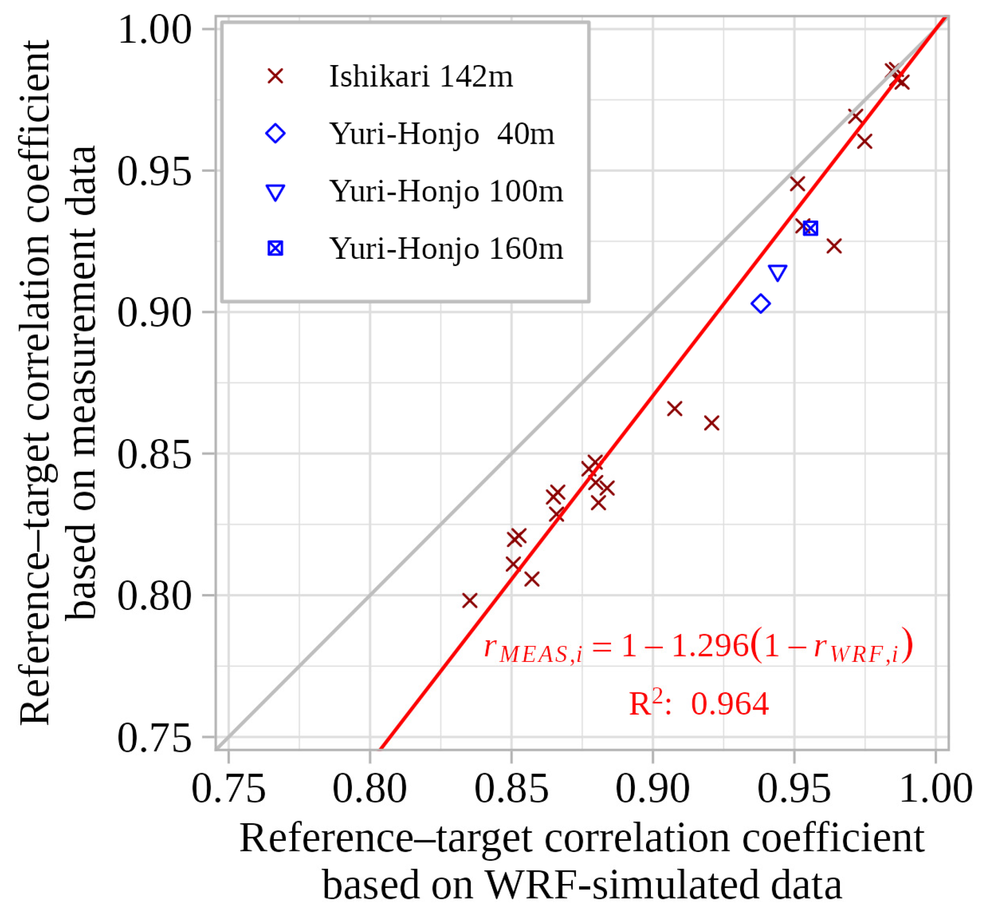
First, the correlation-conversion function $f_{trans}$ was derived by examining the relationship between $r_{WRF,i}$ and $r_{MEAS,i}$. The results are shown in Figure 6. In this figure, the red markers and the regression line constrained to pass through $(1, 1)$ represent the results from Ishikari, while the blue markers represent those from Yuri-Honjo and are used to assess whether the tendency observed at Ishikari is site-independent. The plot shows that $r_{WRF,i}$ tends to be higher than $r_{MEAS,i}$; however, a strong linear relationship is evident between the two (the coefficient of determination is 0.96). Moreover, the samples from Yuri-Honjo lie close to the regression line derived from the Ishikari samples, suggesting that this line captures a general relationship between $r_{WRF,i}$ and $r_{MEAS,i}$. Accordingly, this study adopts the following regression line as the correlation-conversion function $f_{\mathrm{t}\mathrm{r}\mathrm{a}\mathrm{n}\mathrm{s}}$:

Figure 6. Empirical relationship between WRF-derived and measurement-derived reference–target correlation ($r_{\mathrm{W}\mathrm{R}\mathrm{F},i}$ and $r_{\mathrm{M}\mathrm{E}\mathrm{A}\mathrm{S},i}$). Reference–target correlation coefficients estimated from WRF time series are compared with those derived from measurements. The regression line (constrained to pass through $\left(\mathrm{1,1}\right)$) provides the correlation-conversion function used to obtain measurement-equivalent correlations from WRF-only information. Ishikari samples are shown in red, and Yuri-Honjo samples (40, 100, and 160 m) are shown in blue for cross-site assessment.

Figure 6. Empirical relationship between WRF-derived and measurement-derived reference–target correlation ($r_{\mathrm{W}\mathrm{R}\mathrm{F},i}$ and $r_{\mathrm{M}\mathrm{E}\mathrm{A}\mathrm{S},i}$). Reference–target correlation coefficients estimated from WRF time series are compared with those derived from measurements. The regression line (constrained to pass through $\left(\mathrm{1,1}\right)$) provides the correlation-conversion function used to obtain measurement-equivalent correlations from WRF-only information. Ishikari samples are shown in red, and Yuri-Honjo samples (40, 100, and 160 m) are shown in blue for cross-site assessment.

$$r_{MEASeqv,i}=1-1.30 (1-r_{WRF,i})$$

(11)

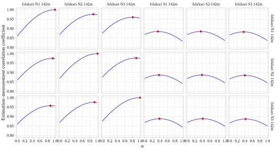
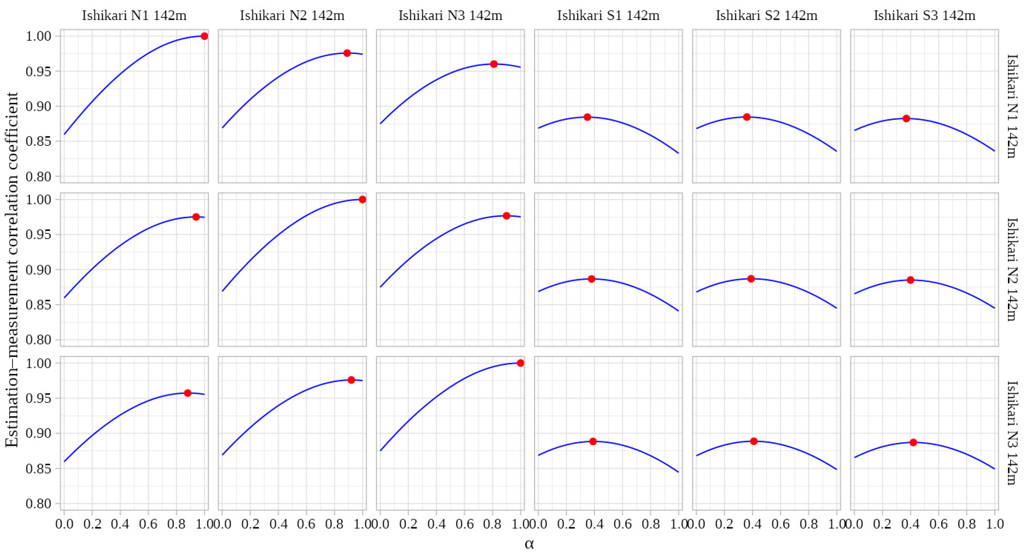
Next, the alpha-prediction function $f_{\alpha }$ was derived by examining the relationship between $r_{MEAS,i}$ and the value of $\alpha$ that maximizes the estimation–measurement correlation coefficient. For each pair of reference and target points listed in Table 3, $\alpha$ was varied from 0.00 to 1.00 in increments of 0.01, and the corresponding estimation–measurement correlation coefficient of wind speeds at the target point was computed. The value of $\alpha$ that maximized this correlation coefficient was then identified for each reference–target pair. The results are shown in Figure 7. In each subplot, the horizontal axis represents $\alpha$ and the vertical axis represents the estimation–measurement correlation coefficient. The blue curve shows how this correlation coefficient changes with $\alpha$, and the red marker indicates the value of $\alpha$ at which the correlation coefficient attains its maximum. The subplots are arranged such that reference points vary horizontally and target points vary vertically. Figure 7 shows that, when the reference and target points coincide, the value of $\alpha$ that maximizes the estimation–measurement correlation coefficient is 1 in principle, and that this value tends to decrease as the correlation between them decreases.

Figure 7. Variation in the estimation–measurement correlation coefficient with the correction coefficient α for selected reference–target pairs in Ishikari Group A at 142 m. Blue curves show the response to α, and red markers indicate the maximum point for each pair.

In Figure 8, the values of $\alpha$ that maximized the estimation–measurement correlation coefficient in Figure 7 were then plotted against the corresponding measurement-based reference–target correlation coefficients, $r_{MEAS,i}$. The horizontal axis represents the reference–target correlation coefficient (based on measurements), and the vertical axis represents the corresponding values of α that maximize the estimation–measurement correlation coefficient. The red markers and the regression line represent the results from Ishikari, whereas the blue markers represent those from Yuri-Honjo and are used to assess whether the tendency observed at Ishikari is site-independent. The Ishikari results indicate a strong linear relationship (the coefficient of determination is 0.96) between $r_{MEAS,i}$ and ${\alpha }_i$, which can be expressed as

Figure 8. Empirical relationship between reference–target correlation coefficient ($r_{\mathrm{M}\mathrm{E}\mathrm{A}\mathrm{S},i}$.) and the correction coefficient identified in Figure 7 (${\alpha }_{\mathrm{i}}$). The ${\alpha }_{\mathrm{i}}$ values are plotted against the corresponding reference–target correlation (based on measurements). The regression line (constrained to pass through $\left(\mathrm{1,1}\right)$) provides the alpha-prediction function to predict ${\alpha }_i$ from $r_{\mathrm{M}\mathrm{E}\mathrm{A}\mathrm{S},i}$. Red symbols denote Ishikari samples used to fit the regression, and Yuri-Honjo samples at multiple heights are shown in blue for cross-site assessment.

Figure 8. Empirical relationship between reference–target correlation coefficient ($r_{\mathrm{M}\mathrm{E}\mathrm{A}\mathrm{S},i}$.) and the correction coefficient identified in Figure 7 (${\alpha }_{\mathrm{i}}$). The ${\alpha }_{\mathrm{i}}$ values are plotted against the corresponding reference–target correlation (based on measurements). The regression line (constrained to pass through $\left(\mathrm{1,1}\right)$) provides the alpha-prediction function to predict ${\alpha }_i$ from $r_{\mathrm{M}\mathrm{E}\mathrm{A}\mathrm{S},i}$. Red symbols denote Ishikari samples used to fit the regression, and Yuri-Honjo samples at multiple heights are shown in blue for cross-site assessment.

$${\alpha }_i=1-3.53 (1-\hspace{0.17em}{r}_{MEAS,i}) (\alpha \ge 0)$$

(12)

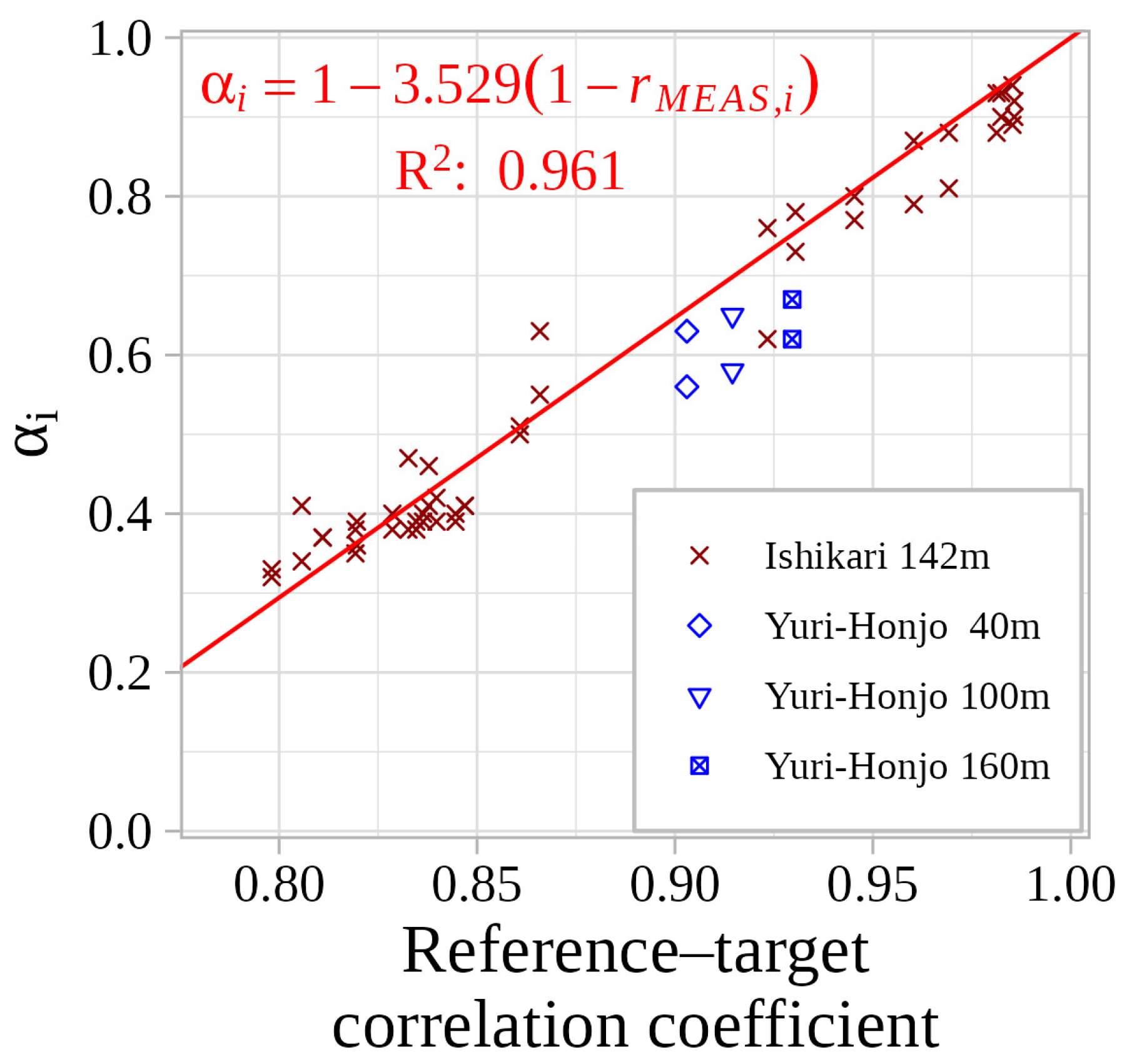
Furthermore, the samples from Yuri-Honjo lie close to the regression line derived from the Ishikari samples, suggesting that this relationship captures a consistent underlying characteristic. Accordingly, this study adopts the above regression line as the empirical function $f_{\alpha }$.

3.2.2. Accuracy Evaluation of the Extended TC Method

This subsection evaluates the effectiveness of the extended TC method (TC-pred) using the correction coefficient ${\alpha }_i$ predicted through the two empirical functions proposed in Section 3.2.1 for the single-reference case. The following methods are compared: CTRL, DA, TC with a fixed correction coefficient of $\alpha =1$ (TC-1), an idealized method (TC-ideal) in which the value of $\alpha$ that maximizes the estimation–measurement correlation coefficient is directly determined for each reference–target pair using the target-point measurement data, and the proposed method (TC-pred), in which ${\alpha }_i$ is predicted only from the WRF-derived reference–target correlation coefficient through the two empirical functions $f_{trans}$ and $f_{\alpha }$. The results are summarized in Figure 9. As in the previous section, the red markers and error bars represent the samples and statistics from Ishikari, while the blue markers show the samples from Yuri-Honjo.

Figure 9. Dependence of wind-speed estimation accuracy on the reference–target correlation for the five methods CTRL, DA, TC-1, TC-pred and TC-ideal: (a) relative bias and (b) estimation–measurement correlation coefficient.

Regarding relative bias, TC-1 exhibits a general tendency to overestimate the mean wind speed, whereas TC-pred shows an underestimation tendency. This behavior is consistent with the fact that the predicted α in TC-pred takes values between 0 and 1, yielding a bias that lies between that of CTRL (negative bias) and TC-1 (positive bias). When comparing CTRL and TC-pred, TC-pred exhibits zero bias when the reference–target correlation coefficient is 1, and even in the 0.75–0.80 bin, the magnitude of the bias for TC-pred tends to be smaller than that for CTRL.

For the estimation–measurement correlation coefficient, TC-1 and TC-pred produce almost identical values in the 0.90–0.95 and 0.95–1.00 bins. However, for reference–target correlation coefficients below 0.90, TC-pred clearly outperforms TC-1. Furthermore, even in the 0.75–0.80 bin, the estimation–measurement correlation coefficient for TC-pred tends to be slightly larger than that for CTRL. This indicates that the predicted correction coefficient enables TC to maintain higher correlation with the measurements even when the reference–target correlation coefficient is relatively low.

Additionally, although the available range of reference–target correlation coefficients at Yuri-Honjo is limited, the tendencies observed there are consistent with those obtained at Ishikari for both relative bias and estimation–measurement correlation coefficient.

Taken together, these results show that TC-pred, using smaller values of α than TC-1, achieves better accuracy than CTRL over a wider range of reference–target correlation coefficients, i.e., it provides effective correction over a broader spatial range. Furthermore, a comparison between TC-ideal and TC-pred reveals that their relative bias and estimation–measurement correlation coefficient are almost indistinguishable, indicating that the prediction error in ${\alpha }_i$ introduced by the two empirical functions does not degrade wind estimation accuracy.

4. Extensions of the TC Method for Multiple Reference Points

4.1. Weighting Strategy for Multiple Reference Points

This subsection describes the weighting strategy used to extend TC-pred to the case with multiple reference points.

In the single-reference case, the correction term is written as

$${\mathit{ϵ}}_{ref}(x_n,y_n,z_n,t)=\alpha \hspace{0.17em}\mathit{\Delta }{\mathit{V}}_{ref}(x_n,y_n,z_n,t).$$

(13)

For simplicity, the explicit dependence on $(x_n,y_n,z_n,t)$ is omitted hereafter. When multiple reference points are used, the contributions from the different reference points cannot be simply added without adjustment, because the error vectors at the reference points are not mutually independent and may contain overlapping correction components. Such a treatment would amount to multiple counting the correction and would tend to overestimate its magnitude. Therefore, a weighting coefficient $w_i$ is introduced to appropriately distribute the correction among the reference points, and the formulation is then generalized as

$${\mathit{ϵ}}_{ref}={\displaystyle \sum _{i=1}^n}{\alpha }_i{w}_i\hspace{0.17em}\mathsf{\Delta }{\mathit{V}}_i.$$

(14)

The weighting coefficient $w_i$ is defined as

$$w_i={\displaystyle \frac{{\prod }_{j\ne i}{l}_j}{{\displaystyle {\sum }_{k=1}^n}{\prod }_{j\ne k}{l}_j}}$$

(15)

where $\left.l_i\in [0,\mathrm{\infty }\right)$ is a nonnegative index characterizing the relationship between reference point $i$ and the target point. Here, $l_i=0$ indicates that reference point $i$ coincides with the target point, and larger values indicate a weaker relationship. By construction, $w_i\ge 0$ and ${\sum }_{i=1}^n{w}_i=1$. Thus, the set of weights $w_i$ can be interpreted as the relative contributions of the reference points to the total correction.

Although Equation (15) is written in a product form, for $l_i>0$ it is algebraically equivalent to

$$w_i={\displaystyle \frac{l_i^{-1}}{{\displaystyle {\sum }_{k=1}^n}{l}_k^{-1}}}.$$

(16)

Thus, the weighting is essentially a normalized inverse-$l_i$ weighting, in which reference points with smaller $l_i$ are assigned larger weights. The product form is retained because it naturally avoids division by zero when $l_i=0$. When $l_i=0$, Equation (15) gives $w_i=1$ and $w_j=0$ for $j\ne i$. This means that, when the target point coincides with reference point $i$, the estimated value exactly reproduces the reference value at that point. Such a self-consistency property is natural and desirable for a correction model.

In this study, $l_i$ is not given directly by geometric distance but is derived from the correction coefficient $\left.{\alpha }_i\in (\mathrm{0,1}\right]$ as

$$l_i={\displaystyle \frac{1-{\alpha }_i}{{\alpha }_i}}$$

(17)

where larger ${\alpha }_i$ indicates a stronger relationship between reference point $i$ and the target point; reference points with ${\alpha }_i=0$ are not used in the estimation. Since $l_i$ decreases monotonically with increasing ${\alpha }_i$, reference points with larger ${\alpha }_i$ are assigned larger weights. Substituting Equation (17) into Equation (16) gives

$$w_i={\displaystyle \frac{{\alpha }_i/(1-{\alpha }_i)}{{\displaystyle {\sum }_{k=1}^n}{\alpha }_k/(1-{\alpha }_k)}}$$

(18)

showing that the weighting is determined by the relative values of ${\alpha }_i$ without introducing any additional tuning parameter. The key feature of this formulation is that $l_i$ is defined from the correction coefficient ${\alpha }_i$ rather than from the geometric distance. The rationale for this choice is discussed in Section 5.

4.2. Case of Two and Three Reference Points

In the case using two reference points, the weighting coefficients $w_1$ and $w_2$, the weighted correction coefficients ${\alpha }_1{w}_1$ and ${\alpha }_2{w}_2$, and their sum ${\alpha }_{sum}$ can be written as functions of ${\alpha }_1$ and ${\alpha }_2$.

The corresponding $l_i$ values are

$$l_1={\displaystyle \frac{1-{\alpha }_1}{{\alpha }_1}}$$

(19)

$$l_2={\displaystyle \frac{1-{\alpha }_2}{{\alpha }_2}}$$

(20)

Using the definition of the weighting coefficient $w_i$, we obtain

$$w_1={\displaystyle \frac{l_2}{l_1+l_2}}={\displaystyle \frac{\frac{1-{\alpha }_2}{{\alpha }_2}}{\frac{1-{\alpha }_1}{{\alpha }_1}+\frac{1-{\alpha }_2}{{\alpha }_2}}}$$

(21)

$$w_2={\displaystyle \frac{l_1}{l_1+l_2}}={\displaystyle \frac{\frac{1-{\alpha }_1}{{\alpha }_1}}{\frac{1-{\alpha }_1}{{\alpha }_1}+\frac{1-{\alpha }_2}{{\alpha }_2}}}$$

(22)

Although ${\alpha }_{\mathrm{s}\mathrm{u}\mathrm{m}}={\alpha }_1{w}_1+{\alpha }_2{w}_2$ does not appear explicitly in the final correction formula, it is introduced here as an auxiliary indicator of the overall level of the weighted correction coefficients. ${\alpha }_{sum}$ is then

$${\alpha }_{sum}={\alpha }_1{w}_1+{\alpha }_2{w}_2={\displaystyle \frac{{\alpha }_1^2(1-{\alpha }_2)+{\alpha }_2^2(1-{\alpha }_1)}{{\alpha }_1(1-{\alpha }_2)+{\alpha }_2(1-{\alpha }_1)}}$$

(23)

When $0<{\alpha }_i<1$,

$${\alpha }_{sum}={\displaystyle \frac{\frac{{\alpha }_1^2}{1-{\alpha }_1}+\frac{{\alpha }_2^2}{1-{\alpha }_2}}{\frac{{\alpha }_1}{1-{\alpha }_1}+\frac{{\alpha }_2}{1-{\alpha }_2}}}$$

(24)

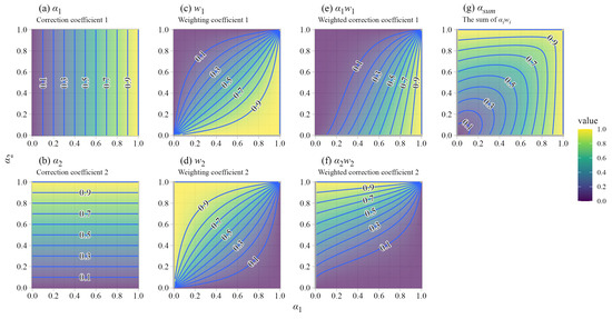
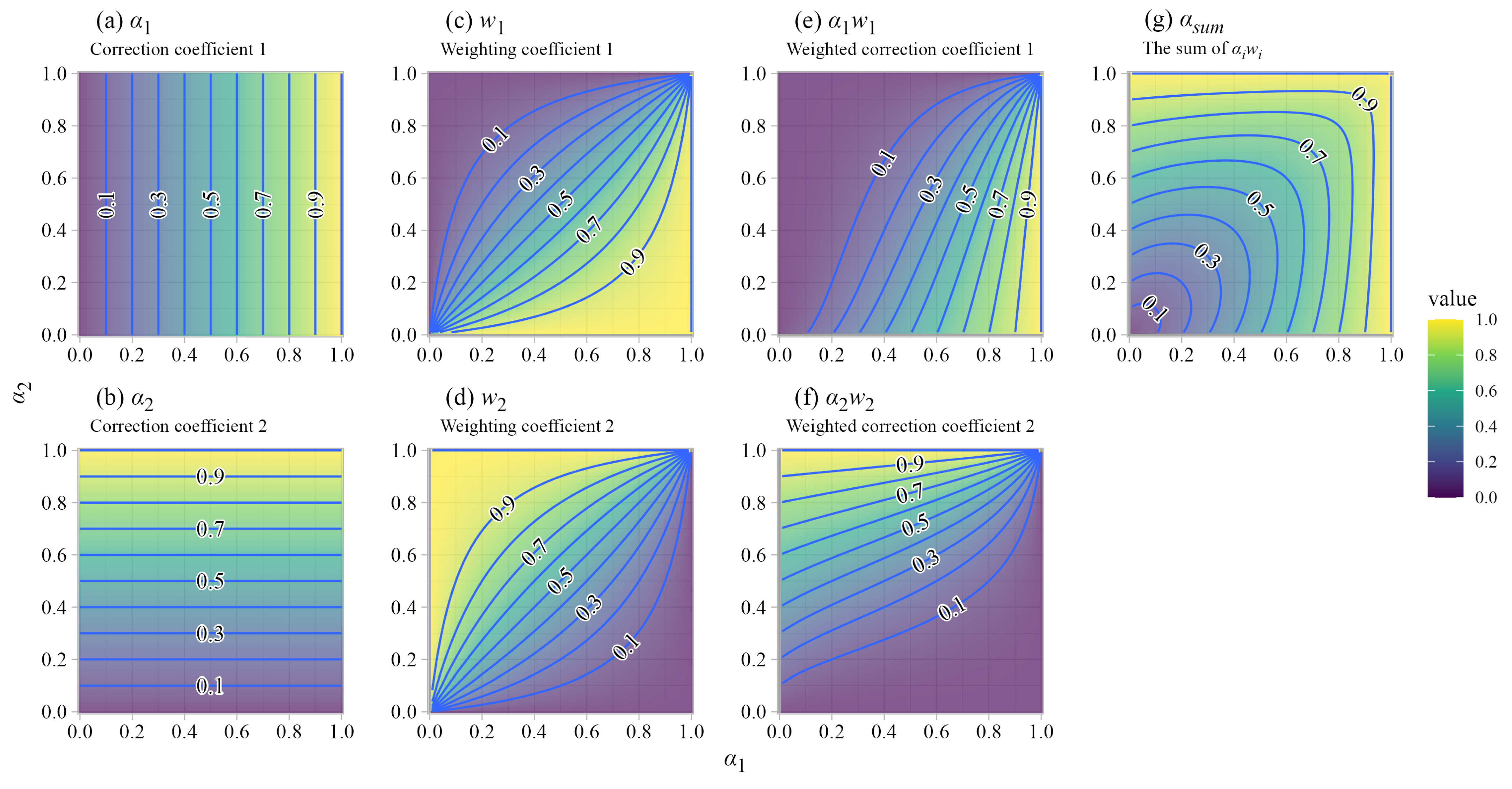
Figure 10 shows the dependence of $w_1$, $w_2$, ${\alpha }_1{w}_1$, ${\alpha }_2{w}_2$, and ${\alpha }_{\mathrm{s}\mathrm{u}\mathrm{m}}$ on ${\alpha }_1$ and ${\alpha }_2$. Their values vary smoothly in response to the relative values of ${\alpha }_1$ and ${\alpha }_2$.

Figure 10. Behavior of spatial weights and contribution coefficients for the two-reference-point case. Contour plots illustrate how the weighting coefficient ($w_1$, $w_2$), weighted correction coefficients (${\alpha }_1{w}_1$, ${\alpha }_2{w}_2$), and their sum (${\alpha }_{sum}$) vary as functions of the correction coefficients (${\alpha }_1$, ${\alpha }_2$).

Regarding ${\alpha }_{sum}$, since $w_1,w_2\ge 0$ and $w_1+w_2=1$, ${\alpha }_{\mathrm{s}\mathrm{u}\mathrm{m}}$ satisfies

$$0\le \mathrm{m}\mathrm{i}\mathrm{n}({\alpha }_1,{\alpha }_2)\le {\alpha }_{\mathrm{s}\mathrm{u}\mathrm{m}}\le \mathrm{m}\mathrm{a}\mathrm{x}({\alpha }_1,{\alpha }_2)\le 1.$$

(25)

Thus, ${\alpha }_{\mathrm{s}\mathrm{u}\mathrm{m}}$ lies between ${\alpha }_1$ and ${\alpha }_2$. Figure 10 also shows that the weighting keeps ${\alpha }_{\mathrm{s}\mathrm{u}\mathrm{m}}$ close to that of the reference point with the larger $\alpha$. This indicates that the relationship between ${\alpha }_{sum}$ and $r$ remains broadly consistent with the relationship between ${\alpha }_i$ and $r$ described in Section 3.

Note that, in the case using three reference points, ${\alpha }_{sum}$ is

$${\alpha }_{sum}={\alpha }_1{w}_1+{\alpha }_2{w}_2+{\alpha }_3{w}_3={\displaystyle \frac{{\alpha }_1^2\left(1-{\alpha }_2\right)\left(1-{\alpha }_3\right)+{\alpha }_2^2\left(1-{\alpha }_1\right)\left(1-{\alpha }_3\right)+{\alpha }_3^2\left(1-{\alpha }_1\right)\left(1-{\alpha }_2\right)}{{\alpha }_1\left(1-{\alpha }_2\right)\left(1-{\alpha }_3\right)+{\alpha }_2\left(1-{\alpha }_1\right)\left(1-{\alpha }_3\right)+{\alpha }_3\left(1-{\alpha }_1\right)\left(1-{\alpha }_2\right)}}.$$

(26)

When $0<{\alpha }_i<1$,

$${\alpha }_{sum}={\displaystyle \frac{\frac{{\alpha }_1^2}{1-{\alpha }_1}+\frac{{\alpha }_2^2}{1-{\alpha }_2}+\frac{{\alpha }_3^2}{1-{\alpha }_3}}{\frac{{\alpha }_1}{1-{\alpha }_1}+\frac{{\alpha }_2}{1-{\alpha }_2}+\frac{{\alpha }_3}{1-{\alpha }_3}}}.$$

(27)

4.3. Accuracy Evaluation with Multiple Reference Points

This subsection uses the measurement data at Ishikari to evaluate the estimation accuracy changes when multiple reference points are used. The combinations of reference and target points considered in the validation are listed in Table 5. In the table, R indicates reference points, whereas T indicates target points that are different from the reference points. Entries marked as T* denote duplicated target entries included only to enable direct comparison between the single- and two-reference-point configurations. The single-reference configurations are identical to those examined in Section 3, and, similarly, datasets of estimated time series at the target points were constructed for each two-reference and three-reference-point configuration to compare their accuracy using relative bias and estimation–measurement correlation coefficient. The CTRL method, which uses no reference-point measurements, is treated as the zero-reference case. The Yuri-Honjo samples were not included in this analysis because only two measurement points were available, which does not allow multiple-reference-point configurations.

Table 5. Combinations of reference and target points at Ishikari for multiple-reference-point validation in Section 4: (a) case using a single reference point; (b) case using two reference points; and (c) case using three reference points.

(a) # of reference points: 1
No	Group	N1	N2	N3	N4	N5	S1	S2	S3	S4	# of target points
1	A	R	T	T			T	T	T		5
2		T	R	T			T	T	T		5
3		T	T	R			T	T	T		5
4		T	T	T			R	T	T		5
5		T	T	T			T	R	T		5
6		T	T	T			T	T	R		5
7	B	R			T	T	T*			T	3
8		T			R	T	T			T	4
9		T			T	R	T			T	4
10		T*			T	T	R			T	3
11		T			T	T	T			R	4
				Sample size excludes reference points							48
(b) # of reference points: 2
No	Group	N1	N2	N3	N4	N5	S1	S2	S3	S4	# of target points
1	A	R	R	T			T	T	T		4
2		R	T	R			T	T	T		4
3		R	T	T			R	T	T		4
4		R	T	T			T	R	T		4
5		R	T	T			T	T	R		4
6		T	R	R			T	T	T		4
7		T	R	T			R	T	T		4
8		T	R	T			T	R	T		4
9		T	R	T			T	T	R		4
10		T	T	R			R	T	T		4
11		T	T	R			T	R	T		4
12		T	T	R			T	T	R		4
13		T	T	T			R	R	T		4
14		T	T	T			R	T	R		4
15		T	T	T			T	R	R		4
16	B	R			R	T	T			T	3
17		R			T	R	T			T	3
18		R			T	T	R			T	3
19		R			T	T	T			R	3
20		T			R	R	T			T	3
21		T			R	T	R			T	3
22		T			R	T	T			R	3
23		T			T	R	R			T	3
24		T			T	R	T			R	3
25		T			T	T	R			R	3
				Sample size excludes reference points							90
(c) # of reference points: 3
No	Group	N1	N2	N3	N4	N5	S1	S2	S3	S4	# of target points
1	A	R	R	R			T	T	T		3
2		R	R	T			R	T	T		3
3		R	R	T			T	R	T		3
4		R	R	T			T	T	R		3
5		R	T	R			R	T	T		3
6		R	T	R			T	R	T		3
7		R	T	R			T	T	R		3
8		R	T	T			R	R	T		3
9		R	T	T			R	T	R		3
10		R	T	T			T	R	R		3
11		T	R	R			R	T	T		3
12		T	R	R			T	R	T		3
13		T	R	R			T	T	R		3
14		T	R	T			R	R	T		3
15		T	R	T			R	T	R		3
16		T	R	T			T	R	R		3
17		T	T	R			R	R	T		3
18		T	T	R			R	T	R		3
19		T	T	R			T	R	R		3
20		T	T	T			R	R	R		3
21	B	R			R	R	T			T	2
22		R			R	T	R			T	2
23		R			R	T	T			R	2
24		R			T	R	R			T	2
25		R			T	R	T			R	2
26		R			T	T	R			R	2
27		T			R	R	R			T	2
28		T			R	R	T			R	2
29		T			R	T	R			R	2
30		T			T	R	R			R	2
				Sample size excludes reference points							80

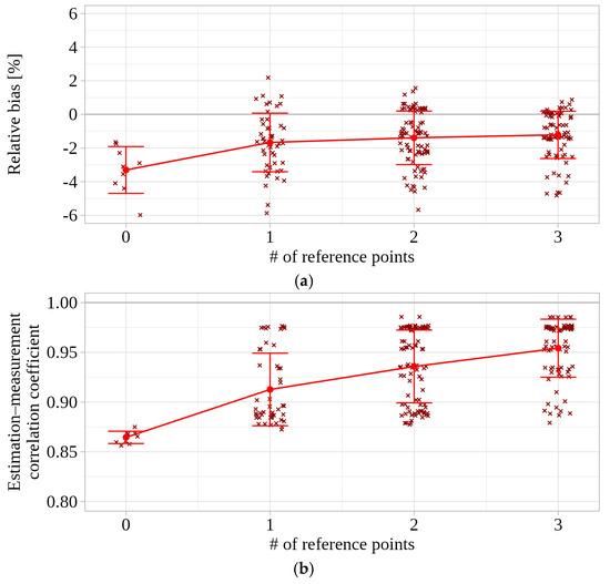
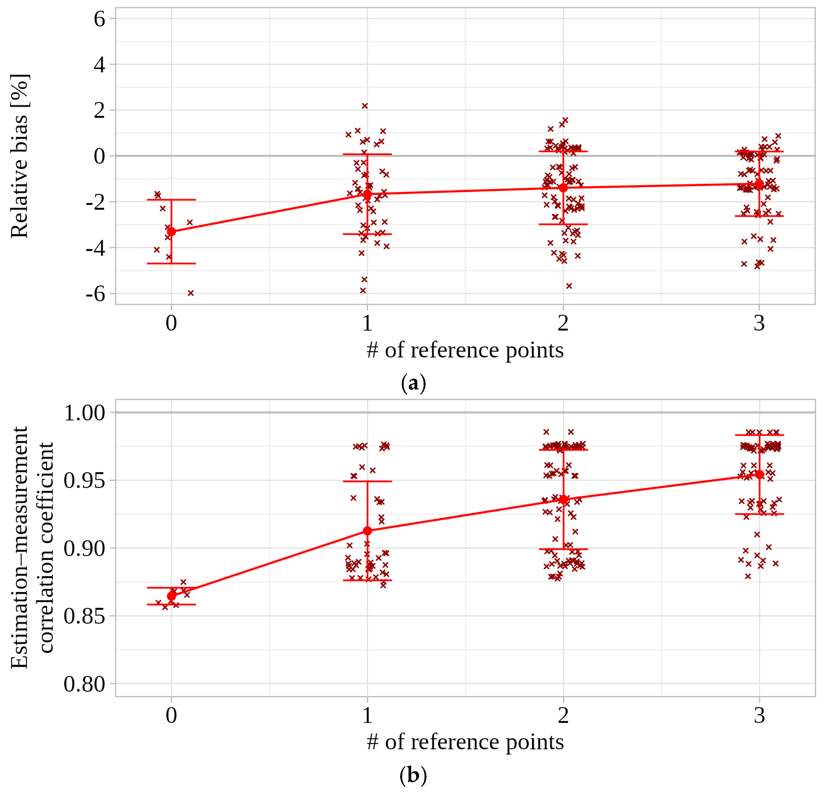
First, to examine the effect of increasing the number of reference points on estimation accuracy, we calculated the relative bias and the estimation–measurement correlation coefficient for each number of reference points (0–3). Here, 0 corresponds to CTRL, which uses no reference point, whereas 1–3 correspond to TC using one to three reference points. The results are shown in Figure 11. Individual samples are shown as scatter points, and red markers and lines indicate the mean values for each number of reference points with error bars representing ±1 standard deviation. For relative bias, the samples became less dispersed and tended to be distributed closer to 0% as the number of reference points increased. The estimation–measurement correlation coefficient also tended to take larger values as the number of reference points increased, indicating that estimation accuracy can improve as more reference points are used. This result indicates that, within the study area, estimation accuracy can be improved by increasing the number of reference points.

Figure 11. Effect of increasing the number of reference points on estimation accuracy: (a) relative bias and (b) estimation–measurement correlation coefficient.

However, these results also reflect the fact that, as the number of reference points increases, it becomes more likely that the set includes a reference point that is strongly related to the target point (i.e., has a high reference–target correlation coefficient). In other words, the apparent effect of increasing the number of reference points may be confounded with the increased probability of including the most suitable reference point. Therefore, to separate these effects as much as possible, we focus on the two-reference-point case and perform the following analysis.

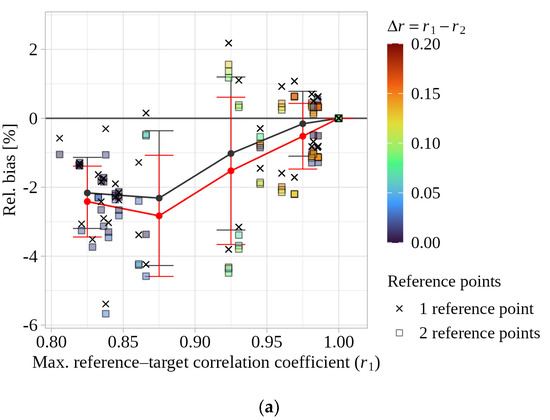
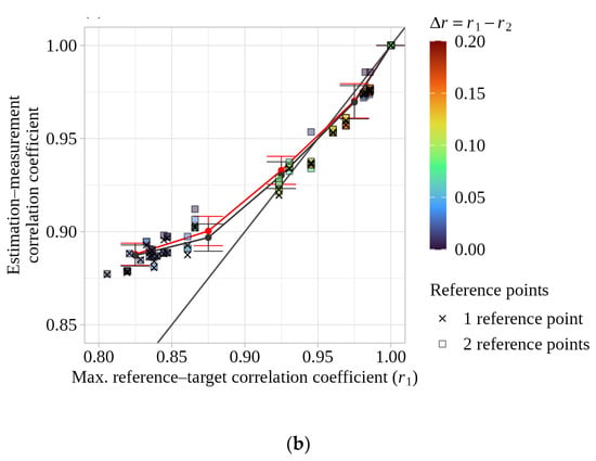
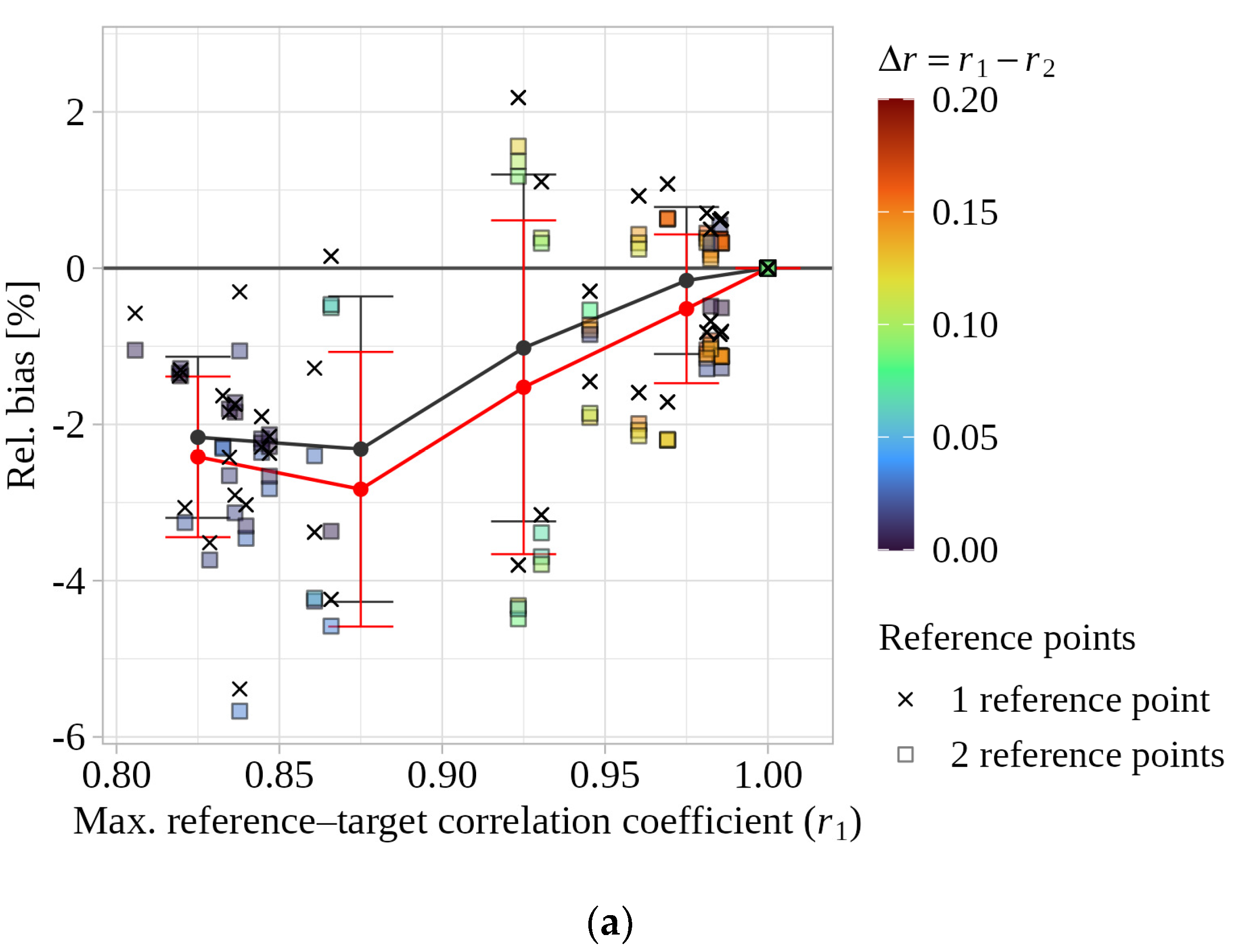
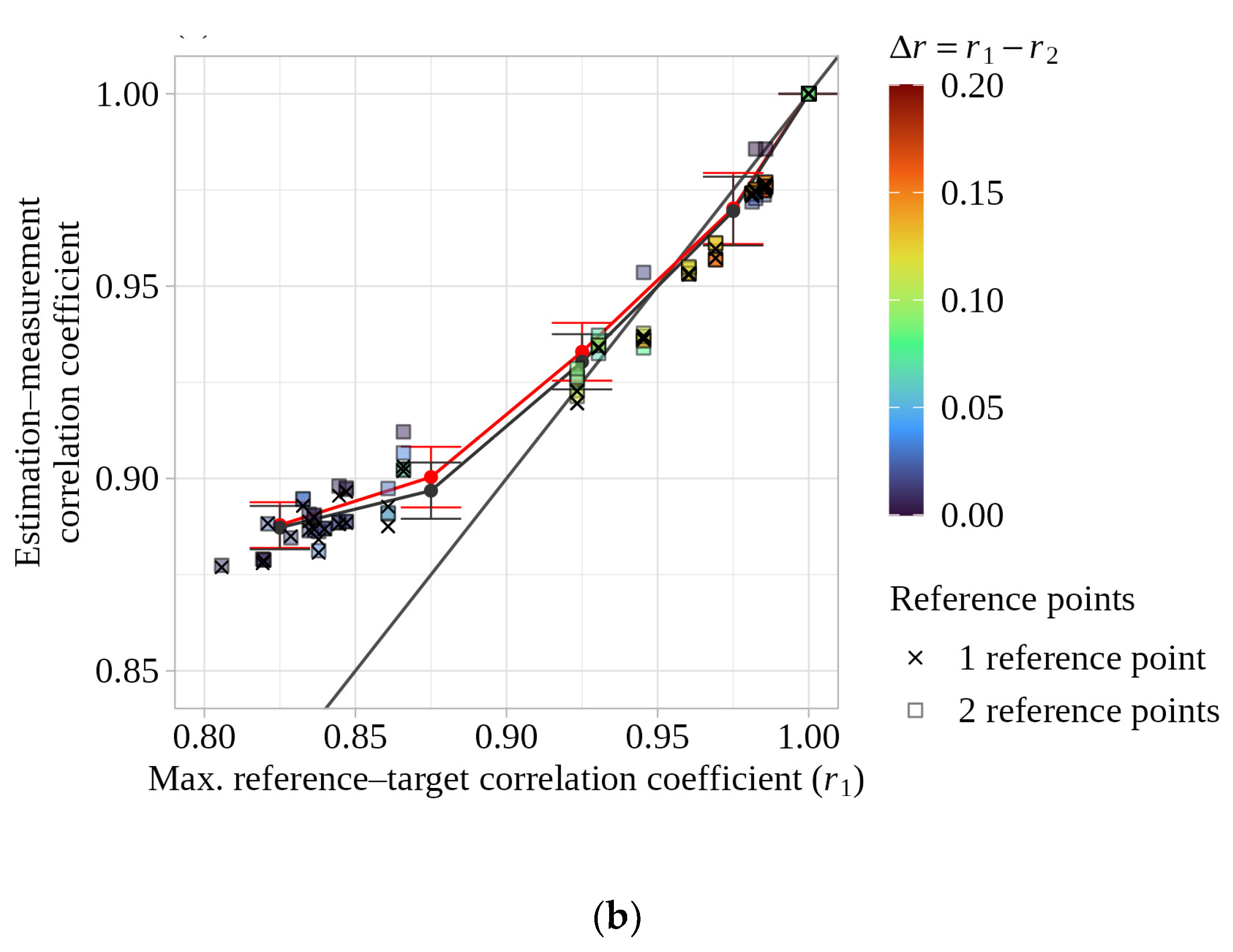
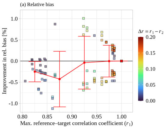
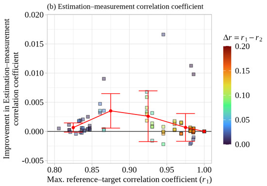
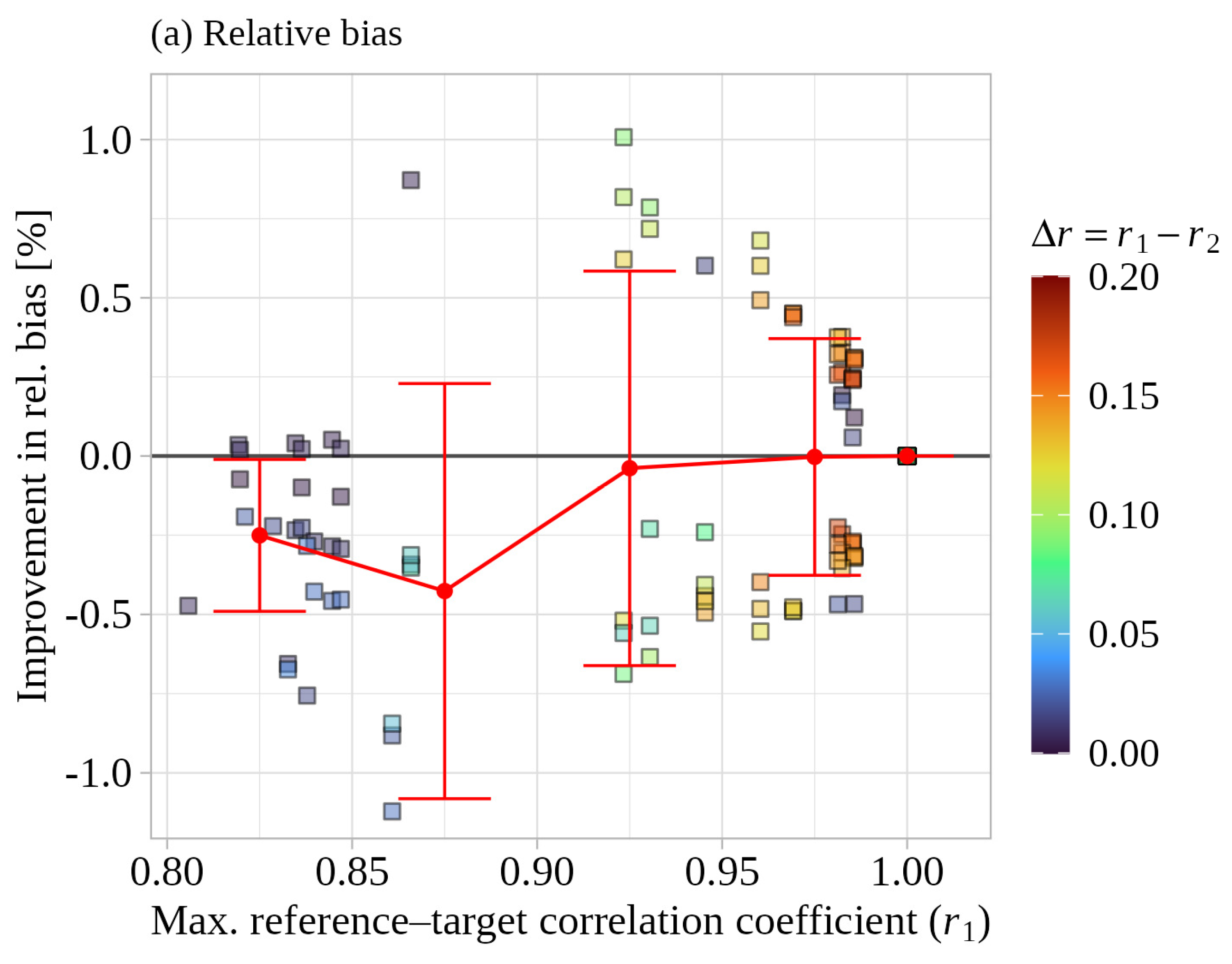
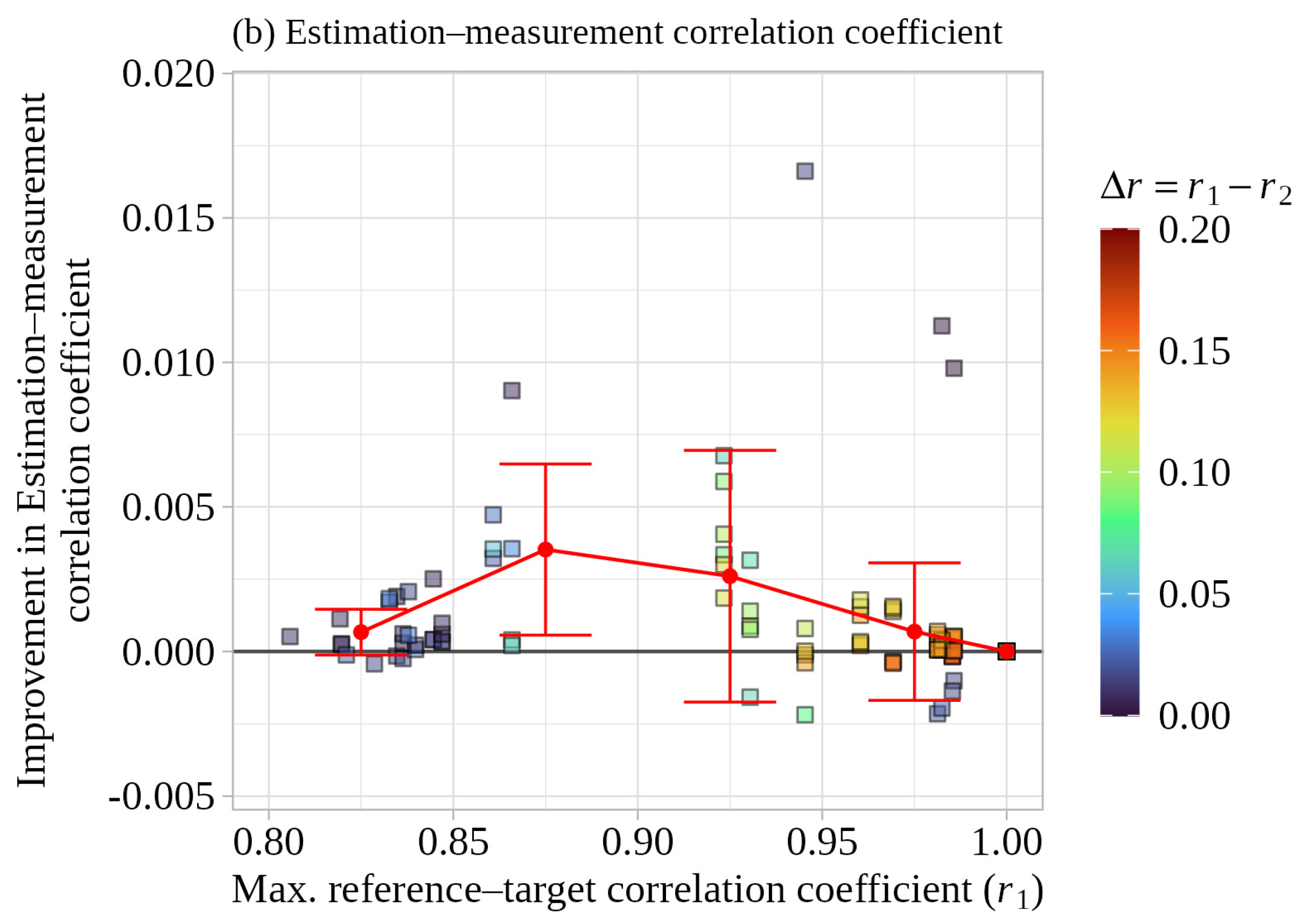
In Figure 12, for each two-reference-point sample, we define $r_1$ as the larger and $r_2$ as the smaller reference–target correlation coefficient of the two reference points with respect to the target point. Two panel plots show (a) the relative bias and (b) the estimation–measurement correlation coefficient, respectively, against $r_1$. Cross makers denote the corresponding single-reference samples, in which only the reference point associated with $r_1$ is used, whereas square markers denote the two-reference-point samples; the fill color of each square marker indicates the difference in the two correlation coefficients, $\mathsf{\Delta }r(=r_1-r_2)$. Thus, the difference between the cross and square makers represents the effect of adding the second reference point ($r_2$) to the best single reference point ($r_1$). Gray and red markers and lines denote the bin-averaged statistics for the single- and two-reference-point cases, respectively, and the error bars represent mean ± 1 standard deviation. In addition, to quantify the improvement of the two-reference-point case relative to the best single-reference case, Figure 13 shows the improvements in the absolute relative bias (defined as $\mid {\mathrm{b}\mathrm{i}\mathrm{a}\mathrm{s}}_{\mathrm{s}\mathrm{i}\mathrm{n}\mathrm{g}\mathrm{l}\mathrm{e}-\mathrm{r}\mathrm{e}\mathrm{f}}\mid -\mid {\mathrm{b}\mathrm{i}\mathrm{a}\mathrm{s}}_{\mathrm{t}\mathrm{w}\mathrm{o}-\mathrm{r}\mathrm{e}\mathrm{f}}\mid$) and in the estimation–measurement correlation coefficient (defined as ${\mathrm{C}.\mathrm{C}}_{\mathrm{t}\mathrm{w}\mathrm{o}-\mathrm{r}\mathrm{e}\mathrm{f}}-{\mathrm{C}.\mathrm{C}.}_{\mathrm{s}\mathrm{i}\mathrm{n}\mathrm{g}\mathrm{l}\mathrm{e}-\mathrm{r}\mathrm{e}\mathrm{f}}\mid$), respectively, where positive values indicate improvement. Red markers and lines denote the bin-averaged improvements, and the error bars represent mean ± 1 standard deviation. In Figure 13, as in Figure 12, the fill color of each square marker indicates the difference between the two reference–target correlation coefficients, $\mathsf{\Delta }r(=r_1-r_2)$.

Figure 12. Estimation accuracy of the single- and two-reference-point cases as a function of the maximum reference–target correlation at Ishikari: (a) relative bias and (b) estimation–measurement correlation coefficient. The fill color of each square marker indicates the difference between the two reference–target correlation coefficients, $\mathsf{\Delta }r=r_1-r_2$.

Figure 13. Accuracy improvement obtained by adding a second reference point as a function of the maximum reference–target correlation at Ishikari: (a) improvement in absolute relative bias and (b) improvement in estimation–measurement correlation coefficient. The fill color of each square marker indicates $\mathsf{\Delta }r=r_1-r_2$, as in Figure 12.

When the two-reference-point samples are compared with the corresponding single-reference samples, the relative bias changes little on average when $r_1$ is in the range of 0.90–1.00. In the range of $r_1=0.80$–0.90, some samples exhibit a slight deterioration; however, in both ranges, most samples remain within approximately ±0.5%, and both improvements and degradations are observed. For the estimation–measurement correlation coefficient, although improvements are relatively more frequent when $r_1$ is in the range of 0.85–0.95, the magnitude of the improvement is less than 0.005 in most samples. These results suggest that the accuracy gain obtained by using two reference points, by itself, is very limited.

5. Discussion

5.1. Case of a Single Reference Point

In our previous study, Maruo and Ohsawa [30], we investigated land–offshore extrapolation, in which winds at offshore target points are estimated using an onshore reference point located along the coastline. In contrast, the present study focuses on offshore–offshore extrapolation, where offshore reference points are used to estimate winds at offshore target points, reflecting the recent spread of scanning-lidar deployments. Although the characteristics of the reference points differ between the two studies, both confirm that wind estimation accuracy depends strongly on the reference–target correlation. Moreover, the previous study fixed the correction coefficient $\alpha$—which represents the degree to which the error vector obtained at the reference point is applied to the target point—to 1. In terms of estimation–measurement correlation coefficient, the previous study showed that TC provides effective correction relative to CTRL when the reference–target correlation coefficient is high (approximately $r_{MEAS,i}\gtrsim 0.90$), whereas it may not be effective when the correlation is low (approximately $r_{MEAS,i}\lesssim 0.85$). However, because the lowest reference–target correlation coefficient bin considered in that study was 0.85–0.90, samples with smaller correlations could not be validated. In the present study, by using a broader set of samples down to the 0.75–0.80 bin, we were able to demonstrate the tendency anticipated in the previous work. This tendency is likely to arise because, as the relationship between the reference and target points weakens, the TC error vector derived at the reference point becomes less representative of the “true” error vector at the target point. While it should be noted that the Ishikari samples do not include data around 0.90, this limitation does not materially affect this interpretation presented below.

In the previous study, to mitigate this tendency, it was proposed that the correction coefficient should be reduced according to the relationship between the reference and target points. Accordingly, in the present study, using data from two sites (Ishikari and Yuri-Honjo), we defined ${\alpha }_i$ as the correction coefficient that maximizes wind estimation accuracy, and investigated its relationship with the reference–target correlation coefficient. We showed that this relationship can be represented by a simple linear regression with a very high coefficient of determination ($0.96$). Moreover, in practical wind-resource assessments, the reference–target correlation coefficient cannot be obtained from measurement data at the target point, and therefore must be inferred from WRF-simulated results. We thus examined, for the same two sites, the relationship between the reference–target correlation coefficient derived from WRF-simulated results and that derived from the measurements, and found that it can also be expressed by a linear regression with a similarly high coefficient of determination ($0.96$).

Using these two relationships, we then evaluated the accuracy of TC-pred, in which the correction coefficient ${\alpha }_i$ is predicted from WRF-simulated results. The accuracy indicators of TC-pred were almost identical to those of TC-ideal, which directly searches for the optimal ${\alpha }_i$ for each reference–target pair (i.e., determines the optimal value with knowledge of the answer). This is likely attributable less to the high coefficient of determination of the empirical formula than to the shape of the estimation–measurement correlation coefficient function with respect to $\alpha$ shown in Figure 7, which suggests that the accuracy does not change substantially even if the estimation of ${\alpha }_i$ involves some error.

Based on the results of this study, the methodological framework of TC-pred is expected to be applicable to various types of nearshore areas. The two empirical regression relationships derived in this study were effective for estimating wind conditions at the two Japanese nearshore sites examined here. However, the direct applicability of these empirical relationships to other coastal regions and climatic regimes has not yet been fully validated. Therefore, further validation is required to confirm whether they hold at different sites, in years, and under meteorological conditions. For practical application to other regions, including both nearshore and offshore areas, we thus recommend that, when measurements are available at multiple locations, the regression coefficients of the two empirical relationships be re-derived wherever possible, or at least checked against local measurements if re-derivation is not feasible.

5.2. Case of Multiple Reference Points

In this study, we also examined an extension of the TC method to cases where multiple reference points are available, and evaluated its estimation accuracy. In the multiple-reference-point TC framework, the contribution from each reference point $i$ is expressed as ${\alpha }_i{w}_i$, i.e., the product of a correction coefficient ${\alpha }_i$ (based on the reference–target correlation coefficient) and a weighting coefficient $w_i$ (which distributes the contribution among multiple reference points). Here, ${\alpha }_i$ is taken as the value that maximizes the estimation–measurement correlation coefficient in the single-reference case, and $w_i$ is defined using ${\alpha }_i$ as an index of the relative relationship between each reference point and the target point—a quantity analogous to distance—and is constructed to satisfy consistency such that, when estimating at a reference point, the estimate matches the reference point itself.

Using the measurement data at Ishikari, we validated the estimation accuracy and found that, as the number of reference points increases, the dispersion of relative bias decreases and the estimation–measurement correlation coefficient tends to increase. However, because the reference–target combinations available for validation are limited to those listed in Table 5, increasing the number of reference points inevitably increases the probability of including a reference point that is strongly related to the target point (i.e., has a high reference–target correlation coefficient). Thus, the apparent benefit of using more reference points must be separated from any synergistic effect of using multiple reference points. Focusing therefore on the two-reference-point case, we define $r_1$ as the larger and $r_2$ as the smaller of the two reference–target correlation coefficients, and evaluate the incremental effect of adding the second reference point ($r_2$) relative to the best single-reference case (using only $r_1$). The results at Ishikari show that changes in bias are mixed (both improvements and degradations) with little overall tendency, and that the improvement in estimation–measurement correlation coefficient is very limited, being less than 0.005 in most samples. This behavior is consistent with the structure of the proposed method: since $0\le {\alpha }_i\le 1$ and $0\le w_i\le 1$, it follows that ${\alpha }_i{w}_i\le {\alpha }_i$. Therefore, when $r_2$ is low, ${\alpha }_2$ is small, and the contribution from the second reference point is further suppressed by the weighting coefficient $w_2$, making its net impact small when $r_1$ is already sufficiently high (see also Figure 10).

A more detailed assessment would require a sensitivity study using alternative weighting functions. However, as shown in Figure 7 for the single-reference case, the sensitivity of the estimation–measurement correlation coefficient to $\alpha$ is not large in the vicinity of the $\alpha$ value yielding the highest estimation–measurement correlation coefficient. This suggests that, even if a more advanced weighting function were devised, the resulting improvement in accuracy would likely be limited.

The Ishikari samples suggest that, in the context of conducting wind estimation using a TC-type approach, when multiple measurement points are designed, it would be more cost-effective—from the viewpoint of suppressing the uncertainty in wind estimation accuracy for the whole of the target sea area—to determine the measurement points so as to increase the coverage of correlations above a certain threshold by placing points with different representativeness such that a high $r_1$ can be secured for any target within the target sea area, rather than to “substantially improve the accuracy for the same target by adding points (i.e., by combining multiple measurement points).” This can be achieved by generating an inter-point correlation map—using each candidate measurement point as a reference point—from high-resolution mesoscale model simulations prior to finalizing the measurement design.

It should be noted that this interpretation is based on validation in a single area; therefore, further validation in other coastal and offshore areas is required to confirm its generalizability.

5.3. Relationship Between the Reference–Target Correlation and Distance

In this study, as in the previous study, Maruo and Ohsawa [30], the correlation coefficient between the reference point and the target point, based on measured 10 min mean wind speeds, was used as an indicator of the relationship between the two points. In general, distance is used as standard parameter for evaluating the effective range of a reference point (i.e., the representative radius). Therefore, this section examines the relationship between distance and the correlation coefficient.

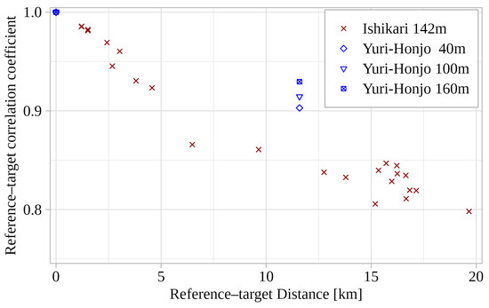
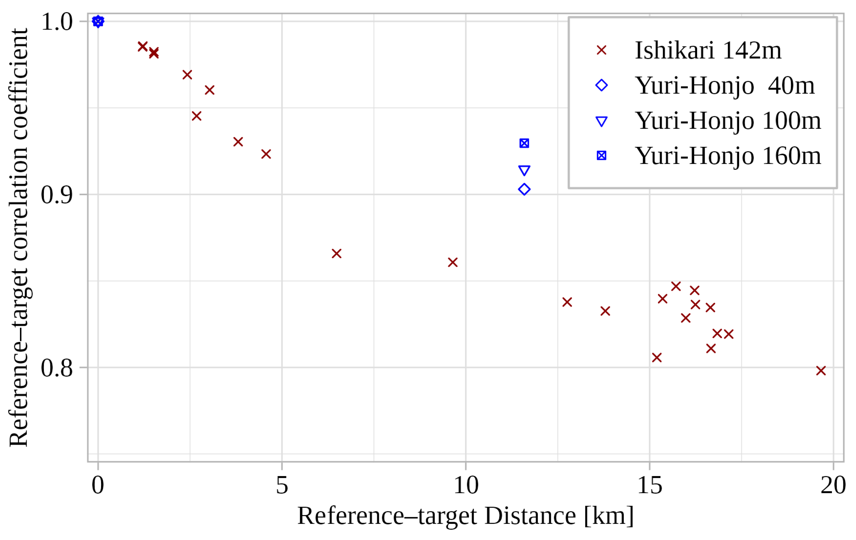
Figure 14 shows the relationship between the inter-point distance and the corresponding correlation coefficient at Ishikari and Yuri-Honjo. At both sites, the inter-point correlation exhibits a decreasing trend with increasing distance, consistent with the generally known tendency. This decreasing trend in correlation can be attributed to reduced measurement representativeness caused by atmospheric phenomena occurring at comparable or slightly larger spatial scales, such as internal boundary layers and land–sea breezes caused by land–sea contrasts in surface roughness and thermodynamic conditions, as well as flow modification caused by onshore terrain inhomogeneity.

Figure 14. Relationship between reference–target distance and correlation at the two nearshore sites (Ishikari and Yuri-Honjo). Red symbols denote Ishikari samples at 142 m, while blue symbols denote Yuri-Honjo samples at 40, 100 and 160 m for cross-site assessment.

Figure 14 shows the Yuri-Honjo samples exhibit a smaller decrease in correlation with increasing distance than the Ishikari samples. As shown in Section 3, the estimation accuracy of TC-pred is strongly related to the inter-point correlation. In light of this relationship, the observed difference in the decline trend of the correlation with distance between Ishikari and Yuri-Honjo suggests that the effective range of TC-pred also varies by site. Therefore, when estimating the effective range of reference points used in TC-pred, the inter-point correlation coefficient should be used instead of the inter-point distance.

Although the above discussion pertains to the effective range of TC-pred, it could also be applicable to the evaluation of inter-point relationships in general wind condition estimation.

5.4. Limitations of the Present Validation

Because annual wind speed estimation accuracy is of primary importance in wind resource assessment, this study developed the TC-pred framework and evaluated it over a one-year period without classification by atmospheric stability or wind direction sector. Although these factors may affect both the accuracy of WRF-simulated near-surface wind fields in nearshore areas and the empirical relationships used in TC-pred, their effects were not separately investigated in this study. Therefore, future work should clarify the dependence of the WRF error characteristics and the empirical relationships on these factors.

5.5. Applicable Scope of This Study

We note that site-specific wind condition evaluations generally involve turbulence measurements and the estimation of extreme wind speeds for wake assessment and turbine design; however, this study focuses solely on wind resource assessment, and these aspects are beyond the scope of the present work.

6. Conclusions

In this study, using scanning lidar measurements and high-resolution WRF simulations from two nearshore areas in Japan, we developed two extensions of the Temporal Correction (TC) method, which corrects wind fields generated by WRF using on-site measurements.

• When using a single measurement point for correction, we derived two empirical formulas to predict appropriate correction coefficients based on reference–target correlation coefficients of wind speed obtained from WRF simulations and developed a method (TC-pred) using these formulas. TC-pred was shown to have higher wind speed estimation accuracy and a broader range of applicability than the conventional TC method.
• Furthermore, we extended the TC-pred method to allow the use of multiple measurement points as references by introducing a weighting formula for each reference point. Wind speed estimation accuracy improved as the number of reference points increased, primarily because the probability of including reference points with high reference–target correlation coefficients increased. This suggests that it is effective for the suppression of wind estimation uncertainty to determine measurement layout such that the correlation coefficient between at least one reference point and each target point in the target area exceeds a certain value.

These results suggest that the TC-pred framework has potential applicability beyond the two Japanese nearshore sites examined here, while the empirical regression coefficients require site-specific verification before practical use.

In future work, we plan to modify the TC-pred method so that the correction coefficient α depends on the correlation coefficient specific to atmospheric stability class and wind direction sector.

References

- MEASNET. Evaluation of Site-Specific Wind Conditions, Version 3; MEASNET: Madrid, Spain, 2022; p. 64.
- Troen, I.; Petersen, E.L. European Wind Atlas; Risø National Laboratory: Roskilde, Denmark, 1989. [Google Scholar]
- Dayal, K.K.; Cater, J.E.; Kingan, M.J.; Bellon, G.D.; Sharma, R.N. Wind resource assessment and energy potential of selected locations in Fiji. Renew. Energy 2021, 172, 219–237. [Google Scholar] [CrossRef] [Scilit]
- Ishihara, T.; Hibi, K. Numerical study of turbulent wake flow behind a three-dimensional steep hill. Wind Struct. 2002, 5, 317–328. [Google Scholar] [CrossRef] [Scilit] [PubMed]
- Deen, S.A.; Yamaguchi, A.; Ishihara, T. A physical approach to wind speed prediction for wind energy forecasting. In Proceedings of the Fourth International Symposium on Computational Wind Engineering, Yokohama, Japan, 16–19 July 2006; pp. 349–352. [Google Scholar]
- Uchida, T.; Ohya, Y. Micro-siting technique for wind turbine generators by using large-eddy simulation. J. Wind Eng. Ind. Aerodyn. 2008, 96, 2121–2138. [Google Scholar] [CrossRef] [Scilit]
- Uchida, T. Computational fluid dynamics approach to predict the actual wind speed over complex terrain. Energies 2018, 11, 1694. [Google Scholar] [CrossRef] [Scilit]
- Watanabe, C.; Hirata, K. Offshore Wind in Japan Policy Agenda and Prospects; Climate Integrate: Tokyo, Japan, 2024; p. 29. [Google Scholar]
- Stull, R.B. An Introduction to Boundary Layer Meteorology, 1st ed.; Springer: Dordrecht, The Netherlands, 1988. [Google Scholar]
- De Tomasi, F.D.; Miglietta, M.M.; Perrone, M.R. The growth of the planetary boundary layer at a coastal site: A case study. Bound.-Layer Meteorol. 2011, 139, 521–541. [Google Scholar] [CrossRef] [Scilit]
- Floors, R.; Batchvarova, E.; Gryning, S.-E.; Hahmann, A.N.; Peña, A.; Mikkelsen, T. Atmospheric boundary layer wind profile at a flat coastal site—Wind speed lidar measurements and mesoscale modeling results. Adv. Sci. Res. 2011, 6, 155–159. [Google Scholar] [CrossRef] [Scilit]
- Dörenkämper, M.; Optis, M.; Monahan, A.; Steinfeld, G. On the offshore advection of boundary-layer structures and the influence on offshore wind conditions. Bound.-Layer Meteorol. 2015, 155, 459–482. [Google Scholar] [CrossRef] [Scilit]
- Lo Feudo, T.L.; Calidonna, C.R.; Avolio, E.; Sempreviva, A.M. Study of the vertical structure of the coastal boundary layer integrating surface measurements and ground-based remote sensing. Sensors 2020, 20, 6516. [Google Scholar] [CrossRef] [Scilit]
- Bauer, H.-S.; Muppa, S.K.; Wulfmeyer, V.; Behrendt, A.; Warrach-Sagi, K.; Späth, F. Multi-nested WRF Simulations for studying planetary boundary layer processes on the turbulence-permitting scale in a realistic mesoscale environment. Tellus A 2020, 72, 1761740. [Google Scholar] [CrossRef] [Scilit]
- Kikuchi, Y.; Fukushima, M.; Ishihara, T. Assessment of a coastal offshore wind climate by means of mesoscale model simulations considering high-resolution land use and sea surface temperature data sets. Atmosphere 2020, 11, 379. [Google Scholar] [CrossRef] [Scilit]
- Konagaya, M.; Ohsawa, T.; Mito, T.; Misaki, T.; Maruo, T.; Baba, Y. Estimation of nearshore wind conditions using onshore observation data with computational fluid dynamic and mesoscale models. Resources 2022, 11, 100. [Google Scholar] [CrossRef] [Scilit]
- Konagaya, M.; Ohsawa, T.; Itoshima, Y.; Kambayashi, M.; Leonard, E.; Tromeur, E.; Misaki, T.; Shintaku, E.; Araki, R.; Hamada, K. Estimation of wind conditions in the offshore direction using multiple numerical models and in situ observations. Energies 2025, 18, 3000. [Google Scholar] [CrossRef] [Scilit]
- Skamarock, W.C.; Klemp, J.B.; Dudhia, J.; Gill, D.O.; Liu, Z.; Berner, J.; Wang, W.; Powers, J.G.; Duda, M.G.; Barker, D.M.; et al. A Description of the Advanced Research WRF Model Version 4; NCAR: Boulder, CO, USA, 2019. [Google Scholar]
- Sempreviva, A.M.; Barthelmie, R.J.; Pryor, S.C. Review of methodologies for offshore wind resource assessment in European seas. Surv. Geophys. 2008, 29, 471–497. [Google Scholar] [CrossRef] [Scilit]
- Hahmann, A.N.; Sīle, T.; Witha, B.; Davis, N.N.; Dörenkämper, M.; Ezber, Y.; García-Bustamante, E.; González-Rouco, J.F.; Navarro, J.; Olsen, B.T.; et al. The making of the new European wind atlas—Part 1: Model sensitivity. Geosci. Model Dev. 2020, 13, 5053–5078. [Google Scholar] [CrossRef] [Scilit]
- Dörenkämper, M.; Olsen, B.T.; Witha, B.; Hahmann, A.N.; Davis, N.N.; Barcons, J.; Ezber, Y.; García-Bustamante, E.; González-Rouco, J.F.; Navarro, J.; et al. The making of the new European wind atlas—Part 2: Production and evaluation. Geosci. Model Dev. 2020, 13, 5079–5102. [Google Scholar] [CrossRef] [Scilit]
- Papanastasiou, D.K.; Melas, D.; Lissaridis, I. Study of wind field under sea breeze conditions; An application of WRF model. Atmos. Res. 2010, 98, 102–117. [Google Scholar] [CrossRef] [Scilit]
- Storm, B.; Dudhia, J.; Basu, S.; Swift, A.; Giammanco, I. Evaluation of the weather research and forecasting model on forecasting low-level jets: Implications for wind energy. Wind Energy 2009, 12, 81–90. [Google Scholar] [CrossRef] [Scilit]
- Reen, B. A Brief Guide to Observation Nudging in WRF; Battlefield Environment Division, Army Research Laboratory: Adelphi, MD, USA, 2016. [Google Scholar]
- Stauffer, D.R.; Seaman, N.L. Use of four-dimensional data assimilation in a limited-area mesoscale model. Part I: Experiments with synoptic-scale data. Mon. Weather Rev. 1990, 118, 1250–1277. [Google Scholar] [CrossRef] [Scilit]
- Gryning, S.-E.; Batchvarova, E.; Floors, R. A study on the effect of nudging on long-term boundary layer profiles of wind and Weibull distribution parameters in a rural coastal area. J. Appl. Meteorol. Climatol. 2013, 52, 1201–1207. [Google Scholar] [CrossRef] [Scilit]
- Mylonas, M.P.; Barbouchi, S.; Herrmann, H.; Nastos, P.T. Sensitivity analysis of observational nudging methodology to reduce error in wind resource assessment (WRA) in the North Sea. Renew. Energy 2018, 120, 446–456. [Google Scholar] [CrossRef] [Scilit]
- Misu, Y.; Ishihara, T. Prediction of frequency distribution of strong crosswind in a control section for train operations by using onsite measurement and numerical simulation. J. Wind Eng. Ind. Aerodyn. 2018, 174, 69–79. [Google Scholar] [CrossRef] [Scilit]
- Qian, G.-W.; Ishihara, T. A novel probabilistic power curve model to predict the power production and its uncertainty for a wind farm over complex terrain. Energy 2022, 261, 125171. [Google Scholar] [CrossRef] [Scilit]
- Maruo, T.; Ohsawa, T. Wind estimation methods for nearshore wind resource assessment using high-resolution WRF and coastal onshore measurements. Wind 2025, 5, 17. [Google Scholar] [CrossRef] [Scilit]
- Peña, A.; Mann, J. Turbulence measurements with dual-Doppler scanning lidars. Remote Sens. 2019, 11, 2444. [Google Scholar] [CrossRef] [Scilit]
- Simon, E.; Courtney, M. A Comparison of Sector-Scan and Dual Doppler Wind Measurements at Høvsøre Test Station—One Lidar or Two? Technical Report DTU Wind Energy E-0112(EN); DTU Wind Energy: Roskilde, Denmark, 2016. [Google Scholar]
- Misaki, T. A Study on Improving the Accuracy of Coastal Wind Speeds Simulated by Mesoscale Model. Ph.D. Thesis, Kobe University, Kobe, Japan, 2020; p. 78. [Google Scholar]
- Kvålseth, T.O. Cautionary note about R2. Am. Stat. 1985, 39, 279–285. [Google Scholar] [CrossRef] [Scilit]
Disclaimer/Publisher’s Note: The statements, opinions and data contained in all publications are solely those of the individual author(s) and contributor(s) and not of MDPI and/or the editor(s). MDPI and/or the editor(s) disclaim responsibility for any injury to people or property resulting from any ideas, methods, instructions or products referred to in the content. |
© 2026 by the authors. Licensee MDPI, Basel, Switzerland. This article is an open access article distributed under the terms and conditions of the Creative Commons Attribution (CC BY) license.