A Modeling Approach to Aggregated Noise Effects of Offshore Wind Farms in the Canary and North Seas ^†

Abstract

Offshore wind farms (OWFs) represent an increasingly important renewable energy source, yet their environmental impacts, particularly underwater noise, require systematic study. Estimating the operational source level (SL) of a single turbine and predicting sound pressure levels (SPLs) at sensitive locations can be challenging. Here, we integrate a turbine SL prediction algorithm with open-source propagation models in a Jupyter Notebook (version 7.4.7) to streamline aggregated SPL estimation for OWFs. Species-specific audiograms and weighting functions are included to assess potential biological impacts. The tool is applied to four planned OWFs, two in the Canary region and two in the Belgian and German North Seas, under conservative assumptions. Results indicate that at 10 m/s wind speed, a single turbine’s SL reaches 143 dB re 1 µPa in the one-third octave band centered at 160 Hz. Sensitivity analyses indicate that variations in wind speed can cause the operational source level at 160 Hz to increase by up to approximately 2 dB re 1 µPa²/Hz from the nominal value used in this study, while differences in sediment type can lead to transmission loss variations ranging from 0 to on the order of 100 dB, depending on bathymetry and range. Maximum SPLs of 112 dB re 1 µPa are predicted within OWFs, decreasing to ~50 dB re 1 µPa at ~100 km. Within OWFs, Low-Frequency (LF) cetaceans and Phocid Carnivores in Water (PCW) would likely perceive the noise; National Marine Fisheries Service (NMFS) marine mammals’ auditory-injury thresholds are not exceeded, but behavioral-harassment thresholds may be crossed. Outside the farms, only LF audiograms are crossed. In high-traffic North Sea regions, OWF noise is largely masked, whereas in lower-noise areas, such as the Canary Islands, it can exceed ambient levels, highlighting the importance of site-specific assessments, accurate ambient noise monitoring and propagation modeling for ecological impact evaluation.

1. Introduction

In the context of global warming, the green energy transition has become essential to reduce CO₂ emissions. As a result, offshore wind farms (OWFs) have gained significant attention from energy companies. With the increasing number of OWF implementation projects, it is crucial to assess their potential impacts on local marine ecosystems. One of the main concerns associated with OWFs is underwater noise emissions, which may pose serious threats to marine life [1]. Numerous studies have investigated the effects of anthropogenic noise on various marine species, and the scientific community continues to work on identifying the thresholds that trigger harmful effects or behavioral changes in different organisms [1,2]. In parallel, researchers are analyzing the specific source levels (SLs) emitted by different wind turbines. Noise spectrum prediction algorithms based on principal component analysis (PCA) combined with Gaussian process regression bridge knowledge gaps by enabling the prediction of SL spectra across different wind speeds [3]. Furthermore, noise propagation models, such as Range-dependent Acoustic Model (RAM) [4] and Bellhop [5], can estimate how sound disperses throughout the surrounding marine environment. However, integrating these models with SL prediction tools and ecological data remains complex, making it challenging to assess the underwater acoustic impact of specific OWF projects realistically and comprehensively.

To address this gap, we developed an integrated tool that combines SL spectrum prediction [3] with publicly available propagation models (RAM and Bellhop), all within a Jupyter Notebook framework. This tool allows for the estimation of the sound pressure level (SPL) spectrum at receiver locations, generated by multiple turbines from an OWF. In addition, the notebook incorporates known audiograms and weighting functions for various marine species [2] to evaluate potential biological impacts by comparing them to the predicted SPLs.

In this study, we apply the previously described prediction and propagation tool to four planned offshore wind farm (OWF) regions: Granadilla, Tenerife [6]; Tarahal, Gran Canaria [7]; the Princess Elisabeth I zone, Belgium [8]; and the N10.2 area, Germany [9]. We estimate the 1/3-octave band sound pressure levels (SPLs) at ecologically sensitive locations identified by the Natura 2000 network [10] and compare them with published audiograms [2], and with National Marine Fisheries Service (NMFS) recommended marine mammals harassment thresholds [11]. Additionally, we compare these levels with ambient noise measurements from the North Sea [12]. Due to a lack of publicly available records of ambient noise in the Canary region, we rely on canonical ambient curves for this area [13]. This approach enables an assessment of whether OWF-generated noise constitutes a significant additional acoustic input relative to existing ambient ocean noise levels.

2. Materials and Methods

2.1. Operational Wind Speed

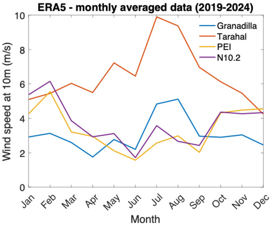
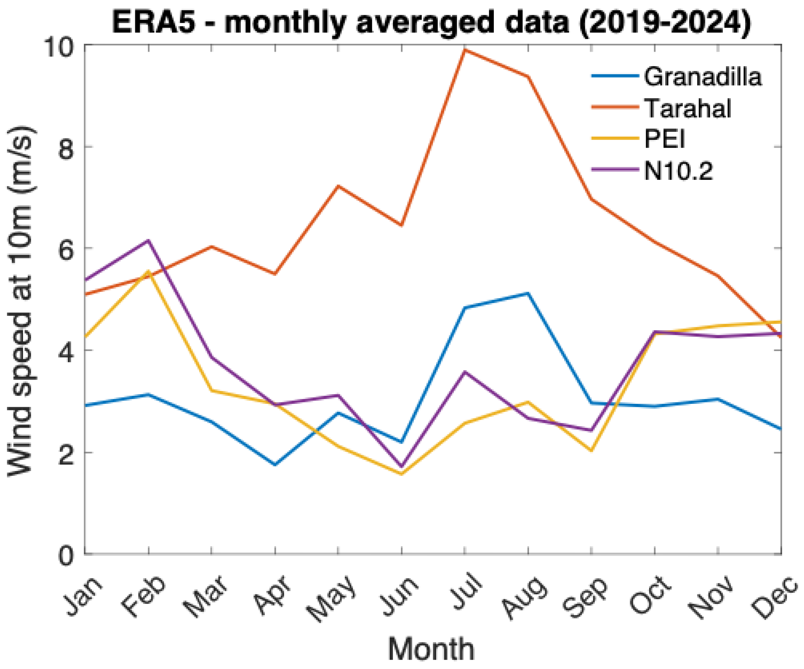
To adopt the most conservative case scenario, we use the maximum climatological wind speed at 10 m height from ERA5 reanalysis dataset [14] across all the OWF locations, which reaches 10 m/s. Figure 1 shows the monthly mean wind speed climatology for 2019–2024 for each OWF placement.

Figure 1. Monthly climatology of 10 m wind speed for each OWF, derived from the ERA5 reanalysis dataset.

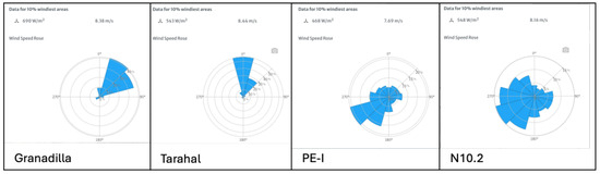
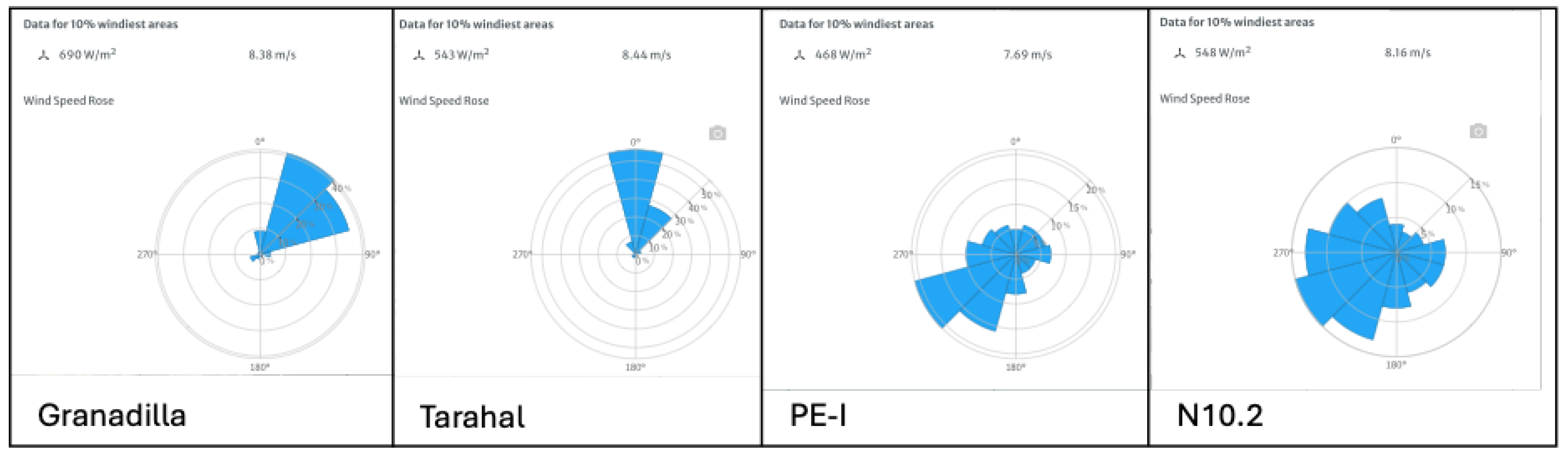
We contrast this 10 m/s threshold with the Global Wind Atlas [15], confirming that it is a conservative value on each of the OWF sites (Figure 2).

Figure 2. 10 m wind speed statistics from the Global Wind Atlas [15], evaluated at the center of each OWF.

2.2. Source Locations

We define turbine locations, based on defined potential placements found in publicly available sources, for Canary (Spain), Belgium, and German waters.

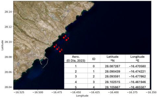
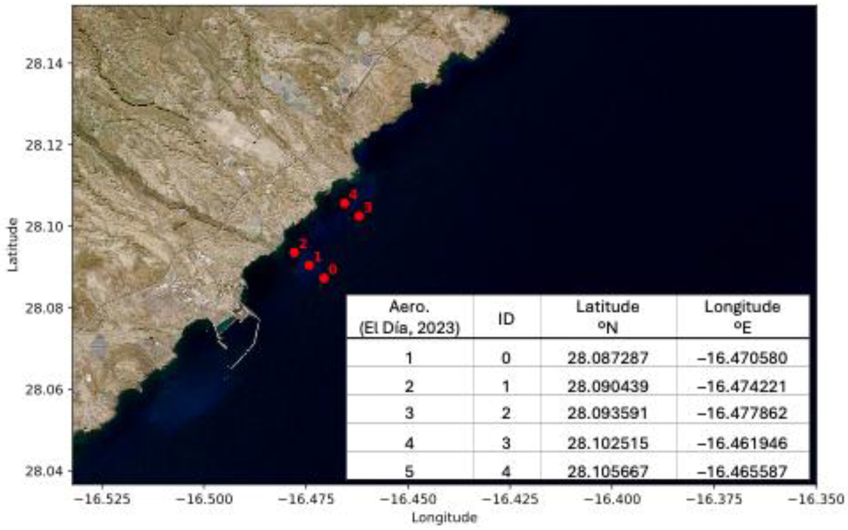
Figure 3 shows the Granadilla OWF turbines’ localization, from the draft layout of the Granadilla project [6]. The site is located approximately 2 km north-east of Granadilla port (Tenerife, Spain). The planned turbines at this location are expected to be fixed monopile structures.

Figure 3. Location map of the projected turbines for the Granadilla OWF. The table at the bottom right shows the geographical coordinates of the turbines, with the first column indicating the labels from the project draft and the second column the labels adopted in this study.

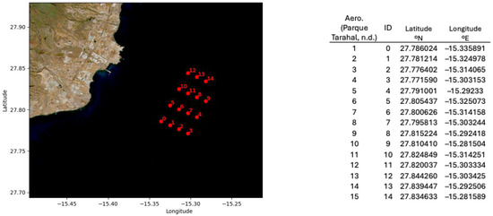
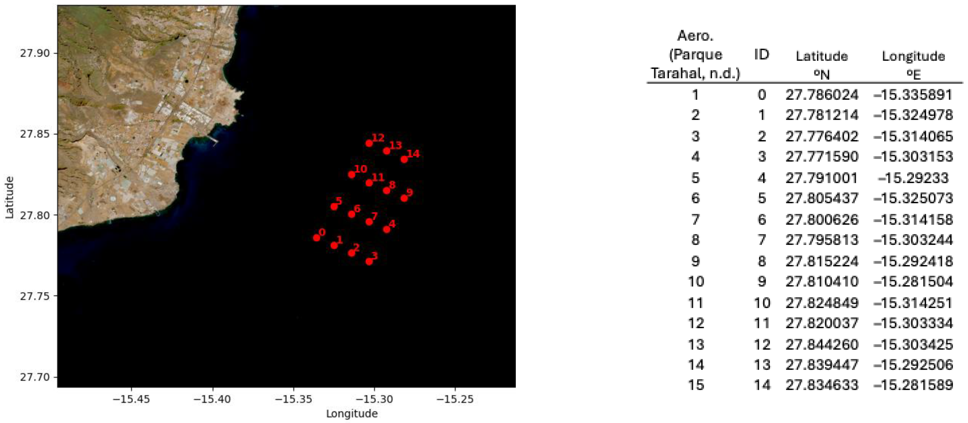
Figure 4 shows the locations of the Tarahal OWF turbines [7]. This OWF is planned to be approximately 10 km southeast of the Arinaga coast (Gran Canaria, Spain) and will feature floating turbines.

Figure 4. Location map of the projected turbines for the Tarahal OWF. The table at right shows the geographical coordinates of the turbines, with the first column indicating the labels from the project draft and the second column the labels adopted in this study.

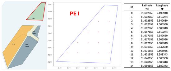
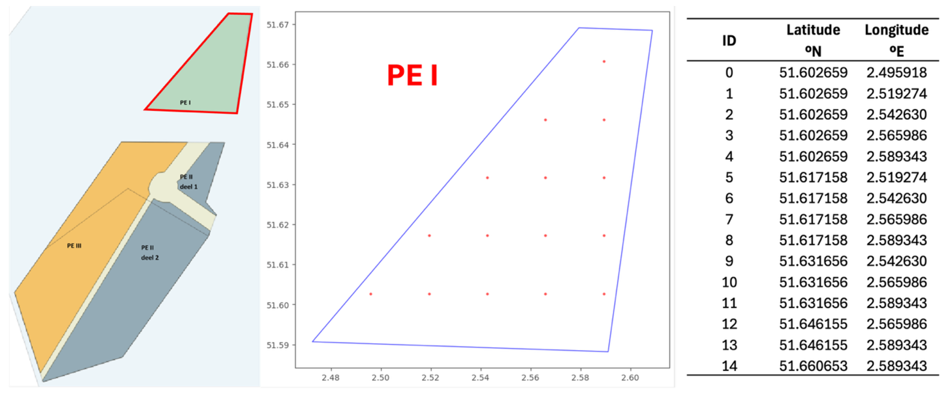
We selected the Princess Elisabeth Zone I (PEI) for the noise propagation analysis as it represents the furthest stage of development within Belgium’s offshore wind expansion plans [16]. Although the tender has been postponed until 2026, it remains the most advanced site under preparation, with a defined project area of 46 km² and a planned capacity of 700 MW. Since no preliminary draft of turbine positions is yet available, we assumed a layout with turbine locations separated by one mile in both longitude and latitude within the Princess Elisabeth Zone I (see Figure 5).

Figure 5. (Left) Location map of the Princess Elisabeth zones (Federal Public Service Economy, n.d. [8]). (Center) Assumed turbine locations within Princess Elisabeth Zone I (PEI). (Right) Table with the geographical coordinates of the turbines.

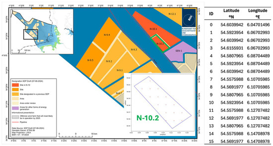
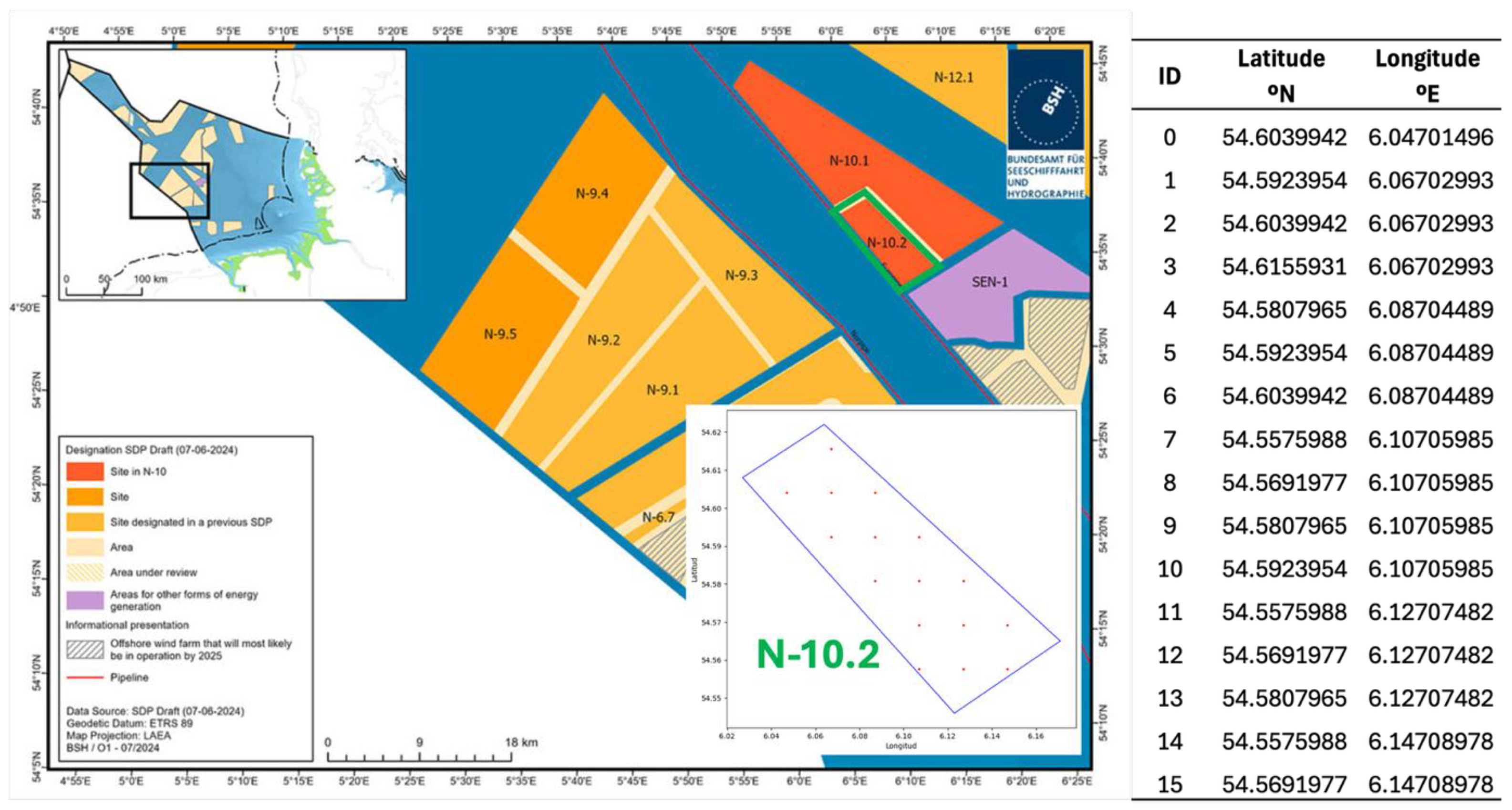
We have selected the German offshore wind development area N-10.2, shown in Figure 6, for the noise propagation analysis as it is among the most recently designated sites deemed suitable for construction and operation by the Federal Maritime and Hydrographic Agency (BSH) [9]. The area covers 31 km², is planned for an installed capacity of 500 MW, and is included in the upcoming 2025 tender, making it a clearly defined and advanced candidate for development. Since no preliminary draft of turbine positions is yet available, we assumed a layout with turbine locations separated by 0.5 miles in both longitude and latitude within the N-10.2 site.

Figure 6. (Left) Location map of the N-10.2 area for offshore energy within the North Sea Exclusive Economic Zone (EEZ), from Federal Maritime and Hydrographic Agency (BSH). (Center, inset) Zoomed-in layout showing the assumed turbine locations within N-10.2. (Right) Table with the geographical coordinates of the turbines.

2.3. Receiver Locations

Receiver locations representing vulnerable marine zones are selected using spatial data from NATURA 2000 [2110], focusing on areas protected under the Habitats Directive. Additionally, other sensitive areas from IDE Canarias (GRAFCAN) were chosen, cataloged as Reservas de la Biosfera (BIO) [17]. Finally, a receiver positioned at the center of the OWF turbines is estimated and denoted as INX (e.g., ING = INside Granadilla).

Table 1 represents the receiver locations adopted to study the potential impact of each OWF on these sites.

Table 1. Receiver locations adopted in this study for OWF noise propagation analysis.

OWF	ID	Description	Latitude °N	Longitude °E
Granadilla	ING	Inside OWF	28.095000	−16.465587
	TFE1	Natura 2000 Sebadales del sur de Tenerife (ES7020116) *	28.035364	−16.473202
	TFE2	BIO *	28.446869	−16.104856
	GC1	Natura 2000 Franja marina de Mogán (ES7010017)	27.902083	−15.889972
Tarahal	INT	Inside OWF	27.807925	−15.303244
	GC2	Natura 2000 Franja marina de Mogán (ES7010017)	27.705500	−15.597093
	GC3	Natura 2000 Sebadales de Playa del Inglés (ES7010056)	27.750467	−15.541356
	GC4	Natura 2000 Playa del Cabrón (ES7010053)	27.835319	−15.370708
	FTV1	Natura 2000 Espacio marino del oriente y sur de Lanzarote-Fuerteventura (ESZZ15002)	28.043689	−14.526958
	FTV2		28.041669	−14.316244
PEI	INP	Inside OWF	51.6219905	2.55820093
	BE	Natura 2000 Vlaamse Banken (BEMNZ0001)	51.226348	2.665838
	FR	Natura 2000 Récifs Gris-Nez Blanc-Nez (FR3102003)	50.953812	1.499381
	NL	Natura 2000 Voordelta (NL4000017)	51.576599	3.398938
N10.2	INN	Inside OWF	54.582971	6.100805
	DE1	Natura 2000 Borkum-Riffgrund (DE2104301)	53.855072	6.368749
	DE2	Natura 2000 Sylter Außenriff (DE1209301)	54.797312	7.303316
	NL2	Natura 2000 Doggersbank (NL2008001)	55.223200	3.767259
	NL3	Natura 2000 Klaverbank (NL2008002)	54.014082	3.088145

* indicates that the receiver location was adjusted to the nearest open-water area without interference when land obstructed the path between the source and receiver.

2.4. Bathymetry

Bathymetric information is retrieved from EMODnet [18]. We have integrated a tool to automatically download the required bathymetric subset based on the defined source and receiver coordinates. This tool interacts with the EMODnet ERDDAP server to select and temporarily download the relevant longitude, latitude, and depth data in .csv format.

For example, in a case where the area of interest spans latitudes from 27° to 28° N and longitudes from −15° to −14° E, the tool generates the following URL, which directly downloads the corresponding .csv file: https://erddap.emodnet.eu/erddap/griddap/dtm_2020_v2_e0bf_e7e4_5b8f.csv?elevation%5B(27):1:(28)%5D%5B(-15):1:(-14)].

By visiting this URL, the dataset is automatically downloaded in the .csv format, allowing its integration into the acoustic model workflow.

2.5. Sound Speed Profile

The sound speed profile (SSP) is estimated as [19]:

$$c=1449.2+4.6T-0.055T^2+0.00029T^3+\left(1.34-0.01T\right)\left(S-35\right)+0.016z$$

(1)

where c is the P-wave celerity (i.e., the underwater sound speed) (m/s), T is the temperature (°C), S is the salinity, and z is the depth (m). We downloaded temperature and salinity data from Copernicus Marine Service, relative to 1 July 2020 [20].

2.6. Seabed Geoacoustic Modeling

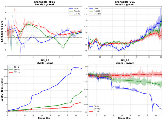
We performed a sensitivity analysis to evaluate the effect of different sediment types, representative of each OWF area, on the propagation of operational noise. By computing the differences between the propagated SPL obtained using one or another sediment type, at the prevailing frequencies of the OWF source levels, and averaging these differences along the water column, we assessed how sensitive the received SPL is to sediment selection. This analysis was carried out empirically, since irregular bathymetry strongly influences how sediments affect SPL. Three study cases were selected, each considering a single source. Two sections were analyzed in Tenerife (one nearshore and another extending toward Gran Canaria) and one in Belgian North Sea waters. Sections of SPL computed using each sediment type at the corresponding peak frequencies are provided in the Supplementary Materials, section A. Figure 7 presents the SPL differences along each section for the sediment types considered.

Figure 7. Depth-averaged difference of aggregated SPL modeling different sediment-type seabeds at various OWF-to-receiver sections (Granadilla-to-TFE1, Granadilla-to-GC1, and Princess Elisabeth I-to-BE). For visualization, the depth-averaged SPL difference curves were smoothed using a Gaussian filter with σ = 200 m, while transparent lines show the original, unfiltered data.

Selecting basalt for the Canary region and chalk for the North Sea represents a conservative assumption. Although chalk is not typically present in the upper sediment layers of the North Sea areas surrounding the OWFs considered in this study, modeling the seafloor as sand could lead to underestimates of SPL, since more consolidated layers above the sand often reflect sound more effectively. The comparison between chalk and basalt in the PEI_BE case is included to illustrate how part of the difference in modeled SPL between the Canary region and the North Sea is related to the sediment type used in the propagation modeling. This difference is largest at low frequencies, particularly at 50 Hz, where the SPL over basalt exceeds that over chalk by an average of 40 dB re 1 µPa at a range of 40 km.

2.7. Working Scheme and Assumptions

A detailed description of the workflow and the assumptions adopted in this study is provided in the Supplementary Materials, sections B and C.

3. Results

3.1. Theoretical Effect of an Additional Noise Source

Before starting with the OWF noise analysis, we first examine the combined effect of several identical sources, each with the same SPL (SPL₀). Specifically, we are interested in the incremental contribution ΔSPL(N) of the N-th additional source compared to the aggregated SPL from N−1 sources.

Starting from cumulative SPL definition (See Supplementary Materials, section B), and assuming SPL_i = SPL₀, we obtain:

$${SPL}_t\left(N\right)=10\log \sum _{i=1}^N {10}^{{\displaystyle \frac{{SPL}_0}{10}}}=10 \log \left(N {10}^{{\displaystyle \frac{{SPL}_0}{10}}}\right) =10\log N+{SPL}_0$$

(2)

Therefore, the incremental contribution of the N-th source is:

$$\Delta SPL\left(N\right)=SPL\left(N\right)-SPL\left(N-1\right)=10 log \left({\displaystyle \frac{N}{N-1}}\right)$$

(3)

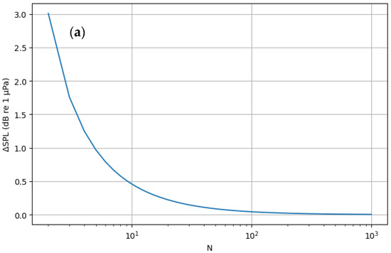
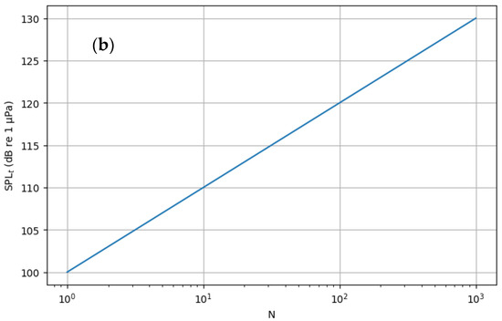
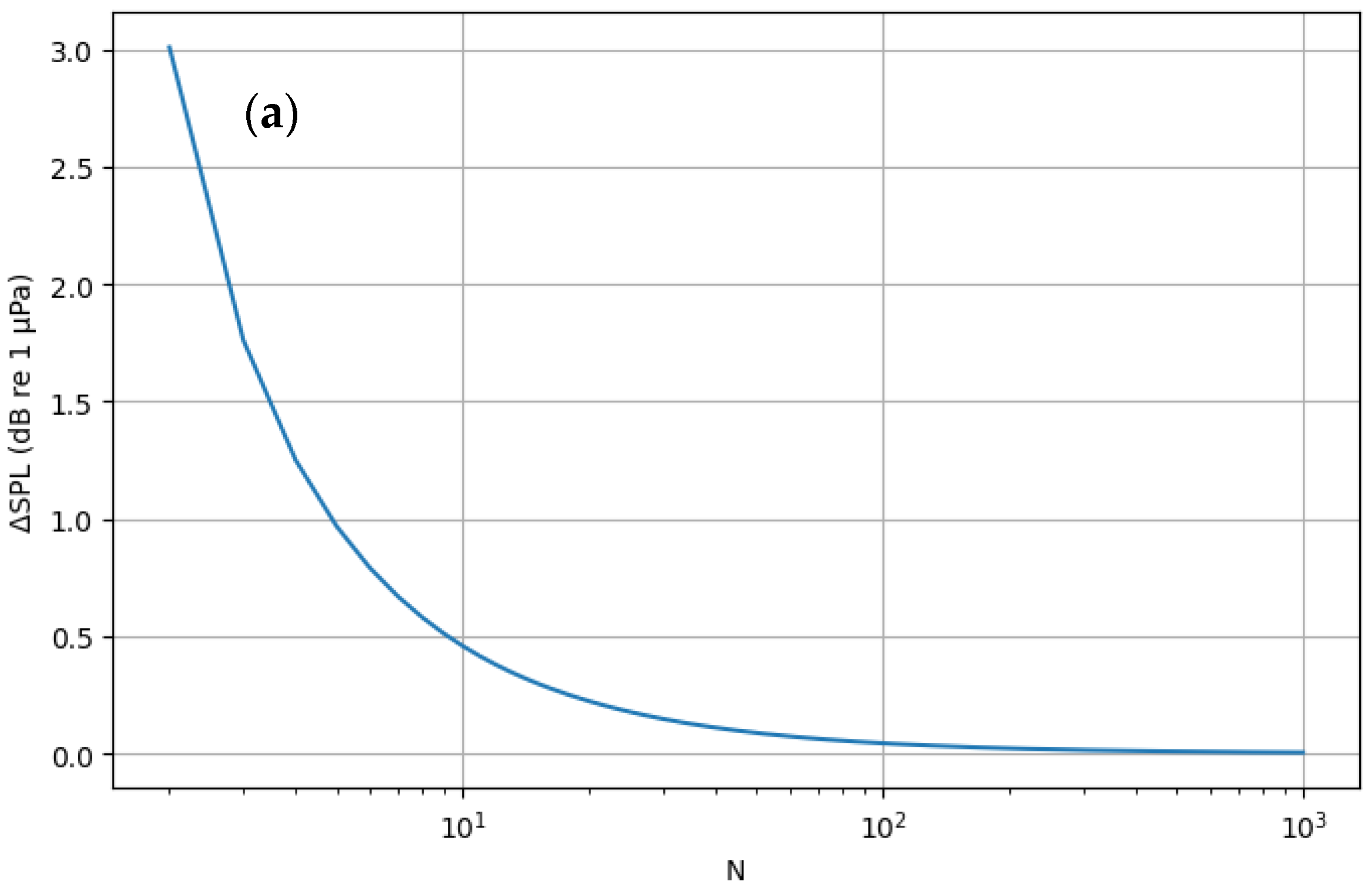
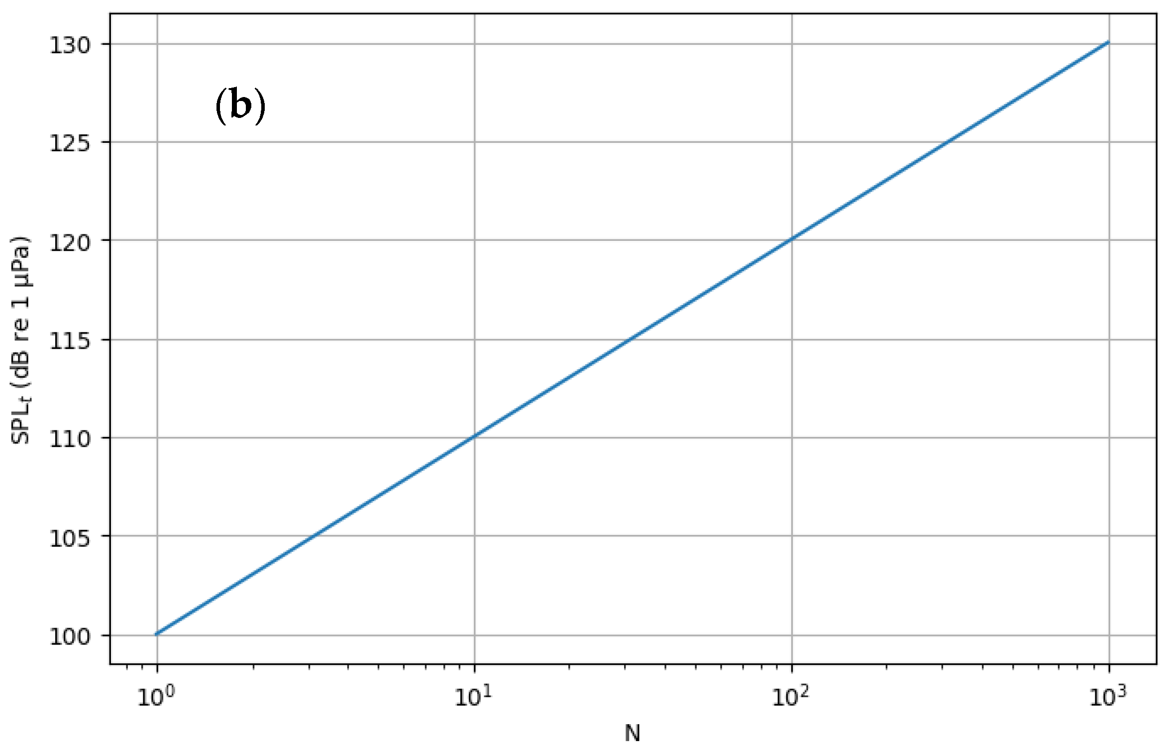
This result shows that the additional contribution of each new source (from N = 2 onward) is independent of the absolute SPL₀ of a single source, and decreases monotonically as N increases. Figure 8a illustrates ΔSPL(N) as a function of N. The trend highlights that the relative effect of each new turbine diminishes rapidly: for instance, once 10 turbines are already present, adding one more increases the overall level by less than 0.5 dB. Figure 8b shows the total SPL (SPL_t) from N sources of SPL₀ = 100 dB re 1 μPa.

Figure 8. (a) Incremental SPL (ΔSPL) of the N-th source, assuming all sources have the same SPL. (b) Total SPL (SPL_t) obtained by adding N sources, each with an SPL of 100 dB re 1 μPa.

3.2. Single Turbine Noise Spectrum

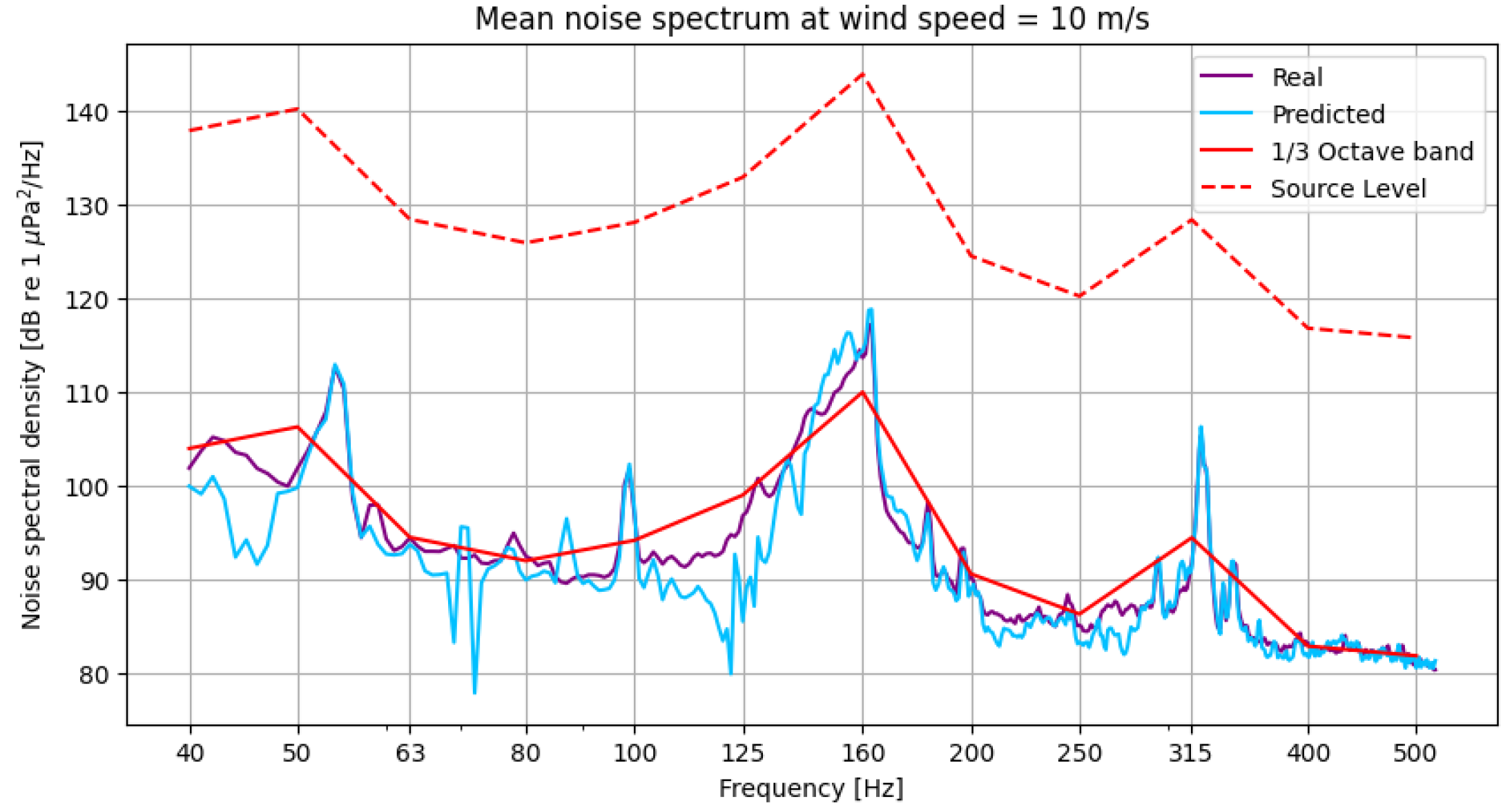
The measured and predicted noise spectra of a single turbine operating at 10 m/s exhibit three dominant peaks at 50, 160, and 315 Hz (Figure 9). This wind speed produces the strongest tonal peak, centered at 160 Hz, among the wind speeds that generate the most energetic spectrum. Although higher wind speeds generate slightly higher tonal peaks (up to 2 db re 1 μPa² at 160 Hz), they are associated with lower broadband energy. In contrast, wind speeds of 7–9 m/s show higher broadband energy than 10 m/s, but with a significantly weaker 160 Hz peak (see Supplementary Materials, section D).

Figure 9. Real (purple) and predicted (blue [3]) noise spectral density (dB re 1 μPa²/Hz) from a single turbine located 50 m away, operating at a wind speed of 10 m/s. Red lines indicate the one-third octave band SPL from the real spectrum at 50 m (solid line) and at 1 m from the source (dashed line; source level).

In this study, the real spectrum was used for analysis, as the predicted spectrum may vary between runs. For computational efficiency, one-third octave bands were back-propagated to the source (50 m), assuming spherical spreading.

In Figure 9, units differ between representations: noise spectral density is expressed in dB re 1 μPa²/Hz, whereas one-third octave band SPL-s are in dB re 1 μPa. Note that the highest noise occurs at 160 Hz, where the SL reaches 143 dB re 1 μPa.

3.3. OWF Noise Aggregated SPL Effect Simulation

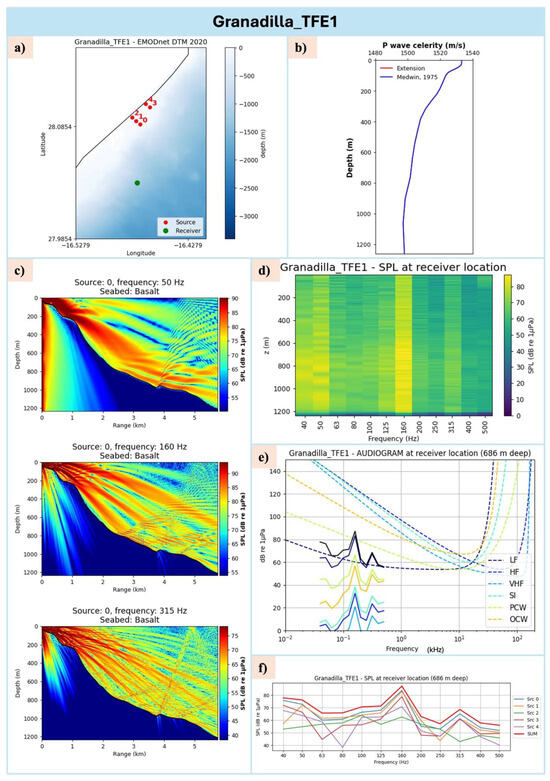
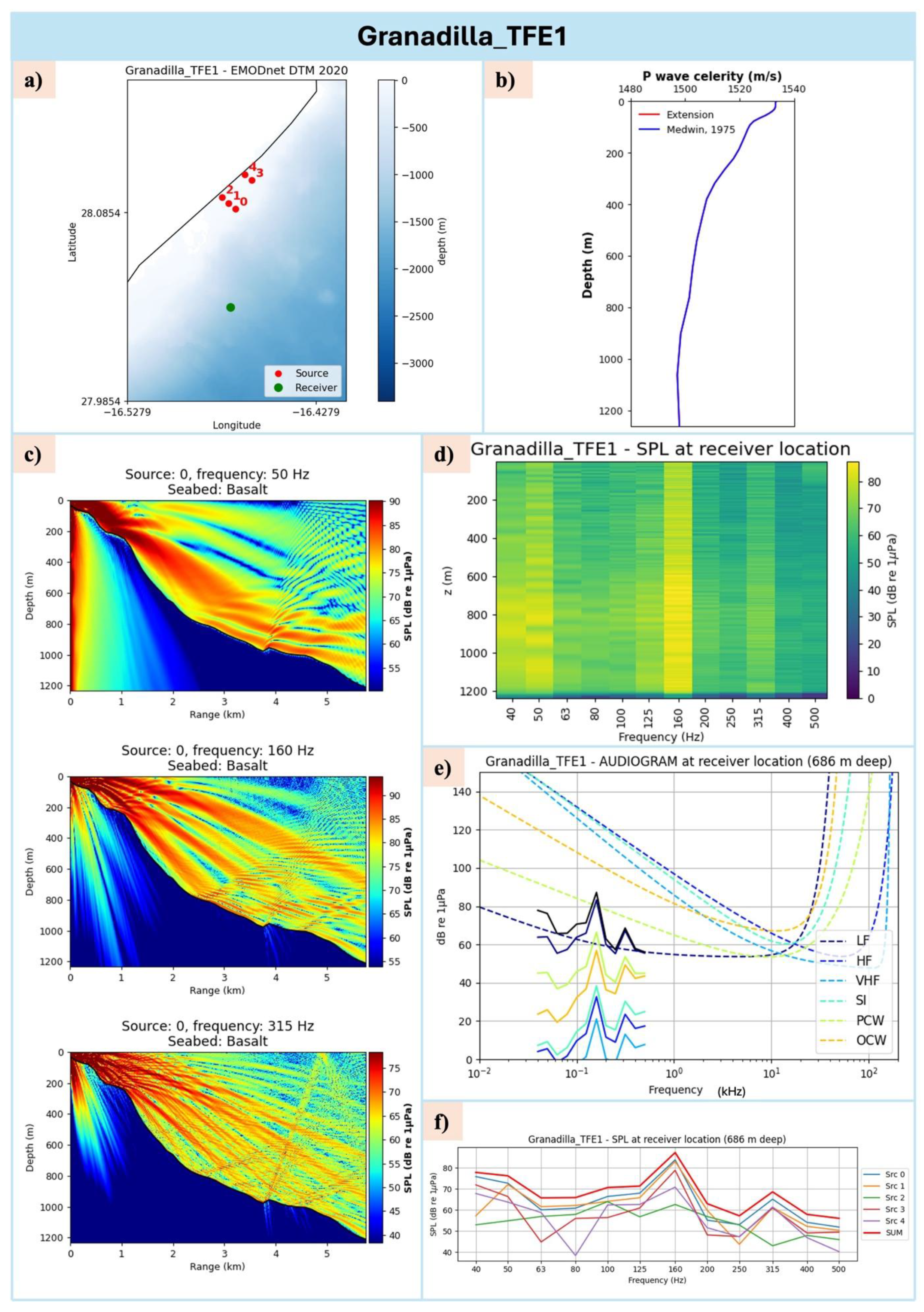
We present the main outputs from each OWF to each receiver section in the Supplementary Materials, section E. As an example, Figure 10 provides the description of the outputs obtained with this software.

Figure 10. Example of the main outputs from each offshore wind farm (OWF) to its respective receiver (in this case, Granadilla → TFE1). (a) Bathymetry map of the analyzed OWF and the receiver area. (b) Deepest sound speed profile between Source 0 and the receiver. (c) Source 0 to receiver SPL sections at specified frequency peaks: 50, 160, and 315 Hz. (d) SPL spectrum across depth at the receiver location (color indicates SPL). (e) Continuous lines: Weighted SPL spectra at the depth of maximum sound level for each auditory group (colors correspond to the legend). Dashed lines: Audiograms of the respective groups. (f) SPL spectra at the depth of maximum sound level for each source individually (thin lines) and the cumulative spectrum of all sources (thick red line). Figures for all sections are provided in the Supplementary Materials.

Key insights from the multiple OWF–receiver analyses (Supplementary Materials, Section E) highlight the influence of seabed type and topography on noise transmission, as well as the biological relevance of combined SPL from multiple turbines. Basalt seabeds (Granadilla and Tarahal OWFs) exhibit lower transmission losses along the seafloor, with sound reflecting toward the surface, whereas chalk seabeds (PEI and N10.2 OWFs) produce higher losses, particularly at low frequencies (See Supplementary Materials, section E, Granadilla_TFE1 and PEI_INP, Panel c). Steep or mountainous seabeds further increase low-frequency transmission losses (Supplementary Materials, section E, PEI_BE, PEI_FR, PEI_NL, Panel c). Regarding biological implications, within OWFs, weighted SPLs exceed audiogram thresholds for both Low-Frequency cetaceans (LF) and Phocid Carnivores in Water (PCW), while outside OWFs, only LF species are significantly affected (Table 2, Thresholds crossed; Supplementary Materials, section E, e Panels). Finally, the combined SPL from multiple turbines compared to a single turbine can raise SPLs by up to 10 dB (N10.2), with the largest contribution consistently coming from the turbine closest to the receiver (Supplementary Materials, section E, f Panels). However, the relative effect of adding further turbines diminishes as their number increases.

Table 2. Summary of propagation model outputs for each OWF at each receiver. Column 1 lists the OWF ID and number of turbines; Column 2 lists the receiver ID. Avg range indicates the average distance between OWF turbines and the receiver. Max depth is the maximum bathymetric depth along the path from turbines to receiver, while Rec depth denotes the bathymetric depth at the receiver. Max SPL depth is the depth where the aggregated SPL spectrum is most intense at the receiver. Max SPL represents the combined SPL from all turbines at each peak frequency at the receiver location and max SPL depth. Thresholds crossed indicate the auditory groups predicted to be affected by OWF noise aggregated across turbines at each receiver location and corresponding max SPL depth.

						max SPL (dB re 1 uPa)
OWF ID (# Turbines)	Receiver ID	Avg Range (km)	Max Depth (m)	Rec Depth (m)	Max SPL Depth (m)	50 Hz	160 Hz	315 Hz	Thresholds Crossed
Granadilla 5	ING	1.05	46.4	46.2	26	101.08	109.16	90.77	LF/PCW
	TFE1	6.73	1211.6	1211.6	686	76.21	87.24	68.60	LF
	TFE2	52.88	2159.6	2159.6	1614	58.97	65.33	44.15	LF
	GC1	60.97	2539.8	87.6	56	70.62	74.35	56.24	LF
Tarahal 15	INT	2.71	500.2	322.2	60	96.93	102.43	82.32	LF/PCW
	GC2	30.92	500.2	59.2	38	71.39	83.99	64.65	LF
	GC3	24.16	500.2	31.2	28	77.04	86.48	66.68	LF
	GC4	7.64	500.2	54.4	4	81.58	98.96	77.97	LF
	FTV1	81.04	2008.2	28.4	26	81.72	78.21	62.06	LF
	FTV2	100.82	2046.4	65.8	12	60.38	57.51	40.38	LF
PEI 15	INP	2.6	38.88	33.1	9	104.51	109.65	91.80	LF/PCW
	BE	44.70	40.17	12.45	7	5.51	79.21	68.33	LF
	FR	104.80	60.1	49.45	16	23.04	62.86	43.41	-
	NL	49.73	68.79	15.97	11	59.49	80.56	65.23	LF
N10.2 16	INN	2.48	41.54	40.57	39	107.20	112.15	96.04	LF/PCW
	DE1	82.90	41.54	25.68	15	63.65	80.56	65.33	LF
	DE2	81.16	41.53	24.2	16	65.33	81.44	64.47	LF
	NL2	165.79	48.47	39.15	30	52.64	71.84	58.72	LF
	NL3	206.10	49.3	38.08	29	44.19	67.66	53.27	LF

We synthesize the most relevant results in Table 2 to have a broad perspective of the implications of the aggregated effect from the OWF turbines on the different.

From Table 2, several conclusions emerge regarding noise levels inside (INX receivers) and outside OWFs. Inside the farms, the SPL reaches 100 dB in almost all sections at all peak frequencies (50, 160, and 315 Hz). Outside the farms, SPL attenuation varies with distance depending on bathymetry, sound speed profile, and sediment type: the lowest level (5.51 dB re 1 µPa at 50 Hz) occurs at 44.7 km in the PEI_BE section, while the highest (98.96 dB re 1 µPa at 160 Hz) is found at 7.6 km in the Tarahal_GC4 section.

Audiogram comparisons indicate that, inside OWFs, weighted spectra exceed the hearing thresholds for both Low-Frequency (LF) cetaceans and Phocid Carnivores in Water (PCW), whereas outside the OWFs, only LF species’ audiograms are crossed, as highlighted in the previous section. Table 3 presents the NMFS harassment criteria [11] compared to the values from our study. The 24 h aggregated weighted sound exposure level (L_{E,p,X,24 h}, where X refers to the relevant auditory group) remains below the threshold in all cases, indicating that no species would suffer auditory injury. In contrast, the B Harassment criterion’s root mean square SPL (L_p,RMS) threshold for continuous noise is exceeded inside all OWFs, with the exception of Tarahal, indicating potential behavioral harassment at the ING, INP, and INN receiver locations.

Table 3. 24 h aggregated weighted sound exposure level (L_{E,p,X,24 h}) for each source–receiver section, presented together with the corresponding NMFS A-harassment thresholds for each auditory group (LF and PCW). The final column reports the root mean square SPL (L_p,RMS) for each section, along with the NMFS B-harassment threshold for continuous noise.

			Level A Harassment						Level B Harassment
			LE,p,X,24 h (dB re 1 µPa2 s)						Lp,RMS (dB re 1 µPa)
			LF	HF	VHF	SI	PCW	OCW	Continuous
OWF ID	Receiver ID	Avg Range (km)	197	201	181	-	195	199	120
Granadilla	ING	1.05	170.71	121.25	110.05	127.33	154.19	145.95	125.56
	TFE1	6.73	148.75	99.29	88.09	105.37	132.23	123.99	103.47
	TFE2	52.88	126.68	76.59	65.13	82.42	109.98	100.99	81.56
	GC1	60.97	136.07	86.72	75.58	92.86	119.56	111.48	91.35
Tarahal	INT	2.71	163.95	114.31	103.05	120.34	147.36	138.94	118.90
	GC2	30.92	145.46	95.97	84.75	102.03	128.92	120.65	100.09
	GC3	24.16	147.93	98.39	87.15	104.43	131.38	123.04	102.60
	GC4	7.64	160.36	110.67	99.39	116.67	143.77	135.25	114.95
	FTV1	81.04	140.53	91.02	79.87	97.15	123.95	115.81	97.02
	FTV2	100.82	119.80	70.05	58.84	76.12	103.13	94.76	76.63
PEI (Princess Elisabeth I)	INP	2.6	171.35	122.21	111.12	128.40	154.91	147.05	126.23
	BE	44.70	141.87	94.89	84.24	101.50	126.29	120.30	95.92
	FR	104.80	124.27	74.78	63.55	80.83	107.74	99.44	78.77
	NL	49.73	142.39	93.82	82.84	100.11	126.17	118.82	96.78
N10.2	INN	2.48	173.91	124.80	113.68	130.96	157.50	149.64	128.85
	DE1	82.90	142.51	93.91	82.93	100.20	126.28	118.91	96.96
	DE2	81.16	143.22	94.59	83.67	100.93	126.94	119.59	97.71
	NL2	165.79	134.02	85.75	74.80	92.07	117.94	110.83	88.33
	NL3	206.10	129.65	81.29	70.36	87.63	113.51	106.36	84.01

4. Discussion

The propagation of OWF noise varies widely depending on bathymetry, seabed sediment, the water column sound speed profile, and turbines’ geographical distribution. Consequently, the same noise signal can behave very differently in distinct marine environments. This variability aligns with previous findings showing that seabed composition and bathymetry significantly alter low-frequency sound propagation [21,22]. Therefore, obtaining accurate estimates of the environmental variables influencing the propagation model is essential to reliably assess potential acoustic impacts. In this study, several assumptions were made to address data gaps, always adopting a conservative approach. The analysis focused on the 40–500 Hz frequency range, where operational wind turbine noise is most relevant and overlaps with the hearing range of several marine mammal groups [2].

While the theoretical analysis shows that adding turbines with identical source levels (SLs) located at the same site leads to diminishing acoustic gains—less than 0.5 dB re 1 µPa beyond approximately ten turbines—this finding should be interpreted in context. Tougaard et al. emphasize that, despite the limited local increase in SPL, the cumulative contribution from the growing number and size of OWFs can become considerable when assessed on a broader spatial scale [23]. As more turbines are deployed over increasingly large areas, the likelihood that vulnerable species will occur in proximity to at least one turbine also increases. Given that distance is the key factor influencing received SPL, the expansion of OWFs across wider regions effectively enlarges the area exposed to potentially harmful noise levels, thereby amplifying the overall ecological risk.

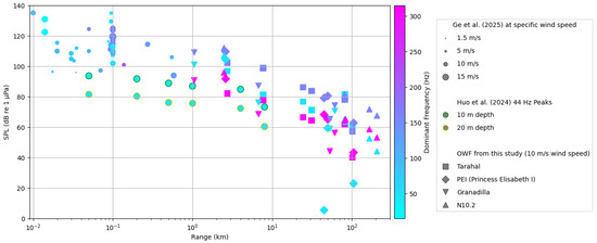
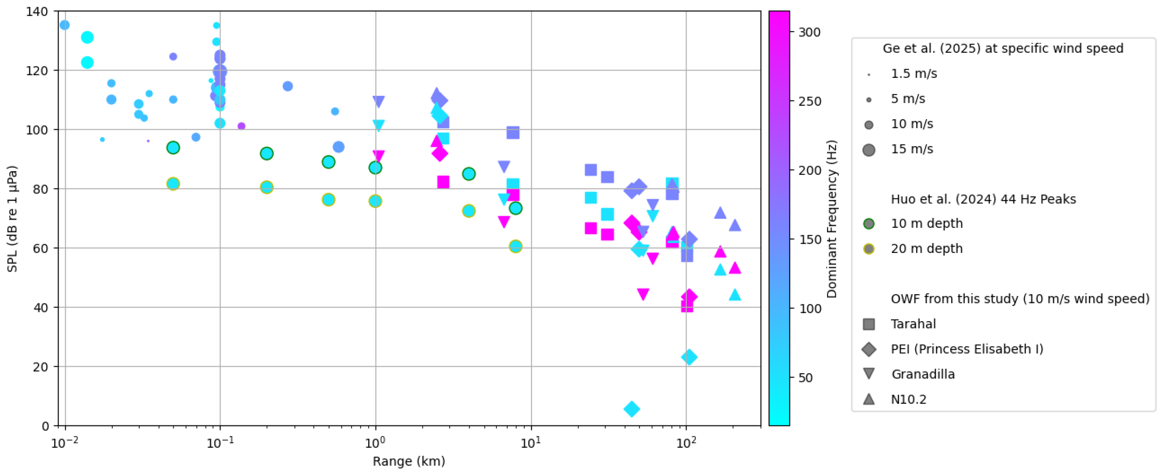
The main operational noise of the OWF at a wind speed of 10 m/s is centered at 160 Hz within the one-third octave band, with a single turbine producing an SL of up to 143 dB in this frequency band. Several studies have measured or propagated operational OWF noise data. Figure 11 compares the results from this study with published OWF data [22,24], presenting SPL as a function of range, frequency, and wind speed (for [24]). At 160 Hz (purple line), corresponding to 10 m/s wind speed, the decay is approximately linear, and the SPL values from our study align well with those reported by [24]. At lower frequencies, however, results are more heterogeneous, reflecting greater variability in transmission losses due to differences in environmental and geoacoustic characteristics [23]. Ref. [22] reported a fundamental frequency of 44 Hz from gear meshing, with the highest SPL associated with this frequency in fixed-based monopile turbines in the shallow waters of Yangjiang OWF. The SPL values reported by Huo et al. at measurement depths of 10 and 20 m were 2–10 dB lower (re 1 μPa) than the SPL observed in this study at 50 Hz, highlighting site-specific and structural differences in noise propagation.

Figure 11. Comparison of OWF SPL (y-axis) from our study with values from [22,24], as a function of range (x-axis), frequency (color), wind speed (marker size), and OWF (marker type).

Comparing the modeled SPLs within North Sea OWFs with published ambient noise measurements [12] enables an assessment of the relative contribution of OWF noise to the existing soundscape at the PE-I and N-10.2 sites. At site 08-BE-WST (21 m depth), located near the PE-I OWF, ambient RMS 1/3-octave SPLs between 50 and 300 Hz range from ~110 to 120 dB re 1 μPa, exceeding the modeled OWF noise levels. This area is characterized by intense marine traffic due to its proximity to the English Channel, suggesting that OWF noise would be largely masked by the high ambient background. Similarly, near the N-10.2 OWF, ambient noise levels at site 06-DE-FN1 (33.9 m depth) are approximately 105–115 dB re 1 μPa, comparable to the modeled OWF SPLs and therefore likely only marginally perceptible. In contrast, ambient noise data are unavailable for the Canary region; consequently, canonical ambient noise curves [13] were used for reference. Under this assumption, the simulated SPLs at the OWF receiver locations (ING and INT) exceed heavy marine traffic noise levels at the dominant frequencies, yielding signal-to-noise ratios of approximately 20–25 dB re 1 μPa. Nevertheless, this comparison remains approximate, and site-specific ambient noise measurements are required to robustly assess the potential ecological implications of OWF noise in Canary waters.

Simulated SPLs exceed the auditory thresholds of Low-Frequency (LF) cetaceans and Phocid Carnivores in Water (PCW) [2], indicating that OWF noise would be audible by this species. NMFS recommended thresholds for marine mammals [11] suggest that no auditory injury would occur in the analyzed areas. However, the behavioral harassment threshold of 120 dB would be exceeded inside the OWFs, potentially affecting the distribution of marine mammals and associated ecosystems in nearby regions.

Overall, these findings highlight the complexity of predicting underwater acoustic fields from OWFs and reinforce the need for site-specific, interdisciplinary assessments. Future research should focus on three key areas. First, improved characterization of environmental parameters—such as bathymetry, sediment type, and sound speed profiles—is essential to refine and validate propagation models. Second, more detailed knowledge of species distribution, hearing thresholds, and behavioral sensitivities is needed to accurately assess potential biological impacts. Third, the development of effective mitigation and monitoring strategies, including an effective characterization of background noise in areas with lack of data, should accompany OWF planning and operation to minimize acoustic disturbance. Integrating these components through combined modeling, in situ acoustic measurements, and ecological monitoring will enhance the reliability of impact assessments and support sustainable offshore wind development.

5. Conclusions

This study demonstrates that the propagation of underwater noise from offshore wind farms (OWFs) is highly site-specific, influenced by bathymetry, seabed composition, sound speed profiles, and turbine distribution. Modeled SPLs align well with published measurements at key frequencies but reveal substantial variability at lower frequencies, reflecting environmental and structural differences across sites. Sensitivity analyses indicate that variations in wind speed could enhance the SL noise spectral density 160 Hz peak by 2 dB re 1 µPa²/Hz, while differences in sediment type can lead to transmission loss variations ranging could rise up 100 dB, depending on bathymetry and range. We adopted conservative values in all cases. While single-turbine contributions to local SPL diminish rapidly beyond ten turbines, the cumulative effect of expanding OWFs across broader regions increases the spatial area exposed to potentially audible noise, particularly for low-frequency cetaceans and phocid carnivores. Comparison with ambient noise levels suggests that OWF noise is often masked in high-traffic areas, though it may be more prominent in regions with lower background noise, such as the Canary Islands. No risk of auditory injury is expected, yet behavioral disturbance thresholds could be exceeded within OWF boundaries, with possible ecological implications. These results highlight the importance of site-specific acoustic characterization, refined propagation modeling, and ecological monitoring. Future research should prioritize accurate environmental parameterization, improved understanding of species’ auditory and behavioral responses, and the development of effective mitigation strategies to ensure sustainable offshore wind development with minimal acoustic impact.

References

- Wahlberg, M.; Westerberg, H. Hearing in fish and their reactions to sounds from offshore wind farms. Mar. Ecol. Prog. Ser. 2005, 288, 295–309. [Google Scholar] [CrossRef] [Scilit]
- Southall, B.L.; Finneran, J.J.; Reichmuth, C.; Nachtigall, P.E.; Ketten, D.R.; Bowles, A.E.; Ellison, W.T.; Nowacek, D.P.; Tyack, P.L. Marine mammal noise exposure criteria: Updated scientific recommendations for residual hearing effects. Aquat. Mamm. 2019, 45, 125–232. [Google Scholar] [CrossRef] [Scilit]
- Trucco, A. Predicting underwater noise spectra dominated by wind turbine contributions. IEEE J. Ocean Eng. 2024, 49, 1675–1694. [Google Scholar] [CrossRef] [Scilit]
- Collins, M.D. User’s Guide for RAM Versions 1.0 and 1.0p; Naval Research Laboratory: Washington, DC, USA, 1995; Available online: https://oalib-acoustics.org/website_resources/PE/RAM.pdf (accessed on 15 November 2024).
- Porter, M.B. The BELLHOP Manual and User’s Guide: Preliminary Draft; Heat, Light, and Sound Research, Inc.: La Jolla, CA, USA, 2011; Available online: http://oalib.hlsresearch.com/Rays/HLS-2010-1.pdf (accessed on 4 November 2025).
- El Día. El Primer Parque Eólico Marino de Tenerife Empezará a Construirse en 2024. 13 December 2023. Available online: https://www.eldia.es/tenerife/2023/12/13/primer-parque-eolico-marino-tenerife-95815226.html (accessed on 4 November 2025).
- Parque Tarahal. Documentos del Proyecto. Available online: https://parquetarahal.com/documentos/ (accessed on 17 July 2025).
- Federal Public Service Economy. Identification of the Parcels for the Construction of Wind Farms in the Belgian North Sea. Available online: https://economie.fgov.be/en/themes/energy/sources-and-carriers-energy/offshore/tenders/identification-parcels (accessed on 23 July 2025).
- OffshoreWIND.biz. Germany Marks Two Areas as Suitable for 2.5 GW Offshore Wind. OffshoreWIND.biz. 28 January 2025. Available online: https://www.offshorewind.biz/2025/01/28/germany-marks-two-areas-as-suitable-for-2-5-gw-offshore-wind/ (accessed on 4 November 2025).
- European Environment Agency. Natura 2000 Data: The European Network of Protected Sites. Available online: https://natura2000.eea.europa.eu/ (accessed on 1 September 2025).
- NMFS (National Marine Fisheries Service). Summary of Recommended Marine Mammal Protection Act Acoustic Thresholds; NMFS, Office of Protected Resources: Silver Spring, MA, USA, 2025. [Google Scholar]
- Basan, F.; Fischer, J.-G.; Putland, R.; Brinkkemper, J.; De Jong, C.A.F.; Binnerts, B.; Norro, A.; Kühnel, D.; Ødegaard, L.-A.; Andersson, M.; et al. The underwater soundscape of the North Sea. Mar. Pollut. Bull. 2024, 198, 115891. [Google Scholar] [CrossRef] [Scilit] [PubMed]
- Wenz, G.M. Acoustic ambient noise in the ocean: Spectra and sources. J. Acoust. Soc. Am. 1962, 34, 1936–1956. [Google Scholar] [CrossRef] [Scilit]
- Hersbach, H.; Bell, B.; Berrisford, P.; Hirahara, S.; Horányi, A.; Muñoz-Sabater, J.; Nicolas, J.; Peubey, C.; Radu, R.; Schepers, D.; et al. The ERA5 global reanalysis. Q. J. R. Meteorol. Soc. 2020, 146, 1999–2049. [Google Scholar] [CrossRef] [Scilit]
- Davis, N.N.; Badger, J.; Hahmann, A.N.; Hansen, B.O.; Mortensen, N.G.; Kelly, M.; Larsén, X.G.; Olsen, B.T.; Floors, R.; Lizcano, G.; et al. The Global Wind Atlas: A high-resolution dataset of climatologies and associated web-based application. Bull. Am. Meteorol. Soc. 2023, 104, E1507–E1525. [Google Scholar] [CrossRef] [Scilit]
- OffshoreWIND.biz. Belgium Delays Tender for Offshore Wind Farm in Princess Elisabeth Zone Until 2026. OffshoreWIND.biz. 1 July 2025. Available online: https://www.offshorewind.biz/2025/07/01/belgium-delays-tender-for-offshore-wind-farm-in-princess-elisabeth-zone-until-2026/ (accessed on 4 November 2025).
- GRAFCAN/Gobierno de Canarias. Visor IDECanarias. Available online: https://visor.grafcan.es/ (accessed on 11 September 2025).
- Thierry, S.; Dick, S.; George, S.; Benoit, L.; Cyrille, P. EMODnet Bathymetry: A compilation of bathymetric data in the European waters. In Proceedings of the OCEANS, Marseille, France, 17–20 June 2019; pp. 1–7. [Google Scholar] [CrossRef] [Scilit]
- Medwin, H. Speed of sound in water: A simple equation for realistic parameters. J. Acoust. Soc. Am. 1975, 58, 1318–1319. [Google Scholar] [CrossRef] [Scilit]
- GLOBAL_MULTIYEAR_PHY_001_030 Global Ocean Physics Reanalysis, E.U. Copernicus Marine Service Information (CMEMS), Marine Data Store (MDS). Available online. (accessed on 6 June 2025). [CrossRef]
- Godin, O.A. Underwater sound propagation over a layered seabed with weak shear rigidity. J. Acoust. Soc. Am. 2025, 157, 314–327. [Google Scholar] [CrossRef] [Scilit] [PubMed]
- Huo, X.; Zhang, P.; Feng, Z. Study of underwater sound propagation and attenuation characteristics at the Yangjiang offshore wind farm. Ecol. Inform. 2024, 84, 102919. [Google Scholar] [CrossRef] [Scilit]
- Tougaard, J.; Hermannsen, L.; Madsen, P.T. How loud is the underwater noise from operating offshore wind turbines? J. Acoust. Soc. Am. 2020, 148, 2885–2893. [Google Scholar] [CrossRef] [Scilit] [PubMed]
- Ge, Q.; Yao, H.; Qian, S.; Zhang, X.; Guo, H. Dependencies of Underwater Noise from Offshore Wind Farms on Distance, Wind Speed, and Turbine Power. Acoustics 2025, 7, 71. [Google Scholar] [CrossRef] [Scilit]
- Donnelly, M. pyRAM: Python Adaptation of the Range-Dependent Acoustic Model (RAM). PyPI. 2017. Available online: https://pypi.org/project/pyram/ (accessed on 6 June 2025).
- Porter, M.B. The BELLHOP Acoustic Ray Tracing Model. HLS Research. 2005. Available online: http://oalib.hlsresearch.com/AcousticsToolbox/ (accessed on 6 June 2025).
- Chitre, M. Arlpy: Acoustic Research Laboratory Python Library. GitHub. 2020. Available online: https://github.com/org-arl/arlpy/ (accessed on 6 June 2025).
- Copernicus Marine Service. Copernicus Marine Toolbox API–Subset. Copernicus Marine Service. 2024. Available online: https://help.marine.copernicus.eu/en/articles/8283072-copernicus-marine-toolbox-api-subset (accessed on 6 June 2025).
- EDDAPY. Python Client for Accessing ERDDAP Servers. PyPI. 2023. Available online: https://pypi.org/project/erddapy/ (accessed on 6 June 2025).
- Hamilton, E.L. Geoacoustic modeling of the sea floor. J. Acoust. Soc. Am. 1980, 68, 1313–1340. [Google Scholar] [CrossRef] [Scilit]
- Jensen, F.B.; Kuperman, W.A.; Porter, M.B.; Schmidt, H. Computational Ocean Acoustics, 2nd ed.; Springer: New York, NY, USA, 2011. [Google Scholar] [CrossRef] [Scilit]
- Pangerc, T.; Theobald, P.D.; Wang, L.S.; Robinson, S.P.; Lepper, P.A. Measurement and characterisation of radiated underwater sound from a 3.6 MW monopile wind turbine. J. Acoust. Soc. Am. 2016, 140, 2913–2922. [Google Scholar] [CrossRef] [Scilit] [PubMed]
Disclaimer/Publisher’s Note: The statements, opinions and data contained in all publications are solely those of the individual author(s) and contributor(s) and not of MDPI and/or the editor(s). MDPI and/or the editor(s) disclaim responsibility for any injury to people or property resulting from any ideas, methods, instructions or products referred to in the content. |
© 2025 by the authors. Licensee MDPI, Basel, Switzerland. This article is an open access article distributed under the terms and conditions of the Creative Commons Attribution (CC BY) license.