A U-Net-Based Prediction of Surface Pressure and Wall Shear Stress Distributions for Suboff Hull Form Family

Abstract

Recent developments in machine learning have enabled prediction models that estimate not only hydrodynamic force coefficients but also full CFD fields. Unlike conventional surrogate models that focus primarily on integrated quantities, such approaches can provide real-time predictions of pressure and wall shear stress distributions, making them highly promising for applications in ship hydrodynamic design where detailed surface flow characteristics are essential. In this study, we address the low prediction accuracy observed near protruding appendages in U-Net-based field prediction models by introducing a positional encoding (PE)-enhanced data processing scheme and evaluating its performance across a dataset of 500 SUBOFF variants. While PE enhances prediction accuracy, especially for the sail, its effectiveness is constrained by the boundary discontinuity introduced at the 12 o’clock seam. To resolve this structural limitation and ensure consistent accuracy across components, the projection seam is relocated to the 6 o’clock position, where high-gradient flow features are less concentrated. This modification produces clear quantitative gains: the drag-integrated MAPE decreases from 3.61% to 1.85%, and the mean field-level errors of $∆{\mathrm{C}}_{\mathrm{p}}$ and $∆{\mathrm{C}}_{\mathrm{f}}$ are reduced by approximately 5.6% across the dataset. These results demonstrate that combining PE with seam relocation substantially enhances the model’s ability to reconstruct fine-scale flow features, improving the overall robustness and physical reliability of U-Net-based surface field prediction for submarine hull forms.

1. Introduction

For submerged submarines, hydrodynamic resistance is a primary performance indicator directly related to propulsive efficiency, energy consumption, noise and vibration characteristics, and overall operational economics. In geometrically complex arrangements—comprising the hull, sail, and multiple rudders—appendage-level modifications can substantially alter pressure and wall shear stress distributions, with commensurate effects on resistance (Saghi, Parunov & Mikulić [1]). Consequently, in the context of design automation and multi-objective optimization, approaches that shorten the shape design–analysis–evaluation loop while maintaining predictive fidelity are of critical importance.

Traditionally, Reynolds-Averaged Navier–Stokes (RANS)-based computational fluid dynamics (CFD) has served as the standard approach for resistance prediction. However, during the design space exploration stage—where high-resolution meshes, detailed boundary-layer treatment, and numerous shape variation cases are considered—CFD alone often cannot deliver sufficient speed and coverage. In this context, physics-informed neural networks have emerged to embed governing constraints into learning for reliable flow prediction (Raissi et al. [2]), and comprehensive reviews show that machine learning is increasingly used for sustainable ship design and operation (Huang [3]). Consequently, recent studies have actively explored submarine resistance prediction using data-driven artificial neural networks to complement or, in part, replace physics-based analyses (Wu et al. [4]; X. Chu et al. [5]; Guo et al. [6]). Among multi-fidelity approaches, a U-Net model has been shown to reconstruct high-fidelity viscous fields from low-fidelity inviscid simulations around ship hulls, highlighting an effective path for rapid yet accurate field recovery (Kim et al. [7]).

In addition to these developments, several very recent studies from 2024 to 2025 have further expanded machine learning applications for SUBOFF hydrodynamics. Hao et al. [8] introduced a deep graph learning framework capable of rapidly predicting the wake field behind the DARPA SUBOFF model, demonstrating the effectiveness of graph-based neural architectures in capturing unstructured wake features. Alongside this work, the PINN-based resistance prediction by Wu et al. [4], the LBM–PINN flow reconstruction method of Chu et al. [5], and the spatio-temporal graph neural network proposed by Guo et al. [6] collectively highlight the accelerating trend toward data-driven surrogate modeling for submarine flow analysis. However, these approaches largely focus on global resistance coefficients, wake characteristics, or pressure-only field reconstruction for a single reference geometry. They do not address the simultaneous prediction of surface pressure (${\mathrm{C}}_{\mathrm{p}}$) and wall shear stress (${\mathrm{C}}_{\mathrm{f}}$) distributions across the main hull, sail, and rudders for a large family of geometrically perturbed submarine variants—a capability that is essential for practical design exploration and directly targeted in the present study.

However, due to the inductive bias of convolutions, pure convolutional neural networks (CNNs) are strongly translation-equivariant and relatively insensitive to absolute positional information. As a result, even when overall geometry is similar, they may fail to capture differences in pressure and wall shear distributions that arise from features appearing at different locations on the hull. In submarines, this limitation is pronounced near high-gradient regions—such as the junctions between the sail and the hull or around the rudders—where pure CNNs often exhibit degraded performance.

Building on the above motivation, this study proposes a U-Net-based submarine resistance prediction model that systematically aggregates hull form and CFD data and augments the network with positional encoding (PE). Concretely, using the DARPA SUBOFF as the baseline geometry, we generate diverse variants via free-form deformation (FFD) and compute surface pressure and wall shear distributions with CFD to construct the training set. The model input consists of per-part surface coordinates $(\mathrm{x},\mathrm{y},\mathrm{z})$, arranged as matrices on parameterized grids so that predictions can be mapped back to the original submarine surface after inference. Geometry features are extracted by the encoder, sinusoidal (sin/cos) positional encodings are injected to enrich absolute and relative positional cues, and the decoder outputs the coefficient fields—pressure coefficient $\left({\mathrm{C}}_{\mathrm{p}}\right)$ and skin friction coefficient $\left({\mathrm{C}}_{\mathrm{f}}\right)$.

Once trained, the network takes unseen geometric inputs and returns predicted ${\mathrm{C}}_{\mathrm{p}}$ and ${\mathrm{C}}_{\mathrm{f}}$ matrices, which are restored to the physical surface and integrated over the area to obtain the streamwise drag component. In this way, one can estimate the hydrodynamic drag acting on the submarine without running a new CFD simulation, enabling substantially faster and more cost-effective resistance prediction during design exploration.

2. Target Submarine Types

2.1. Reference Hull and Numerical Setup

The submarine considered in this study is the DARPA SUBOFF, and its hull form particulars in

Table 1. Hull form particulars of DARPA SUBOFF.

	Ship	Model
LOA	104.544 m	4.356 m
Max diameter	12.192 m	0.508 m
L/D	8.58
Scale	24

follow those reported by Groves et al. [9]. As shown in Figure 1, the DARPA SUBOFF features a cruciform empennage and consists of one sail and four rudders.

2.2. FFD-Based Variants of the Target Geometry

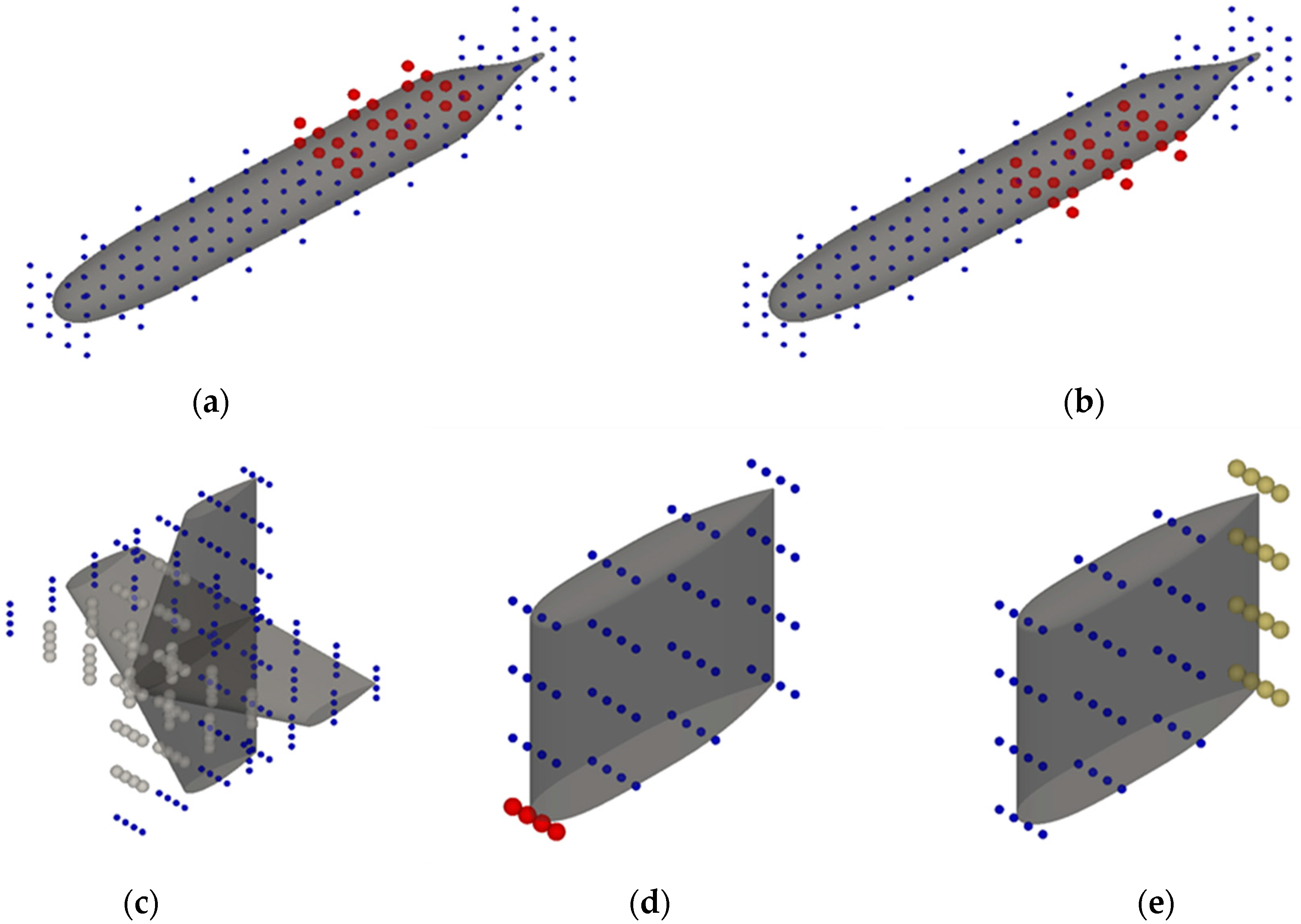
To train the neural network, we generated a total of 500 geometry cases by deforming the DARPA SUBOFF hull form using free-form deformation (FFD). Moreover, convolutional autoencoders were employed to learn hull form transformations directly from the geometric data, providing an unsupervised representation for shape variation (Seo et al. [10]). FFD enables smooth and global surface modification by displacing only the control points of an external control lattice. Some examples of hull form deformation used in this study are illustrated in Figure 2. In this study, the main hull was deformed with a lattice of $10\times 4\times 4$ control points along the x, y, and z directions, respectively (160 control points in total). Each appendage was deformed with a $4\times 4\times 4$ lattice (64 control points per appendage). The lattices for respective hull parts are presented in Figure 3.

2.2.1. Master Point

Master points are key control points selected for hull form modification such that when a master point is displaced, a prescribed neighborhood of points moves in concert. The nine master points and their corresponding deformation settings are summarized in

Table 2. Master point placement and deformation sites.

Master Point	Purpose
M1	Modify the forebody (bow) region
M2	Modify the lower afterbody (lower stern) region
M3	Modify the upper afterbody (upper stern) region
M4	Add filets to the rudders
M5	Add a filet at the sail–forebody junction
M6, M7	Apply an inclination (rake) modification to the sail’s afterbody
M8	Vary the sail position
M9	Adjust the forebody fullness (Nf)

.

2.2.2. Method for Determining Variation Magnitudes

To select the displacement magnitudes of the master points identified in Section 2.2.1, we employed Latin hypercube sampling (LHS), which provides a well-dispersed, non-overlapping design even with a relatively small sample size. Using this scheme, we generated 500 training cases by deforming the DARPA SUBOFF, imposing identical magnitude perturbations on the cruciform empennage in each case.

To ensure that the deformation space spanned by the nine master points (Table 2) was adequately explored, Latin hypercube sampling (LHS) was adopted as the design-of-experiments technique. LHS provides a stratified, space-filling sampling pattern in which the admissible range of each master point displacement is partitioned into N equiprobable intervals, with one sample selected from each interval. In this study, we generated $\mathrm{N}=500$ variants for $\mathrm{d}=9$ design variables, resulting in a sample-to-dimension ratio of ${\displaystyle \frac{\mathrm{N}}{\mathrm{d}}}\approx 55$, which satisfies and exceeds common guidelines for space-filling designs in engineering surrogate modeling.

The displacement bounds for each master point were selected to (i) avoid geometric infeasibility, such as surface overlap or detachment of appendages, and (ii) maintain hydrodynamically meaningful shape perturbations relative to the DARPA SUBOFF baseline. After generating the LHS samples in normalized space, each sample was mapped to its corresponding FFD. One- and two-dimensional projections of the samples were examined to verify that the design space was uniformly populated without clustering or voids. All resulting geometries were additionally inspected to confirm that no self-intersection occurred and that appendages remained properly connected.

Through these procedures, we verified that the chosen LHS parameters provide sufficient and well-balanced coverage of the SUBOFF hull form design space while maintaining computational feasibility for the required CFD simulations.

Moreover, because all training and test samples were drawn from the same bounded FFD design space, the present evaluation corresponds to an interpolative regime. The model was therefore validated within well-controlled geometric limits, leaving generalizations to substantially larger or extrapolative deformations for future investigations.

2.3. Governing Equations and Mesh System

The governing equations are those of incompressible turbulent flow, specifically, the continuity equation and the RANS momentum equations. Mesh generation and numerical simulations were conducted using STAR-CCM+ (ver. 15.06.008). A trimmed (Trimmer) mesh was employed, and to represent the boundary-layer flow on the hull with higher fidelity, a prism-layer technique was applied to generate 18 layers from the wall with a total thickness of 0.012 m. For turbulence modeling, the elliptic blending Reynolds stress model (ebRS) was selected. This model couples an elliptic blending equation with the RANS framework, provides a smooth treatment of near-wall effects, and is well suited to low-Reynolds-number integrations (e.g., low y⁺) without relying on wall functions. In this study, comparisons with model test data showed the best agreement under the low-y⁺, fully resolved boundary-layer setting; accordingly, the ebRS was adopted. The Reynolds number based on the SUBOFF length (4.356 m) and the inflow velocity of 6.17 m/s was approximately $Re =2.7\times {10}^7$, corresponding to a fully turbulent regime typical of submarine-scale flows.

Table 3. Domain size and boundary conditions.

Domain Size	−3.0 L < X < 3.0 L, −1.5 L < Y < 0, −1.5 L < Z < 1.5 L
Top	Symmetry plane
Bottom	Symmetry plane
Inlet	Velocity inlet
Outlet	Pressure outlet
Side	Symmetry plane

summarizes the domain size and boundary conditions adopted in the present CFD simulations.

To evaluate the flow fields for all FFD-generated variants, a consistent meshing strategy was applied across the entire dataset. A representative example, Case 5, is reported here to document mesh characteristics and near-wall resolution. The computational domain spans from −13.07 m to 13.07 m in the streamwise direction and ±6.53 m in the lateral and vertical directions. The resulting grid contains approximately 5.12 million control volumes, consisting of 14,417 tetrahedral cells, 4.32 million hexahedral cells, 586,992 wedge (prism) cells, 51 pyramids, and 195,572 polyhedral cells. The wetted surface of the SUBOFF geometry is resolved by 143,857 faces on the main hull and 4000–11,000 faces on each appendage, yielding a total wetted area of approximately 6.4 m². Mesh quality diagnostics indicate 100% face validity, no negative cell volumes, and a maximum boundary cell skewness angle below 86°, confirming that the grid is suitable for steady RANS simulations.

To ensure adequate boundary-layer resolution, 18 prism layers with a total thickness of 0.012 m were applied. For the representative Case 5, the dimensionless wall distance $y^{+}$ lies within the range $0.08\le y^{+}\le 5.85$ across all wetted surfaces (main hull, sail, and rudders). Because identical prism-layer parameters (first-layer height, number of layers, and growth rate) were used for all 500 variants, their $y^{+}$ distributions kept the same order of magnitude. Accordingly, the boundary layer was resolved predominantly within the viscous sublayer and buffer region for every case, enabling fully resolved low-$y^{+}$ treatment under the selected elliptic blending Reynolds stress (ebRS) turbulence model.

The choice of the elliptic blending Reynolds stress (ebRS) model is further justified by its suitability for flows exhibiting strong three-dimensional separation, curvature effects, and anisotropic stress structures around the sail and multiple rudders of the SUBOFF geometry. Unlike one- and two-equation eddy viscosity models such as the realizable k–ε, k–ω SST, or Spalart–Allmaras closures, Reynolds stress models (RSMs) solve transport equations for all components of the Reynolds stress tensor and therefore do not rely on the isotropy assumptions inherent to eddy viscosity formulations. This distinction is significant for the present configuration, where the interaction between the sail, appendages, and the main hull induces complex crossflow and non-equilibrium turbulence that is difficult to capture with eddy viscosity models. The elliptic blending formulation proposed by Manceau and Hanjalić [11] further improves the near-wall behavior of conventional RSMs through a smooth blending between wall-proximity and outer-flow turbulence structures, making it suitable for the fully resolved low-y⁺ treatment employed in this dataset. Accordingly, the ebRS model offers a favorable balance between predictive capability and computational tractability for generating high-fidelity pressure and wall shear stress fields over the 500 FFD-generated SUBOFF variants used in this study.

All simulations ran for the maximum iteration limit of 5000 steps. Variants that failed to reach stable residual reduction or exhibited oscillatory force behavior within this limit were categorized as divergent. In total, 99 cases fell into this category and were excluded, leaving 401 converged flow solutions for the final CFD dataset.

To assess the potential impact of excluding the diverged cases, we examined the characteristics of the 99 variants that did not reach convergence within the prescribed 5000 iterations. These cases do not cluster around a particular region of the LHS design space or exhibit systematic trends with respect to specific FFD control points or geometric features such as sail position, appendage filets, or forebody fullness. Instead, divergence generally occurred in scattered configurations where strong local separations developed at the junctions between the sail, rudders, and hull, occasionally leading to oscillatory forces or stagnating residuals. Since these diverged cases represent approximately 19.8% of the total 500 CFD runs and are broadly distributed across the parameter space, their exclusion does not introduce any identifiable geometric bias to the final dataset used for machine learning training.

Since all 500 CFD solutions were generated using a fully consistent RANS/ebRS configuration, the resulting training–validation split evaluates interpolation within a uniform numerical framework. As such, the present validation does not assess generalization to alternative CFD fidelities or solver settings, which is recognized as a limitation of the current dataset design.

Although symmetry planes are commonly used when only half of a geometrically symmetric body is modeled, full-domain simulations may also employ symmetry boundaries on lateral faces when the far-field boundaries are placed sufficiently far from the body. In the present setup, the domain extends ±1.5 L in the lateral and vertical directions, and preliminary tests confirmed that the pressure and wall shear distributions on the SUBOFF surface were insensitive to replacing symmetry planes with slip or far-field boundary conditions. Because the flow remains attached along most of the hull and the wake width is narrow relative to the domain height and width, reflective effects from the symmetry boundaries were found to be negligible at the distances selected here.

Nevertheless, we acknowledge that the use of symmetry planes may influence wake development in highly separated flows and could contribute to numerical sensitivity in some of the divergent cases. Future work will include additional tests using enlarged domains and alternative lateral boundary treatments to further assess the robustness of the CFD dataset.

2.4. Preprocessing of Hull Form Data for Training

For machine learning purposes, the submarine geometry was partitioned into six parts—the hull, the sail, and the four rudders—and each part was converted into a matrix representation suitable for input to a CNN. For every part, we prepared three matrices: (i) a geometry matrix encoding the shape information and (ii) two target matrices derived from STAR-CCM+ results, corresponding to the pressure-related and friction-related resistance fields (here represented as the pressure coefficient $C_p$ and skin friction coefficient $C_f$ distributions), as shown in Figure 4. Because the hull is larger and exhibits a more complex drag distribution, it was discretized to a 128 × 128 matrix, whereas the remaining parts were mapped to 64 × 64 matrices. Therefore, a single training instance comprises 18 matrices (six parts × three matrices per part). The geometry matrices serve as inputs to the network, and the $C_p$ and $C_f$ matrices are used as supervised outputs. To preserve geometric fidelity when mapping curved hull surfaces to image-like inputs for CNNs, curved-surface parameterizations tailored for wake/field prediction have also been proposed (Ichinose & Taniguchi, [12]).

The matrix resolutions adopted in this work—128 × 128 for the main hull and 64 × 64 for the sail and rudders—are consistent with established practices in machine learning-based flow-field reconstruction. Prior U-Net and CNN studies in turbulence super-resolution and RANS-level field prediction frequently employed 2D grids in the range of 64–256, with 128 × 128 emerging as a standard resolution balancing geometric fidelity and computational efficiency [13,14].

For marine applications, ship hull flow reconstruction research has shown that 128 × 128 grids for the primary hull surface and 64–96 grids for appendages are sufficient for preserving curvature and accurately reconstructing pressure- and shear-related fields [7]. Additionally, curved-surface projection methods for CNN field prediction indicate that resolutions around 128 × 128 maintain surface continuity without significant aliasing [12].

Recent SUBOFF-related surrogate modeling frameworks—such as deep graph wake prediction [8] and LBM-PINN-based flow reconstruction [5]—also utilize spatial representations within the 64–128 range, noting that further refinement yields diminishing returns relative to the increased computational burden. Because the projected pressure and wall shear distributions in our dataset are smoother than the original CFD mesh, additional resolution beyond 128 × 128 (main hull) and 64 × 64 (appendages) would not meaningfully improve learning accuracy.

Therefore, the selected resolutions represent an optimal compromise between geometric fidelity, predictive performance, and computational tractability, fully aligned with the existing literature.

3. Machine Learning

3.1. U-Net

To predict the spatial distributions of the pressure coefficient ${\mathrm{C}}_{\mathrm{p}}$ and skin friction coefficient ${\mathrm{C}}_{\mathrm{f}}$ on the submarine surface, we adopted a U-Net-type encoder–decoder structure. The encoder progressively reduces the spatial resolution to extract features representing the global geometry and layout, while the decoder restores the resolution to recover local details, thereby enabling simultaneous modeling of global context and fine-scale patterns. Relatedly, super-resolution reconstruction of turbulent flows from coarse inputs has demonstrated that CNN-based decoders can reliably recover fine-scale structures (Fukami et al. [13]).

The encoder consists of four consecutive blocks that progressively reduce spatial resolution, each containing two convolutional layers followed by a pooling operation. The number of filters decreases across the blocks of [128, 64, 32, 16]. A 3 × 3 kernel is used for all convolutions with ReLU activations. To preserve feature map dimensions after each convolution, zero-padding is applied, and MaxPooling is employed to enhance feature extraction. Encoder–decoder networks in similar settings have been shown to approximate RANS-level pressure/velocity fields with competitive accuracy (Thuerey et al. [14]). For each part, the final feature map is flattened to obtain a part-wise embedding ${\mathrm{s}}_{\mathrm{p}}\in R^{256}$. Stacking the six-part embeddings yields a joint representation $\mathrm{Z}\in {\mathrm{R}}^{6\times 256}$. In the decoder, spatial resolution is restored with a repeated sequence of 3 × 3 convolutions and 2 × 2 upsampling operations. Concretely, each decoding stage applies a 3 × 3 convolution with ReLU activation and the “same” padding, followed by 2 × 2 upsampling (implemented via UpSampling2D with a scale factor of two in both directions) and then additional 3 × 3 convolutions to refine the feature maps. The non-parametric 2 × 2 upsampling increases the spatial resolution of coarse feature maps, while the subsequent convolutions learn local corrections, enabling the recovery of sharp gradients in ${\mathrm{C}}_{\mathrm{p}}$ and ${\mathrm{C}}_{\mathrm{f}}$ without introducing checkerboard artifacts that are often observed with transposed convolutions. At the network center (bottleneck), the representation is converted to a one-dimensional vector and processed by fully connected layers to facilitate learning over complex shapes.

Inputs are constructed independently for six parts—main hull, sail, and the top/bottom/port/starboard rudders (see Section 2.4). To reflect scale and geometric complexity, the main hull uses a 128 × 128 grid to reduce coordinate distortion and improve information efficiency, while the other parts use coarser grids. To encode the fact that even identical shapes can exhibit location-dependent resistance fields, we augment the feature maps with positional encoding (PE; Section 3.2), injecting sinusoidal PE to strengthen both absolute and relative positional cues. For each part, the decoder outputs two fields corresponding to the ${\mathrm{C}}_{\mathrm{p}}$ and ${\mathrm{C}}_{\mathrm{f}}$ distributions, enabling the supervised learning of pressure and wall shear patterns from geometric inputs.

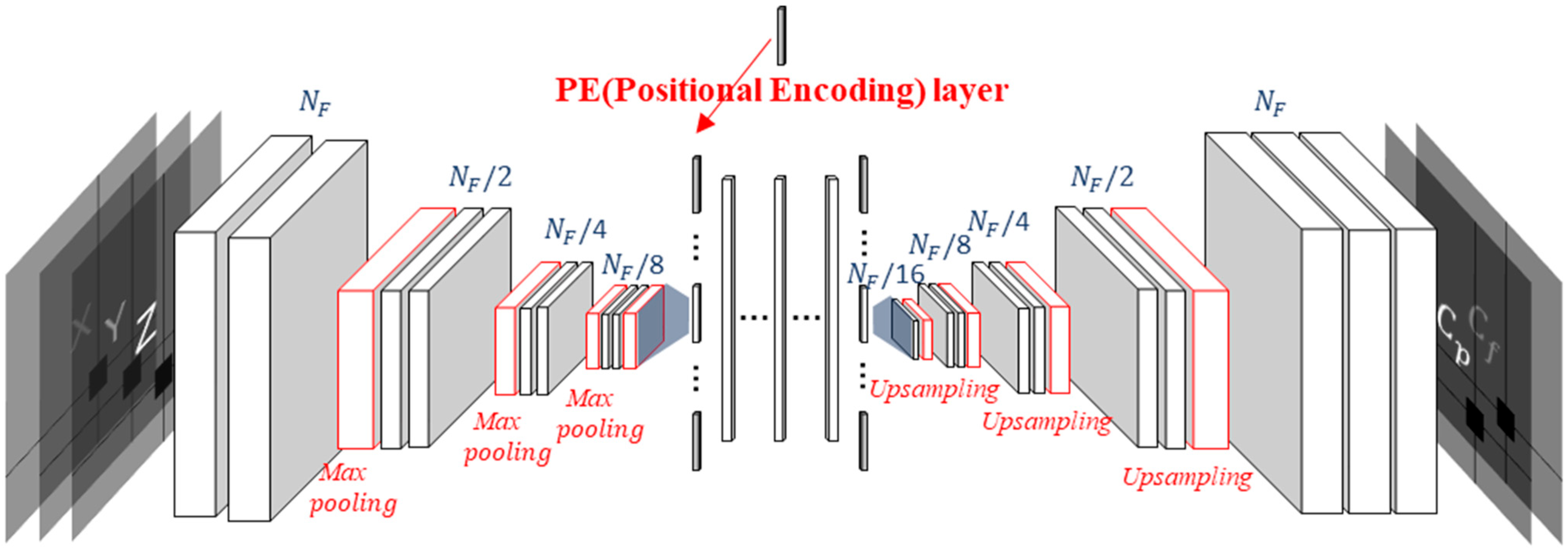
Unlike the classical U-Net formulation, the proposed architecture does not include skip connections between corresponding encoder and decoder layers, as illustrated in Figure 5. Preliminary experiments revealed that direct concatenation of high-resolution encoder features introduced high-frequency geometric noise and amplified seam-adjacent discontinuities on the low-resolution projected grids (128 × 128 and 64 × 64). Removing skip connections produced smoother global feature representations and improved numerical stability without degrading reconstruction accuracy. For this reason, a symmetric encoder–decoder topology without skip connections was adopted.

3.2. Positional Encoding (PE)

3.2.1. Features and Structure of Positional Encoding

To better represent patterns that depend strongly on spatial location—particularly near appendages and on the hull surface—we append a position vector to the feature vector after encoding and immediately before the bottleneck, as illustrated in Figure 6. This approach leverages the property of sinusoidal positional encoding, which allows relative positional changes to be represented through linear transformations (Vaswani et al. [15]). In doing so, the model can reflect changes in pressure and wall shear distributions when identical local geometries appear at different axial or circumferential positions and also mitigates phase-alignment issues arising from left–right and top–bottom symmetries (Su et al. [16]).

In this study, positional information is fused at the bottleneck as a one-dimensional vector: each part’s encoder feature map is flattened and then concatenated with a 2D sinusoidal PE vector before entering the fully connected (FC) layers. The FC stack can learn linear and nonlinear combinations over both absolute and relative positional cues contained in the input, while multi-frequency PE simultaneously captures low- to high-frequency variations—effectively modeling high-gradient regions near appendages and distribution shifts with circumferential and axial position. This choice is motivated by the ease with which sinusoidal PE supports the learning of relative positional regularities (Vaswani et al. [15]) and by empirical observations indicating that multi-frequency encodings improve the fidelity of high-frequency details (Mildenhall et al. [17]).

3.2.2. Formal Definition of Positional Encoding

Let input X be a 3D tensor with height H, width W, and channels C, i.e., $\mathrm{X}\in {\mathrm{R}}^{\mathrm{H}\times \mathrm{W}\times \mathrm{C}}$. For a grid index $\left(\mathrm{i},\mathrm{j}\right)\in \left\{0,1,\cdots ,\mathrm{H}-1\right\}\times \{0,1,\cdots ,\mathrm{W}-1\}$, the normalized coordinates are defined by taking the horizontal axis as u and the vertical axis as $\mathrm{v}:$

$$\mathrm{v}={\displaystyle \frac{\mathrm{i}}{\mathrm{H}-1}}, u = {\displaystyle \frac{j}{W - 1}}\left(\in \left[0,1\right]\right)$$

(1)

Let the total number of PE channels be an even integer d. Because each axis uses sine–cosine pairs (two channels per frequency), we set the per-axis channel count to 2M2M2M and the overall channel count to $4\mathrm{M}=\mathrm{d}$, i.e.,

$$\mathrm{M}={\displaystyle \frac{\mathrm{d}}{4}}, u, v\in [0, 1]$$

(2)

For normalized coordinates $(\mathrm{u},\mathrm{v})$, define a logarithmically spaced frequency set

$${\mathrm{f}}_{\mathrm{k}}=f_{min}{\left({\displaystyle \frac{{\mathrm{f}}_{\mathrm{m}\mathrm{a}\mathrm{x}}}{f_{min}}}\right)}^{{\displaystyle \frac{k}{M-1}}}, u,v\in [0,1]$$

(3)

and the corresponding angular frequencies ${\mathsf{\omega }}_{\mathrm{k}}= 2\pi f_k$. The per-axis sinusoidal encodings are

$${\mathrm{P}}_{\mathrm{x}}\left(u\right)=\left[\sin \left({\mathsf{\omega }}_0\mathrm{u}\right),\cos \left({\mathsf{\omega }}_0\mathrm{u}\right),\cdots ,\sin \left({\mathsf{\omega }}_{\mathrm{M}-1}\mathrm{u}\right),\cos \left({\mathsf{\omega }}_{\mathrm{M}-1}\mathrm{u}\right)\right]ϵ{\mathrm{R}}^{2\mathrm{M}}$$

(4)

$${\mathrm{P}}_{\mathrm{y}}\left(v\right)=\left[\sin \left({\mathsf{\omega }}_{0}v\right),\cos \left({\mathsf{\omega }}_{0}v\right),\cdots ,\sin \left({\mathsf{\omega }}_{\mathrm{M}-1}v\right),\cos \left({\mathsf{\omega }}_{\mathrm{M}-1}v\right)\right]ϵ{\mathrm{R}}^{2\mathrm{M}}$$

(5)

and the 2D positional vector at a point (u, v) (u, v) (u, v) is the channel-wise concatenation

$$\mathrm{P}\left(\mathrm{u},\mathrm{v}\right)=\left[{\mathrm{P}}_{\mathrm{x}}\left(\mathrm{u}\right)‖P_y\left(v\right)\right]\in {\mathrm{R}}^{\mathrm{d}}$$

(6)

Stacking $\mathrm{P}\left(\mathrm{u},\mathrm{v}\right)$ over the spatial grid yields a positional-channel tensor

$$\mathrm{P}=\left\{{\mathrm{P}}_{\mathrm{i},\mathrm{j}}\right\}\in {\mathrm{R}}^{\mathrm{H}\times \mathrm{W}\times \mathrm{d}}$$

(7)

Let $\mathrm{F}\in {\mathrm{R}}^{\mathrm{H}\times \mathrm{W}\times {\mathrm{C}}_{\mathrm{f}}}$ denote the feature map immediately before the bottleneck for a given part. We inject positional channels via channel-wise concatenation,

$$\mathrm{Z}=\left[\mathrm{F}‖P\right]\in {\mathrm{R}}^{\mathrm{H}\times \mathrm{W}\times \left({\mathrm{C}}_{\mathrm{f}}+d\right)}$$

(8)

after which Z is flattened and fed directly to the fully connected (FC) layers.

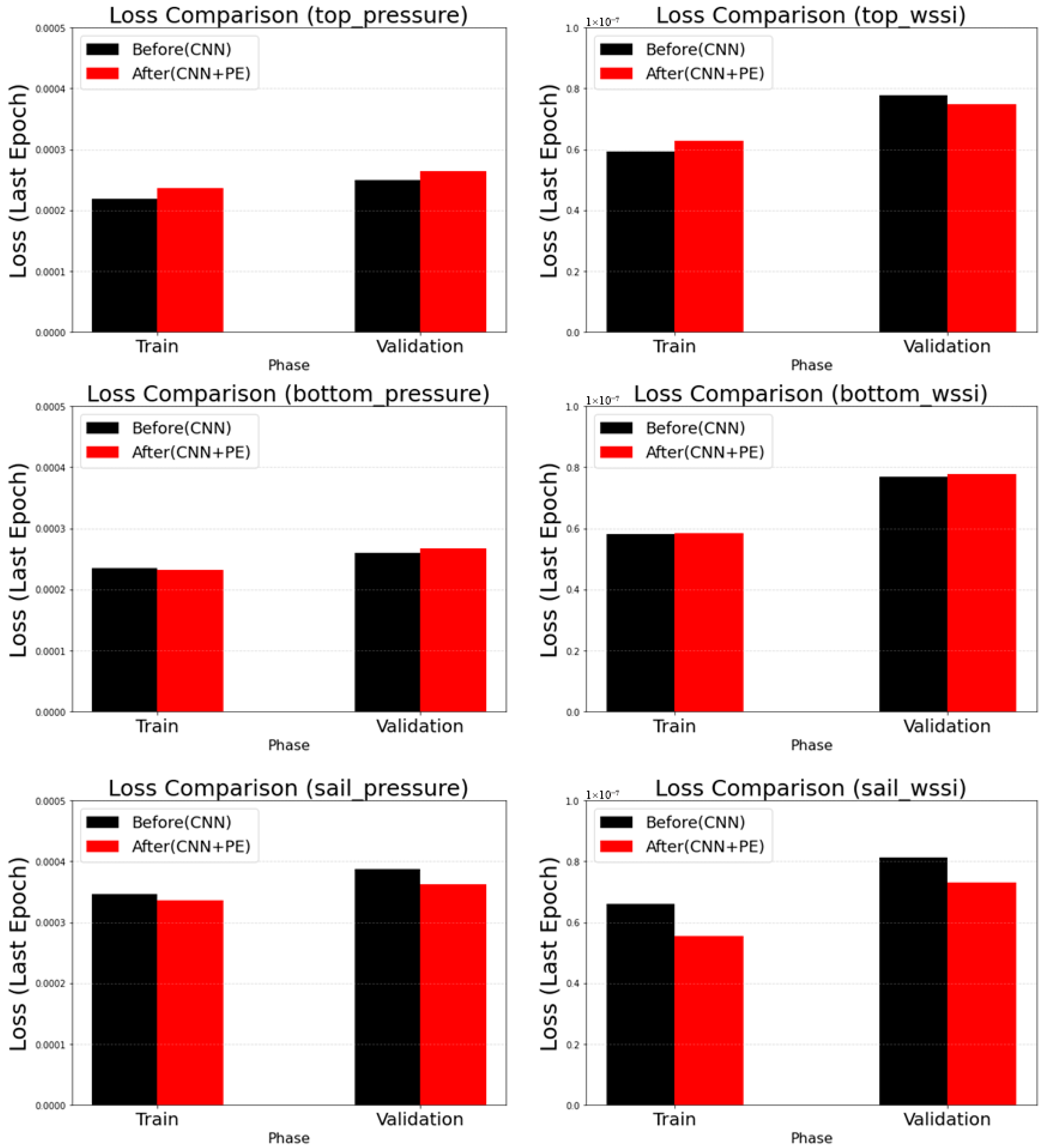
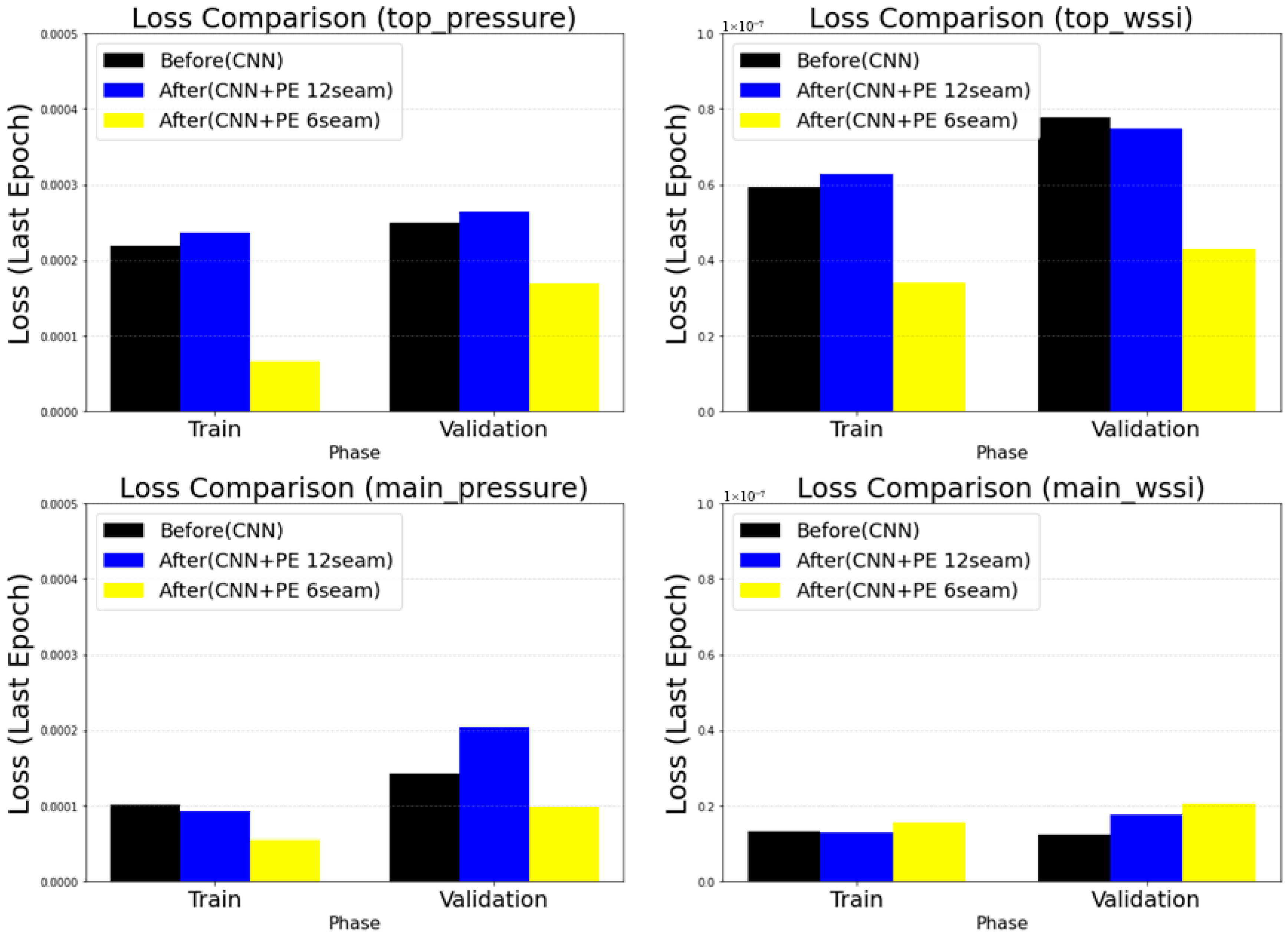
Compared with the baseline U-Net, U-Net+PE exhibits improved performance because the injected PE provides multi-frequency cues—log-spaced from low to high frequencies—that encode both global and local positional information, enabling stable representation of high-gradient regions near the sail and rudders as well as along the axial and circumferential directions. The performance difference between the two settings is reported by the loss values at epoch 500 in Figure 7: while training errors tend to increase slightly for parts other than the sail, the sail exhibits a marked error reduction. Since the sail’s ${\mathrm{C}}_{\mathrm{p}}$ error was the largest, we adopted the U-Net+PE configuration to mitigate it. Section 3.3 introduces additional remedies to further reduce errors observed for the main hull and the four rudders.

In the sinusoidal positional encoding used in this study, the embedding dimension d is not an independent hyperparameter. Since each frequency band generates a sine–cosine pair for both surface coordinates (u, v), each band contributes four channels to the encoding. Following the standard multi-frequency formulation used in Transformers [15] and NeRF-style encodings [16], the total encoding dimension is therefore determined by $\mathrm{d}=4\mathrm{M}$, where M is the number of frequency bands. Accordingly, only M represents a tunable hyperparameter, whereas d is a deterministic consequence of the PE formulation.

3.3. Relocation of the Seam

3.3.1. Motivation

In the initial projected grid, the circumferential coordinate starts at 12 o’clock and is ordered clockwise. Consequently, the high-gradient region near the sail around 12 o’clock coincides with the seam, causing the pressure and shear distributions to be split at the grid boundary. This leads to boundary discontinuity artifacts during interpolation and training, and during integration, this separates information on the two sides of the boundary, resulting in local information loss. To mitigate these effects, the seam is relocated to 6 o’clock, which is comparatively less critical than the 12 o’clock region. A schematic view of the main hull highlighting the locations of the 12 o’clock and 6 o’clock seams is shown in Figure 8.

3.3.2. Relocation Method

The relocation is a coordinate transformation that shifts the circumferential reference from 12 o’clock to 6 o’clock; the geometry, area vectors, and normals remain unchanged. In the continuous coordinates (u, v), the circumferential coordinate is shifted as

$$\tilde{v}=\mathrm{m}\mathrm{o}\mathrm{d}\left(\mathrm{v}+{\displaystyle \frac{1}{2}},1\right)$$

(9)

while on a discrete grid, the same rule is applied by cyclically shifting the column indices (implemented for the main hull):

$$\tilde{J}=\mathrm{m}\mathrm{o}\mathrm{d}\left(\mathrm{j}+{\displaystyle \frac{\mathrm{W}}{2}},\mathrm{W}\right)$$

(10)

For completeness, the modulo operation is defined for integers a and $\mathrm{n} (\mathrm{n}>0)$ as

$$\mathrm{a} \mathrm{m}\mathrm{o}\mathrm{d} \mathrm{n}=\mathrm{r}, \mathrm{a}=\mathrm{q}\mathrm{n}+\mathrm{r}, 0\le \mathrm{r}<\mathrm{n}, \mathrm{q}\in \mathrm{Z}$$

(11)

Because the grid is normalized, the above shift corresponds to a half-turn rotation.

To isolate the individual contribution of seam relocation, an additional baseline model was trained using 12 o’clock and 6 o’clock seams without positional encoding (PE). Figure 9 compares the training and validation losses of the two configurations. The results show that U-Net alone does not benefit from seam relocation, and in fact, the 6 o’clock seam configuration exhibits slightly higher loss across most epochs. This indicates that seam relocation by itself does not improve prediction accuracy and that its effectiveness is closely tied to the presence of PE, which provides global positional cues that help the model correctly interpret the discontinuity region. Consequently, the performance gain demonstrated in the main model originates from the combined effect of PE and seam relocation, rather than from seam relocation alone.

3.3.3. Quantitative Evaluation of the Seam

To quantify the effect of seam relocation on boundary discontinuities, we evaluated the interpolation error across the seam line for both configurations. Specifically, we computed the mean absolute difference of ${\mathrm{C}}_{\mathrm{p}}$ between pairs of cells located on either side of the seam. For the 12 o’clock seam, the mean ${\mathrm{C}}_{\mathrm{p}}$ seam error is $8.84\times {10}^{-3}$, whereas for the 6 o’clock seam, it decreased to $1.3\times {10}^{-3}$, corresponding to an 85.3% reduction. This confirms that relocating the projection seam away from the high-gradient region near the sail substantially alleviates the artificial discontinuity in the pressure field.

For the wall shear stress coefficient ${\mathrm{C}}_{\mathrm{f}}$, the mean seam error for the 6 o’clock configuration was $5.94\times {10}^{-5}$, which is more than an order of magnitude smaller than the corresponding ${\mathrm{C}}_{\mathrm{p}}$ seam error. This indicates that, after seam relocation, the residual discontinuity in the shear field is negligible compared with typical field magnitudes.

3.4. Machine Learning Training

3.4.1. Inputs and Normalization

The inputs comprise 2D grid images for six parts: the main hull, the sail, and the top/bottom/port/starboard rudders. Through preprocessing, the main hull is mapped to a matrix of size 128 × 128 × 3, while the remaining parts use 64 × 64 × 3. All data were aligned with the seam placed at 6 o’clock (see Section 3.3). Target fields are nondimensionalized as the pressure coefficient $\left({\mathrm{C}}_{\mathrm{p}}\right)$ and the skin friction coefficient $\left({\mathrm{C}}_{\mathrm{f}}\right)$.

Because the magnitudes of the two target fields differ by approximately three orders—${\mathrm{C}}_{\mathrm{p}}= O\left(1\right)$ vs. ${\mathrm{C}}_{\mathrm{f}}=O\left({10}^{-3}\right)$—a direct multi-output regression would cause the loss to be dominated by the pressure coefficient term. To balance the contributions of the two learning targets, the loss associated with ${\mathrm{C}}_{\mathrm{f}}$ was scaled by a factor of $\mathsf{\lambda }={10}^3$, ensuring that both gradients remain of comparable magnitude during optimization. This weighting strategy is consistent with common practices in multi-scale regression and prevents the network from converging toward a solution that fits ${\mathrm{C}}_{\mathrm{p}}$ accurately while undertraining ${\mathrm{C}}_{\mathrm{f}}$. Preliminary checks confirmed that $\mathsf{\lambda }={10}^3$ provides stable convergence and avoids gradient collapse, and a broader sensitivity study was therefore deemed unnecessary for the scope of the present work.

3.4.2. Fully Connected Network and Part-Wise Decoders

For each part, the feature map just before the bottleneck (after concatenation with positional encoding) is flattened; the flattened vectors from all parts are concatenated and fed to a three-layer fully connected (FC) network h. The FC output is then split into part-specific segments, reshaped to match the original feature map sizes, and supplied to the corresponding part-wise decoders. Each decoder restores spatial resolution by repeating a convolution → upsampling → convolution sequence. We denote the PE-augmented feature map for part p by ${\mathrm{F}}_p^{\mathrm{P}\mathrm{E}}$.

3.4.3. Outputs and Loss

At the end of each part-wise decoder, two parallel 1 × 1 convolution heads are used to predict two scalar fields simultaneously: ${\mathrm{C}}_{\mathrm{p}}$ and ${\mathrm{C}}_{\mathrm{f}}$. With six parts and two fields per part, the network produces twelve outputs in total.

Let the prediction–ground truth pairs be $({\mathrm{C}}_p^{\mathrm{p}\mathrm{r}\mathrm{e}\mathrm{d}},C_p^{ture})$ and $({\mathrm{C}}_f^{\mathrm{p}\mathrm{r}\mathrm{e}\mathrm{d}},C_f^{true})$ for each part p. The field loss over the part set P is the sum of mean squared errors (MSEs) for ${\mathrm{C}}_{\mathrm{p}}$ and ${\mathrm{C}}_{\mathrm{f}}$, with an additional weight λ on the ${\mathrm{C}}_{\mathrm{f}}$ term to account for scale differences and to prevent training from focusing on a single field.

$${\mathrm{L}}_{\mathrm{f}\mathrm{i}\mathrm{e}\mathrm{l}\mathrm{d}}={\sum }_{p\in P}[MSE\left(C_p^{pred},C_p^{true}\right)+\lambda MSE(C_f^{pred},C_f^{true}\left)\right]$$

(12)

In our experiments, we set $\mathsf{\lambda }={10}^3$.

3.5. Experimental Design

3.5.1. Data Composition

Data splits follow a fixed rule: IDs 91–500 are used for training, and IDs 1–90 for validation. Cases that diverged during STAR-CCM+ computations were excluded prior to training and were not used for either training or validation.

To prevent geometric correlation leakage between the training and validation sets, a non-random, index-based split was adopted. Because the SUBOFF variants are generated via systematic FFD perturbations, randomly shuffling the dataset would distribute geometrically similar shapes—often differing by only small master point displacements—across both sets, artificially improving the apparent generalization performance. By assigning IDs 1–90 exclusively to validation, the model is evaluated on variants that are geometrically distinct from those seen during training, thereby providing a more conservative and physically meaningful assessment of prediction accuracy.

While k-fold cross-validation could, in principle, increase statistical robustness, each fold would require the full training of a multi-output U-Net over high-resolution surface fields, resulting in computational demands far exceeding typical surrogate modeling practices for CFD-based submarine datasets. Consistent with prior learning-based hydrodynamic studies on SUBOFF and ship hull flows, which commonly rely on fixed training–test splits, we employed a single, geometry-independent validation subset that nonetheless spans the full range of deformation modes (M1–M9). This strategy provides stable and conservative evaluation while maintaining computational feasibility.

3.5.2. Baselines for Comparison

To assess the effects of positional encoding (PE) and preprocessing, we constructed four alternative models and compared their training errors. All baseline models use the same data split described in Section 3.5.1 (training: IDs 91–500; validation: IDs 1–90) and were trained for 500 epochs with all other hyperparameters kept constant. The baseline configurations are summarized in

Table 4. Baseline models.

Model ID	Description
MO0	Pure CNN predicting ${\mathrm{C}}_{\mathrm{p}}$ and ${\mathrm{C}}_{\mathrm{f}}$
MO1	Positional encoding (PE) concatenated to the feature maps after the encoder
MO2	Same as MO1, but with the seam relocated to 6 o’clock during preprocessing

.

3.5.3. Training Setup and Model Selection

Optimization was performed using the Adam optimizer with an initial learning rate of $1\times {10}^{-4}$. Each model was trained for 500 epochs with a mini-batch size of 10; early stopping was not applied. All twelve heads (six parts × two fields) were trained jointly, and optimization followed Keras’s multi-output objective defined as the sum of MSE losses. Model selection was based on validation loss and training loss at epoch 500.

The comparative results are summarized below.

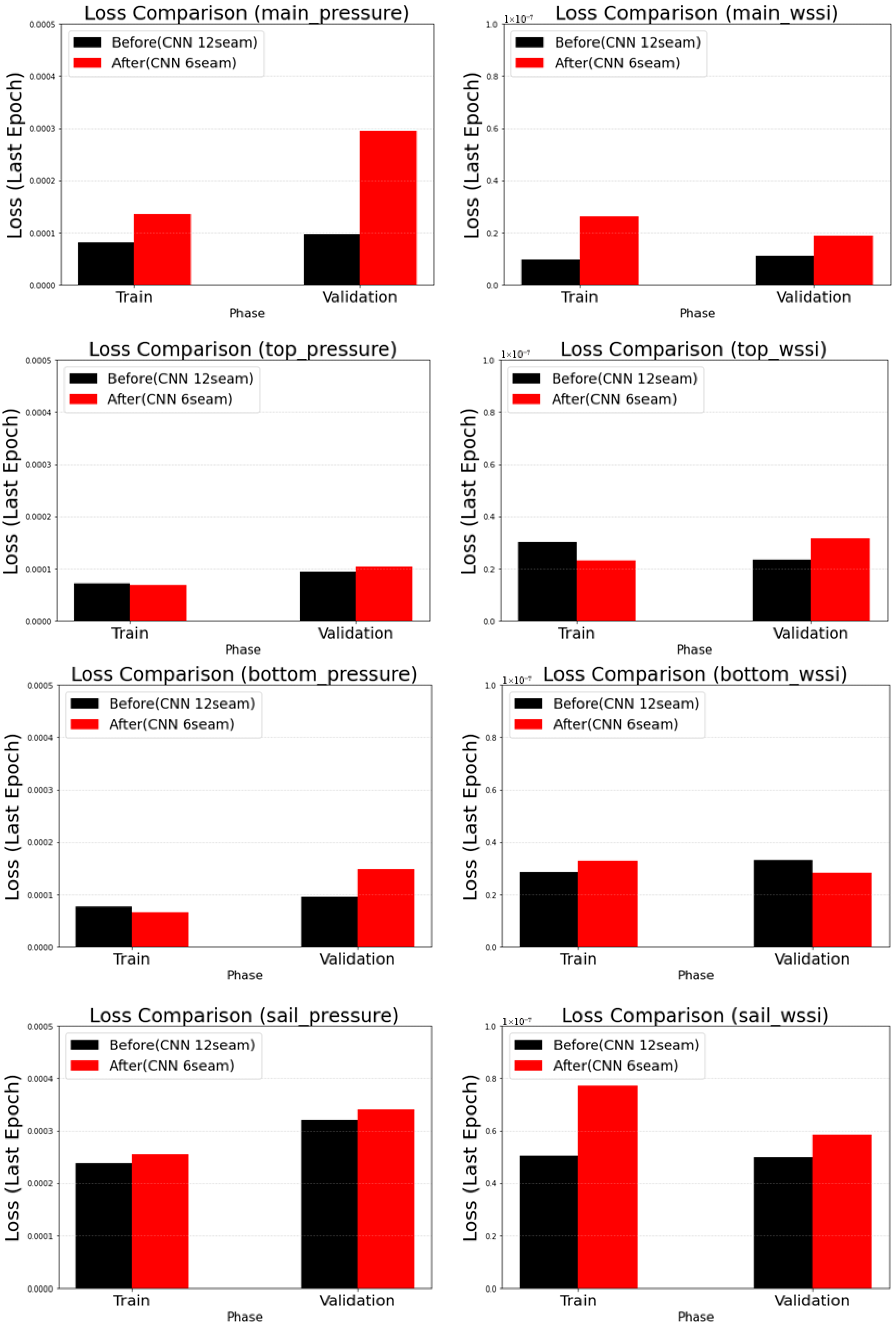
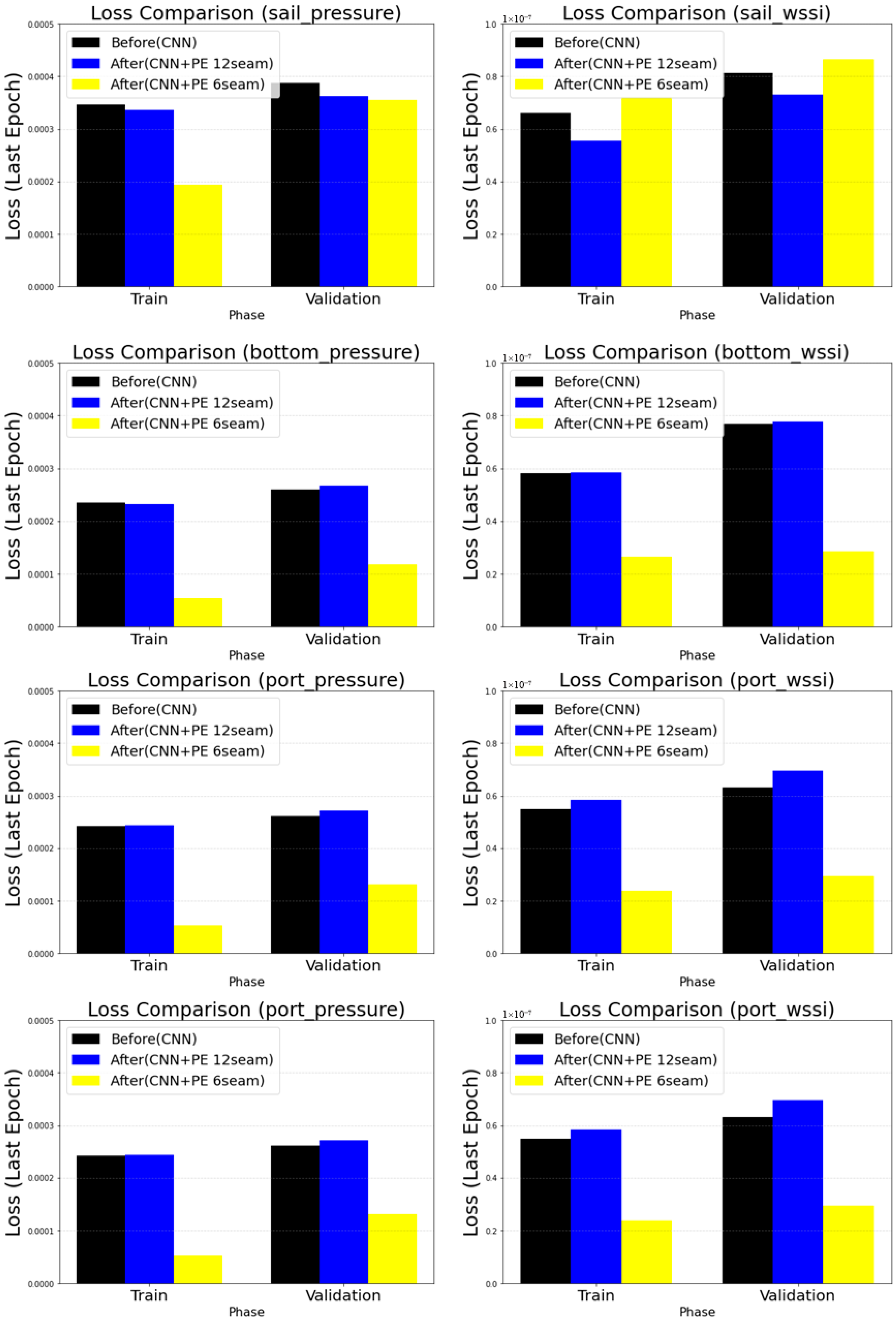
Figure 7 compares a CNN with a 12 o’clock seam against a CNN + PE model (also with a 12 o’clock seam). Figure 10 extends the comparison to include a CNN + PE model with the seam relocated to 6 o’clock. As discussed in Section 3.2.2, the CNN + PE model (12 o’clock seam) reduced loss for the sail, whereas losses increased for the main part, as well as the other parts. When PE was combined with the 6 o’clock seam, losses decreased relative to the pure-CNN baseline for all targets except (i) main friction and (ii) sail friction, whose validation losses remained higher. Overall, these results indicate that injecting PE and relocating the seam generally improve predictive performance across most parts. Beyond convolutional features and positional channels, operator learning frameworks such as the Fourier Neural Operator provide a mesh-independent mapping between function spaces and may further complement the present approach (Li et al. [17]).

Although Figure 7 and Figure 11 report only the final epoch losses for brevity and readability, the full training and validation curves were also examined to ensure convergence and to monitor potential overfitting. All models exhibited monotonic or weakly oscillatory loss reduction without divergence, and no overfitting behavior was observed within 500 epochs. Accordingly, the final epoch values were adopted as the basis for comparison.

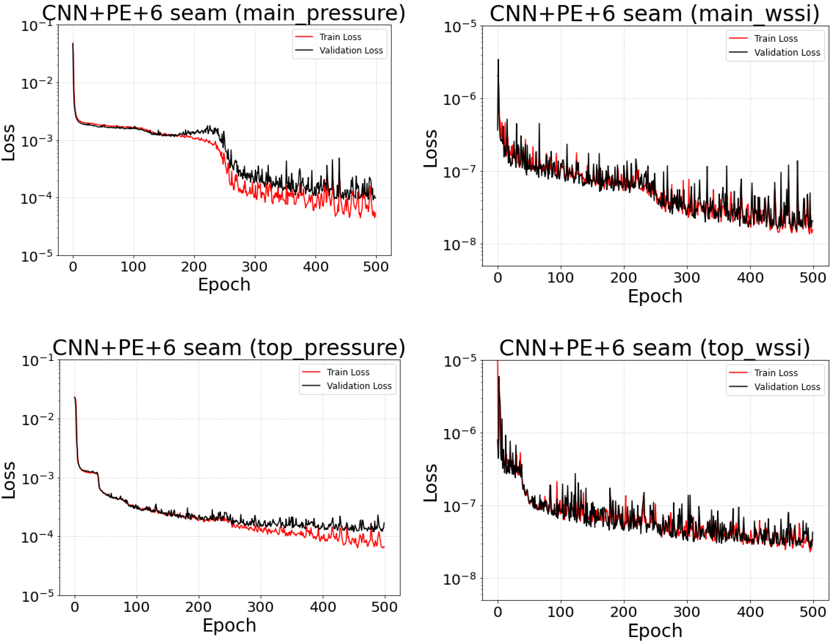
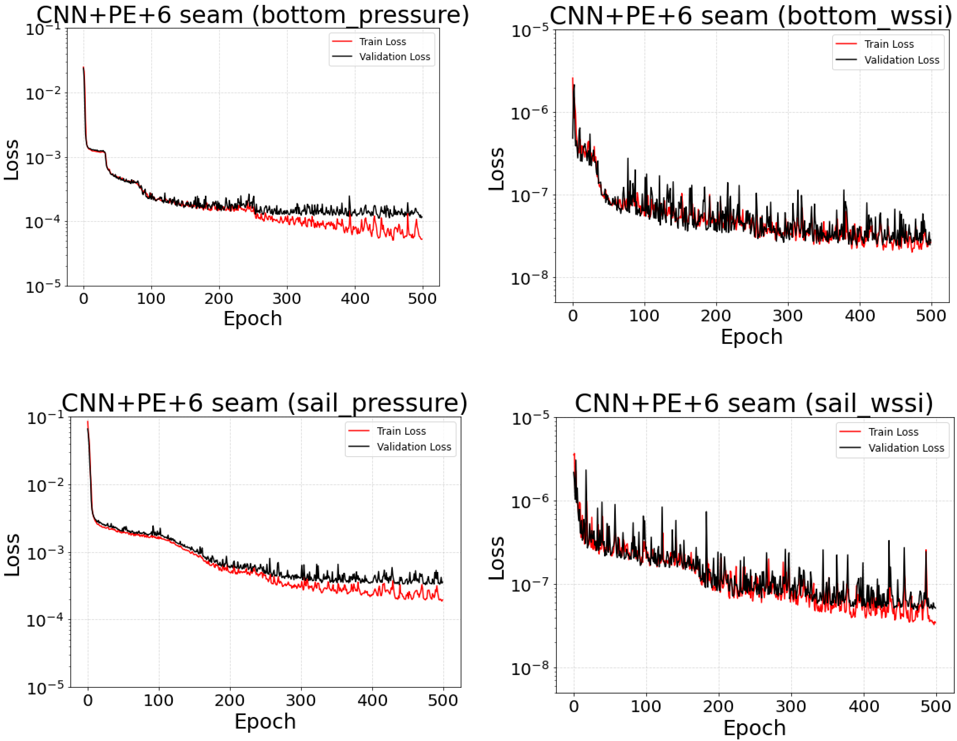
To further examine convergence characteristics and training stability, Figure 10 presents the full training and validation loss curves for the final model (U-Net + PE with the 6 o’clock seam). Both losses exhibit a clear downward trend over 500 epochs, with the training and validation curves remaining closely aligned throughout. Although the validation loss shows moderate oscillations—typical for high-resolution multi-output regression—the overall convergence behavior is stable, and no overfitting is observed. While Figure 7 and Figure 11 report only the final epoch losses for visual clarity, all tested models demonstrated similarly consistent convergence patterns.

In this study, the Adam optimizer was used with a fixed learning rate of 1 × 10⁻⁴, and no learning rate scheduling or decay policy was applied. Preliminary tests confirmed that this constant learning rate ensured stable and monotonic convergence for all baseline configurations, and maintaining identical optimization settings facilitated a fair comparison between the proposed and baseline models. A mini-batch size of 10 was selected as a compromise between convergence stability and hardware constraints. Because each training sample includes high-resolution matrices for six geometric parts, increasing the batch size led to GPU memory overflow on the available hardware (RTX 3080, 10 GB). A batch size of 10 provided stable training dynamics and efficient memory usage, and no degradation in convergence behavior was observed with this setting.

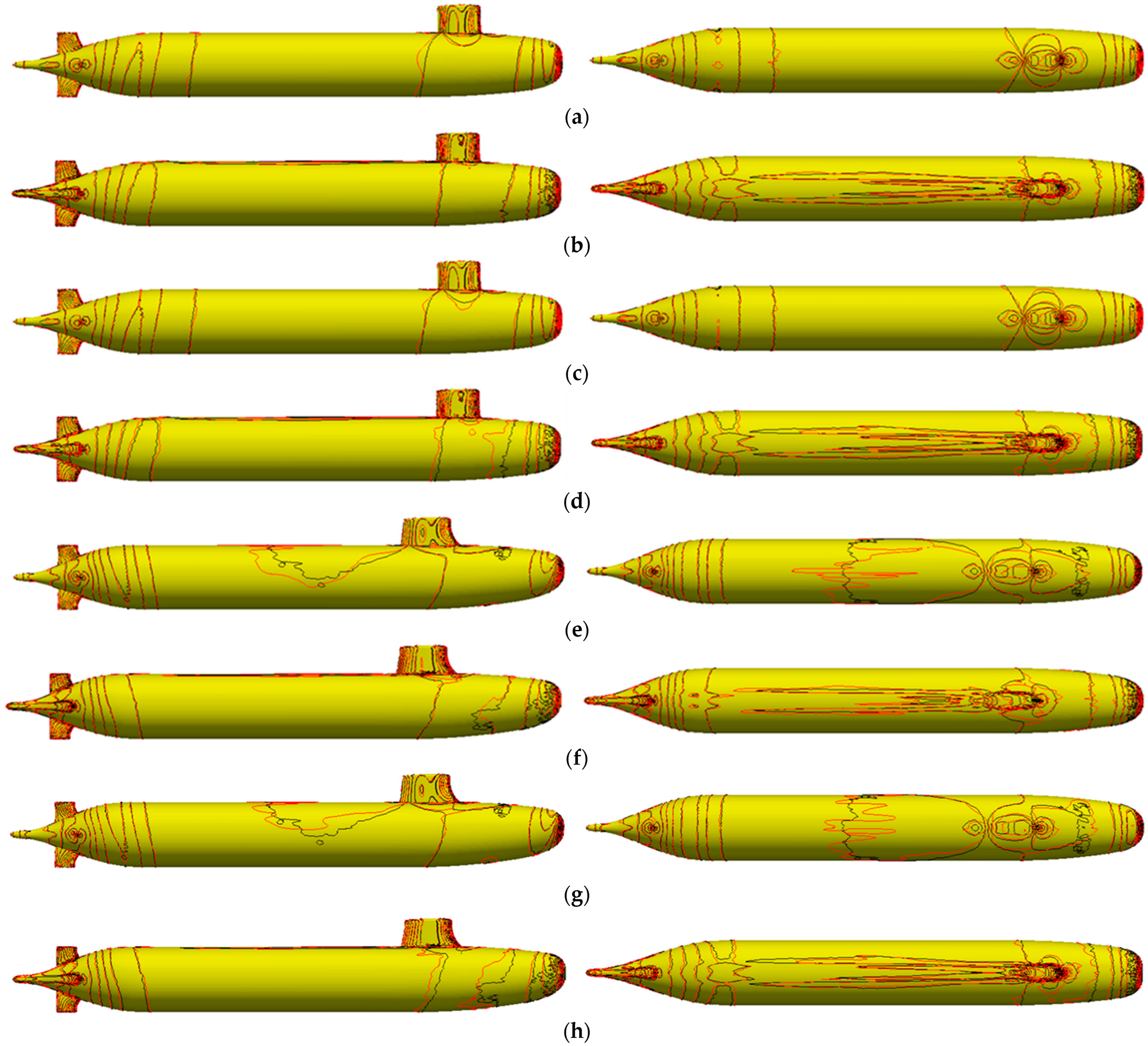
Figure 12 compares the predicted surface pressure and wall shear stress distributions for two representative DARPA SUBOFF variants, Cases 5 and 120.

For each case, panels (a, c, e, g) and (b, d, f, h) show the pressure coefficient (${\mathrm{C}}_{\mathrm{p}}$) and wall shear stress coefficient (${\mathrm{C}}_{\mathrm{f}}$) contours, respectively. The upper four panels (a–d) correspond to Case 5, and the lower four (e–h) correspond to Case 120; within each case, the first two panels display the CNN-only results, and the latter two present the CNN + PE model with the seam relocated to 6 o’clock. In both variants, the CNN-only model shows local discontinuities and asymmetric patterns near the sail–hull junction and the stern region, whereas the CNN + PE model provides smoother and more circumferentially continuous contour distributions. In Case 120, which involves larger deformation around the afterbody, slight improvements are observed in the pressure recovery region and the uniformity of wall shear distributions, indicating that the CNN + PE model produces somewhat more stable flow-field predictions without introducing significant artifacts. These results suggest that positional encoding combined with seam relocation contributes to modest yet consistent improvements in spatial continuity and overall predictive fidelity across different hull configurations.

3.5.4. Evaluation of Prediction Metrics

We evaluate the streamwise (drag direction) integrated quantities using the mean absolute percentage error (MAPE). For an indicator $\mathrm{s}\in \{{\mathrm{C}}_{\mathrm{p}}, {\mathrm{C}}_{\mathrm{f}}, {\mathrm{C}}_T\}$ and N cases, MAPE is defined as

$${\mathrm{M}\mathrm{A}\mathrm{P}\mathrm{E}}_{int}^{\mathrm{s}}\left(\%\right)={\displaystyle \frac{100}{N}}{\sum }_{k=1}^N{\displaystyle \frac{\left|D_{x,k}^s\left(pred\right)-D_{x,k}^s\left(true\right)\right|}{\left|D_{x,k}^s\left(true\right)\right|}}$$

(13)

Here, ${\mathrm{D}}_x^{\mathrm{s}}$ denotes the area-integrated x-component (drag direction) of the field s on the surface. We also define the total coefficient ${\mathrm{C}}_{\mathrm{T}}=C_p+C_f$ and its integrated drag as

$${\mathrm{D}}_x^{{\mathrm{C}}_{\mathrm{T}}}=D_x^{C_p}+D_x^{C_f}$$

(14)

3.5.5. Visualization and Diagnostic Analysis

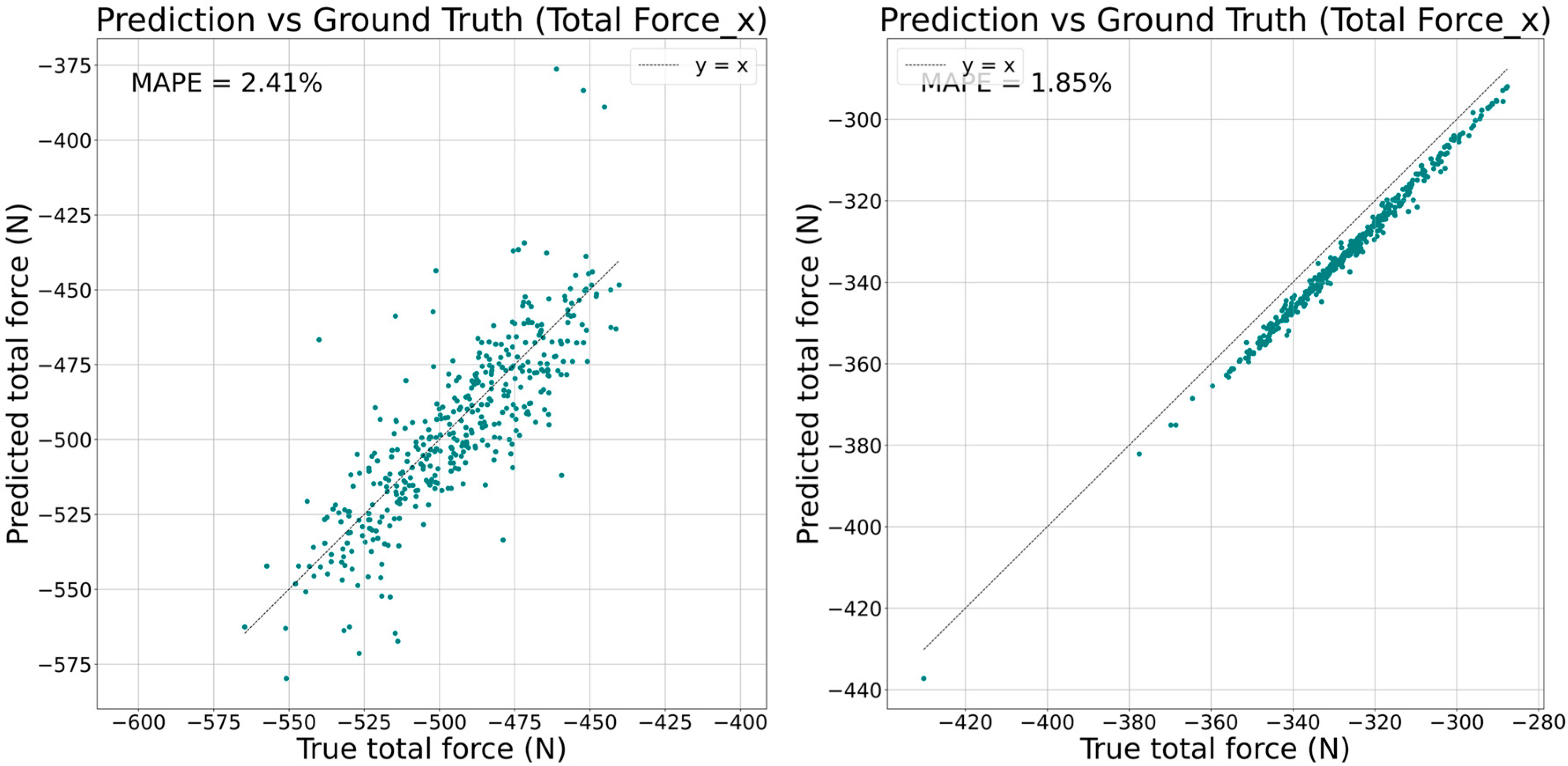
To assess overall agreement, we compare the total streamwise integral using scatter plots: the horizontal and vertical axes show the reference ${\mathrm{D}}_x^{{\mathrm{C}}_{\mathrm{T}}}\left(true\right)$ (unit: N) and prediction ${\mathrm{D}}_x^{{\mathrm{C}}_{\mathrm{T}}} \left(pred\right)$, respectively. The ideal agreement line $\mathrm{y}=\mathrm{x}$ is plotted to visualize bias and dispersion. For consistency, both axes use the same units (N) and common ranges, with an equal aspect ratio. Each panel is annotated with the chapter’s primary metric, ${\mathrm{M}\mathrm{A}\mathrm{P}\mathrm{E}}_{int}^{{\mathrm{C}}_{\mathrm{T}}} (\%)$, so that the quantitative indicator and the scatter visualization convey bias and variance together.

3.5.6. Spatial Error Map

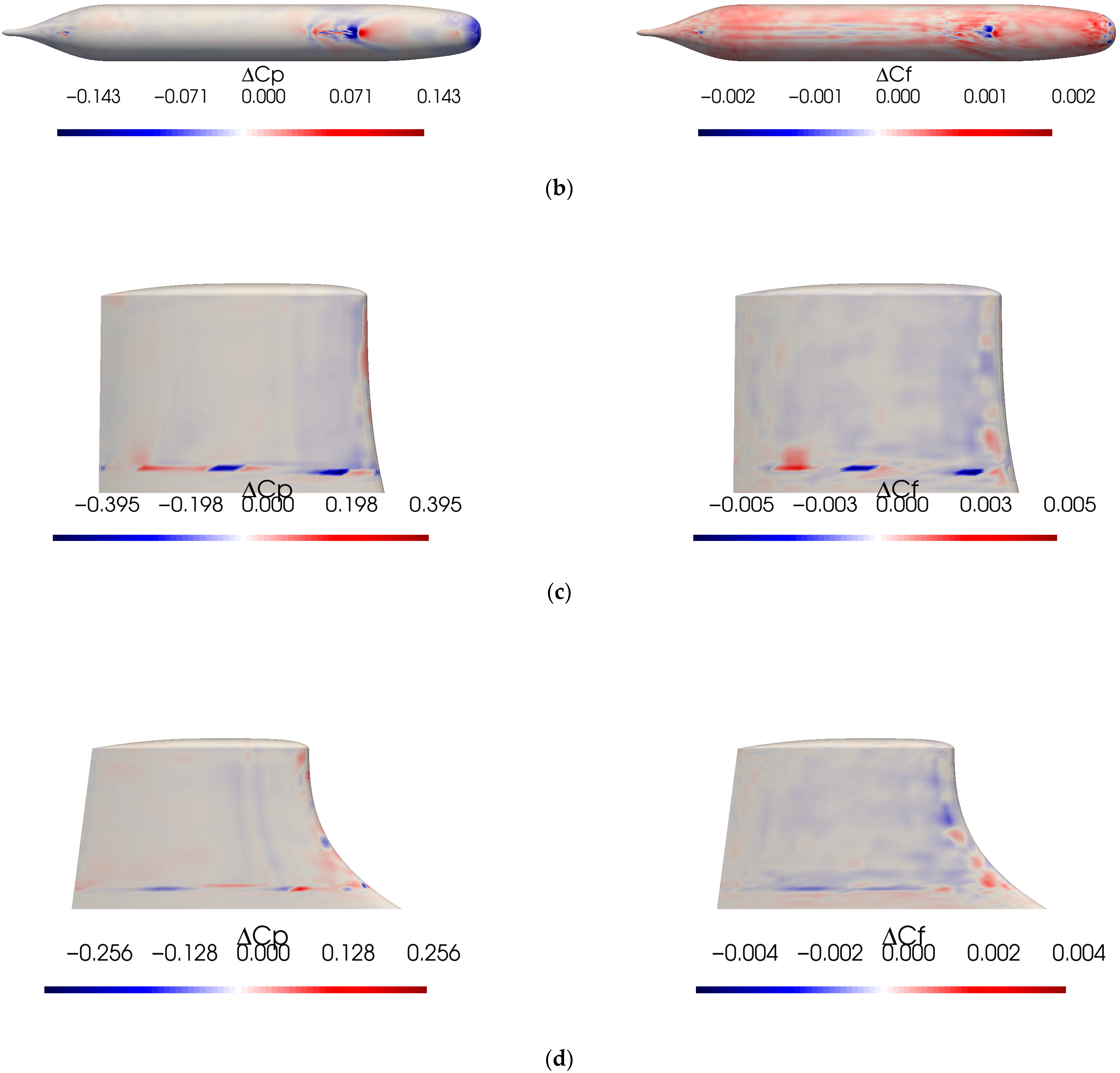
Figure 13 presents spatial error maps of Δ${\mathrm{C}}_{\mathrm{p}}$ and Δ${\mathrm{C}}_{\mathrm{f}}$ to assess the local prediction accuracy of the proposed network beyond global metrics such as MSE and drag-integrated MAPE. Field-level prediction problems require diagnostics capable of revealing model behavior in high-gradient regions—such as the aft-body pressure recovery zone, the sail–hull junction, and areas of sharp curvature changes—where small geometric perturbations can induce large variations in the pressure and shear fields. The spatial maps provided here address this requirement by visualizing local discrepancies across representative variants.

Subfigure (a) shows the error distributions on the main body for Case 5. The errors remain small and relatively uniform along the length of the hull, with only mild localized deviations near the aft-body region where curvature begins to increase. This indicates that for geometries with limited perturbation, the model reproduces the surface flow fields with high reliability. In contrast, Subfigure (b) corresponds to Case 120 and exhibits noticeably larger and more concentrated Δ${\mathrm{C}}_{\mathrm{p}}$ and Δ${\mathrm{C}}_{\mathrm{f}}$ errors, particularly within the aft-body pressure recovery region, where alternating positive and negative gradients form. These discrepancies reflect the increased prediction difficulty in flows dominated by strong adverse pressure gradients and three-dimensional shear-layer interactions.

Subfigures (c,d) show the corresponding error maps on the sail. For Case 5, the errors are mainly distributed around the sail–hull junction and the lower lateral surfaces, but their magnitude remains modest. The model captures the sail flow reasonably well when geometric variation is small. For Case 120, however, the error magnitude increases significantly near the sail root and the trailing-edge region, with localized high-frequency patterns evident in both Δ${\mathrm{C}}_{\mathrm{p}}$ and Δ${\mathrm{C}}_{\mathrm{f}}$. This behavior is consistent with the physical sensitivity of the sail boundary layer to geometric perturbation, as small changes in curvature can modify separation and reattachment characteristics, making the flow more challenging to predict.

Overall, the spatial error maps provide crucial insight into how the model behaves across different geometric conditions and flow environments. They reveal that while the proposed U-Net+PE architecture performs robustly for moderate geometries, localized challenges remain in high-gradient regions where the underlying flow physics exhibit strong nonlinear sensitivity. Such diagnostics complement global accuracy metrics and enhance the physical interpretability and reliability assessment of the model.

In addition, the results indicate that the wall shear stress coefficient ${\mathrm{C}}_{\mathrm{f}}$ is substantially more difficult to predict than the pressure coefficient ${\mathrm{C}}_{\mathrm{p}}$, especially around the sail and rudders. Physically, ${\mathrm{C}}_{\mathrm{f}}$ depends on the gradient of the tangential velocity within the near-wall viscous sublayer, so even small discrepancies in the reconstructed velocity field or boundary-layer state are amplified into relatively large errors in ${\mathrm{C}}_{\mathrm{f}}$. In contrast, ${\mathrm{C}}_{\mathrm{p}}$ is governed by the pressure field, which varies more smoothly along the surface and is less sensitive to local geometric details. The sail and rudders exhibit strong curvature, junction flows, and locally high adverse pressure gradients, so the near-wall shear distribution is highly sensitive to subtle shape modifications and to the exact location of separation and reattachment. Consequently, the proposed model still shows localized error hot spots in these appendage regions, despite its overall improvement in ${\mathrm{C}}_{\mathrm{f}}$ prediction accuracy.

Beyond identifying local prediction discrepancies, the spatial maps also provide an effective means with which to evaluate the continuity of the reconstructed fields. The spatial error maps for Δ${\mathrm{C}}_{\mathrm{p}}$ and Δ${\mathrm{C}}_{\mathrm{f}}$ act as quantitative indicators of spatial continuity. Because each map directly reflects the pointwise error relative to the CFD reference fields, high-frequency variations or localized peaks identify areas where continuity is degraded, particularly near the projection seam and at appendage–hull junctions. When comparing the baseline and proposed models under the same color scale, the visibly smoother error patterns and the reduction in localized spikes indicate an improvement in spatial continuity.

3.5.7. Analysis of the Influence of Positional Encoding

The incorporation of positional encoding (PE) provides explicit spatial information that is otherwise lost during 3D-to-2D projection, enabling the network to better distinguish flow patterns associated with curvature, orientation, and local coordinate variations. However, the magnitude of improvement is not uniform across all components. The main hull, with its relatively smooth curvature and gradual pressure variations, benefits modestly because the baseline CNN already captures most large-scale flow features. In contrast, the sail and rudders exhibit sharper curvature changes, junction flows, and localized high-gradient regions, where small geometric perturbations generate disproportionately large variations in ${\mathrm{C}}_{\mathrm{p}}$ and ${\mathrm{C}}_{\mathrm{f}}$. In these areas, PE helps the model preserve spatial coherence and reduces misalignment between geometry-induced features and their projected coordinates, leading to more noticeable accuracy gains.

Nonetheless, improvements in ${\mathrm{C}}_{\mathrm{f}}$ remain less consistent than those in ${\mathrm{C}}_{\mathrm{p}}$. This is attributed to the inherently higher sensitivity of wall shear stress to near-wall resolution, curvature-induced strain rates, and mapping under-resolution. In regions where the projected grid fails to represent thin shear layers or separation/reattachment lines, PE alone cannot fully compensate for the loss of fine-scale information. This explains why PE enhances overall predictive fidelity but yields uneven improvements across hull components.

4. Summary and Key Findings

Figure 14 visually illustrates the performance improvement achieved by the proposed approach, comparing the predicted distributions of a CNN-only model (left) and those of a CNN + PE model with the seam relocated to 6 o’clock (right). For the DARPA SUBOFF variant dataset, we established a consistent pipeline comprising part segmentation, nondimensionalization, matrix mapping, learning, surface restoration, and area integration and incorporated positional encoding (PE) into the U-Net after the encoder through feature map concatenation. In addition, we relocated the projection grid seam from 12 o’clock to 6 o’clock, alleviating boundary discontinuities in high-gradient regions near the sail and rudders. As a result, the proposed model’s agreement in total resistance predictions improved, and its MAPE was significantly reduced, as summarized in

Table 5. MAPE comparison across training settings.

	CNN	CNN + PE (Seam at 12 O’clock)	CNN + PE (Seam at 6 O’clock)
MAPE (%)	2.41	3.61	1.85

.

4.1. Comparison with State-of-the-Art Models

Recent learning-based studies on submarine and ship hull hydrodynamics report error levels that provide a meaningful benchmark for evaluating the present model. PINN-based SUBOFF resistance prediction frameworks typically achieve global error levels between 3 and 8%, depending on the flow regime and boundary condition complexity (Wu et al. [4]; Chu et al. [5]). Spatio-temporal graph neural networks for SUBOFF wake field prediction similarly report errors of comparable magnitude (Guo et al. [6]). In the context of surface field reconstruction, U-Net-based approaches for ship hulls generally exhibit pressure distribution errors around 2–4% (Kim et al. [7]).

In contrast, the proposed PE-enhanced U-Net achieves a significantly lower MAPE of 1.85% for total drag while simultaneously predicting full-field pressure and wall shear stress distributions across multiple appendages. This performance indicates that the model matches or exceeds the accuracy of state-of-the-art methods, even though it addresses a more geometrically complex prediction task. These results demonstrate the competitive advantage of combining part-wise U-Net encoding, positional encoding, and seam relocation for high-fidelity hydrodynamic field prediction.

4.2. Limitations of $C_f$ Prediction

From a numerical perspective, predicting ${\mathrm{C}}_{\mathrm{f}}$ is also more challenging than predicting ${\mathrm{C}}_{\mathrm{p}}$ because the training data inherit the sensitivities of the underlying RANS solver. In our simulations, ${\mathrm{C}}_{\mathrm{f}}$ is computed from the near-wall velocity gradient and turbulence quantities, which are strongly affected by grid clustering, wall-normal resolution, and the choice of turbulence model. As a result, the ${\mathrm{C}}_{\mathrm{f}}$ field can contain larger case-to-case variability and local noise than the corresponding ${\mathrm{C}}_{\mathrm{p}}$ field, particularly in the vicinity of the sail–hull and rudder–hull junctions. In addition, the mapping procedure tends to under-resolve thin high-shear regions around leading and trailing edges, as well as narrow streaks of elevated ${\mathrm{C}}_{\mathrm{f}}$ along separation and reattachment lines. These features occupy only a few cells on the projected grids, so their contribution can be smeared out or diluted when the three-dimensional surface is transformed into two-dimensional matrices. The CNN-based model is therefore trained on data where the extreme peaks of ${\mathrm{C}}_{\mathrm{f}}$ are under-represented both spatially and statistically, while the vast majority of surface points exhibit relatively low ${\mathrm{C}}_{\mathrm{f}}$ levels. This imbalance encourages the network to focus on minimizing the global error in low-shear regions, at the cost of underpredicting local maxima around the sail and rudders. This explains why the proposed model still struggles in certain appendage regions, despite achieving a significant reduction in the overall ${\mathrm{C}}_{\mathrm{f}}$ MAPE.

In light of these factors, the remaining discrepancies in ${\mathrm{C}}_{\mathrm{f}}$ prediction should be interpreted as a numerical and geometric limitation of the training data rather than a deficiency of the network architecture itself. Regions characterized by sharp curvature, strong crossflow, or three-dimensional separation inherently amplify the sensitivity of wall shear stress to local grid spacing and turbulence model behavior. Consequently, even the CFD reference solutions contain small-scale irregularities in these areas, which the learning model cannot fully reconstruct when projected onto fixed-resolution grids. These structural constraints highlight the need for future extensions that incorporate higher-resolution near-wall sampling and unsteady flow information, particularly around the appendage–hull junctions where separation and reattachment dominate the local shear distribution.

4.3. Correlation Between $C_p$ and $C_f$ Errors and Their Impact on Total Resistance

Although pressure coefficient (${\mathrm{C}}_{\mathrm{p}}$) and wall shear stress coefficient (${\mathrm{C}}_{\mathrm{f}}$) fields contribute differently to the total resistance, their prediction errors are not independent. In the present dataset, ${\mathrm{C}}_{\mathrm{p}}$ dominates the pressure drag component and exhibits relatively smooth spatial variation, whereas ${\mathrm{C}}_{\mathrm{f}}$ governs the viscous component and is highly sensitive to local curvature, separation, and near-wall resolution. As described in Section 4.2, ${\mathrm{C}}_{\mathrm{f}}$ errors tend to be localized around appendage junctions and high-shear regions, while ${\mathrm{C}}_{\mathrm{p}}$ errors remain more uniformly distributed.

From a resistance integration perspective, these two error patterns combine in a structured manner. ${\mathrm{C}}_{\mathrm{p}}$-related discrepancies primarily influence the integrated pressure drag contribution, whereas ${\mathrm{C}}_{\mathrm{f}}$ errors produce localized deviations in viscous drag. Because the viscous contribution constitutes a smaller portion of the total resistance for the SUBOFF geometry, localized ${\mathrm{C}}_{\mathrm{f}}$ errors do not proportionally amplify the total drag error; instead, their influence is partially averaged out during surface integration. Consequently, the dominant factor in the total resistance MAPE is still the ${\mathrm{C}}_{\mathrm{p}}$ field, even though ${\mathrm{C}}_{\mathrm{f}}$ is more challenging to predict at the local level.

This relationship explains why the proposed model achieves a low total drag MAPE despite exhibiting higher local ${\mathrm{C}}_{\mathrm{f}}$ errors near appendage–hull junctions. The correlation structure between ${\mathrm{C}}_{\mathrm{p}}$ and ${\mathrm{C}}_{\mathrm{f}}$ errors, combined with their differing weights in the drag decomposition, ensures that localized ${\mathrm{C}}_{\mathrm{f}}$ discrepancies have a limited impact on the integrated quantity ${\mathrm{C}}_{\mathrm{T}}$. Thus, the overall resistance prediction remains robust even in the presence of localized ${\mathrm{C}}_{\mathrm{f}}$ challenges discussed earlier.

5. Future Work

Building on these observations, several directions for future improvement can be identified. First, incorporating flow fields computed at multiple Reynolds numbers and inflow conditions would allow the model to generalize beyond the single operating point represented in the current dataset. Second, integrating unsteady CFD data such as URANS or LES into the training pipeline would enable the network to learn time-dependent features that strongly influence ${\mathrm{C}}_{\mathrm{f}}$ in appendage regions—vortex shedding, crossflow oscillations, and separation–reattachment cycles. Third, adopting higher-resolution sampling or adaptive mesh projection strategies near the sail–hull and rudder–hull junctions may better preserve thin shear layers and localized ${\mathrm{C}}_{\mathrm{f}}$ peaks that are currently under-resolved. Finally, extending the geometric parameterization beyond the present FFD-based SUBOFF variants could broaden the applicability of the model to more diverse submarine configurations. These extensions would directly address the structural limitations highlighted above and enhance the physical fidelity and robustness of the proposed prediction framework.

Beyond convolutional architectures, operator learning approaches such as Fourier Neural Operators (FNOs) [18] offer a complementary direction for extending the present surrogate framework. While the proposed U-Net + PE model is optimized for geometry-aware surface prediction on projected grids, FNOs are designed to learn mappings between function spaces and are therefore well suited for modeling variations in global parameters such as Reynolds number or inflow conditions. A potential hybrid strategy is to employ an FNO backbone to capture the global parametric dependence of the flow field, while the U-Net + PE component provides high-resolution, geometry-conditioned refinement near regions of sharp curvature and strong separation, such as sail–hull and rudder–hull junctions. These combinations would synergistically integrate the strengths of both models and constitute a natural extension beyond the single-Reynolds-number, steady-flow setting of the present work.

References

1. Saghi, H.; Parunov, J.; Mikulić, A. Resistance coefficient estimation for a submarine’s bare hull moving in forward and transverse directions. Appl. Sci. 2022, 12, 10953. [Google Scholar] [CrossRef]
2. Raissi, M.; Perdikaris, P.; Karniadakis, G.E. Physics-informed neural networks: A deep learning framework for solving forward and inverse problems involving nonlinear PDEs. J. Comput. Phys. 2019, 378, 686–707. [Google Scholar] [CrossRef]
3. Huang, L. Machine learning in sustainable ship design and operation: A review. Ocean. Eng. 2022, 266, 112907. [Google Scholar] [CrossRef]
4. Wu, Y.; Han, F.; Peng, X.; Gao, L.; Zhao, Y.; Zhang, J. Research on a Fast Resistance Performance Prediction Method for SUBOFF Model Based on Physics-Informed Neural Networks (PINNs). In Proceedings of the OMAE 2024, Singapore, 9–14 June 2024. [Google Scholar]
5. Chu, X.; Guo, W.; Wu, T. Flow reconstruction over a SUBOFF model based on LBM-generated data and physics-informed neural networks. Ocean. Eng. 2024, 308, 118250. [Google Scholar] [CrossRef]
6. Guo, W.; Sun, Z.; Zhang, Y.; Xie, J. A Spatio-Temporal Graph Neural Network for Predicting the Spatio-Temporal Evolution of the DARPA SUBOFF AFF-8 Flow Field. J. Mar. Sci. Eng. 2025, 13, 1647. [Google Scholar] [CrossRef]
7. Kim, D.; Seo, J.; Lee, I. A U-net based reconstruction of high-fidelity simulation results for flow around a ship hull based on low-fidelity inviscid flow simulation. Int. J. Nav. Archit. Ocean. Eng. 2025, 17, 100676. [Google Scholar] [CrossRef]
8. Hao, Y.; Ding, J.; Bian, C.; Zhao, P. Deep graph learning for the fast prediction of the wake field of DARPA SUBOFF. Ocean Eng. 2024, 309, 118353. [Google Scholar] [CrossRef]
9. Groves, N.C.; Huang, T.T.; Chang, M. Geometric Characteristics of DARPA SUBOFF Models (DTRC/SHD-1298-01); David Taylor Research Center, Ship Hydromechanics Department: Bethesda, MD, USA, 1989. [Google Scholar]
10. Seo, J.; Kim, D.; Lee, I. A study on ship hull form transformation using convolutional autoencoder. J. Comput. Des. Eng. 2024, 11, 34–48. [Google Scholar] [CrossRef]
11. Manceau, R.; Hanjalić, K. Elliptic blending model: A new near-wall Reynolds-stress turbulence closure. Phys. Fluids 2002, 14, 744–754. [Google Scholar] [CrossRef]
12. Ichinose, Y.; Taniguchi, T. A curved surface representation method for convolutional neural network of wake field prediction. J. Mar. Sci. Technol. 2022, 27, 834–845. [Google Scholar] [CrossRef]
13. Fukami, K.; Fukagata, K.; Taira, K. Super-resolution reconstruction of turbulent flows with machine learning. J. Fluid Mech. 2019, 870, 106–120. [Google Scholar] [CrossRef]
14. Thuerey, N.; Weißenow, K.; Prantl, L.; Hu, X. Deep learning methods for Reynolds-averaged Navier–Stokes simulations of airfoil flows. AIAA J. 2020, 58, 25–36. [Google Scholar] [CrossRef]
15. Vaswani, A.; Shazeer, N.; Parmar, N.; Uszkoreit, J.; Jones, L.; Gomez, A.N.; Kaiser, Ł.; Polosukhin, I. Attention Is All You Need. In Advances in Neural Information Processing Systems (NeurIPS 2017); Neural Information Processing Systems Foundation, Inc. (NeurIPS): San Diego, CA, USA, 2017. [Google Scholar]
16. Su, J.; Lu, Y.; Pan, S.; Murtadha, A.; Wen, B.; Liu, Y. RoFormer: Enhanced Transformer with Rotary Position Embedding. arXiv 2021, arXiv:2104.09864. [Google Scholar] [CrossRef]
17. Mildenhall, B.; Srinivasan, P.P.; Tancik, M.; Barron, J.T.; Ramamoorthi, R.; Ng, R. Nerf: Representing scenes as neural radiance fields for view synthesis. Commun. ACM 2021, 65, 99–106. [Google Scholar] [CrossRef]
18. Li, Z.; Kovachki, N.; Azizzadenesheli, K.; Liu, B.; Bhattacharya, K.; Stuart, A.; Anandkumar, A. Fourier Neural Operator for Parametric Partial Differential Equations. arXiv 2021, arXiv:2010.08895. [Google Scholar] [CrossRef]
Figure 1. Geometry of DARPA SUBOFF.
Jmse 14 00003 g001
Figure 2. Examples of main hull deformation induced by master point displacement ((top): M1 translated by +1 m; (middle): no deformation; (bottom): M1 translated by −1 m).
Jmse 14 00003 g002
Figure 3. Deformation domains by master point (M2–M8)—(a): M2; (b): M3; (c): M4; (d): M5; (e): M6–M7. Blue points remain fixed; colored points indicate the master points.
Jmse 14 00003 g003
Figure 4. Method for converting CFD results into matrices.
Jmse 14 00003 g004
Figure 5. U-Net without skip connections.
Jmse 14 00003 g005
Figure 6. U-Net architecture with positional encoding.
Jmse 14 00003 g006
Figure 7. Comparing pressure and friction resistance between U-Net and U-Net+PE training.
Jmse 14 00003 g007aJmse 14 00003 g007b
Figure 8. View of the main hull from the bow: (left) (seam at 12 o’clock), (right) (seam at 6 o’clock).
Jmse 14 00003 g008
Figure 9. Comparing pressure and friction resistance of U-Net with 12 o’clock and 6 o’clock seams.
Jmse 14 00003 g009
Figure 10. Training and validation loss curves for MO2 (U-Net + positional encoding with 6 o’clock seam).
Jmse 14 00003 g010aJmse 14 00003 g010b
Figure 11. MO0–MO2 training error via positional encoding and preprocessing.
Jmse 14 00003 g011aJmse 14 00003 g011b
Figure 12. Comparison of predicted surface pressure and wall shear stress distributions between the CNN-only model and the CNN + PE model with the seam relocated to 6 o’clock for representative DARPA SUBOFF variants (Cases 5 and 120) (a) pressure coefficient C p predicted by the CNN-only model for Case 5; (b) wall shear stress coefficient C f predicted by the CNN-only model for Case 5; (c) pressure coefficient C p predicted by the CNN + PE model (6 o’clock seam) for Case 5; (d) wall shear stress coefficient C f predicted by the CNN + PE model (6 o’clock seam) for Case 5; (e) pressure coefficient predicted by the CNN-only model for Case 120; (f) wall shear stress coefficient C f predicted by the CNN-only model for Case 120; (g) pressure coefficient C p predicted by the CNN + PE model (6 o’clock seam) for Case 120; (h) wall shear stress coefficient C f predicted by the CNN + PE model (6 o’clock seam) for Case 120.
Jmse 14 00003 g012
Figure 13. Δ C p , Δ C f spatial error maps (Case 5, Case 120) ((a) Spatial distributions of the pressure coefficient error (Δ C p , left) and wall shear stress coefficient error (Δ C f , right) on the main hull for Case 5; (b) Spatial distributions of the pressure coefficient error (Δ C p , left) and wall shear stress coefficient error (Δ C f , right) on the main hull for Case 120; (c) Spatial distributions of the pressure coefficient error (Δ C p , left) and wall shear stress coefficient error (Δ C f , right) on the sail for Case 5; (d) Spatial distributions of the pressure coefficient error (Δ C p , left) and wall shear stress coefficient error (Δ C f , right) on the sail for Case 120). The errors are defined as the pointwise differences between the predicted and reference values and are visualized using symmetric color scales centered at zero.
Jmse 14 00003 g013aJmse 14 00003 g013b
Figure 14. Predicted distributions ((left): CNN only; (right): CNN + PE with seam at 6 o’clock).
Jmse 14 00003 g014