Research into and Application of Lightweight Models Based on Model Pruning and Knowledge Distillation in Desert Grassland Plant Recognition

Abstract

Accurate plant recognition in desert grasslands is essential for ecological monitoring, yet existing models face critical limitations: poor generalization in complex natural environments and excessive computational demands for mobile deployment. This study proposes YOLOv11-PKD, a lightweight model integrating structured pruning and knowledge distillation for efficient desert grassland plant identification. First, we develop YOLOv11-STC, a high-capacity teacher model incorporating the SPPCSPC module for multi-scale feature extraction, Triplet Attention for spatial refinement, and a GSConv-based Slim Neck for optimized feature fusion. This architecture achieves 88.3% mAP50 on the DGPlant48 dataset, outperforming the baseline YOLOv11n by 6.8%. To enable edge deployment, we apply channel pruning guided by BatchNorm scaling factors, compressing the model by 19.75% in PParameters and 20% in GFLOPS (YOLOv11-Pruned: 79.5% mAP50, 4.7 MB). Subsequently, L2-based knowledge distillation recovers performance, yielding YOLOv11-PKD with 87.9% mAP50—approaching teacher-level accuracy—while maintaining 5.0 MB size, 2.150 M parameters, and 5.5 GFLOPS. The model is successfully deployed via a mobile application, achieving ~1 s response times for field-based plant identification. This work demonstrates a practical balance between accuracy and efficiency for resource-constrained ecological monitoring.

1. Introduction

Desert grasslands represent critical transitional ecosystems between typical grasslands and deserts, playing vital roles in sandstorm control, desertification combat, and microclimate regulation [1,2,3]. However, these ecosystems face severe degradation threats from environmental changes and anthropogenic activities, necessitating comprehensive plant resource surveys for conservation and sustainable management [4,5,6,7,8]. Accurate plant species identification—enabling assessment of community dynamics, degradation status, and biodiversity—remains fundamental to these efforts [9,10,11,12].

Traditional identification relies heavily on expert knowledge, resulting in inconsistent accuracy, poor reproducibility, and substantial labor costs. While deep learning offers promising alternatives, most existing approaches are trained under controlled laboratory conditions and focus on specific plant organs (e.g., leaves), leading to significant performance degradation when applied to whole-plant recognition in natural field environments [13,14,15,16,17]. Real-world deployment introduces additional challenges: varying illumination, complex background clutter (soil, litter, coexisting vegetation), morphological variability across growth stages, and strict computational constraints of mobile devices [18,19,20,21,22].

Numerous scholars have actively explored plant recognition methods and proposed various approaches, yet significant limitations remain. For instance, Wu et al. [23] introduced a composite descriptor method that combines contour and appearance features by fusing local triangular features (LTFs) with appearance features (SURF). This local and global feature fusion scheme achieves strong recognition performance on multiple standard plant leaf datasets. However, this method relies on handcrafted features and is highly sensitive to environmental factors such as lighting and shadows, limiting its generalization ability—particularly in complex natural scenes like desert grasslands. Li et al. [24] conducted multiangle comparative experiments on 24 desert plants and identified the MobileNet V2 network as achieving the best trade-off among accuracy, model size, and floating-point operations (FLOPs). However, their experiments were carried out under controlled laboratory conditions, limiting the model’s applicability to dynamic and heterogeneous field environments. Fan et al. [25] addressed the limitations of traditional leaf disease recognition methods by combining transfer learning, feature fusion, and center loss to capture deep feature relationships. Their method achieved recognition accuracies of 99.79%, 92.59%, and 97.12% across three public datasets. However, this method focuses on plant leaf disease recognition, and its applicability in whole-plant recognition remains to be validated.

Basavegowda et al. [26] developed a deep learning-based object detection model trained primarily on datasets generated under greenhouse conditions, with supplemental training using small datasets from experimental and semi-natural grasslands. The model achieved accuracies of 98.6%, 98.2%, and 96.5% on greenhouse, experimental grassland, and semi-natural grassland datasets, respectively. Nonetheless, the model’s reliance on highly specific training data limits its generalization when applied to desert grassland plants under diverse regional and ecological conditions—potentially requiring retraining or adjustment. Liang et al. [27] proposed KD-YOLOP and RG-YOLO for rapid citrus fruit detection and branch segmentation. By combining knowledge distillation, model pruning, and lightweight design, they achieved efficient real-time performance with low computational overhead in complex orchard environments. However, these methods either remain sensitive to environmental factors or lack validation in complex natural scenes. Specifically, for desert grassland applications, no existing solution adequately balances recognition accuracy with deployment efficiency on resource-constrained devices.

To bridge this gap, we propose a domain-specific lightweighting framework uniquely optimized for desert grassland environments, comprising three integrated stages: (1) Teacher Model Enhancement: we construct YOLOv11-STC by synergistically integrating SPPCSPC, Triplet Attention, and GSConv-based Slim Neck to address multi-scale variation and background clutter characteristic of desert scenes; (2) Structured Pruning: channel pruning based on BatchNorm sparsity is applied with a 35% pruning rate specifically calibrated to balance desert plant recognition accuracy with mobile constraints; and (3) Knowledge Distillation: L2-based distillation transfers “dark knowledge” to recover accuracy loss from pruning. The primary novelty lies in the co-optimization of this pruning–distillation pipeline for in-the-wild desert grassland data, where extreme background complexity and morphological diversity distinguish it from controlled agricultural environments. The final model, YOLOv11-PKD, achieves near-teacher performance (87.9% vs. 88.3% mAP50) with a 5.0 MB footprint suitable for mobile deployment.

Our contributions are threefold:

• High-Capacity Teacher Architecture: YOLOv11-STC establishes a strong performance baseline (88.3% mAP50) through synergistic integration of multi-scale and attention mechanisms.
• Effective Compression Strategy: Structured pruning achieves 19.75% parameter reduction with controlled accuracy loss, while L2 distillation effectively recovers performance.
• Practical Deployment: Successful mobile implementation with ~1 s inference validates real-world applicability for ecological fieldwork.

2. Materials and Methods

2.1. Dataset Construction and Preprocessing

2.1.1. Data Collection

To ensure model generalization in natural environments, we constructed the Desert Grassland Plant (DGPlant48) dataset through systematic field collection spanning 2020–2025. The dataset is structured for standard object detection frameworks, with annotations in YOLO format (class_id, x_center, y_center, width, and height, all normalized to [0, 1]) and COCO JSON format used for interoperability. The dataset comprises 22,054 images (11.4 GB) across 48 species, captured under diverse conditions: three growth stages (spring, summer, autumn), three lighting conditions (sunrise, noon, dusk), multiple capture angles (top-down, side, upward), and variable weather (clear, cloudy, sandstorm). Images were acquired using calibrated DSLR cameras (Nikon D850, Nikon Corporation, Tokyo, Japan; Canon EOS 5D Mark IV, Nikon Corporation, Tokyo, Japan) with standardized color calibration (X-Rite ColorChecker, X-Rite, Rapids, America) across all devices [28]. The data acquisition details are summarized in Table 1 below.

Table 1. Summary of data acquisition specifications for the DGPlant48 dataset.

Component	Specification
Species	48 (30 Ningxia, 18 Xinjiang [29])
Total Images	22,054 (11.4 GB)
Data Split	Train:Val:Test = 70%:20%:10%
Collection Period	2020–2025 (multi-season)
Variability	Lighting, angle, weather conditions

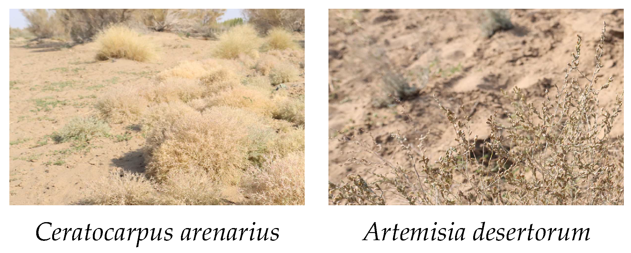
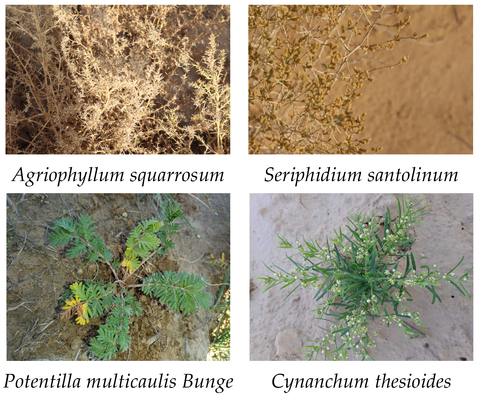
Some plant images from the DGPlant48 dataset are shown in Figure 1, and the complete list of plant species is provided in Table 2.

Figure 1. Representative images from the DGPlant48 dataset illustrating the morphological diversity of desert grassland plants under complex field conditions. Images showcase variations across species, lighting (e.g., harsh noon and soft dusk), capture angles (top-down, side, upward), and background clutter (including soil, shadows, and coexisting vegetation), thereby underscoring the recognition challenges addressed in this study.

Table 2. Plant information statistics of DGPlant48 dataset.

Serial Number	Plant Name	Quantity/Piece	Serial Number	Plant Name	Quantity/Piece	Serial Number	Plant Name	Quantity/Piece
1	Aster altaicus Willd	428	2	Medicago ruthenica	484	3	Astragalus melilotoides	430
4	Plantago depressa Willd	464	5	Dracocephalum peregrinum	468	6	Cynanchum thesioides	434
7	Potentilla multicaulis Bunge	460	8	Peganum multisectum	416	9	Potentilla bifurca	394
10	Limonium bicolor	496	11	Amaranthus retroflexus	404	12	Glycyrrhiza uralensis	401
13	Artemisia gansuensis	510	14	Lycium barbarum	460	15	Lactuca tatarica	406
16	Cynanchum komarovii	514	17	Agropyron mongolicum Keng	504	18	Cynanchum hancockianum	518
19	Lespedeza potaninii	512	20	Thermopsis lanceolata	480	21	Taraxacum mongolicum	402
22	Olgaea leucophylla Iljin	422	23	Euphorbia kozlovii	406	24	Plantago minuta	407
25	Lespedeza daurica	414	26	Malva pusilla	398	27	Stipa bungeana	506
28	Lxeris chinensis	418	29	Salsola collina	514	30	Nitraria tangutorum	408
31	Petrosimonia sibirica	450	32	Tamarix chinensis	510	33	Salsola ferganica	512
34	Karelinia caspia	440	35	Suaeda heteroptera	515	36	Ceratocarpus arenarius	465
37	Suaeda glauca	517	38	Alhagi sparsifolia	447	39	Krascheninnikovia ceratoides	400
40	Reaumuria songonica	500	41	Aristida tsangpoensis	515	42	Calligonum mongolicum	435
43	Artemisia desertorum	436	44	Seriphidium santolinum	510	45	Agriophyllum squarrosum	452
46	Ephedra distachya	475	47	Haloxylon ammodendron	492	48	Halocnemum strobilaceum	505

2.1.2. Data Augmentation

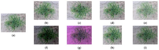
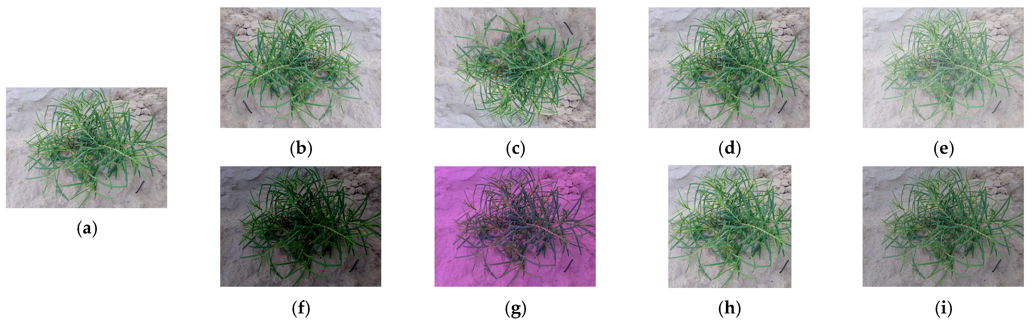
To enhance robustness against environmental variations, we applied eight augmentation techniques simulating field conditions: horizontal/vertical flipping, Gaussian noise, brightness/saturation transformation, center cropping, and salt and pepper noise (low/high intensity). These augmentations addressed perspective changes, lighting fluctuations, electronic noise, weather effects (sandstorms), and partial occlusion. Figure 2 illustrates representative augmentations for Cynanchum thesioides.

Figure 2. Examples of the effects of original images and eight offline data augmentation techniques. (a) Original image, (b) horizontal flip, (c) vertical flip, (d) Gaussian noise, (e) brightness transformation (±30%), (f) saturation transformation (±40%), (g) center cropping (80% of original), (h) low-intensity salt and pepper noise (density = 0.01), (i) high-intensity salt and pepper noise (density = 0.05).

2.2. Teacher Model Design (YOLOv11-STC)

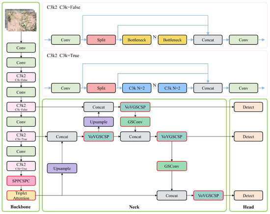
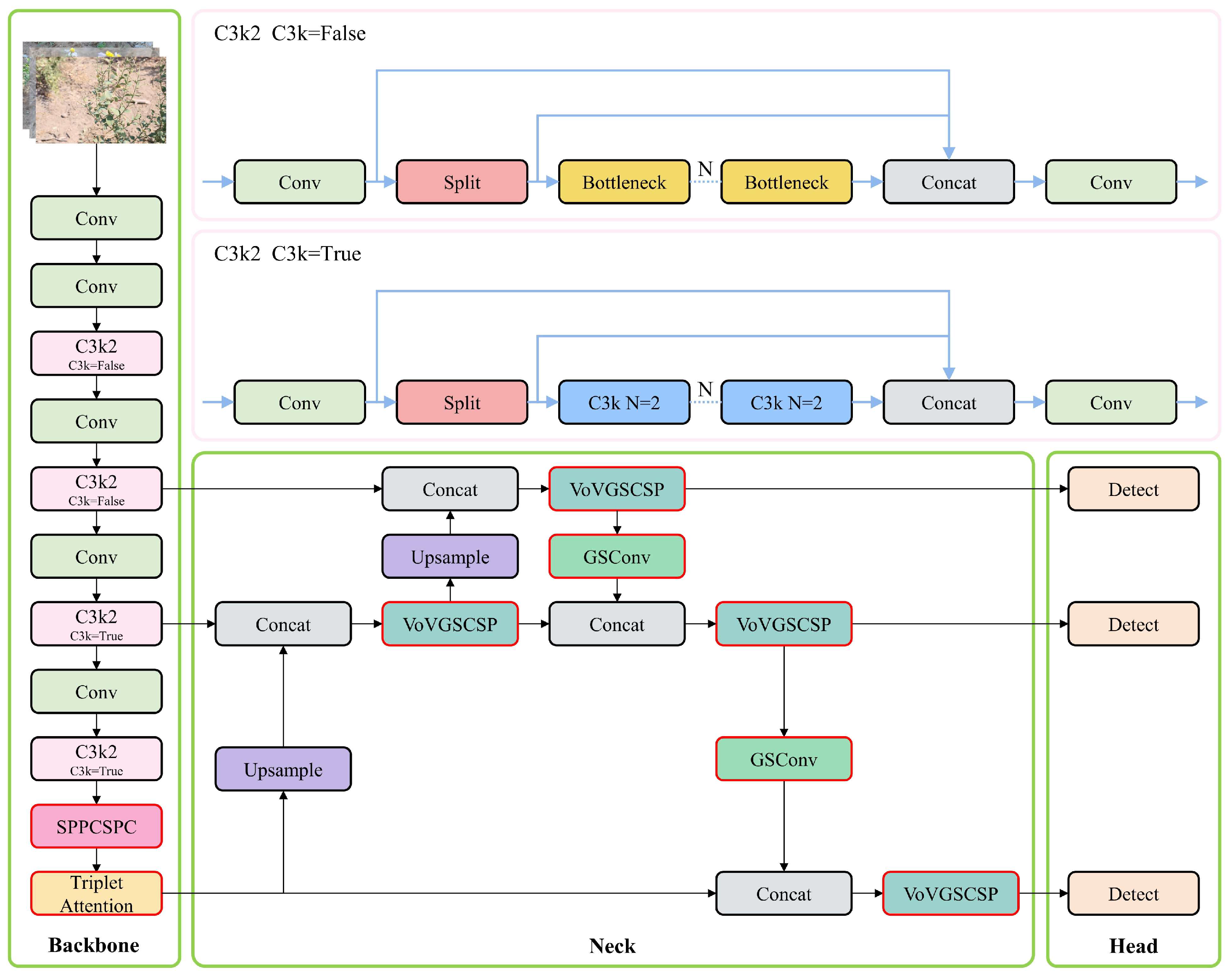
We select YOLOv11n (Ultralytics, v8.3.0) as our baseline—a recent community-validated release that advances the YOLO family through enhanced gradient flow in the Backbone and optimized feature fusion in the Neck, while preserving the single-stage detection paradigm. Its selection is motivated by four key attributes: (1) established balance between accuracy and real-time efficiency; (2) mature lightweight variants suitable for edge deployment; (3) robust ecosystem support for pruning and distillation workflows; and (4) proven effectiveness in agricultural vision tasks under complex field conditions. To address the unique challenges of desert grassland environments, we develop YOLOv11-STC through three synergistic architectural improvements; its structure is illustrated in Figure 3.

Figure 3. YOLOv11-STC overall architecture: Backbone introduces SPPCSPC to enhance multi-scale features, Neck uses Slim Neck to optimize fusion efficiency, and Head integrates Triplet Attention to suppress complex background interference, comprehensively improving the accuracy and robustness of desert grassland plant detection. The improved module has a red border.

As shown in Figure 3, the YOLOv11-STC architecture consists of three main components: the Backbone for feature extraction from input plant images, the Neck for multi-scale feature fusion, and the Head for regression-based prediction.

To enhance the model’s detection performance in complex environments, several key improvements are made: First, the SPPF module in the Backbone is replaced with the more advanced SPPCSPC module [30], which improves the model’s ability to perceive targets across multiple perspectives and scales. Second, the Triplet Attention mechanism [31] is introduced in place of the original C2PSA structure, enabling more effective capturing of global contextual information and improving feature attention in visually complex backgrounds. Finally, the Slim Neck module [32] replaces the standard convolutional layers in the Neck, optimizing multi-scale feature fusion while reducing computational overhead and preserving rich contextual features.

2.2.1. SPPCSPC Module Optimization Detection Layer

The natural environment in which desert grassland plant images are collected is highly complex and variable. Differences in camera height and shooting angles can result in compressed, distorted, or visually diminished target appearances, increasing the likelihood of model misclassification. To enhance the model’s multi-scale feature representation capability, we replace the SPPF module in the original YOLOv11n Backbone with the SPPCSPC module. As illustrated in Figure 4, the SPPCSPC module integrates the spatial pyramid pooling (SPP) [33] and Cross-Stage Partial Connection (CSP) [34] mechanisms into a unified structure [35].

Figure 4. Schematic of the SPPCSPC module integrated into the YOLOv11n Backbone. The module combines spatial pyramid pooling (SPP) with kernel sizes 5 × 5, 9 × 9, and 13 × 13 to capture multi-scale features, and a Cross-Stage Partial (CSP) Connection to split the feature map, reducing computational redundancy while enhancing gradient flow, thereby improving scale-invariant feature extraction for desert plants.

The SPP component applies parallel max pooling operations with three different kernel sizes (5 × 5, 9 × 9, 13 × 13) to extract multi-scale features. The CSP structure splits the feature map into two parts, processing one part through the SPP branch and then concatenating it with the other bypass part. This design improves gradient flow while reducing computational redundancy. It performs spatial pyramid pooling through three independent pooling layers with differently sized kernels, and the formula is provided as follows:

$$R(F^{\prime })=MaxPoo{l}_{k=5}^{p=2}(F_2^{\prime })\otimes MaxPoo{l}_{k=9}^{p=4}(F_2^{\prime })\otimes MaxPoo{l}_{k=13}^{p=6}(F_2^{\prime })$$

(1)

where $MaxPool$ indicates max pooling, $k$ denotes the pooling kernel size, $p$ corresponds to padding parameters, $R$ refers to the output features after multi-scale fusion, and $F$ signifies the input feature map.

2.2.2. Triplet Attention Mechanism

In desert grassland plant detection, certain plant species often blend with the surrounding background, leading to missed or false detections. To address this, we incorporate the Triplet Attention mechanism into the C2f modules of the Backbone network, replacing the standard attention mechanisms. As shown in Figure 5, Triplet Attention employs a three-branch structure to capture cross-dimensional dependencies with minimal computational overhead.

Figure 5. Architecture of the Triplet Attention mechanism. The three branches capture cross-dimensional interactions between channel height and channel width, alongside standard spatial (H-W) attention, using Z-Pool and 7 × 7 convolutions to generate attention weights. This design suppresses background noise in complex desert scenes and directs the model’s focus to critical plant regions.⊙ represents convolution; ⊕ represents summation.

As illustrated in Figure 5, the Triplet Attention module consists of three branches, each receiving input tensors for parallel processing. The first two branches are designed to capture dependencies between spatial and channel dimensions, while the third branch focuses on spatial feature dependencies. In the first two branches, the input tensor is rotated and processed using max pooling and average pooling operations along the 0th dimension to reduce computational complexity while preserving essential feature information. The corresponding operation is defined as:

$$Z-Pool(X)=[MaxPoo{l}_{0d}(X),AvgPoo{l}_{0d}(X)]$$

(2)

Here, $0d$ is the 0th dimension where maximum and average pooling operations occur. The output tensor Y of the Triplet Attention module, given the input tensor $X$, is computed as follows:

$$y={\displaystyle \frac{1}{3}}(\overline{x_1\sigma (\psi (x_1^{\prime }))}+\overline{x_2\sigma (\psi (x_2^{\prime })}+x\sigma (\psi (x_3)))$$

(3)

where $\sigma$ represents the Sigmoid activation function and $\psi$ represents the convolution operation. By capturing these cross-dimensional interactions, Triplet Attention enables the model to more effectively focus on key plant regions while suppressing irrelevant background clutter, significantly improving detection accuracy in complex natural environments.

2.2.3. Slim Neck Paradigm Design

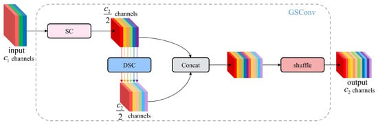
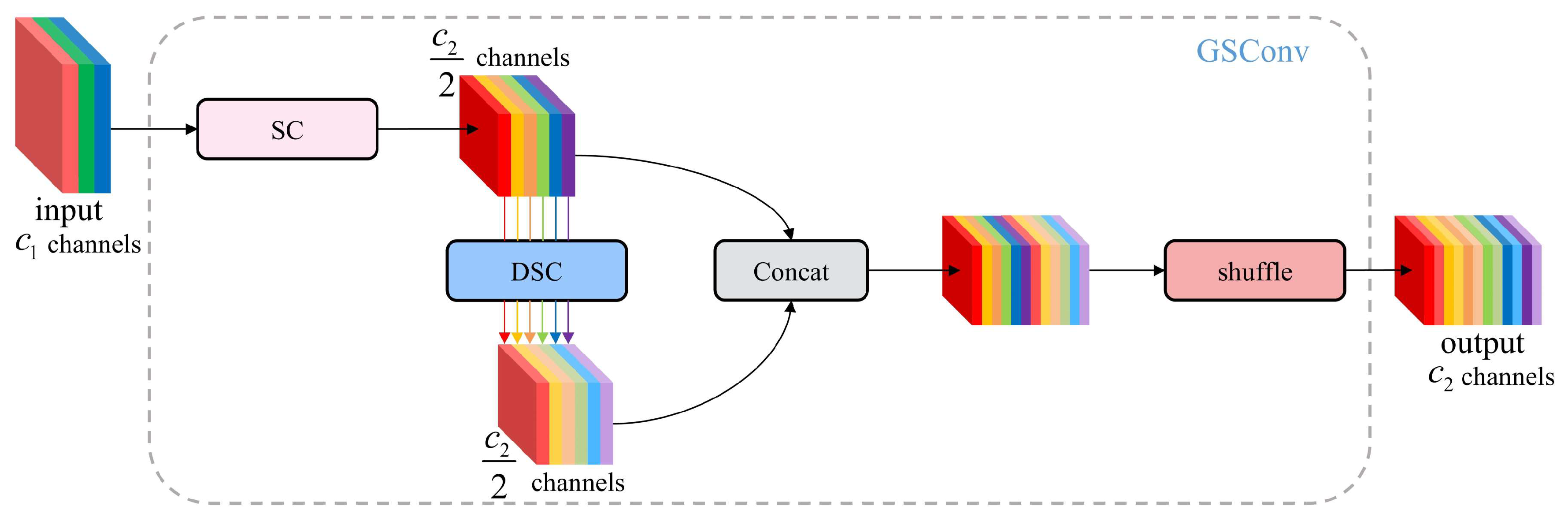
In desert grassland plant images, the diversity of plant morphology and the presence of complex, cluttered backgrounds pose significant challenges for accurate detection. To address this, YOLOv11n incorporates the Slim Neck module, which integrates two optimized components, i.e., GSBottleneck and VOV-GSCSP, built upon the GSConv framework. This design significantly enhances detection accuracy while preserving real-time inference speed. GSConv is a new lightweight convolution which deviates from the conventional strategy of improving accuracy by deepening network structures and increasing computational load. Instead, it achieves higher accuracy through structural optimization without incurring substantial computational cost. GSConv splits standard convolutions into depthwise separable convolutions (reducing computational complexity) and channel shuffling (enhancing feature interaction), similar to “drawing richer details with fewer brushes”, thereby reducing computational costs while maintaining accuracy. The network structure of GSConv is shown in Figure 6.

Figure 6. GSConv network structure: By optimizing computational efficiency through depthwise separable convolution and channel shuffling, the accuracy of desert plant feature extraction is improved.

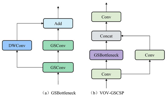
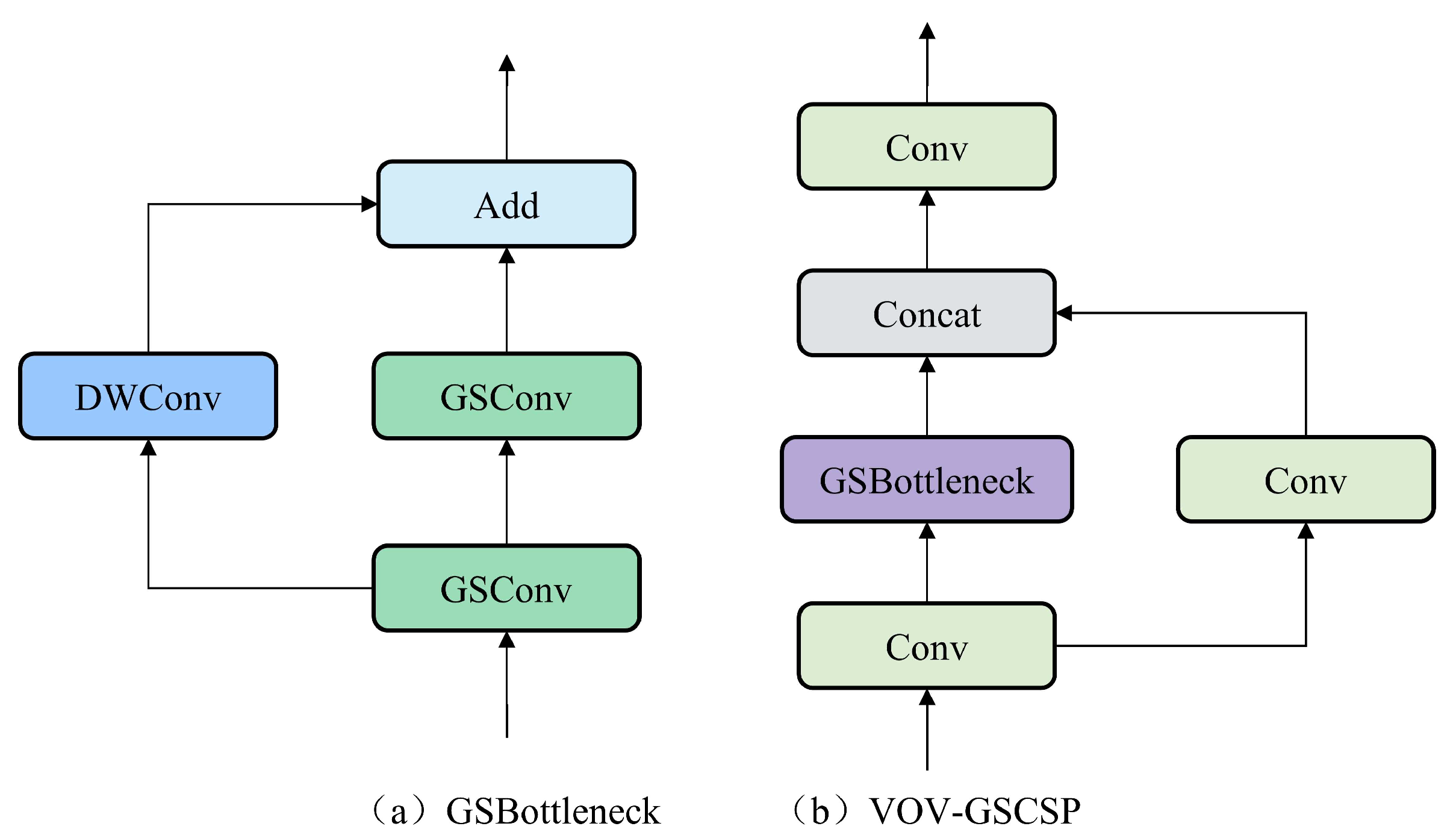
As illustrated in Figure 6, the input features are first processed through a standard convolutional layer, followed by depthwise separable convolutions applied independently to each channel. The output features are then concatenated and passed through a channel shuffle operation to enhance inter-channel information exchange and improve feature representation. The GSBottleneck structure builds upon GSConv by further optimizing its feature processing capabilities, thereby enhancing the model’s ability to extract and refine meaningful features. Meanwhile, VOV-GSCSP adopts a one-time aggregation strategy to streamline the design of specific modules, improving both feature utilization efficiency and overall architectural coherence. Its structure is shown in Figure 7.

Figure 7. GSBottleneck structure and VOV-GSCSP structure.

The Slim Neck structure, shown in Figure 7, allows GSConv to maintain low computational complexity while preserving inter-channel connectivity. It combines the speed advantages of depthwise separable convolution and the representational accuracy of standard convolution. This design significantly improves the model’s ability to recognize desert grassland plants by enhancing its capacity to process images where plant structures are intertwined with complex backgrounds. Consequently, Slim Neck effectively addresses the challenge of detecting morphologically diverse plant species in natural environments.

While YOLOv11-STC achieves superior accuracy (88.3% mAP50), its computational demands (66.3 GFLOPS, 51.0 MB) exceed mobile constraints, necessitating model compression.

2.3. Model Pruning Strategy (Student Model YOLOv11-Pruned)

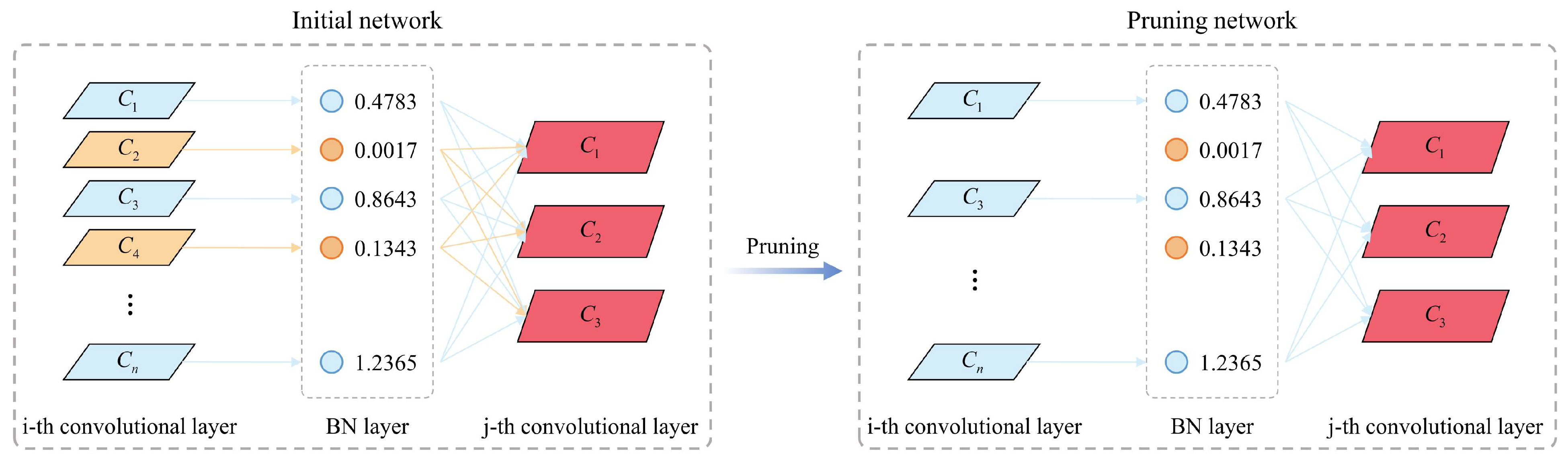
To achieve model lightweighting and accelerate inference speed, this study uses a channel pruning method based on structured pruning techniques [36] to compress the model. Specifically, the Batch Normalization (BN) scaling factors in YOLOv11n are used as the pruning indicators. During the network training phase, L1-regularized sparse training is first applied to the BN scaling factor, encouraging sparsity and enabling the model to automatically identify channels with near-zero scaling values—i.e., channels that contribute minimally to the model’s learning capacity. Following sparse training, channels with smaller scaling factors are pruned, resulting in a more compact and efficient model. The pruned model is then fine-tuned to optimize performance. The overall channel pruning process is shown in Figure 8.

Figure 8. Channel pruning process based on BN scaling factor sparsity: Automatic recognition and pruning of redundant channels (scaling factor approaching 0) driven by regularization, achieving YOLOv11n model compression.

Sparse Training: We first induce sparsity by applying L1 regularization to BN scaling factors during training. The modified loss function combines standard detection loss with a sparsity penalty:

$$L={\displaystyle \sum _{(x,y)}l(f(x,W),y)}+\lambda {\displaystyle \sum _{\gamma \in \mathrm{\Gamma }}g(\gamma )}$$

(4)

$$Y=\underset{\gamma \to 0}{\lim }\gamma ·{\displaystyle \frac{X-\mu }{\sqrt{{\sigma }^2+\epsilon }}}+\beta =\beta$$

(5)

where $(x,y)$ represents the input and target of the training sample, $W$ represents the model weights used in standard training, ${\displaystyle \sum _{(x,y)}l(f(x,W),y)}$ represents a loss term for normal training, ${\displaystyle \sum _{\gamma \in \mathrm{\Gamma }}g(\gamma )}$ is the L1 regularization term applied to the BN scaling factor to encourage sparsity, $\gamma$ is the scaling factor of the BN layer, $\lambda$ is the sparsity regularization coefficient that balances the normal loss and the sparsity penalty, $X$ represents the input sample, $\mu$ represents the data mean, $\sigma$ represents the data standard deviation, $\epsilon$ is a small constant added to the denominator to avoid division by zero, and $\beta$ is the trainable affine transformation parameters.

Channel Pruning: Following sparse training, we rank channels by their BN scaling factor magnitudes and prune those approaching zero. These channels contribute minimally to model output, and their removal effectively compresses the network. We experimentally determine a 35% pruning rate as the optimal balance between model compactness and accuracy retention.

Fine-tuning: The pruning process inevitably leads to a loss in model accuracy, necessitating retraining and fine-tuning to better adapt to the modified network structure and restore performance. To this end, the original dataset and corresponding configuration files are reloaded, the training epochs are set to 200, and the pruned weight file is used to initialize the network for fine-tuning and retraining.

Although pruning effectively reduces model size, the resulting accuracy drop (79.5% vs. 81.5% mAP50) requires performance recovery through knowledge distillation.

2.4. Knowledge Distillation Strategy (Final Student Model YOLOv11-PKD)

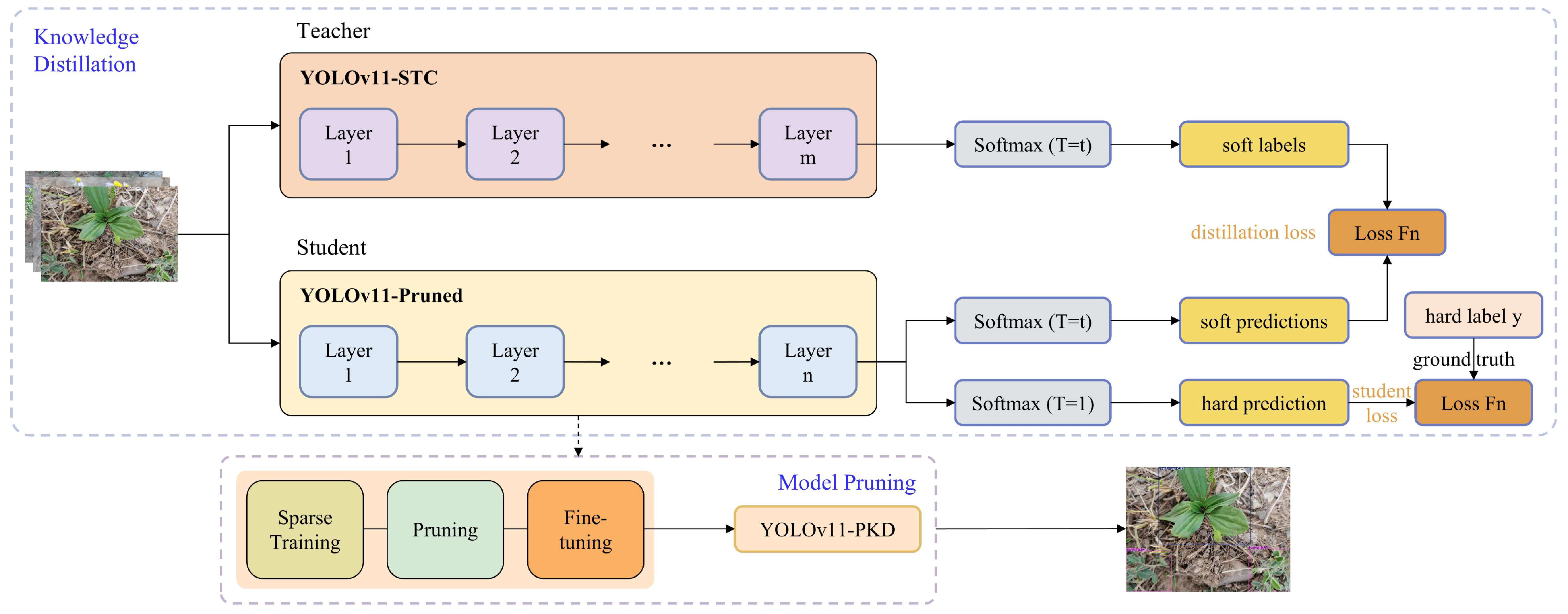
To recover accuracy degradation from pruning, we employ logit-based knowledge distillation to transfer “dark knowledge” [37] from the high-capacity teacher model (YOLOv11-STC) to the compressed student model (YOLOv11-Pruned). The distillation framework (Figure 9) leverages temperature-scaled Softmax outputs to generate soft labels that encode inter-class similarity information [38].

Figure 9. Workflow of the L2-based knowledge distillation framework. The high-capacity YOLOv11-STC teacher model generates soft labels using a temperature-scaled ($T=4$) Softmax function. These soft labels, containing ‘dark knowledge’ of inter-class relationships, guide the training of the lightweight YOLOv11-Pruned student model via a distillation loss ($L_{distill}$), which is combined with the standard detection loss ($L_{detect}$) to form the total training objective.

Temperature-Scaled Softmax: In knowledge distillation, a temperature parameter $T$ is introduced into the Softmax function to soften probability distributions:

$$Softmax(z_i)={\displaystyle \frac{exp(\frac{z_i}{T})}{{\displaystyle {\sum }_{j}exp(\frac{z_i}{T})}}}$$

(6)

where $z_i$ represents the logits and $T$ denotes the temperature coefficient. A higher $T$ value smooths the Softmax output, resulting in a more uniform probability distribution across categories. This smoothness helps retain inter-class similarity information.

Higher $T$ values produce smoother distributions, revealing inter-class relationships that guide the student model’s learning. Through systematic validation on $T\in [1,10]$, we determine $T=4$ as optimal—lower temperatures provide insufficient softening, while higher temperatures over-smooth and dilute informative class relationships.

Distillation Loss Function: The total training objective combines standard detection loss with L2-based distillation loss:

$$L_{total}(x;W)=\alpha \ast L_{detect}(y,\sigma (z_s;T=1))+\beta \ast L_{distill}(\sigma (z_t;T=\tau ),\sigma (z_s,T=\tau ))$$

(7)

where $x$ represents the input image, $W$ denotes the student model’s parameters, $y$ is the ground-truth label, $\sigma$ represents the temperature $T$ parameterized Softmax function, and $z_s$ and $z_t$ represent the logits of the student network and the teacher network, respectively. $L_{detect}$ is the standard detection loss (e.g., cross-entropy and CIOU loss) between the student’s hard predictions (with temperature $T=1$) and the ground truth. $L_{distill}$ is the distillation loss, computed using the L2 distance between the softened logits of the teacher ($z_t$) and the student ($z_s$) at a specified temperature $T=\tau$. The coefficients $\alpha$ and $\beta$ are weighting factors that balance the contributions of the two loss terms. Through empirical validation, we set $\tau =4$, $\alpha =0.7$, and $\beta =0.3$ to achieve optimal knowledge transfer without overshadowing the task-specific supervisory signal.

Distillation Method Selection: We systematically evaluated three logit-based distillation strategies to identify the optimal approach for performance recovery:

• L1 distance (Manhattan distance) [39]: Minimizes absolute differences between student and teacher logits, emphasizing fine-grained distinctions.
• L2 distance (Euclidean distance) [39]: Minimizes squared differences, penalizing large deviations more heavily to align overall output distributions.
• BCKD (Classifier-Based Knowledge Distillation) [40]: Trains an intermediary classifier on teacher outputs to guide student learning indirectly.

We systematically assess sensitivity to this hyperparameter by testing multiple weight configurations during validation. We select L2 distillation based on its theoretical suitability for pruned model recovery: the squared error property smooths logit variations while imposing stronger penalties on significant deviations from teacher predictions. This characteristic effectively restores feature representations compromised during channel pruning, without requiring auxiliary classifier training (BCKD) or fine-grained absolute difference optimization (L1). The final weighting coefficients (α = 0.7, β = 0.3) and temperature (T = 4) are determined via grid search on the validation set to optimize the accuracy–efficiency trade-off.

2.5. Model Evaluation Indicators

In this study, multiple performance evaluation metrics were used to comprehensively evaluate the performance of the model, including precision (P), recall (R), average precision (AP), and Mean Average Precision (mAP). The specific definitions are as follows:

The formula for calculating precision (P) is:

$$P={\displaystyle \frac{TP}{TP+FP}}$$

(8)

The formula for calculating the recall rate (R) is:

$$R={\displaystyle \frac{TP}{TP+FN}}$$

(9)

The average precision (AP) calculation formula is:

$$AP={\displaystyle {\int }_0^{1}P(R)dR}$$

(10)

Mean Average Precision (mAP) is the average AP value of all categories (c), calculated as:

$$mAP={\displaystyle \frac{1}{c}}{\displaystyle \sum _{i=1}^{c}A{P}_i}$$

(11)

Among them, $TP$ represents true positive, $TN$ represents true negative, $FP$ represents false positive, and $FN$ represents false negative, which are used to calculate accuracy and recall. $AP$ is obtained by calculating the area under the corresponding precision–recall (P-R) curve.

To comprehensively evaluate the extent of model lightweighting, this study adopts three key metrics: model size (disk space usage), number of model parameters (Parameters), and floating-point operations (GFLOPS). Model size refers to the memory footprint of the model, including the storage required for weight and bias parameters. Parameters denote the total number of trainable parameters in the network, reflecting the model’s complexity. GFLOPS measures the computational cost by quantifying the number of floating-point operations needed during a single forward pass or training iteration. These metrics collectively provide an effective assessment of the model’s efficiency and suitability for deployment in resource-constrained environments.

To ensure robustness, 5 independent training runs were conducted per model with different random seeds (42, 123, 456, 789, 1011). The paired t-test was performed by pairing per-class AP values (n = 48 classes) between model pairs within each run (e.g., YOLOv11-STC vs. YOLOv11n, run 1; YOLOv11-STC vs. YOLOv11n, run 2), yielding 5 paired observations per class comparison. Assumption verification: Normality of AP differences was confirmed via the Shapiro–Wilk test (W > 0.95, p > 0.05); homoscedasticity was verified by Levene’s test (p > 0.05). A p-value <0.05 was considered statistically significant and p < 0.01 highly significant.

2.6. Experimental Environment Setup

All models were trained and evaluated on the same hardware platform, which consisted of a Windows 11 operating system, an Intel (R) Core (TM) i9-14900K CPU, an NVIDIA GeForce RTX 4090D 24 GB GPU, and 128 GB of DDR5 RAM. The training environment was configured using PyTorch 2.5.1, Python 3.9.13, and CUDA 12.4.

To ensure a fair and comprehensive evaluation, all comparative and ablation experiments were conducted under identical training protocols on the DGPlant48 dataset. Training was conducted for 200 epochs with a batch size of 16, and input images were resized to 640 pixels × 640 pixels. Hyperparameters, including the initial learning rate, optimizer, and number of training epochs, were determined through a grid search on the validation set to optimize performance across all models. The selection of baseline models (YOLOv3n to YOLOv11n) was made to represent the evolution of the YOLO family, focusing on lightweight versions suitable for potential mobile deployment. Furthermore, the statistical significance of performance differences reported in comparative studies was validated using a paired t-test on per-class average precision (AP) values from multiple independent runs, with a p-value <0.05 considered statistically significant.

2.7. Mobile Application Development

To verify the practical applicability of the proposed model, we develop a mobile plant identification app for desert grassland species [41,42]. The deployment pipeline involves: (1) PyTorch to ONNX conversion (opset = 12) using ultralytics export; (2) FP16 quantization via ONNX Runtime quantization tools; and (3) deployment on ONNX Runtime Mobile v1.15.0 with XNNPACK delegate for CPU acceleration. The system employs a Flask-based backend server to host the recognition service, whereas the mobile client is developed with the Uni-App framework to support image capture and recognition result display. Users can capture images in real time or upload photos from their gallery, with the system returning species identification and detailed plant information within ~1 s. This architecture supports model hot-updates and collects user feedback, facilitating continuous model improvement and database expansion. The real-time response and user-interactive design of the app further validate the practical value of the proposed model in resource-constrained mobile scenarios.

Mobile Test Environment: Inference latency was benchmarked on three representative devices: (a) Xiaomi Mi 10 (Snapdragon 865, 8 GB RAM, Android 12) as the mid-tier reference; (b) Samsung Galaxy S21 (Exynos 2100, 8 GB RAM, Android 13) for cross-platform validation; and (c) Redmi Note 9 (MediaTek Helio G85, 4 GB RAM, Android 11) for low-end compatibility. All tests used single-threaded inference with batch_size = 1, input resolution 640 × 640, and 4 warm-up runs preceding 100 timed iterations. Network latency was excluded by running the Flask server on local WiFi (ping < 5 ms).

3. Results and Discussion

3.1. Teacher Model Analysis

3.1.1. Comparative Experiments of Different Models

To comprehensively evaluate the effectiveness and advantages of the proposed YOLOv11-STC model, comparative experiments were performed on the DGPlant48 dataset, where the model was compared with several mainstream lightweight YOLO variants, including YOLOv3n, YOLOv5n, YOLOv8n, YOLOv9m, YOLOv10n, and YOLOv11n. All models were trained and tested under consistent hyperparameter configurations to guarantee the fairness of the comparison. The recognition performance of each model is summarized in Table 3.

Table 3. Comparative results of different network models on the DGPlant48 dataset.

Model	P/%	R/%	mAP50/%	GFLOPS/G	Model Dimension/MB	Parameters/M
YOLOv3n	80.3	74.1	81.1	282.4	207.8	10.370
YOLOv5n	78.1	73.5	80.3	7.1	5.3	2.512
YOLOv8n	78.5	76.3	82.2	8.1	6.3	3.015
YOLOv9m	80.4	75.8	81.9	76.7	40.9	2.004
YOLOv10n	76.7	75.3	80.1	8.3	5.8	2.713
YOLOv11n	79.5	72.5	81.5	6.5	5.5	2.592
YOLOv11-STC	85.4	83.2	88.3	66.3	51.0	25.282

Note: Bold data indicate the best performance under the respective metric. The significance of the difference in mAP50 between the proposed YOLOv11-STC model and all other baseline models was assessed using a paired t-test. Paired t-tests were conducted on per-class AP values (48 classes) across five independent runs (seeds: 42, 123, 456, 789, 1011). For each model pair comparison, n = 5 paired observations were made (mean AP per run). All comparisons satisfied normality (Shapiro–Wilk p > 0.05) and homoscedasticity assumptions. Exact p-values: p < 0.05, p < 0.01. The results indicate that the performance improvement achieved by YOLOv11-STC is statistically significant, with a p-value <0.01.

The YOLOv11-STC model outperformed the YOLOv3n, YOLOv5n, YOLOv8n, YOLOv9m, YOLOv10n, and YOLOv11n models by 7.2%, 8.0%, 6.1%, 6.4%, 8.2%, and 6.8%, respectively, in mAP50. However, this performance gain comes at the cost of increased computational demands. Specifically, the YOLOv11-STC model exhibits large values in model size, Parameters, and GFLOPS, indicating a higher demand for hardware resources. The model size of YOLOv11-STC is 51.0 MB, which is considerably larger than those of the lightweight baselines—YOLOv5n (5.3 MB), YOLOv8n (6.3 MB), YOLOv10n (5.8 MB), and YOLOv11n (5.5 MB)—but smaller than YOLOv3n (207.8 MB) and YOLOv9m (40.9 MB). It contains 25.3 M parameters —more than double those of the comparison models, none of which exceed 10.4 million. In terms of computational cost, YOLOv11-STC reaches 66.3 GFLOPS, which is higher than most models, second only to YOLOv3n.

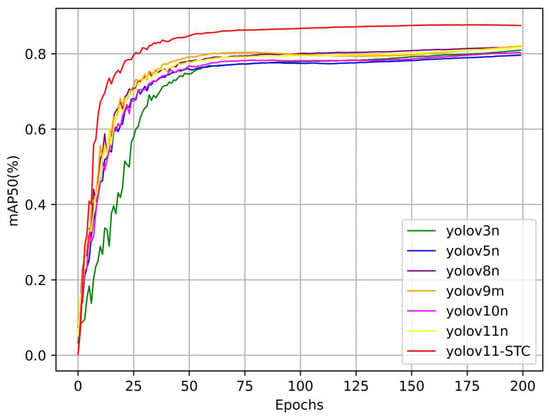
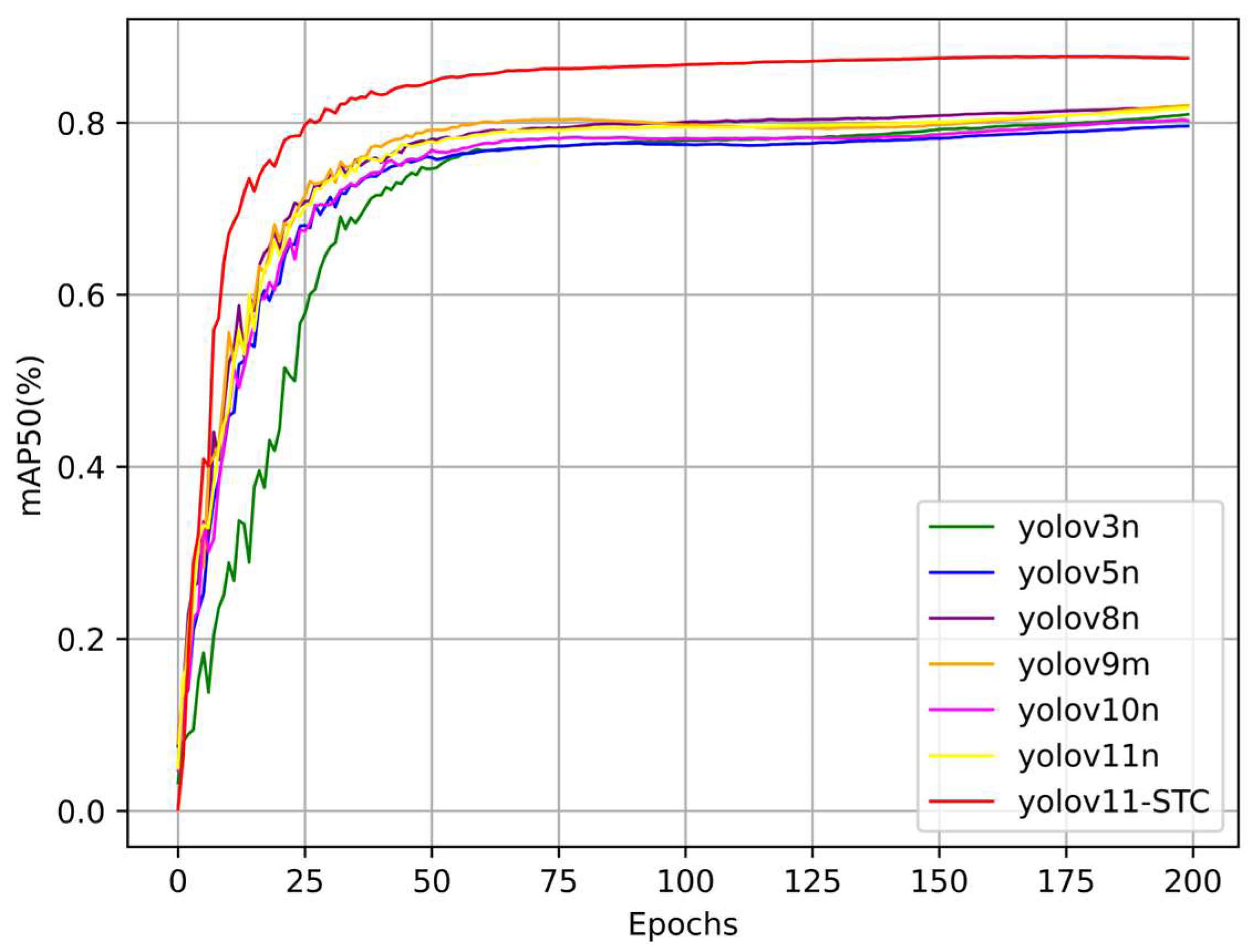
To more intuitively illustrate the performance of each model during training, the mAP50 progression curves were plotted for all models, as shown in Figure 10. The mAP50 curve of the YOLOv11-STC model consistently remains above those of the comparison models and rises rapidly during the initial training phase, ultimately stabilizing at a higher value. This demonstrates that YOLOv11-STC achieves faster convergence and superior final performance. In contrast, while the curves of other models also show an upward trend, they generally remain at a lower level. Some even exhibit noticeable fluctuations or slower growth in the later stages of training, highlighting the stability and performance advantage of the YOLOv11-STC model throughout the training process.

Figure 10. mAP50 progression curves of different models during training. The curves illustrate the Mean Average Precision at IoU = 0.5 across training epochs for YOLOv11-STC and baseline models. Each curve represents the moving average of mAP50 values over five independent training runs.

3.1.2. Analysis of Ablation Experiment

To further investigate the individual contributions of each component in the YOLOv11-STC model to the accuracy and performance of plant recognition in desert grasslands, ablation experiments were conducted using a controlled variable approach. The results are presented in Table 4.

Table 4. Ablation study results of YOLOv11-STC components on the DGPlant48 dataset.

Experiment	SPPCSPC	Triplet Attention	GSConv	P/%	R/%	mAP50/%	GFLOPS/G	Parameters/M	Model Dimension/MB
Baseline	×	×	×	79.5	72.5	81.5	6.5	2.592	5.5
A	√	×	×	81.3	77.4	83.6	73.5	26.486	53.5
B	×	√	×	79.6	75.2	82.9	68.3	19.869	40.2
C	×	×	√	84.0	79.7	84.5	61.8	19.050	38.6
D	√	√	×	83.3	80.4	86.2	72.9	26.318	53.1
E	×	√	√	83.6	80.1	85.9	61.7	18.853	38.1
F	√	×	√	85.4	83.2	87.8	67.0	25.479	51.4
G	√	√	√	87.0	84.2	88.3	66.9	25.282	51.0

Note: Bold data indicate the best performance under the respective metric. ”√” indicates that this module is included, “×” indicates that this module is not included.

The non-monotonic parameter trends observed in Table 4 (e.g., Experiment A: 26.486 M to D: 26.318 M to G: 25.282 M) arise from the specific architectural implementations of the integrated modules. Unlike standard additive ablation studies where modules simply stack upon the baseline, our modifications involve both parameter-increasing and parameter-reducing operations: (1) SPPCSPC introduces additional parameters through its multi-scale pooling branches (parameter increase); (2) Triplet Attention replaces the original C2PSA module rather than adding to it, resulting in a more efficient attention mechanism (parameter reduction); and (3) GSConv-based Slim Neck substitutes standard convolutions with depthwise separable convolutions and channel shuffling, significantly compressing the Neck section (parameter reduction). Consequently, when these efficiency-oriented modules (Triplet Attention and GSConv) are combined with capacity-adding modules (SPPCSPC), the net effect is a gradual reduction in total parameters while maintaining or improving accuracy. This synergistic optimization—adding representational capacity while removing computational redundancy—demonstrates the effectiveness of our architectural design strategy.

Experiment A shows notable improvements in precision (P), recall (R), and mAP50, but these gains come with significantly increased GFLOPS and model size. This indicates that while the corresponding module can effectively enhance performance, it introduces substantial computational overhead. In contrast, Experiment B achieves only marginal improvements in performance, despite increased computational cost and model size, suggesting that this module performs suboptimally when used in isolation. Experiment C delivers substantial improvements across all performance metrics while maintaining relatively low computational complexity and model size. This underscores the module’s balanced advantage in enhancing recognition accuracy without imposing excessive resource costs.

Experiments D, E, and F explore combinations of modules. These configurations yield further performance gains, with Experiment F achieving high P (85.4%), R (83.2%), and mAP50 (87.8%) values. Moreover, it maintains a relatively balanced profile in terms of computational demands and model size, making it a practical choice in resource-constrained environments. Experiment G, which integrates all three modules, achieves the best overall performance: P of 87.0%, R of 84.2%, and mAP50 of 88.3%. Although its GFLOPS (66.9 G), parameter count (25.282 M), and model size (51.0 MB) are higher than some individual configurations, they remain within acceptable bounds. The synergistic combination of modules enables the YOLOv11-STC model to reach peak recognition capability while maintaining reasonable computational requirements.

In summary, the proposed YOLOv11-STC model demonstrates superior performance across all key metrics (P, R, mAP50) for desert grassland plant identification. However, its increased resource consumption suggests that model compression or lightweighting techniques may be necessary for real-world deployment scenarios.

3.2. Analysis of Model Pruning Effect

3.2.1. Comparison of Model Performance Under Different Pruning Rates

In practical applications, excessive pruning can significantly reduce the model’s recognition accuracy. Therefore, selecting an appropriate pruning ratio is essential to achieve an optimal balance between performance and computational efficiency based on specific performance requirements and resource constraints. For the YOLOv11n model, each layer was evaluated during the pruning process. Starting from a pruning ratio of 20%, five different pruning levels were experimentally tested, and the corresponding model performance was recorded. The comparative results under different pruning ratios are presented in Table 5.

Table 5. Comparison of model performance under different pruning rates.

Pruning Rate	mAP50/%	Parameters/M	GFLOPS/G	Model Dimension/MB
Base	81.5	2.592	6.5	5.5
20%	80.7	2.260	6.0	4.8
35%	78.3	2.153	5.3	4.5
50%	76.5	1.831	4.7	3.8
66%	74.1	1.499	3.9	3.2
80%	71.2	0.956	2.8	2.1

As the pruning ratio increases, Parameters, GFLOPS, and model size all decrease progressively, indicating that pruning effectively reduces the model complexity and storage requirements. Considering both accuracy and model compactness, the pruned model retaining 35% of the original channels is selected as the final model. At this pruning rate, the model achieves a favorable trade-off between recognition accuracy and computational efficiency. This balance can be attributed to two main factors: (1) the removal of redundant parameters that contribute minimally to the model’s output, which simplifies the architecture, enhances sparsity, and improves computational efficiency by reducing unnecessary activations, and (2) the use of structured pruning, which selectively removes less important weights while preserving critical features, thereby maintaining model accuracy even after compression.

In summary, adopting a 35% pruning rate enables effective model compression while preserving accuracy. This layerwise adaptive pruning achieves a favorable trade-off between model compactness and recognition performance, validating its suitability for deployment under resource-constrained environments.

3.2.2. Model Changes After Fine-Tuning

After fine-tuning, the model exhibited a slight decrease in accuracy compared to its pre-pruning performance. The pruned version is referred to as YOLOv11-Pruned, and a detailed comparison of model performance before and after pruning is shown in Table 6.

Table 6. Comparison of models before and after fine adjustment.

Model	P/%	R/%	mAP50/%	GFLOPS/G	Parameters/M	Model Dimension/MB
YOLO v11n	79.5	72.5	81.5	6.5	2.592	5.5
YOLOv11-Pruned	77.5	72.2	79.5	5.2	2.083	4.7

Although the accuracy of the pruned YOLOv11-Pruned model slightly decreased after fine-tuning—reflected by a drop in P from 79.5% to 77.5%, R from 72.5% to 72.2%, and mAP50 from 81.5% to 79.5%—the model achieved notable reductions in complexity and size. Specifically, the GFLOPS decreased by approximately 20%, the number of Parameters was reduced by about 19.7%, and the model size shrank by around 14.5%. These results demonstrate that the fine-tuning process not only preserves the pruned model’s core performance but also significantly improves its computational efficiency and deployability.

In conclusion, when applying an appropriate pruning strategy followed by fine-tuning, the model achieves a favorable trade-off between accuracy and efficiency. This approach effectively reduces the computational burden and storage requirements while maintaining satisfactory recognition performance, enhancing the model’s suitability for deployment in resource-constrained environments.

3.3. Analysis of Knowledge Distillation Effect

3.3.1. The Influence of Different Distillation Methods and Different Loss Weights on the Performance of Student Models

Knowledge distillation loss was used to measure the difference between the predictions of the student model and the teacher model. By adjusting the associated loss weights, the relative importance of different loss terms can be modulated. During the distillation process, it was crucial to align the feature distributions of the intermediate outputs between the student and teacher models while simultaneously minimizing the divergence in their final output probability distributions. This dual constraint enabled the student model to more effectively mimic both the output behavior and internal feature representations of the teacher model, thereby enhancing its ability to learn richer and more efficient representations.

To explore the impact of different distillation methods and loss weight settings on the performance of student models, three logits-based distillation strategies—L1, L2, and BCKD—were evaluated. For each method, comparative experiments were conducted using two different loss weight settings: 0.5 and 1.0. The YOLOv11-Pruned model served as the baseline student model in all experiments. The resulting performance metrics are summarized in Table 7.

Table 7. Comparison of different distillation methods and different loss weights.

Method	Weight	P/%	R/%	mAP50/%	Model Dimension/MB
Pruned	-	77.5	72.2	79.5	4.7
L1	L = 0.5	85.3	82.6	87.2	5.0
	L = 1.0	86.5	82.1	87.6	5.0
L2	L = 0.5	86.7	82.8	87.9	5.0
	L = 1.0	85.3	82.2	87.6	5.0
BCKD	L = 0.5	86.7	82.3	87.8	5.0
	L = 1.0	84.5	82.0	87.5	5.0

Note: L is the loss weight.

The results in Table 7 demonstrate that both the choice of distillation method and the adjustment in loss weight significantly impact model performance. For a given distillation method, tuning the loss weight can further enhance the model’s predictive capability. Under the L1 distillation method, increasing the loss weight from 0.5 to 1.0 improves the mAP50 from 87.2% to 87.6%, though with a slight drop in recall. In contrast, under the L2 method, the lower loss weight (L = 0.5) yields better overall performance, achieving 86.7% precision, 82.7% recall, and 87.9% mAP50—surpassing the results with L = 1.0. Similarly, the BCKD method performs best at L = 0.5, with a strong balance across all metrics: 86.7% precision, 82.3% recall, and 87.8% mAP50. Among all tested configurations, the L2 method with a loss weight of 0.5 provides the most favorable trade-off, delivering the highest mAP50 of 87.9% along with strong precision and recall, while maintaining a compact model size of 5.0 MB. These findings indicate that effective selection of distillation strategy and loss weighting is crucial for optimizing student model performance after pruning.

3.3.2. Comparison of Knowledge Distillation Effects

To evaluate the effectiveness of the distillation process, the model using the L2 distillation method with a loss weight of L = 0.5 was designated as YOLOv11-PKD. Its performance on the test set was compared against the original model (YOLOv11n), the teacher model (YOLOv11-STC), and the student model prior to distillation (YOLOv11-Pruned). To further validate the advantages of our proposed model in terms of the accuracy–efficiency trade-off, we expanded our comparative experiments to include several renowned state-of-the-art (SOTA) lightweight models. Specifically, we compared it against:

MobileNetV3-Small [43]: A classic lightweight Backbone known for its hardware-efficient architecture, which we integrated with a single-shot detection (SSD) Head to ensure fair comparison in object detection tasks.

EfficientNet-Lite0 [44]: A member of the EfficientNet family optimized for mobile and edge devices, where the Lite0 variant is the smallest and achieves a balance between accuracy and efficiency.

NanoDet-Plus: A recently proposed lightweight detection model specifically designed for edge devices, featuring a customized pan-sharpening module and adaptive training strategy.

All comparative models were trained from scratch on the DGPlant48 dataset, adopting the same hyperparameter configurations and training schedules as the proposed models to guarantee comparison fairness. The results are summarized in Table 8.

Table 8. Comparative results of different object detection models on the DGPlant48 dataset.

Model	P/%	R/%	mAP50/%	GFLOPS/G	Parameters/M	Model Dimension/MB
MobileNetV3-Small (SSD)	72.1	68.5	75.3	1.2	2.011	4.9
EfficientNet-Lite0 (SSD)	74.5	70.2	77.8	2.1	3.863	7.9
NanoDet-Plus	76.8	73.6	80.5	3.4	0.954	2.1
YOLOv11n (Our Baseline)	79.5	72.5	81.5	6.5	2.592	5.5
YOLOv11-STC	87.0	84.2	88.3	66.9	25.282	51.0
YOLOv11-Pruned	77.5	72.2	79.5	5.2	2.083	4.7
YOLOv11-PKD (Ours)	86.7	82.8	87.9	5.5	2.150	5.0

Note: The best results are in bold. Our YOLOv11-PKD achieves the highest accuracy among all lightweight models while maintaining competitive model size and computational cost.

As evidenced by the results in Table 8, our final lightweight model, YOLOv11-PKD, demonstrates superior performance. It significantly outperforms all other SOTA lightweight detection models in terms of precision, recall, and most crucially, mAP50. Although models such as NanoDet-Plus have a smaller model size and fewer parameters, and MobileNetV3-Small achieves the lowest computational cost (GFLOPS), they exhibit a significant accuracy gap compared with the proposed method. YOLOv11-PKD strikes a remarkable balance, achieving an mAP50 of 87.9%—which is 5.8 to 12.6 percentage points higher than the other lightweight models—while its model size (5.0 MB) and computational cost (5.5 GFLOPS) remain highly competitive and practical for mobile deployment. This demonstrates the effectiveness of our pruning and distillation strategy in creating a model that excels in both accuracy and efficiency, without forcing a trade-off between them.

3.4. Visualization Analysis of Heatmap

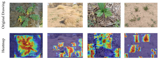
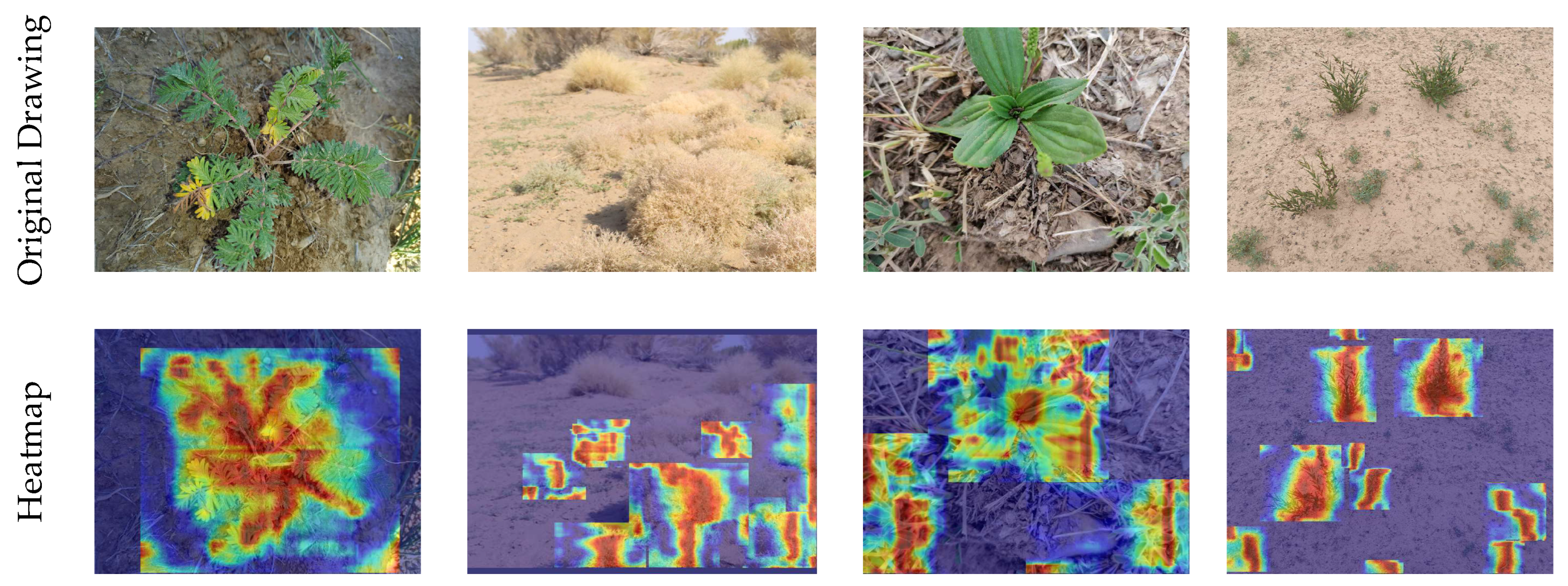
Grad-CAM heatmaps enable intuitive visualization of whether the network has effectively learned key features: they highlight regions of interest via color intensity to reflect the model’s attention distribution. In this study focused on plant recognition in desert grasslands, Grad-CAM was used to visualize and analyze the feature attention of the YOLOv11-PKD model. The resulting heatmaps are presented in Figure 11.

Figure 11. Visualization of heatmap. The top row shows the original input images used for analysis. The middle row displays the corresponding Grad-CAM heatmaps, where color intensity represents the model’s attention to different regions—areas closer to deep red indicate stronger activation responses, highlighting regions that are more influential in the model’s decision-making process. The bottom row illustrates the final detection results, showing the bounding boxes generated by the model.

As shown in Figure 11, the strong alignment between the highlighted regions in the heatmaps and the actual detection outputs suggests that the YOLOv11-PKD model effectively learns and focuses on the most salient features of desert grassland plants. This alignment confirms that the model can not only detect but also accurately localize critical plant structures, thus ensuring reliable performance in practical recognition scenarios.

To assess model robustness across the 48 desert grassland species, we analyzed per-class detection accuracy (Appendix A Table A1). The results reveal substantial performance variation strongly correlated with visual phenotypic traits. Green-leaved species with high contrast (e.g., Medicago ruthenica, mAP50: 99.4%; Aster altaicus, mAP50: 99.5%; and Glycyrrhiza uralensis, mAP50: 93.6%) consistently achieved >90% mAP50, whereas desert-colored species (e.g., Artemisia desertorum, mAP50: 75.9%; Krascheninnikovia ceratoides, mAP50: 55.0%; and Suaeda heteroptera, mAP50: 58.6%) showed significantly degraded performance. This 32.0-percentage-point gap (p < 0.001) confirms that plants with green leaves are much more easily detected, while species with colors and textures similar to the desert background pose substantial challenges.

3.5. Discussion

3.5.1. Key Factors for Improving Model Performance

The YOLOv11-STC teacher model proposed in this study achieved the best recognition accuracy (mAP50: 88.3%) on the DGPlant48 dataset. This performance improvement is mainly attributed to three aspects: firstly, the SPPCSPC module enhances the model’s feature extraction ability for plants at different shooting angles and scales through multi-scale pooling; secondly, the Triplet Attention mechanism enables the model to more accurately focus on the key features of the plant itself, effectively suppressing interference from complex backgrounds; finally, the Slim Neck structure is based on the lightweight design of GSConv, optimizing the feature fusion process without significantly increasing computational costs. The results of the ablation experiment (Table 3) confirmed the synergistic effect of the above modules.

As shown in Table 8, our YOLOv11-PKD model achieved an mAP50 of 87.9%, significantly outperforming other lightweight models such as MobileNetV3-Small (75.3%) and NanoDet-Plus (80.5%). This improvement can be attributed to our combined pruning and distillation strategy, which preserves critical features while reducing redundancy—a challenge noted in recent lightweight detector designs [32,33,34,35,36,37,38,39,40]. Compared to the greenhouse-trained model by Basavegowda et al. [26], which achieved high accuracy under controlled conditions but limited generalization, our model demonstrated robust performance in complex natural scenes, highlighting the importance of in-the-wild data collection and augmentation.

3.5.2. Balancing the Effectiveness of Lightweight Strategies

The combination of model pruning and knowledge distillation has successfully achieved a balance between accuracy and efficiency. Experiments have shown that a pruning rate of 35% is an optimal inflection point which can significantly reduce the model volume and computational complexity while maintaining controllable accuracy loss (mAP50 reduced by 2%). The subsequent knowledge distillation techniques, especially the L2 distillation method (loss weight 0.5), effectively transferred the “dark knowledge” of the teacher model to the lightweight student model, restoring the accuracy of the YOLOv11-PKD model to a level close to that of the teacher model (mAP50: 87.9%), while the model size was only 5.0 MB. This proves the feasibility and superiority of this lightweight strategy for mobile deployment.

3.5.3. Comparison with Existing Research

Compared with the method relying on manual features proposed by Wu et al. [22], which combines contour and appearance descriptors for plant identification, our deep learning-based approach demonstrates stronger feature representation capabilities and better adaptability to complex environmental variations. While Wu et al.’s method achieved robust performance on standardized leaf datasets, it remained sensitive to lighting and background clutter—a limitation effectively mitigated by our multi-scale and attention-enhanced architecture. Similarly, Li et al. [23], evaluated several CNN models under controlled laboratory conditions and identified MobileNetV2 as a suitable lightweight architecture. Moreover, while the use of knowledge distillation in orchard environments reported by Liang et al. [26] aligns conceptually with this study, our approach successfully extends its application to desert grasslands characterized by diverse vegetation forms and complex backgrounds, thereby validating the universality and robustness of the proposed technological framework approach.

3.5.4. Feasibility of Mobile Deployment

Although the teacher model YOLOv11-STC has high computational complexity (66.3 GFLOPS), the combined use of structured pruning and knowledge distillation successfully compress it into the YOLOv11-PKD model, with a size of only 5.0 MB. On Snapdragon 865 (Xiaomi Mi 10), this achieves 1.05 s inference latency—meeting the <2 s threshold for usable field applications. Further optimizations including INT8 quantization reduce latency to 0.89 s but are not deployed due to minor accuracy degradation (86.7% to 85.5% mAP50). The 5.5 GFLOPS computational cost maps to ~180 MB peak memory usage during inference, well within the 4 GB RAM device capabilities.

3.5.5. Limitations and Future Work

Although this study achieved promising results, several limitations remain and warrant further investigation.

(1) Robustness under Extreme Conditions: The model’s performance exhibits fluctuations, with recognition accuracy dropping by 5–8% under extreme weather conditions such as sandstorms, which severely degrade image quality. This indicates a need to enhance the model’s robustness to strong noise interference. Future work will explore advanced data augmentation techniques simulating adverse weather and incorporate image restoration modules to preprocess low-quality inputs.

(2) Dataset Scale and Diversity: The current model is trained and evaluated on 48 plant species primarily from Northwestern China. Despite its representativeness, this scope restricts the model’s global applicability. Future efforts will concentrate on expanding the dataset to encompass a wider range of plant species from other arid and semi-arid regions (e.g., Central Asia), thereby enhancing the model’s generalization ability.

(3) Dependence on RGB Imagery: The model currently relies solely on RGB image data. For species with highly similar morphological characteristics, this modality may lead to a discriminative bottleneck. Integrating multimodal data—such as near-infrared (NIR) channels, multispectral or hyperspectral data capturing leaf biochemical properties, or 3D structural information—could provide complementary features to overcome this limitation.

(4) Exploration of Architectural Alternatives: Future research will also explore the integration of vision transformers (ViTs) [45] or hybrid CNN–Transformer architectures, which may offer superior feature representation for fine-grained plant classification tasks.

4. Application

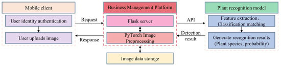
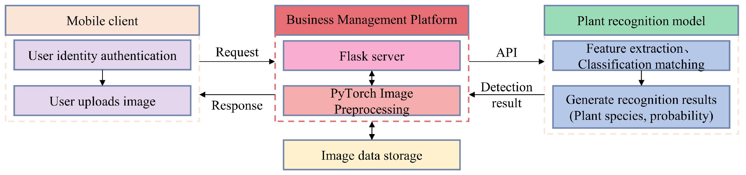
To support the investigation of plant species and their distribution in desert grasslands, as well as to enable real-time tracking of plant growth and morphological traits, this study developed a mobile-based plant image recognition application built on the YOLOv11-PKD model. The application was developed using the Uni-App framework combined with the Android HBuilder tool and leveraged the cloud packaging function of HBuilderX to generate the corresponding Android Package (APK) installation package. To allow for seamless future model updates, the plant recognition model was deployed to Alibaba Cloud using the Flask framework. The overall recognition workflow of the desert grassland plant image recognition app is illustrated in Figure 12.

Figure 12. System architecture of the mobile plant recognition application. The workflow includes image capture/upload, cloud-based inference using the YOLOv11-PKD model, and result visualization with species information and ecological metadata.

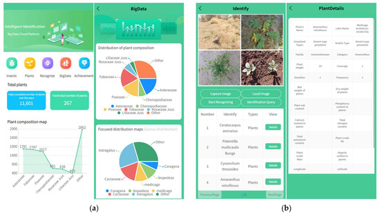
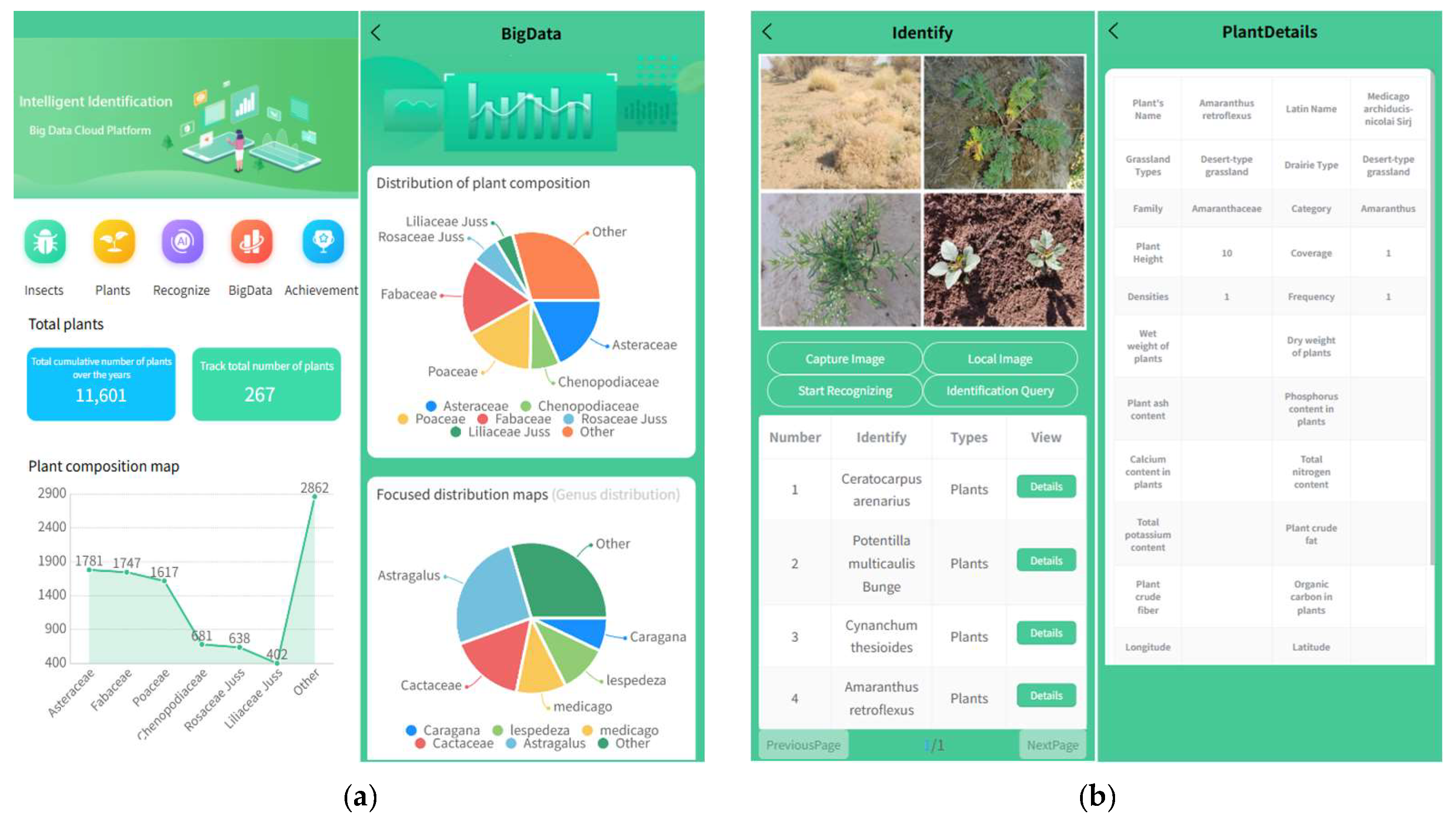
As illustrated in Figure 12, the desert grassland plant recognition system integrates a mobile client, a business management platform, and a backend plant recognition model to provide an efficient and reliable recognition service. The Flask server acts as the core of the business management platform, handling user requests, managing image data streams, and coordinating interactions between the mobile client and the recognition model. Upon receiving an image uploaded by the mobile client user, the server triggers image preprocessing through the PyTorch inference engine and forwards the processed data to the plant recognition model deployed on the cloud server. The model performs feature extraction, classification, and result generation, returning predicted plant species and associated confidence scores. This modular architecture ensures stable system operation, efficient request handling, and a smooth user experience. The user interface of each module in the mobile recognition app is shown in Figure 13.

Figure 13. Screenshots of the mobile application interface. (a) Real-time recognition interface showing species identification with confidence scores and ecological details; (b) data contribution interface allowing users to submit new plant images with optional manual verification.

As presented in Figure 13, the mobile application offers two core functions to support plant recognition and data collection in desert grassland scenarios. (a) Real-time Recognition: Users can either capture photos in real time or select images from their mobile device gallery. The images are uploaded to a cloud server, which invokes the deployed YOLOv11-PKD model for automatic species identification. Under a standard 4G mobile network, the system returns recognition results with an average latency of 1.05 s (based on 500 independent trials), delivering near-instantaneous feedback. The result interface displays the predicted species along with a confidence score and allows users to access detailed ecological information, including grassland type, vegetation coverage, plant height, density, and frequency. (b) Data Contribution: The mobile application also integrates a crowdsourcing mechanism, enabling users to submit captured images (accompanied by optional manual verification) to the central plant image database. This functionality facilitates the continuous expansion of the dataset, enhances the model’s recognition scope over time, and establishes valuable data resources for future scientific research on desert grasslands.

5. Conclusions

This study presents a lightweight plant recognition method for desert grasslands based on model pruning and knowledge distillation. The enhanced teacher model, YOLOv11-STC, incorporating the SPPCSPC module, Triplet Attention, and a Slim Neck structure, achieved an mAP50 of 88.3% on the DGPlant48 dataset. Through structured pruning (35% pruning rate) and L2 distillation, we derived the compact YOLOv11-PKD model, which retained an mAP50 of 87.9% while being only 5.0 MB in size, significantly outperforming other lightweight models. The proposed model was successfully deployed in a mobile application, enabling field identification with an average response time of approximately 1 s and serving as a practical tool for plant resource surveys in desert grassland ecosystems.

References

- Lu, J.; Feng, S.; Wang, S.; Zhang, B.; Ning, Z.; Wang, R.; Chen, X.; Yu, L.; Zhao, H.; Lan, D.; et al. Patterns and driving mechanism of soil organic carbon, nitrogen, and phosphorus stoichiometry across northern China’s desert-grassland transition zone. Catena 2023, 220, 106695. [Google Scholar] [CrossRef] [Scilit]
- Tian, R.; Zhang, J.; Feng, C.; Suo, M.; Zhang, Y.; Gao, X.; Zhao, Y.; Xu, Z. Effects of short-term restoration measures on community structure and biomass of desert steppe in dry and wet years. Acta Agrestia Sin. 2024, 32, 2106–2117. (In Chinese) [Google Scholar]
- Li, T.; Yin, J.; Zhong, K. Does financial support for grassland conservation and restoration improve ecological benefits? Evidence from China. Ecol. Indic. 2024, 159, 111628. [Google Scholar] [CrossRef] [Scilit]
- Steidl, R.J.; Litt, A.R.; Matter, W.J. Effects of plant invasions on wildlife in desert grasslands. Wildl. Soc. Bull. 2013, 37, 527–536. [Google Scholar] [CrossRef] [Scilit]
- Zhao, C.; Shao, M.A.; Jia, X.; Zhu, Y. Factors affecting soil desiccation spatial variability in the Loess Plateau of China. Soil Sci. Soc. Am. J. 2019, 83, 266–275. [Google Scholar] [CrossRef] [Scilit]
- Brookshire, E.N.J.; Weaver, T. Long-term decline in grassland productivity driven by increasing dryness. Nat. Commun. 2015, 6, 7148. [Google Scholar] [CrossRef] [Scilit] [PubMed]
- Lei, T.; Feng, J.; Lv, J.; Wang, J.; Song, H.; Song, W.; Gao, X. Net primary productivity loss under different drought levels in different grassland ecosystems. J. Environ. Manag. 2020, 274, 111144. [Google Scholar] [CrossRef] [Scilit] [PubMed]
- Du, Z.; Zhang, X.; Liu, S.; An, H. Nitrogen and water addition alters species diversity and interspecific relationship in a desert grassland. Sci. Total Environ. 2024, 908, 168386. [Google Scholar] [CrossRef] [Scilit]
- Voigt, W.; Perner, J.; Hefin Jones, T. Using functional groups to investigate community response to environmental changes: Two grassland case studies. Glob. Change Biol. 2007, 13, 1710–1721. [Google Scholar] [CrossRef] [Scilit]
- Xu, D.; Chen, B.; Shen, B.; Wang, X.; Yan, Y.; Xu, L.; Xin, X. The classification of grassland types based on object-based image analysis with multisource data. Rangel. Ecol. Manag. 2019, 72, 318–326. [Google Scholar] [CrossRef] [Scilit]
- Bardgett, R.D.; Bullock, J.M.; Lavorel, S.; Manning, P.; Schaffner, U.; Ostle, N.; Chomel, M.; Durigan, G.; LFry, E.; Johnson, D.; et al. Combatting global grassland degradation. Nat. Rev. Earth Environ. 2021, 2, 720–735. [Google Scholar] [CrossRef] [Scilit]
- Yang, Z.; He, W.; Fan, X.; Tjahjadi, T. PlantNet: Transfer learning-based fine-grained network for high-throughput plants recognition. Soft Comput. 2022, 26, 10581–10590. [Google Scholar] [CrossRef] [Scilit]
- Hasan, M.J.; Mazumdar, S.; Momen, S. Deployable deep learning for cross-domain plant leaf disease detection via ensemble learning, knowledge distillation, and quantization. IEEE Access. 2025, 13, 140313–140336. [Google Scholar] [CrossRef] [Scilit]
- Sankey, J.B.; Sankey, T.T.; Li, J.; Ravi, S.; Wang, G.; Caster, J.; Kasprak, A. Quantifying plant-soil-nutrient dynamics in rangelands: Fusion of UAV hyperspectral-LiDAR, UAV multispectral-photogrammetry, and ground-based LiDAR-digital photography in a shrub-encroached desert grassland. Remote Sens. Environ. 2021, 253, 112223. [Google Scholar] [CrossRef] [Scilit]
- LeCun, Y.; Bottou, L.; Bengio, Y.; Haffner, P. Gradient-based learning applied to document recognition. Proc. IEEE 1998, 86, 2278–2324. [Google Scholar] [CrossRef] [Scilit]
- Krizhevsky, A.; Sutskever, I.; Hinton, G.E. ImageNet classification with deep convolutional neural networks. Commun. ACM 2017, 60, 84–90. [Google Scholar] [CrossRef] [Scilit]
- Jeon, W.S.; Rhee, S.Y. Plant leaf recognition using a convolution neural network. Int. J. Fuzzy Log. Intell. Syst. 2017, 17, 26–34. [Google Scholar] [CrossRef] [Scilit]
- Mohamed, S.J.; Rihan, H.Z.; Aljafer, N.; Fuller, M.P. The impact of light spectrum and intensity on the growth, physiology, and antioxidant activity of lettuce (Lactuca sativa L.). Plants 2021, 10, 2162. [Google Scholar] [CrossRef] [Scilit]
- Gavrilescu, M. Water, soil, and plants interactions in a threatened environment. Water 2021, 13, 2746. [Google Scholar] [CrossRef] [Scilit]
- Dünser, B.; Möller, A.; Fondriest, V.; Boeckle, M.; Lampert, P.; Pany, P. Attitudes towards plants–exploring the role of plants’ ecosystem services. J. Biol. Educ. 2025, 59, 124–138. [Google Scholar] [CrossRef] [Scilit]
- Mendoza-Bernal, J.; Gonzalez-Vidal, A.; Skarmeta, A.F. A Convolutional Neural Network approach for image-based anomaly detection in smart agriculture. Expert Syst. Appl. 2024, 247, 123210. [Google Scholar] [CrossRef] [Scilit]
- Chen, Y.; Huang, Y.; Zhang, Z.; Wang, Z.; Liu, B.; Liu, C.; Huang, C.; Dong, S.; Pu, X.; Wan, F.; et al. Plant image recognition with deep learning: A review. Comput. Electron. Agric. 2023, 212, 108072. [Google Scholar] [CrossRef] [Scilit]
- Wu, H.; Fang, L.; Yu, Q.; Yang, C. Composite descriptor based on contour and appearance for plant species identification. Eng. Appl. Artif. Intell. 2024, 133, 108291. [Google Scholar] [CrossRef] [Scilit]
- Li, J.; Sun, S.; Jiang, H.; Tian, Y.; Xu, X. Image recognition and empirical application of desert plant species based on convolutional neural network. J. Arid Land 2022, 14, 1440–1455. [Google Scholar] [CrossRef] [Scilit]
- Fan, X.; Luo, P.; Mu, Y.; Zhou, R.; Tjahjadi, T.; Ren, Y. Leaf image based plant disease identification using transfer learning and feature fusion. Comput. Electron. Agric. 2022, 196, 106892. [Google Scholar] [CrossRef] [Scilit]
- Basavegowda, D.H.; Schleip, I.; Mosebach, P.; Weltzien, C. Deep learning-based detection of indicator species for monitoring biodiversity in semi-natural grasslands. Environ. Sci. Ecotechnol. 2024, 21, 100419. [Google Scholar] [CrossRef] [Scilit]
- Liang, Y.; Jiang, W.; Liu, Y.; Wu, Z.; Zheng, R. Picking-Point Localization Algorithm for Citrus Fruits Based on Improved YOLOv8 Model. Agriculture 2025, 15, 237. [Google Scholar] [CrossRef] [Scilit]
- Hu, Y.; Liu, G.; Chen, Z.; Liu, J.; Guo, J. Lightweight one-stage maize leaf disease detection model with knowledge distillation. Agriculture 2023, 13, 1664. [Google Scholar] [CrossRef] [Scilit]
- Wang, Y.P.; Li, Q.S.; Kizilbek, G.M.; Yan, S.; Liu, T.T.; Sun, W.; Cao, S.S. 2020–2021 image dataset for deep learning identification of desert plants in Xinjiang. Chin. Sci. Data 2023, 8, 264–270. (In Chinese) [Google Scholar]
- Wang, C.Y.; Bochkovskiy, A.; Liao, H.Y.M. YOLOv7: Trainable bag-of-freebies sets new state-of-the-art for real-time object detectors. In Proceedings of the IEEE/CVF Conference on Computer Vision and Pattern Recognition, Vancouver, BC, Canada, 18–22 June 2023; pp. 7464–7475. [Google Scholar]
- Misra, D.; Nalamada, T.; Arasanipalai, A.U.; Hou, Q. Rotate to attend: Convolutional triplet attention module. In Proceedings of the IEEE/CVF Winter Conference on Applications of Computer Vision, Waikoloa, HI, USA, 3–8 January 2021; pp. 3139–3148. [Google Scholar]
- Li, H.; Li, J.; Wei, H.; Liu, Z.; Zhan, Z.; Ren, Q. Slim-neck by GSConv: A lightweight-design for real-time detector architectures. J. Real-Time Image Process. 2024, 21, 62. [Google Scholar] [CrossRef] [Scilit]
- He, K.; Zhang, X.; Ren, S.; Sun, J. Spatial pyramid pooling in deep convolutional networks for visual recognition. IEEE Trans. Pattern Anal. Mach. Intell. 2015, 37, 1904–1916. [Google Scholar] [CrossRef] [Scilit]
- Wang, C.Y.; Liao, H.Y.M.; Wu, Y.H.; Chen, P.Y.; Hsieh, J.W.; Yeh, I.H. CSPNet: A new backbone that can enhance learning capability of CNN. In Proceedings of the IEEE/CVF Conference on Computer Vision and Pattern Recognition Workshops, Seattle, WA, USA, 13–19 June 2020; pp. 390–391. [Google Scholar]
- Li, W.; Xu, X.; Wang, W.; Chen, J. Lightweight Plant Disease Detection With Adaptive Multi-Scale Model and Relationship-Based Knowledge Distillation. Expert Syst. 2025, 42, e70059. [Google Scholar] [CrossRef] [Scilit]
- Han, S.; Pool, J.; Tran, J.; Dally, W. Learning both weights and connections for efficient neural network. In Proceedings of the Advances in Neural Information Processing Systems 28: Annual Conference on Neural Information Processing Systems 2015, Montreal, QC, Canada, 7–12 December 2015. [Google Scholar]
- Hinton, G.; Vinyals, O.; Dean, J. Distilling the knowledge in a neural network. arXiv 2015, arXiv:1503.02531. [Google Scholar] [CrossRef] [Scilit]
- Mengisti Berihu Girmay, S.O. Explainable AI: Leaf-based medicinal plant classification using knowledge distillation. In 44. GIL-Jahrestagung, Biodiversität Fördern Durch Digitale Landwirtschaft; Gesellschaft für Informatik e.V.: Bonn, Germany, 2024; pp. 23–34. [Google Scholar]
- Romero, A.; Ballas, N.; Kahou, S.E.; Chassang, A.; Gatta, C.; Bengio, Y. Fitnets: Hints for thin deep nets. arXiv 2014, arXiv:1412.6550. [Google Scholar]
- Zhao, B.; Cui, Q.; Song, R.; Qiu, Y.; Liang, J. Decoupled knowledge distillation. In Proceedings of the IEEE/CVF Conference on Computer Vision and Pattern Recognition, New Orleans, LA, USA, 18–24 June 2022; pp. 11953–11962. [Google Scholar]
- Zhao, N.; Tong, J. Optimized vegetable disease recognition model based on multi-dimensional attention and knowledge distillation strategy. Meas. Sci. Technol. 2025, 36, 075411. [Google Scholar] [CrossRef] [Scilit]
- Li, D.; Sun, J.; Liu, Y. Hierarchical semantic alignment heterogeneous knowledge distillation model for smart agriculture crop leaf disease recognition. Expert Syst. Appl. 2025, 296, 129100. [Google Scholar] [CrossRef] [Scilit]
- Howard, A.; Sandler, M.; Chu, G.; Chen, L.C.; Chen, B.; Tan, M.; Wang, W.; Zhu, Y.; Pang, R.; Vasudevan, V.; et al. Searching for mobilenetv3. In Proceedings of the IEEE/CVF International Conference on Computer Vision, Long Beach, CA, USA, 15–20 June 2019; pp. 1314–1324. [Google Scholar]
- Tan, M.; Le, Q. Efficientnet: Rethinking model scaling for convolutional neural networks. In Proceedings of the International Conference on Machine Learning, Long Beach, CA, USA, 9–15 June 2019; pp. 6105–6114. [Google Scholar]
- El Alaoui, A.; Mousannif, H. Enhancing weed detection through knowledge distillation and attention mechanism. Front. Robot. AI 2025, 12, 1654074. [Google Scholar] [CrossRef] [Scilit]
Disclaimer/Publisher’s Note: The statements, opinions and data contained in all publications are solely those of the individual author(s) and contributor(s) and not of MDPI and/or the editor(s). MDPI and/or the editor(s) disclaim responsibility for any injury to people or property resulting from any ideas, methods, instructions or products referred to in the content. |
© 2026 by the authors. Licensee MDPI, Basel, Switzerland. This article is an open access article distributed under the terms and conditions of the Creative Commons Attribution (CC BY) license.