Trajectory Tracking Control of an Orchard Mobile Robot Based on an Adaptive Super-Twisting Extended State Observer and Dynamic Power–Logarithmic Sliding Mode Control

Abstract

To address the degradation in drive-wheel speed control accuracy and vehicle trajectory-tracking performance caused by variations in wheel–terrain adhesion, load fluctuations, and model uncertainties under unstructured terrain conditions, a composite control method based on an adaptive super-twisting extended state observer and dynamic power-logarithmic sliding mode control is proposed. First, a kinematic model of a four-wheel differential-drive orchard mobile robot and a dynamic model of the drive motor incorporating lumped disturbances are established, and a dual closed-loop control system comprising a kinematic outer loop and a wheel-speed inner loop is constructed. Second, a super-twisting extended state observer with an adaptive gain adjustment mechanism is designed to estimate the drive-wheel angular acceleration and lumped disturbances online. Subsequently, a dynamic power-logarithmic sliding mode controller is developed, and the estimated disturbances are employed for feedforward compensation to improve wheel-speed response, disturbance-rejection performance, and control-input smoothness. Drive-system simulations, circular-trajectory simulations, and real-vehicle S-shaped trajectory-tracking experiments on natural turf are conducted to compare the proposed method with ESO–DCLSMC and DP–LnSMC. The results show that, in the drive-system simulations, the proposed method achieves a wheel-speed settling time of 50 ms and a maximum angular-velocity deviation of 0.009 rad·s⁻¹ under pulse load disturbances. In the real-vehicle experiments, the root-mean-square errors of position and heading angle are 10.51 cm and 0.050 rad, respectively, representing reductions of 29.78% and 24.70% compared with ESO–DCLSMC and 36.88% and 42.17% compared with DP–LnSMC, respectively. These results demonstrate that, under the natural grass terrain tested in this study, the proposed method achieves favorable trajectory-tracking accuracy and provides a feasible solution for trajectory-tracking control of orchard mobile robots operating under unstructured terrain conditions.

1. Introduction

With the rapid development of precision agriculture and intelligent agricultural production, orchard mobile robots have gradually become essential platforms for tasks such as environmental perception, crop protection, weed control, material transportation, and fruit harvesting [1,2,3]. Autonomous navigation is the foundation for enabling continuous and precision operations of orchard mobile robots, while trajectory tracking control, as a critical component of the autonomous navigation system, directly determines the robot’s operational accuracy, motion stability, and task execution efficiency [4]. At present, trajectory tracking control methods for agricultural mobile robots mainly include the Pure Pursuit algorithm [5], proportional–integral–derivative (PID) control [6], fuzzy control [7], model predictive control (MPC) [8], and sliding mode control (SMC) [9]. Owing to its fast dynamic response, relatively simple structure, and strong robustness against parameter perturbations and external disturbances, sliding mode control has been widely applied to trajectory tracking of intelligent agricultural machinery and wheeled mobile robots [10]. Li et al. developed an adaptive sliding mode path-tracking controller for an unmanned rice transplanter, in which the control parameters were adjusted online to improve tracking performance under uncertain operating conditions [11]. To mitigate trajectory errors and control chattering induced by uneven terrain, Luo et al. proposed a time-varying integral terminal sliding mode surface combined with a continuous switching function and an improved double-power reaching law, thereby accelerating the convergence of position and attitude errors while improving the smoothness of the control input for an orchard mobile robot [12]. Although these studies have significantly enhanced the trajectory tracking performance of agricultural mobile robots, conventional sliding mode control generally relies on high-gain switching terms to suppress unknown disturbances, which tends to introduce high-frequency oscillations in the control input and consequently increases the mechanical and electrical stresses imposed on motor drivers and transmission components [13]. Moreover, the trajectory tracking performance of four-wheel differential-drive orchard mobile robots depends not only on the outer-loop kinematic controller but also critically on the dynamic characteristics of the drive motors and the tracking accuracy of the inner-loop wheel speed controller. In practical orchard environments, where soil conditions, crop characteristics, and climatic factors vary considerably, the robot is inevitably subjected to severe modeling uncertainties and external disturbances [14]. To enhance the robustness of disturbed systems, the integrated design of disturbance observers and robust control strategies has attracted extensive attention. Lu et al. combined a nonlinear disturbance observer with model predictive control and sliding mode control to estimate and compensate for model uncertainties and external disturbances online, thereby improving the trajectory tracking performance of an autonomous tractor–trailer system [15]. Previous studies have demonstrated that disturbance observer-based control methods are highly effective in compensating for unknown external disturbances and model uncertainties in disturbed systems [16]. Therefore, the coordinated design of disturbance observation and robust control provides an effective approach for improving the adaptability of agricultural equipment operating under complex environmental conditions [17,18].

To address the above issues, this study extends the kinematic trajectory-tracking framework for orchard mobile robots presented in [12] by further considering drive-system dynamics, load variations under complex terrain conditions, and model uncertainties, thereby investigating the cascaded kinematic–drive-dynamic trajectory-tracking problem of a four-wheel differential-drive robot. Unlike [12], which primarily focused on position and orientation control at the kinematic level, the present study establishes a dynamic model of the four drive-wheel motors incorporating lumped disturbances and develops a dual-loop control architecture consisting of an outer-loop vehicle kinematic controller and an inner-loop drive-wheel speed controller. Building on adaptive super-twisting theory [19] and the ESO-based dual-loop control framework [20], an ASTESO is designed to estimate the drive-wheel states and lumped disturbances. Projection-constrained adaptive gain adjustment is introduced to balance the observer response during disturbance variations and noise suppression under steady-state conditions. For the inner wheel-speed loop, a dynamic power–logarithmic sliding surface is constructed, and IFPRRL [20] is adopted as the reaching law. Meanwhile, the disturbance estimates provided by the ASTESO are incorporated as feedforward compensation to improve the transient response, steady-state tracking accuracy, and control-input smoothness of the wheel-speed controller. Theoretical analysis establishes the finite-time convergence of the observation errors and the boundedness of the wheel-speed tracking errors in the presence of disturbance-estimation residuals. Finally, the tracking performance and practical implementability of the proposed control architecture are validated through drive-system simulations, full-vehicle trajectory-tracking simulations, and field experiments conducted on natural grass-covered terrain.

2. Materials and Methods

2.1. Experimental Platform for the Four-Wheel Differential-Drive Orchard Mobile Robot

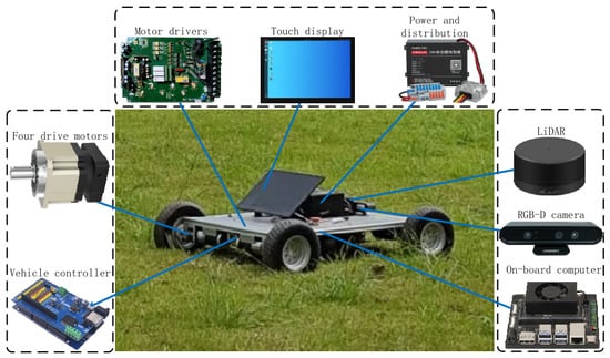
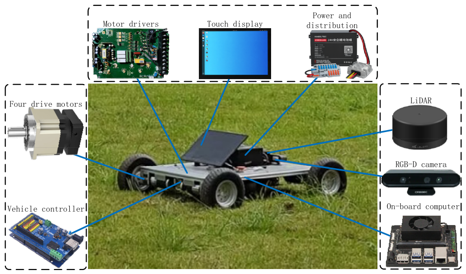
The trajectory tracking accuracy and operational stability of an orchard mobile robot are directly related to the quality of field operations and the reliability of its autonomous navigation system. To facilitate the rapid validation and performance evaluation of trajectory tracking control algorithms, an experimental platform based on a four-wheel differential-drive orchard mobile robot was developed in this study. The platform is designed for orchard environmental information acquisition, autonomous navigation, and trajectory tracking experiments. Its overall configuration and the main hardware components are illustrated in Figure 1.

Figure 1. Experimental platform and main hardware components of the four-wheel differential-drive orchard mobile robot.

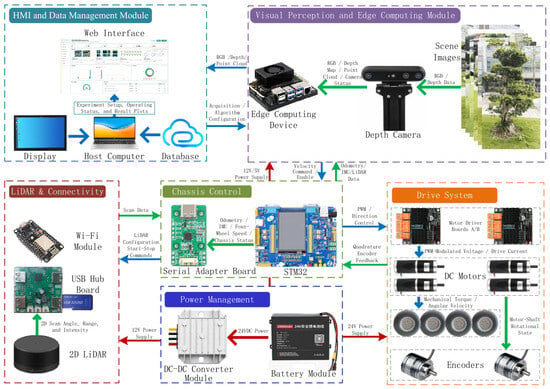
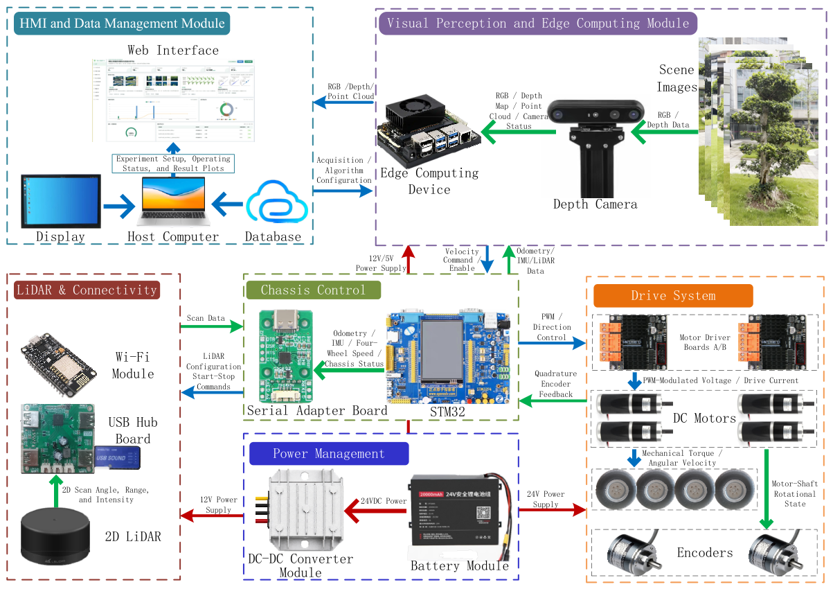
The experimental platform primarily consists of verified perception, computing, and low-level control hardware, including an Astra S RGB-D camera (Orbbec, Shenzhen, China), an M10P two-dimensional (2D) LiDAR (Leishen Intelligent System Co., Ltd., Shenzhen, China), an NVIDIA Jetson edge computing platform (NVIDIA Corporation, Santa Clara, CA, USA), and a chassis controller based on the STM32F407VET6 microcontroller (STMicroelectronics, Amsterdam, The Netherlands). The chassis, together with its associated low-level drive and control hardware, was sourced from the WHEELTEC mobile platform (WHEELTEC, Dongguan, China). Data communication between the Jetson edge computing platform and the chassis controller is implemented through a USB-UART serial communication interface based on the CH343 chip, which is supplied by Nanjing Qinheng Microelectronics Co., Ltd. (Nanjing, China). In addition, the experimental platform is equipped with a host monitoring computer and a display terminal for program deployment, parameter configuration, system status monitoring, and experimental data acquisition and storage. The hardware architecture and main technical specifications of the experimental platform are presented in Figure 2 and Table 1, respectively. Further details on the key hardware configuration and corresponding technical specifications are provided in Appendix A (Table A1).

Figure 2. Overall hardware architecture of the orchard mobile robot experimental platform.

Table 1. Main technical specifications of the orchard mobile robot experimental platform.

Parameter	Value
Overall dimensions (L × W × H)/mm	835 × 700 × 400
Total mass/kg	15.4
Maximum climbing angle/°	19
Maximum obstacle-crossing height/mm	75
Drive wheel diameter/mm	225
Maximum traveling speed/m·s−1	0.78
Maximum drive wheel angular velocity/rad·s−1	7.0162

The overall hardware architecture of the orchard mobile robot experimental platform is shown in Figure 2. The RGB-D depth camera is an Orbbec Astra S, which is connected to the NVIDIA Jetson Orin Nano 8 GB edge-computing platform via a USB interface for transmitting color images, depth images, and point-cloud data; the two-dimensional LiDAR is an LSLIDAR M10P, which is integrated into the system through a USB hub and a serial communication converter and transmits environmental scan data to the Jetson. A host computer communicates with the Jetson via a wireless network for algorithm configuration, operating-status monitoring, and experimental data management. The Jetson runs Ubuntu 20.04.6 and ROS 1 Noetic, performs perception-data processing and motion-command generation, and communicates with the WHEELTEC C50C/STM32F407VET6 main controller through a WCH CH343 USB-UART serial interface at a baud rate of 115,200 bit/s. It transmits vehicle linear-velocity, angular-velocity, and enable commands to the main controller while receiving vehicle motion-state information obtained from the low-level encoders and onboard IMU. The STM32 performs encoder data acquisition, low-level closed-loop wheel-speed control, and vehicle-velocity estimation, and packages the vehicle velocity, three-axis acceleration, three-axis angular velocity, and battery voltage into a 24-byte feedback frame for transmission to the Jetson; the ROS chassis node on the Jetson verifies the feedback frame, performs unit conversion, and publishes the data to generate wheel odometry, inertial measurements, and battery-voltage information. The average update frequency of the wheel odometry is approximately 20.001 Hz, while the trajectory controller operates at 30 Hz. According to the control commands, the STM32 outputs pulse-width modulation signals and direction-control signals, which are supplied to two WHEELTEC D50A dual-channel motor drivers to drive four MD60 P47 DC geared motors; the encoder on each drive wheel acquires the rotational state of the motor shaft in real time and feeds it back to the STM32, thereby forming the low-level closed-loop wheel-speed control system. The entire system is powered by a common 24 V traction battery, with the motor drivers supplied directly by the traction battery, while the different operating-voltage levels required by the sensors, controllers, and computing devices are converted and distributed through DC-DC converter modules.

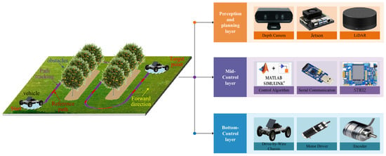
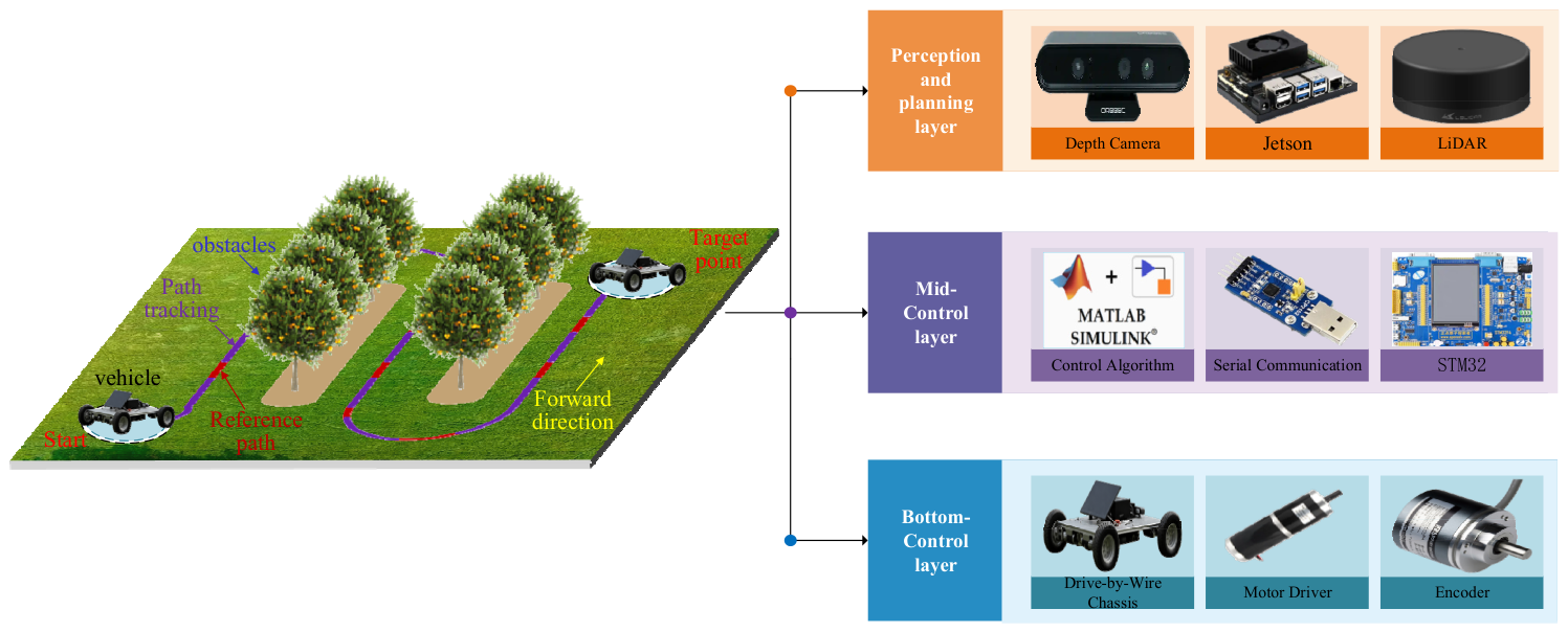
As shown in Figure 3, this study considers a typical operating scenario for an orchard mobile robot performing agricultural field operations. The robot tracks a predefined reference path by regulating the rotational speeds of the left and right wheel sets and the speed difference between them. The reference path consists of straight working segments and headland turning curves, forming a typical reciprocating inter-row operating route commonly used by agricultural machinery in field operations. By executing a headland turn, the robot can smoothly transition from the current working row to an adjacent crop row and subsequently continue the remaining field operations.

Figure 3. Typical Orchard Path-Tracking Scenario and Hierarchical Control Architecture.

According to the different requirements of the hardware components in terms of real-time performance and computational capability, the experimental platform is divided into three hierarchical layers: the perception and planning layer, the real-time control layer, and the execution layer.

(1)

Perception and planning layer. This layer mainly consists of a two-dimensional LiDAR sensor, an RGB-D depth camera, and the Jetson edge computing platform. The LiDAR and RGB-D camera are responsible for acquiring environmental ranging information, visual data, and depth information, respectively, while the Jetson platform performs sensor data processing, environmental perception, robot state estimation, and reference trajectory generation.

(2)

Real-time control layer. This layer consists of the trajectory tracking controller, the serial communication module, and the STM32 main controller. The trajectory tracking controller computes the desired linear velocity and angular velocity according to the current state of the orchard mobile robot and the reference trajectory. Based on the kinematic relationship of the four-wheel differential-drive system, the STM32 converts the vehicle velocity commands into the target angular velocities of the individual drive wheels and realizes closed-loop control of each drive wheel using encoder feedback.

(3)

Execution and drive layer. This layer comprises the motor drivers, DC motors, incremental encoders, and the four-wheel mobile chassis. The motor drivers actuate the DC motors according to the control signals generated by the STM32, while the encoders continuously measure the rotational speed of each drive wheel and feed the measurements back to the STM32. The orchard mobile robot achieves straight-line motion, steering, and continuous curved-path tracking through the differential motion of the left and right wheel sets.

2.2. Kinematic Modeling of the Orchard Mobile Robot

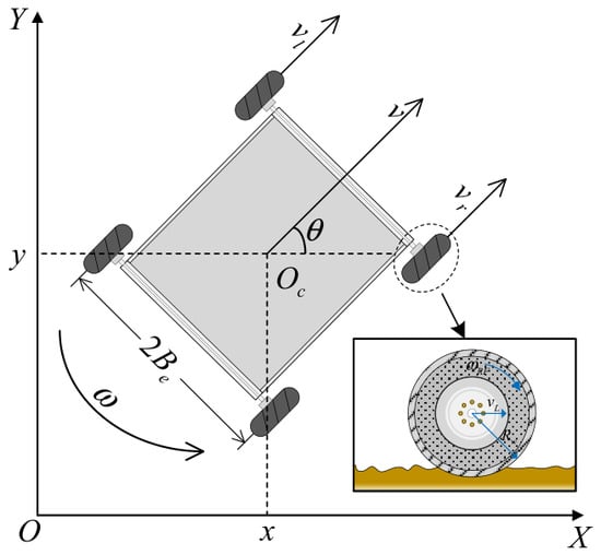
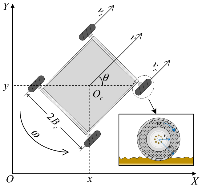
The research object of this study is a four-wheel differential-drive orchard mobile robot. The robot is driven by four independent DC motors, each actuating one wheel, while steering is achieved through the rotational speed difference between the left and right wheel sets. Since the robot primarily operates on a planar surface during inter-row orchard operations, the vehicle body is modeled as a rigid body. It is further assumed that the geometric center approximately coincides with the center of mass and that all four drive wheels maintain continuous and effective contact with the ground throughout operation. The kinematic configuration of the orchard mobile robot is illustrated in Figure 4.

Figure 4. Planar kinematic model of the orchard mobile robot. Note: XOY denotes the global coordinate frame, and O_c is the geometric center of the differential-drive chassis. x and y represent the coordinates of O_c in the global coordinate frame (m), and θ is the robot heading angle (rad). $\omega$ denotes the yaw angular velocity of the robot body (rad·s⁻¹). v_L and v_R are the equivalent linear velocities of the left and right wheel sets (m·s⁻¹), respectively. v is the actual traveling velocity of the robot (m·s⁻¹). $R_w$ denotes the effective rolling radius of the drive wheel (m). ${\omega }_{RF}$ is the actual angular velocity of the right front drive wheel (rad·s⁻¹), and $2B_e$ represents the effective track width of the robot (m).

Under the assumption that the lateral velocity at the geometric center of the vehicle body is approximately zero, the orchard mobile robot satisfies the following nonholonomic constraint:

$$-\dot{x}\sin \theta +\dot{y}\cos \theta =0$$

(1)

According to the planar rigid-body kinematics, the relationship between the pose and velocity of the orchard mobile robot can be expressed as:

$$\dot{\eta }=\left[\begin{array}{c}\dot{x}\\ \dot{y}\\ \dot{\theta }\end{array}\right]=\left[\begin{array}{cc}\cos \theta & 0\\ \sin \theta & 0\\ 0& 1\end{array}\right]\left[\begin{array}{c}v\\ \omega \end{array}\right].$$

(2)

Since the orchard mobile robot adopts a left–right differential-drive configuration, the front and rear wheels on the same side jointly form an equivalent drive wheel set during longitudinal motion. For a unified representation of the four drive wheels, the wheel set is defined as $W=\{LF,LR,RF,RR\}$, where LF, LR, RF, and RR denote the left-front, left-rear, right-front, and right-rear wheels, respectively. The corresponding angular velocities of the four drive wheels are denoted by ${\omega }_{LF}$, ${\omega }_{LR}$, ${\omega }_{RF}$, and ${\omega }_{RR}$.

Assuming that the effective rolling radius of all four drive wheels is $R_w$, the equivalent linear velocities of the left and right wheel sets are defined as the average of the angular velocities of the front and rear wheels on the corresponding side in order to reduce the influence of instantaneous wheel speed fluctuations, encoder measurement noise, and local wheel–ground contact variations on the vehicle kinematic computation:

$$\left\{\begin{array}{c}{v}_L={\displaystyle \frac{R_w}{2}}\left({\omega }_{LF}+{\omega }_{LR}\right),\hfill \\ v_R={\displaystyle \frac{R_w}{2}}\left({\omega }_{RF}+{\omega }_{RR}\right),\hfill \end{array}\right.$$

(3)

where $v_L$ and $v_R$ denote the equivalent linear velocities of the left and right drive wheel sets, respectively. The longitudinal linear velocity at the geometric center of the robot is determined by the average of the equivalent linear velocities of the left and right wheel sets, whereas the yaw angular velocity is determined by the difference between the equivalent linear velocities of the two wheel sets, which can be expressed as:

$$\left\{\begin{array}{c}v={\displaystyle \frac{v_L+v_R}{2}},\hfill \\ \omega ={\displaystyle \frac{v_R-v_L}{2B_e}},\hfill \end{array}\right.$$

(4)

where B_e denotes the effective half-track width, defined as the distance from the longitudinal centerline of the robot to the line of motion of the equivalent drive wheel set on either the left or right side. Within the specified low-speed operating range, B_e is regarded as a constant nominal parameter and is identified through constant-speed turning experiments, which can be expressed as: $B_e=(v_R-v_L)/2{\omega }_{\mathrm{imu}}$, where ${\omega }_{\mathrm{imu}}$ is the actual yaw angular velocity measured by the inertial measurement unit (IMU).

Substituting Equation (3) into Equation (4) yields the relationship between the vehicle body velocity and the angular velocities of the four drive wheels, which can be expressed as:

$$\left\{\begin{array}{c}v={\displaystyle \frac{R_w}{4}}\left({\omega }_{LF}+{\omega }_{LR}+{\omega }_{RF}+{\omega }_{RR}\right),\hfill \\ \omega ={\displaystyle \frac{R_w}{4B_e}}\left({\omega }_{RF}+{\omega }_{RR}-{\omega }_{LF}-{\omega }_{LR}\right).\hfill \end{array}\right.$$

(5)

Substituting Equation (5) into Equation (2) yields the state equations of the four-wheel differential-drive orchard mobile robot, which can be expressed as:

$$\left[\begin{array}{c}\dot{x}\\ \dot{y}\\ \dot{\theta }\end{array}\right]=\left[\begin{array}{cccc}{\displaystyle \frac{R_w\cos \theta }{4}}& {\displaystyle \frac{R_w\cos \theta }{4}}& {\displaystyle \frac{R_w\cos \theta }{4}}& {\displaystyle \frac{R_w\cos \theta }{4}}\\ {\displaystyle \frac{R_w\sin \theta }{4}}& {\displaystyle \frac{R_w\sin \theta }{4}}& {\displaystyle \frac{R_w\sin \theta }{4}}& {\displaystyle \frac{R_w\sin \theta }{4}}\\ -{\displaystyle \frac{R_w}{4B_e}}& -{\displaystyle \frac{R_w}{4B_e}}& {\displaystyle \frac{R_w}{4B_e}}& {\displaystyle \frac{R_w}{4B_e}}\end{array}\right]\left[\begin{array}{c}{\omega }_{LF}\\ {\omega }_{LR}\\ {\omega }_{RF}\\ {\omega }_{RR}\end{array}\right].$$

(6)

Equation (6) establishes the mapping between the global pose variation of the orchard mobile robot and the angular velocities of the four drive wheels. For given desired vehicle linear velocity $v_d$ and desired angular velocity ${\omega }_d$, an allocation strategy is adopted in which the desired angular velocities of the front and rear drive wheels on the same side are identical. The inverse kinematic solution can then be obtained from Equation (4), yielding the desired angular velocities of the four drive wheels, which can be expressed as:

$$\left\{\begin{array}{c}{\omega }_{LF,d}={\omega }_{LR,d}={\displaystyle \frac{v_d-B_e{\omega }_d}{R_w}}\hfill \\ {\omega }_{RF,d}={\omega }_{RR,d}={\displaystyle \frac{v_d+B_e{\omega }_d}{R_w}}\hfill \end{array}\right.$$

(7)

Equation (7) indicates that when the desired angular velocities of the left and right drive wheel sets are equal, the robot travels in a straight line along its current heading. When a speed difference exists between the two wheel sets, the robot undergoes the corresponding yaw motion, thereby achieving differential steering.

2.3. Dynamic Modeling of the Drive Wheel Motor System

Due to complex operating conditions in orchard inter-row environments, including soft soil, grass-covered ground, local terrain slopes, and variations in wheel–ground adhesion, the drive wheels are susceptible to rolling resistance, load disturbances, and unmodeled friction during operation. Therefore, it is necessary to establish the dynamic model relating the input voltage of the drive motor to the angular velocity of the drive wheel [21].

For the i-th drive wheel, where $i\in \mathcal{W}$, let ${\omega }_{m,i}$ denote the angular velocity of the drive motor output shaft, ${\omega }_i$ denote the corresponding angular velocity of the drive wheel, and $i_g$ denote the transmission ratio of the reduction gearbox. The relationship can be expressed as:

$${\omega }_{m,i}=i_g{\omega }_i$$

(8)

Let $K_{em}$ and $K_{tm}$ denote the back electromotive force (EMF) constant and the torque constant on the motor shaft side, respectively, and let ${\eta }_g$ denote the mechanical efficiency of the reduction gearbox and transmission mechanism. By referring the motor-side variables to the drive wheel side, the equivalent back EMF constant and equivalent torque constant can be obtained as:

$$K_e=i_g{K}_{em},K_t={\eta }_g{i}_g{K}_{tm}$$

(9)

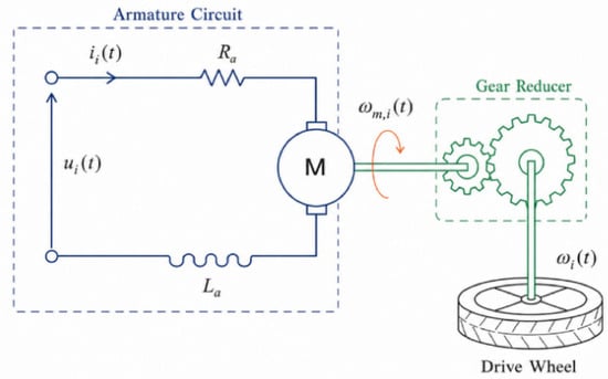
Based on the above parameter transformation, the equivalent circuit model of the i-th drive motor is illustrated in Figure 5.

Figure 5. Equivalent circuit model of a single-wheel DC drive unit.

According to the voltage balance equation of the DC motor armature circuit, while considering the equivalent rotational inertia, viscous damping, and external load torque referred to the drive wheel side, the electrical equation and the mechanical motion equation of the i-th drive unit can be expressed as:

$$\left\{\begin{array}{c}{u}_i=R_a{I}_i+L_a{\dot{I}}_i+K_e{\omega }_i\hfill \\ J_w{\dot{\omega }}_i+B_w{\omega }_i+T_{L,i}=K_t{I}_i\hfill \end{array}\right.$$

(10)

where $u_i$ is the equivalent input voltage of the motor, $R_a$ is the armature resistance, $L_a$ is the armature inductance, $I_i$ is the armature current, $J_w$ is the equivalent rotational inertia referred to the drive wheel side, $B_w$ is the viscous damping coefficient of the drive wheel, and $T_{L,i}$ is the external load torque acting on the i-th drive wheel, which mainly includes the rolling resistance torque, grade resistance torque, and disturbance torque caused by variations in wheel–ground adhesion conditions.

Eliminating the armature current $I_i$ from Equation (10) yields the second-order dynamic equation of the i-th drive unit, which can be expressed as:

$$L_a{J}_w{\ddot{\omega }}_i+\left(R_a{J}_w+L_a{B}_w\right){\dot{\omega }}_i+\left(R_a{B}_w+K_t{K}_e\right){\omega }_i=K_t{u}_i-R_a{T}_{L,i}-L_a{\dot{T}}_{L,i}$$

(11)

Under the assumptions of zero initial conditions and negligible external load torque, the transfer function between the input voltage and the angular velocity of the i-th drive wheel can be expressed as:

$$G_m(s)={\displaystyle \frac{{\Omega }_i(s)}{U_i(s)}}={\displaystyle \frac{K_t}{L_a{J}_w{s}^2+\left(R_a{J}_w+L_a{B}_w\right)s+R_a{B}_w+K_t{K}_e}},$$

(12)

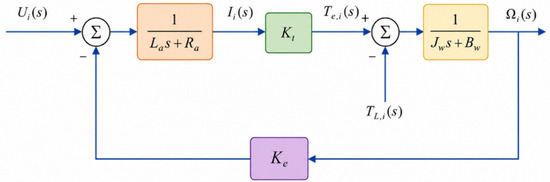
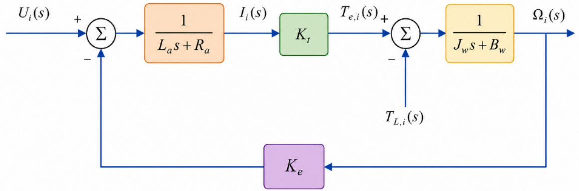
The corresponding dynamic block diagram is shown in Figure 6.

Figure 6. Dynamic block diagram of the single-wheel drive system.

For the design of the state observer and the wheel speed controller, Equation (11) is reformulated into the standard state-space representation, which can be expressed as:

$${\ddot{\omega }}_i=a_m{\dot{\omega }}_i+b_m{\omega }_i+c_m{u}_i+d_i(t),i\in W$$

(13)

where

$$a_m=-{\displaystyle \frac{R_a{J}_w+L_a{B}_w}{L_a{J}_w}},b_m=-{\displaystyle \frac{R_a{B}_w+K_t{K}_e}{L_a{J}_w}},c_m={\displaystyle \frac{K_t}{L_a{J}_w}}$$

(14)

In Equation (13), d_i(t) denotes the lumped disturbance acting on the i-th drive wheel and is defined as:

$$d_i(t)=-{\displaystyle \frac{R_a{T}_{L,i}+L_a{\dot{T}}_{L,i}}{L_a{J}_w}}+{\Delta }_i(t)$$

(15)

where ${\Delta }_i(t)$ represents the uncertainty caused by motor parameter perturbations, tire slip, variations in wheel–ground adhesion, and model simplification errors.

Furthermore, the state variables are defined as $x_{1i}={\omega }_i$ and $x_{2i}={\dot{\omega }}_i$. Accordingly, the state-space equation of the i-th drive wheel can be expressed as:

$$\left\{\begin{array}{c}{\dot{x}}_{1i}=x_{2i},\hfill \\ {\dot{x}}_{2i}=a_m{x}_{2i}+b_m{x}_{1i}+c_m{u}_i+d_i(t),\hfill \end{array}\right.i\in W.$$

(16)

where $x_{1i}$ and $x_{2i}$ denote the angular velocity of the drive wheel and its angular acceleration, respectively, $u_i$ is the control input, and $d_i(t)$ is an unknown but bounded lumped disturbance. In practical control applications, the physical limitations of the power supply and motor driver are taken into account, such that: $u_i\in \left[-U_{\max },U_{\max }\right]$.

2.4. Control System Design

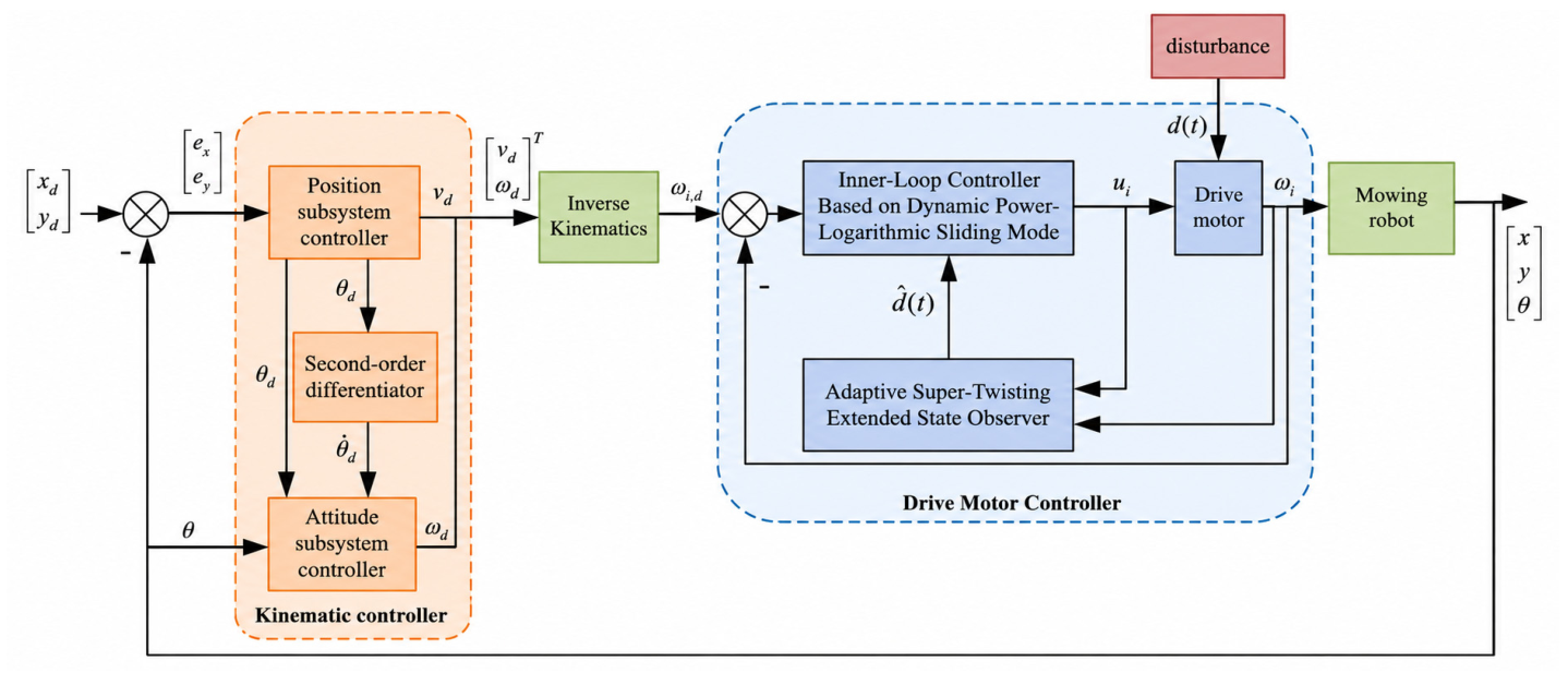
The orchard mobile robot exhibits nonholonomic constraints, strong coupling, and underactuated characteristics during inter-row field operations. To mitigate the adverse effects of complex terrain, wheel–ground contact uncertainty, and external disturbances on trajectory tracking performance, a dual-loop trajectory tracking control architecture is adopted in this study. The outer-loop controller generates the desired linear velocity and angular velocity commands based on the kinematic model of the orchard mobile robot, while the inner-loop controller achieves rapid tracking of the desired angular velocities of the four drive wheels based on the drive wheel dynamic model [22]. The overall architecture of the proposed control system is illustrated in Figure 7.

Figure 7. Dualloop trajectory tracking control structure of the orchard mobile robot.

2.4.1. Outer-Loop Kinematic Model Controller

According to Equation (2), the system has two independent control inputs and three state outputs, and therefore belongs to a nonholonomic underactuated system. Accordingly, the trajectory tracking problem is decomposed into a position subsystem and an attitude subsystem in this study. The position subsystem generates the desired heading angle ${\theta }_d$ and desired linear velocity $v_d$ based on the reference trajectory, while the attitude subsystem further generates the desired yaw angular velocity ${\omega }_d$ to ensure that the actual heading angle of the robot tracks ${\theta }_d$.

Let the desired trajectory be ${[x_d(t),y_d(t)]}^{\mathrm{T}}$, which is assumed to be twice continuously differentiable with bounded derivatives. The position tracking error is defined as:

$$e_x=x-x_d,e_y=y-y_d$$

(17)

According to the kinematic model of the orchard mobile robot, the position error dynamics can be derived as:

$$\left\{\begin{array}{c}{\dot{e}}_x=v\cos \theta -{\dot{x}}_d,\hfill \\ {\dot{e}}_y=v\sin \theta -{\dot{y}}_d.\hfill \end{array}\right.$$

(18)

To limit the magnitude of the velocity command caused by large initial tracking errors while ensuring that the virtual control input remains continuous and bounded, the virtual velocity components in the global coordinate frame are designed as:

$$\left\{\begin{array}{c}{u}_x={\dot{x}}_d-a_1\tanh (b_1{e}_x)\hfill \\ u_y={\dot{y}}_d-a_2\tanh (b_2{e}_y)\hfill \end{array}\right.$$

(19)

where $a_1,a_2,b_1,b_2>0$ are the position control parameters. Based on the virtual velocity components $u_x$ and $u_y$, the desired heading angle and the desired linear velocity can be determined as:

$${\theta }_d=\mathrm{atan}2(u_y,u_x),v_d=\sqrt{u_x^2+u_y^2}$$

(20)

Under the ideal attitude tracking condition, i.e., $\theta ={\theta }_d$ and $v=v_d$

$$v\cos \theta =u_x,v_d\sin {\theta }_d=u_y$$

(21)

Accordingly, the position error dynamics can be rewritten as:

$$\left\{\begin{array}{c}{\dot{e}}_x=-a_1\tanh (b_1{e}_x),\hfill \\ {\dot{e}}_y=-a_2\tanh (b_2{e}_y).\hfill \end{array}\right.$$

(22)

The Lyapunov function for the position subsystem is selected as:

$$V_p={\displaystyle \frac{1}{2}}{e}_x^2+{\displaystyle \frac{1}{2}}{e}_y^2.$$

(23)

Taking its time derivative yields:

$${\dot{V}}_p=-a_1{e}_x\tanh (b_1{e}_x)-a_2{e}_y\tanh (b_2{e}_y)\le 0.$$

(24)

For any $z\ne 0$ and $k>0$, the inequality $z\tanh (kz)>0$ always holds. Therefore, when $(e_x,e_y)\ne (0,0)$, ${\dot{V}}_p<0$. According to Lyapunov stability theory, under the ideal attitude tracking and velocity tracking conditions, the position tracking errors $e_x$ and $e_y$ asymptotically converge to zero.

Furthermore, the attitude tracking error is defined as $e_{\theta }=\theta -{\theta }_d$. To ensure that the actual heading angle rapidly and smoothly tracks the desired heading angle, the attitude subsystem control law is designed as:

$${\omega }_d={\dot{\theta }}_d-a_3\tanh (b_3{e}_{\theta })$$

(25)

where $a_3>0$ and $b_3>0$ are the control parameters of the attitude subsystem. Under the ideal angular velocity tracking condition, the attitude error dynamics can be expressed as:

$${\dot{e}}_{\theta }=\omega -{\dot{\theta }}_d=-a_3\tanh (b_3{e}_{\theta }).$$

(26)

The Lyapunov function for the attitude subsystem is selected as: $V_{\theta }=1/2e_{\theta }^2$. Taking its time derivative yields:

$${\dot{V}}_{\theta }=-a_3{e}_{\theta }\tanh (b_3{e}_{\theta })\le 0$$

(27)

Similarly, when $e_{\theta }\ne 0$, ${\dot{V}}_{\theta }<0$, indicating that the attitude tracking error $e_{\theta }$ asymptotically converges to zero. As the attitude tracking error gradually decreases, the actual velocity direction of the orchard mobile robot approaches the virtual velocity direction, thereby reducing the directional deviation in the position subsystem and ultimately achieving stable tracking of the desired trajectory.

Equation (25) requires the first-order derivative of the desired heading angle, ${\dot{\theta }}_d$. Since ${\theta }_d$ is computed using the arctangent function, obtaining its analytical derivative is relatively complicated and tends to amplify the high-frequency noise contained in the discretized reference trajectory and state measurements. Therefore, a linear second-order differentiator is employed to obtain a smooth estimate of ${\theta }_d$:

$$\left\{\begin{array}{c}{\dot{z}}_{1\theta }=z_{2\theta },\hfill \\ {\dot{z}}_{2\theta }=-r_{\theta }^2\left(z_{1\theta }-{\theta }_d\right)-2r_{\theta }{z}_{2\theta },\hfill \end{array}\right.$$

(28)

where $z_{1\theta }$ is the tracking estimate of the desired heading angle ${\theta }_d$, $z_{2\theta }$ is the estimate of its first-order derivative ${\dot{\theta }}_d$, and $r_{\theta }>0$ is the bandwidth parameter of the differentiator. Finally, the outer-loop controller generates the desired linear velocity $v_d$ and desired angular velocity ${\omega }_d$, which are used as the reference inputs for the inner-loop drive wheel speed controller.

2.4.2. Adaptive Super-Twisting Extended State Observer

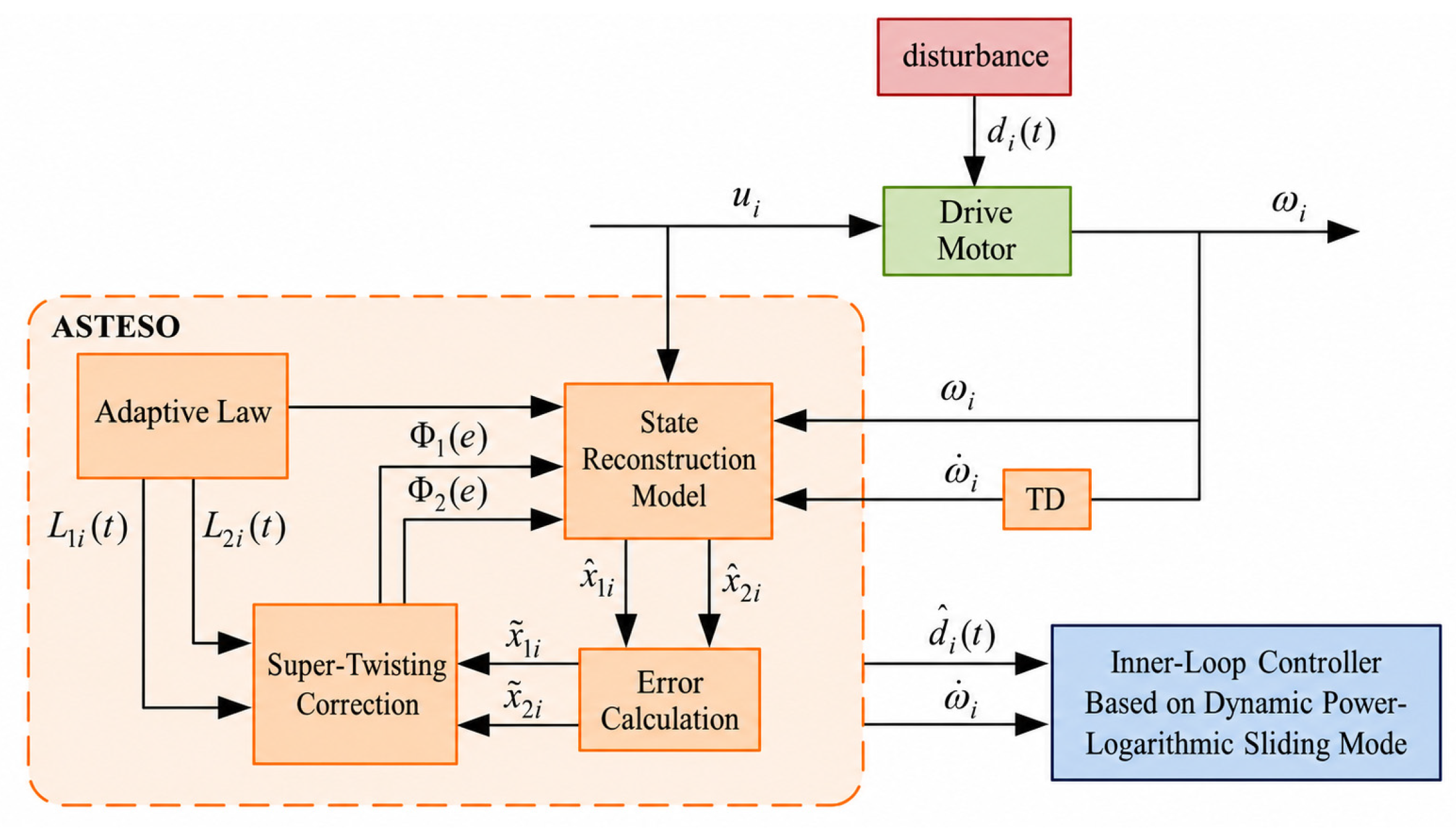
During inter-row operations, the orchard mobile robot is inevitably subjected to uncertainties such as variations in soil adhesion conditions, tire slip, uneven terrain, and unmodeled friction, which degrade the tracking accuracy of the drive wheel speed inner loop. To achieve online estimation of the drive system states and lumped disturbances [23], an adaptive super-twisting extended state observer (ASTESO) is proposed in this study. The overall structure of the observer is illustrated in Figure 8. By introducing a projection-based adaptive law to adjust the observer gains online, the proposed observer enhances the transient response during abrupt disturbance variations while simultaneously improving the suppression of measurement noise under steady-state conditions.

Figure 8. Block diagram of the adaptive super-twisting extended state observer.

Based on the dynamic model of the single-wheel drive system described by Equation (16), the state variables are defined as $x_{1i}={\omega }_i$, $x_{2i}={\dot{\omega }}_i$, and $x_{3i}=d_i(t)$. Accordingly, the i-th drive wheel motor system can be augmented into the following third-order system:

$$\left\{\begin{array}{cc}{\dot{x}}_{1i}=x_{2i},\hfill & \\ {\dot{x}}_{2i}=a_m{x}_{2i}+b_m{x}_{1i}+c_m{u}_i+x_{3i},\hfill & i\in W\hfill \\ {\dot{x}}_{3i}=h_i(t),\hfill & \end{array}\right.$$

(29)

where $h_i(t)$ denotes the rate of change of the lumped disturbance.

Assumption 1.

Within the normal low-speed operating range of the orchard mobile robot, the lumped disturbance $d_i(t)$is continuously differentiable. Moreover, there exist positive constants  ${\overline{d}}_i>0$ and ${\overline{h}}_i>0$ such that $|d_i(t)|\le {\overline{d}}_i$ and $|h_i(t)|\le {\overline{h}}_i$. In addition, the system states and the control input remain bounded within the prescribed operating region.

Let ${\widehat{x}}_{1i}$, ${\widehat{x}}_{2i}$, and ${\widehat{x}}_{3i}$ denote the estimates of $x_{1i}$, $x_{2i}$, and $x_{3i}$, respectively. The observation error is defined as ${\tilde{x}}_{ji}=x_{ji}-{\widehat{x}}_{ji}$, $j=1,2,3$. For the system described by Equation (29), the ASTESO is designed as:

$$\left\{\begin{array}{cc}{\dot{\widehat{x}}}_{1i}={\widehat{x}}_{2i}+k_0{\Phi }_1({\tilde{x}}_{1i}),\hfill & \\ {\dot{\widehat{x}}}_{2i}=a_m{\widehat{x}}_{2i}+b_m{x}_{1i}+c_m{u}_i+{\widehat{x}}_{3i}+L_{1i}(t){\Phi }_1({\tilde{x}}_{2i}),\hfill & i\in W\hfill \\ {\dot{\widehat{x}}}_{3i}=L_{2i}(t){\Phi }_2({\tilde{x}}_{2i}),\hfill & \end{array}\right.$$

(30)

where $k_0>0$ is the state reconstruction gain, $L_{1i}(t)$ and $L_{2i}(t)$ are the adaptive super-twisting gains, and the disturbance estimate is given by ${\widehat{d}}_i(t)={\widehat{x}}_{3i}(t)$.

To simultaneously achieve finite-time convergence and enhance the correction capability under large observation errors, the super-twisting nonlinear function is defined as:

$$\left\{\begin{array}{c}{\Phi }_1(e)=|e{|}^{1/2}\mathrm{sgn}(e)+e,\hfill \\ {\Phi }_2(e)={\Phi }_1^{\prime }(e){\Phi }_1(e)={\displaystyle \frac{1}{2}}\mathrm{sgn}(e)+{\displaystyle \frac{3}{2}}|e{|}^{1/2}\mathrm{sgn}(e)+e.\hfill \end{array}\right.$$

(31)

where, for $e\ne 0$, ${\Phi }_1^{\prime }(e)=1+{\displaystyle \frac{1}{2|e{|}^{1/2}}}>0$. The fractional-power term endows the observer with a non-Lipschitz characteristic in the vicinity of the origin, thereby providing the condition for finite-time convergence, while the linear term enhances the correction capability during the large-error transient stage.

To mitigate the amplification of measurement noise caused by fixed high observer gains while improving the observer’s responsiveness to abrupt load variations, the following projection-based adaptive gain law is designed:

$$\left\{\begin{array}{c}{\dot{L}}_{1i}={\mathrm{Proj}}_{[L_m,L_M]}\left(L_{1i},{\overline{\omega }}_i\right),\hfill \\ {\overline{\omega }}_i=\left\{\begin{array}{cc}{\gamma }_1\sqrt{{\displaystyle \frac{{\mathcal{l}}_1}{2}}}\mathrm{sgn}\left(\left|{\tilde{x}}_{2i}\right|-\mu \right),\hfill & L_{1i}>L_m,\hfill \\ \eta ,\hfill & L_{1i}\le L_m,\hfill \end{array}\right.\hfill \\ L_{2i}=2\epsilon L_{1i},\hfill \end{array}\right.$$

(32)

where $0<L_m<L_M$ denote the lower and upper bounds of the adaptive gain, respectively, ${\gamma }_1>0$, $\eta >0$, and $\epsilon >0$ are parameters of the adaptation law, and $\mu \ge 0$ denotes the width of the error dead zone. The projection operator constrains the adaptive gain such that $L_m\le L_{i1}(t)\le L_M$. When $\left|{\tilde{x}}_{2i}\right|>\mu$, $L_{1i}$ increases to improve the observer response to load variations; when $\left|{\tilde{x}}_{2i}\right|<\mu$, the gain gradually decreases, thereby suppressing the amplification of measurement noise. The projection operator guarantees $L_m\le L_{i1}(t)\le L_M$ ensuring that the gain continues to satisfy the finite-time stability condition of the super-twisting error subsystem during the gain-decreasing process. When $\mu =0$, the adaptation law reduces to a dead-zone-free form. Finite-time convergence is guaranteed by the relationship between the projected lower bound $L_m$ and the theoretical threshold $L_{1i}^{\ast }$.

According to the observation-error definitions given above, the observation-error dynamics shown in Equation (33) can be obtained, where ${\Phi }_1(\cdot )$ and ${\Phi }_2(\cdot )$ are the super-twisting nonlinear functions defined in Equation (31), respectively.

$$\left\{\begin{array}{c}{\dot{\tilde{x}}}_{1i}={\tilde{x}}_{2i}-k_0{\Phi }_1({\tilde{x}}_{1i}),\hfill \\ {\dot{\tilde{x}}}_{2i}=a_m{\tilde{x}}_{2i}+{\tilde{x}}_{3i}-L_{1i}{\Phi }_1({\tilde{x}}_{2i}),\hfill \\ {\dot{\tilde{x}}}_{3i}=h_i(t)-L_{2i}{\Phi }_2({\tilde{x}}_{2i}).\hfill \end{array}\right.$$

(33)

The last two equations in Equation (33) constitute the super-twisting error subsystem.

Theorem 1.

Consider the extended system in Equation (29) and the ASTESO in Equation (30). Suppose that Assumption 1 holds. Let $\mu \ge 0$, and assume that the initial observer gain satisfies $L_{1i}(0)\in [L_m,L_M]$. If the lower projection bound satisfies $L_m>\underset{i\in W}{max}{L}_{1i}^{\ast }$ then the observation errors and converge to zero in finite time in the Filippov sense [19].

Proof. 

For ${\tilde{x}}_{2i}\ne 0$, define the transformed variables as:

$${\zeta }_i=\left[\begin{array}{c}{\zeta }_{1i}\\ {\zeta }_{2i}\end{array}\right]=\left[\begin{array}{c}{\Phi }_1({\tilde{x}}_{2i})\\ {\tilde{x}}_{3i}\end{array}\right],{\alpha }_i={\displaystyle \frac{{\alpha }_m{\tilde{x}}_{2i}}{{\Phi }_1({\tilde{x}}_{2i})}},{\beta }_i={\displaystyle \frac{h_i(t)}{{\Phi }_2({\tilde{x}}_{2i})}}.$$

(34)

$${\dot{\zeta }}_i={\Phi }_{1^{\prime }}({\tilde{x}}_{2i})A_i(t){\zeta }_i,A_i(t)=\left[\begin{array}{cc}-(L_{1i}-{\alpha }_i)& 1\\ -(2\epsilon L_{1i}-{\beta }_i)& 0\end{array}\right].$$

(35)

According to Equation (31) and Assumption 1, it follows that $\left|{\alpha }_i\right|\le \left|a_m\right|$ and $\left|{\beta }_i\right|\le 2{\overline{h}}_i$. The following Lyapunov function is selected:

$$\left\{\begin{array}{c}{V}_i={\zeta }_i^{\mathrm{T}}P{\zeta }_i,P=\left[\begin{array}{cc}\mathsf{\vartheta }+4{\epsilon }^2& -2\epsilon \\ -2\epsilon & 1\end{array}\right],\mathsf{\vartheta }>0,\hfill \\ {\dot{V}}_i=-{\Phi }_{1^{\prime }}({\tilde{x}}_{2i}){\zeta }_i^{\mathrm{T}}{Q}_i{\zeta }_i,Q_i=-\left(A_i^{\mathrm{T}}P+P{A}_i\right).\hfill \end{array}\right.$$

(36)

Since $\det (P_i)=\mathsf{\vartheta }>0$, the matrix $P_i$ is positive definite. According to the Schur complement condition, together with

$$L_{1i}>L_i^{\ast }=\max \left\{{\displaystyle \frac{(\mathsf{\vartheta }+4{\epsilon }^2)\left|a_m\right|+4\epsilon {\overline{h}}_i}{\mathsf{\vartheta }}}+{\displaystyle \frac{{\left(\mathsf{\vartheta }+4{\epsilon }^2+2\epsilon \left|a_m\right|+2{\overline{h}}_i\right)}^2}{8\epsilon \mathsf{\vartheta }}},{\displaystyle \frac{{\overline{h}}_i}{\epsilon }}\right\}$$

(37)

where $Q_i\succ 0$, the set-valued injection term in Equation (36) compensates for the bounded disturbance variation rate $h_i(t)$ at the error equilibrium, thereby preserving the invariance of the equilibrium set.

According to the projection mechanism in Equation (32), for any $t\ge 0$, it holds that $L_{1i}(t)\ge L_m>\underset{i\in W}{max}{L}_i^{\ast }$. Therefore, the sufficient condition given in Equation (37) is satisfied throughout the entire observation process, and the matrix $Q_i$ is uniformly positive definite. Hence, there exists a constant $q_i=in{f}_{t\ge 0}{\lambda }_{min}(Q_i(t))>0$ such that $Q_i\ge q_{i}I$. Combining ${\Phi }_1^{\prime }({\tilde{x}}_{2i})\ge 1/2\Vert {\zeta }_i\Vert$ with $V_i\le {\lambda }_{\max }(P_i)\Vert {\zeta }_i{\Vert }^2$ yields:

$${\dot{V}}_i\le -r_i{V}_i^{1/2},T_{23,i}\le {\displaystyle \frac{2V_i^{1/2}(0)}{r_i}},r_i={\displaystyle \frac{q_i}{2\sqrt{{\lambda }_{\max }(P)}}}>0$$

(38)

According to finite-time stability theory, ${\tilde{x}}_{2i}$ and ${\tilde{x}}_{3i}$ converge to zero within a finite time $T_{23,i}$. Therefore, when $t\ge T_{23,i}$, ${\tilde{x}}_{2i}={\tilde{x}}_{3i}=0$. At this stage, the first equation of the error system in Equation (33) degenerates into a scalar system involving only ${\tilde{x}}_{1i}$, yielding

$$\left\{\begin{array}{l}{D}^{+}\left|{\tilde{x}}_{1i}\right|=-k_0\left(|{\tilde{x}}_{1i}{|}^{1/2}+|{\tilde{x}}_{1i}|\right)\le -k_0|{\tilde{x}}_{1i}{|}^{1/2}\\ T_{o,i}\le T_{23,i}+{\displaystyle \frac{2{\left|{\tilde{x}}_{1i}\left(T_{23,i}\right)\right|}^{1/2}}{k_0}}\end{array}\right.$$

(39)

Hence, the observation errors ${\tilde{x}}_{1i}$, ${\tilde{x}}_{2i}$, and ${\tilde{x}}_{3i}$ all converge to zero within a finite time $T_{o,i}$, which completes the proof. The estimated drive wheel angular acceleration ${\tilde{x}}_{2i}$ and the lumped disturbance estimate ${\widehat{d}}_i={\widehat{x}}_{i3}$ provided by the observer are subsequently utilized in the wheel speed controller to compensate for load variations caused by orchard terrain and model uncertainties. □

2.4.3. Inner-Loop Drive Wheel Angular Velocity Controller Based on Dynamic Power–Logarithmic Sliding Mode Control

The outer-loop kinematic controller generates the desired linear velocity $v_d$ and desired angular velocity ${\omega }_d$, from which the desired angular velocities of the four drive wheels are obtained according to Equation (7). Based on the drive wheel dynamic model, a dynamic power–logarithmic sliding mode controller is designed in this study. The proposed controller employs the lumped disturbance estimate provided by the ASTESO for feedforward compensation and incorporates an improved fast power-rate reaching law to simultaneously achieve rapid transient response, high steady-state tracking accuracy, and smooth control input.

According to Equation (16), the angular velocity tracking error of the i-th drive wheel and its first- and second-order derivatives are defined as:

$$\left\{\begin{array}{cc}{e}_i={\omega }_{i,d}-{\omega }_i,\hfill & \\ {\dot{e}}_i={\dot{\omega }}_{i,d}-{\dot{\omega }}_i,\hfill & i\in W\hfill \\ {\ddot{e}}_i={\ddot{\omega }}_{i,d}-a_m{\dot{\omega }}_i-b_m{\omega }_i-c_m{u}_i-d_i(t),\hfill & \end{array}\right.$$

(40)

where ${\omega }_{i,d}$, ${\dot{\omega }}_{i,d}$, and ${\ddot{\omega }}_{i,d}$ denote the desired angular velocity of the i-th drive wheel and its first- and second-order derivatives, respectively.

To analyze the convergence characteristics of different sliding surfaces, the conventional linear sliding surface [24], terminal sliding surface [25], and nonsingular terminal sliding surface [26] are respectively expressed as:

$$\mathrm{LSMC}:s_i=c_{si}{e}_i+{\lambda }_i{\dot{e}}_i$$

(41)

$$\mathrm{TSMC}:s_i=c_{si}{e}_i^{q/p}+{\lambda }_i{\dot{e}}_i$$

(42)

$$\mathrm{NTSMC}:s_i=c_{si}{e}_i+{\lambda }_i{\dot{e}}_i^{q/p}$$

(43)

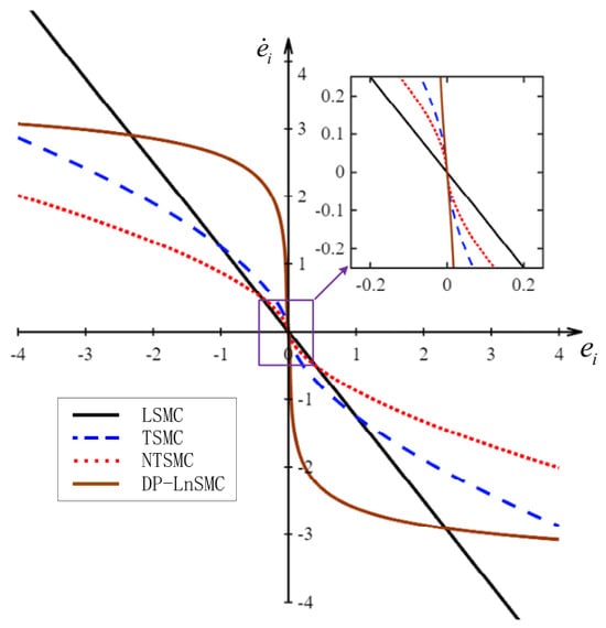
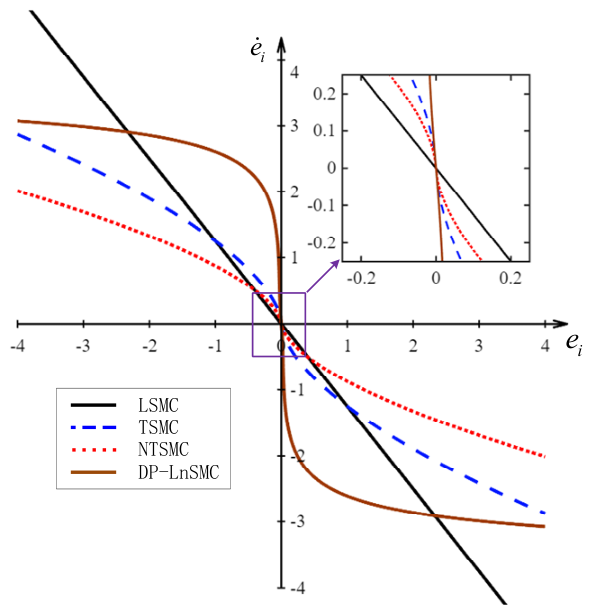
where $c_{si}>0$, ${\lambda }_i>0$, $p>q>0$, and $0<q/p<1$. The linear sliding surface has a simple structure but exhibits a limited convergence rate under large tracking errors. The terminal sliding surface achieves finite-time convergence; however, its control law may suffer from singularity. Although the nonsingular terminal sliding surface avoids this issue to some extent, its fractional-power structure may still cause excessive variations in the control input. To simultaneously achieve rapid convergence under large tracking errors and high steady-state accuracy under small tracking errors, a dynamic power–logarithmic sliding mode surface (DP-LnSMC) is proposed in this study:

$$s_i=c_{si}\ln \left(1+k_{si}\left|e_i\right|\right)\mathrm{sgn}(e_i)+{\lambda }_i{p}_i({\dot{e}}_i),$$

(44)

where $k_{si}>0$ is the tuning parameter of the logarithmic error term, and $p_i({\dot{e}}_i)$ is the nonsingular dynamic power function.

To ensure that the dynamic power function is continuously differentiable in the vicinity of the origin while preventing singularities caused by the denominator of the control law, $p_i({\dot{e}}_i)$ is defined as:

$$p_i({\dot{e}}_i)=\left\{\begin{array}{cc}|{\dot{e}}_i{|}^{{\displaystyle \frac{{\alpha }_{1i}|{\dot{e}}_i{|}^2}{1+{\alpha }_{2i}|{\dot{e}}_i{|}^2}}}\mathrm{sgn}({\dot{e}}_i),\hfill & \left|{\dot{e}}_i\right|\ge {\delta }_{1i},\hfill \\ {\delta }_{2i}{\dot{e}}_i\left({\delta }_{3i}-\left|{\dot{e}}_i\right|\right),\hfill & \left|{\dot{e}}_i\right|<{\delta }_{1i},\hfill \end{array}\right.$$

(45)

where ${\alpha }_{1i}>0$, ${\alpha }_{2i}>0$, and $0<{\delta }_{1i}<1$. The parameters ${\delta }_{2i}$ and ${\delta }_{3i}$ are determined according to the continuity conditions of $p_i({\dot{e}}_i)$ and its first-order derivative at $\left|{\dot{e}}_i\right|={\delta }_{1i}$. Let the function value and derivative of the outer-segment function at $r={\delta }_{1i}$ be denoted by $F_i({\delta }_{1i})$ and $F_i^{\prime }({\delta }_{1i})$, respectively. Then:

$${\delta }_{2i}={\displaystyle \frac{F_i({\delta }_{1i})-{\delta }_{1i}{F}_{i^{\prime }}({\delta }_{1i})}{{\delta }_{1i}^2}},{\delta }_{3i}=2{\delta }_{1i}+{\displaystyle \frac{F_{i^{\prime }}({\delta }_{1i})}{{\delta }_{2i}}}.$$

(46)

If the parameters satisfy $F_i^{\prime }({\delta }_{1i})>0$, and $F_i({\delta }_{1i})-{\delta }_{1i}{F}_i^{\prime }({\delta }_{1i})>0$, it follows that ${\delta }_{2i}>0$, ${\delta }_{3i}>2{\delta }_{1i}$. Consequently, $p_i({\dot{e}}_i)$ is a continuously differentiable odd function that remains monotonically increasing over the prescribed operating interval, thereby ensuring that $p_i({\dot{e}}_i)$ is bounded and nonzero.

Figure 9 illustrates the sliding trajectories of different sliding mode surfaces in the system error state plane. The introduction of the parameter $k_{si}$ provides DP-LnSMC with greater flexibility in adjusting the reaching time compared with LSMC and NTSMC. Furthermore, DP-LnSMC requires significantly fewer tuning parameters than TSMC and NTSMC, thereby improving its portability and facilitating controller deployment across different platforms. Increasing the value of $k_{si}$ can significantly shorten the reaching time. In regions far from the equilibrium point, the slope of the sliding mode surface gradually decreases, which helps reduce the initial control effort and mitigate the risk of actuator saturation, thereby enhancing the disturbance rejection capability of the control system.

Figure 9. Trajectories of different sliding mode surfaces in the error state plane.

Based on the proposed dynamic power-logarithmic sliding mode surface, differentiating Equation (44) yields:

$${\dot{s}}_i=A_i\left(e_i\right){\dot{e}}_i+B_i\left({\dot{e}}_i\right){\ddot{e}}_i$$

(47)

where

$$A_i\left(e_i\right)={\displaystyle \frac{c_{si}{k}_{si}}{1+k_{si}\left|e_i\right|}},B_i({\dot{e}}_i)={\lambda }_i{p}_i^{\prime }({\dot{e}}_i)>0$$

(48)

Substituting the error dynamics in Equation (40) into Equation (47) gives:

$${\dot{s}}_i=A_i(e_i){\dot{e}}_i+B_i({\dot{e}}_i)\left[{\ddot{\omega }}_{i,d}-a_m{\dot{\omega }}_i-b_m{\omega }_i-c_m{u}_i-d_i(t)\right]$$

(49)

To alleviate the trade-off between convergence speed and chattering suppression inherent in the conventional constant-rate and exponential reaching laws, an improved fast power rate reaching law (IFPRRL) is adopted:

$${\dot{s}}_i=-{\displaystyle \frac{k_{ri}}{{\rho }_i+{\sigma }_i^{\left|s_i\right|}}}{\left|s_i\right|}^{{\alpha }_i}\mathrm{sgn}\left(s_i\right)-{\displaystyle \frac{{\epsilon }_{ri}}{{\rho }_i+{\sigma }_i^{\left|s_i\right|}}}{s}_i$$

(50)

where $k_{ri}>0$, ${\epsilon }_{ri}>0$, ${\rho }_i>0$, $0<{\sigma }_i<1$, and $0<{\alpha }_i<1$ are the reaching law parameters. Define:

$$R_i(s_i)={\displaystyle \frac{k_{ri}}{{\rho }_i+{\sigma }_i^{|s_i|}}}|s_i{|}^{{\alpha }_i}\mathrm{sgn}(s_i)+{\displaystyle \frac{{\epsilon }_{ri}}{{\rho }_i+{\sigma }_i^{\left|s_i\right|}}}{s}_i$$

(51)

Combining Equations (49) and (51), and employing the disturbance estimate ${\widehat{d}}_i\left(t\right)$ provided by the ASTESO, the inner-loop control law for the i-th driving wheel can be derived as:

$$u_i={\displaystyle \frac{B_i({\dot{e}}_i)\left[{\ddot{\omega }}_{i,d}-a_m{\dot{\omega }}_i-b_m{\omega }_i-{\widehat{d}}_i(t)\right]+A_i(e_i){\dot{e}}_i+R_i(s_i)}{B_i({\dot{e}}_i)c_m}}.$$

(52)

Substituting Equation (52) into Equation (49) yields the closed-loop dynamics of the sliding variable:

$${\dot{s}}_i=-R_i(s_i)+B_i({\dot{e}}_i)\left[{\widehat{d}}_i(t)-d_i(t)\right]$$

(53)

It follows from Equation (53) that the reaching performance of the sliding variable is jointly determined by the reaching term and the disturbance-estimation residual. First, consider the nominal case in which the disturbance-estimation residual is zero, i.e., ${\widehat{d}}_i(t)=d_i(t)$. To analyze the stability of the sliding-mode reaching phase, the Lyapunov function is selected as $V_{si}=1/2s_i^2$, which yields:

$${\dot{V}}_{si}=s_i{\dot{s}}_i=-{\displaystyle \frac{k_{ri}}{{\rho }_i+{\sigma }_i^{\left|s_i\right|}}}{\left|s_i\right|}^{{\alpha }_i+1}-{\displaystyle \frac{{\epsilon }_{ri}}{{\rho }_i+{\sigma }_i^{\left|s_i\right|}}}{s}_i^2\le 0$$

(54)

Since $0<{\sigma }_i<1$, it follows that ${\rho }_i+{\sigma }_i^{\left|s_i\right|}\le {\rho }_i+1$. Therefore, ${\dot{V}}_{si}\le -c_i{V}_{si}^{({\alpha }_i+1)/2}$. According to the finite-time stability theory, the sliding variable can reach the origin within a finite time under ideal disturbance compensation.

Considering the actual disturbance-estimation residual, define the disturbance-estimation error as $\left|{\widehat{d}}_i(t)-d_i(t)\right|\le {\overline{d}}_i$. Within the bounded operating region under consideration, assume that it satisfies $\left|{\tilde{d}}_i(t)\right|\le {\overline{d}}_i$, where ${\overline{d}}_i$ denotes a uniform upper bound on the disturbance-estimation residual. Then:

$${\dot{V}}_{si}\le -{\displaystyle \frac{k_{ri}}{{\rho }_i+{\sigma }_i^{\left|s_i\right|}}}|s_i{|}^{{\alpha }_i+1}-{\displaystyle \frac{{\epsilon }_{ri}}{{\rho }_i+{\sigma }_i^{\left|s_i\right|}}}{s}_i^2+|s_i|‖B_i({\dot{e}}_i)‖{\overline{d}}_i.$$

(55)

When $\left|s_i\right|>({\rho }_i+1)B_i({\dot{e}}_i){\tilde{d}}_i/{\epsilon }_{ri}$, ${\dot{V}}_{si}<0$. Therefore, the sliding variable ultimately enters and remains within a bounded neighborhood of the origin. Moreover, it reaches any neighborhood whose boundary is strictly larger than the above bound within a finite time. As the disturbance estimation residual of the ASTESO decreases, the corresponding bounded neighborhood shrinks accordingly. Under the ideal conditions stated in Theorem 1, once the disturbance estimation error converges to zero within a finite time, the sliding variable further converges to the origin in finite time. Because $p_1({\dot{e}}_i)$ is continuously differentiable within the prescribed bounded operating region, it follows from Equation (48) that there exists a finite constant ${\overline{B}}_i=\underset{{\dot{e}}_i\in {\Omega }_{{\dot{e}}_i}}{\sup }{B}_i({\dot{e}}_i)$ such that $0<B_i({\dot{e}}_i)\le {\overline{B}}_i$. Moreover, since $0<{\sigma }_i<1$, Equation (55) can be further bounded as ${\dot{V}}_{si}\le -{\epsilon }_{ri}{\left|s_i\right|}^2/({\rho }_i+1)+{\overline{B}}_i{\overline{d}}_i\left|s_i\right|\mid$. Therefore, defining $R_i=({\rho }_i+1){\overline{B}}_i{\overline{d}}_i/{\epsilon }_{ri}$, it follows that ${\dot{V}}_{si}<0$ whenever $\left|s_i\right|>R_i$, and hence $\underset{t\to \infty }{\lim \sup }|s_i(t)|\le R_i$. Consequently, under bounded disturbance-estimation residuals, $s_i$ is uniformly ultimately bounded, with a time-independent ultimate bound $R_i$.

When the system enters the ideal sliding mode phase, i.e., $s_i=0$, Equation (44) yields:

$$c_{si}\ln \left(1+k_{si}\left|e_i\right|\right)\mathrm{sgn}(e_i)+{\lambda }_i{p}_i({\dot{e}}_i)=0$$

(56)

Since $p_i(\cdot )$ is a continuous, strictly monotonically increasing odd function satisfying $p_i(0)=0$, Equation (56) indicates that ${\dot{e}}_i$ always has the opposite sign to $e_i$ whenever $e_i\ne 0$, namely, $e_i{\dot{e}}_i<0$. Furthermore, selecting the velocity error Lyapunov function as $V_{ei}=1/2e_i^2$ gives:

$${\dot{V}}_{ei}=e_i{\dot{e}}_i<0,e_i\ne 0$$

(57)

It follows that, during the sliding mode phase, the velocity error of the i-th driving wheel evolves monotonically toward the equilibrium point and asymptotically converges to zero. When both the sliding variable and the disturbance estimation error converge only to bounded neighborhoods of the origin, the wheel speed error is correspondingly uniformly ultimately bounded. Therefore, the proposed ASTESO-based dynamic power-logarithmic sliding mode inner-loop controller enables all four driving wheels to accurately track their respective desired angular velocities while effectively suppressing the adverse effects of soft orchard soil, grass-covered inter-row areas, uneven terrain, tire slip, and load variations on the wheel speed control performance.

3. Results and Discussion

To ensure the practical implementability and experimental reproducibility of the control algorithm, the controller parameters used in this study were not randomly selected based on offline experience, but were determined by integrating theoretical analysis, numerical simulations, and closed-loop tests on the actual robotic platform. First, the initial parameter ranges were determined according to the convergence conditions of the sliding mode control, the stability requirements of the extended state observer, and the dynamic characteristics of the system. Subsequently, a real-time communication interface between the control algorithm and the mobile robot control platform was established in the MATLAB/Simulink environment. By transmitting control commands to the robot’s low-level controller and acquiring the actual motion feedback, the proposed control algorithm was implemented in a closed-loop manner on the physical robot. Based on the overall performance of the actual trajectory tracking error, wheel-speed response time, and smoothness of control inputs, the control parameters were iteratively adjusted. The final parameters achieved a balance among system stability, rapid response capability, and disturbance rejection performance, and were subsequently used for experimental validation. It should be noted that identical control parameters were adopted in both the simulation and experimental processes to ensure the consistency and reproducibility of the experimental results.

3.1. Simulation of the Inner-Loop Driving Wheel Angular Velocity Controller

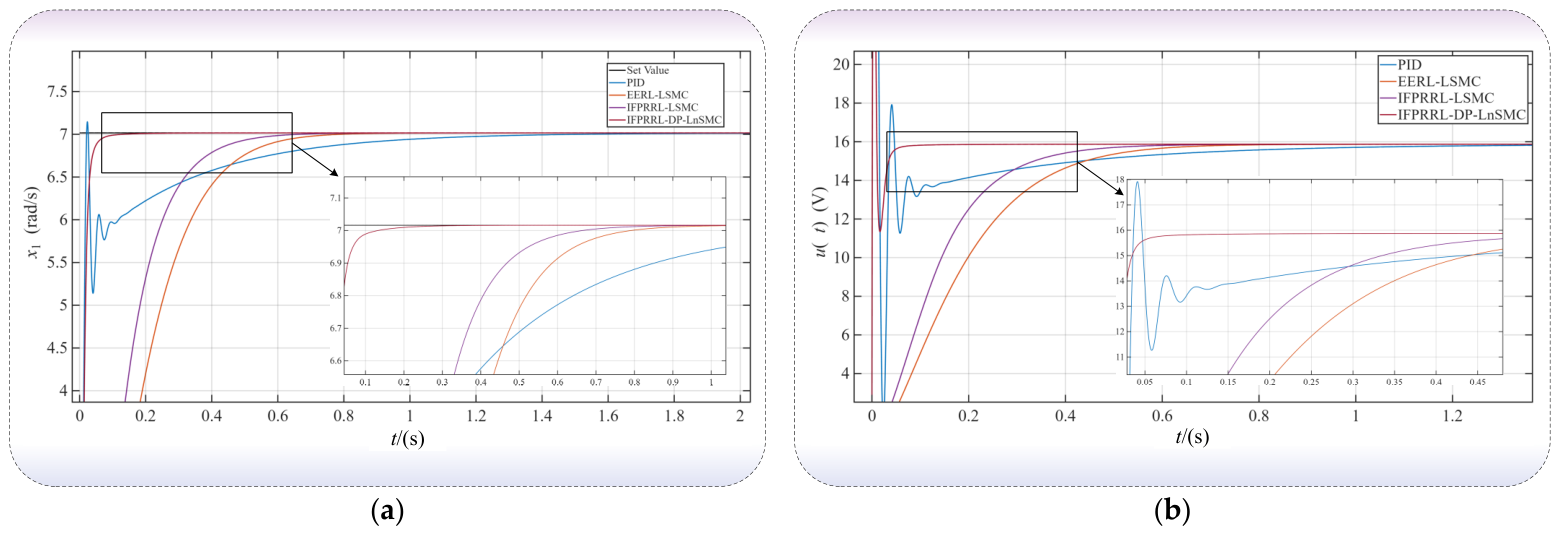
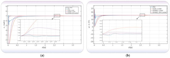
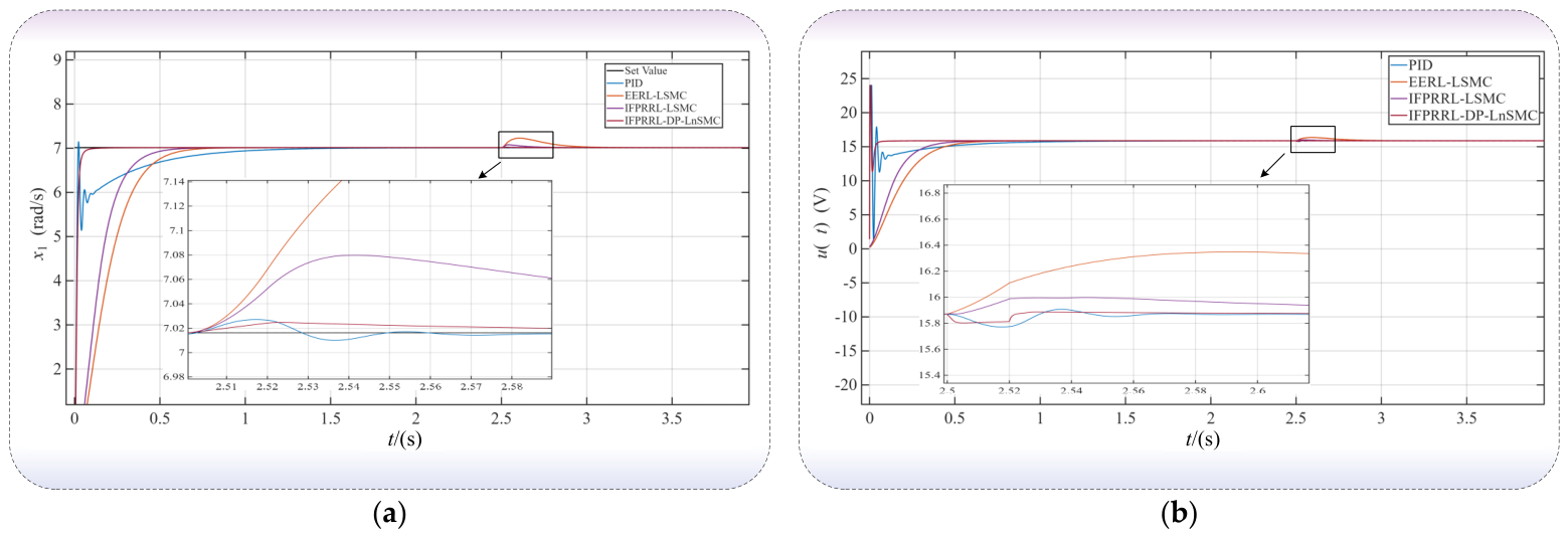
First, the DC motor model described by Equation (16) is selected as the controlled plant to evaluate the dynamic tracking performance and disturbance rejection capability of the proposed control method. The simulations are conducted in the MATLAB R2023b environment, and the motor parameters are listed in Table 2. Four control strategies, namely PID, EERL-LSMC [27], IFPRRL-LSMC [20], and the proposed IFPRRL-DP-LnSMC, are employed to regulate the motor speed for comparison. The initial angular velocity is set to 0 rads⁻¹, and the desired angular velocity is set to 7.016 rads⁻¹. The simulation results are presented in Figure 10.

Table 2. Driving Motor Parameters.

Parameter	Value	Parameter	Value
Gear reduction ratio $i_g$	47	Armature inductance $L_a$	0.01 H
Equivalent back electromotive force (EMF) constant (drive wheel side) $K_e$	2.153 Vsrad−1	Equivalent moment of inertia $J_w$	0.064 kgm2
Equivalent torque constant (drive wheel side) $K_t$	2.376 NmA−1	Viscous damping coefficient $B_w$	0.254 Nmsrad−1
Armature resistance $R_a$	1.040 Ω	Maximum input voltage $U_{\max }$	24 V

Figure 10. Angular velocity tracking performance of the driving motor under different control methods: (a) angular velocity response of the driving motor; (b) control input voltage.

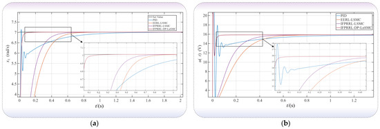
Figure 10a presents the angular velocity responses of the driving motor under different control methods. The PID controller achieves the shortest rise time of 13.6 ms; however, it exhibits an overshoot of 1.864% and requires a settling time of 787.7 ms. Both EERL-LSMC and IFPRRL-LSMC achieve overshoot-free tracking, with settling times of 565.9 ms and 449.2 ms, respectively, although their initial responses are relatively slow. In contrast, the proposed IFPRRL-DP-LnSMC achieves a rise time of 22.2 ms and a settling time of only 50 ms without noticeable overshoot. Compared with PID, EERL-LSMC, and IFPRRL-LSMC, the settling time is reduced by 93.65%, 91.16%, and 88.87%, respectively, demonstrating that the proposed dynamic power-logarithmic sliding mode surface effectively enhances the transient convergence performance of the system.

As shown in Figure 10b, both the PID controller and the proposed IFPRRL-DP-LnSMC briefly reach the maximum voltage limit of 24 V during the startup phase to achieve rapid initial acceleration. After entering the steady-state phase, the control input of the proposed method quickly converges to a stable value. The total variation of the control input after 1 s is only 1.92 × 10⁻⁷, and no significant high-frequency oscillations are observed.

To further evaluate the disturbance-rejection performance of the controller under abrupt drive-side disturbances, a rectangular pulse disturbance with an amplitude of 300 rad s⁻³ was injected into the lumped matched-disturbance channel $d_i(t)$ in Equation (13) over the interval from t = 2.500 s to t = 2.520 s. The disturbance duration was 20 ms, corresponding to a time integral of 6 rad s⁻². The same disturbance signal was applied to all comparative control methods, and the simulation results are presented in Figure 11.

Figure 11. Driving motor control performance under pulse load disturbance for different control methods: (a) angular velocity response of the driving motor; (b) control input voltage.

As shown in Figure 11a, the maximum angular velocity deviations of EERL-LSMC, IFPRRL-LSMC, PID, and IFPRRL-DP-LnSMC are 0.212, 0.064, 0.011, and 0.009 rad·s⁻¹, respectively. The proposed method exhibits the smallest peak deviation, representing reductions of 95.75%, 85.94%, and 18.18% compared with EERL-LSMC, IFPRRL-LSMC, and PID, respectively. As illustrated in Figure 11b, the peak control voltage of the proposed method is 15.886 V, which remains below the saturation limit. Moreover, the control input rapidly returns to a steady state after the disturbance is removed. These results demonstrate that the proposed IFPRRL-DP-LnSMC achieves superior overall performance in terms of response speed, tracking accuracy, control smoothness, and disturbance rejection capability.

3.2. Circular Trajectory Tracking Simulation and Analysis

After validating the inner-loop angular velocity control performance of the driving wheels, circular trajectory tracking simulations are further conducted on the double closed-loop control system of the orchard mobile robot to evaluate the effectiveness and superiority of the proposed ASTESO-DP-LnSMC control strategy for trajectory tracking.

To ensure a fair comparison, all three control schemes employ the same IFPRRL reaching law. Specifically, the compared methods include: the proposed adaptive super-twisting extended state observer-based dynamic power-logarithmic sliding mode control scheme, denoted as ASTESO-DP-LnSMC; the dynamic power-logarithmic sliding mode control scheme without ASTESO-based disturbance estimation and feedforward compensation, denoted as DP-LnSMC; and the ESO-based double closed-loop sliding mode control scheme proposed in [20], denoted as ESO-DCLSMC.

A circular reference trajectory is first selected for tracking. The center of the reference trajectory is located at (2 m, 2 m), with a radius of 7.5 m. The corresponding parametric equations are given in Equation (58). The initial pose of the orchard mobile robot in the global coordinate frame is (x₀, y₀, θ₀) = (2 m, 4 m, 0 rad), and the initial linear velocity and angular velocity are set to (v₀, w₀) = (0.60 m/s, 0.08 rad/s).

$$\left\{\begin{array}{c}{x}_d(t)=2+7.5\cos (0.08t),\hfill \\ y_d(t)=2+7.5\sin (0.08t).\hfill \end{array}\right.$$

(58)

To simulate the time-varying loads acting on the left and right wheel sets caused by variations in orchard ground adhesion, soft soil, grass-covered inter-row areas, uneven terrain, and tire slip, sustained matched load disturbances are applied to both wheel sets at t = 80 s. The simulation results of the circular trajectory tracking are presented in Figure 12.

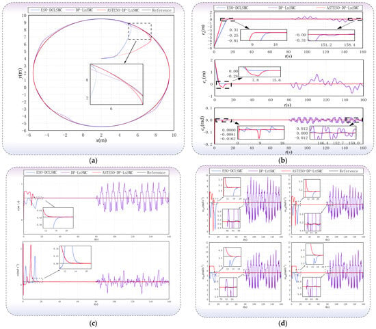
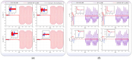
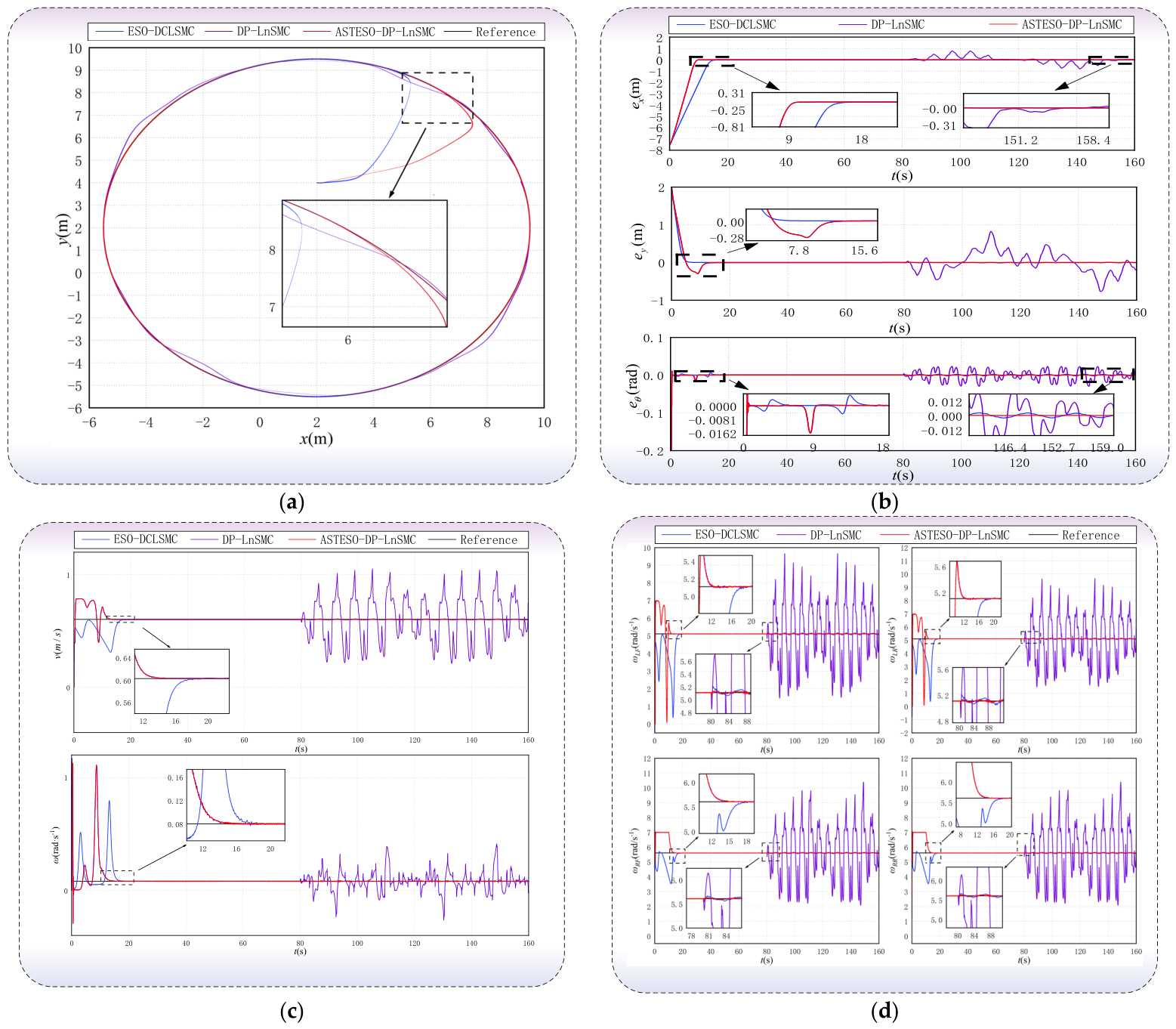
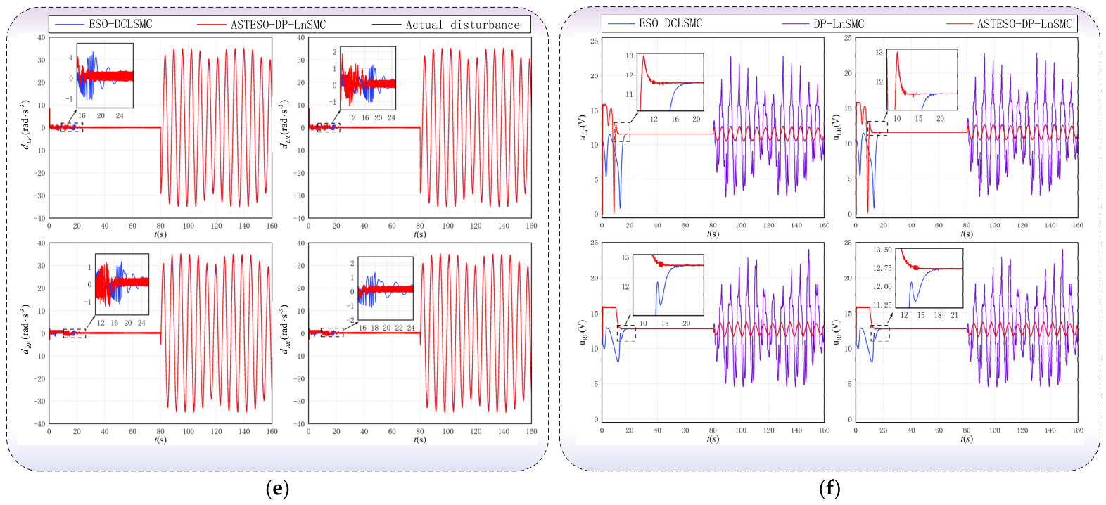
Figure 12. Comparison of circular trajectory tracking performance under different control methods: (a) circular trajectory tracking results; (b) position and heading angle tracking errors; (c) vehicle linear velocity and yaw rate responses; (d) angular velocity responses of the four driving wheels; (e) lumped disturbance estimation of the four driving wheels; (f) control input voltages of the four driving motors.

The circular trajectory tracking results are presented in Figure 12a. All three control methods are capable of driving the orchard mobile robot from its initial position toward the reference trajectory. Among them, the proposed ASTESO-DP-LnSMC achieves the fastest trajectory convergence, with a settling time of 11.560 s, representing a 24.830% reduction compared with ESO-DCLSMC. As shown in the enlarged view, before the disturbance is applied, the actual trajectory generated by the proposed method almost completely overlaps the reference trajectory. After sustained time-varying load disturbances are introduced at t = 80 s, the trajectory obtained with DP-LnSMC exhibits a noticeable deviation, whereas both ESO-DCLSMC and ASTESO-DP-LnSMC maintain stable trajectory tracking. This demonstrates that disturbance observation and feedforward compensation can effectively mitigate the influence of driving wheel load variations on the overall motion of the robot.

Figure 12b illustrates the responses of the position and heading angle tracking errors. Before the disturbance is applied, all three methods drive the tracking errors to the vicinity of zero, while ASTESO-DP-LnSMC exhibits a faster initial convergence rate and smaller transient fluctuations. After the sustained disturbance is introduced, the position and heading errors under DP-LnSMC exhibit persistent oscillations, whereas the proposed method continues to constrain both errors within a small neighborhood around zero. Table 3 summarizes the trajectory tracking error statistics for the three control methods. The position RMSE and heading angle RMSE of ASTESO-DP-LnSMC are 30.879 cm and 0.001 rad, respectively, representing reductions of 53.361% and 0.000% compared with ESO-DCLSMC, and reductions of 28.208% and 90.000% compared with DP-LnSMC. These results demonstrate that the proposed method achieves superior overall trajectory tracking accuracy.

Table 3. Statistical Results of Circular Trajectory Tracking Errors.

Algorithm	ESO-DCLSMC		DP-LnSMC		ASTESO–DP-LnSMC
	Position (cm)	Heading Angle (rad)	Position (cm)	Heading Angle (rad)	Position (cm)	Heading Angle (rad)
RMSE	66.209	0.001	43.012	0.010	30.879	0.001
Mean Error	14.014	0.001	22.131	0.007	4.644	0.000
Standard Deviation	64.710	0.001	36.882	0.008	30.528	0.001

Figure 12c,d present the responses of the vehicle body velocities and the angular velocities of the four driving wheels, respectively. Before the disturbance is applied, all control methods accurately track the desired linear velocity, yaw rate, and wheel angular velocities. After the sustained disturbance is introduced, the vehicle body velocities and driving wheel angular velocities under DP-LnSMC exhibit significant periodic oscillations, indicating that uncompensated disturbances are transmitted from the wheel-speed inner loop to the vehicle motion layer. In contrast, ASTESO-DP-LnSMC maintains stable tracking performance, with a four-wheel angular velocity RMSE of only 0.01217 rad·s⁻¹, representing reductions of 67.85% and 99.28% compared with ESO-DCLSMC and DP-LnSMC, respectively.

As shown in Figure 12e, the conventional linear ESO exhibits pronounced estimation oscillations during the initial stage, whereas the proposed ASTESO rapidly and accurately tracks the actual time-varying disturbances. Its disturbance estimation RMSE is reduced by 26.16% compared with that of the linear ESO. Figure 12f further shows that the control voltage of DP-LnSMC repeatedly reaches the 24 V saturation limit, whereas the maximum control voltage of the proposed method is only 16.1 V. Moreover, the total variation of the control input is reduced by 72.64% compared with DP-LnSMC. To quantitatively evaluate the trajectory tracking performance of the three control methods, statistical analyses of the position and heading angle errors are conducted. The proposed method achieves the smallest standard deviations for both the position and heading angle errors among the three controllers, indicating a more concentrated error distribution and superior operational consistency.

Overall, the proposed ASTESO-DP-LnSMC demonstrates superior comprehensive performance in terms of trajectory convergence speed, tracking accuracy, disturbance estimation capability, wheel-speed stability, and control input smoothness.

3.3. Real-Vehicle Experiments and Results Analysis

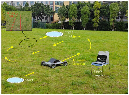
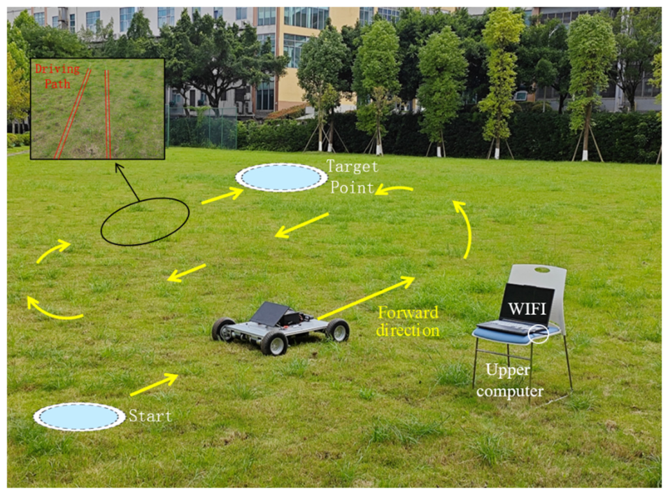
Building upon the preceding simulation studies, field experiments were further conducted to evaluate the trajectory tracking performance and practical feasibility of the proposed control method under unstructured ground conditions. The experiments were carried out in June 2025 at the outdoor test site of Chongqing University of Science and Technology, Chongqing, China. The test site is located at approximately 29°35′46″ N, 106°19′11″ E. The experimental environment and the orchard mobile robot platform are shown in Figure 13.

Figure 13. Experimental Environment.

The experiments were conducted on a natural grass field with an average vegetation height of approximately 5 cm and moderately uneven terrain. Owing to ground irregularities, vegetation coverage, and nonuniform wheel–ground contact, the orchard mobile robot is subjected to time-varying rolling resistance, variations in wheel–ground adhesion, and vehicle body attitude disturbances during motion, thereby imposing more stringent requirements on the stability and disturbance rejection capability of the trajectory tracking controller.

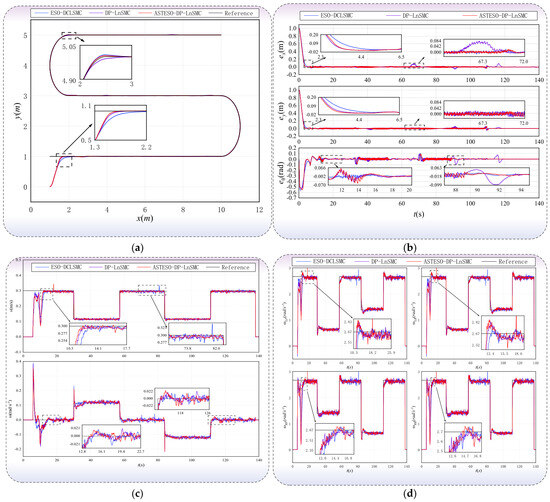
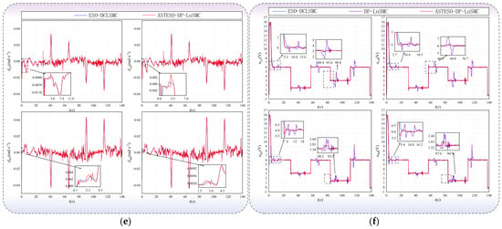
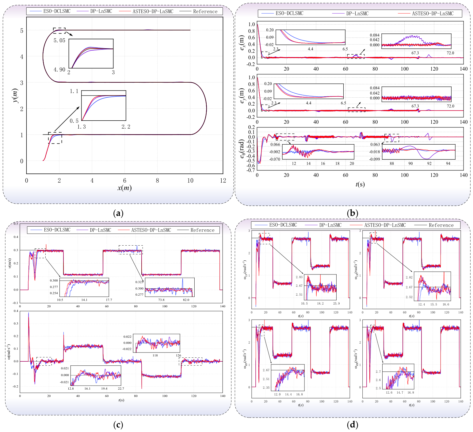
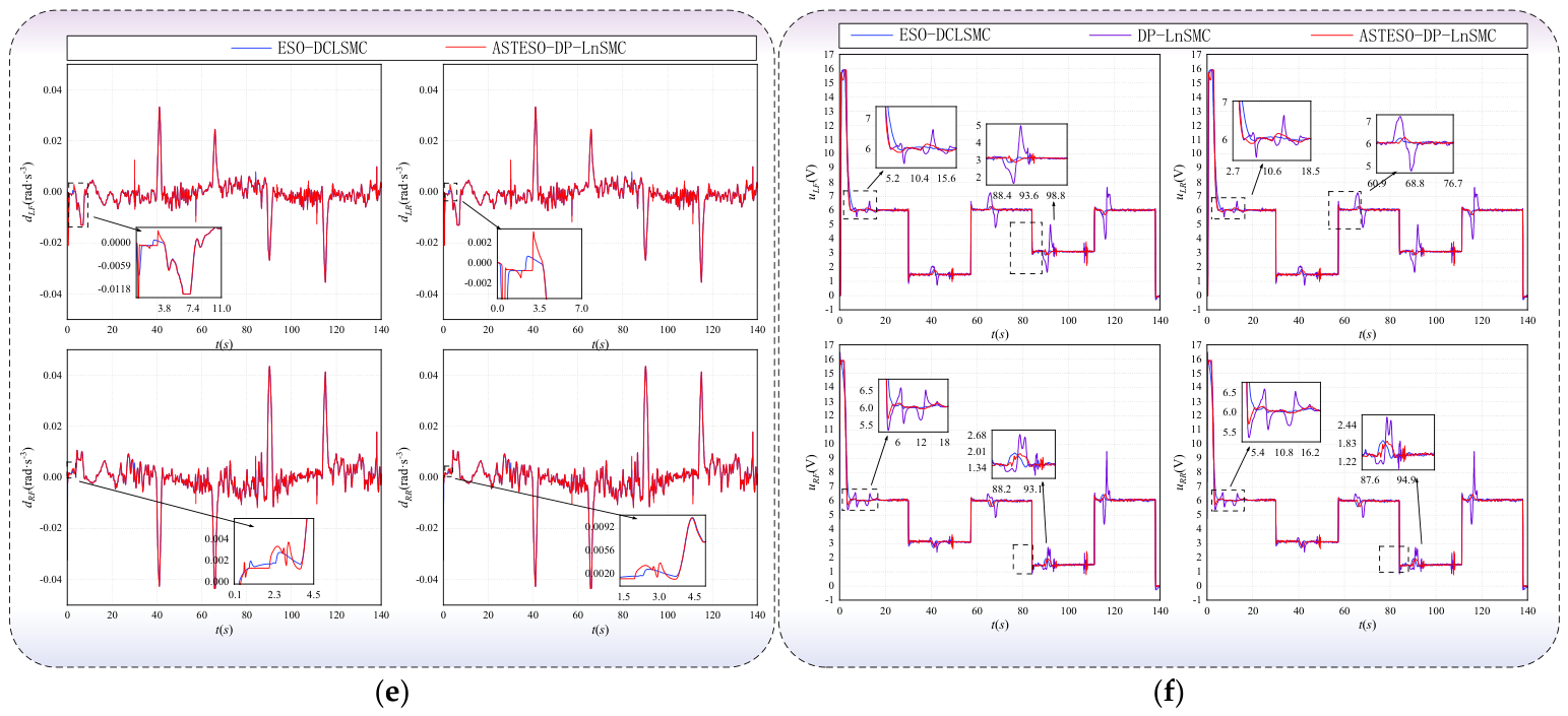
Considering that the orchard mobile robot primarily performs straight-line travel and headland turning during inter-row coverage operations, an S-shaped reference trajectory composed of multiple straight-line segments and continuous turning sections was selected for the experiments. The trajectory has a curvature of 1 m⁻¹, which simulates a typical reciprocating inter-row coverage operation in orchards. The initial pose of the orchard mobile robot was set to (0 m, 0 m, 0 rad), while the starting pose of the planned trajectory was specified as (1 m, 1 m, 0 rad). To ensure a fair comparison, ESO-DCLSMC, DP-LnSMC, and ASTESO-DP-LnSMC were all implemented on the same experimental platform using the same reference trajectory and identical initial conditions, with the control parameters individually tuned for each method. The S-shaped trajectory tracking results obtained using the three control methods are presented in Figure 14.

Figure 14. S-shaped trajectory tracking experimental results on a grass field under different control methods: (a) trajectory tracking results; (b) position and heading angle tracking errors; (c) vehicle linear velocity and angular velocity responses; (d) angular velocity responses of the four driving wheels; (e) lumped disturbance estimation of the four driving wheels; (f) control input voltages of the four driving motors.

Figure 14a presents the S-shaped trajectory tracking results obtained using the three control methods. All methods successfully drive the robot from its initial position toward the reference trajectory and accomplish both straight-line motion and continuous headland turning. As shown in the enlarged view, ASTESO-DP-LnSMC exhibits the fastest convergence during the initial trajectory acquisition stage and maintains a high degree of overlap with the reference trajectory throughout the subsequent straight-line and turning segments. In contrast, ESO-DCLSMC and DP-LnSMC exhibit more pronounced transient deviations during the initial trajectory acquisition phase and in regions where the path curvature changes.

Figure 14b illustrates the longitudinal position error, lateral position error, and heading angle error responses. Owing to the initial pose mismatch, all tracking errors exhibit relatively large transient variations during the startup phase before rapidly converging to the vicinity of zero. During the turning and velocity switching intervals, approximately 67–72 s and 88–95 s, the error responses undergo short-duration fluctuations but quickly return to a small range. ASTESO-DP-LnSMC consistently exhibits smaller error magnitudes during both the initial convergence and turning phases, indicating that the adaptive disturbance estimation and feedforward compensation effectively suppress error accumulation caused by variations in ground adhesion, rolling resistance, and unmodeled dynamics.

Figure 14c,d show the responses of the vehicle linear velocity, angular velocity, and the angular velocities of the four driving wheels, respectively. The actual vehicle velocities accurately track the piecewise-varying reference commands, with only brief fluctuations occurring during startup, acceleration/deceleration, and steering transitions. All four driving wheels rapidly track their corresponding desired angular velocities, while the left and right wheel sets automatically generate the differential wheel speed required for differential steering during turning, demonstrating that the inner-loop controller accurately executes the vehicle velocity commands generated by the outer-loop controller.

As shown in Figure 14e, the estimated lumped disturbances of the four drive wheels obtained by ESO-DCLSMC and ASTESO-DP-LnSMC exhibit pronounced dynamic variations during vehicle acceleration, deceleration, steering, and changes in wheel–ground contact conditions. The timing of these variations is generally consistent with the transient fluctuations observed in the vehicle linear and angular velocities and in the angular velocities of the four drive wheels, indicating that the observers can respond dynamically to equivalent disturbances associated with changes in the operating state of the drive system and wheel–ground interaction. It should be emphasized that, under the current real-vehicle experimental configuration, no independent force- or torque-based sensing system is available to directly obtain the true lumped disturbances $d_i(t)$. Therefore, all curves shown in Figure 14e represent observer-based lumped-disturbance estimates rather than independently measured disturbance ground truth. Accordingly, Figure 14e is used primarily for a qualitative comparison of the dynamic response characteristics of the observers during real-vehicle operation, rather than for a quantitative assessment of disturbance-estimation error or estimation accuracy relative to the unknown true disturbances.

Table 4 summarizes the quantitative performance evaluation results for the three control methods. The proposed ASTESO-DP-LnSMC achieves a position RMSE of 10.512 cm, representing reductions of 29.775% and 36.880% compared with ESO-DCLSMC and DP-LnSMC, respectively. Its mean position error is 2.172 cm, corresponding to reductions of 21.018% and 53.089%, respectively. The heading angle RMSE is 0.050 rad, which is reduced by 24.698% and 42.171% compared with the two reference methods, while the mean heading angle error is 0.016 rad, corresponding to reductions of 53.527% and 58.786%, respectively. Furthermore, the proposed method achieves the smallest standard deviations for both the position and heading angle errors among the three control methods, indicating a more concentrated error distribution and better operational consistency.

Table 4. Statistical Results of Trajectory Tracking Errors.

Algorithm	ESO-DCLSMC		DP-LnSMC		ASTESO–DP-LnSMC
	Position (cm)	Heading Angle (rad)	Position (cm)	Heading Angle (rad)	Position (cm)	Heading Angle (rad)
RMSE	14.969	0.066	16.654	0.086	10.512	0.050
Mean Error	2.750	0.034	4.630	0.038	2.172	0.016
Standard Deviation	14.747	0.064	16.378	0.083	10.322	0.048

Overall, ASTESO-DP-LnSMC maintains high trajectory tracking accuracy and stable driving wheel speed responses under natural grass terrain, uneven ground surfaces, and uncertain wheel–ground contact conditions, thereby validating the disturbance rejection capability and practical engineering feasibility of the proposed control method.

4. Conclusions

This study addresses the degradation of wheel-speed tracking performance and vehicle trajectory deviations of orchard mobile robots operating on unstructured terrain due to variations in wheel–ground contact, drive-load disturbances, and model uncertainties. A composite control method based on an adaptive super-twisting extended state observer and dynamic power–logarithmic sliding-mode control (ASTESO–DP-LnSMC) is proposed. By establishing a kinematic model of the mobile robot and a dynamic model of the drive-wheel motors incorporating lumped disturbances, a cascaded control system consisting of an outer-loop vehicle kinematic controller and an inner-loop drive-wheel speed controller is constructed. The ASTESO is employed to estimate the angular acceleration of the drive wheels and the lumped disturbances arising from load variations, parameter perturbations, and unmodeled dynamics in real time, and the resulting estimates are further used for feedforward compensation in wheel-speed control. Dynamic power–logarithmic sliding-mode control is employed to improve the transient response, steady-state tracking accuracy, and smoothness of the control input for the drive wheels. Theoretical analysis demonstrates that, under the assumptions specified in this study, the observation errors converge in finite time; in the presence of bounded disturbance-estimation residuals, the drive-wheel speed tracking errors remain uniformly ultimately bounded.

Drive-system simulation results show that the settling time of the drive-wheel angular velocity under the proposed method is 50 ms, and the maximum angular-velocity deviation under the prescribed pulse load disturbance is 0.009 rad s⁻¹, indicating that the proposed method can effectively suppress the influence of drive-side load disturbances on wheel-speed tracking. Based on the full-vehicle simulations, field experiments involving an S-shaped trajectory were further conducted on a natural grass-covered site with moderate surface undulations to emulate reciprocating inter-row coverage operations. In the field experiments, the position and heading-angle RMSEs of ASTESO–DP-LnSMC were 10.512 cm and 0.050 rad, respectively; compared with ESO–DCLSMC, they were reduced by 29.78% and 24.70%, respectively, and compared with DP–LnSMC, they were reduced by 36.88% and 42.17%, respectively. These results demonstrate that, under the outdoor unstructured conditions evaluated in this study, including natural grass-covered terrain, surface undulations, and variations in wheel–ground contact, the proposed method maintains favorable trajectory-tracking accuracy and drive-wheel speed stability.

It should be noted that the current field experiments were conducted on natural grass-covered terrain using trajectories designed to emulate orchard inter-row operations and did not cover operating conditions encountered in real orchards, such as different soil types, slopes, pronounced longitudinal and lateral slip, and long-term continuous operation. Therefore, the conclusions of this study are primarily applicable to the experimentally validated conditions described above and are not extrapolated to complex orchard operating conditions that have not yet been tested. Future work will further account for longitudinal and lateral slip as well as tire–soil coupling characteristics, investigate online adaptive tuning of observer and controller parameters, and conduct long-term experiments in real orchards under different terrain, speed, and load conditions to further evaluate the adaptability of the proposed method to varying operating conditions and its engineering applicability.

References

- Vougioukas, S.G. Agricultural Robotics. Annu. Rev. Control Robot. Auton. Syst. 2019, 2, 365–392. [Google Scholar] [CrossRef] [Scilit]
- Opiyo, S.; Okinda, C.; Zhou, J.; Mwangi, E.; Makange, N. Medial axis-based machine-vision system for orchard robot navigation. Comput. Electron. Agric. 2021, 185, 106153. [Google Scholar] [CrossRef] [Scilit]
- Ye, L.; Wu, F.; Zou, X.; Li, J. Path planning for mobile robots in unstructured orchard environments: An improved kinematically constrained bi-directional RRT approach. Comput. Electron. Agric. 2023, 215, 108453. [Google Scholar] [CrossRef] [Scilit]
- Moriones Polanía, E.C.; Fernandes, H.R.; Albiero, D.; Garcia, A.P. Control System for the Navigation of the Agricultural Robots: A Review. J. Field Robot. 2026, 43, 3474–3505. [Google Scholar] [CrossRef] [Scilit]
- Yang, Y.; Li, Y.; Wen, X.; Zhang, G.; Ma, Q.; Cheng, S.; Qi, J.; Xu, L.; Chen, L. An optimal goal point determination algorithm for automatic navigation of agricultural machinery: Improving the tracking accuracy of the Pure Pursuit algorithm. Comput. Electron. Agric. 2022, 194, 106760. [Google Scholar] [CrossRef] [Scilit]
- Zhang, S.; Wei, X.; Liu, C.; Ge, J.; Cui, X.; Wang, F.; Wang, A.; Chen, W. Adaptive path tracking and control system for unmanned crawler harvesters in paddy fields. Comput. Electron. Agric. 2025, 230, 109878. [Google Scholar] [CrossRef] [Scilit]
- Hu, Q.; Fan, Z.; Zhang, X.; Sun, N.; Li, X.; Qiu, Q. Robust localization and tracking control of high-clearance robot system servicing high-throughput wheat phenotyping. Comput. Electron. Agric. 2025, 229, 109793. [Google Scholar] [CrossRef] [Scilit]
- Graf Plessen, M.M.; Bemporad, A. Reference trajectory planning under constraints and path tracking using linear time-varying model predictive control for agricultural machines. Biosyst. Eng. 2017, 153, 28–41. [Google Scholar] [CrossRef] [Scilit]
- Zhang, T.; Jiao, X.; Lin, Z. Finite time trajectory tracking control of autonomous agricultural tractor integrated nonsingular fast terminal sliding mode and disturbance observer. Biosyst. Eng. 2022, 219, 153–164. [Google Scholar] [CrossRef] [Scilit]
- Ding, C.; Ding, S.; Wei, X.; Mei, K. Output feedback sliding mode control for path-tracking of autonomous agricultural vehicles. Nonlinear Dyn. 2022, 110, 2429–2445. [Google Scholar] [CrossRef] [Scilit]
- Li, J.; Shang, Z.; Li, R.; Cui, B. Adaptive Sliding Mode Path Tracking Control of Unmanned Rice Transplanter. Agriculture 2022, 12, 1225. [Google Scholar] [CrossRef] [Scilit]
- Luo, Y.; Pu, D.; He, X.; Song, L.; Yang, S.X.; Ma, W.; Shi, H. Trajectory Tracking Control of an Orchard Robot Based on Improved Integral Sliding Mode Algorithm. Agriculture 2025, 15, 1881. [Google Scholar] [CrossRef] [Scilit]
- Lee, H.; Utkin, V.I. Chattering suppression methods in sliding mode control systems. Annu. Rev. Control 2007, 31, 179–188. [Google Scholar] [CrossRef] [Scilit]
- Zhao, L.; Li, J.; Li, H.; Liu, B. Double-loop tracking control for a wheeled mobile robot with unmodeled dynamics along right angle roads. ISA Trans. 2023, 136, 525–534. [Google Scholar] [CrossRef] [Scilit] [PubMed]
- Lu, E.; Xue, J.; Chen, T.; Jiang, S. Robust Trajectory Tracking Control of an Autonomous Tractor-Trailer Considering Model Parameter Uncertainties and Disturbances. Agriculture 2023, 13, 869. [Google Scholar] [CrossRef] [Scilit]
- Chen, W.H.; Yang, J.; Guo, L.; Li, S. Disturbance-Observer-Based Control and Related Methods—An Overview. IEEE Trans. Ind. Electron. 2016, 63, 1083–1095. [Google Scholar] [CrossRef] [Scilit]
- Sun, J.; Wang, Z.; Ding, S.; Xia, J.; Xing, G. Adaptive disturbance observer-based fixed time nonsingular terminal sliding mode control for path-tracking of unmanned agricultural tractors. Biosyst. Eng. 2024, 246, 96–109. [Google Scholar] [CrossRef] [Scilit]
- Zhang, Y.; Shen, Y.; Liu, H.; He, S.; Khan, Z. A composite sliding mode controller with extended disturbance observer for 4WSS agricultural robots in unstructured farmlands. Comput. Electron. Agric. 2025, 232, 110069. [Google Scholar] [CrossRef] [Scilit]
- Shtessel, Y.; Taleb, M.; Plestan, F. A novel adaptive-gain supertwisting sliding mode controller: Methodology and application. Automatica 2012, 48, 759–769. [Google Scholar] [CrossRef] [Scilit]
- Song, L.; Huang, J.; Liang, Q.; Nie, L.; Liang, X.; Zhu, J. Trajectory Tracking Strategy for Sliding Mode Control With Double Closed-Loop for Lawn Mowing Robot Based on ESO. IEEE Access 2023, 11, 1867–1882. [Google Scholar] [CrossRef] [Scilit]
- Yamasaki, Y.; Ishii, K.; Noguchi, N. Speed control of an autonomous electric vehicle for orchard spraying. Comput. Electron. Agric. 2025, 236, 110419. [Google Scholar] [CrossRef] [Scilit]
- Liao, J.; Chen, Z.; Yao, B. Model-Based Coordinated Control of Four-Wheel Independently Driven Skid Steer Mobile Robot with Wheel–Ground Interaction and Wheel Dynamics. IEEE Trans. Ind. Inform. 2019, 15, 1742–1752. [Google Scholar] [CrossRef] [Scilit]
- Hou, Q.; Ding, S. Finite-Time Extended State Observer-Based Super-Twisting Sliding Mode Controller for PMSM Drives With Inertia Identification. IEEE Trans. Transp. Electrif. 2022, 8, 1918–1929. [Google Scholar] [CrossRef] [Scilit]
- Cui, L.; Zhang, R.; Yang, H.; Zuo, Z. Adaptive super-twisting trajectory tracking control for an unmanned aerial vehicle under gust winds. Aerosp. Sci. Technol. 2021, 115, 106833. [Google Scholar] [CrossRef] [Scilit]
- Xin, J.; Xinhua, W.; Anzhe, W.; Bingbo, C.; Qi, S. A novel composite adaptive terminal sliding mode controller for farm vehicles lateral path tracking control. Nonlinear Dyn. 2022, 110, 2415–2428. [Google Scholar] [CrossRef] [Scilit]
- Wu, Y.; Wang, L.; Zhang, J.; Li, F. Path Following Control of Autonomous Ground Vehicle Based on Nonsingular Terminal Sliding Mode and Active Disturbance Rejection Control. IEEE Trans. Veh. Technol. 2019, 68, 6379–6390. [Google Scholar] [CrossRef] [Scilit]
- Mozayan, S.M.; Saad, M.; Vahedi, H.; Fortin-Blanchette, H.; Soltani, M. Sliding Mode Control of PMSG Wind Turbine Based on Enhanced Exponential Reaching Law. IEEE Trans. Ind. Electron. 2016, 63, 6148–6159. [Google Scholar] [CrossRef] [Scilit]
Disclaimer/Publisher’s Note: The statements, opinions and data contained in all publications are solely those of the individual author(s) and contributor(s) and not of MDPI and/or the editor(s). MDPI and/or the editor(s) disclaim responsibility for any injury to people or property resulting from any ideas, methods, instructions or products referred to in the content. |
© 2026 by the authors. Licensee MDPI, Basel, Switzerland. This article is an open access article distributed under the terms and conditions of the Creative Commons Attribution (CC BY) license.