


Abstract
Autonomous headland operations require reliable boundary perception and timely behavioral decisions in unstructured field environments. This study proposes a perception-and-decision framework for autonomous agricultural machinery. A CA-SP-DeepLabV3+ semantic segmentation model is developed by integrating Coordinate Attention, Strip Pooling, and a combined Boundary–Dice loss to enhance the continuity and localization of weak and elongated headland boundaries. To facilitate deployment on resource-constrained computing platforms, structured pruning and knowledge distillation are further applied to compress the segmentation network. A stereo-vision-based three-dimensional boundary reconstruction method is then used to estimate the vehicle-relative distance to the headland boundary. Based on the estimated distance, tractor–implement parameters, operating speed, and selected turn type, the decision module calculates the required headland width and distance thresholds for deceleration and turn preparation. Experimental results show that the compressed segmentation model achieved IoU values of 92.55% and 96.53% for the headland and field classes, respectively, while reducing the number of parameters and FLOPs by 28.48% and 48.43% compared with the uncompressed model. Across four representative headland environments and reference distances ranging from 10 to 30 m, the relative ranging errors ranged from 1.30% to 7.03%, and the total processing latency remained below 45.5 ms under the evaluated conditions. The decision experiments further showed that the proposed method generated headland-width plans and deceleration thresholds consistent with the geometric and kinematic constraints of different tractor–implement combinations and operating conditions. These results support the feasibility of the proposed framework for boundary perception, distance estimation, and behavioral decision support under the evaluated conditions.
1. Introduction
Agricultural machinery is indispensable for modern agricultural production. Driven by continuous technological innovation, automatic navigation systems have been widely commercialized, successfully enabling the semi-automation of field operations. Nevertheless, when approaching field headlands, human intervention remains necessary for turning maneuvers and the lifting or lowering of implements. Consequently, there is a growing consensus on the need to further enhance the intelligence of agricultural machinery and develop fully autonomous driving technologies [1,2,3]. Within this context, headland environment recognition and behavioral decision-making represent critical underlying technologies [4,5,6].
In the field of headland image recognition, earlier studies predominantly employed traditional manual feature extraction methods. Li et al. [7] distinguished crops from headland boundaries based on farmland color and texture. Wang et al. [8] identified headlands by detecting pixel intensity transitions between the field and its surroundings, accurately locating boundary lines through sub-regional greyscale distribution analysis. Qiao et al. [9] proposed a detection method specifically for grayscale mutation headland images by partitioning the image into eight horizontal regions, identifying feature points within each, and extracting boundaries via robust regression. However, in complex real-world farmland scenarios, traditional machine vision algorithms struggle with illumination fluctuations, shadows, and blurred boundaries, leading to limited generalization and robustness.
Deep learning-based vision technologies are capable of learning hierarchical and complex features from large-scale headland image training data and have thus become the primary method for headland detection research. Qiao et al. [10] employed a compact MobileNetV2 architecture to achieve automatic recognition of six types of farmland headland images. Liu et al. [11] developed a headland boundary recognition and ranging system based on deep learning and binocular vision, enabling real-time detection and distance measurement. He et al. [12] utilized MobileV2-UNet to achieve pixel-level semantic segmentation of rice field boundary areas and introduced the random sample consensus (RANSAC) algorithm for linear fitting of boundary pixels. Ji et al. [13] acquired two-dimensional texture and three-dimensional depth information of farmland scenes via RGB-D images, employing an improved YOLOv5-seg model to extract headland contours and determining boundary distances by integrating depth information. Li et al. [14] fused multi-modal and temporal features from continuous RGB-D images to implement headland boundary detection based on a hybrid deep neural network.
After the task of headland recognition, the existing literature has largely focused on steering path planning and decision-making. Unlike global coverage path planning [15,16], this constitutes a local path planning task. He et al. [17] proposed a dynamic turning path planning method for a four-wheeled vehicle platform using an asymmetric turn-back steering strategy, effectively shortening the path length and improving operational efficiency. Furthermore, Wu et al. [18] fused multi-modal features from RGB-D images to achieve headland boundary detection using an improved DeepLabv3+. They then generated autonomous steering paths for agricultural robots by combining multi-order Bézier curves with the boundary’s curvature change points. Liu et al. [19] combined BiSeNet-based segmentation with GNSS positioning for rice transplanter navigation. Their system used the distance to headland ridges in world coordinates to support autonomous row-switching and path tracking.
Backman et al. [20] generated headland turning paths with continuous curvature and speed while accounting for steering-rate and acceleration constraints. Chen et al. [21] evaluated turning types in terms of path length, turning time, and required headland width while considering harvester geometry. Building on these studies, this work develops and evaluates a vision-based framework focused on distance-triggered pre-turn decisions. The methodological contribution is to link visual headland perception and stereo distance estimation directly to behavioral decision thresholds. These thresholds account for tractor–implement geometry and deceleration requirements to determine when to slow down and prepare for turning.
The main contributions are as follows: (1) A trigger-based perception framework uses MobileNetV4-Small to classify scenes and activate semantic segmentation and stereo ranging when a headland is detected. This conditional processing strategy is designed to reduce onboard computational demands. (2) A boundary-oriented CA-SP-DeepLabV3+ model integrates Coordinate Attention, Strip Pooling, and a combined Boundary and Dice loss to segment weak and elongated headland boundaries. Structured pruning and knowledge distillation are applied to balance segmentation accuracy and computational cost. (3) A distance-threshold-based decision method combines stereo-derived boundary distance with tractor–implement geometry, operating speed, deceleration requirements, and the selected turning pattern. It calculates the required headland width and thresholds for continued operation, deceleration, and turn preparation, providing decision-level inputs for subsequent implement and steering control.
2. Materials and Methods
2.1. System Overview
2.1.1. Hardware Configuration
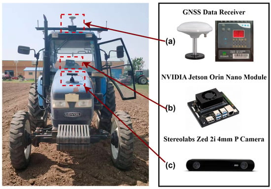
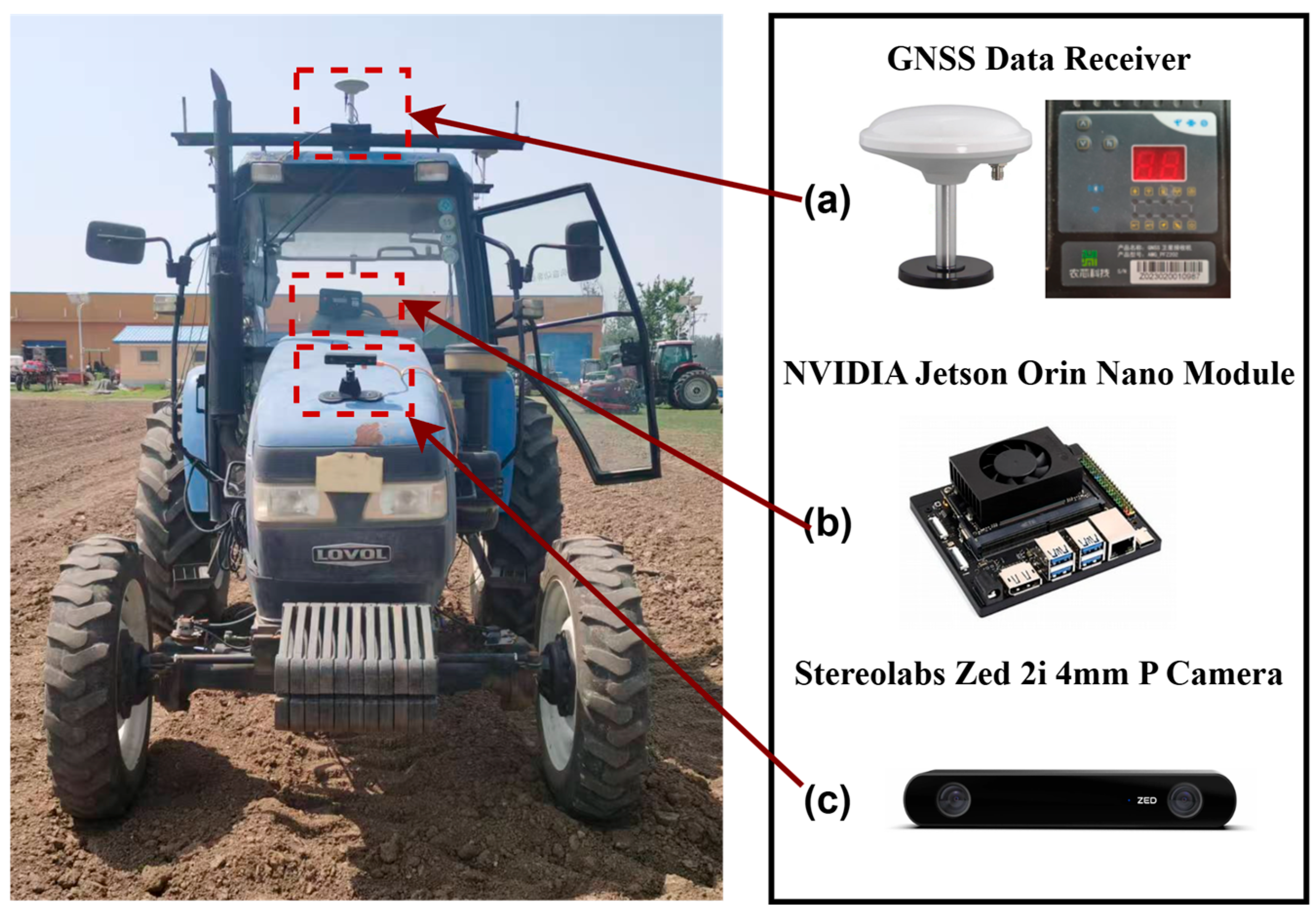
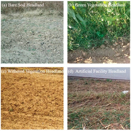
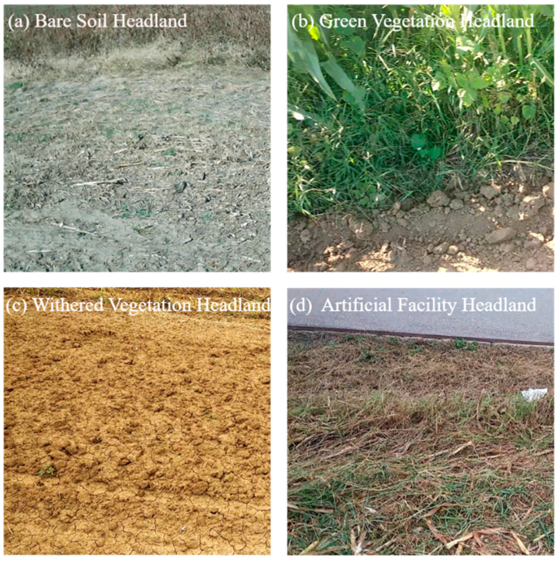
A tractor-mounted sensing and computing system was developed for data collection and field experiments conducted in 2025 at the Xiaotangshan National Precision Agriculture Demonstration Base in Beijing, China. Figure 1 shows the composition and installation layout of the system. A ZED 2i stereo depth camera (Stereolabs Inc., San Francisco, CA, USA) with a 4 mm lens and polarizing filter was mounted at the tractor front. The camera was positioned approximately 1.3 m above the ground at a 30° pitch angle and had a maximum detection range of approximately 40 m. A Jetson Orin Nano installed in the cab acquired and processed camera and GNSS receiver data in real time. Field experiments covered four representative headland environments: bare soil, green vegetation, withered vegetation, and artificial facilities, as shown in Figure 2.
Figure 1.
Experimental setup for device installation and data acquisition.
Figure 2.
Image of a typical headland environment.
2.1.2. System Workflow
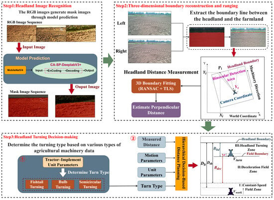
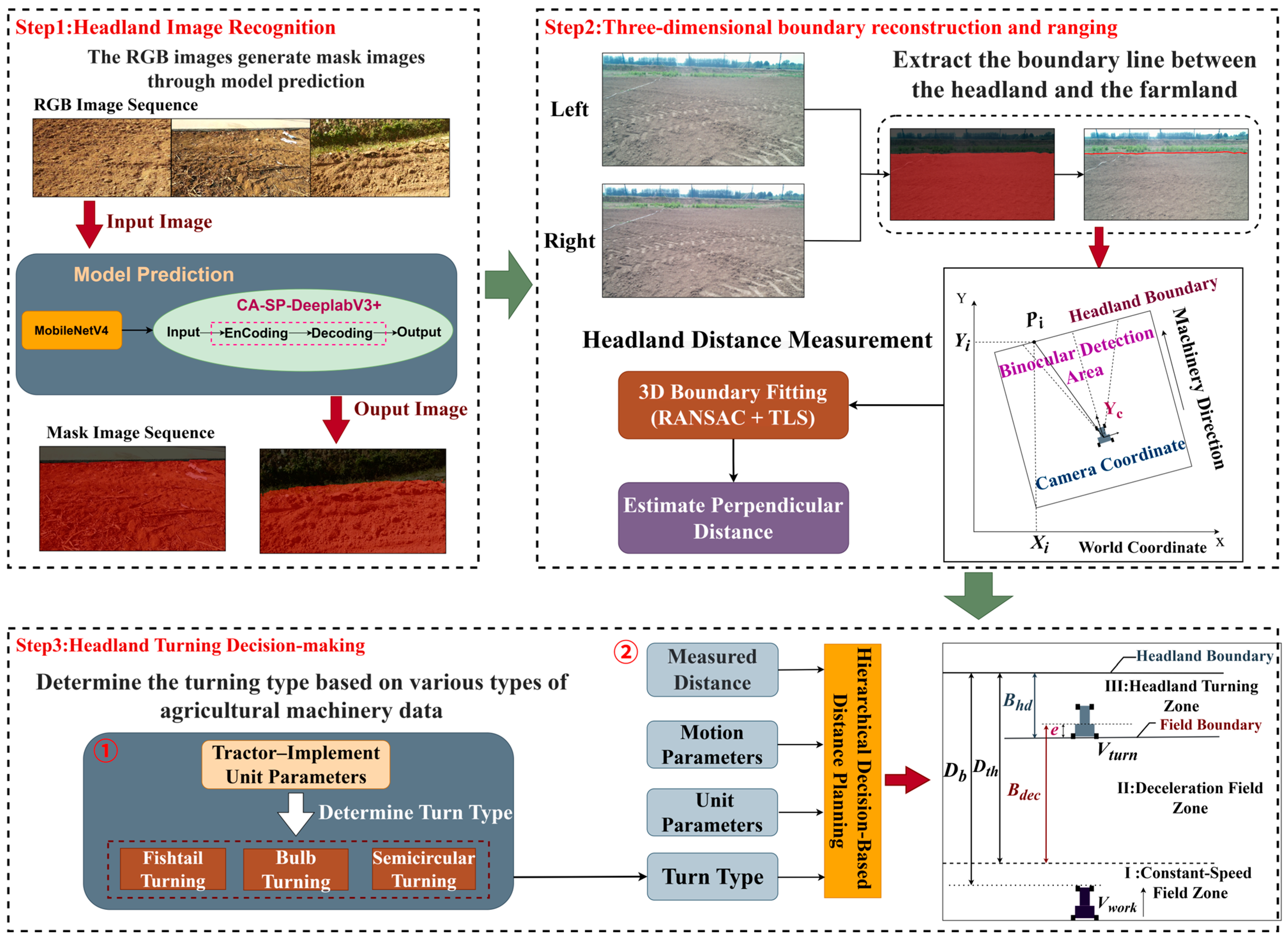
The proposed method comprises three stages: headland recognition, boundary extraction and ranging, and headland turning decision-making, as shown in Figure 3.
Figure 3.
Overall workflow of this study.
Step 1: Headland Image Recognition
MobileNetV4-Small classifies each image as headland or land. When a headland is detected, CA-SP-DeepLabV3+ segments the image into working farmland and headland regions.
Step 2: Three-dimensional boundary reconstruction and ranging
Stereo depth is associated with the segmented boundary pixels to reconstruct three-dimensional boundary points. Invalid observations and geometric outliers are removed using validity filtering and RANSAC. The retained points are refitted by total least squares, and the vehicle-relative headland distance is calculated as the perpendicular distance from the camera center to the fitted local boundary.
Step 3: Headland Behavioral Decision-making
The decision module selects a turning mode according to the machine and implement parameters and calculates the required headland width. It then combines the measured headland distance with the machine motion parameters to determine the deceleration and turning thresholds. These thresholds govern the transitions between approach, deceleration, and turning behaviors.
2.2. Headland Image Recognition
2.2.1. Dataset Construction
Images were obtained from agricultural sites across China, covering four headland environments: bare soil, green vegetation, withered vegetation, and artificial facilities. Manual screening removed blurred, severely overexposed or underexposed, corrupted, and visually highly similar images to improve image quality, reduce redundancy, and mitigate the risk of data leakage arising from similar images of the same field appearing in different subsets. The classification dataset comprised 7500 images, including 5000 headland and 2500 non-headland images. A subset of 1300 headland images was used for semantic segmentation, with pixel-level annotations for headland and working farmland. The 1300 annotated images were divided into training, validation, and test subsets containing 910, 260, and 130 images, respectively, at a ratio of 7:2:1.
Weather-related changes in illumination and visibility may affect both boundary segmentation and stereo ranging. Strong shadows, fog, and rain may obscure boundary features, while reflections from wet surfaces may impair stereo matching. Invalid depth filtering and RANSAC reduce unreliable observations.
2.2.2. Two-Stage Headland Recognition Method
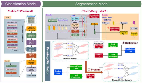
To address the limited computational power and real-time requirements of agricultural machinery on-board terminals, a two-stage detect-then-segment headland recognition framework was designed, as shown in Figure 4. In the first stage, MobileNetV4-Small was used as a lightweight trigger model to rapidly classify each forward-looking image as either “headland” or “land” [22]. Only the frames identified as headland scenes were passed to the second-stage segmentation network, thereby avoiding continuous execution of the high-complexity segmentation model on irrelevant field images.
Figure 4.
The proposed two-stage framework for headland recognition.
For pixel-level boundary perception, a boundary-oriented CA-SP-DeepLabV3+ model was constructed [23]. The Coordinate Attention mechanism was used to enhance position-sensitive feature representation, while Strip Pooling was integrated into the ASPP module to capture long-range contextual information along slender headland boundaries. In addition, a combined Boundary and Dice loss was adopted to improve both regional overlap and boundary alignment. These modifications were introduced to adapt the segmentation model to the weak-texture, elongated, and irregular characteristics of headland boundaries.
After training, structured pruning and knowledge distillation were applied to compress the segmentation network [24]. The compressed student model was optimized to reduce parameters, FLOPs, and inference latency while preserving boundary localization accuracy. Therefore, the proposed recognition framework was evaluated not only by segmentation accuracy, but also by trigger reliability, computational efficiency, and boundary-preserving performance.
2.2.3. Boundary-Aware Enhancement Modules for Headland Segmentation
After the headland scene is detected by the first-stage classifier, a boundary-oriented CA-SP-DeepLabV3+ model is activated for pixel-level semantic segmentation. This stage aims to distinguish the working farmland region from the headland region and provide semantic masks for subsequent boundary extraction, three-dimensional reconstruction, and distance estimation.
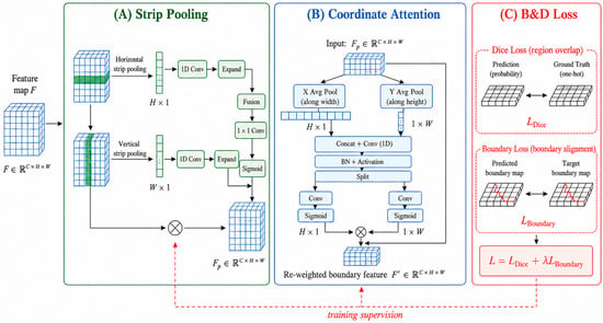
As shown in Figure 5, three task-specific enhancement modules are introduced to improve boundary perception [25]. Headland boundary segmentation differs from general semantic segmentation because the boundary is usually slender, elongated, weakly textured, and easily affected by uneven illumination, crop residues, and vegetation. As shown in Figure 4, Strip Pooling is added as a sixth parallel ASPP branch, retaining the original five branches. Input channels are reduced to one quarter before adaptive average pooling generates 1 × W and H × 1 feature maps, followed by 1 × 3 and 3 × 1 convolutions, respectively. The outputs are bilinearly resized, summed, and refined by a 3 × 3 convolutional block. A 1 × 1 convolution restores the channel dimension before residual addition and ReLU. The resulting features are projected to 256 channels, concatenated with the other five branch outputs, and fused into 256 channels using a 1 × 1 convolutional block. Seven CA modules are placed after batch normalization and ReLU in the four ASPP convolutional branches, the ASPP fusion block, the low-level feature projection, and the second decoder convolutional block [26]. Their channel reduction ratios are 8 for the five ASPP modules, 4 for the low-level projection, and 16 for the decoder module. Directional average pooling and a shared 1 × 1 convolutional block encode positional information, followed by separate projections and sigmoid activations that generate two attention maps to reweight the input features. In addition, a combined Boundary–Dice loss is adopted to jointly optimize regional overlap and boundary alignment, as defined in Equation (1) [27,28]:
where measures mask overlap and constrains boundary alignment. The weighting parameter was fixed at 0.5 throughout the original model training.
Figure 5.
Boundary-aware enhancement modules in DeepLabV3+ for headland segmentation.
2.2.4. Lightweight Training and Model Compression
To ensure the fairness and reproducibility of model training and comparison, all segmentation models were implemented using the PyTorch 2.1.2 framework and trained on a workstation equipped with an Intel Core i9-12900HX CPU (Intel Corporation, Santa Clara, CA, USA) and an NVIDIA GeForce RTX 4090 GPU (NVIDIA Corporation, Santa Clara, CA, USA). The segmentation dataset was divided into training, validation, and test sets at a ratio of 7:2:1, and all input images were resized to 512 × 512 pixels. The proposed model and all comparison models were trained for 200 epochs using the SGD optimizer with a batch size of 16. The initial learning rate was set to 0.007 and adjusted using a cosine annealing strategy. The same dataset partition, input resolution, and training protocol were used for all models to ensure a consistent experimental comparison. Each segmentation configuration was trained independently 10 times using different random seeds, while keeping the training, validation, and test split unchanged. Each trained model was evaluated on the same test set of 130 images.
After training, first-order Taylor-based structured channel pruning was applied primarily to the MobileNetV2 backbone and the shortcut conv and cat conv modules in the decoder. Pruning was performed progressively over three stages, with a target channel-pruning ratio of 30%. After each stage, the pruned model was fine-tuned for five epochs using cross-entropy loss and the Adam optimizer, with an initial learning rate of 1 × 10⁻⁴ and a batch size of 4.
The uncompressed model served as the teacher and the pruned model as the student for hybrid knowledge distillation combining soft-label and relational supervision. The teacher remained in evaluation mode with its parameters frozen. The student learned from the teacher’s segmentation outputs and the distance and angle relationships among output representations, with a soft-label distillation temperature of 2. The training objective combined Boundary loss, Dice loss, relational distillation loss, and soft-label KL-divergence loss, weighted at 0.5, 0.5, 0.2, and 0.3, respectively. The student was trained for 100 epochs using SGD with a batch size of 8 and a cosine learning-rate schedule, with a peak learning rate of 3.5 × 10⁻³. The checkpoint with the lowest validation loss was selected for evaluation.
SP, CA, and B&D loss were progressively added to DeepLabV3+ to evaluate their contributions. The proposed model was compared with U-Net, PSPNet [29], HRNet [30], and the original DeepLabV3+ using the same dataset split, training protocol, and testing environment. Performance was evaluated on the test set using mIoU, mPA, and Accuracy.
2.2.5. Evaluation Metrics
Segmentation performance was evaluated using IoU, PA, Precision, mPA, mIoU, and Accuracy [31]. IoU measures the overlap between predicted and annotated regions. For each class, PA represents recall, whereas Precision measures the proportion of correctly classified pixels among those predicted as that class. The class-wise IoU and PA values are averaged to obtain mIoU and mPA, respectively. Accuracy represents the proportion of correctly classified pixels across all classes. TP, FP, FN, and TN denote true positive, false positive, false negative, and true negative pixel counts, respectively, and k denotes the number of classes. The metrics are defined in Equations (2)–(7):
2.3. Three-Dimensional Boundary Reconstruction and Ranging
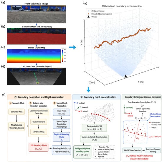
As shown in Figure 6, the proposed method converts the semantic boundary observed in the front-view image into a vehicle-relative distance to the headland [32,33]. The semantic mask contains the land and headland classes shown in Figure 6a,b. Morphological opening and closing are first applied to remove isolated predictions and fill small holes. The interface between the working-farmland and headland regions is then scanned column by column, and the first valid class transition in each image column is retained as a two-dimensional boundary point. Columns without a valid transition are discarded, after which isolated points are removed and one-dimensional smoothing is applied along the horizontal image direction. This procedure yields a continuous image-space boundary while retaining its principal geometric trend.
Figure 6.
Overview of the stereo-vision-based headland boundary reconstruction and distance estimation method: (a) front-view RGB image; (b) semantic segmentation mask and extracted two-dimensional boundary; (c) stereo depth map; (d) reconstructed three-dimensional point cloud of the ground and surrounding objects; (e) retained three-dimensional boundary points; and (f) workflow of boundary extraction, depth association, three-dimensional reconstruction, boundary fitting, and distance estimation.
A ZED 2i stereo camera (Stereolabs Inc., San Francisco, CA, USA) was used with ZED SDK 5.1 at a resolution of 1280 × 720 pixels. The factory-calibrated left-camera raw intrinsics were = 533.675, = 533.740, = 626.545, and = 350.458 pixels, with a stereo baseline of 0.119896 m. Each extracted boundary pixel is associated with the depth provided by the ZED stereo camera and registered to the rectified left image in Figure 6c. Using the calibrated camera intrinsics, the pixel and its depth are back projected to a three-dimensional point. The reconstructed points are subsequently expressed in the ground-related coordinate system through the calibrated camera-to-vehicle transformation. In this coordinate system, denotes the lateral direction, denotes the machinery-forward direction, and ) denotes the ground-plane coordinate of the i-th reconstructed boundary point. Points with missing or invalid depth, or points outside the effective binocular detection region, are rejected. Figure 6d shows the complete reconstructed point cloud containing the ground and surrounding objects, whereas Figure 6e highlights the retained three-dimensional boundary points.
The retained boundary points are projected onto the X-Y ground plane and fitted as a locally linear boundary. The local-line assumption applies only to the boundary segment visible within the effective detection region and does not imply that the entire field boundary is straight. To reduce the effects of segmentation errors and depth outliers, RANSAC is used to identify the boundary inliers, which are subsequently refitted using total least squares. The resulting boundary is represented by Equation (8):
Let denote the camera center in the same ground-plane coordinate system. The vehicle-relative headland distance is calculated as the perpendicular distance from to the fitted boundary at Equation (9):
Rather than reducing the boundary depths to a single statistic, the method reconstructs multiple three-dimensional boundary points, removes inconsistent observations, and estimates the vehicle-relative distance from the fitted spatial boundary. The resulting distance, , is supplied to the distance-threshold-based decision module described in Section 2.4. Because the present system was designed and evaluated for near-perpendicular approaches, is treated as the remaining forward distance.
2.4. Headland Behavioral Decision-Making
A distance-threshold-based behavioral decision method was developed to convert the estimated boundary distance into deceleration and turn-initiation decisions [21]. The method calculates the minimum headland width required for a prescribed turning pattern and determines the distance conditions for maintaining field operation, initiating deceleration, and generating implement-lifting and turn-initiation commands. The detected boundary refers to the field–headland interface.
2.4.1. Headland Width Analysis for Typical Turning Patterns
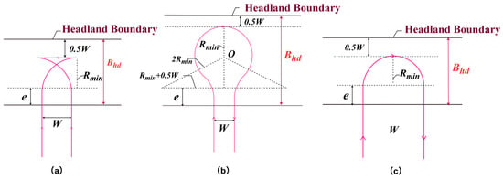
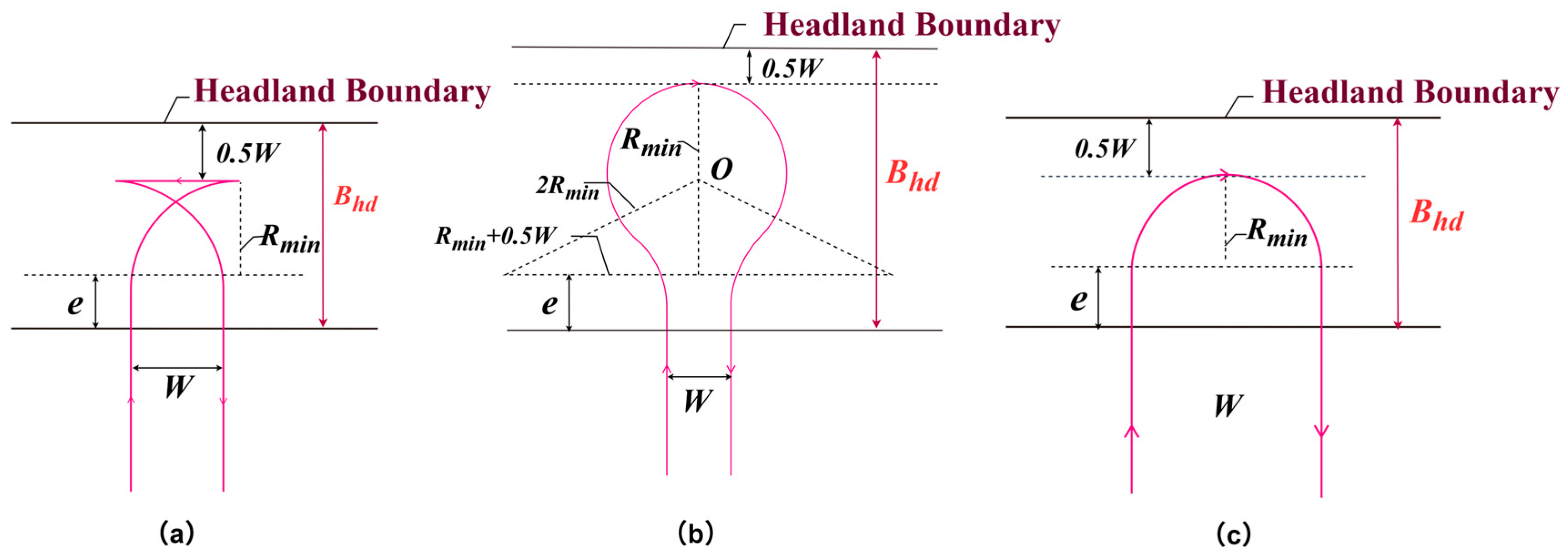
For reciprocating field operations, three representative turning patterns are considered: fishtail, bulb, and semicircular turns, as illustrated in Figure 7. Let denote the minimum turning radius, the working width, and the longitudinal distance from the machine reference point to the rearmost implement–ground contact point. The minimum headland width required for turning pattern is calculated as Equation (10):
Figure 7.
Schematic diagrams of headland width calculations for three turning patterns: (a) fishtail turn; (b) bulb turn; and (c) semicircular turn.
Fishtail and bulb turns are considered when , whereas a semicircular turn is geometrically feasible when .
2.4.2. Distance Threshold-Based Headland Decision-Making
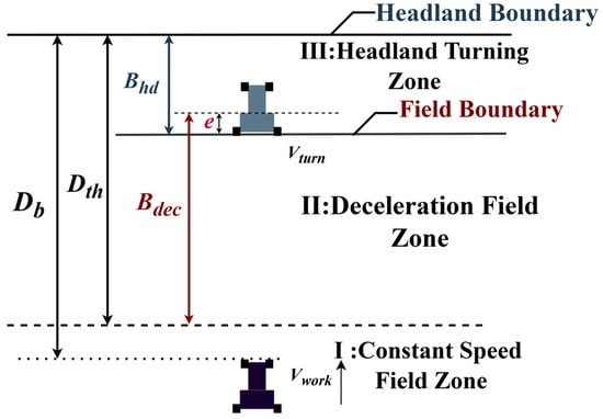
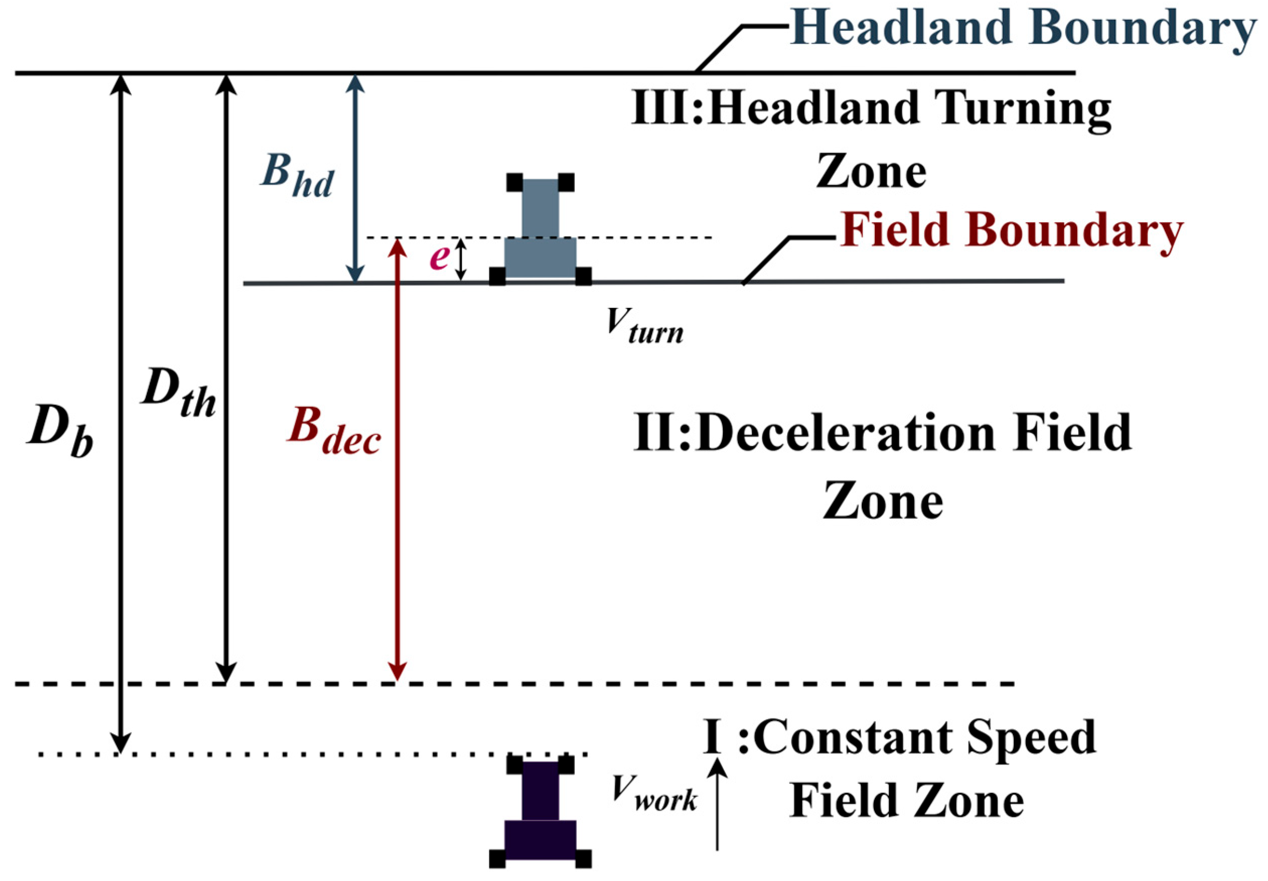
As illustrated in Figure 8, the distance threshold to the headland boundary, , is defined as Equation (11):
where is the required headland width determined by the selected turning pattern and machine implement parameters, and is the longitudinal implement offset defined in Section 2.4.1. The deceleration distance is the vehicle travel distance required to reduce the working speed to the turning speed . Assuming a constant deceleration magnitude > 0, it is calculated as Equation (12):
Figure 8.
Multi-level decision-making framework.
Based on Equations (8)–(12), the measured distance from the agricultural machine to the headland boundary and the distance threshold satisfy the following conditions:
- (1)
- When , the agricultural machine maintains the working speed and continues operation;
- (2)
- When , the agricultural machine begins to decelerate with a deceleration rate ;
- (3)
- When , the agricultural machine is decelerating, with the speed reduced from to ;
- (4)
- When , the agricultural machine lifts the implement and begins executing the selected turn type at speed .
These distance thresholds coordinate deceleration, implement lifting, and turn initiation as the machine approaches the headland.
2.5. Artificial Intelligence (AI) Use Statement
ChatGPT (GPT-5.5) was used only for minor language editing. GPT Image 2 was used to assist in creating selected schematic elements in Figure 5, which were subsequently reviewed and edited by the authors in draw.io. No generative AI tools were used to generate, analyze, or interpret experimental data. The authors take full responsibility for the manuscript.
3. Results
3.1. Evaluation of the Headland Classification Network
To evaluate MobileNetV4-Small as the first-stage classifier in the two-stage framework, 5250 images were used for training, 1500 for validation, and 750 for held-out testing. As shown in Table 1, the test set comprised 500 headland images and 250 field images. MobileNetV4-Small achieved a test accuracy of 97.20%, with macro-averaged precision, recall, and F1-score values of 97.08%, 96.60%, and 96.83%, respectively. Recall for the headland class was 98.40%, with eight headland images misclassified as non-headland, corresponding to a false-negative rate of 1.60%. Conversely, 13 non-headland images were incorrectly classified as headland.
Table 1.
Classification performance of MobileNetV4-Small on the test set.
Under the frame-by-frame classification rule, segmentation is triggered whenever a frame is classified as headland. A false-negative headland prediction therefore prevents segmentation from being triggered for that frame, whereas a false-positive prediction results in an unnecessary segmentation call. The reported false-negative rate characterizes frame-level classification performance and does not quantify the proportion of complete headland-entry events that were missed.
3.2. Evaluation of the Image Segmentation Model
3.2.1. Ablation Study
The segmentation metrics in Table 2, Table 3, Table 4 and Table 5 are reported as the mean (minimum–maximum) across 10 independent training runs. DeepLabV3+ was used as the baseline to evaluate the contributions of Coordinate Attention (CA), Strip Pooling (SP), and Boundary and Dice (B&D) loss. Table 2 presents the segmentation metrics together with the corresponding intervals obtained from independent training runs. Adding CA, SP, and B&D loss individually increased the reported Headland IoU from 89.06% to 91.68%, 91.51%, and 94.06%, respectively. The corresponding Field IoU values increased from 95.02% to 96.13%, 96.50%, and 97.26%. Among the individual modifications, B&D loss produced the largest reported IoU improvement for both classes.
Table 2.
Ablation study results of different modules on Headland and Field classes.
Table 3.
Comparison of different loss functions on Headland and Field classes.
Table 4.
Performance comparison of different models.
Table 5.
Comparative analysis of model pruning and knowledge distillation techniques.
The complete CA-SP-B&D configuration achieved Headland IoU, PA, and Precision values of 94.02%, 96.95%, and 96.89%, respectively, and corresponding Field values of 97.26%, 98.60%, and 98.63%. Compared with B&D loss alone, the complete configuration increased the reported Headland and Field Precision by 0.50 and 0.54 percentage points, respectively. Its Headland IoU was 0.04 percentage points lower, while the reported Field IoU was unchanged. These point estimates indicate a trade-off between precision and region overlap.
3.2.2. Performance Comparison of Loss Functions
Table 3 compares the segmentation results obtained with CE, Boundary, Dice, and B&D losses, including the intervals obtained from independent training runs. B&D loss yielded the highest reported IoU values among the evaluated losses, reaching 94.06% for Headland and 97.26% for Field. These values exceeded those obtained with CE loss by 5.00 and 2.24 percentage points, respectively. B&D loss also achieved the highest reported Precision values, at 96.39% for Headland and 98.09% for Field. These results support the use of combined regional-overlap and boundary supervision for the evaluated headland segmentation task.
3.2.3. Comparison with Classic Semantic Segmentation Models
Under the same dataset partition and training protocol, CA-SP-DeepLabV3+ achieved an mIoU of 95.64%, an mPA of 97.78%, and an Accuracy of 98.09% in Table 4. Compared with the original DeepLabV3+, mIoU increased by 3.60 percentage points, from 92.04% to 95.64%, although model weight increased from 22.4 to 24.1 MB and throughput decreased from 87 to 72 fps. HRNet remained marginally more accurate, exceeding the proposed model by 0.49, 0.28, and 0.21 percentage points in mIoU, mPA, and Accuracy, respectively. However, CA-SP-DeepLabV3+ was 13.4 MB smaller and processed images at 2.12 times the throughput of HRNet. It also exceeded U-Net and PSPNet in all three accuracy metrics while providing more than three times their throughput. The proposed model therefore provided a competitive accuracy efficiency trade-off rather than the highest accuracy on every metric.
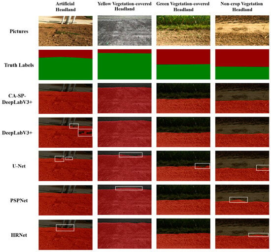
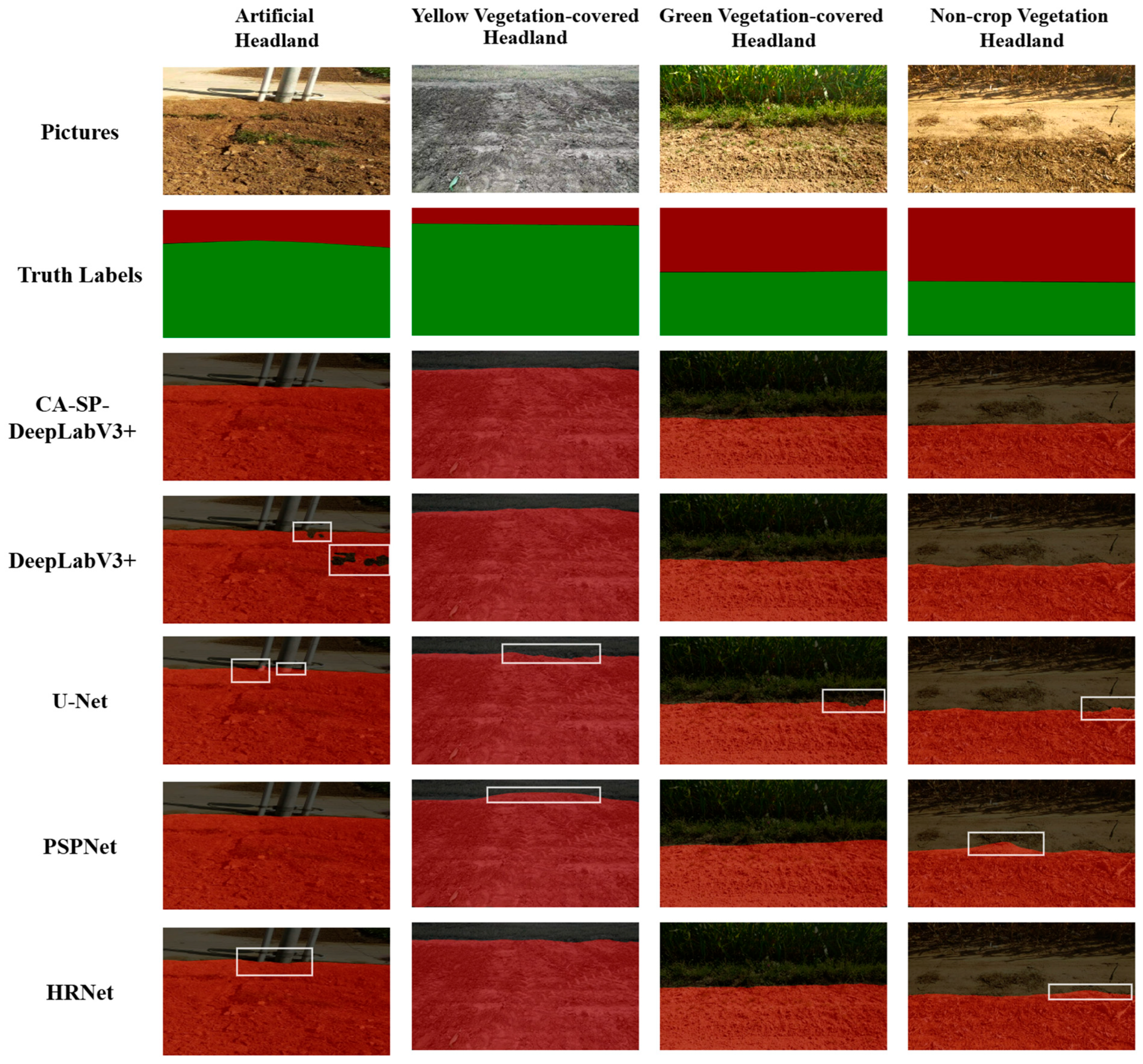
In the representative examples in Figure 9, CA-SP-DeepLabV3+ produced smoother and more continuous boundaries than the comparison models.
Figure 9.
Performance comparison of various models.
3.2.4. Performance Comparison of Model Pruning and Distillation
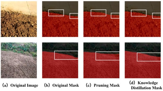
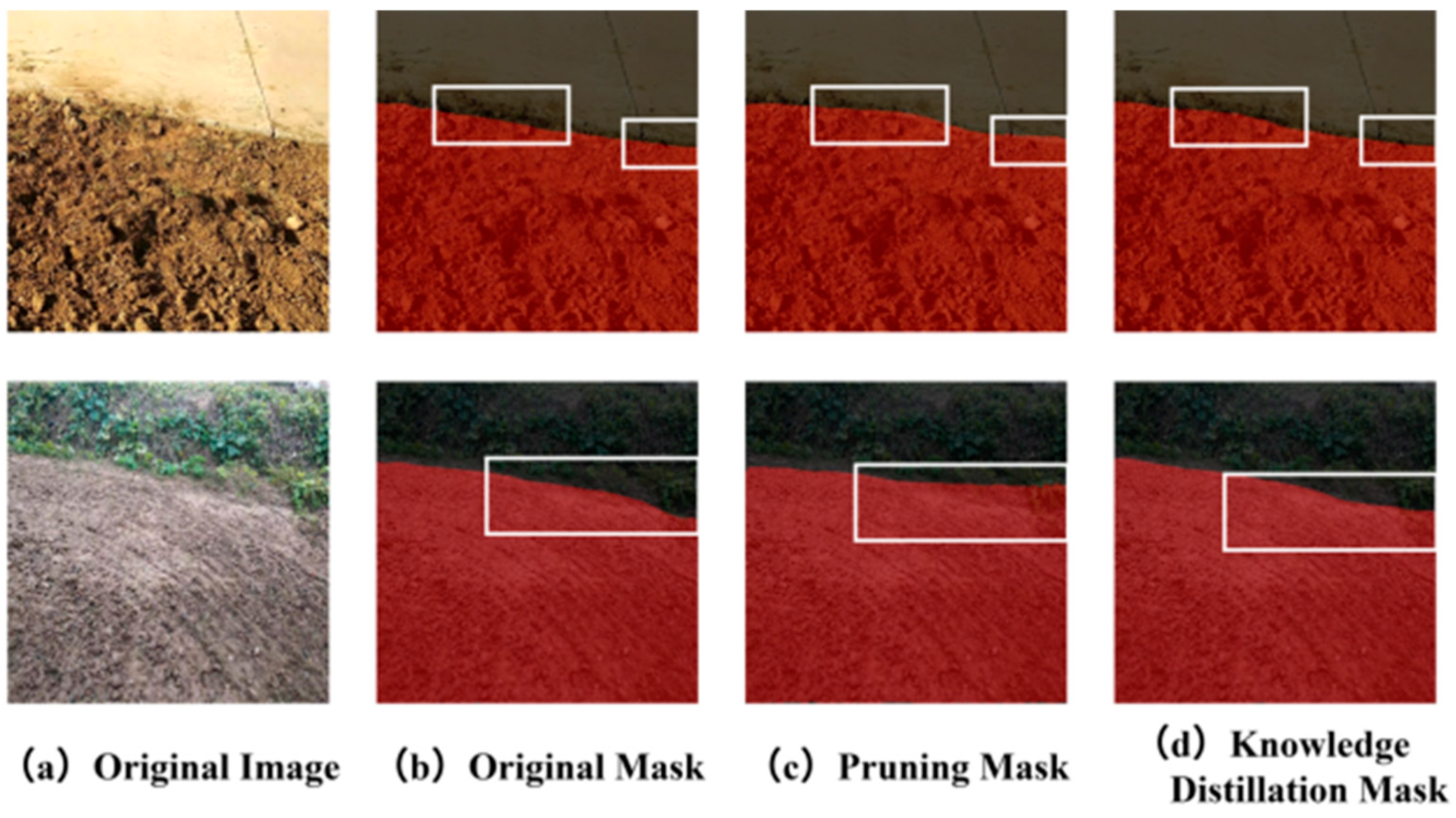
Structured pruning reduced the parameter count from 6.25 M to 4.47 M and FLOPs from 26.72 G to 13.78 G, corresponding to reductions of 28.48% and 48.43%, respectively, in Table 5. Direct pruning decreased the Headland and Field IoU values by 5.50 and 2.56 percentage points. Knowledge distillation subsequently recovered the IoU values to 92.55% and 96.53%, corresponding to recoveries of 4.03 and 1.83 percentage points from the pruning-only results. Residual gaps of 1.47 and 0.73 percentage points remained relative to the unpruned model. These results show that distillation partially recovered the accuracy lost during pruning while retaining the reductions in parameters and FLOPs. Figure 10 shows that distillation visually restored smoother boundary details than pruning alone, consistent with the partial quantitative recovery reported in Table 5.
Figure 10.
Performance comparison between pruning and knowledge distillation.
3.3. Headland Boundary Extraction and Ranging Analysis
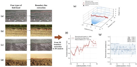
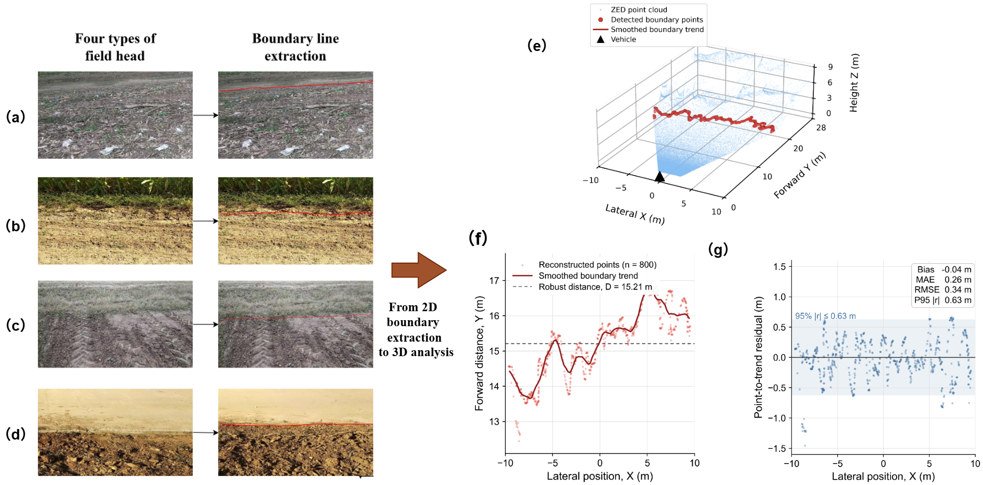
Figure 11 integrates the qualitative boundary extraction results with the quantitative evaluation of three-dimensional reconstruction. In the four representative headland scenes shown in Figure 11a–d, the detected boundary lines followed the visible transition between the cultivated field and the headland under different vegetation and surface conditions. The extracted two-dimensional boundary pixels were subsequently associated with the ZED point cloud to reconstruct the headland boundary relative to the vehicle, as illustrated in Figure 11e. The resulting 800 boundary points formed a continuous three-dimensional profile across the camera field of view. After smoothing the lateral variation in the reconstructed boundary in Figure 11f, the estimated forward distance from the vehicle to the headland boundary was 15.21 m. The point-to-trend residual analysis in Figure 11g yielded a bias of −0.04 m, an MAE of 0.26 m, an RMSE of 0.34 m, and a 95th-percentile absolute residual of 0.63 m. The near-zero bias and the observation that 95% of the absolute residuals did not exceed 0.63 m indicate that most reconstructed points remained close to the smoothed boundary profile. These statistics quantify the internal geometric consistency of the reconstructed boundary.
Figure 11.
Representative headland boundary extraction and three-dimensional reconstruction: (a–d) original images and corresponding boundary extraction results for four representative headland scenes; (e) reconstructed three-dimensional boundary points overlaid on the stereo point cloud; (f) reconstructed boundary points, the smoothed boundary trend, and the estimated vehicle-to-boundary distance; and (g) point-to-trend residuals and summary statistics.
Ranging performance was evaluated under four headland environments at reference distances of 10, 20, and 30 m. Under each condition, the vehicle remained stationary, and ranging outputs were recorded at approximately 20 Hz for approximately 30 s, yielding about 600 samples. Table 6 reports the mean ± standard deviation of valid ranging measurements and the corresponding absolute and relative errors for each condition. The standard deviation describes short term variability within a single acquisition sequence; consecutive samples were not treated as independent experimental repetitions.
Table 6.
Summary of experimental measurement results.
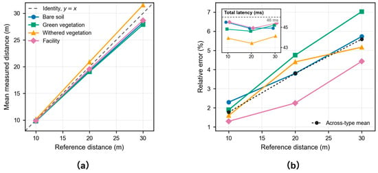
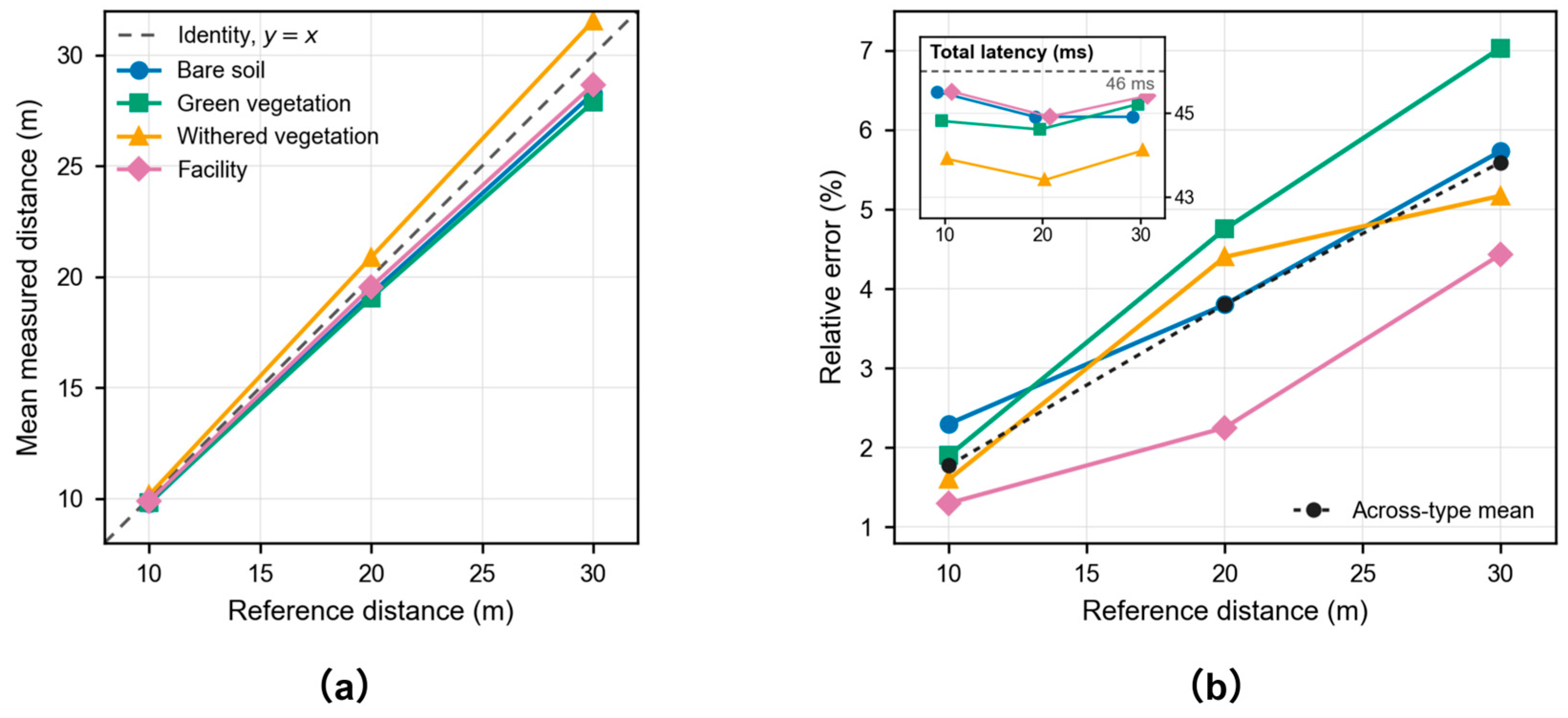
As shown in Figure 12 and summarized in Table 6, the measured distances closely followed the reference distances across the four headland types. The reference distances of 10, 20, and 30 m were determined using GNSS data and tape measurements. The measured distances ranged from 9.77 m to 10.15 m, 19.05 m to 20.88 m, and 27.89 m to 31.55 m, respectively. The corresponding across-type mean relative errors were 1.75%, 3.80%, and 5.59%, respectively, in Figure 12b. Across the individual headland types, the relative errors ranged from 1.30% to 2.30% at 10 m, 2.25% to 4.75% at 20 m, and 4.43% to 7.03% at 30 m. On the NVIDIA Jetson Orin Nano platform, the combined segmentation-inference and ranging latency was 43.4 ms to 45.5 ms across the 12 evaluated conditions, corresponding to an effective processing rate of approximately 22.0 frames s−1 to 23.0 frames s−1.
Figure 12.
Ranging performance under different scenarios: (a) measured versus reference distance; (b) relative error and total latency.
3.4. Headland Turning Decision Test
3.4.1. Headland Turning Width Planning Experiment
Two tractor models and three implements were evaluated to determine the headland widths required for different turning modes. Turn feasibility was first assessed from the machine geometry. Because , semicircular turns were infeasible for the tested machine units. Fishtail turns were also excluded for the 1590 no-till seeder because the towed implement could not reverse during a headland maneuver.
As shown in Table 7, the widths calculated by the proposed method were 8.41% to 15.54% smaller than those reserved by an experienced operator, with a mean reduction of 12.31%. The largest reduction was obtained for the John Deere 904 with the rotary tiller during a fishtail turn. These results demonstrate that the proposed method reduced unnecessary headland occupation while satisfying the geometric constraints of the tested machine units.
Table 7.
Experimental results of headland width comparison.
3.4.2. Motion Planning Experiment Based on Headland Distance
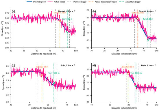
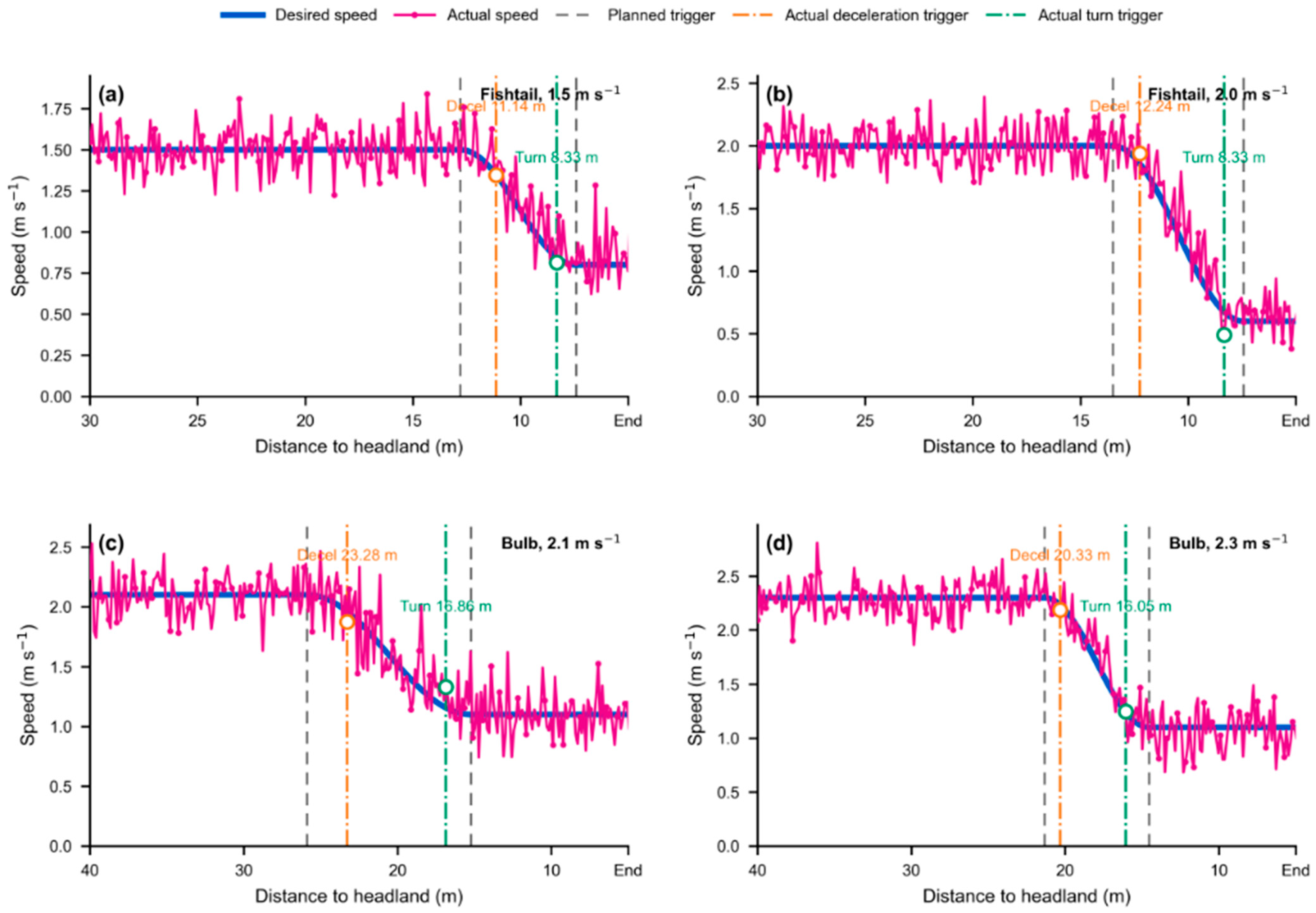
The John Deere 1204 tractor with the rotary tiller was tested under the four operating conditions listed in Table 8. All tests were conducted with the tractor approaching the headland boundary approximately perpendicularly. Consistent with Section 2.3, was therefore treated as the remaining forward distance for the motion decisions. The fishtail tests reduced the working speed from 1.5 to 0.8 m s−1 and from 2.0 to 0.6 m s−1, whereas the bulb-turn tests reduced the speed from 2.1 or 2.3 to 1.1 m s−1. The prescribed deceleration magnitudes were 0.15 or 0.30 m s−2, resulting in deceleration distances of 5.37 m to 10.67 m.
Table 8.
Parameter settings for turning path planning experiment.
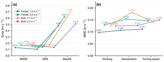
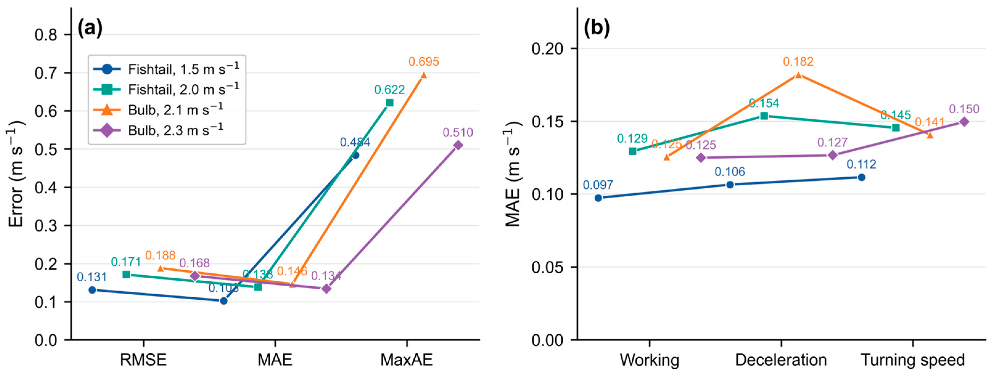
Figure 13a–d shows that the measured speed followed the planned transition through the working-speed, deceleration, and turning-speed stages under all four conditions. The detected deceleration positions were 1.02–2.62 m closer to the headland than the planned triggers. Nevertheless, the command-speed regime was reached 0.90–1.63 m before the required turning-width boundary, indicating that the machine had completed the necessary speed reduction before entering the space-critical turning zone. The quantitative results in Figure 14a show that RMSE, MAE, and MaxAE ranged from 0.131 to 0.188, 0.103 to 0.146, and 0.484 to 0.695 m s−1, respectively. The phase-specific MAE ranged from 0.097 to 0.129 m s−1 during working-speed operation, from 0.106 to 0.182 m s−1 during deceleration, and from 0.112 to 0.150 m s−1 during turning-speed operation in Figure 14b. The 2.1 m s−1 bulb-turn condition produced the largest overall and deceleration stage errors, consistent with its greater transient speed fluctuations. Each condition contained 300 paired desired- and measured-speed samples.
Figure 13.
Headland distance-based speed tracking and trigger responses under four operating conditions: (a) fishtail turn at 1.5 m s−1; (b) fishtail turn at 2.0 m s−1; (c) bulb turn at 2.1 m s−1; (d) bulb turn at 2.3 m s−1.
Figure 14.
Speed-tracking errors under four headland-turning conditions: (a) overall RMSE, MAE, and MaxAE; (b) MAE during the working, deceleration, and turning-speed stages.
Overall, Table 7 and Table 8 together with Figure 14 demonstrate that the proposed distance-based decision strategy reduced headland occupation and achieved stable turn speed regulation under the four tested conditions. These results validate the headland decision and longitudinal speed-control performance.
4. Discussion
4.1. Boundary-Aware Segmentation and Lightweight Deployment
Liu et al. [23] combined lightweight feature extraction, attention mechanisms, and strip pooling to improve semantic segmentation. Our results similarly indicate the usefulness of these components, although their contributions differed in the headland task. Boundary–Dice supervision produced the largest individual improvement in headland IoU, suggesting that boundary-specific supervision was particularly important under the evaluated conditions.
The CA, SP, and B&D loss components improved the model’s ability to distinguish the narrow and irregular boundary between the cropped field and the headland. In particular, the B&D loss increased the headland IoU from 89.06% to 94.06% compared with cross-entropy loss, indicating that joint region and boundary constraints were more appropriate for this boundary-sensitive task. The complete CA-SP-DeepLabV3+ model achieved an mIoU of 95.64%, an accuracy of 98.09%, and a processing speed of 72 fps. Although HRNet produced slightly higher mIoU and accuracy values, the proposed model operated at more than twice its speed and required a smaller model size. After pruning and knowledge distillation, the parameter count and FLOPs were reduced by 28.48% and 48.43%, respectively, while the headland and field IoUs remained at 92.55% and 96.53%. These results demonstrate a favorable balance between boundary-recognition performance and computational efficiency for embedded agricultural platforms.
4.2. Contribution of Binocular Ranging to Decision Reliability
Liu et al. [11] reported mean relative ranging errors of 6.72%, 4.80%, and 4.35% at 25, 20, and 15 m, respectively. Our results showed the same trend of decreasing error at shorter distances, with relative errors of 4.43–7.03% at 30 m and 1.30–2.30% at 10 m. At the shared distance of 20 m, our across-type mean relative error was 3.80%, compared with their reported 4.80%. However, differences in scene composition, camera configuration, and evaluation procedures prevent attributing this numerical difference solely to the proposed method. This improvement in accuracy is beneficial because the final turning decision requires more precise distance information near the boundary. However, larger errors at 20 m to 30 m may affect the initial deceleration trigger because several planned trigger positions fell within this range. Therefore, the ranging results support the feasibility of distance-based decision-making but also suggest that ranging uncertainty should be considered when defining the deceleration threshold.
4.3. Spatial Efficiency and Timing of the Turning Decision
The geometry-based planning method reduced the reserved headland width by 8.41% to 15.54% compared with experienced-operator practice, with an average reduction of 12.31%. This indicates that configuration-specific planning can avoid excessive land reservation while excluding turning modes that are incompatible with the machine geometry or implement characteristics. In the four motion experiments, the detected deceleration onset occurred 1.02 m to 2.62 m later than the planned trigger. Nevertheless, the tractor reached the turn-speed regime 0.90 m to 1.63 m before the corresponding turning-width boundary. Together with the overall speed-tracking RMSE of 0.131–0.188 m s−1, these results show that the proposed decision logic coordinated the measured headland distance with the required speed transition under the tested conditions. The observed deceleration delays may reflect the combined effects of ranging uncertainty, processing and control latency, and vehicle dynamic response. At 30 m, the absolute errors of the mean distance estimates ranged from 1.33 to 2.11 m, indicating that long-range ranging errors could materially influence trigger timing. In particular, overestimating the remaining distance can delay deceleration, whereas underestimating it can cause earlier triggering. However, the ranging and motion-test results do not establish a direct causal relationship between individual ranging errors and the observed trigger offsets. At the maximum tested working speed of 2.3 m s−1, the reported visual processing latency of less than 46 ms corresponds to less than 0.11 m of vehicle travel. This processing delay alone is therefore insufficient to explain the observed offsets of 1.02–2.62 m. Additional contributions may arise from communication and control delays, actuator response, and variations in the achieved deceleration. He et al. [17] reduced turning-path length and completion time through dynamic headland path planning. Our results complement this work by showing how perceived boundary distance can support deceleration before entering the required turning space. The observed headland-width reduction concerns spatial reservation and should not be interpreted as an equivalent reduction in turning-path length or completion time.
A possible extension is to increase the nominal deceleration trigger distance by a safety margin that accounts for distance overestimation, travel during the total system delay, and additional distance required when the achieved deceleration is lower than prescribed. Such a margin should be determined from repeated, synchronized ranging and vehicle-response measurements and validated under different operating conditions.
4.4. Limitations and Future Development
The present experiments were conducted at the same experimental site and covered four representative headland environments. Motion-decision performance was evaluated only under the conventional operating scenario in which the tractor approached the headland boundary perpendicularly. Consequently, the current results validate headland perception, distance-triggered decision timing, and longitudinal speed regulation. Future work should incorporate safety margins that account for ranging uncertainty and conduct broader field experiments.
5. Conclusions
This study developed a vision-based framework linking headland-boundary perception and stereo ranging with distance-triggered behavioral decisions. The framework combines boundary distance with tractor–implement geometry and operating conditions to determine the required headland width and the timing of deceleration and turn preparation.
Under the tested conditions, the planned headland widths were 8.41% to 15.54% smaller than those reserved by an experienced operator. The tractor reached the prescribed turning-speed regime before entering the required turning space in all four evaluated operating conditions. These findings support the practical use of boundary-distance estimates to coordinate speed reduction with machine-specific turning requirements.
The framework provides decision-level inputs for subsequent implement and steering control, with potential applications in automated headland operations on tractors, harvesters, and rice transplanters. Deployment on different machines would require machine-specific calibration of camera installation, vehicle–implement geometry, and deceleration parameters. Under actual field conditions, sensor noise, vehicle vibration, illumination changes, and partial occlusion may affect boundary segmentation and stereo depth estimation, introducing uncertainty into distance-triggered decisions. Future work should evaluate these effects across machines, sites, and operating conditions and investigate the integration of visual perception with Global Navigation Satellite System (GNSS) positioning and inertial measurements. Such integration could provide complementary position and attitude information to support more consistent decision-making when visual observations are degraded. Its benefits for robustness and decision reliability remain to be experimentally validated.
Author Contributions
Conceptualization, J.W.; methodology, J.W. and H.L.; software, J.W.; validation, Z.M.; formal analysis, X.C.; investigation, J.W.; resources, Z.M.; data curation, X.Z.; writing—original draft preparation, J.W.; writing—review and editing, H.L.; supervision, H.L.; funding acquisition, H.L. All authors have read and agreed to the published version of the manuscript.
Funding
This research was funded by the National Agricultural Science and Technology Major Project of China (1601).
Institutional Review Board Statement
Not applicable; this study did not involve humans or animals.
Informed Consent Statement
Not applicable.
Data Availability Statement
The original contributions presented in this study are included in the article. Further inquiries can be directed to the corresponding author.
Acknowledgments
During the preparation of this manuscript, the authors used ChatGPT (GPT-5.5; OpenAI, San Francisco, CA, USA) for English language polishing. The authors reviewed and edited all outputs and take full responsibility for the content of this publication.
Conflicts of Interest
The authors declare no conflicts of interest.
Abbreviations
The following abbreviations are used in this manuscript:
| 3D | Three-Dimensional |
| ASPP | Atrous Spatial Pyramid Pooling |
| B&D | Boundary and Dice Loss |
| CA | Coordinate Attention |
| CE | Cross-Entropy |
| CPU | Central Processing Unit |
| FLOPs | Floating-Point Operations |
| FN | False Negative |
| FP | False Positive |
| fps | Frames per Second |
| GNSS | Global Navigation Satellite System |
| GPU | Graphics Processing Unit |
| HRNet | High-Resolution Network |
| IoU | Intersection over Union |
| MAE | Mean Absolute Error |
| mIoU | Mean Intersection over Union |
| mPA | Mean Pixel Accuracy |
| PA | Pixel Accuracy |
| RANSAC | Random Sample Consensus |
| RGB-D | Red–Green–Blue and Depth |
| RMSE | Root Mean Square Error |
| SGD | Stochastic Gradient Descent |
| SP | Strip Pooling |
| TN | True Negative |
| TP | True Positive |
References
- Hossain, M.S.; Rahman, M.; Rahman, A.; Kabir, M.M.; Mridha, M.F.; Huang, J.; Shin, J. Automatic navigation and self-driving technology in agricultural machinery: A state-of-the-art systematic review. IEEE Access 2025, 13, 94370–94401. [Google Scholar] [CrossRef] [Scilit]
- Meng, Z.; Wang, H.; Fu, W.; Liu, M.; Yin, Y.; Zhao, C. Research status and prospects of agricultural machinery autonomous driving. Trans. Chin. Soc. Agric. Mach. 2023, 54, 1–16. (In Chinese) [Google Scholar] [CrossRef]
- Yang, X.; Zhong, J.; Lin, K.; Wu, J.; Chen, J.; Si, H. Research progress on binocular stereo vision technology and its applications in smart agriculture. Trans. Chin. Soc. Agric. Eng. 2025, 41, 27–39. (In Chinese) [Google Scholar] [CrossRef]
- Chen, Y.; Zhang, M.; Ma, W.; Liu, Z.; Ji, Y. Positioning method of integrated navigation based on GPS and machine vision. Trans. Chin. Soc. Agric. Eng. 2011, 27, 126–130. (In Chinese) [Google Scholar] [CrossRef]
- Ren, Y.; Zhang, B.; Li, Y.; Chen, C.; Li, W.; Ma, Y. Computer vision-based steering path visualization of headlands in soybean fields. Front. Plant Sci. 2025, 16, 1673567. [Google Scholar] [CrossRef] [Scilit] [PubMed]
- Huang, P.; Zhu, L.; Zhang, Z.; Yang, C. Row end detection and headland turning control for an autonomous banana-picking robot. Machines 2021, 9, 103. [Google Scholar] [CrossRef] [Scilit]
- Li, J.; Chen, B.; Liu, Y.; Zha, T. Detection for navigation route for cotton harvester based on machine vision. Trans. Chin. Soc. Agric. Eng. 2013, 29, 11–19. (In Chinese) [Google Scholar]
- Wang, Q.; Liu, H.; Yang, P.; Meng, Z. Detection method of headland boundary line based on machine vision. Trans. Chin. Soc. Agric. Mach. 2020, 51, 18–25. (In Chinese) [Google Scholar] [CrossRef]
- Qiao, Y.; Peng, S.; Meng, Z.; Wang, Q.; Liu, S. Detection system of headland boundary line based on machine vision. J. Agric. Mech. Res. 2022, 44, 24–30. (In Chinese) [Google Scholar] [CrossRef]
- Qiao, Y.; Liu, H.; Meng, Z.; Chen, J.; Ma, L. Method for the automatic recognition of cropland headland images based on deep learning. Int. J. Agric. Biol. Eng. 2023, 16, 216–224. [Google Scholar] [CrossRef] [Scilit]
- Liu, H.; Li, K.; Ma, L.; Meng, Z. Headland identification and ranging method for autonomous agricultural machines. Agriculture 2024, 14, 243. [Google Scholar] [CrossRef] [Scilit]
- He, Y.; Zhang, X.; Zhang, Z.; Fang, H. Automated detection of boundary line in paddy field using MobileV2-UNet and RANSAC. Comput. Electron. Agric. 2022, 194, 106697. [Google Scholar] [CrossRef] [Scilit]
- Ji, J.; Han, Z.; Zhao, K.; Li, Q.; Du, S. Detection of the farmland plow areas using RGB-D images with an improved YOLOv5 model. Int. J. Agric. Biol. Eng. 2024, 17, 156–165. [Google Scholar] [CrossRef] [Scilit]
- Li, D.; Li, B.; Long, S.; Feng, H.; Wang, Y.; Wang, J. Robust detection of headland boundary in paddy fields from continuous RGB-D images using hybrid deep neural networks. Comput. Electron. Agric. 2023, 207, 107713. [Google Scholar] [CrossRef] [Scilit]
- Liu, G.; Jin, C.; Ni, Y.; Yang, T.; Liu, Z. UCIW-YOLO: Multi-category and high-precision obstacle detection model for agricultural machinery in unstructured farmland environments. Expert Syst. Appl. 2025, 294, 128686. [Google Scholar] [CrossRef] [Scilit]
- Soitinaho, R.; Väyrynen, V.; Oksanen, T. Heuristic cooperative coverage path planning for multiple autonomous agricultural field machines performing sequentially dependent tasks of different working widths and turn characteristics. Biosyst. Eng. 2024, 242, 16–28. [Google Scholar] [CrossRef] [Scilit]
- He, Z.; Bao, Y.; Yu, Q.; Lu, P.; He, Y.; Liu, Y. Dynamic path planning method for headland turning of unmanned agricultural vehicles. Comput. Electron. Agric. 2023, 206, 107699. [Google Scholar] [CrossRef] [Scilit]
- Wu, T.; Guo, H.; Zhou, W.; Gao, G.; Wang, X.; Yang, C. Navigation path extraction for farmland headlands via red-green-blue and depth multimodal fusion based on an improved DeepLabV3+ model. Eng. Appl. Artif. Intell. 2025, 151, 110681. [Google Scholar] [CrossRef] [Scilit]
- Liu, Z.; Wu, X.; Gao, W.; Ning, F.; Zhang, W.; He, J.; Liu, M.; Chen, X.; Fang, P. Research on a vision navigation system for rice transplanters based on machine vision fused with GNSS. Biosyst. Eng. 2026, 262, 104354. [Google Scholar] [CrossRef] [Scilit]
- Backman, J.; Piirainen, P.; Oksanen, T. Smooth turning path generation for agricultural vehicles in headlands. Biosyst. Eng. 2015, 139, 76–86. [Google Scholar] [CrossRef] [Scilit]
- Chen, T.; Xu, L.; Ahn, H.S.; Lu, E.; Liu, Y.; Xu, R. Evaluation of headland turning types of adjacent parallel paths for combine harvesters. Biosyst. Eng. 2023, 233, 93–113. [Google Scholar] [CrossRef] [Scilit]
- Qin, D.; Leichner, C.; Delakis, M.; Fornoni, M.; Luo, S.; Yang, F.; Wang, W.; Helwegen, B.; Gunawan, R.; Howard, A. MobileNetV4: Universal models for the mobile ecosystem. arXiv 2024, arXiv:2404.10518. [Google Scholar] [CrossRef] [Scilit]
- Liu, Y.; Bai, X.; Wang, J.; Li, G.; Li, J.; Lv, Z. Image semantic segmentation approach based on DeepLabV3 plus network with an attention mechanism. Eng. Appl. Artif. Intell. 2024, 127, 107260. [Google Scholar] [CrossRef] [Scilit]
- Yu, H.; Luo, Q.; Peng, W.; Zheng, L.; Ju, J.; Zhuo, H. PKD-YOLOv8: A collaborative pruning and knowledge distillation framework for lightweight rapeseed pest detection. Sensors 2025, 25, 5004. [Google Scholar] [CrossRef] [Scilit] [PubMed]
- Yang, T.; Zhou, S.; Xu, A.; Ye, J.; Yin, J. An approach for plant leaf image segmentation based on YOLOv8 and the improved DeepLabV3+. Plants 2023, 12, 3438. [Google Scholar] [CrossRef] [Scilit] [PubMed]
- Chi, Y.; Li, L.; Wang, J.; Sun, Y. Enhanced lane detection via connectivity and boundary refinement for real-time applications. Vis. Comput. 2025, 41, 10873–10882. [Google Scholar] [CrossRef] [Scilit]
- Kervadec, H.; Bouchtiba, J.; Desrosiers, C.; Granger, E.; Dolz, J.; Ben Ayed, I. Boundary loss for highly unbalanced segmentation. Med. Image Anal. 2021, 67, 101851. [Google Scholar] [CrossRef] [Scilit] [PubMed]
- Sudre, C.H.; Li, W.; Vercauteren, T.; Ourselin, S.; Jorge Cardoso, M. Generalised dice overlap as a deep learning loss function for highly unbalanced segmentations. In Deep Learning in Medical Image Analysis and Multimodal Learning for Clinical Decision Support; Cardoso, M.J., Arbel, T., Carneiro, G., Syeda-Mahmood, T., Tavares, J.M.R.S., Moradi, M., Bradley, A., Greenspan, H., Papa, J.P., Madabhushi, A., et al., Eds.; Springer International Publishing: Cham, Switzerland, 2017; Volume 10553, pp. 240–248. [Google Scholar] [CrossRef] [Scilit] [PubMed]
- Zhao, H.; Shi, J.; Qi, X.; Wang, X.; Jia, J. Pyramid scene parsing network. In Proceedings of the 2017 IEEE Conference on Computer Vision and Pattern Recognition (CVPR), Honolulu, HI, USA, 21–26 July 2017; pp. 6230–6239. [Google Scholar] [CrossRef] [Scilit]
- Wang, J.; Sun, K.; Cheng, T.; Jiang, B.; Deng, C.; Zhao, Y.; Liu, D.; Mu, Y.; Tan, M.; Wang, X.; et al. Deep high-resolution representation learning for visual recognition. IEEE Trans. Pattern Anal. Mach. Intell. 2021, 43, 3349–3364. [Google Scholar] [CrossRef] [Scilit] [PubMed]
- Chang, Z.; Li, H.; Chen, D.; Liu, Y.; Zou, C.; Chen, J.; Han, W.; Liu, S.; Zhang, N. Crop type identification using high-resolution remote sensing images based on an improved DeepLabV3+ network. Remote Sens. 2023, 15, 5088. [Google Scholar] [CrossRef] [Scilit]
- Kim, W.-S.; Lee, D.-H.; Kim, Y.-J.; Kim, T.; Lee, W.-S.; Choi, C.-H. Stereo-vision-based crop height estimation for agricultural robots. Comput. Electron. Agric. 2021, 181, 105937. [Google Scholar] [CrossRef] [Scilit]
- Yun, C.; Kim, H.-J.; Jeon, C.-W.; Gang, M.; Lee, W.S.; Han, J.G. Stereovision-based ridge-furrow detection and tracking for auto-guided cultivator. Comput. Electron. Agric. 2021, 191, 106490. [Google Scholar] [CrossRef] [Scilit]

Disclaimer/Publisher’s Note: The statements, opinions and data contained in all publications are solely those of the individual author(s) and contributor(s) and not of MDPI and/or the editor(s). MDPI and/or the editor(s) disclaim responsibility for any injury to people or property resulting from any ideas, methods, instructions or products referred to in the content. |
© 2026 by the authors. Licensee MDPI, Basel, Switzerland. This article is an open access article distributed under the terms and conditions of the Creative Commons Attribution (CC BY) license.