Research on Local Operation Path Planning of Paddy Field Land Leveler Based on the Improved Dung Beetle Optimizer Algorithm

Abstract

Regarding the path planning problem for the local leveling operation of the land leveler, this paper proposes a path planning method based on the improved dung beetle optimizer (IDBO) algorithm. Firstly, a comprehensive evaluation objective function was established for the local operation path planning of the land leveler, which included the path length, under-excavation amount, under-filling amount, as well as the total amount of excavated and filled soil. Then, IDBO algorithm was constructed, an initialization population strategy based on Fuch chaotic mapping and reverse learning strategy was designed, as well as an improved ball-rolling behavior that integrates the search strategy of the Aquila high soar with the vertical stoop from the Aquila optimizer algorithm. Test functions were used to verify the superiority of the IDBO algorithm compared to the dung beetle optimizer (DBO) algorithm, the particle swarm optimization (PSO) algorithm and the gray wolf optimizer (GWO) algorithm. Finally, taking the paddy fields in a real environment as the object, a hardware platform for data acquisition was constructed, and data collection, analysis, terrain modeling, and path planning experiments were carried out with paddy fields in the natural environment as the measured objects. The experimental results show that, for the primary optimization objective of load variation cost, as well as path length cost, compared with the other three algorithms (PSO, GWO, DBO), the IDBO algorithm achieved improvements of 7.0%, 12.3%, and 6.6% on Plot 1, 1.6%, 9.2%, and 1.6% on Plot 2, 4.0%, 6.1%, and 1.5% on Plot 3, and 3.3%, 24.1%, and 3.4% on Plot 4.

1. Introduction

The continued growth of the global population, rising incomes, and the expanding use of bio-fuels are exerting unprecedented pressure and challenges on global agriculture and natural resources. Meanwhile, agricultural production practices are having a significant impact on biodiversity, greenhouse gas concentrations, and water and land resources. As a result, agriculture is confronted with the dual challenge of meeting the ever-increasing demand for food while reducing environmental damage [1]. Traditional manual land leveling relies on the operator’s experience, which often leads to poor leveling quality, low coverage, and repetitive leveling. Far, S.T. et al. [2] sampled 151 experts from Fars Province, Iran, and the results showed that the experts considered uniform irrigation, conservation tillage, and reduced water consumption to be the aspects of current leveling technology that most influence agricultural production. To improve irrigation efficiency, crop seeding uniformity, and crop yield, developing precision agriculture is a classic pathway that can promote the sustainability of agricultural production and maximize agricultural productivity in multiple respects, with land leveling being the primary step [3,4]. Field experiments conducted by Sarfraz Hashim et al. in Pakistan and China demonstrated that precision laser land leveling (LLL) technology significantly reduces farmland irrigation water consumption, improves irrigation efficiency, and increases wheat yield [5]. Oztekin, T. et al. [6] studied the effects of land leveling on soil bulk density and field capacity at different soil layers and concluded that although land leveling is an agricultural practice that helps distribute irrigation water uniformly, unreasonable leveling methods and poor leveling results can cause significant changes in soil properties and may even produce adverse effects shortly after the leveling operation.

Therefore, research on automatic navigation technology for farmland leveling is an important component of the development of precision agriculture. Path planning technology, as a key part of the automatic navigation technology for agricultural land levelers, can effectively guide the leveler in transporting and placing earthwork in a rational manner, thus completing the leveling operation scientifically and efficiently [7,8].

Currently, genetic algorithm (GA), particle swarm optimization (PSO) algorithm, A* algorithm (A*) and artificial potential field (APF) method are all commonly used algorithms in path planning problems. However, unlike conventional path planning, the path planning of land leveler involves earth excavation and filling as well as elevation changes. When planning the route, not only should the shortest path be the optimization goal, but also the efficiency of earthwork excavation and filling as well as the quality of the leveling land should be taken into consideration [9,10].

The path planning for ground operations is generally divided into global operation path planning and local operation path planning. Global leveling operation path planning generates a coverage path that traverses the entire field, whereas local leveling operation path planning generates a local path between two task points that does not cover the entire field. The objective is to reduce the elevation difference between the high and low points in locally undulating areas, so as to plan a local leveling operation path that can maximize the efficiency of excavation and filling. The objective of the global operation path planning is to reduce the overall changing trend of the farmland and improve the overall flatness of the farmland. Liu Gang et al. [11] proposed a global path planning method applicable to GNSS-based farmland leveling operations, aiming to enhance the efficiency of soil excavation and filling. They integrated K-means clustering for farmland and generated a planar path that traverses the entire farmland. Wang Tingting [12] proposed an automatic path planning method, established a three-dimensional farmland terrain model, introduced a leveling shovel capacity threshold, and generated a path covering the entire field based on the principle that the current soil volume in the leveling shovel during operation should be as close as possible to the maximum capacity. Xi Xiaobo et al. [13] proposed a dynamic expansion neighborhood path planning method. Based on the three-dimensional terrain model of farmland, a neighborhood matrix was introduced, and by continuously expanding the neighborhood matrix, a planning path covering all the farmland was generated. The path of the global operation planning is relatively long and covers the entire field. It is usually a combination of multiple different paths. However, when the leveling machine performs flatting operations according to the global operation planning path, some problems are inevitable. For example, during the leveling process, the leveling shovel may shovel too much soil, causing overloading. And after the leveling, some local areas still do not meet the requirements. Therefore, combining the global operation path planning and the local operation path planning will be one of the main research directions of the agricultural land leveling navigation technology.

Research on the path planning problem for local leveling operations of land leveler. Jing Yunpeng et al. [14] proposed a three-dimensional path planning method for farmland leveling based on the improved ant colony optimization (ACO) algorithm. By improving the state transition probability function and the adaptive pheromone evaporation coefficient, compared with the planning path and generation time obtained by the original ACO, the proposed method has shorter planning time and better path planning effect. Chen Wenming et al. [15] proposed a farmland leveling path planning method based on a variable scale distribution strategy and an improved ant colony algorithm. By constructing a farmland terrain elevation difference model, setting nodes at different scales, and adopting a rolling optimization approach, the proposed method realizes whole-field leveling path planning and substantially improves the efficiency of land leveling operations. The path planning for local operations mainly serves two purposes: (1) Before the land leveler performs global leveling operations, there are areas in the field where the terrain is excessively high and areas where it is excessively low. Local operation path planning is carried out first to transport soil from the high areas to the low areas, thereby reducing the overall terrain variation in the field and improving the leveling quality of the subsequent global operation. (2) After the land leveler completes the leveling operation according to the globally planned path, although the overall terrain has become smoother, there may still be some areas where the local flatness does not comply with the requirements. These areas can be leveled through local operation path planning.

To achieve local operation path planning, this paper constructs a path planning objective function model for the land leveler and proposes a land leveling path planning method based on the improved dung beetle optimizer algorithm, which is used to guide the land leveler to perform local leveling operation. Compared with classic algorithms such as GA, PSO and ACO, the DBO algorithm has better advantages in terms of global search ability, the ability to emerge from local optima and convergence speed. It has been applied in the field of path planning at present. Hongmei Fei et al. [16] proposed a multi-strategy DBO algorithm based on the combination of Latin hypercube sampling, golden sine function and adaptive weights for 3D path planning of unmanned aerial vehicles. Lixing Liu et al. [17] proposed a coverage path planning method for orchard lawn mowers based on the DBO algorithm. However, relatively few scholars have applied the DBO algorithm to the research on the operation path planning of land leveler. Based on the traditional dung beetle algorithm, this paper designs the IDBO algorithm, introducing the Fuch chaotic mapping and reverse learning mechanism into the population generation strategy to improve the distribution balance and diversity of the initial population. The search strategy of the Aquila high soar with the vertical stoop in the Aquila optimizer algorithm is integrated into the ball-rolling behavior of the DBO algorithm to expand the search range of the algorithm. The IDBO algorithm is applied to the path planning research for the local operation of the agricultural land leveler, achieving good results.

2. Problem Description

The land leveler performs leveling operations in the field through a leveling shovel attached to the tractor. The leveling shovel is maintained at a set reference elevation, excavating soil when passing through areas above the reference elevation and filling soil when passing through areas below it. Based on the operational characteristics of the land leveler, the research on the path planning for local leveling of farmland mainly focuses on several key indicators such as the efficiency of earthwork excavation and filling, the quality of land leveling, and the length of the operation path. The aim is to find a path that, under the movement limitations of the land leveler, can achieve the maximum amount of earthwork excavation and filling, while also providing good land leveling quality and having a shorter travel distance. Based on the above objectives, this paper constructs a comprehensive evaluation function that incorporates path length, under-excavation and under-filling amount, load variation in the leveling shovel, and mechanical kinematic constraints. Let $X$ be the set of key points of the path generated by the optimization algorithm, and the total evaluation function $F\left(X\right)$ is shown as Equation (1):

$$\begin{array}{c}F\left(X\right)=min({\omega }_1{f}_{dist}+{\omega }_2{f}_{cut}+{\omega }_3{f}_{fill}+{\omega }_4{f}_p)\end{array}$$

(1)

In the equation,

$f_{dist}$ reflects the fuel consumption and time cost of the operation, with the unit of m. The land leveler should select a path as short as possible, but the path length should not be excessively shortened at the expense of operation quality.

$f_{cut}$ represents the amount of soil that is not excavated due to the capacity limitation of the leveling shovel, which affects the leveling quality, with the unit of m³. Under-excavation causes the high-terrain areas to remain above the reference elevation.

$f_{fill}$ represents the amount of soil that is not filled because the soil already loaded in the leveling shovel cannot completely fill the target area, which affects the leveling quality, with the unit of m³. Under-filling causes the low-terrain areas to remain below the reference elevation.

$f_p$ characterizes the effective operation state of the leveling shovel during the leveling process. The closer the leveling shovel operates to its full-load state, the higher the operation efficiency.

${\omega }_1,{\omega }_2,{\omega }_3,{\omega }_4$ are the weighting coefficients for the path length cost, under-excavation cost, under-filling cost, and leveling shovel load variation cost, respectively. The weighting coefficients satisfy ${\omega }_4\gg {\omega }_3={\omega }_2\gg {\omega }_1$ thereby reflecting the priority requirement of the local operation path planning: effective operation amount > leveling quality > energy consumption.

The specific meanings and mathematical models of each cost function are shown as follows:

2.1. Path Length Cost Function $f_{dist}$

The path length determines the travel time and fuel consumption for land leveling operations. By interpolation, the path is discretized into a sequence of $N$ key points $P=\left\{\right(x_i,y_i\left)\right|i=1,2,\dots ,N\}$, The total path length cost function $f_{dist}$ is shown as Equation (2):

$$\begin{array}{c}{f}_{dist}={\displaystyle \sum _{i=1}^{N-1}} \sqrt{(x_{i+1}-x_i{)}^2+(y_{i+1}-y_i{)}^2}\end{array}$$

(2)

$$min\left(R_{(i,i+1)}\right)<R_{min }$$

(3)

To ensure that the generated path meets the steering requirements for the land leveling operation, a minimum turning radius constraint is introduced as Equation (3). Where $R_{(i,i+1)}$ represents the turning radius between the key path points i and i + 1 on the planned path, $R_{min}$ represents the minimum turning radius allowed by the land leveler.

2.2. Under-Excavation Cost Function $f_{cut}$

The under-excavation cost reflects the amount of excavation work that the land leveler is unable to complete when passing through areas with high terrain, because the amount of earth to be excavated exceeds the capacity of the leveling shovel. Let the theoretical amount of earth to be excavated for the $i$-th section be $V_{cut}^{\left(i\right)}$, the maximum capacity of the leveling shovel be $V_{max}$, and the current loaded earth amount be $L_{current}$. Under-excavation amount for this section $\Delta f_{cut}^{\left(i\right)}$ is shown as Equation (4):

$$\begin{array}{c}\Delta f_{cut}^{\left(i\right)}=max\left(0,V_{cut}^{\left(i\right)}-(V_{max}-L_{current})\right)\end{array}$$

(4)

The full-path under-excavation cost function $f_{cut}$ is shown as Equation (5):

$$\begin{array}{c}{f}_{fill}={\displaystyle \sum _{i=1}^{N-1}} \Delta f_{cut}^{\left(i\right)}\end{array}$$

(5)

2.3. Under-Filling Cost Function $f_{fill}$

The under-filling cost reflects the amount of soil filling tasks that the land leveler failed to complete due to insufficient soil amount in the leveling shovel when passing through low-lying areas. Let the theoretical amount of earthwork required for the $i$-th section be $V_{fill}^{\left(i\right)}$, and the current load of earth in the leveling shovel be $L_{current}$. Under-filling amount for this section $\Delta f_{fill}^{\left(i\right)}$ is shown as Equation (6):

$$\begin{array}{c}\Delta f_{fill}^{\left(i\right)}=max\left(0,V_{fill}^{\left(i\right)}-L_{current}\right)\end{array}$$

(6)

The full-path under-filling cost function $f_{fill}$ is shown as Equation (7):

$$\begin{array}{c}{f}_{fill}={\displaystyle \sum _{i=1}^{N-1}} \Delta f_{fill}^{\left(i\right)}\end{array}$$

(7)

2.4. Load Variation Cost Function of the Leveling Shovel $f_p$

Leveling operations are continuous operations from the starting point to the endpoint of the planned path. Therefore, the variation in the load of the leveling shovel can reflect the effectiveness of the operation along that path. Let the change in the amount of earthwork be removed by the leveling shovel on the $i$-th section be $\left|{\Delta V}_{(i,i+1)}\right|$, and let $V_{max}$ be the maximum load capacity of the leveling shovel. The load variation function $V_p$ of the leveling shovel [10] is shown as Equation (8):

$$\begin{array}{c}{V}_p={\displaystyle \sum _{i=1}^{N-1}} {\displaystyle \frac{min(\left|{\Delta V}_{(i,i+1)}\right|,V_{max})}{V_{max}}}\end{array}$$

(8)

The load variation cost function of the leveling shovel $f_p$ is shown as Equation (9):

$$\begin{array}{c}{f}_p={\displaystyle \frac{1}{V_p}}\end{array}$$

(9)

3. Materials and Methods

3.1. The Principle of the Dung Beetle Optimizer Algorithm

The dung beetle optimization algorithm is an optimization algorithm proposed based on the behaviors of dung beetles such as ball-rolling, reproduction, foraging, and stealing [18]. These four behaviors correspond to the ball-rolling dung beetle, reproduction dung beetle, small dung beetle, and the stealing dung beetle. They adopt different position update methods to jointly search for the optimal solution to the problem.

(1)

The behavior of ball-rolling

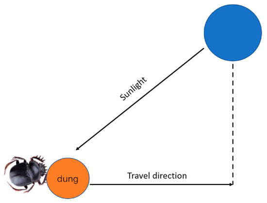
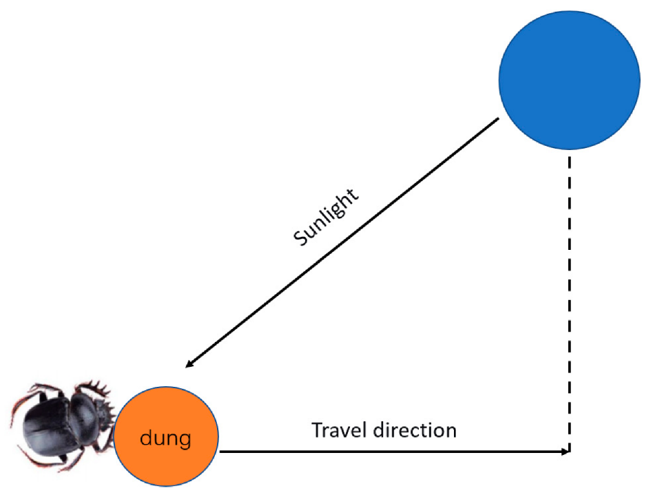
Without any obstructions, the position of the dung beetle in the ball-rolling behavior is influenced by the intensity of sunlight, as shown in Figure 1. The position update formula is shown as Equation (10):

$$\begin{array}{c}\left\{\begin{array}{c}{x}_i\left(t+1\right)=x_i\left(t\right)+\alpha \times k\times x_i\left(t-1\right)+b\times ∆x\\ ∆x=\left|x_i\left(t\right)-X^w\right|\end{array}\right.\end{array}$$

(10)

In the equation, $\alpha =\pm 1$, $k\in (0,0.2)$ represents the deflection coefficient, $b\in (0,1)$ is the random coefficient, $X^w$ represents the globally worst position, and $∆x$ simulates the change in light intensity. The larger the value of $∆x$, the weaker the light intensity, which prompts the dung beetle to avoid this position.

Figure 1. Ball-rolling behavior.

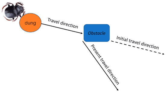
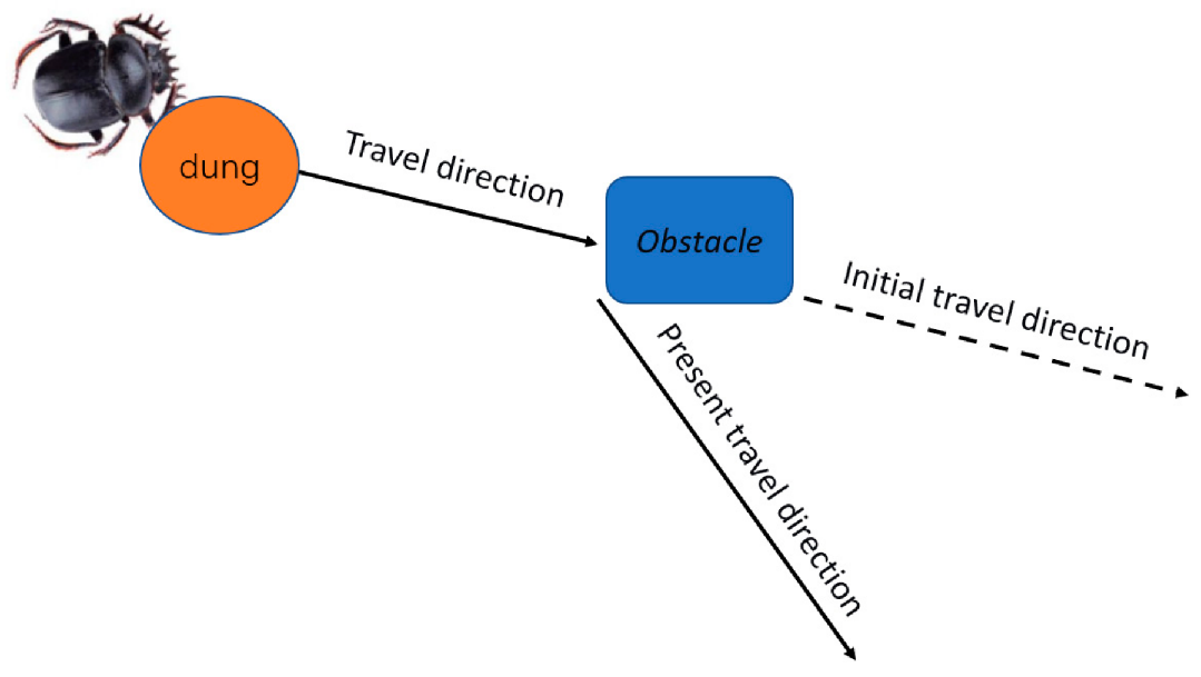
If an obstacle is encountered during the rolling process, the ball-rolling dung beetle will perform a dancing behavior to avoid it, as shown in Figure 2. The formula for updating the position of the dancing behavior is shown as Equation (11):

$$\begin{array}{c}{x}_i\left(t+1\right)=x_i\left(t\right)+tan\left(\theta \right)\left|x_i\left(t\right)-x_i\left(t-1\right)\right|\end{array}$$

(11)

In the equation, $\theta \in (0,\pi )$.

Figure 2. Dancing behavior.

(2)

The behavior of reproduction

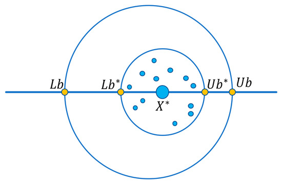
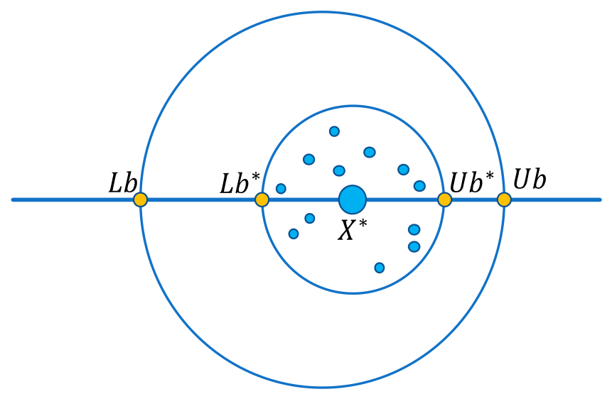
When dung beetles engage in reproductive behavior, they will select an appropriate location for laying eggs, that is, they determine the boundary range. The boundary selection strategy for their egg laying is shown in Figure 3 and Equation (12):

$$\begin{array}{c}\left\{\begin{array}{c}{Lb}^{*}=\mathit{max}\left(X^{*}\times \left(1-R\right),Lb\right)\\ {Ub}^{*}=\mathit{min}\left(X^{*}\times \left(1+R\right),Ub\right)\end{array}\right.\end{array}$$

(12)

In the equation, ${Lb}^{*}$ and ${Ub}^{*}$ denote the lower and upper boundaries of the egg-laying area for dung beetles, while $Lb$ and $Ub$ denote the lower and upper boundaries of the search space. The inertia weight $R=1-{\displaystyle \frac{t}{T}}$, $T$ is the maximum number of iterations, and $X^{*}$ represents the current optimal solution of the population.

Figure 3. Egg-laying area.

From Equation (12), it can be seen that the boundary range of egg-laying is dynamically changing, mainly determined by the inertia weight $R$. This can prevent the algorithm from getting stuck in a local optimal solution. Therefore, the position of the reproduction dung beetle also changes dynamically during the iteration process, and its position update formula is shown as Equation (13):

$$\begin{array}{c}{B}_i\left(t+1\right)=X^{*}+b_1\times \left(B_i\left(t\right)-{Lb}^{*}\right)+b_2\times (B_i\left(t\right)-{Ub}^{*})\end{array}$$

(13)

In the equation, $B_i\left(t\right)$ represents the egg-laying position of the $i$-th reproduction dung beetle in the $t$-th iteration. $b_1$ and $b_2$ are two independent $1\times D$ dimensional random vectors. T is the maximum number of iterations.

(3)

The behavior of foraging

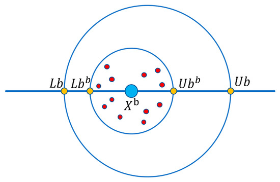
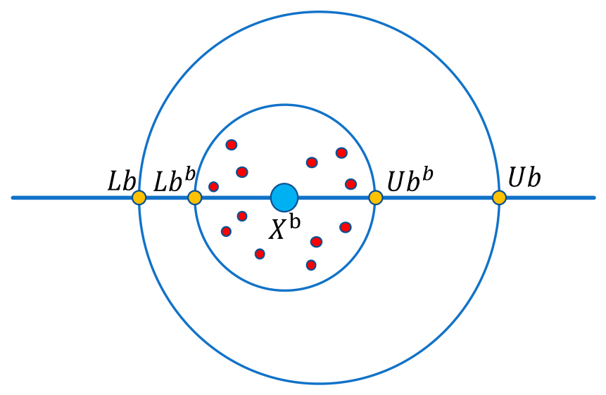
When the small dung beetles hatch successfully, they will come out to engage in foraging behavior. At this point, an optimal foraging area is needed to guide their foraging. The range of this area is shown in Figure 4 and Equation (14):

$$\begin{array}{c}\left\{\begin{array}{c}{Lb}^b=\mathit{max}\left(X^b\times \left(1-R\right),Lb\right)\\ {Ub}^b=\mathit{min}\left(X^b\times \left(1+R\right),Ub\right)\end{array}\right.\end{array}$$

(14)

In the equation, ${Lb}^b$ and ${Ub}^b$ denote the lower and upper boundaries of the foraging area of the small dung beetle, while R is the inertia weight.

Figure 4. Foraging area of the small dung beetle.

After determining the optimal foraging area, based on this area, the method for updating the positions of the small dung beetles (foraging dung beetles) can be defined, which is shown as Equation (15):

$$\begin{array}{c}{x}_i\left(t+1\right)=x_i\left(t\right)+C_1\times \left(x_i\left(t\right)-{Lb}^b\right)+C_2\times (x_i\left(t\right)-{Ub}^b)\end{array}$$

(15)

In the equation, $C_1$ represents a random number that follows a normal distribution, and $C_2$ denote a $1\times D$ dimensional random vector belonging to (0, 1).

(4)

The behavior of stealing

Among the dung beetle populations, there are some dung beetles that steal food from other members of their species. These dung beetles do not randomly choose the location for theft; instead, they tend to act in areas with the richest resources. These areas are usually the high-quality locations that other dung beetles have already discovered and occupied. The update formula for the location of the stealing dung beetles is shown as Equation (16):

$$\begin{array}{c}{x}_i\left(t+1\right)=X^b+S\times g\times (\left|x_i\left(t\right)-X^{*}\right|+\left|x_i\left(t\right)-X^b\right|)\end{array}$$

(16)

where $X^b$ represents the global optimal position, $S$ is a constant, and $g$ is a random vector of size $1\times D$ that follows a normal distribution.

3.2. Improvement of the Dung Beetle Optimizer Algorithm

3.2.1. Initialization Population Strategy Based on Fuch Chaotic Mapping and Reverse Learning

In intelligent optimization algorithms, the quality of the initial population has a significant impact on the global search ability and convergence speed of the algorithm. An excellent initial population and a reasonable population distribution can enable the algorithm to quickly find excellent results, thereby reducing the convergence time. Chaotic mapping has excellent randomness and ergodicity. By using chaotic sequences with nonlinear ergodicity and long-term unpredictability to replace random sequences that follow a standard probability distribution, the distribution of generated individuals becomes more uniform, which can improve the quality of the initial population and help enhance the global optimization ability of the algorithm, thereby improving the performance of the algorithm.

Compared with traditional chaotic mappings such as Logistic and Tent, the Fuch chaotic mapping has the advantages of being insensitive to initial values, having uniform distribution and fast convergence [19]. Therefore, the Fuch chaotic mapping is selected to initialize the dung beetle population. Fu Wenyuan et al. [20] conducted comparative experiments on three chaotic mapping methods—Fuch, Logistic, and Tent—using four classical benchmark functions. The experimental results show that, compared with the other two methods, the Fuch chaotic map significantly reduces the number of function evaluations, improves the efficiency of searching for the global optimum, and validates its high efficiency and practicality in solving optimization problems. Therefore, the Fuch chaotic mapping is selected to initialize the dung beetle population. Its expression is shown as Equation (17).

$$\begin{array}{c}{Fuch}_{i+1}=\mathit{cos}\left({\displaystyle \frac{1}{{Fuch}_i^2}}\right)\end{array}$$

(17)

where ${Fuch}_i$ represents the chaotic variable of the $i$th population of the $Fuch$ mapping, ${Fuch}_i\ne 0$, $i=1,2,\dots ,\mathrm{N}$ and N represents the number of populations.

The reverse learning strategy was proposed by Tizhoosh in 2005. By generating opposite individuals within the current individual region and selecting the individuals with higher fitness for subsequent iterations, it can effectively improve the quality and diversity of the population and enhance the search ability of the algorithm [21]. The population expression obtained through reverse learning is shown as Equation (18).

$$\begin{array}{c}{OBFX}_i={FuchX}_{min}+{FuchX}_{max}-Fuch{X}_i\end{array}$$

(18)

where ${FuchX}_i$ is a population generated through the Fuch chaotic mapping, while ${OBFX}_i$ is a new population generated through reverse learning. Combine the population ${FuchX}_i$ and the reverse population $OBFX\left(n\right)$ according to their fitness levels and select the top $n$ individuals to generate the final initial population.

3.2.2. Improved Ball-Rolling Behavior Integrated with the Vertical Stoop Search Strategy of the Aquila Optimizer

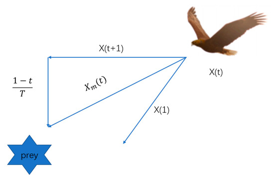
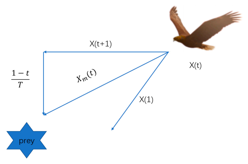
The Aquila optimizer algorithm is a new type of meta-heuristic algorithm, which is inspired by the Aquila’s behaviors in nature during the process of catching the prey. The optimization procedures of the proposed AO algorithm are represented in four methods: selecting the search space by high soar with the vertical stoop, exploring within a diverge search space by contour flight with short glide attack, exploiting within a converge search space by low flight with slow descent attack, and swooping by walk and grab prey [22], as shown in Figure 5.

Figure 5. High soar with vertical stoop.

Based on the ball-rolling behavior of dung beetle, the strategy of Aquila high soar with the vertical stoop is incorporated to expand the range of possible optimal positions. The expression of the improved ball-rolling behaviors is shown as Equations (19) and (20):

$$\begin{array}{c}{x}_i\left(t+1\right)=x_{best}\left(t\right)·\left(1-{\displaystyle \frac{t}{T}}\right)+\left[x_m\left(t\right)-x_{best}\left(t\right)\right]\ast rand\end{array}$$

(19)

$$\begin{array}{c}{x}_m\left(t\right)={\displaystyle \frac{1}{N}}{\displaystyle \sum _{i-1}^N}x\left(t\right),\forall j=1,2,\dots ,dim\end{array}$$

(20)

$x_i\left(t+1\right)$ is the solution of the $\left(t+1\right)$th generation generated by the strategy of Aquila high soar with the vertical stoop, $x_{best}\left(t\right)$ is the optimal solution of the population in the $t$-th iteration, representing the optimal position of the ball-rolling dung beetle population; $x_m\left(t\right)$ is the average value of the current solutions of the population in the $t$-th iteration.

3.3. The Process of the IDBO Algorithm

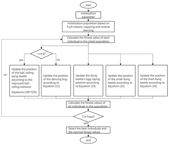
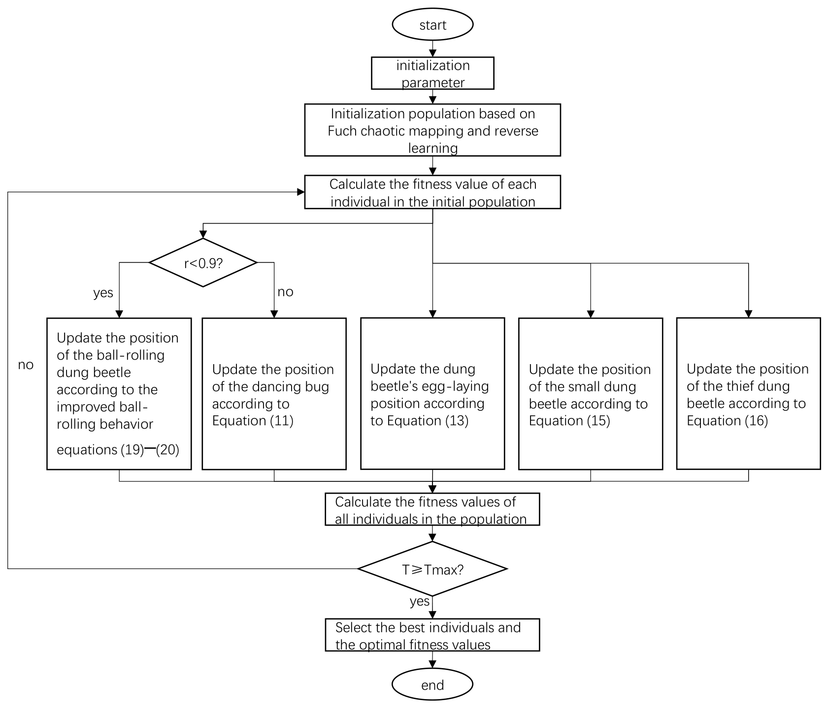
Based on the original DBO algorithm and the improvement strategies in the previous section, the flowchart of the IDBO algorithm is shown in Figure 6.

Figure 6. Flowchart of the algorithm.

Algorithm process steps:

(1)

Set the number of individuals in different behavioral populations in a certain ratio and randomly initialize the population according to the hybrid strategy of Fuch chaotic mapping and reverse learning.

(2)

Calculate the fitness value of each individual in the initial population based on the total evaluation function.

(3)

Select the individuals with the highest and lowest fitness values from the current population and use them for the subsequent update of positions.

(4)

Update the population positions based on the ball-rolling behavior Equations (19) and (20) and the dancing behavior Equation (11).

(5)

Update the egg-laying location based on the egg-laying area Equation (12) and the dung beetle reproductive behavior Equation (13).

(6)

Update the position of the small dung beetle based on the foraging area Equation (14) and the foraging behavior Equation (15).

(7)

Update the population positions based on the theft behavior Equation (16).

(8)

Update the population positions, select the best individual of the current iteration, update the current optimal fitness value, and complete this iteration.

(9)

Determine whether the maximum number of iterations has been reached. If not, repeat steps (3) to (8). If so, proceed to step (10).

(10)

Select the individual with the lowest fitness value from the population, which is the optimal individual obtained by the algorithm.

4. Results

All algorithms were implemented and evaluated using MATLAB R2024a. All tests were performed on a computer with the following specifications: CPU: i7-12700H, GPU: RTX 3060, RAM: 16 G.

4.1. Algorithm Performance and Analysis

4.1.1. Test Functions

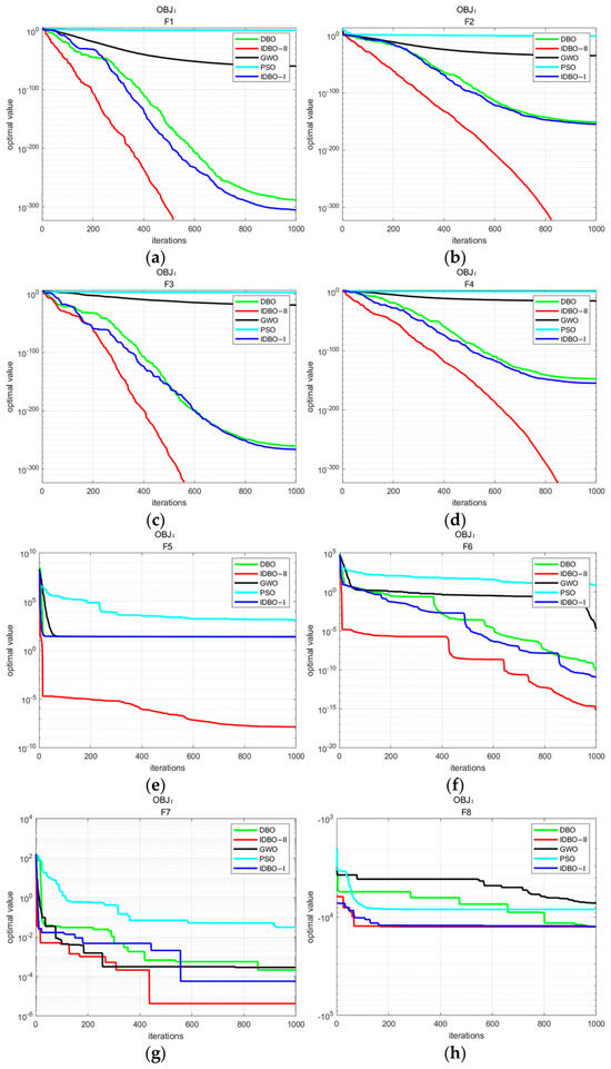
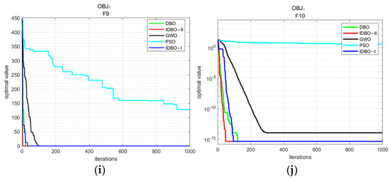
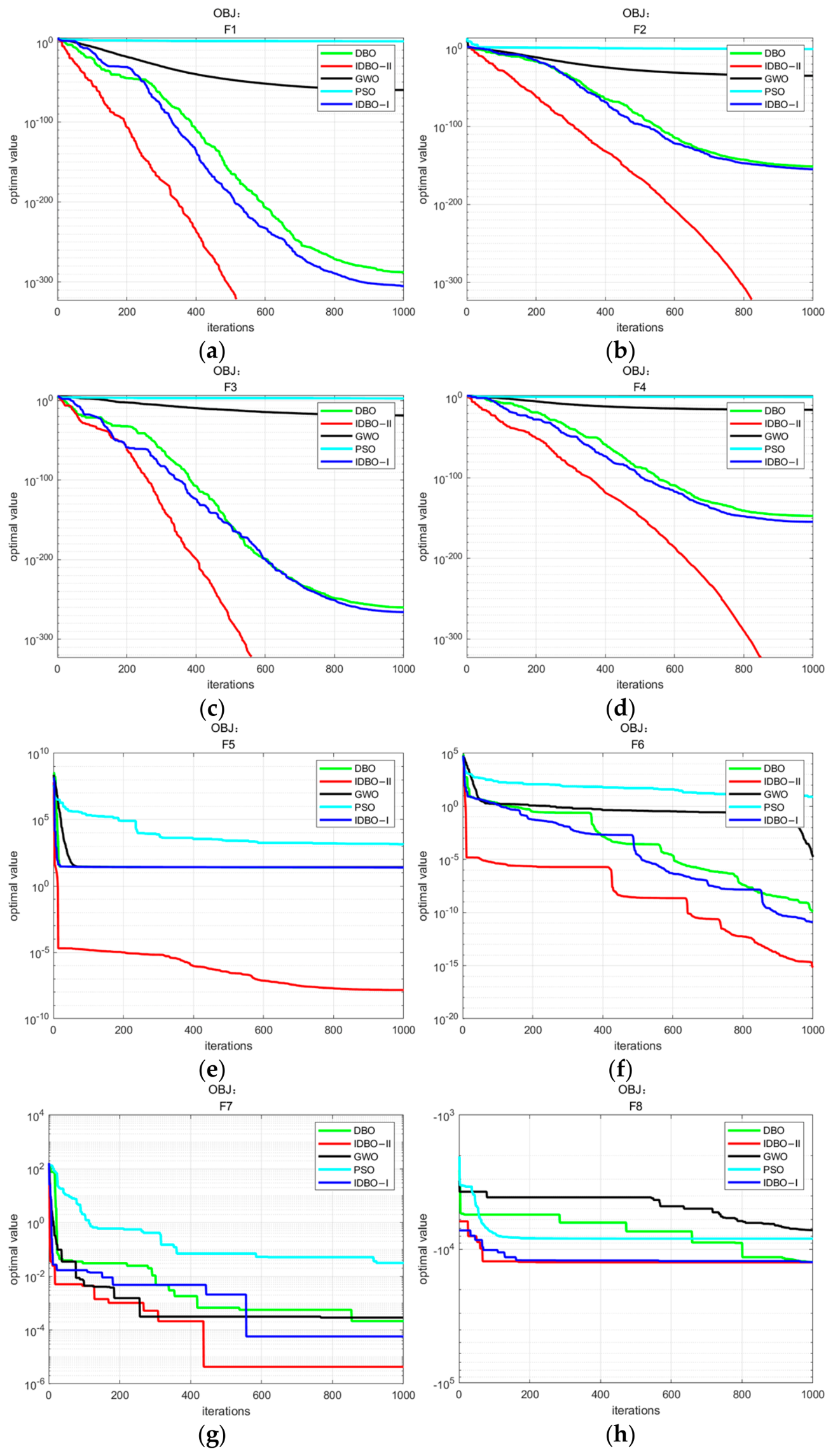
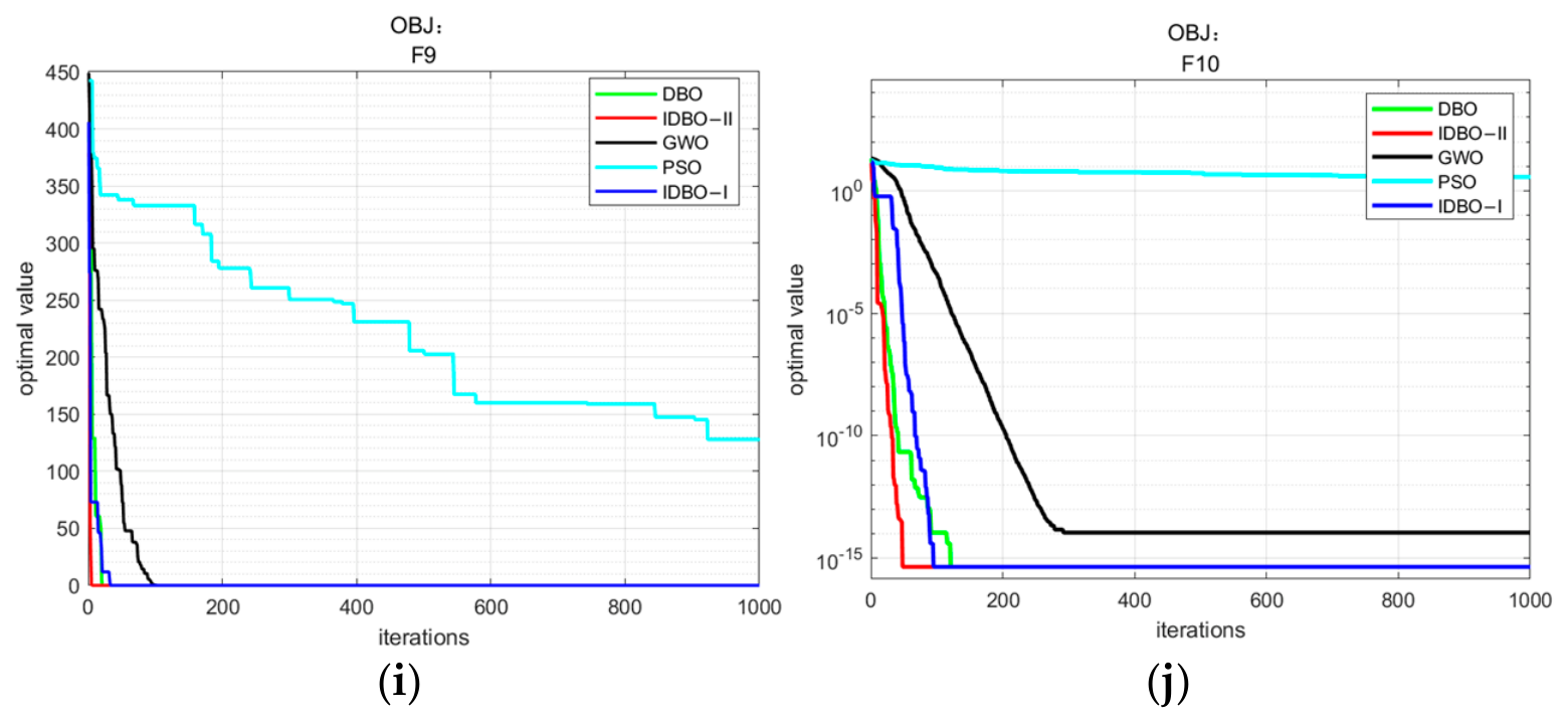
The introduction of the hybrid strategy combining Fuch chaotic mapping and opposition-based learning in the population initialization stage, together with the integration of the vertical stoop search strategy from the Aquila optimizer algorithm in the ball-rolling behavior stage, makes the IDBO algorithm faster in convergence and larger in search range compared with the DBO algorithm, enabling it to find better solutions. To verify the performance of the algorithm, 10 test functions [23] were applied to conduct a comparative test and analysis of the PSO algorithm, which initial particle velocity was set to ±20 [24], the GWO algorithm [25], the original DBO algorithm and the IDBO algorithm. The test functions are shown in Table 1. Among them, F1 to F5 are unimodal test functions, while F6 to F10 are multimodal test functions. The unimodal test functions are mainly used to test the convergence accuracy and convergence speed of the algorithms, while the multimodal test functions primarily assess their ability to escape local optima and their global search capability. In land leveling path planning, the complex field environment and undulating terrain make the algorithms susceptible to falling into local optima. Therefore, the algorithm needs to ensure the convergence accuracy while also having the ability to emerge from local optima and find a better path. Based on relevant literature and the testing process of all algorithms, the population size was set to 30 [26], the number of iterations was 1000, and the test was conducted 20 times. The test data are shown in Table 2, and the convergence curves are presented in Figure 7a–j. To analyze the optimization effects of different improvement strategies in the IDBO algorithm, the algorithm was divided into two optimization stages for performance analysis during the testing process: the IDBO-I algorithm, which only incorporates the population initialization strategy, and the IDBO-II algorithm, which incorporates both the population initialization strategy and the improved ball-rolling behavior strategy.

Table 1. List of test functions.

Test Function	Dimension	Limits	Optimal Value
$F_1\left(x\right)={\sum }_{i=1}^n{x}^2$	30	[−100, 100]	0
$F_2\left(x\right)={\sum }_{i=1}^n\left|x_i\right|+{\prod }_{i=1}^n\left|x_i\right|$	30	[−10, 10]	0
$F_3\left(x\right)={\sum }_{i=1}^n{\left({\sum }_{j=1}^i{x}_j\right)}^2$	30	[−100, 100]	0
$F_4\left(x\right)={max}_i\left\{\left|x_i\right|,1\le i\le n\right\}$	30	[−100, 100]	0
$F_5\left(x\right)={\sum }_{i=1}^{n-1}[100{\left(x_{i+1}-x_i^2\right)}^2+{(x_i-1)}^2]$	30	[−30, 30]	0
$F_6\left(x\right)={\sum }_{i=1}^n{\left(⌊x_i+0.5⌋\right)}^2$	30	[−100, 100]	0
$F_7\left(x\right)={\sum }_{i=1}^{n}i{x}_i^4+random\left[\mathrm{0,1}\right)$	30	[−1.28, 1.28]	0
$F_8\left(x\right)={\sum }_{i=1}^n-x_i\mathrm{s}\mathrm{i}\mathrm{n}\left(\sqrt{\left|x_i\right|}\right)$	30	[−500, 500]	−12,569.5
$F_9\left(x\right)={\sum }_{i=1}^n[x_i^2-10\cos \left(2\pi x_i\right)+10]$	30	[−5.12, 5.12]	0
$F_{10}\left(x\right)=-20\exp \left(-0.2\sqrt{{\displaystyle \frac{1}{n}}{\sum }_{i=1}^n{x}_i^2}\right)-\exp \left({\displaystyle \frac{1}{n}}{\sum }_{i=1}^{n}cos2\pi x_i\right)+20+e$	30	[−32, 32]	0

Table 2. Statistical data of tests.

Test Function	Statistical Data	PSO	GWO	DBO	IDBO-I	IDBO-II
F1	Optimal value	8.9568	1.06 × 10−60	1.61 × 10−288	6.91 × 10−306	0
	average value	15.6811	5.34 × 10−59	5.68 × 10−234	9.65 × 10−249	0
	Standard deviation	4.8638	8.26 × 10−59	2.48 × 10−233	4.21 × 10−248	0
F2	Optimal value	0.2397	1.22 × 10−35	7.68 × 10−152	1.69 × 10−155	0
	average value	14.2248	1.77 × 10−34	1.42 × 10−113	1.42 × 10−126	0
	Standard deviation	15.3004	3.42 × 10−34	6.17 × 10−113	4.31 × 10−126	0
F3	Optimal value	377.7965	1.69 × 10−19	1.20 × 10−260	1.41 × 10−266	0
	average value	571.3986	3.13 × 10−14	3.78 × 10−168	5.30 × 10−189	0
	Standard deviation	135.7675	1.19 × 10−13	1.65 × 10−167	2.31 × 10−188	0
F4	Optimal value	2.7975	3.45 × 10−16	7.46 × 10−148	3.08 × 10−155	0
	average value	7.2381	2.04 × 10−14	7.84 × 10−109	6.98 × 10−123	0
	Standard deviation	2.8009	4.51 × 10−14	2.42 × 10−108	2.51 × 10−122	0
F5	Optimal value	1347.1587	26.0436	24.6346	24.651	1.45 × 10−8
	average value	7657.6593	26.9353	24.9641	24.9557	1.81 × 10−5
	Standard deviation	5118.6967	0.7645	0.1668	0.1779	2.43 × 10−5
F6	Optimal value	7.9124	1.67 × 10−5	1.25 × 10−10	1.28 × 10−11	6.68 × 10−16
	average value	14.1968	0.5340	3.56 × 10−8	1.54 × 10−8	6.10 × 10−12
	Standard deviation	4.0974	0.3196	9.15 × 10−8	5.04 × 10−8	1.11 × 10−11
F7	Optimal value	3.15 × 10−2	2.91 × 10−4	2.16 × 10−4	5.77 × 10−5	4.26 × 10−6
	average value	0.7467	8.84 × 10−4	6.32 × 10−4	5.39 × 10−4	3.02 × 10−5
	Standard deviation	2.0347	4.96 × 10−4	2.85 × 10−4	5.08 × 10−4	2.57 × 10−5
F8	Optimal value	−8360.6	−7224	−12,497	−12,534.7	−12,567.5
	average value	−6683.69	−5888.46	−10,065.1	−11,529.2	−12,361.1
	Standard deviation	886.7645	788.0237	1866.098	1789.103	188.242
F9	Optimal value	127.8859	0	0	0	0
	average value	181.9912	1.42 × 10−14	0	0	0
	Standard deviation	26.7792	2.46 × 10−14	0	0	0
F10	Optimal value	3.6426	1.11 × 10−14	4.44 × 10−16	4.44 × 10−16	4.44 × 10−16
	average value	4.6889	1.55 × 10−14	4.44 × 10−16	4.44 × 10−16	4.44 × 10−16
	Standard deviation	0.7187	2.72 × 10−15	9.86 × 10−32	9.86 × 10−32	9.86 × 10−32

Figure 7. Convergence curve (a) F1; (b) F2; (c) F3; (d) F4; (e) F5; (f) F6; (g) F7; (h) F8; (i) F9; (j) F10.

4.1.2. Performance Testing and Analysis

From the analysis of the results in Table 2, it can be seen that for the unimodal test functions F1–F5, in terms of the best value, the IDBO-II algorithm is able to find the optimal value on functions F1~F4, while none of the other algorithms can find the optimal value. The data indicate that the IDBO-I algorithm, which only incorporates the initialization strategy based on Fuch chaotic mapping and opposition-based learning, outperforms the other three algorithms (excluding IDBO-II) in terms of the best value on all unimodal functions except F5. The IDBO-II algorithm enhances the optimization capability on the basis of IDBO-I. In terms of the mean value over multiple runs, the IDBO-I algorithm is superior to the other three algorithms except IDBO-II. For the IDBO-II algorithm, the mean values on F1~F4 are all equal to their optimal values, and the mean value on F5 is 1.81 × 10⁻⁵, which is closer to the theoretical optimum than those of the other algorithms. This indicates that the IDBO-I algorithm already has a clear advantage over the DBO, PSO, and GWO algorithms on unimodal functions, while the IDBO-II algorithm outperforms IDBO-I in terms of performance. In terms of the standard deviation over multiple runs, the IDBO-I algorithm is better than the other three algorithms (excluding IDBO-II) on all unimodal functions except F5. The standard deviation of the IDBO-II algorithm is 0 on F1~F4, indicating that the algorithm can find the optimal value in every run for these functions. On F5, the standard deviation of the IDBO-II algorithm is 2.43 × 10⁻⁵, which is still better than those of the other algorithms. This clearly confirms the effect of the introduced improvement strategies on enhancing the performance of the DBO algorithm and demonstrates that the IDBO-II algorithm has better stability and robustness in unimodal function tests.

The multimodal test functions F6~F10 place greater emphasis on examining the algorithms’ global search capability and their ability to emerge from local optima. In particular, function F10 has 10³⁰ local optima. In terms of the best value, the IDBO-I algorithm still ranks second only to the IDBO-II algorithm on F6~F8. The best values found by the IDBO-II algorithm on F6~F8 are closer to the true optimal values than those found by the other algorithms. On F9 and F10, the best values found by the IDBO-II algorithm are consistent with those of the DBO and IDBO-I algorithms and superior to those of the PSO and GWO algorithms. Specifically, the IDBO-II algorithm finds the optimal value of 0 on F9, and the best value on F10 is 4.44 × 10⁻¹⁶. These results indicate that the IDBO-II algorithm has better optimization capability and higher solution accuracy on multimodal functions than the other four algorithms. In terms of the mean value over multiple runs, the results of the IDBO-II algorithm on F6~F8 are better than those of the other algorithms. On F9 and F10, its results are consistent with those of the DBO and IDBO-I algorithms and are superior to the PSO and GWO algorithms. The mean values are equal to the optimal values. This demonstrates that the IDBO-II algorithm achieves better overall solution quality on multimodal functions compared with the other four algorithms. In terms of the standard deviation over multiple runs, the IDBO-II algorithm performs better than the other four algorithms on F6~F8. The IDBO-I algorithm outperforms the other three algorithms (excluding IDBO-II) on F6 and F8, but its value on F7 is 5.08 × 10⁻⁴, which is slightly worse than the DBO algorithm’s 2.85 × 10⁻⁴. On F9 and F10, the standard deviation results of the IDBO-II algorithm are consistent with those of the DBO and IDBO-I algorithms and superior to those of the PSO and GWO algorithms. This indicates that the IDBO-II algorithm has better stability and robustness in multimodal function tests. From the convergence curves of the algorithms on the test functions shown in Figure 7a–j, it can be observed that the IDBO-II algorithm exhibits faster overall convergence speed and stronger optimization capability. In summary, the IDBO-II algorithm designed in this chapter has achieved improvements in optimization accuracy, overall solution quality, the ability to escape local optima, stability, and robustness compared with the original dung beetle optimizer algorithm.

4.2. Path Planning Experiments and Results

4.2.1. Data Collection

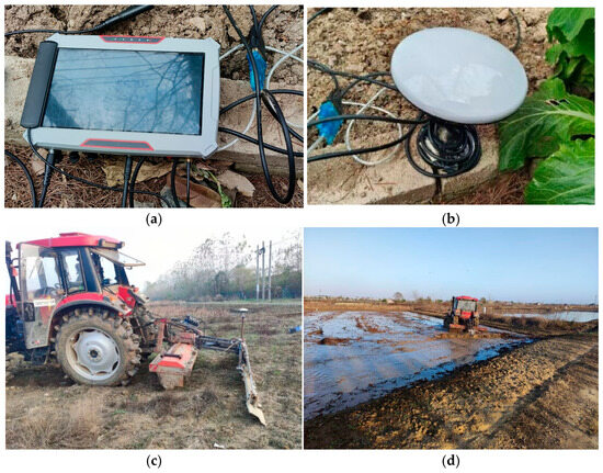
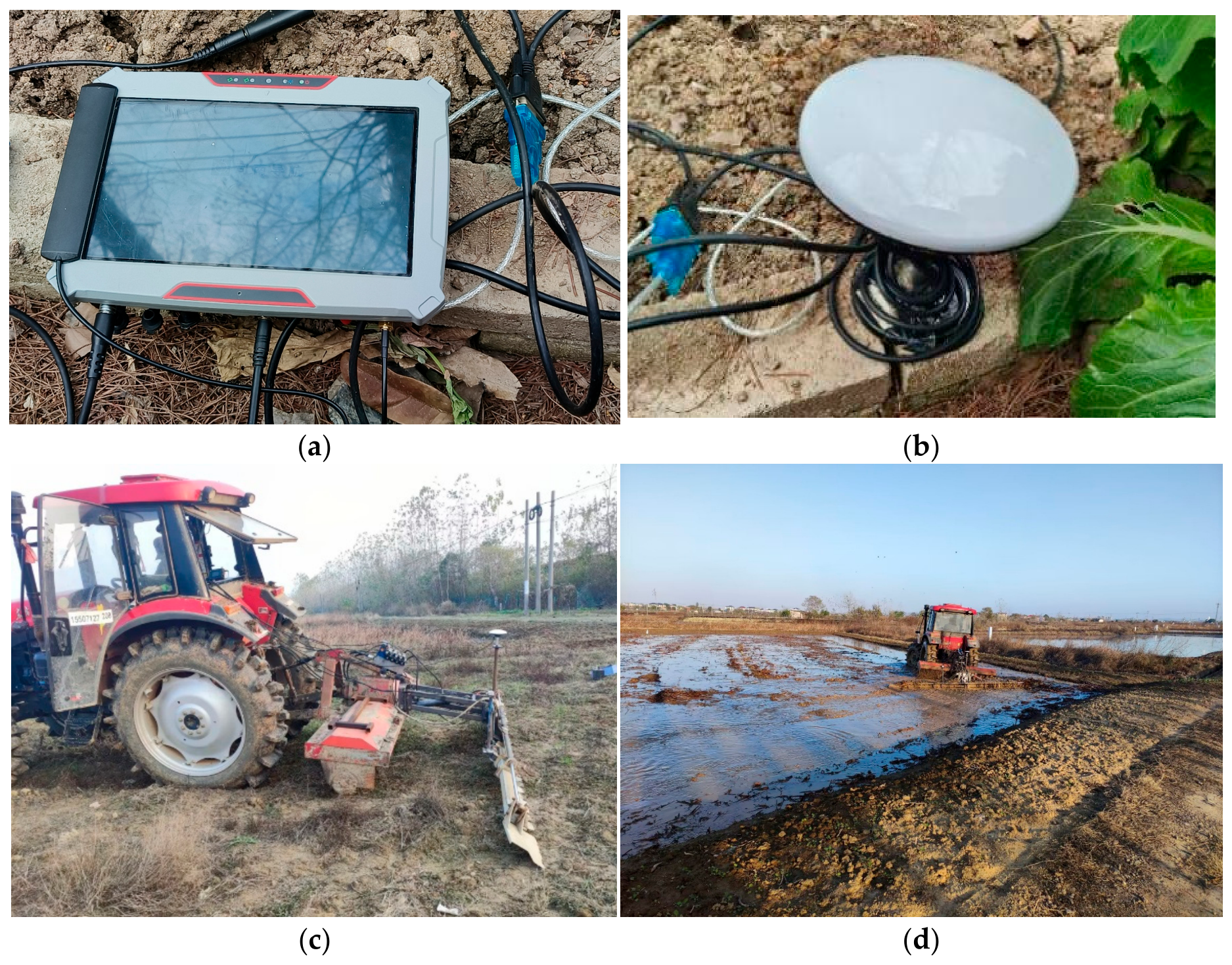
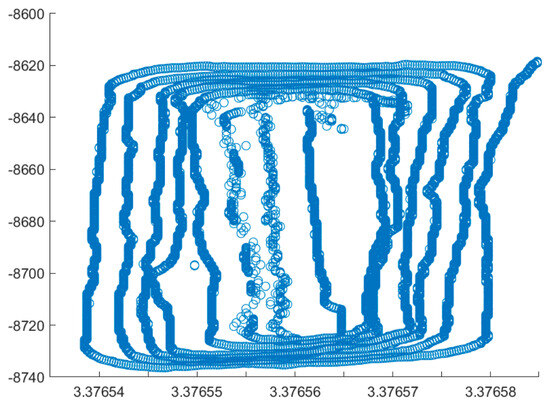
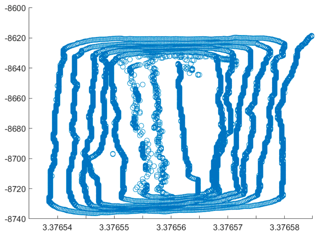
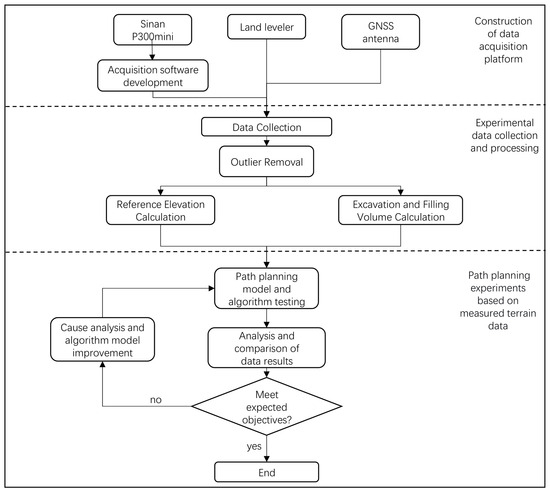
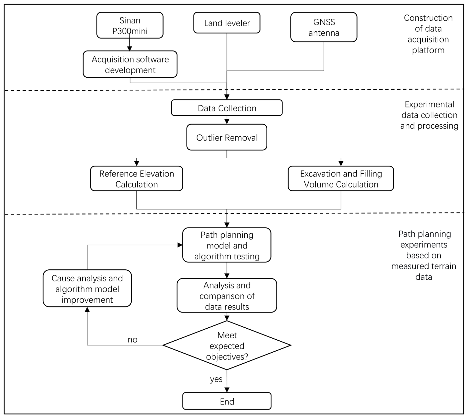
To verify the feasibility of the proposed path planning method, a field of approximately 40 m × 120 m was selected in Putuan Township, Huarong District, Ezhou City. An experimental workflow was designed, covering the entire process from the construction of the data collection platform, data acquisition and processing to the experiments and data analysis. The farmland terrain data collection platform and collection scene are shown in Figure 8. The field data survey trajectory are shown in Figure 9, respectively, and the experimental workflow is shown in Figure 10.

Figure 8. Farmland terrain data collection platform: (a) Mobile acquisition terminal P300mini. (b) GNSS antenna. (c) Paddy field land leveler. (d) Collection scene.

Figure 9. Survey trajectory.

Figure 10. Experimental workflow.

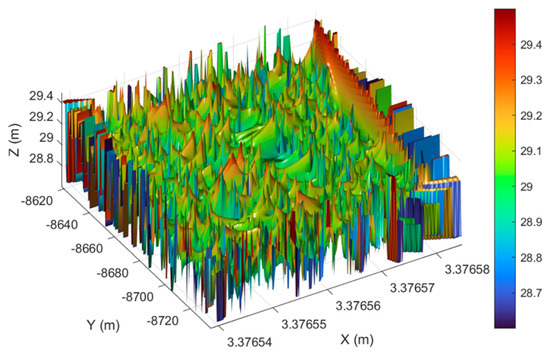
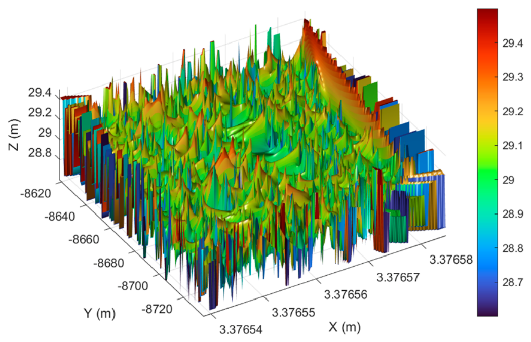
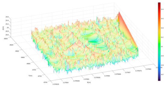
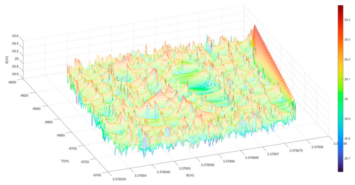
In this paper, a farmland terrain data collection platform was constructed, mainly composed of a Sinan P300mini manufactured by ComNav Technology Ltd., Shanghai, China; a 4G antenna provided by Shenzhen Zhixing Tianbo Technology Co., Ltd., Shenzhen, China; a GNSS antenna produced by Qianxun Spatial Intelligence Inc., Shanghai, China and a paddy field land leveler provided by Ezhou Dinar Technology Co., Ltd., Ezhou, China, as shown in Figure 8a–c. During data collection, the leveling shovel attached to the rear of the land leveler remained in a free-floating state; as the leveling shovel followed the terrain undulations, the acquisition terminal collected the corresponding three-dimensional terrain data. The driver followed a spiral path to collect the three-dimensional terrain data of the target farmland. The original terrain data were then read into MATLAB to generate the original terrain map, as shown in Figure 11.

Figure 11. Original terrain model.

(1)

Coarse filtering is performed to remove boundary outliers. A safe data threshold is set, and data exceeding this threshold are removed.

(2)

Fine filtering is then carried out using the interquartile range (IQR) method to remove outliers within the data, thereby improving terrain smoothness.

The processed terrain is shown in Figure 12.

Figure 12. Processed terrain model.

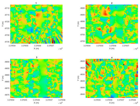
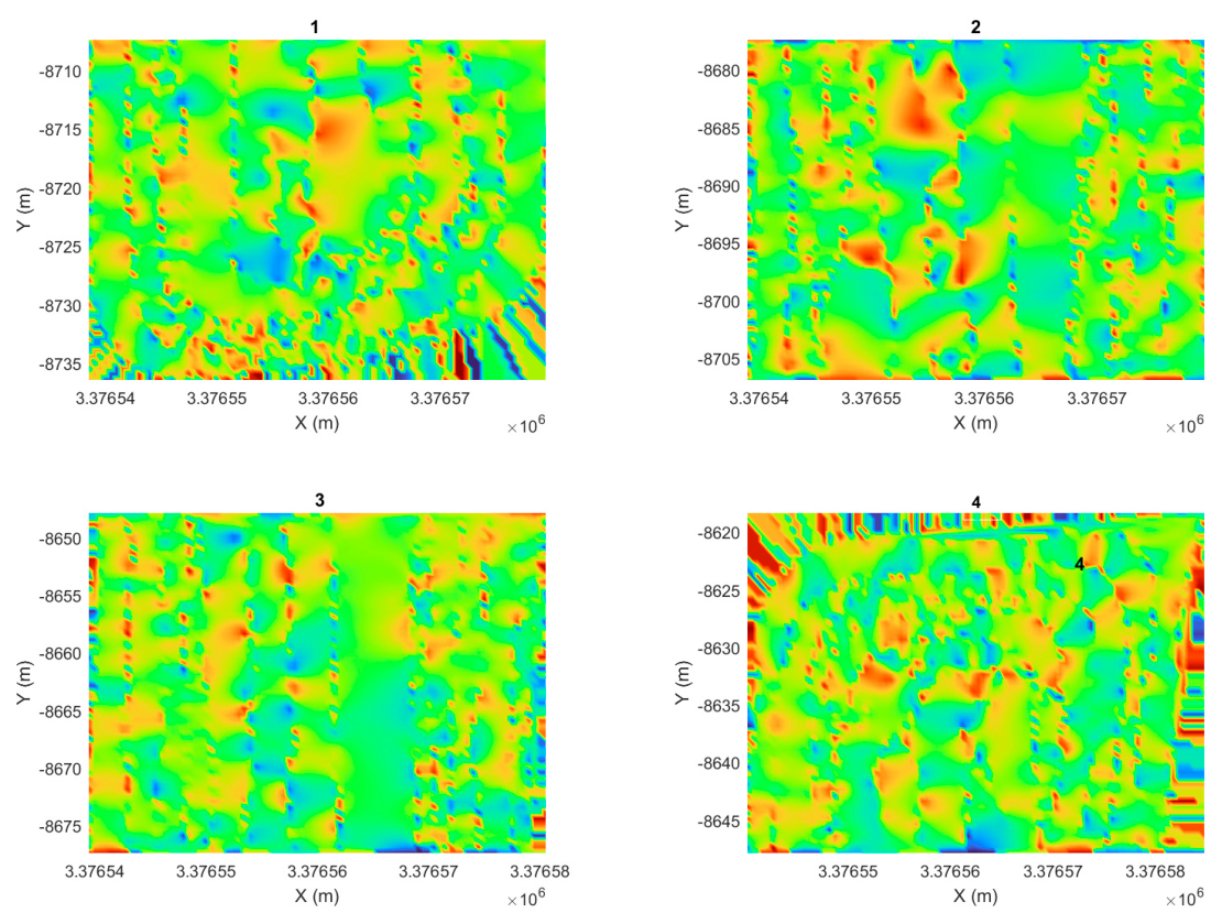
Since this study focuses on local path planning for the land leveler, an excessively large field is not necessary. Therefore, the field was divided into four equal subplots of approximately 40 m × 30 m along the Y-axis as shown in Figure 13. For each subplot, one highest point and one lowest point were randomly selected as the start and end points of the path planning task. Based on relevant literature [26] and the testing process of all algorithms, the population size of all algorithms was set to 30, and the number of iterations was set to 500. For the PSO algorithm, the initial particle velocity was set to ±20 [24]. Each algorithm was run 10 times on each of the four subplots, and the best value and the mean value were recorded.

Figure 13. Divided plots.

4.2.2. Results Analysis

According to the requirements of the land leveling operation on this field, the local operation path planning for the land leveler in this chapter takes the effective operation amount (load variation cost $V_p$) as the primary optimization objective, the leveling quality (under-excavation cost $f_{cut}$ and under-filling cost $f_{fill}$) as the secondary optimization objective, and the energy consumption (path length cost $f_{dist}$) as the tertiary optimization objective. Specifically, a larger $V_p$ indicates a greater effective operation amount of the land leveler; a smaller ${f_{cut}+f}_{fill}$ indicates better leveling quality; and a shorter $f_{dist}$ indicates lower energy consumption. In the total evaluation function Equation (1), the weighting coefficients for the path length cost, under-excavation cost, under-filling cost, and load variation cost are set as ${\omega }_1=1,{\omega }_2={\omega }_3={10}^3,{\omega }_4={10}^6$, respectively. This weighting system can be adjusted according to different land leveling operation requirements. The calculation results of local operation path planning for each subplot are presented below.

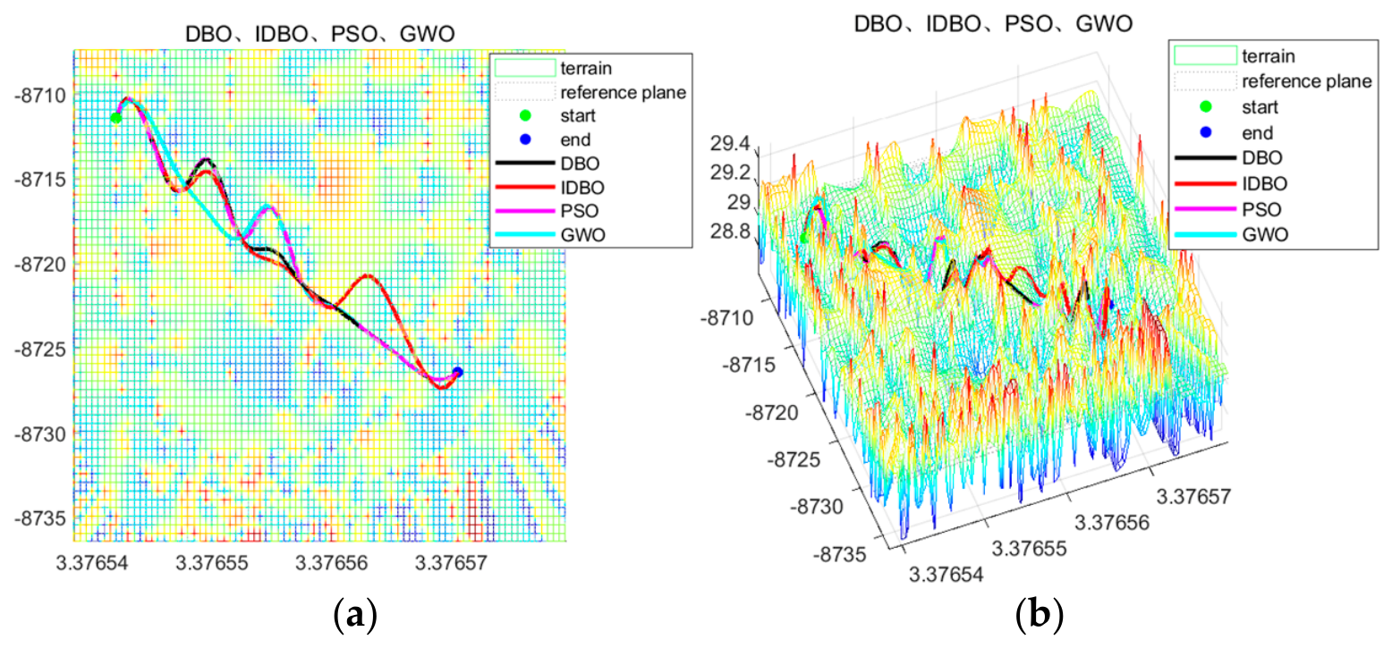
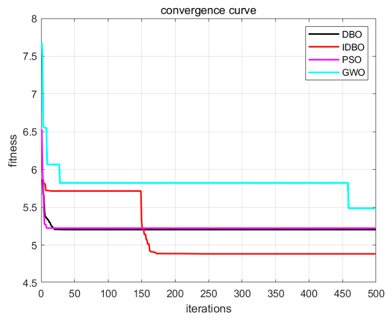
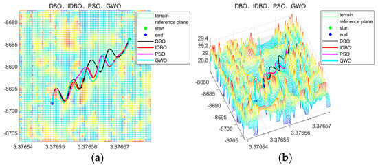
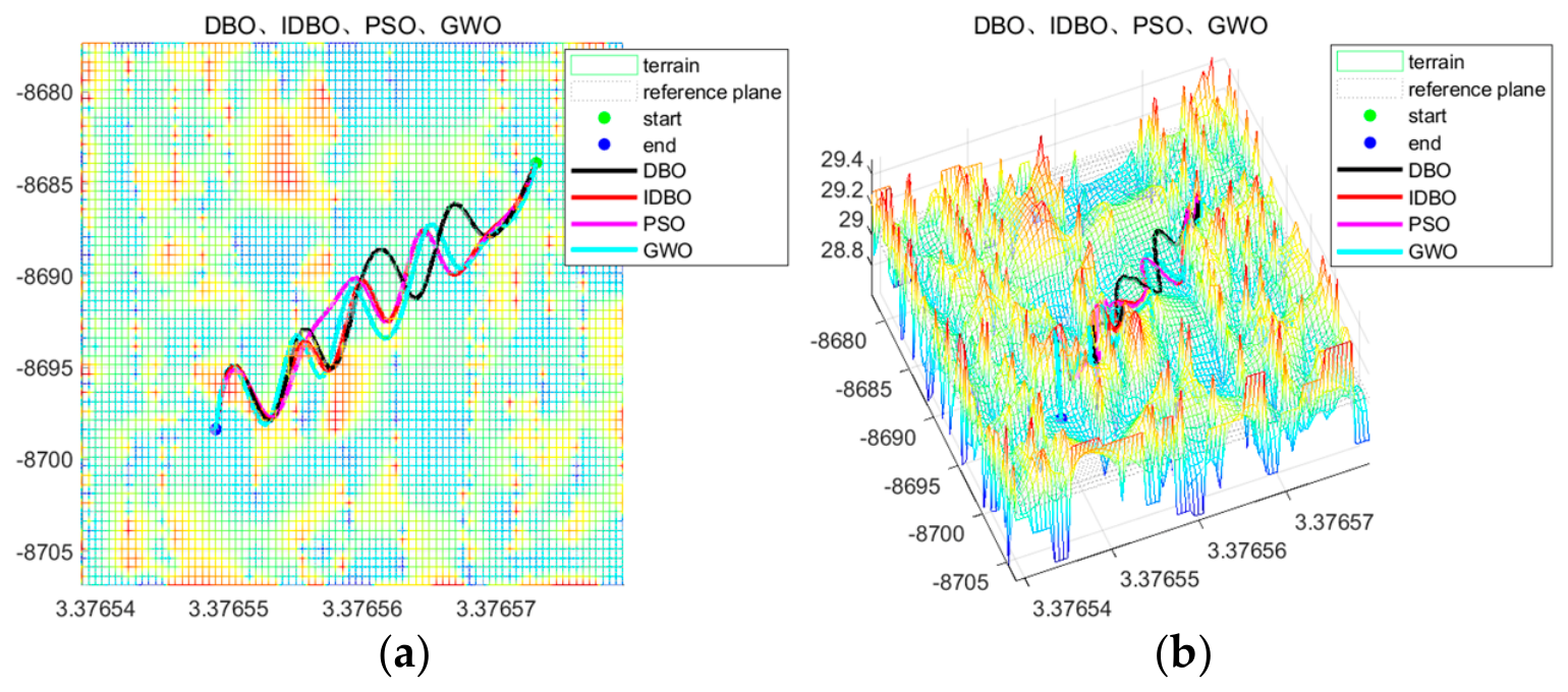
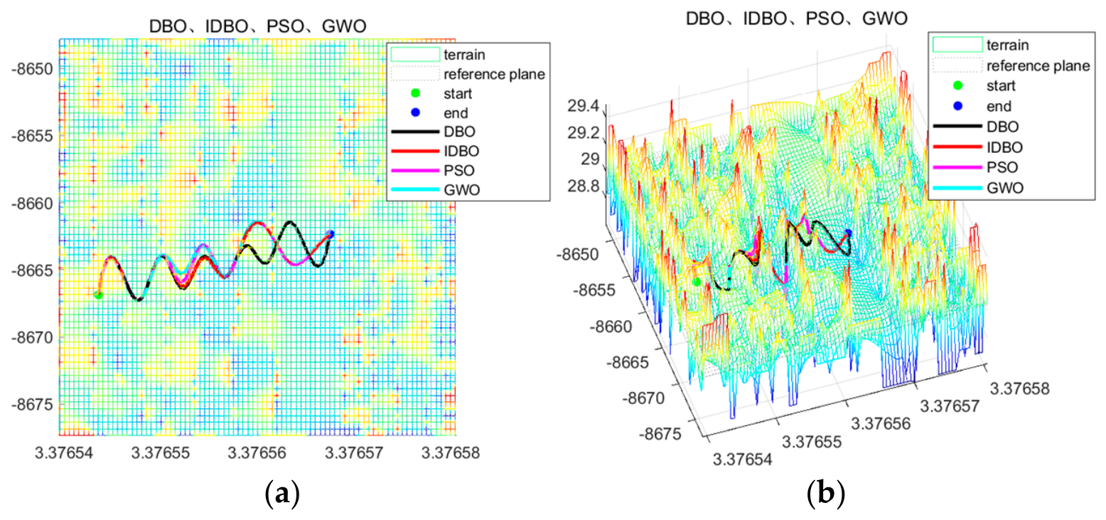
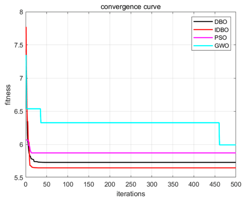
Figure 14a,b present the local operation path planning maps generated by the four algorithms for Plot 1. It can be observed from the figures that all four algorithms are capable of generating effective local operation paths in Plot 1. As shown by the convergence curves in Figure 15, all four algorithms exhibit favorable convergence performance; however, the IDBO algorithm is clearly able to obtain solutions with better fitness.

Figure 14. (a) Plan view of the path for Plot 1; (b) 3D view of the path for Plot 1.

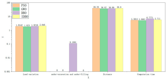
Figure 15. Convergence curves for Plot 1.

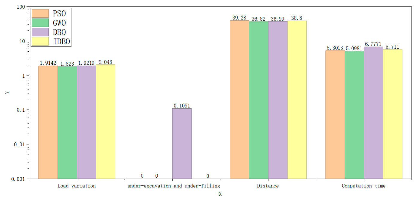
From Table 3 and Figure 16, it can be seen that in the local operation path planning experiment for Plot 1, in terms of the best value, the load variation $V_p$ of the path planned by the IDBO algorithm is 2.0480, which outperforms the other three algorithms, indicating that the land leveler will achieve a larger effective operation amount when traveling along this path and can perform earth excavation and filling more efficiently. The total under-excavation and under-filling volume is 0, which is equal to those of the PSO and GWO algorithms and superior to that of the DBO algorithm. The path length is 38.8, which is superior only to that of the PSO algorithm. This suggests that the load variation is not positively correlated with the total under-excavation and under-filling volume and the path length. During the operation, in order to maintain a high effective operation amount, the land leveler may sacrifice some leveling quality. Meanwhile, within a certain range, it may deviate from the straight trajectory between the start and end points to actively seek areas in need of earth excavation and filling, thereby performing more effective earth excavation and filling operations, which results in a longer path length.

Table 3. Path planning results for Plot 1.

Path Metrics	Result Comparison
	PSO		GWO		DBO		IDBO
	Best	Mean	Best	Mean	Best	Mean	Best	Mean
Load variation $\left(V_p\right)$	1.9142	1.7777	1.8230	1.7453	1.9219	1.8216	2.0480	1.8849
Total under-excavation and under-filling volume $(f_{cut}+f_{fill})$	0	0.0644	0	0.0630	0.1091	0.0109	0	0.0066
Distance/m $\left(f_{dist}\right)$	39.28	36.91	36.82	36.09	36.99	34.71	38.8	35.96
Computation time/s	5.3013	5.1413	5.0981	5.1281	6.7771	5.3536	5.711	5.2497

Figure 16. Comparison histogram for Plot 1.

In terms of the mean value, the load variation $V_p$ of the path planned by the IDBO algorithm is 1.8849 and the total under-excavation and under-filling volume is 0.0066, both of which are superior to those of the other three algorithms, demonstrating that the IDBO algorithm achieves the best overall stability and optimization performance in the path planning process for Plot 1.

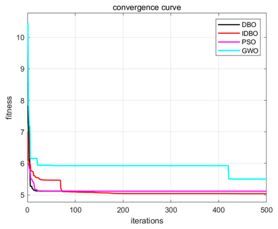
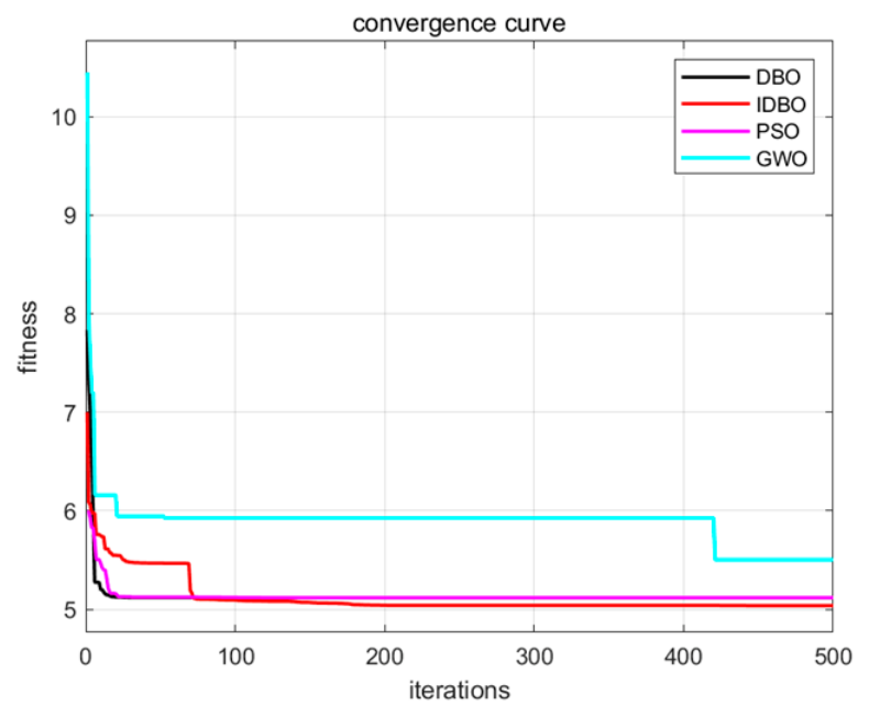
Figure 17a,b present the local operation path planning maps generated by the four algorithms for Plot 2. It can be observed from the figures that all four algorithms are capable of generating effective local operation paths in Plot 2. As shown by the convergence curves in Figure 18, all four algorithms exhibit favorable convergence performance; however, the IDBO algorithm is able to obtain solutions with better fitness.

Figure 17. (a) Plan view of the path for Plot 2; (b) 3D view of the path for Plot 2.

Figure 18. Convergence curves for Plot 2.

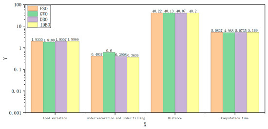
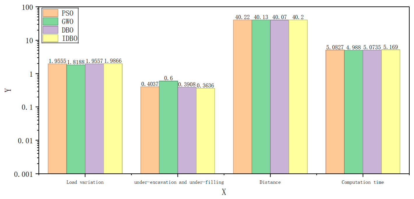
From Table 4 and Figure 19, it can be seen that in the local operation path planning experiment for Plot 2, in terms of the best value, the load variation $V_p$ of the path planned by the IDBO algorithm is 1.9866, which outperforms the other three algorithms, indicating that the land leveler can perform earth excavation and filling more efficiently when traveling along this path. The total under-excavation and under-filling volume is 0.3636, which is superior to those of the other three algorithms. The path length is 40.20, which is superior only to that of the PSO algorithm, but the differences from the GWO and DBO algorithms are very small. This indicates that the optimal path is able to maintain a high effective excavation and filling amount while achieving favorable leveling quality and energy consumption.

Table 4. Path planning results for Plot 2.

Path Metrics	Result Comparison
	PSO		GWO		DBO		IDBO
	Best	Mean	Best	Mean	Best	Mean	Best	Mean
Load variation $\left(V_p\right)$	1.9555	1.7987	1.8188	1.7522	1.9557	1.8234	1.9866	1.9088
Total under-excavation and under-filling volume $\left({f_{cut}+f}_{fill}\right)$	0.4037	0.4020	0.6000	0.4517	0.3908	0.2337	0.3636	0.2492
Distance/m ${(f}_{dist})$	40.22	38.73	40.13	40.55	40.07	37.50	40.20	38.98
Computation time/s	5.0827	5.0929	4.988	5.0892	5.0735	5.1451	5.169	5.1834

Figure 19. Comparison histogram for Plot 2.

In terms of the mean value, the load variation $V_p$ of the path planned by the IDBO algorithm is 1.9088, which outperforms the other three algorithms, demonstrating that the IDBO algorithm achieves the best overall stability and optimization performance in the path planning process for Plot 2.

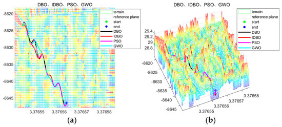
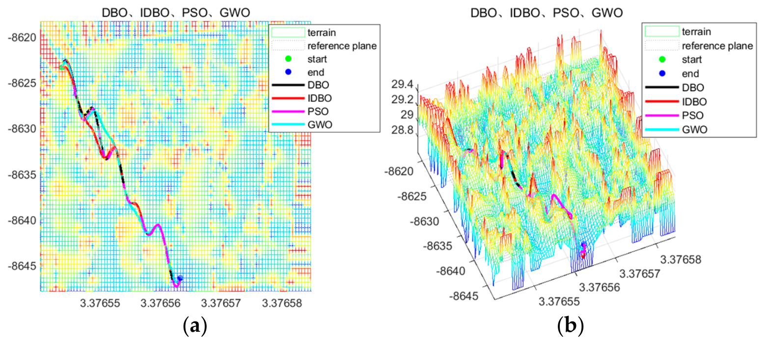
Figure 20a,b present the local operation path planning maps generated by the four algorithms for Plot 3. It can be observed from the figures that all four algorithms are capable of generating effective local operation paths in Plot 3. As shown by the convergence curves in Figure 21, all four algorithms exhibit favorable convergence performance; however, the IDBO algorithm is able to obtain solutions with better fitness.

Figure 20. (a) Plan view of the path for Plot 3; (b) 3D view of the path for Plot 3.

Figure 21. Convergence curves for Plot 3.

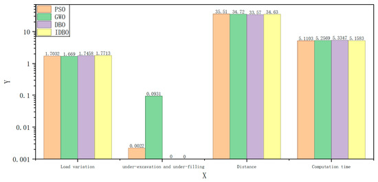
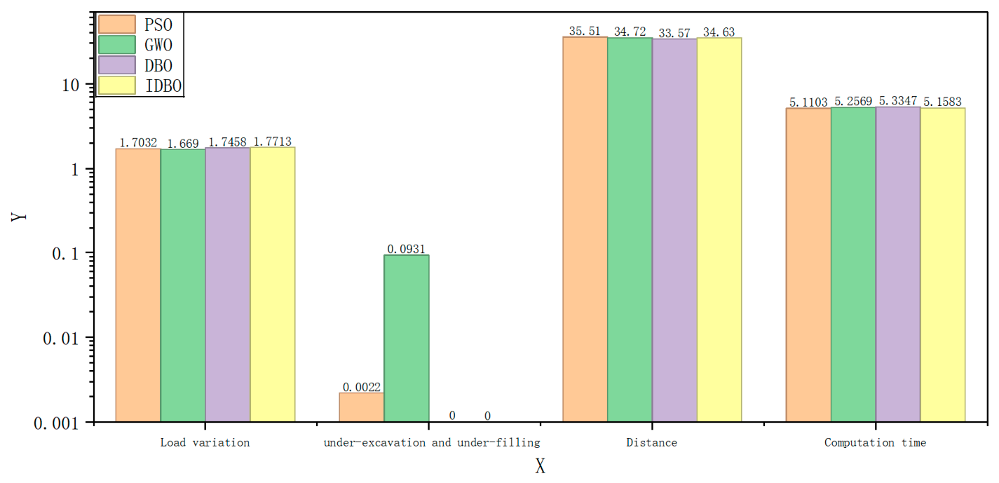
From Table 5 and Figure 22, it can be seen that in the local operation path planning experiment for Plot 3, in terms of the best value, the load variation $V_p$ of the path planned by the IDBO algorithm is 1.7713, which outperforms the other three algorithms, indicating that the land leveler can perform earth excavation and filling more efficiently when traveling along this path. The total under-excavation and under-filling volume is 0, which is equal to that of the DBO algorithm and superior to those of the PSO and GWO algorithms. The path length is 34.63, which is superior to those of the other three algorithms. This indicates that the optimal path is able to maintain a high effective excavation and filling amount while achieving favorable leveling quality and energy consumption.

Table 5. Path planning results for Plot 3.

Path Metrics	Result Comparison
	PSO		GWO		DBO		IDBO
	Best	Mean	Best	Mean	Best	Mean	Best	Mean
Load variation $\left(V_p\right)$	1.7032	1.6284	1.6690	1.5811	1.7458	1.6550	1.7713	1.7241
Total under-excavation and under-filling volume $\left({f_{cut}+f}_{fill}\right)$	0.0022	0.0003	0.0931	0.0381	0	0	0	0
Distance/m ${(f}_{dist})$	35.51	34.08	34.72	34.97	36.82	33.57	34.63	32.47
Computation time/s	5.1103	5.1755	5.2569	5.1605	5.3347	5.3347	5.1583	5.2427

Figure 22. Comparison histogram for Plot 3.

In terms of the mean value, the load variation $V_p$ of the path planned by the IDBO algorithm is 1.7241, which outperforms the other three algorithms, demonstrating that the IDBO algorithm achieves the best overall stability and optimization performance in the path planning process for Plot 3.

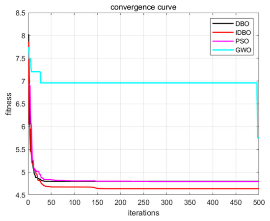
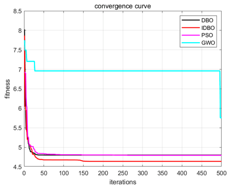
Figure 23a,b present the local operation path planning maps generated by the four algorithms for Plot 4. It can be observed from the figures that all four algorithms are capable of generating effective local operation paths in Plot 4. As shown by the convergence curves in Figure 24, the IDBO algorithm is able to obtain solutions with better fitness.

Figure 23. (a) Plan view of the path for Plot 4; (b) 3D view of the path for Plot 4.

Figure 24. Convergence curves for Plot 4.

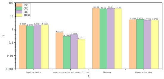
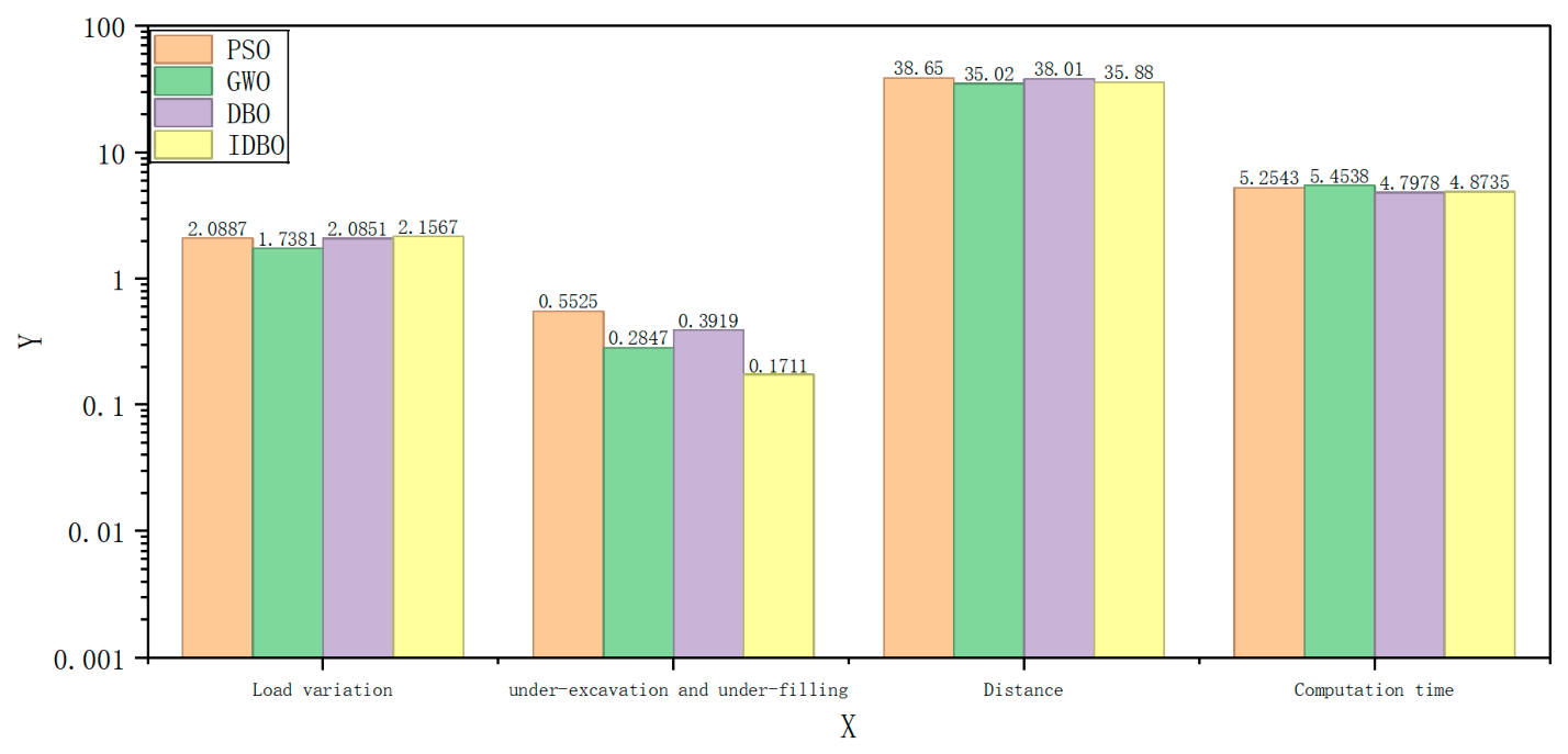
From Table 6 and Figure 25, it can be seen that in the local operation path planning experiment for Plot 4, in terms of the best value, the load variation $V_p$ of the path planned by the IDBO algorithm is 2.1567, which outperforms the other three algorithms, indicating that the land leveler can perform earth excavation and filling more efficiently when traveling along this path. The total under-excavation and under-filling volume is 0.1711, which is superior to those of the other three algorithms. The path length is 35.88, which is superior only to that of the PSO algorithm. The three key indicators were not optimized simultaneously; however, the superiority of the primary optimization objective was guaranteed.

Table 6. Path planning results for Plot 4.

Path Metrics	Result Comparison
	PSO		GWO		DBO		IDBO
	Best	Mean	Best	Mean	Best	Mean	Best	Mean
Load variation $\left(V_p\right)$	2.0887	1.8468	1.7381	1.5983	2.0851	1.9070	2.1567	2.0351
Total under-excavation and under-filling volume $\left({f_{cut}+f}_{fill}\right)$	0.5525	0.4695	0.2847	0.3946	0.3919	0.3388	0.1711	0.3238
Distance/m ${(f}_{dist})$	38.65	36.33	35.02	35.30	38.01	35.84	35.88	36.61
Computation time/s	5.2543	4.8682	5.4538	4.8304	4.7978	4.9709	4.8735	4.9643

Figure 25. Comparison histogram for Plot 4.

In terms of the mean value, the load variation $V_p$ of the path planned by the IDBO algorithm is 2.0351, which outperforms the other three algorithms, demonstrating that the IDBO algorithm achieves the best overall stability and optimization performance in the path planning process for Plot 4.

Based on the experimental results and data analysis for all plots, it can be seen that the proposed algorithm is capable of generating effective operation paths in different field environments. Compared with the other three algorithms, it achieves better fitness values and ensures the superiority of the primary optimization objective. The experimental data and convergence curves demonstrate that the IDBO algorithm designed in this paper exhibits favorable performance and stability in the local operation path planning of the land leveler.

5. Conclusions

(1)

Aiming at the local path planning problem of the land leveler, this paper comprehensively considers factors such as path length, the balance of earth excavation and filling, and the total amount of excavated and filled soil when modeling the land leveling operation, and establishes a weighted objective function for the land leveler operation path.

(2)

Based on the original DBO algorithm, an improved DBO algorithm (IDBO) is designed in this paper to solve the objective function of land leveler operation path planning. In the population initialization stage, a hybrid strategy combining Fuch chaotic mapping and opposition-based learning is introduced to enhance the diversity of the initial population. In the ball-rolling behavior stage, the vertical stoop search strategy from the Aquila optimizer algorithm is incorporated to expand the search range and increase the convergence speed. Ten benchmark functions are used to compare the IDBO algorithm with the PSO algorithm, the GWO algorithm and the original DBO algorithm. The superiority of the IDBO algorithm is verified through the computational results and convergence curves.

(3)

A three-dimensional farmland terrain model was established based on field data collected in situ. Path planning experiments for the land leveler were conducted using the collected farmland data. In terms of the solution to the objective function for the operation path planning of the land leveler, the IDBO algorithm outperforms the DBO algorithm, the PSO algorithm, and the GWO algorithm, The experimental results show that, in terms of the primary optimization objective $V_p$, compared with the other three algorithms (PSO, GWO, DBO), the IDBO algorithm achieved improvements of 7.0%, 12.3%, and 6.6% on Plot 1, 1.6%, 9.2%, and 1.6% on Plot 2, 4.0%, 6.1%, and 1.5% on Plot 3, and 3.3%, 24.1%, and 3.4% on Plot 4. It indicates that the proposed method based on the improved IDBO algorithm is suitable for local operation path planning of land leveler.

(4)

This study has achieved the expected objectives and results in the research on the local operation path planning for the paddy field land leveler. However, it has not been combined with the global operation path planning to form a complete path planning scheme. Moreover, the study is limited to obstacle-free fields. If utility poles or other obstacles exist in the field, the path planning model and algorithm need to be further improved.

(5)

The algorithm proposed in this paper has only been studied using MATLAB software and has not yet been integrated into a systematic application. In future work, the IDBO-based path planning module can be integrated with the automatic driving system of the land leveler, and automatic navigation operations after path planning can be realized through the path tracking algorithm.

References

- Foley, J.A.; Ramankutty, N.; Bennett, E.M.; Brauman, K.A.; Carpenter, S.R.; Cassidy, E.; Gerber, J.; Johnston, M.; Mueller, N.D.; O’Connell, C.; et al. Solutions for a cultivated planet: Addressing our global food production and environmental sustainability challenges. Nature 2011, 478, 337–342. [Google Scholar] [CrossRef] [Scilit]
- Far, S.T.; Rezaei-Moghaddam, K. A socio-psychological model of laser levelling impacts assessment. Genom. Soc. Policy 2020, 16, 2. [Google Scholar] [CrossRef] [Scilit]
- Chen, G.; Hu, L.; Luo, X.; Wang, P.; He, J.; Huang, P.; Zhao, R.; Feng, D.; Tu, T. A review of global precision land-leveling technologies and implements: Current status, challenges and future trends. Comput. Electron. Agric. 2024, 220, 108901. [Google Scholar] [CrossRef] [Scilit]
- Miao, Q.; Gonçalves, J.M.; Li, R.; Gonçalves, D.; Levita, T.; Shi, H. Assessment of Precise Land Levelling on Surface Irrigation Development. Impacts on Maize Water Productivity and Economics. Sustainability 2021, 13, 1191. [Google Scholar] [CrossRef] [Scilit]
- Hashim, S.; Mirani, A.A.; Iqbal, M.N.; Ashraf, W.; Naz, U. Comparative evaluation of water use efficiency through precision land leveling. J. Stat. Comp. Interdis. Res. 2025, 7, 79–102. [Google Scholar] [CrossRef] [Scilit]
- Oztekin, T. Short-term effects of land leveling on irrigation-related some soil properties in a clay loam soil. Sci. World J. 2013, 2013, 187490. [Google Scholar] [CrossRef] [Scilit] [PubMed]
- Ojima, I.; Date, H. Path planning for a land leveler. In Proceedings of the 2019 IEEE/SICE International Symposium on System Integration (SII), Paris, France, 14–16 January 2019; pp. 222–226. [Google Scholar] [CrossRef] [Scilit]
- Jing, Y.; Liu, G.; Luo, C. Path tracking control with slip compensation of a global navigation satellite system based tractor-scraper land levelling system. Biosyst. Eng. 2021, 212, 53–67. [Google Scholar] [CrossRef] [Scilit]
- Jing, Y.; Luo, C.; Liu, G. Multiobjective path optimization for autonomous land levelling operations based on an improved MOEA/D-ACO. Comput. Electron. Agric. 2022, 197, 106995. [Google Scholar] [CrossRef] [Scilit]
- Yang, J. Research on Intelligent Planning Method of Farmland Leveler Operation Path Based on Variable Scale Improved Ant Colony Algorithm. Master’s Thesis, Jiangsu University, Zhenjiang, China, 2024. [Google Scholar] [CrossRef]
- Liu, G.; Li, X.; Kang, X.; Xia, Y.; Niu, D. Automatic navigation path planning method for land leveling based on GNSS. Trans. Chin. Soc. Agric. Mach. 2016, 47, 21–29. [Google Scholar]
- Wang, T. Research on GNSS-Based Farmland Leveling Operation Path Planning. Master’s Thesis, Heilongjiang Bayi Agricultural University, Daqing, China, 2022. [Google Scholar] [CrossRef]
- Xi, X.; Jin, J.; Wang, Y.; Han, L.; Zou, Y.; Zhang, R. Dynamic expansion neighborhood path planning method for satellite navigation grader. Trans. Chin. Soc. Agric. Mach. 2025, 56, 419–426+478. [Google Scholar] [CrossRef]
- Jing, Y.; Jin, Z.; Liu, G. Three dimensional path planning method for navigation of farmland leveling based on improved ant colony algorithm. Trans. Chin. Soc. Agric. Mach. 2020, 51, 333–339. [Google Scholar] [CrossRef]
- Chen, W.; Yang, J.; Zhang, S.; Wei, X.; Liu, C.; Zhou, X.; Sun, L.; Wang, F.; Wang, A. Variable scale operational path planning for land levelling based on the improved ant colony optimization algorithm. Sci. Rep. 2025, 15, 9854. [Google Scholar] [CrossRef] [Scilit]
- Fei, H.; Liu, R.; Dong, L.; Du, Z.; Liu, X.; Luo, T.; Zhou, J. Three-Dimensional Path Planning for Unmanned Aerial Vehicles Based on Hybrid Multi-Strategy Dung Beetle Optimization Algorithm. Agriculture 2025, 15, 1156. [Google Scholar] [CrossRef] [Scilit]
- Liu, L.; Wang, X.; Liu, H.; Li, J.; Wang, P.; Yang, X. A Full-Coverage Path Planning Method for an Orchard Mower Based on the Dung Beetle Optimization Algorithm. Agriculture 2024, 14, 865. [Google Scholar] [CrossRef] [Scilit]
- Xue, J.; Shen, B. Dung beetle optimizer: A new meta-heuristic algorithm for global optimization. J. Supercomput. 2023, 79, 7305–7336. [Google Scholar] [CrossRef] [Scilit]
- Chen, X.; Zhang, S.; Yang, P.; Zhang, Y. Prediction on hot rolled strip width based on improved BOA-ELM. Forg. Stamp. Technol. 2024, 49, 101–106+126. [Google Scholar] [CrossRef]
- Fu, W.; Ling, C. An adaptive iterative chaos optimization method. J. Xi’an Jiaotong Univ. 2013, 47, 33–38. [Google Scholar] [CrossRef]
- Huang, Y.; Li, Y.; Zhang, Z.; Sun, Q. A novel path planning approach for AUV based on improved whale optimization algorithm using segment learning and adaptive operator selection. Ocean. Eng. 2023, 280, 114591. [Google Scholar] [CrossRef] [Scilit]
- Abualigah, L.; Yousri, D.; Abd Elaziz, M.; Ewees, A.A.; Al-qaness, M.A.A.; Gandomi, A.H. Aquila Optimizer: A novel meta-heuristic optimization algorithm. Comput. Ind. Eng. 2021, 157, 107250. [Google Scholar] [CrossRef] [Scilit]
- Yao, X.; Liu, Y. Evolutionary programming made faster. IEEE Trans. Evol. Comput. 1999, 3, 82–102. [Google Scholar] [CrossRef] [Scilit]
- Poli, R.; Kennedy, J.; Blackwell, T. Particle swarm optimization. Swarm Intell. 2007, 1, 33–57. [Google Scholar] [CrossRef] [Scilit]
- Mirjalili, S.; Saremi, S.; Mirjalili, S.M.; Coelho, L.S. Multi-objective grey wolf optimizer: A novel algorithm for multi-criterion optimization. Expert Syst. Appl. 2015, 47, 106–119. [Google Scholar] [CrossRef] [Scilit]
- Jiang, A.; Liu, W. Unmanned aerial vehicle three-dimensional path planning based on improved dung beetle optimization algorithm. Electron. Meas. Technol. 2024, 47, 128–135. [Google Scholar] [CrossRef]
Disclaimer/Publisher’s Note: The statements, opinions and data contained in all publications are solely those of the individual author(s) and contributor(s) and not of MDPI and/or the editor(s). MDPI and/or the editor(s) disclaim responsibility for any injury to people or property resulting from any ideas, methods, instructions or products referred to in the content. |
© 2026 by the authors. Licensee MDPI, Basel, Switzerland. This article is an open access article distributed under the terms and conditions of the Creative Commons Attribution (CC BY) license.