Online Recognition of Partially Developed X-Bar Chart Patterns with Optimized Statistical Feature Set and Recognizer

Abstract

This study addresses the challenge of early-stage recognition of control chart patterns in statistical process control, which is critical for timely detection of process abnormalities in real-time manufacturing environments. Unlike most existing approaches that focus on fully developed patterns, this work targets partially developed patterns within a fixed observation window to enable proactive intervention. A multi-layer perceptron (MLP) classifier was developed using statistical features, and a structured design of experiments (DOE) approach was employed to optimize both the feature set and network parameters. Simulated X-bar chart data representing six pattern types were used, and candidate features were systematically evaluated using fractional factorial design. The results identified an effective feature subset consisting of autocorrelation, mean, mean square value, standard deviation, slope, and cumulative sum. The optimized MLP achieved an offline accuracy of approximately 86%, while online implementation yielded an overall accuracy of 70.6% with acceptable error rates and average run length performance (ARL₀ = 207.3, ARL_I = 10.9). The findings demonstrate that, despite greater difficulty in online recognition, the proposed approach provides a practical and interpretable solution for early detection in quality control systems.

1. Introduction

Unstable processes normally produce time series patterns when visualized on a Shewhart X-bar chart [1]. The knowledge of pattern types is critical for diagnosis and narrowing down possible root causes for unstable processes [2,3]. Generally, the root causes for unnatural patterns could be attributed to specific assignable causes. For example, a sudden shift in the process level may result from a change in machine settings, an inexperienced operator, the introduction of different raw materials, or a minor machine malfunction. A steady upward or downward trend could be caused by tool or die wear, gradual equipment deterioration, slow changes in temperature or humidity, or the accumulation of chips in the work-holding device [4]. Recurring cycles may reflect seasonal variations in incoming materials, repeated fluctuations in temperature or humidity, periodic chemical or mechanical influences, psychological factors, or routine rotation of operators [5].

Over the past four decades, control chart pattern recognition (CCPR) has evolved from rule-based systems to advanced machine learning approaches, particularly artificial neural networks (ANNs). These data-driven methods automate the recognition of complex process variability signals, reduce human error, and enable the faster detection of abnormalities [6].

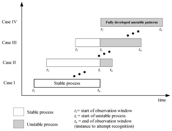
A critical distinction emerges in practical CCPR implementation, as shown in Figure 1, where online monitoring encounters four distinct cases. Case I occurs when a process is in a stable state, a common prerequisite for implementing online statistical process monitoring and recognition [7,8]. Case II represents the beginning of an unstable (deterioration) state. Attempting recognition at this stage could result in a high rate of false alarms and inaccurate classification due to insufficient unstable data [9,10]. Unstable patterns are often vaguely recognizable because they tend to appear as subsets of other patterns [11,12]. Case III would provide a clearer unstable pattern and is likely to lead to timely recognition and enable proactive process control [13]. Case IV represents the clearest unstable pattern, but it would be too late for preventive action and too risky for potentially catastrophic processes [14].

Figure 1. Possible cases for online recognition.

The onset of an unstable process (t_i) is normally unknown. For online real-time CCPR implementation, one should aim for Case III recognition since it promotes a balance between false alarms and delayed recognition [14]. Generally, Case III recognition is more difficult than Case IV because the patterns are still vague, incomplete, and dynamic [12,15].

The existing CCPR literature exhibits three substantive limitations that constrain its applicability to real-world quality control environments. First, the predominant focus on fully developed patterns (Case IV) significantly limits early-stage detection capability [16]. For example, Su et al. [17] employed an SVM trained on fully developed data, and Cheng et al. [18] proposed an end-to-end 1D convolutional neural network (1D CNN) with transfer learning to classify fully developed patterns. Chu et al. [19] also conducted a recognition study based on fully developed patterns that, despite incorporating adaptive feature selection, are fundamentally suited for offline recognition and are not directly applicable for early-stage detection or continuous online monitoring. This represents a critical research gap, as Tran et al. [20] encourage further work toward partially developed (online) CCPR systems to improve real-time adaptability. Cebeci and Simsir [21], Zan et al. [22], Unlu [23], and Ali et al. [24] emphasize the necessity of developing CCPR approaches capable of indicating process anomalies before they fully manifest as out-of-control signals.

Second, the methodological approaches employed for feature selection and network optimization in CCPR lack transparency and statistical rigor. Recent CCPR studies have increasingly adopted advanced neural network architectures such as convolutional neural networks (CNNs), long short-term memory (LSTM) networks, and hybrid models [25]. However, feature selection and network optimization traditionally rely on heuristic or meta-heuristic methods such as particle swarm optimization (PSO) and the bees algorithm. These meta-heuristic methods function as “black boxes”, offering limited interpretability regarding feature interactions, parameter significance, and the rationale underlying optimization decisions critical for quality engineers seeking to understand and validate system behavior on the shop floor.

Third, recent studies either lack essential industrial performance indicators such as Average Run Length (ARL₀, ARL₁) and Type I/II errors, or rely on offline evaluation using fully developed patterns [22,24], thereby addressing a less demanding problem than true online monitoring where instability onset is unknown.

This study addresses the above challenges in two complementary research objectives: (i) to identify a minimal yet discriminative statistical feature set specifically suited to partially developed patterns through fractional factorial design of experiments, and (ii) to optimize MLP network parameters using full factorial design of experiments. The effectiveness of the solution approach was evaluated under an online monitoring mechanism using industrial performance metrics (accuracy, Type I/II errors, ARL₀, ARL₁).

The remainder of this paper is organized as follows: Section 2 describes the methodology. Section 3 discusses input representation and statistical features. Section 4 presents the four-step recognizer development: preliminary parameter selection, minimal feature set selection, parameter fine-tuning, and online performance evaluation. Section 5 provides a discussion, and Section 6 concludes the paper.

2. Methodology

The investigation involved the generation of input data streams, recognizer design and testing, and performance measures. The coding for the investigation was performed using MATLAB’s Neural Network Toolbox (MathWorks, Natick, MA, USA).

2.1. Input Data Streams: The X-Bar Chart Patterns

Synthetic data generation through the Monte Carlo simulation method has become the standard approach for creating training datasets when real industrial data with sufficient abnormal patterns are unavailable. This methodology offers advantages including repeatability, controlled parameter variation, and the ability to generate diverse pattern examples with known truth labels. This study adopted this approach, in which process data streams were simulated using data generators as described by Swift [25]. The data generators are provided in Appendix A.1, and their parameters are as given in Table 1.

Table 1. Parameters used to generate process data.

Pattern Type	Parameters ($\mathit{\sigma }$)
Gradual increasing trend (TU)	Gradient: 0.015 to 0.025
Gradual decreasing trend (TD)	Gradient: −0.015 to −0.025
Sudden shift-up (SU)	Magnitude: 0.7 to 2.5
Sudden shift-down (SD)	Magnitude: −0.7 to −0.25
Cyclic (CYC)	Amplitude: 0.5 to 2.5; period = 10
Stable Process (NOR)	Mean = 0, SD = 1

The parameter values were varied uniformly between the above parameter limits to ensure the patterns were within $\pm$3$\sigma$. Random noise of 0.333$\sigma$ was added to all unstable patterns. Each set of data streams appeared in the observation window as ${\overline{x}}_1$,${\overline{x}}_2$, …, ${\overline{x}}_{20}$ where ${\overline{x}}_i={\displaystyle \frac{\sum _{i=1}^{n=5}{x}_i}{n}}$ (a sample of n = 5).

2.2. Recognizer Design and Testing

Traditional ANN models such as multi-layer perceptron (MLP) are still attractive and effective in CCPR studies [26]. MLP models have fewer parameters, making them easier to deploy in resource-constrained industrial settings. In this study, the recognizer was developed using a traditional multilayer perceptron (MLP) architecture, selected due to its simple, transparent, reliable, and practical nature as an alternative for quality engineers [27]. Its basic structure comprises an input layer, hidden layer(s), and an output layer. The size of the input vector dictates the size of nodes in the input layer. The number of nodes in the output layer was set according to the number of pattern classes (M = 6). The output node {O₁, O₂, …, O_M} with the maximum output value indicated the predicted class. The settings such as number of hidden layers, type of activation function, training stopping criteria, and error function were selected based on recommendations in the literature. However, the settings for the number of hidden nodes, training algorithm, and number of training samples were determined through experiments based on full factorial experimental design. More details are provided in Section 4.

2.3. Performance Measures

The recognizer performance was assessed using the established industrial performance metrics, namely recognition accuracy (ACC), Type I error ($\alpha$), Type II error ($\beta$), and Average Run Lengths (ARL₀, ARL₁). It is important for online applications to gauge ARL₀, which measures the average first time a recognizer generates a false alarm during a stable process [12]. A larger value of ARL₀ is better. ARL₁ measures how quickly an unstable pattern is recognized, where a smaller value indicates faster detection.

3. Input Representation and Statistical Features

Using features as input will result in a smaller network size and will generalize better than using raw observation data. This study adopted statistical features as investigated by Hassan et al. [28] since they were shown to be effective compared to the raw data stream representation. The statistical features were extracted from the data streams as presented in the observation moving window (w = 20). The mathematical expressions for statistical feature extraction are provided in Appendix A.2. The numerical values of these features varied widely, as they were measures of various statistical aspects of the data streams. The maximum and minimum values of the features were estimated from 30,000 sample patterns (5000 for each pattern type), and they are given in Table 2. ANN recognizer training is more efficient when the input vector falls within a certain range [29]. Thus, these values need to be normalized, for which Equation (1) was used.

$$P_n=2\times {\displaystyle \frac{(P-P_{min})}{(P_{max}-P_{min})}}-1$$

(1)

where: P_n = normalized observed feature values, P = observed feature values, P_min = minimum feature value, and P_max = maximum feature value. This step normalized the values to lie within [−1, 1].

Table 2. Maximum and minimum values of the statistical features.

Feature	Minimum Value (Pmin)	Maximum Value (Pmax)
Mean (MEAN)	9.55	10.44
Mean square value (MSV)	87.85	104.0
Skewness (SKEW)	−2.30	2.65
Slope (SLOPE)	−0.062	0.060
Kurtosis (KUR)	0.9	9.9
Standard deviation (STD)	0.067	0.450
Median (MEDIAN)	9.4	10.6
Range (RANGE)	0.21	1.56
Autocorrelation (ACOR)	0.0006	0.931
Cusum (CUS)	−7.1	7.1

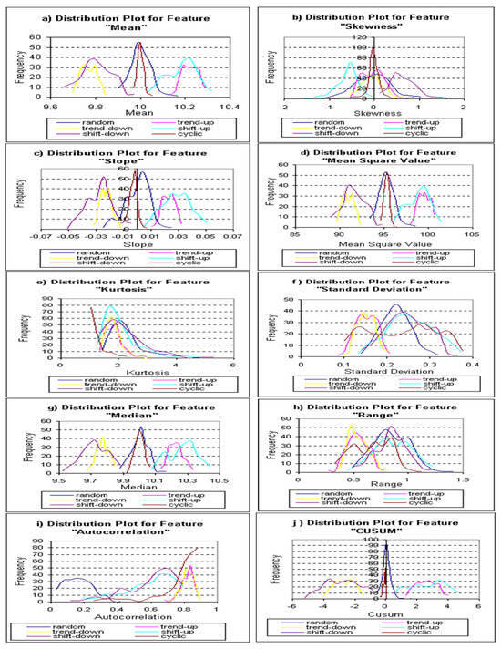
To assist in visualization, the features are plotted as frequency distributions, as shown in Figure 2.

Figure 2. Distribution plots for candidate features.

4. Design and Development of the Recognizer

The design and development of the MLP recognizer followed these steps:

• Step 1: Selection of preliminary MLP design and training parameters.
• Step 2: Selection of minimal feature set.
• Step 3: Fine-tuning design and training parameters for the recognizer.
• Step 4: Evaluation for online monitoring and recognition performance.

Traditional full and fractional factorial design of experiments (DOE) approaches were employed. The DOE design matrices provided quantifiable evidence and the significance of input features and recognizer parameter settings. To prevent the design matrices from becoming too large and resulting in heavily confounded results, we adopted an iterative experimental approach, using a full factorial design for MLP parameter selection and a fractional factorial design for selecting the minimum feature set.

4.1. Selection of Preliminary MLP Design and Training Parameters (Step 1)

As other parameters were common and established in the literature, we only investigated the settings for the number of hidden nodes (A), training algorithm (B), and training sample size (C), as shown in Table 3.

Table 3. Alternative parameter settings for ANN recognizer.

		Hidden Nodes (A)	Training Algorithm (B)	Training Sample Size (C)
Setting	Level −1	6	Adaptive back-propagation (traingdx)	2400
	Level +1	10	BFGS quasi-Newton back-propagation (trainbfg)	3888

Level −1 involved an MLP design with one hidden layer (six nodes), gradient descent with momentum and adaptive learning rate (traingdx), and 2400 training samples. The alternative setting (Level +1) involved 10 hidden nodes, BFGS quasi-Newton back-propagation (trainbfg), and 3888 training samples. For the hidden nodes, the distance between six and 10 nodes was deemed sufficient to demonstrate their effect. Both training algorithms traingdx and trainbfg aimed to minimize the loss (error) function of an MLP during training [30], but they differ in how they update weights [31]. Gradient descent (traingdx) uses only first-order derivatives, and BFGS quasi-Newton approximates second-order information (the curvature of the error surface) for faster convergence near minima. Meanwhile, the difference between 2400 and 3888 training samples should be sufficient to reveal its effects.

Table 4 provides the design matrix (full factorial 2³ matrix) and results of the recognition performance for 10 replicates of each run.

Table 4. Design matrix for factorial design and performance results.

	Parameters			Performance (% Correct)
Run	A	B	C	Mean	Std. Dev. (s)
1	−1	−1	−1	66.91	24.743
2	+1	−1	−1	82.53	4.290
3	−1	+1	−1	84.01	3.314
4	+1	+1	−1	85.34	4.305
5	−1	−1	+1	67.19	24.657
6	+1	−1	+1	76.08	20.914
7	−1	+1	+1	81.80	6.116
8	+1	+1	+1	85.03	4.062

The results in Table 4 show that the mean and standard deviation vary widely (mean: 66.91 to 85.34; s = 3.314 to 24.743). These results confirm that proper selection and combination of the design and training parameters are critical to the recognition performance. The findings suggested that run 4 (hidden nodes = 10, trainbfg, and training samples = 2400) (mean = 85.34, s = 4.305) and run 8 (hidden nodes = 10, trainbfg, and training samples = 3888) (mean = 85.03, s = 4.062) were among the best-performing runs.

4.2. Selection of Minimum Feature Set (Step 2)

In Step 2, a minimum feature set was selected using the MLP recognizer with 10 hidden nodes, BFGS algorithm (trainbfg), and 2400 training samples. Graphical plots in Figure 2 indicate that features MEDIAN and RANGE have discrimination ability among the patterns. However, these two features were excluded, as they seemed redundant with features MEAN and STD, respectively. Feature KUR (kurtosis) was also excluded, as the graphical plot indicated poor discriminative ability. SLOPE and ACOR were included, as the graphical plots showed reasonable discriminative ability and no obvious redundancies. In summary, the seven candidate features investigated for representing partially developed patterns were autocorrelation, cusum, mean, mean square value, skewness, standard deviation, and slope.

The minimum feature set selection was performed through experiments based on $2_{IV}^{7-2}$ fractional factorial experimental design [32]. The design matrix and the results for recognition performance (10 duplicates) are presented in Table 5. This design allocates seven candidate features (factors) and requires only 32 unique experimental runs. The design generators were F = ABCD and G = ABDE. In this design, all the main factors are free from any two-factor interactions, but a few of these factors are confounded with other two-factor interactions. This design matrix ensures that the features in each column are independent and free from confounding. The aliases for confounded two-factor interactions are CE + FG; CF + EG; and CG + EF. Interactions above two-factor were assumed negligible and treated as noise.

Table 5. Design matrix and performance results for the selection of feature set.

Run	ACOR	SKEW	STD	MSV	MEAN	CUS	SLOPE	Performance (% Correct)
	(A)	(B)	(C)	(D)	(E)	(F)	(G)	Mean	Std. Dev (s)
1	−1	−1	−1	−1	−1	+1	+1	49.13	12.60
2	+1	−1	−1	−1	−1	−1	−1	30.75	8.35
3	−1	+1	−1	−1	−1	−1	−1	30.29	6.15
4	+1	+1	−1	−1	−1	+1	+1	78.61	6.01
5	−1	−1	+1	−1	−1	−1	−1	62.96	12.47
6	+1	+1	−1	−1	−1	+1	+1	84.61	1.67
7	−1	+1	+1	−1	−1	+1	+1	67.02	8.82
8	+1	+1	+1	−1	−1	−1	−1	72.55	12.10
9	−1	−1	−1	+1	−1	−1	+1	25.98	1.76
10	+1	−1	−1	+1	−1	+1	−1	78.30	9.36
11	−1	+1	−1	+1	−1	+1	−1	72.80	4.04
12	+1	+1	−1	+1	−1	−1	+1	52.08	9.28
13	−1	−1	+1	+1	−1	+1	−1	70.60	7.11
14	+1	−1	+1	+1	−1	−1	+1	77.10	9.03
15	−1	+1	+1	+1	−1	−1	+1	70.21	8.00
16	+1	+1	+1	+1	−1	+1	−1	76.35	18.52
17	−1	−1	−1	−1	+1	+1	−1	65.45	4.09
18	+1	−1	−1	−1	+1	−1	+1	72.97	7.63
19	−1	+1	−1	−1	+1	−1	+1	56.63	15.71
20	+1	+1	−1	−1	+1	+1	−1	80.48	9.30
21	−1	−1	+1	−1	+1	−1	+1	63.77	7.12
22	+1	−1	+1	−1	+1	+1	−1	86.11	1.34
23	−1	+1	+1	−1	+1	+1	−1	17.92	24.18
24	+1	+1	+1	−1	+1	−1	+1	73.94	6.99
25	−1	−1	−1	+1	+1	−1	−1	62.73	17.85
26	+1	−1	−1	+1	+1	+1	+1	80.65	8.85
27	−1	+1	−1	+1	+1	+1	+1	65.93	14.50
28	+1	+1	−1	+1	+1	−1	−1	77.22	21.75
29	−1	−1	+1	+1	+1	+1	+1	72.19	13.32
30	+1	−1	+1	+1	+1	−1	−1	72.81	10.15
31	−1	+1	+1	+1	+1	−1	−1	66.16	7.21
32	+1	+1	+1	+1	+1	+1	+1	79.51	16.87

The feature-to-column assignment was made based on the findings of the preliminary design. Features that were perceived as more important were assigned to the left columns. Each experimental run was replicated 10 times to minimize the effect of random errors. Consequently, a total of 320 experiments (32 $\times$ 10) were conducted.

The results revealed that when all features were included as in standard order run 32, the performance was suboptimal (79.51%). Better performance was achievable with a reduced number of features, as indicated in run 6 (84.61%) and run 22 (86.11%). Since these were fractional experiments, analyzing the interactions among features was necessary.

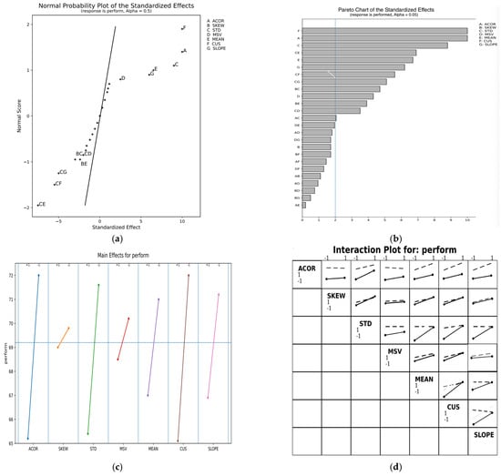
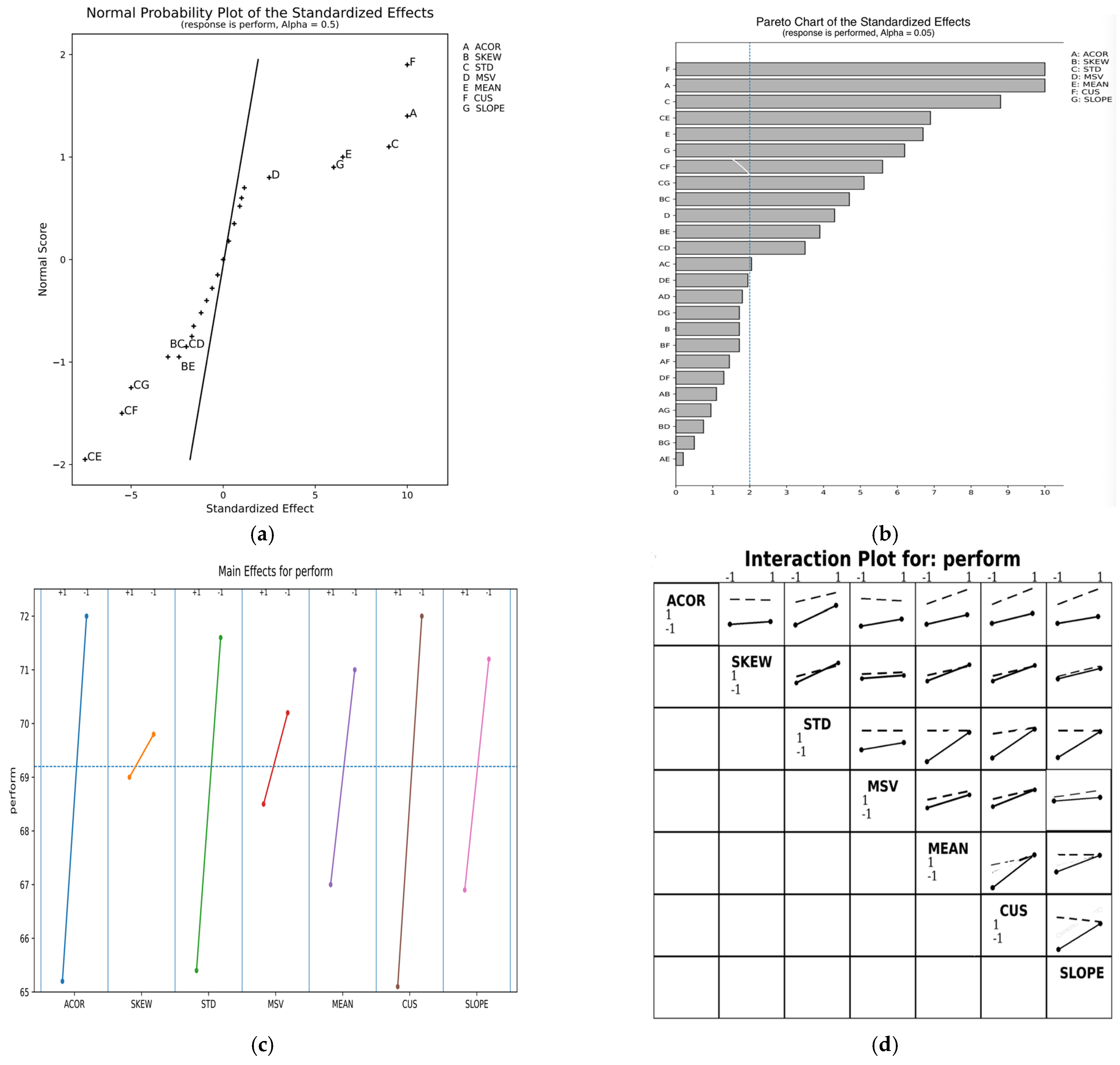
Analysis of variance (ANOVA) results indicated that both the main effects (F₀ = 53.85, p = 0.00) and two-way interactions (F₀ = 8.16, p = 0.00) were statistically significant. The linear regression model fitted satisfactorily with an insignificant lack of fit error (F₀ = 1.28, p = 0.265). Figure 3 shows the normal probability plot, Pareto chart, main effect plot, and interaction plots for the experimental results in Table 5.

Figure 3. Plots and chart for selection of feature set. (a) Normal probability plot of standardized effects. (b) Standardized effects. (c) Main effect. (d) Interaction plot.

At a significance level of α = 0.05, regression analysis indicated that features ACOR (p = 0.000), STD (p = 0.000), MSV (p = 0.005), MEAN (p = 0.000), CUS (p = 0.000), and SLOPE (p = 0.000) were significant. Additionally, the significant two-factor interactions were SKEW × STD (p = 0.001), SKEW × MEAN (p = 0.014), STD × MSV (p = 0.034), STD × MEAN (p = 0.000), STD × CUS (p = 0.000), and STD × SLOPE (p = 0.000). Table 6 summarizes the significant main and two-factor interaction effects (including aliases).

Table 6. Tentative significant main effects and interaction effects.

Main Effects	Interaction Effects and Aliases
ACOR	SKEW × MEAN
STD	SKEW × STD
MSV	STD × MSV
MEAN	STD × MEAN + CUS × SLOPE
SLOPE	STD × CUS + MEAN × SLOPE
CUS	STD × SLOPE + MEAN × CUS

The interaction plot in Figure 3 is important for interpreting and selecting other features. However, feature ACOR showed no interaction and was directly accepted without requiring reference to the interaction plot. As indicated by the solid response line in the SKEW × STD and SKEW × MEAN subplots (Figure 3), excluding feature skewness improved recognizer performance. From subplot STD × MSV, including both features STD and MSV resulted in a better response, as indicated by the dotted line. From the subplots (STD × MEAN + CUS × SLOPE), (STD × CUS + MEAN × SLOPE), and (STD × SLOPE + MEAN × CUS), the respective dotted lines did not support the exclusion of any of these features. On the other hand, the solid response lines for these subplots generally indicated that the exclusion of the respective first feature (row) resulted in a slightly lower response. Furthermore, the recognizer became more sensitive to changes in the second (column) features as indicated by the steeper solid line. This might be undesirable if changes in the levels of the second features were attributed to noise. The analysis suggests that it was more appropriate to include features STD, MEAN, CUS, SLOPE, MSV, and ACOR, and to exclude the insignificant feature SKEW. Confirmation experiments (30 replicates) resulted in average recognition accuracy of 85.52% (s = 2.832).

The selected feature set is conceptually appropriate for control chart pattern recognition because it captures the principal statistical characteristics, namely, location displacement, dispersion, cumulative deviation, directional change, signal energy, and temporal dependence. MEAN primarily reflects central level displacement and is therefore most sensitive to shift patterns, whereas STD measures within-window spread and is especially responsive to cyclic behavior due to the increased variability induced by oscillatory movement. CUSUM is particularly valuable under partially developed conditions because it accumulates weak but persistent deviations over time, making it highly sensitive to both shift and trend patterns even when their visual manifestation is still incomplete. In contrast, SLOPE directly represents the direction and magnitude of systematic change and thus serves as the strongest indicator of trend behavior. Meanwhile, MSV captures overall signal energy, which makes it useful for representing patterns such as shift and cycle. In addition, ACOR introduces a temporal dimension by quantifying serial dependence, thereby providing strong discrimination for cyclic patterns. Taken together, these features provide a compact yet complementary representation of process behavior, where discrimination does not rely on any single statistic in isolation but rather on their combined interaction. Specifically, shift patterns are most strongly represented by MEAN-CUSUM-MSV, trend patterns by SLOPE-CUSUM-ACOR, and cycle patterns by STD-ACOR-MSV. In contrast, random patterns do not exhibit a clear dominant feature profile, as their observations fluctuate irregularly without producing strong, persistent, directional, or periodic structure. This complementarity is especially important in Case III recognition, where patterns are only partially developed, and class boundaries remain highly overlapping. Thus, robust classification depends on integrating multiple statistical perspectives rather than relying on a single dominant feature.

4.3. Fine-Tuning ANN Design and Training Parameters (Step 3)

Considering the above minimal feature set, we confirm the effectiveness of the ANN parameter setting for feature selection. Ideally, this setting should be determined in the same experiment, but this would result in a large fractional experimental matrix, with low resolution (many confounded effects). As noted by Lawson [33], this challenge is normally addressed by performing serial experiments with clarification and technical judgment. This study adopted this approach. Ten replicate experiments were conducted using the minimum feature set identified in Section 4.2 to confirm the MLP parameters previously set as shown in Table 3.

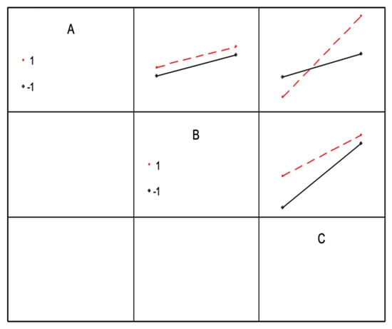
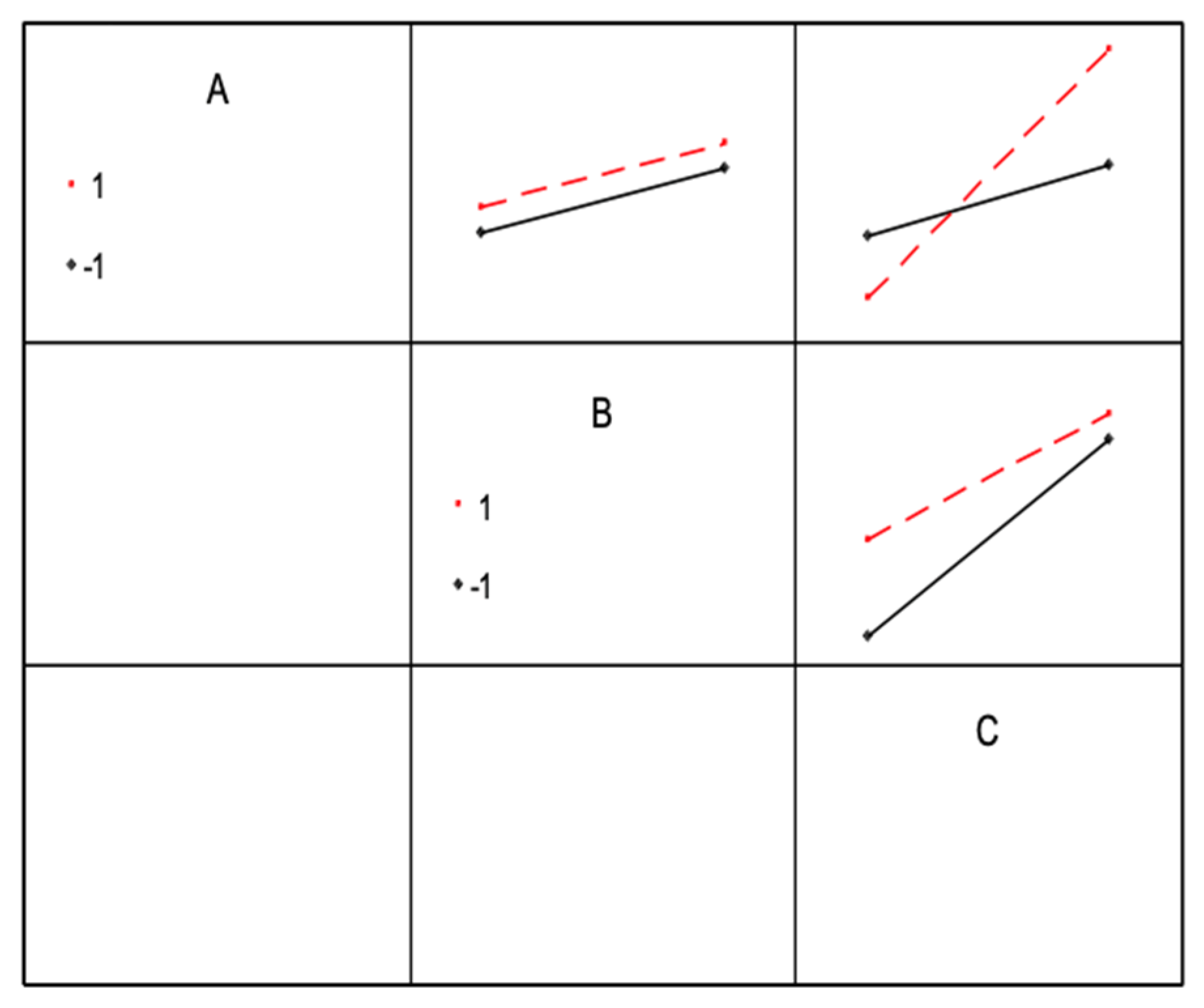
Regression analysis and ANOVA indicated that the number of training samples (C) was significant (p = 0.041). There was weak interaction (p = 0.26) between the number of hidden nodes (A) and the number of training samples (C). The interaction plots in Figure 4 confirm the best recognizer configuration comprised 10 hidden nodes (A⁺) trained with 3888 training samples (C⁺). This is indicated by the highest point (dotted line) in the interaction A × C. The best outcome was achieved in Run 8 of Table 7 (mean = 85.69, s = 4.025) using the BFGS quasi-Newton training algorithm (B⁺). We adopted this configuration for subsequent performance evaluations.

Figure 4. Interaction plots for the results of fine-tuning experiments.

Table 7. Design matrix and results of fine-tuning the ANN parameters.

	Parameters			Performance
Run	A	B	C	Mean	Std. Dev. (s)
1	−1	−1	−1	77.07	14.079
2	+1	−1	−1	76.22	13.261
3	−1	+1	−1	81.1	6.511
4	+1	+1	−1	83.27	8.488
5	−1	−1	+1	81.42	3.712
6	+1	−1	+1	83.84	4.737
7	−1	+1	+1	81.19	9.926
8	+1	+1	+1	85.69	4.025

The performance of the optimized recognizer and the selected feature set was evaluated using 1296 testing patterns (216 samples per class). Trend patterns (TU and TD) achieved the highest recognition rates, exceeding 92%. Cyclic patterns (CYC) approached 90% accuracy. Sudden (SU and SD) shift patterns showed lower performance, ranging from approximately 82 to 83%. The random pattern (RN) was the most difficult to recognize (78%). The overall average recognition accuracy was 86.1% (s = 2.21).

4.4. Online Recognition and Performance (Step 4)

To mimic real-time online situations, data streams were presented as observation points within a moving window (w = 20). All samples were initially stable processes and gradually deteriorated into unstable patterns. In real-time online process monitoring, data appear as continuous streams, where the onset of instability is unknown [34]. This study addressed this challenge with a serial monitoring and recognition approach. The overall online recognition procedure is presented in Algorithm 1. The recognizer was integrated with Nelson’s supplementary run rules first to assess process stability [35]. Details of Nelson’s supplementary run rules are provided in Appendix A.3. Only data streams identified as unstable were forwarded to the MLP recognizer, while stable streams continued without requiring recognition.

A classification decision was made when the maximum network output exceeded a threshold of 0.8; otherwise, monitoring continued to incorporate newer data into the moving window. The threshold was determined empirically to balance decision timing and accuracy. We observed that lower threshold values reduce rejections but increase premature (and potentially incorrect) classifications. Meanwhile, higher threshold values improve stringency but delay decisions. A value of 0.8 was selected to minimize forced misclassifications by favoring rejection (Reject Class) when patterns were inconclusive. The maximum number of recognition attempts was set to 20, which corresponds to the size of the moving window. If the recognition result remained inconclusive at the 20th attempt, the pattern was assigned to a reject class to avoid forced misclassification.

Algorithm 1. Online recognition procedure for partially developed X-bar chart patterns.

Input: Process data stream X (normalized); Decision thresholds; Maximum recognition iterations Nmax Output: Pattern classification $C \in \{Random, Trend, Shift,\dots \}$; Control action Initialization: Configure Recognizer: Multilayer Perceptron with 6 × 10 × 6 architecture Set activation functions: Hyperbolic tangent (tansig) for hidden layers and log-sigmoid for output layer Initialize iteration counter k = 0 Method: While do Data Acquisition and Feature Extraction:       Capture continuous process data streams.       Reduce input to a minimal feature set 2. Stability Evaluation:       If then             Continue monitoring.       Else             Repeat                  Execute Trained Recognizer to Predict Pattern Class:                       Output Yfinal = Max (O1, O2, …, OM)                       Increment k $\leftarrow k+1$                  Classification Logic:                       If (Yfinal is conclusive) then                            Identify Pattern C.                            If (C = Random) then                               Break Repeat and resume monitoring                            Else if (Yfinal > threshold) then                               Trigger Process Diagnosis.                               Implement Remedial Action                               Break Repeat and resume monitoring.                         Else if (k < Nmax) then                            Request additional process data samples                         Else                            Assign to “Reject Class” (unidentifiable pattern)                            Exit Loop.        Until (Final decision or k = Nmax)        End While

Table 8 summarizes the online performance, showing the percentage of correct, wrong, and reject classifications. The results suggest that pattern vagueness was more pronounced for Trends and Shift pattens, with sudden shift (27.3 to 32.7%) and gradual Trend patterns (19.5 to 24.7%) being classified as the Reject class due to inconclusive recognitions at 20th attempts. One possible reason was the limitation of run rules, which caused unstable patterns to be triggered too early (possibly in Case II). However, the recognizer was trained with patterns that were 75 to 90% developed (Case III).

Table 8. Online recognition performance (%).

	Recognition (%)
	Correct	Wrong	Reject
Random	86.2	11.3	2.5
Trend-up	72.8	7.7	19.5
Trend-down	66.8	8.5	24.7
Shift up	51.6	15.7	32.7
Shift-down	62.1	10.6	27.3
Cyclic	84.1	6.6	9.3
Average	70.6	10.1	19.3

For stable processes, 84.4% were correctly monitored by the run rules, while 15.6% were false alarms (Type I error), unnecessarily presented to the recognizer. Among the false alarms, only 1.8% were correctly recognized as random patterns (total RN = 86.2%). The remaining false alarms were either misclassified or assigned to the reject class. The experiment indicated that random patterns were challenging to recognize during the online recognition phase. For unstable processes, 97.5% were correctly detected by the run rules, yielding a Type II error of 2.5%. Compared to offline results (Section 4.3), recognition accuracy decreased when tested under online conditions. Trend patterns declined from above 92% (offline) to approximately 67–73% (online), while sudden shifts were reduced to approximately 52–62% (online). Cyclic patterns remained comparatively robust.

The online evaluation produced an average run length (ARL₀) for stable processes of 207.3 (s = 5.1) indicating a reasonable false alarm control. For unstable processes, the average recognition delay (ARL₁) was 10.86 (s = 0.08) observations. Overall, the results demonstrate that the MLP recognizer achieved stable monitoring performance, though recognition of abrupt shifts remains challenging in real-time environments. Gradual trend and cyclic patterns were more predictable due to their gradual nature.

5. Discussion

A central distinction in contemporary control chart pattern recognition research lies in the stage of pattern development targeted. Unlike most studies focusing on fully developed (offline) patterns, this work explicitly addresses partially developed patterns within a real-time monitoring paradigm, consequently increasing both problem complexity and practical relevance. This distinction is critical, as early-stage recognition operates under uncertainty, where signals are weak, evolving, and temporally ambiguous.

Only a limited number of recent works, notably Rojek et al. [1], Zan et al. [22], and Ünlü [23], attempted early-stage recognition. However, their contributions lack essential industrial performance indicators such as Average Run Length (ARL) and Type I/II errors, limiting applicability in real-world settings. Similarly, studies by Tayalati et al. [36] and Ali et al. [24], while claiming early detection, rely on offline evaluation using fully developed patterns, thereby addressing a less demanding problem. In contrast, this study adopts a true online monitoring paradigm, where instability onset is unknown. Table 9 summarizes the comparison with other studies.

Table 9. Comparison with other studies.

Study	Model	Pattern Stage	Accuracy (%)	Type I Error	Type II Error	ARL0	ARL1	Recognition Stage	Optimization
Zan et al. [22]	SECNN–BiLSTM	Partial	98.92	NR	NR	NR	NR	Early stage (Variable length)	Keras Tuner
Chu et al. [37]	Ensemble (BP, ELM, PNN, SVM)	Full	97.31	NR	NR	NR	NR	Limited (fully developed patterns)	Feature engineering
Rojek et al. [1]	Decision Tree	Full	Up to 100	NR	NR	NR	NR	Early stage	Parametric tuning
Ünlü [23]	ML + MRDS	Partial	~95	NR	NR	NR	NR	Early stage	Data simulation (Mix ratio)
Tayalati et al. [36]	LSTM-Autoencoder + SPC	Full	>95	Low	NR	NR	NR	Early stage (Pre-threshold)	Optimal threshold level
Ali et al. [24]	Wavelet + SVM	Full and partial	>96	1–6%	NR	NR	1.6–5.1	Early stage	Hybrid Signal decomposition
This Study	MLP (DOE-optimized)	Partial	86.1 (offline); 70.6 (online)	13.8%	2.5%	207.3	10.9	Early stage	DOE (factorial + fractional)

From a modeling perspective, the recent literature tends toward complex deep learning and hybrid architectures (e.g., SECNN–BiLSTM [22], LSTM-autoencoder hybrids [36], ensemble frameworks [24]). While these approaches reported high accuracies (often >95%), they typically require large datasets and extensive tuning and offer limited interpretability. Ünlü [23] employed an ML + MRDS (mixed ratio data simulation) modeling approach for early-stage pattern recognition. However, his work lacks evident transparency and online performance measures. Our study deliberately adopts a parsimonious MLP network, prioritizing transparency, computational efficiency, and deployability.

Performance comparison further highlights the importance of contextual evaluation. Although this study reports lower online accuracy (70.6%) compared to near-perfect accuracies in studies such as Chu et al. [37] (97.31%) and Rojek et al. [1] (up to 100%), these differences are largely attributable to the level of problem difficulty. Competing studies predominantly evaluate fully developed patterns with larger shifts, whereas the present work addresses incomplete, early-stage signals. Crucially, this study provides a comprehensive set of monitoring metrics (Type I = 13.8%, Type II = 2.5%, ARL₀ = 207.3, ARL₁ = 10.9) that are rarely reported across the literature. While Ali et al. [24] report superior performance metrics particularly for Type I error and ARL₁, their results are obtained under less stringent experimental conditions. Specifically, they focused primarily on detecting process shifts and outliers and restricted their simulations to process variability levels of σ = 1 and σ = 2σ. In contrast, the present study considers a broader range of process shifts and patterns, as summarized in Table 1. Furthermore, Ali et al. [24] conducted simulations using subgroup sizes of n = 5 and n = 10, whereas the present study uses only n = 5. The higher Type I error observed in our study reflects a trade-off to enable earlier detection, while the low Type II error confirms strong sensitivity to true process shifts.

A key methodological contribution lies in the structured feature selection strategy using DOE. Unlike heuristic or metaheuristic approaches, which often function as black boxes, the DOE approach enables statistically interpretable feature reduction, yielding a minimal yet effective set (mean, standard deviation, autocorrelation, slope, mean square value, and CUSUM). Each feature captured complementary process dynamics. This transparency strengthens practitioner trust and facilitates industrial adoption. The two-stage optimization approach combining full factorial design for model parameters and fractional factorial design for feature selection provides quantifiable insight.

Importantly, this study integrates pattern recognition within an online monitoring system, addressing a gap often overlooked in prior work. By combining Nelson’s rules for stability assessment with an MLP-based classifier, the proposed approach ensures that recognition is only performed when instability is detected. In summary, while state-of-the-art studies emphasize algorithmic sophistication and high offline accuracy, this study contributes a balanced, application-oriented approach characterized by

• Statistically grounded feature and parameter optimization
• Comprehensive performance evaluation
• Real-time applicability
• Interpretability and deployment feasibility

This study has specific constraints that limit generalizability of its results. Its reliance on simulated datasets may not fully capture the complexity of real industrial process variability and noise conditions encountered in actual manufacturing environments. Additionally, this study addressed partially developed patterns within a fixed observation window (w = 20), which presents specific challenges not fully generalizable across different window sizes. Another limitation is that the recognizer demonstrated difficulty with early-stage sudden shift patterns (SU/SD), achieving only 52–62% online recognition accuracy for these patterns. This is possibly due to the temporal dynamics of abrupt changes not being adequately captured within the current model. Furthermore, the Type I error rate of 13.8% might have been influenced by the limitation of Nelson’s supplementary run rules. Possibly, the rules were triggering instability detection at Case II (beginning of deterioration) rather than the intended Case III (clearer unstable pattern).

6. Conclusions

This study contributes to the CCPR literature by shifting the focus from high-accuracy offline classification toward practical early-stage recognition. The integration of DOE-based optimization, transparent feature selection, and comprehensive performance evaluation positions this work at the intersection of statistical process control and machine learning. The study demonstrates a challenging online performance with 70.6% accuracy, representing realistic expectations for early-stage recognition, providing critical guidance for practitioners intending to implement CCPR systems.

The paper implemented statistical design of experiments for both network parameter optimization and feature selection. Through fractional factorial experiments, a minimal yet discriminative statistical feature set comprising autocorrelation, mean, mean-square value, standard deviation, slope, and cumulative sum was derived. The study confirmed that recognition performance is highly sensitive to the selection of the feature set, number of hidden nodes, training algorithm, and training sample size.

Future research should prioritize validation using real industrial process datasets to assess whether the proposed approach maintains performance under domain-specific variability and noise conditions. Second, addressing the recognized difficulty with early-stage sudden shift patterns represents a critical research opportunity. This could involve investigating hybrid architectures to better capture temporal dynamics of abrupt changes or exploring alternative window sizes and temporal representations. Third, improving the stability detection methodology beyond Nelson’s supplementary run rules is essential. Finally, conducting sensitivity analysis on the decision threshold and the reject class mechanism under varying noise conditions would provide more robust outcomes.

Appendix A.1. Formula for Data Generators

Consider the following notations:

μ = mean of the process when it is in-control

${\sigma }_{\stackrel{\_\_}{x}}$ = process standard deviation when the process is in-control

$X_t$ = individual process data (quality measurement) at time t

$\stackrel{\_\_}{X_t}$ = average of quality measurements (subgroup average) at time t

t = time of sampling

t₀ = a time reference point

Z_t = standard normal random variate at time t: N(0,1)

s = slope of the trend pattern

b = baseline noise level (magnitude of random noise)

h = magnitude of process shift

n = sample size (subgroup size)

c₁, c₂ = amplitudes of the cyclic pattern

T = period of the cyclic pattern.

The individual process data for various types of unnatural patterns were simulated based on the following process models:

(a) In-control data (random pattern)

$$X_t=\mu +(b{Z}_t {\sigma }_{\stackrel{\_}{x}})$$

(b) Trend pattern

$$X_t=\mu +s (t-t_0) {\sigma }_{\stackrel{\_}{x}}+(b Z_t {\sigma }_{\stackrel{\_}{x}}) (\mathrm{upward} \mathrm{trend})$$

$$X_t=\mu -s (t-t_0) {\sigma }_{\stackrel{\_}{x}}+(b Z_t {\sigma }_{\stackrel{\_}{x}}) (\mathrm{downward} \mathrm{trend})$$

(c) Shift pattern

$$X_t=\mu +(h{\sigma }_{\stackrel{\_}{x}})+(b Z_t {\sigma }_{\stackrel{\_}{x}}) (\mathrm{upward} \mathrm{shift})$$

$$X_t=\mu -(h{\sigma }_{\stackrel{\_}{x}})+(b Z_t {\sigma }_{\stackrel{\_}{x}}) (\mathrm{downward} \mathrm{shift})$$

(d) Cyclic pattern

$$X_t=\mu + (b Z_t {\sigma }_{\stackrel{\_}{x}}) + c_1{\sigma }_{\stackrel{\_}{x}} \cos \left[{\displaystyle \frac{2\pi (t-t_0)}{T}}\right]+{\mathrm{c}}_2{\sigma }_{\stackrel{\_}{x}} \sin \left[{\displaystyle \frac{2\pi (t-t_0)}{T}}\right]$$

The subgroup averages for all the above individual data were obtained as follows: $\stackrel{\_}{X_t}={\displaystyle \frac{{\displaystyle \sum _{t=1}^n{X}_t}}{n}}$, where n is the subgroup size.

Appendix A.2. Formula for Feature Extraction

The mathematical expressions for extracting statistical features Mean, Median, Standard Deviation, and Range are widely available in most of the texts on SPC or statistics. The mathematical expressions for extracting the rest of the statistical features are as follows:

(a) Mean square value (MSV)

$$\widetilde{x^2}={\displaystyle \frac{x_0^2+x_1^2+x_2^2+\dots +x_N^2}{N+1}}={\displaystyle \frac{1}{N+1}}{\displaystyle \sum _{i=0}^N{x}_i^2}$$

(b) Cumulative sum (CUSUM)

The tabular CUSUM provides accumulated deviations from a target value ${\mu }_0$ that are above the target, with statistic C⁺ and accumulated deviations from ${\mu }_0$ that are below the target with C⁻ statistic. The statistics C⁺ and C⁻, which represent one-sided upper and lower cumulative sums, are computed as follows:

$$C_i^{+}= \max [0, x_i - ({\mu }_0+ K) + C_{i-1}^{+}]$$

$$C_i^{-}=\max [0, ({\mu }_0-K)-x_i+C_{i-1}^{-}]$$

where the starting values are $C_0^{+}=C_0^{-}=0$.

The last CUSUM statistic for each data stream was taken as the representative feature. The reference value, K, was set to 0.5 shift magnitude to provide sensitivity to detect shift of 1$\sigma$.

(c) Skewness

Skewness (a₃) provides information concerning the shape of the distribution. It indicates a lack of symmetry in the data distribution. Skewness of a frequency distribution is given by

$$a_3={\displaystyle \frac{{\displaystyle \sum _{i=1}^h{f}_i{\left(X_i-\stackrel{\_}{X}\right)}^3}/n}{s^3}}$$

where:

n = the number of observed values

s = sample standard deviation

f_i = frequency in a cell or of an observed value

$\stackrel{\_}{X}$ = average of the observed value

X_i = observed value.

(d) Kurtosis

Kurtosis (a₄) is the peakedness of the data. Similarly to skewness, kurtosis provides information concerning the shape of the distribution. The kurtosis value is used as a measure of the height of the peak in a distribution:

$$a_4={\displaystyle \frac{{\displaystyle \sum _{i=1}^h{f}_i{\left(X_i-\stackrel{\_}{X}\right)}^4}/n}{s^4}}$$

(e) Slope

$\stackrel{\_}{Y}$ denotes the mean of Y_i and $\stackrel{\_}{X}$ denotes the mean of X_i of the (X_i, Y_i) pairs of sample observations. The best-fitting straight line is given by Y_i = b₀ + b₁X_i, where b₁ is the slope. The least-squares line and the slope are obtained as follows:

$$\widehat{{\displaystyle Y}}=\widehat{{\beta }_0}+\widehat{{\beta }_1}X$$

$$\widehat{{\beta }_1}={\displaystyle \frac{{\displaystyle \sum _{i=1}^n\left(X_i-\stackrel{\_}{X}\right)}\left(Y_i-\stackrel{\_}{Y}\right)}{{\displaystyle \sum _{i=1}^n{\left(X_i-\stackrel{\_}{X}\right)}^2}}}$$

$$\widehat{{\beta }_1}={\displaystyle \frac{{\displaystyle \sum _{i=1}^n{X}_i{Y}_i}-\left({\displaystyle \sum _{i=1}^n{X}_i}\right)\left({\displaystyle \sum _{i=1}^n{Y}_i}\right)/n}{{\displaystyle \sum _{i=1}^n{X_i}^2-{\left({\displaystyle \sum _{i=1}^n{X}_i}\right)}^2/n}}}$$

$$\widehat{{\beta }_0}=\stackrel{\_}{Y}-\widehat{{\beta }_1}\stackrel{\_}{X}$$

The intercept is given by $\widehat{{\beta }_0}$, and $\widehat{{\beta }_1}$ is the slope of the fitted line. The value of $\widehat{{\beta }_1}$ was used as the feature in this study.

(f) Average autocorrelation

Autocorrelation exists when one part of a signal depends on another part of the same signal. It measures the dependence of data at one instant in time on another instant in time. A signal will show the greatest fluctuations with time if there is no correlation between any two neighboring values. For random signals, one can expect that its value in the distant future would be negligibly dependent upon its present value.

The autocorrelation function is defined as follows:

$$R_{xx}\left[k\right]\cong {\displaystyle \frac{1}{N+1-k}}\left[x_0{x}_k+x_1{x}_{1+k}+\dots x_{N-k}{x}_N\right]$$

where N is the number of observations, and k is the lag. In this study, the average values for autocorrelation at lags 1 and 2 were used as the feature. These lags were chosen based on preliminary simulation runs.

Appendix A.3. Nelson’s Run Rules for Stability Tests

Table A1. Nelson’s run rules [35].

Test No.	Run Rules
Test 1	One or more points outside the control limit
Test 2	Nine consecutive points are on the same side of the central line
Test 3	Six points in a row steadily increasing or decreasing
Test 4	Fourteen points in a row alternating up and down
Test 5	Two out of three consecutive points on the same side of the central line are between 2$\sigma$ and the control limits
Test 6	Four out of five consecutive points are between 1$\sigma$ and the control limit on the same side of the central line
Test 7	Fifteen consecutive points are between −1$\sigma$ and +1$\sigma$
Test 8	Eight consecutive points are on both sides of the central line, with none within −1$\sigma$ and +1$\sigma$

Table A1. Nelson’s run rules [35].

Test No.	Run Rules
Test 1	One or more points outside the control limit
Test 2	Nine consecutive points are on the same side of the central line
Test 3	Six points in a row steadily increasing or decreasing
Test 4	Fourteen points in a row alternating up and down
Test 5	Two out of three consecutive points on the same side of the central line are between 2$\sigma$ and the control limits
Test 6	Four out of five consecutive points are between 1$\sigma$ and the control limit on the same side of the central line
Test 7	Fifteen consecutive points are between −1$\sigma$ and +1$\sigma$
Test 8	Eight consecutive points are on both sides of the central line, with none within −1$\sigma$ and +1$\sigma$

References

- Rojek, I.; Kujawińska, A.; Burduk, R.; Mikołajewski, D. Improving process control through decision tree-based pattern recognition. Electronics 2024, 13, 4823. [Google Scholar] [CrossRef] [Scilit]
- Masood, I.; Shyen, V.B.E. Quality control in hard disk drive manufacturing using pattern recognition technique. IOP Conf. Ser. Mater. Sci. Eng. 2016, 160, 012008. [Google Scholar] [CrossRef] [Scilit]
- Appollis, L.-L.M.; van Dyk, W.A.; Matope, S. Using failure modes and effects analysis as a problem-solving guideline when implementing SPC in a South African chemical manufacturing company. S. Afr. J. Ind. Eng. 2020, 31, 1. [Google Scholar] [CrossRef] [Scilit]
- Niemietz, P.; Fencl, M.; Bergs, T. Study on learning efficient stroke representations in clocked sheet metal processing: Theoretical and practical evaluation. Prod. Eng. 2023, 17, 279. [Google Scholar] [CrossRef] [Scilit]
- Biesterfield, D.H. Quality Control, 9th ed.; Pearson: Boston, MA, USA, 2012. [Google Scholar]
- Guh, R.-S.; Zorriassatine, F.; Tannock, J.D.T.; O’Brien, C. Online control chart pattern detection and discrimination: A neural network approach. Artif. Intell. Eng. 1999, 13, 413–425. [Google Scholar] [CrossRef] [Scilit]
- Thor, J.; Lundberg, J.; Ask, J.; Olsson, J.; Carli, C.; Härenstam, K.P.; Brommels, M. Application of statistical process control in healthcare improvement: Systematic review. BMJ Qual. Saf. 2007, 16, 387. [Google Scholar] [CrossRef] [Scilit] [PubMed]
- Simion, C. Assessment of process stability and capability in a manufacturing organization: A case study. MATEC Web Conf. 2021, 343, 05011. [Google Scholar] [CrossRef] [Scilit]
- Teoh, W.L.; Le, G.K.; Chong, Z.L.; Chew, X.; Lee, M.H.; Khaw, K.W. Optimizing variable sample size chart through median run length with estimated process parameters. Sains Malays. 2025, 54, 1187. [Google Scholar] [CrossRef] [Scilit]
- Santarisi, N.; Barghash, M.A.; Barghash, A. A multi-stage ensemble neural network for accurate differentiation between false and real alarms in quality control charts. Int. J. Intell. Eng. Syst. 2022, 15, 150. [Google Scholar] [CrossRef] [Scilit]
- Pelegrina, G.D.; Duarte, L.T.; Jutten, C. Blind source separation and feature extraction in concurrent control charts pattern recognition: Novel analyses and comparison. Comput. Ind. Eng. 2015, 92, 105. [Google Scholar] [CrossRef] [Scilit]
- Hachicha, W.; Ghorbel, A. A survey of control-chart pattern-recognition literature (1991–2010). Comput. Ind. Eng. 2012, 63, 204. [Google Scholar] [CrossRef] [Scilit]
- Farissi, O.E.; Moudden, A. Application of neuro-fuzzy in the recognition of control chart patterns. Int. J. Comput. Appl. 2017, 166, 29. [Google Scholar] [CrossRef] [Scilit]
- García, E.; Peñabaena-Niebles, R.; Percybrooks, W.; Palomino, K. A novel methodology for performance evaluation in advanced quality control. Mathematics 2025, 13, 259. [Google Scholar] [CrossRef] [Scilit]
- Cheng, C.; Chen, P.-W.; Hsieh, Y.; Wu, Y. Multivariate process control chart pattern classification using multi-channel deep convolutional neural networks. Mathematics 2023, 11, 3291. [Google Scholar] [CrossRef] [Scilit]
- Gutiérrez, H.; Pham, D. Estimation and generation of training patterns for control chart pattern recognition. Comput. Ind. Eng. 2016, 90, 502–513. [Google Scholar] [CrossRef] [Scilit]
- Su, C.-J.; Chen, I.-F.; Tsai, T.-R.; Wang, T.-H.; Lio, Y. Support vector machines and model selection for control chart pattern recognition. Mathematics 2025, 13, 592. [Google Scholar] [CrossRef] [Scilit]
- Cheng, C.-S.; Ho, Y.; Chiu, T.-C. End-to-end control chart pattern classification using a 1D convolutional neural network and transfer learning. Processes 2021, 9, 1484. [Google Scholar] [CrossRef] [Scilit]
- Chu, H.; Zhao, K.; Cheng, Q.; Li, R.; Yang, C. Control chart patterns recognition based on optimized deep belief neural network. IEEE Access 2020, 8, 203685–203699. [Google Scholar] [CrossRef] [Scilit]
- Tran, P.H.; Nadi, A.A.; Nguyen, T.H.; Tran, K.D.; Tran, K.P. Application of machine learning in statistical process control charts: A survey and perspective. In Control Charts and Machine Learning for Anomaly Detection in Manufacturing; Springer: Cham, Switzerland, 2021. [Google Scholar] [CrossRef] [Scilit]
- Cebeci, U.; Şimşir, U. Adaptive statistical process control by managing uncertainty in process monitoring. Artif. Intell. Theory Appl. 2025, 5, 11–32. [Google Scholar]
- Zan, T.; Jia, X.; Guo, X.; Wang, M.; Gao, X.; Gao, P. Variable-length control chart pattern recognition using SECNN-BiLSTM. Sci. Rep. 2025, 15, 5921. [Google Scholar] [CrossRef] [Scilit]
- Ünlü, R. A robust data simulation technique to improve early detection performance of a classifier in control chart pattern recognition systems. Inf. Sci. 2021, 553, 188–204. [Google Scholar] [CrossRef] [Scilit]
- Ali, T.; Taha, H.; Sedeeq, B.; Hayawi, H. An innovative hybrid control chart combining wavelet decomposition and support vector machine for effective outlier detection. Front. Appl. Math. Stat. 2025, 11, 1682448. [Google Scholar] [CrossRef] [Scilit]
- Swift, J.A. Development of a Knowledge-Based Expert System for Control Chart Pattern Recognition Analysis. Ph.D. Thesis, Oklahoma State University, Stillwater, OK, USA, 1987. [Google Scholar]
- Chang, S.I.; Ghafariasl, P. A review of artificial intelligence impacting statistical process monitoring and future directions. arXiv 2025, arXiv:2503.01858. [Google Scholar] [CrossRef] [Scilit]
- Tercan, H.; Meisen, T. Machine learning and deep learning based predictive quality in manufacturing: A systematic review. J. Intell. Manuf. 2022, 33, 1879. [Google Scholar] [CrossRef] [Scilit]
- Hassan, A.; Baksh, M.S.N.; Shaharoun, A.M.; Jamaluddin, H. Improved SPC chart pattern recognition using statistical features. Int. J. Prod. Res. 2003, 41, 1587–1603. [Google Scholar] [CrossRef] [Scilit]
- Beale, M.H.; Hagan, M.T.; Demuth, H.B. Neural Network Toolbox User’s Guide; MathWorks: Natick, MA, USA, 2015. [Google Scholar]
- Hammad, M.M. Artificial neural network and deep learning: Fundamentals and theory. arXiv 2024, arXiv:2408.16002. [Google Scholar] [CrossRef] [Scilit]
- Taghavifar, H.; Mardani, A. Application of artificial neural networks for prediction of traction performance parameters. J. Saudi Soc. Agric. Sci. 2013, 13, 35. [Google Scholar] [CrossRef] [Scilit]
- Montgomery, D.C. Design and Analysis of Experiments, 10th ed.; Wiley: Hoboken, NJ, USA, 2020. [Google Scholar]
- Lawson, J. Comparison of conditional main effects analysis in fractional factorial experiments. Qual. Reliab. Eng. Int. 2020, 36, 1454. [Google Scholar] [CrossRef] [Scilit]
- Wilhelm, Y.; Schreier, U.; Reimann, P.; Mitschang, B.; Ziekow, H. Data science approaches to quality control in manufacturing: A Review of Problems, Challenges and Architecture. Commun. Comput. Inf. Sci. 2020, 45, 45–65. [Google Scholar] [CrossRef] [Scilit]
- Nelson, L.S. The Shewhart control chart tests for special causes. J. Qual. Technol. 1984, 16, 237–239. [Google Scholar] [CrossRef] [Scilit]
- Tayalati, F.; Boukrouh, I.; Bouhsaien, L.; Azmani, A.; Azmani, M. Hybrid approach integrating deep learning-autoencoder with statistical process control chart for anomaly detection. IEEE Access 2024, 12, 95576–95598. [Google Scholar] [CrossRef] [Scilit]
- Chu, H.; Dong, Y.; Cheng, Q.; Yan, J.; Zhao, Y.; Cao, J.; Zhang, C.; Chen, X. Pattern recognition of control charts based on data feature enhancement and ensemble learning of classifiers for dimensional accuracy of products. Int. J. Prod. Res. 2024. [Google Scholar] [CrossRef] [Scilit]
Disclaimer/Publisher’s Note: The statements, opinions and data contained in all publications are solely those of the individual author(s) and contributor(s) and not of MDPI and/or the editor(s). MDPI and/or the editor(s) disclaim responsibility for any injury to people or property resulting from any ideas, methods, instructions or products referred to in the content. |
© 2026 by the author. Licensee MDPI, Basel, Switzerland. This article is an open access article distributed under the terms and conditions of the Creative Commons Attribution (CC BY) license.