On the Numerical Reliability of Lyapunov-Based Chaos Analysis in Optically Injected Semiconductor Lasers: A Phasor-Quadrature Comparison

Abstract

Lyapunov-exponent-based diagnostics are widely used to quantify deterministic chaos in optically injected semiconductor lasers (OISLs). In most numerical implementations, the optical field is represented either in phasor coordinates $(A,\psi ,N)$ or in Cartesian quadrature coordinates $(X,Y,N)$. Although these representations are mathematically related through a smooth coordinate transformation away from vanishing field amplitude, their numerical realizations can exhibit markedly different robustness in variational calculations, directly impacting the reliability of Lyapunov exponent estimation and chaoticity maps. In this work, we present a systematic assessment of the numerical reliability of Lyapunov-based chaos analysis in master-slave optically injected semiconductor lasers using both phasor and quadrature formulations. The full Lyapunov spectrum was computed via a noise-free variational method that integrates the nonlinear dynamics together with the corresponding Jacobian equations using a fourth-order Runge-Kutta scheme combined with periodic QR orthonormalization. High-resolution Lyapunov maps were constructed in the injection strength-frequency detuning parameter space, and the consistency between both formulations was quantitatively evaluated. While both approaches reproduce the overall structure of chaotic and non-chaotic regions, the phasor formulation may generate spurious positive Lyapunov exponents in regimes where the optical field amplitude approaches low values. These discrepancies originate from singular terms proportional to $1/A$ and $1/A^2$ in the variational Jacobian of the phasor model, which can lead to numerical amplification and artificial chaotic signatures. The quadrature formulation avoids these singularities and provides numerically stable and physically consistent Lyapunov spectra across the explored parameter space. The results establish practical guidelines for robust chaos quantification in optically injected semiconductor lasers and highlight the importance of representation choice in variational Lyapunov analysis of nonlinear photonic systems.

1. Introduction

Chaotic systems are defined by deterministic nonlinear equations that exhibit sensitive dependence on initial conditions, broadband spectral signatures, and a coexistence of order and unpredictability. Their simplicity at the equation level belies the richness of the resulting trajectories, enabling a wide range of applications that exploit chaos as a functional resource. Chaos-based encryption, for example, leverages the inherent unpredictability and sensitivity of chaotic signals to construct cryptographic schemes that are resistant to brute-force and differential attacks while remaining computationally efficient.

Recent years have seen rapid advances in the design and application of high-dimensional and hyperchaotic systems for secure information processing and hardware-oriented implementations. Fractional-order and state-dependent hyperchaotic systems have been proposed for high-performance image encryption and secure data transmission, demonstrating enhanced sensitivity to initial conditions and large key spaces suitable for modern security requirements. Parallel developments in memristive and neural network-based chaotic systems further illustrate the breadth of current research. Memristive neural networks have demonstrated complex chaos-driven behaviors with implications for secure computing [1,2], while fractional-order Hopfield networks and modular logistic-map-based systems have been explored for efficient and robust chaotic image protection [3,4]. In addition, multiscroll and memristor-based neural architectures have enabled compact hardware realizations of complex chaotic dynamics, including FPGA implementations capable of real-time operation and synchronization.

These developments collectively underscore the growing demand for physically realizable chaotic sources that combine broadband dynamics, robustness, and controllability. Within this broader context, optically injected semiconductor lasers provide a particularly attractive platform due to their intrinsic high-speed carrier-photon dynamics and compatibility with integrated photonic technologies, enabling deterministic generation of high-bandwidth chaos suitable for next-generation secure communication and photonic information-processing systems. As integrated photonics evolves, chip-scale implementations of chaotic semiconductor lasers continue to improve in performance and practicality [5], enabling compact and energy-efficient secure communication systems [6] and contributing to the advancement of AI and quantum photonic technologies [7].

The field of chaos-based optical communication has likewise advanced significantly, transitioning from isolated demonstrations to practical, high-capacity transmission systems. Spitz et al. demonstrated private communication using quantum-cascade-laser chaos [8]; Xie et al. realized 100 Gb/s chaotic coherent communication over 800 km [9]; and Wang et al. demonstrated high-speed secure transmission over 130 km multi-core fibers using mutually injected semiconductor lasers [10]. Subsequent breakthroughs include 256 Gb/s chaotic communication over 1600 km [11], 100 Gb/s secure communication over 100 km using wideband chaotic lasers [12], and chaos synchronization over 8190 km [13], underscoring the growing maturity of chaos-enabled photonic networks. Chaotic signal generation in optically injected semiconductor lasers (OISLs) has become a central topic in nonlinear photonics, providing compact and high-speed platforms for the exploration and exploitation of complex dynamical behavior [7].

In the standard master-slave configuration, the dynamical response of the slave laser depends primarily on the injection strength and frequency detuning, leading to stable injection locking, periodic oscillations, quasi-periodicity, and deterministic chaos [14]. The nonlinear dynamics of such systems have been extensively characterized through bifurcation analysis and stability studies in recent decades.

While bifurcation-based approaches provide a comprehensive qualitative description of OISL dynamics [15], quantitative characterization of chaos based on Lyapunov exponents has become increasingly important for both fundamental studies and technological applications. In particular, Lyapunov exponents provide a rigorous metric for distinguishing chaotic, periodic, and quasi-periodic regimes and are widely used in applications such as secure optical communications [16,17], random number generation [18,19,20], microwave photonics [21], and neuromorphic or reservoir computing platforms [22]. The reliability and reproducibility of Lyapunov-based chaos diagnostics are therefore of fundamental importance.

Recent progress in chaos-enabled photonic systems has emphasized the importance of controlled and broadband chaotic emission in optically injected semiconductor lasers. For instance, Huang et al. demonstrated a parallel wideband chaos generation system based on an integrated array of distributed feedback lasers with intensity-modulated optical injection, achieving multi-channel chaotic signals with bandwidths exceeding 30 GHz and enabling high-throughput photonic information processing and random bit generation [23]. In related work, Huang et al. reported wideband chaos generation using a VCSEL with intensity-modulated optical injection for high-rate physical random number generation, highlighting the role of injection parameters and dynamical stability in determining chaos quality and bandwidth [24]. Efforts to stabilize chaos and mitigate intermittency have also been reported [25], further cementing the role of chaotic semiconductor lasers in secure photonic information processing. These recent studies illustrate the growing technological relevance of optically injected laser chaos and reinforce the need for formulation-independent and numerically reliable methods for quantifying deterministic chaotic dynamics. The present work addresses this need by providing a systematic and reproducible Lyapunov-based analysis framework and by demonstrating the numerical equivalence and reliability of phasor and quadrature formulations for chaos characterization.

In most Lyapunov-based studies of optically injected semiconductor lasers, the optical field is represented using a phasor formulation in terms of amplitude and phase variables $(A,\psi ,N)$. An alternative representation employs Cartesian quadrature variables $(X,Y,N)$, where the optical field is decomposed into its real and imaginary components. Although these two formulations are mathematically equivalent and related by a smooth coordinate transformation away from vanishing field amplitude, their numerical implementations can exhibit markedly different robustness when used for variational Lyapunov analysis.

In particular, the phasor formulation introduces terms proportional to $1/A$ and $1/A^2$ in the variational Jacobian. When the system trajectory evolves through low-amplitude regions of phase space, a situation that frequently arises in chaotic regimes, these terms may lead to numerical amplification and affect the stability of Lyapunov exponent estimation. Despite the extensive literature on OISL dynamics, the numerical reliability of Lyapunov-based chaos quantification for different coordinate representations has not been systematically examined.

To ensure internal consistency of the rate-equation normalization used in this work, particular attention was given to the equilibrium field amplitude of the solitary slave laser. A previously overlooked factor of two in the steady-state field normalization can lead to a systematic discrepancy in the analytical estimation of the relaxation-oscillation frequency. By correcting this normalization and computing the relaxation frequency directly from the eigenvalues of the Jacobian evaluated at the free-running equilibrium, we obtain a self-consistent reference frequency derived from the same dynamical system used in the Lyapunov analysis. For the parameter set considered here, this procedure yields a relaxation frequency of approximately $7.58$ GHz. Although this correction does not alter the qualitative structure of the chaos maps, it ensures physical transparency and parameter consistency throughout the analysis.

While periodic, quasi-periodic, and chaotic regimes in standard OILs are well known [14,26,27,28], the numerical reliability of chaos quantification for different coordinate representations has not been systematically assessed. The primary objective of this work is to provide a systematic and reproducible assessment of the numerical reliability of Lyapunov-exponent-based chaos analysis in optically injected semiconductor lasers. To this end, we develop a comparative framework in which the full Lyapunov spectrum was computed independently using both phasor $(A,\psi ,N)$ and quadrature $(X,Y,N)$ formulations. The variational equations are integrated using a deterministic fourth-order Runge-Kutta scheme combined with periodic QR orthonormalization, ensuring consistent and noise-free computation of Lyapunov exponents.

High-resolution Lyapunov maps were constructed in the injection strength-frequency detuning parameter space, and the consistency between both formulations was quantitatively evaluated. While both representations reproduce the overall structure of chaotic and non-chaotic regions, we show that the phasor formulation may generate spurious chaotic signatures in regimes where the optical field amplitude approaches low values. These discrepancies are traced to numerical amplification associated with singular terms in the phasor variational Jacobian, rather than to intrinsic system dynamics. The quadrature formulation, by contrast, avoids such singularities and provides numerically stable Lyapunov spectra across the explored parameter space.

Beyond the specific case of optically injected semiconductor lasers, this study highlights the importance of coordinate representation in variational Lyapunov analysis of nonlinear dynamical systems. The methodology and diagnostic criteria presented here provide practical guidelines for robust chaos quantification in photonic systems and other nonlinear platforms where amplitude-phase representations may introduce numerical sensitivities.

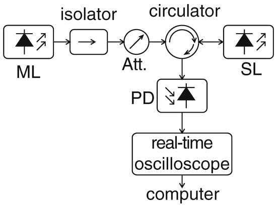
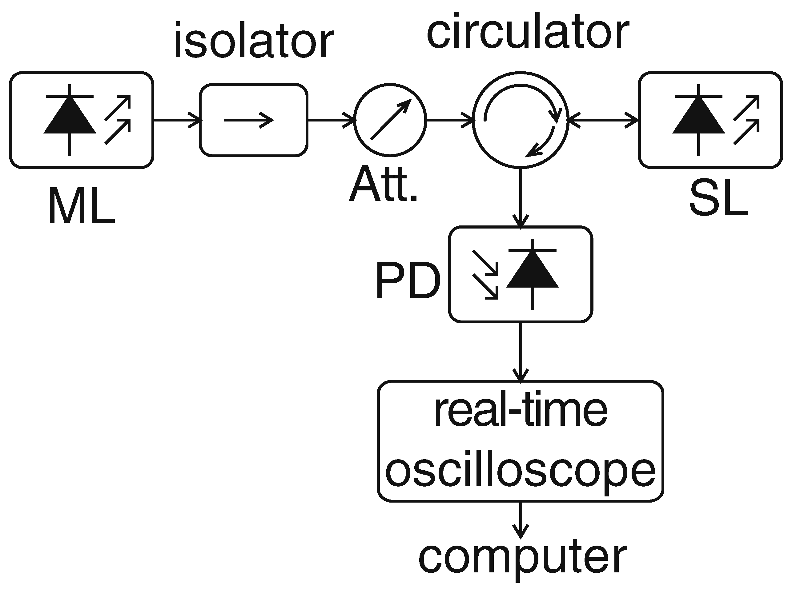
Figure 1 illustrates a representative experimental configuration for optical injection in semiconductor lasers [14]. The master laser (ML) output passes through an optical isolator and a variable attenuator before being injected into the slave laser (SL). The resulting emission from the slave laser is monitored using a high-speed photodetector (PD), enabling experimental observation of injection locking and chaotic dynamics.

Figure 1. Experimental configuration for optically injected semiconductor lasers: ML: master laser, Att.: optical attenuator, SL: slave laser, and PD: photodetector [14].

A central objective of this work is to assess the numerical reliability of Lyapunov-exponent-based chaos characterization in optically injected semiconductor lasers for different coordinate representations. Particular attention is devoted to identifying and quantifying numerical artifacts that may arise in variational calculations when the optical field amplitude approaches low values.

The main contributions of this paper are:

• A systematic numerical reliability assessment of Lyapunov-based chaos analysis in optically injected semiconductor lasers using both phasor $(A,\psi ,N)$ and quadrature $(X,Y,N)$ representations.
• A direct comparison of high-resolution Lyapunov maps computed in both coordinate systems, demonstrating that while the overall dynamical structure is preserved, the phasor formulation may introduce spurious chaotic regions due to singular terms proportional to $1/A$ and $1/A^2$ in the variational Jacobian.
• Identification and quantitative characterization of the principal numerical pitfalls affecting Lyapunov exponent estimation, including low-amplitude singularities, phase-handling inconsistencies, and sensitivity of the variational dynamics to coordinate representation.
• Demonstration that the quadrature formulation provides numerically stable and physically consistent Lyapunov spectra across the explored parameter space, establishing it as a robust framework for large-scale chaos mapping in optically injected semiconductor lasers.
• Practical implementation guidelines and a reproducible Lyapunov-based classification strategy for automated detection of chaotic regimes in extensive parameter scans.

By shifting the emphasis from the discovery of new chaotic regimes to the numerical reliability and reproducibility of chaos quantification itself, this work provides a rigorous methodological framework for Lyapunov-based analysis in optically injected semiconductor lasers and related nonlinear photonic systems.

The remainder of the paper is organized as follows. Section 2 presents the theoretical model and numerical methodology used for Lyapunov exponent computation in both phasor and quadrature formulations. Section 3 presents high-resolution Lyapunov maps and a detailed comparison between formulations. Section 4 discusses numerical reliability and practical implementation guidelines for chaos diagnostics. Finally, Section 5 summarizes the main conclusions and outlines possible extensions of this framework to other nonlinear photonic systems.

2. Method

This section presents the numerical methodology used to compute Lyapunov spectra and chaoticity maps in optically injected semiconductor lasers. We consider two equivalent representations of the optical field: (i) the phasor (polar) formulation in terms of amplitude and relative phase, $x_p\left(t\right)=(A\left(t\right),\psi \left(t\right),N\left(t\right))$, and (ii) the Cartesian quadrature formulation, $x_q\left(t\right)=(X\left(t\right),Y\left(t\right),N\left(t\right))$, where $E\left(t\right)=X\left(t\right)+iY\left(t\right)$. Although both descriptions are related by a smooth change of coordinates away from $A=0$, their variational implementations differ in numerical robustness because the phasor Jacobian contains terms proportional to $1/A$ and $1/A^2$. We therefore implement the same deterministic variational RK4-QR scheme in both coordinate systems and compare the resulting Lyapunov spectra and parameter-space maps, explicitly identifying conditions under which numerical artifacts may lead to spurious chaos diagnostics.

To rigorously characterize deterministic chaos in OILs, spontaneous emission and Langevin noise must be removed as they can obscure intrinsic nonlinear dynamics and mimic chaotic behavior [29,30]. These stochastic perturbations distort phase-space structures, compromise reproducibility, and affect key chaos indicators such as Lyapunov exponents and correlation measures [31,32]. By suppressing noise, the observed complexity can be attributed unambiguously to deterministic mechanisms governed by injection parameters and carrier-photon interactions.

2.1. Phasor Rate Equations with Known Delayed Injection

Let the injected amplitude and phase be known functions of time:

$$A_{\mathrm{inj}}(t-\tau )=\eta A_0,{\varphi }_{\mathrm{inj}}(t-\tau )={\omega }_{\mathrm{inj}}(t-\tau ),$$

(1)

where $A_0$ is the nominal amplitude of the master laser, $\eta \in (0,1]$ models attenuation in the fiber, and ${\omega }_{\mathrm{inj}}$ is the angular frequency of the injected field. To eliminate explicit time dependence in the injection terms, define the relative phase

$$\psi \left(t\right):=\varphi \left(t\right)-{\omega }_{\mathrm{inj}}t.$$

(2)

It is important to distinguish between the two phase variables. The quantity $\varphi \left(t\right)$ denotes the instantaneous optical phase of the slave laser field, whereas ${\varphi }_{\mathrm{inj}}(t-\tau )$ represents the optical phase of the injected (master) field after propagation through the fiber with delay $\tau$. The relative phase $\psi \left(t\right)=\varphi \left(t\right)-{\omega }_{\mathrm{inj}}t$ therefore measures the offset between the slave’s phase and that of the injected reference oscillating at frequency ${\omega }_{\mathrm{inj}}$. Then the trigonometric arguments simplify as

$$\varphi \left(t\right)-{\omega }_{\mathrm{inj}}(t-\tau )=\psi \left(t\right)+{\omega }_{\mathrm{inj}}\tau ,$$

(3)

which is independent of t. The normalized system is therefore

$$\left\{\begin{array}{cc}\hfill \dot{A}\left(t\right)& =\frac{1}{2}g\left(N\left(t\right)-N_{\mathrm{th}}\right)A\left(t\right)+k_{\mathrm{inj}}\eta A_{0}cos\left(\psi \left(t\right)+{\omega }_{\mathrm{inj}}\tau \right),\hfill \\ \hfill \dot{\psi }\left(t\right)& =\frac{\alpha }{2}g\left(N\left(t\right)-N_{\mathrm{th}}\right)-{\displaystyle \frac{k_{\mathrm{inj}}\eta A_0}{A\left(t\right)}}sin\left(\psi \left(t\right)+{\omega }_{\mathrm{inj}}\tau \right)+\Delta \omega ,\hfill \\ \hfill \dot{N}\left(t\right)& =J-{\gamma }_{N}N\left(t\right)-\left({\gamma }_P+g\left(N\left(t\right)-N_{\mathrm{th}}\right)\right)A{\left(t\right)}^2.\hfill \end{array}\right.$$

(4)

Here, g is the linear gain coefficient, $\alpha$ is the linewidth enhancement factor, J is the carrier injection rate, ${\gamma }_P$ is the photon decay rate, and ${\gamma }_N$ is the carrier recombination rate. The detuning frequency is defined as

$$\Delta \omega :={\omega }_{\mathrm{slave}}-{\omega }_{\mathrm{inj}},$$

(5)

so that positive detuning corresponds to a blue-shifted slave frequency. The coupling coefficient $k_{\mathrm{inj}}$ accounts for the injection strength and depends on the mirror reflectivity r, the injection efficiency $r_{\mathrm{inj}}$, and the round-trip time ${\tau }_{\mathrm{in}}$, given by

$$k_{\mathrm{inj}}={\displaystyle \frac{(1-r^2)r_{\mathrm{inj}}}{{\tau }_{\mathrm{in}}r}}.$$

(6)

In this normalized form the system is autonomous. The delay appears only as a constant phase offset ${\omega }_{\mathrm{inj}}\tau$ inside the trigonometric functions, which greatly simplifies both numerical integration and the application of the variational method for Lyapunov spectrum computation. Numerical simulations of the OIL system were performed using the parameter set of Table 1 based on representative semiconductor laser characteristics reported in the literature [14,33] and covering the injection-strength and detuning ranges explored in the chaos maps.

Table 1. Simulation parameters of the OIL system, including control parameter ranges, based on [14,33].

Laser Parameter	Symbol	Value/Range	Unit
Nominal wavelength	$\lambda$	1550	nm
Linear gain coefficient	g	$5.666\times {10}^3$	1/s
Transparency carrier number	$N_{\mathrm{tr}}$	$1.626\times {10}^8$	-
Carrier number threshold	$N_{\mathrm{th}}$	$2.214\times {10}^8$	-
Linewidth enhancement factor	$\alpha$	3	-
Electron flux	J	$10\times J_{\mathrm{th}}$	1/s
Electron flux threshold	$J_{\mathrm{th}}$	$6.2414\times {10}^{16}$	1/s
Carrier recombination rate	${\gamma }_{\mathrm{N}}$	${10}^9$	1/s
Photon decay rate	${\gamma }_{\mathrm{P}}$	$3.333\times {10}^{11}$	1/s
Mirror reflectivity	r	0.548	-
Coupling coefficient	$k_{\mathrm{inj}}$	$1.824\times {10}^{11}$	1/s
Round-trip time	${\tau }_{\mathrm{in}}$	$7\times {10}^{-12}$	s
Simulation time step	$\Delta t$	1	ps
Frequency detuning (control parameter)	$\Delta {\omega }_{\mathrm{inj}}$	0 to 6	GHz
Injection strength (control parameter)	$A_{\mathrm{inj}}$	0 to $-40$	dB
Fiber delay	$\tau$	3.95, 5, 6.58	ns

2.2. Jacobian Matrix of the Phasor Variational Analysis

The full Lyapunov spectrum of the normalized OIL system is obtained using the variational method, which integrates the nonlinear trajectory together with the tangent-space dynamics [34,35]. The state vector is

$$x\left(t\right)=\left[\begin{array}{c}A\left(t\right)\\ \psi \left(t\right)\\ N\left(t\right)\end{array}\right],$$

(7)

and the governing equations are given in Equations (1)–(3). Let $\theta :=\psi +{\omega }_{\mathrm{inj}}\tau$ (a constant phase offset inside the trigonometric terms). The Jacobian with respect to x is

$$J\left(x\right)=\left[\begin{array}{ccc}{\displaystyle \frac{1}{2}}g(N-N_{\mathrm{th}})& -k_{\mathrm{inj}}\eta A_{0}sin\theta & {\displaystyle \frac{1}{2}}gA\\ {\displaystyle \frac{k_{\mathrm{inj}}\eta A_0}{A^2}sin\theta }& {\displaystyle -\frac{k_{\mathrm{inj}}\eta A_0}{A}cos\theta }& {\displaystyle \frac{\alpha }{2}g}\\ -2A\left({\gamma }_P+g(N-N_{\mathrm{th}})\right)& 0& -{\gamma }_N-g{A}^2\end{array}\right].$$

(8)

Note that $\Delta \omega$ is constant, so its derivatives vanish. The Jacobian is evaluated at every integration step and governs the tangent-space evolution $\dot{Q}=J\left(x\right)Q.$ Its explicit analytical form enables direct and accurate RK4 integration of the variational dynamics together with periodic QR orthonormalization, eliminating the need for numerical differentiation of partial derivatives.

2.3. Fourth-Order RK Integration of the Phasor Dynamics

Both the base system $x\left(t\right)$ and the variational dynamics $Q\left(t\right)$ are integrated using the classical fourth-order Runge-Kutta (RK4) scheme. This approach ensures numerical consistency and stability across both trajectories.

2.3.1. Phasor System RK4 Integration

Let $x_n$ denote the system state at time $t_n$ and $dt$ the time step. The standard RK4 update is

$$\left\{\begin{array}{cc}\hfill k_1^x& =f(t_n,x_n),\hfill \\ \hfill k_2^x& =f\left(t_n+\frac{dt}{2},x_n+\frac{dt}{2}{k}_1^x\right),\hfill \\ \hfill k_3^x& =f\left(t_n+\frac{dt}{2},x_n+\frac{dt}{2}{k}_2^x\right),\hfill \\ \hfill k_4^x& =f\left(t_n+dt,x_n+dt·k_3^x\right).\hfill \end{array}\right.$$

(9)

2.3.2. Phasor Tangent-Space RK4 Integration

Let $Q_n$ be the tangent-space matrix at step n. Using the Jacobian J evaluated at the RK4 substeps of $x_n$, we integrate the variational equation:

$$\left\{\begin{array}{cc}\hfill J_1& =J(t_n,x_n),k_1^Q=J_1{Q}_n\hfill \\ \hfill J_2& =J\left(t_n+\frac{dt}{2},x_n+\frac{dt}{2}{k}_1^x\right),k_2^Q=J_2\left(Q_n+\frac{dt}{2}{k}_1^Q\right)\hfill \\ \hfill J_3& =J\left(t_n+\frac{dt}{2},x_n+\frac{dt}{2}{k}_2^x\right),k_3^Q=J_3\left(Q_n+\frac{dt}{2}{k}_2^Q\right)\hfill \\ \hfill J_4& =J\left(t_n+dt,x_n+dt·k_3^x\right),k_4^Q=J_4\left(Q_n+dt·k_3^Q\right)\hfill \end{array}\right.$$

(10)

$$x_{n+1}=x_n+{\displaystyle \frac{dt}{6}}\left(k_1^x+2k_2^x+2k_3^x+k_4^x\right),$$

(11)

$$Q_{n+1}=Q_n+{\displaystyle \frac{dt}{6}}\left(k_1^Q+2k_2^Q+2k_3^Q+k_4^Q\right).$$

(12)

To guarantee numerical consistency in the variational Lyapunov analysis, particular care must be taken when evaluating the Jacobian of the phasor-based OIL model. In the master-slave configuration, several terms in the phase dynamics and in the linearized system contain divisions by the field amplitude, specifically factors proportional to $1/A\left(t\right)$ and $1/A{\left(t\right)}^2$. When the amplitude approaches zero, these terms become singular and the Jacobian may become ill-conditioned. Such near-zero amplitude events can arise during transient dynamics even when the laser remains physically active. In this situation the tangent-space evolution may exhibit artificially large stretching factors, which can lead to spurious positive Lyapunov exponents unrelated to the underlying deterministic dynamics. A common numerical remedy consists in introducing an effective amplitude floor,

$$A_{\mathrm{eff}}\left(t\right)=sign\left(A\left(t\right)\right)max\left(\left|A\left(t\right)\right|,A_{\mathrm{floor}}\right),$$

(13)

and replacing $A\left(t\right)$ by $A_{\mathrm{eff}}\left(t\right)$ in the terms involving $1/A$ and $1/A^2$. While this regularization prevents numerical blow-up of the Jacobian, it also alters the original dynamical system and may therefore modify the computed Lyapunov spectrum.

For this reason, the phasor equations are left unmodified in the present work. Instead, parameter points for which the trajectory approaches the zero-amplitude manifold are treated as numerically unreliable in the variational computation. This choice allows a direct comparison between the phasor formulation and the quadrature representation, where the dynamical equations do not contain divisions by the field amplitude. As shown in the results section, the quadrature-based computation yields consistent chaos maps, whereas the phasor formulation becomes unreliable whenever the trajectory approaches $A\left(t\right)\approx 0$.

A fixed integration step of 1 ps was used for the fourth-order Runge-Kutta scheme in both the trajectory and variational equations. This step size provides sufficient temporal resolution to accurately capture the fastest intrinsic oscillations of the system, including relaxation-oscillation dynamics in the GHz range and higher-frequency modulations observed in strongly chaotic regimes. Additional convergence tests with smaller time steps were performed over representative regions of the parameter space and showed no observable changes in the Lyapunov spectra or in the global structure of the chaos maps within numerical precision. The selected step therefore ensures accurate and stable integration while maintaining computational feasibility for the high-resolution parameter sweeps presented in this work.

2.4. Real-Quadrature Formulation of the OIL Rate Equations

We represent the slave electric field in real quadratures,

$$E\left(t\right)=X\left(t\right)+{iY\left(t\right),\left|E\left(t\right)\right|}^2=X{\left(t\right)}^2+Y{\left(t\right)}^2,$$

(14)

where $X\left(t\right)$ and $Y\left(t\right)$ are the in-phase and quadrature components, respectively. The injected (master) field is assumed to have known amplitude and phase after propagation through a fiber of delay $\tau$:

$$A_{\mathrm{inj}}(t-\tau )=\eta A_0,{\varphi }_{\mathrm{inj}}(t-\tau )={\omega }_{\mathrm{inj}}(t-\tau ),$$

(15)

where $A_0$ is the nominal master amplitude, $\eta \in (0,1]$ accounts for attenuation in the fiber, and ${\omega }_{\mathrm{inj}}$ is the angular frequency of the injected field. In a feedforward master-delay-slave configuration (no optical feedback), the delay enters the slave dynamics only through the phase of the injected field, i.e., as a constant phase shift $-{\omega }_{\mathrm{inj}}\tau$ multiplying the injected complex amplitude. Accordingly, the injected term can be written as the constant complex phasor

$$E_{\mathrm{inj}}(t-\tau )=\eta A_0{e}^{i{\varphi }_{\mathrm{inj}}(t-\tau )}=\eta A_0{e}^{i{\omega }_{\mathrm{inj}}t}{e}^{-i{\omega }_{\mathrm{inj}}\tau }.$$

(16)

Working in the rotating frame at ${\omega }_{\mathrm{inj}}$ eliminates the explicit time dependence and yields a constant injection phasor

$${\tilde{E}}_{\mathrm{inj}}=\eta A_0{e}^{-i{\omega }_{\mathrm{inj}}\tau }.$$

(17)

Let $\Delta \omega :={\omega }_{\mathrm{slave}}-{\omega }_{\mathrm{inj}}$ denote the detuning frequency. Using the standard complex field equation for an optically injected semiconductor laser in amplitude form, the noise-free normalized dynamics in the rotating frame can be expressed as

$$\dot{E}\left(t\right)={\displaystyle \frac{1}{2}}(1+i\alpha )g\left(N\left(t\right)-N_{\mathrm{th}}\right)E\left(t\right)+i\Delta \omega E\left(t\right)+k_{\mathrm{inj}}{\tilde{E}}_{\mathrm{inj}},$$

(18)

together with the carrier equation

$$\dot{N}\left(t\right)=J-{\gamma }_{N}N\left(t\right)-\left({\gamma }_P+g\left(N\left(t\right)-N_{\mathrm{th}}\right)\right){\left|E\left(t\right)\right|}^2.$$

(19)

Separating real and imaginary parts yields an equivalent autonomous three-dimensional real system:

$$\left\{\begin{array}{cc}\hfill \dot{X}\left(t\right)& ={\displaystyle \frac{1}{2}}g\left(N\left(t\right)-N_{\mathrm{th}}\right)X\left(t\right)-\left(\Delta \omega +{\displaystyle \frac{\alpha }{2}}g\left(N\left(t\right)-N_{\mathrm{th}}\right)\right)Y\left(t\right)+k_{\mathrm{inj}}\eta A_{0}cos\left({\omega }_{\mathrm{inj}}\tau \right),\hfill \\ \hfill \dot{Y}\left(t\right)& ={\displaystyle \frac{1}{2}}g\left(N\left(t\right)-N_{\mathrm{th}}\right)Y\left(t\right)+\left(\Delta \omega +{\displaystyle \frac{\alpha }{2}}g\left(N\left(t\right)-N_{\mathrm{th}}\right)\right)X\left(t\right)-k_{\mathrm{inj}}\eta A_{0}sin\left({\omega }_{\mathrm{inj}}\tau \right),\hfill \\ \hfill \dot{N}\left(t\right)& =J-{\gamma }_{N}N\left(t\right)-\left({\gamma }_P+g\left(N\left(t\right)-N_{\mathrm{th}}\right)\right)\left(X{\left(t\right)}^2+Y{\left(t\right)}^2\right).\hfill \end{array}\right.$$

(20)

Here, g is the linear gain coefficient, $\alpha$ is the linewidth enhancement factor, J is the carrier injection rate, ${\gamma }_P$ is the photon decay rate, and ${\gamma }_N$ is the carrier recombination rate. The coupling coefficient $k_{\mathrm{inj}}$ accounts for the injection strength and depends on the mirror reflectivity r, the injection efficiency $r_{\mathrm{inj}}$, and the round-trip time ${\tau }_{\mathrm{in}}$:

$$k_{\mathrm{inj}}={\displaystyle \frac{(1-r^2)r_{\mathrm{inj}}}{{\tau }_{\mathrm{in}}r}}.$$

(21)

In this quadrature formulation the dynamics are autonomous and the delay appears only through the constant phase shift ${\omega }_{\mathrm{inj}}\tau$ in the injected phasor. Importantly, the system (20) contains no divisions by the field amplitude, avoiding the coordinate singularity present in polar $(A,\psi )$ representations when $A\left(t\right)\to 0$.

2.5. Jacobian Matrix of the Quadrature OIL System

We compute the full Lyapunov spectrum of the normalized OIL system by the variational method, integrating both the nonlinear trajectory and the tangent-space dynamics [34,35]. The state vector is

$$x\left(t\right)=\left[\begin{array}{c}X\left(t\right)\\ Y\left(t\right)\\ N\left(t\right)\end{array}\right],$$

(22)

and the governing equations are given by (20). Define

$$G:=g\left(N-N_{\mathrm{th}}\right),\Omega :=\Delta \omega +{\displaystyle \frac{\alpha }{2}}G.$$

(23)

Then the Jacobian with respect to x is

$$J\left(x\right)=\left[\begin{array}{ccc}{\displaystyle \frac{1}{2}}G& -\Omega & {\displaystyle \frac{g}{2}}X-{\displaystyle \frac{\alpha g}{2}}Y\\ \Omega & {\displaystyle \frac{1}{2}}G& {\displaystyle \frac{\alpha g}{2}}X+{\displaystyle \frac{g}{2}}Y\\ -2X\left({\gamma }_P+G\right)& -2Y\left({\gamma }_P+G\right)& -{\gamma }_N-g(X^2+Y^2)\end{array}\right].$$

(24)

Note that the constant injection terms do not contribute to the Jacobian. This Jacobian is evaluated at each integration step and is used to integrate the tangent dynamics $\dot{Q}=J\left(x\right)Q$.

2.6. Fourth-Order Runge–Kutta Integration of the Quadrature Dynamics

Both the base system $x\left(t\right)$ and the variational dynamics $Q\left(t\right)$ are integrated using the classical fourth-order Runge-Kutta (RK4) scheme. Let

$$x\left(t\right)=\left[\begin{array}{c}X\left(t\right)\\ Y\left(t\right)\\ N\left(t\right)\end{array}\right],$$

where $X\left(t\right)$ and $Y\left(t\right)$ are the real and imaginary quadratures of the electric field and $N\left(t\right)$ is the carrier density. The system dynamics are written compactly as

$$\dot{x}\left(t\right)=f\left(t,x\left(t\right)\right),$$

with f given by the right-hand side of (20). The tangent-space dynamics satisfy

$$\dot{Q}\left(t\right)=J\left(t,x\left(t\right)\right)Q\left(t\right),$$

where J is the Jacobian matrix in (24).

Let $x_n\approx x\left(t_n\right)$ and $Q_n\approx Q\left(t_n\right)$, with time step $dt=t_{n+1}-t_n$. The RK4 update for the nonlinear system is

$$\left\{\begin{array}{cc}\hfill k_1^x& =f\left(t_n,x_n\right),\hfill \\ \hfill k_2^x& =f\left(t_n+\frac{dt}{2},x_n+\frac{dt}{2}{k}_1^x\right),\hfill \\ \hfill k_3^x& =f\left(t_n+\frac{dt}{2},x_n+\frac{dt}{2}{k}_2^x\right),\hfill \\ \hfill k_4^x& =f\left(t_n+dt,x_n+dt{k}_3^x\right),\hfill \end{array}\right.$$

(25)

$$x_{n+1}=x_n+{\displaystyle \frac{dt}{6}}\left(k_1^x+2k_2^x+2k_3^x+k_4^x\right).$$

(26)

In parallel, the RK4 integration of the tangent-space dynamics is performed using the Jacobian evaluated at the same intermediate states:

$$\left\{\begin{array}{cccc}\hfill J_1& =J\left(t_n,x_n\right),\hfill & \hfill k_1^Q& =J_1{Q}_n,\hfill \\ \hfill J_2& =J\left(t_n+\frac{dt}{2},x_n+\frac{dt}{2}{k}_1^x\right),\hfill & \hfill k_2^Q& =J_2\left(Q_n+\frac{dt}{2}{k}_1^Q\right),\hfill \\ \hfill J_3& =J\left(t_n+\frac{dt}{2},x_n+\frac{dt}{2}{k}_2^x\right),\hfill & \hfill k_3^Q& =J_3\left(Q_n+\frac{dt}{2}{k}_2^Q\right),\hfill \\ \hfill J_4& =J\left(t_n+dt,x_n+dt{k}_3^x\right),\hfill & \hfill k_4^Q& =J_4\left(Q_n+dt{k}_3^Q\right).\hfill \end{array}\right.$$

(27)

The tangent matrix is then updated as

$$Q_{n+1}=Q_n+{\displaystyle \frac{dt}{6}}\left(k_1^Q+2k_2^Q+2k_3^Q+k_4^Q\right).$$

(28)

Because the quadrature formulation (20) contains no divisions by the field amplitude, the nonlinear system and its Jacobian are free of singular terms proportional to $1/A$ or $1/A^2$. Consequently, no amplitude-floor regularization is required in either the base dynamics or the variational equations. This guarantees that the tangent-space evolution remains well conditioned and that all positive Lyapunov exponents arise from genuine deterministic instability rather than numerical artifacts.

The computation of the Lyapunov spectrum is carried out independently for both coordinate representations described above, namely, the phasor formulation $(A,\psi ,N)$ and the Cartesian quadrature formulation $(X,Y,N)$. In each case, the nonlinear system and its corresponding Jacobian are integrated simultaneously using the fourth-order Runge-Kutta scheme and identical numerical parameters.

The subsequent extraction of Lyapunov exponents follows an identical procedure for both models. In particular, the tangent-space dynamics are periodically orthonormalized using a QR decomposition, and the Lyapunov exponents are obtained from the logarithmic growth rates of the diagonal elements of the resulting upper triangular matrices. This unified post-processing ensures that any differences observed between the two formulations arise solely from their coordinate representations and numerical properties, rather than from inconsistencies in the Lyapunov computation itself.

2.7. QR Decomposition and Lyapunov Exponents

To prevent numerical divergence and maintain orthonormality of tangent vectors, the variational equations are integrated alongside the nonlinear system and orthonormalized at each time step using a QR decomposition,

$$Q_{n+1}=Q_{n+1}^{\left(Q\right)}{R}_n,\left(Q_{n+1}^{\left(Q\right)},R_n\right)=\mathrm{qr}\left(Q_{n+1}\right),$$

(29)

where $Q_{n+1}^{\left(Q\right)}$ has orthonormal columns and $R_n$ is an upper triangular matrix whose diagonal elements capture the local stretching rates of nearby trajectories.

The Lyapunov exponents are obtained from the long-time averages of the logarithmic growth rates of the diagonal elements of $R_n$,

$${\lambda }_i=\underset{T\to \infty }{lim}{\displaystyle \frac{1}{T}}\sum _{n=1}^{N\left(T\right)}log\left|R_{ii}\left(t_n\right)\right|,i=1,\dots ,m,$$

(30)

where $m=3$ for the state vector $x\left(t\right)={[X\left(t\right),Y\left(t\right),N\left(t\right)]}^{\top }$ and $T\approx N\Delta t$ is the total integration time in the case of quadrature formulation.

In practice, the instantaneous values of $log|R_{11}\left(t\right)|$ often exhibit strong temporal oscillations and may not converge pointwise. Direct averaging over a single arbitrary window can therefore introduce bias in the estimated Lyapunov spectrum. To reduce this sensitivity, we adopt a window-based averaging strategy designed to assess the temporal persistence of exponential divergence.

Specifically, we identify two sets of time indices where the dominant stretching rate satisfies $|log{R}_{11}\left(t\right)|<ϵ$, with a small threshold $ϵ$. One set is selected from an early post-transient interval (e.g., $t\in [20,30]$ ns), while the second is taken from the final portion of the simulation (e.g., $t\in [190,200]$ ns). For each admissible pair of start and end indices $(n_s,n_e)$ with $t_{n_e}>t_{n_s}$, the Lyapunov spectrum was computed as

$${\lambda }_i^{\left(k\right)}={\displaystyle \frac{1}{t_{n_e}-t_{n_s}}}\sum _{n=n_s}^{n_e-1}log\left|R_{ii}\left(t_n\right)\right|,i=1,2,3,$$

(31)

where k indexes the $(n_s,n_e)$ window combination. This procedure yields an ensemble of local estimates ${\left\{{\lambda }_i^{\left(k\right)}\right\}}_{k=1}^{N_c}$ from which the mean Lyapunov spectrum ${\overline{\lambda }}_i$ is obtained.

Rather than relying solely on the mean value of the dominant exponent, we quantify the robustness of chaos by evaluating the fraction of window combinations for which the largest Lyapunov exponent is positive:

$$p_{\mathrm{pos}}={\displaystyle \frac{1}{N_c}}\sum _{k=1}^{N_c}\mathbb{I}\left({\lambda }_1^{\left(k\right)}>0\right),$$

(32)

where $\mathbb{I}(·)$ is the indicator function. The quantity $p_{\mathrm{pos}}$ measures the temporal persistence of exponential divergence in the dynamics.

A dynamical regime is classified as chaotic only if the mean largest Lyapunov exponent satisfies ${\overline{\lambda }}_1>0$ and if $p_{\mathrm{pos}}$ exceeds a prescribed threshold. In this work, three robustness levels are defined: $p_{\mathrm{pos}}\ge 0.50$ indicates intermittent chaos, $p_{\mathrm{pos}}\ge 0.75$ corresponds to robust chaos, and $p_{\mathrm{pos}}\ge 0.90$ defines strongly robust chaos. This percentage-based criterion ensures that chaos is not inferred from isolated temporal windows or numerical fluctuations but from a persistent exponential separation of nearby trajectories over a significant portion of the simulated dynamics.

2.8. Relaxation Oscillation Frequency

To verify the internal consistency of the rate-equation normalization and the associated time scales, we compute the small-signal relaxation oscillation frequency of the solitary slave laser (no optical injection) directly from the eigenvalues of the Jacobian evaluated at the free-running steady state.

Linearization of the quadrature system around the equilibrium $(X^{*},Y^{*},N^{*})$ yields one neutral eigenvalue associated with phase invariance and one complex-conjugate pair

$${\mu }_{2,3}=-\sigma \pm i{\Omega }_R,$$

where ${\mu }_{2,3}$ are the complex-conjugate eigenvalues of the Jacobian $J\left(x^{*}\right)$ at the steady state $x^{*}={(X^{*},Y^{*},N^{*})}^{\top }$, $\sigma >0$ is the damping rate (real part), and ${\Omega }_R$ is the angular relaxation-oscillation frequency (rad/s), defined as ${\Omega }_R=Im\left({\mu }_{2,3}\right)$. The relaxation oscillation frequency in hertz is therefore

$$f_R={\displaystyle \frac{{\Omega }_R}{2\pi }}.$$

Using the parameter set of Table 1, the eigenvalue analysis yields

$${\mu }_{2,3}=-3.92\times {10}^9\pm i4.76\times {10}^{10},$$

corresponding to a relaxation oscillation frequency

$$f_R\approx 7.58\mathrm{GHz}.$$

Because this value is obtained directly from the Jacobian of the governing rate equations, it provides a self-consistent reference frequency for the characteristic time scales of the system and for the Lyapunov-based dynamical analysis presented in the following sections.

2.9. Advantages of the Variational Method

The variational method provides a fully deterministic and high-resolution estimation of the Lyapunov spectrum by directly integrating the governing equations together with their Jacobian. Because the procedure operates on the exact dynamical model rather than on reconstructed trajectories, it is unaffected by measurement noise, finite data length, or embedding ambiguities that typically affect time-series-based estimators.

Historically, chaos in optically injected semiconductor lasers has often been identified using time-series indicators such as Rosenstein or Wolf Lyapunov estimators. While appropriate for experimental data, these methods depend on embedding and filtering choices and may introduce variability in purely numerical studies. In deterministic simulations where the full state equations and Jacobian are available, such approximations are unnecessary. Consistency between the exact variational Lyapunov computation and Rosenstein [36]-type estimators was verified in our earlier work [28], where both yielded closely matching largest Lyapunov exponents; therefore, only the variational results are reported here.

In contrast, the variational approach yields the complete Lyapunov spectrum through the evolution of tangent vectors governed by the exact Jacobian of the system. This ensures coordinate-invariant and reproducible results, enabling precise identification of stability transitions between injection locking, quasi-periodicity, and deterministic chaos. Moreover, the method is particularly well suited for large parameter scans as it provides consistent estimates across the entire parameter space without requiring heuristic tuning of reconstruction parameters.

For optically injected laser models, where small numerical inconsistencies can lead to spurious positive exponents, the variational formulation offers a rigorous and transparent framework for chaos detection. Its deterministic nature allows direct comparison between alternative coordinate representations, such as phasor and quadrature formulations, ensuring that any observed differences in Lyapunov spectra originate from model formulation or numerical conditioning rather than from limitations of the chaos estimator itself.

2.10. Kaplan-Yorke Dimension

The Kaplan-Yorke (KY) dimension, also referred to as the Lyapunov dimension, provides an estimate of the fractal dimension of an attractor based on the ordered Lyapunov spectrum [37]. Given the exponents ${\lambda }_1\ge {\lambda }_2\ge \cdots \ge {\lambda }_m$, the KY dimension is defined as

$$D_{KY}=j+{\displaystyle \frac{{\sum }_{i=1}^j{\lambda }_i}{|{\lambda }_{j+1}|}},$$

(33)

where j is the largest integer such that ${\sum }_{i=1}^j{\lambda }_i\ge 0$.

For the present three-dimensional master-delay-slave configuration, the Kaplan-Yorke dimension is expected to remain below 2 since the system possesses at most one effective expanding direction in phase space and does not exhibit hyperchaotic behavior. In this context, values of $D_{KY}$ close to 2 correspond to strongly developed chaos with a fully unfolded strange attractor, whereas values in the interval $1<D_{KY}<2$ indicate weaker low-dimensional chaos. Periodic oscillations typically yield $D_{KY}\approx 1$, while stable fixed points correspond to $D_{KY}\approx 0$.

Values approaching 3 would require the activation of an additional independent expanding direction and are therefore associated with higher-dimensional or feedback-based laser configurations rather than the feedforward master-delay-slave system considered here. Consequently, in the present analysis the observed $D_{KY}$ values close to 2 represent the maximum attainable chaotic dimensionality for this class of optically injected laser systems.

Mapping $D_{KY}$ over injection strength and frequency detuning therefore provides a compact scalar measure of the effective number of active dynamical degrees of freedom in each regime and serves as a complementary diagnostic to the individual Lyapunov exponents. In this work, the Kaplan-Yorke dimension is used to distinguish weak chaos, strongly developed chaos, and low-dimensional regular dynamics within the same parameter space.

2.11. Dissipativity and Phase-Space Volume Contraction

The sum of the Lyapunov exponents quantifies the average rate of phase-space volume contraction and provides a global measure of dissipativity:

$$\sum _{i=1}^m{\lambda }_i=⟨\nabla ·f\left(x\right)⟩=⟨\mathrm{Tr}\left(J\left(x\right)\right)⟩,$$

(34)

where f denotes the vector field and J its Jacobian. For a three-dimensional system ($m=3$), a negative sum indicates a dissipative flow in which phase-space volumes contract on average, confining trajectories to lower-dimensional invariant sets such as fixed points, limit cycles, or strange attractors.

Strongly negative values of ${\lambda }_1+{\lambda }_2+{\lambda }_3$ correspond to rapid volume contraction and are typically associated with stable or weakly oscillatory regimes. Conversely, values closer to zero indicate weaker dissipation, allowing stretching and folding mechanisms to persist and enabling the development of complex or chaotic dynamics. In this study, the total Lyapunov sum was computed throughout the parameter space to generate dissipativity maps that complement the Lyapunov and Kaplan-Yorke analyses, highlighting regions where chaos is sustained under moderate dissipation conditions and in regions where it is suppressed by strong phase-space contraction.

3. Results

We computed the largest Lyapunov exponent and the complete Lyapunov spectrum using the exact variational method, which integrates the nonlinear rate equations together with their Jacobian dynamics and applies QR orthonormalization at each time step. All results presented below correspond to systematic sweeps of the relevant parameter space and include outcomes obtained from both the phasor and Cartesian quadrature formulations.

Each chaos map was constructed from a two-dimensional sweep over injection strength and frequency detuning, where every pixel represents the evaluation of a chaos indicator at a specific parameter pair. Smooth color gradients indicate gradual dynamical variation, whereas sharp contrasts mark transitions between periodic, quasi-periodic, and chaotic regimes. The apparent pixelation of the maps is therefore a direct consequence of the parameter grid resolution and the intrinsic nonlinear structure of the system rather than a graphical artifact.

All simulations were performed in MATLAB 2025 using double-precision arithmetic and custom deterministic RK4 variational solvers for Lyapunov spectrum computation. The parameter sweeps required approximately 72,000 independent simulations, each involving simultaneous integration of the nonlinear rate equations and their associated variational Jacobian system. Computations were executed on workstation-class desktop computers equipped with multi-core x86-64 processors (AMD Ryzen-class CPUs) and 32–64 GB of RAM in a Linux/Windows environment. Parallel execution was implemented using MATLAB’s parfor functionality to distribute independent parameter points across available CPU cores. All simulations employed CPU-based numerical integration with fixed-step RK4 updates and deterministic QR orthonormalization, ensuring full reproducibility across equivalent hardware platforms.

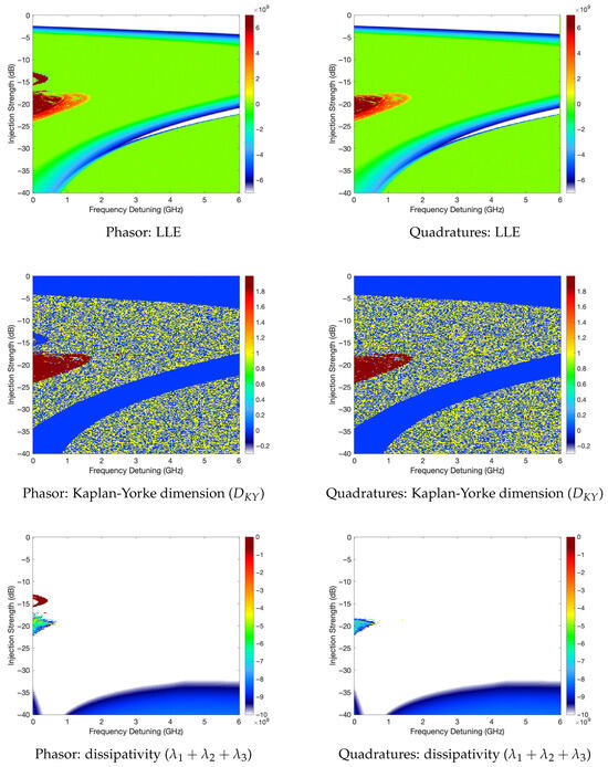
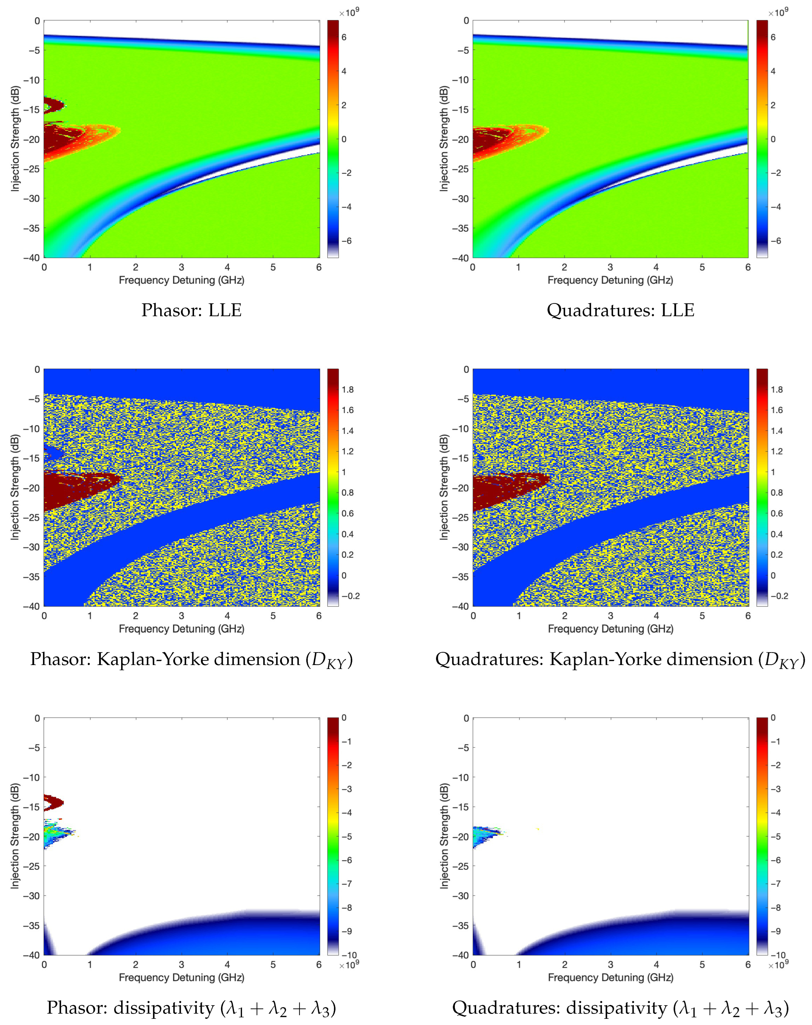
The analyzed OIL model is a three-dimensional dynamical system composed of the optical field (expressed either in phasor or Cartesian quadrature form) and the carrier density $N\left(t\right)$. The chaos maps were constructed by sweeping the injection strength $A_{\mathrm{inj}}$ (dB) and frequency detuning $\Delta {\omega }_{\mathrm{inj}}$ (GHz). In Figure 2, the horizontal axis represents detuning, the vertical axis represents injection strength, and the color scale encodes the computed chaos indicators (largest Lyapunov exponent, Kaplan-Yorke dimension, and dissipativity). The maps use a grid of 180 detuning points (≈33 MHz resolution) and 400 injection points (0.1 dB resolution), totaling 72,000 simulations, with each pixel corresponding to a complete numerical integration at a specific $(\Delta {\omega }_{\mathrm{inj}},A_{\mathrm{inj}})$ pair.

Figure 2. Side-by-side comparison of Lyapunov-based dynamical maps for the optically injected laser with fiber delay $\tau =5$ ns and robustness threshold $p_{\mathrm{pos}}\ge 0.90$. Left column: phasor formulation. Right column: Cartesian quadrature formulation. The horizontal axis denotes frequency detuning $\Delta {\omega }_{\mathrm{inj}}$ (GHz), and the vertical axis denotes injection strength (dB). Top row: largest Lyapunov exponent (LLE) maps. Positive values indicate chaotic dynamics, values near zero correspond to quasi-periodic behavior, and negative values represent periodic or stable regimes. Middle row: Kaplan-Yorke dimension maps ($D_{KY}$), encoding the effective fractal dimension of the attractor and the number of active dynamical degrees of freedom. Bottom row: dissipativity maps computed from the sum of Lyapunov exponents, indicating the phase-space volume contraction rate. The close agreement between both columns confirms that the Lyapunov spectrum and derived measures are invariant with coordinate transformation when the variational equations are implemented consistently. Local discrepancies observed in the phasor formulation near low-amplitude regions are attributable to numerical sensitivity associated with $1/A$ and $1/A^2$ terms.

Figure 2 presents a side-by-side comparison of the dynamical maps obtained using the phasor formulation (left column) and the quadrature formulation (right column) for a representative delay of $\tau =5$ ns and robustness threshold $p_{\mathrm{pos}}\ge 0.90$. The largest Lyapunov exponent maps reveal a structured organization of chaotic and non-chaotic domains, including well-defined tongues and curved boundaries that follow the underlying injection-locking and resonance conditions of the master-slave system. Warm colors correspond to positive Lyapunov exponents and deterministic chaos, green regions indicate near-zero exponents associated with quasi-periodic dynamics, and cold colors denote periodic or stable operation.

The close agreement between the two columns confirms that the global organization of chaotic and periodic regimes is preserved with coordinate transformation when the governing equations and their Jacobians are implemented consistently. At the same time, localized discrepancies appear in specific regions of the phasor maps, particularly near low-amplitude states where the presence of $1/A$ and $1/A^2$ terms increases numerical sensitivity. The quadrature formulation, which avoids divisions by the field amplitude, produces smoother and more spatially consistent maps while preserving the same global bifurcation structure.

The Kaplan-Yorke dimension maps quantify the effective fractal dimension of the attractor and therefore the dynamical complexity of the laser output. High values correspond to higher-dimensional chaotic attractors with multiple active unstable directions, whereas low values indicate periodic or weakly unstable dynamics. The similarity between the phasor and quadrature maps confirms that the fractal dimension of the attractor and its spatial distribution in parameter space are intrinsic properties of the underlying dynamical system rather than artifacts of the coordinate representation.

The dissipativity maps, obtained from the sum ${\lambda }_1+{\lambda }_2+{\lambda }_3$, provide a global measure of phase-space volume contraction. Strongly negative values correspond to highly dissipative regimes dominated by injection locking and rapid stabilization, while values closer to zero indicate weaker contraction and allow sustained stretching-folding dynamics that support chaos. These maps complement the Lyapunov and Kaplan-Yorke results by identifying parameter regions where chaotic motion is supported by a near balance between expansion and contraction.

Taken together, the three sets of maps demonstrate that the dominant dynamical organization of the optically injected semiconductor laser is governed primarily by injection strength and frequency detuning. The quadrature formulation confirms the physical robustness of the observed chaotic structures and reveals that discrepancies previously observed in certain phasor-based maps originate from numerical sensitivity rather than from genuine dynamical differences between formulations.

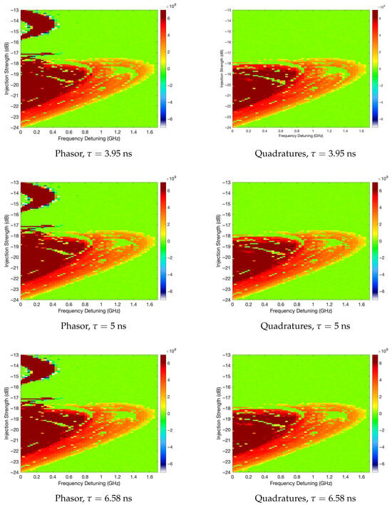
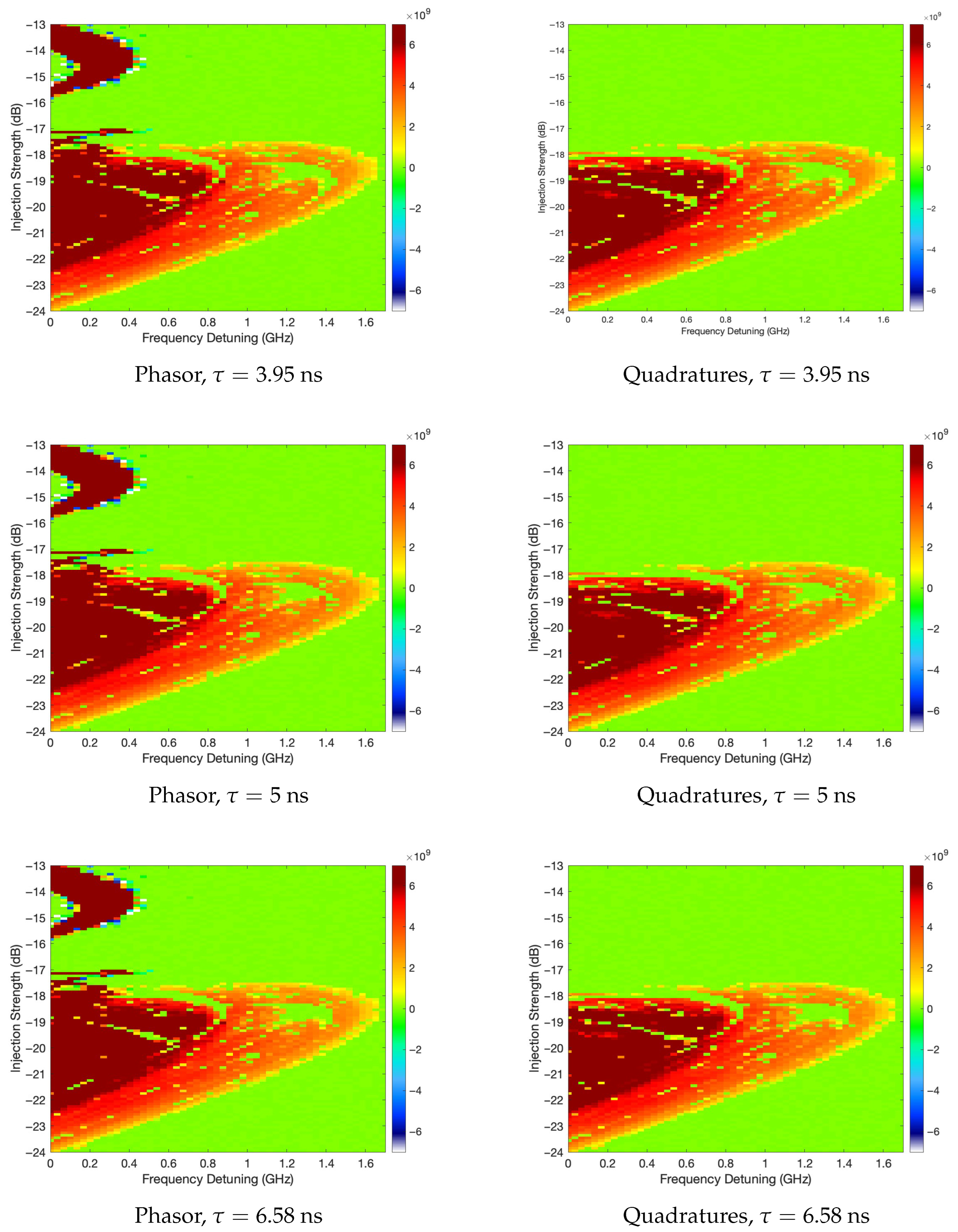
Figure 3 present a close-up comparison of the chaotic regions of the largest Lyapunov exponent (LLE) maps obtained using both the phasor and quadrature formulations for three propagation delays: $\tau =3.95$ ns, $\tau =5$ ns, and $\tau =6.58$ ns. At a global scale, the overall structure of the chaotic domains remains remarkably similar across all delay values and across both mathematical formulations, indicating that the dominant dynamical organization of the master-slave optically injected laser is largely preserved within this range of $\tau$. The close agreement between the phasor and quadrature representations confirms that the global Lyapunov structure is invariant under smooth coordinate transformation conditions when the governing equations and their Jacobians are implemented consistently.

Figure 3. Side-by-side comparison of largest Lyapunov exponent (LLE) maps obtained using the phasor formulation (left column) and the Cartesian quadrature formulation (right column) for three fiber delays: $\tau =3.95$ ns, 5 ns, and $6.58$ ns. The global structure of the chaotic regions is preserved across both formulations, consistent with invariance of Lyapunov spectra under smooth coordinate transformation conditions when the variational equations are implemented consistently. Minor localized discrepancies highlight the numerical sensitivity of the phasor formulation near low-amplitude states.

When examined at high resolution, however, subtle localized variations become visible. Small clusters of pixels shift color and the boundaries of chaotic regions exhibit slight displacements as $\tau$ varies. These modifications appear in both formulations but are more pronounced in the phasor representation near low-amplitude states, where the presence of $1/A$ and $1/A^2$ terms introduces increased numerical sensitivity. The quadrature formulation, which avoids divisions by the field amplitude, produces smoother and more spatially consistent maps while preserving the same global organization of periodic, quasi-periodic, and chaotic regimes. These observations confirm that the differences between the two approaches are primarily numerical rather than physical.

The limited influence of the propagation delay on the global topology of the maps can be understood from the structure of the master-delay-slave configuration. In the present system, the delay appears only in the phase of the injected field and therefore enters the rate equations as a constant phase offset after transformation to the rotating frame. Specifically, the delayed term contributes through ${\omega }_{\mathrm{inj}}\tau$, which multiplies the injected field amplitude but does not introduce additional dynamical variables or memory terms. As a consequence, the system remains a three-dimensional autonomous dynamical system whose global bifurcation structure is governed primarily by injection strength and frequency detuning. The delay acts only as a phase bias that slightly shifts local stability boundaries without modifying the dimensionality or topology of the phase space.

This behavior differs fundamentally from external-cavity or feedback laser configurations, where the delayed field re-enters the cavity and generates a genuine time-delayed dynamical system with effectively infinite-dimensional phase space. In such feedback systems, the delay becomes a true control parameter capable of inducing new attractors, multistability, and large-scale topological reorganizations of chaotic regions. In contrast, within the delay range explored here, the feedforward nature of the delayed injection produces only localized adjustments of the Lyapunov landscape. The propagation delay therefore acts as a secondary tuning parameter that refines the distribution and intensity of chaos without inducing global restructuring of the dynamical regimes.

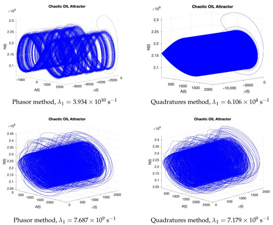
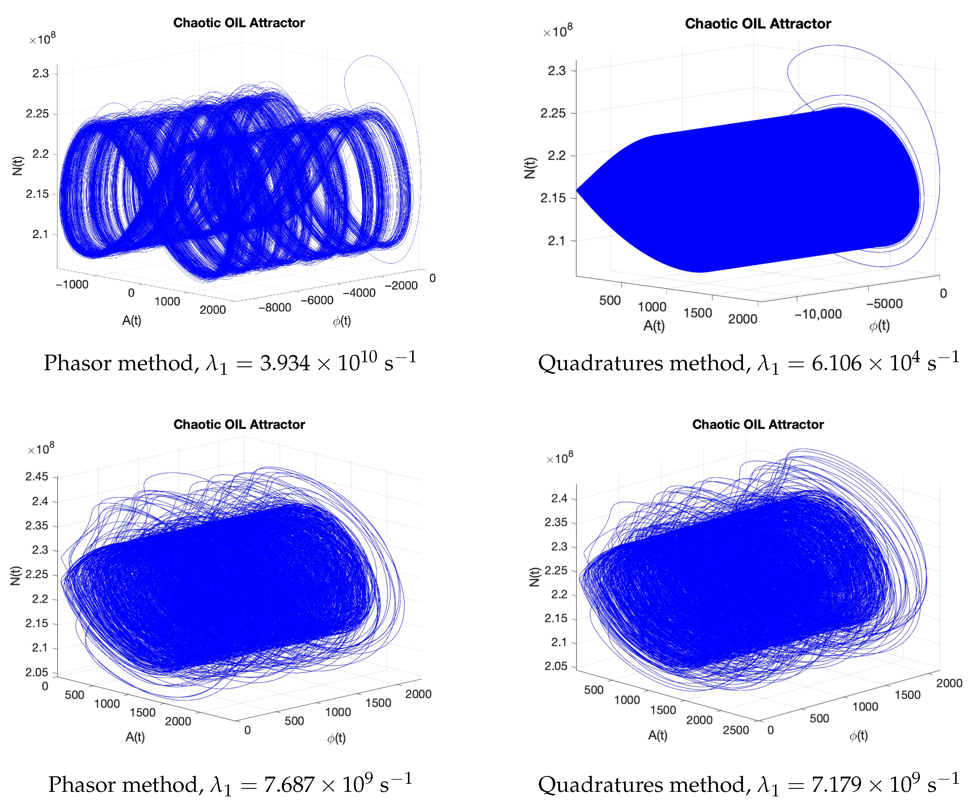
Figure 4 presents representative chaotic attractors of the master-delay-slave OIL system obtained using both the phasor and Cartesian quadrature formulations, shown side-by-side for direct comparison. All attractors are plotted in the three-dimensional phase space $\left(A\right(t),\varphi (t),N(t\left)\right)$ at a frequency detuning of $0.2$ GHz. The upper row corresponds to an injection strength of $-14$ dB, while the lower row corresponds to $-20$ dB. For each operating condition, the left side shows the attractor computed with the phasor formulation, and the right side shows the corresponding attractor obtained using the quadrature formulation.

Figure 4. Side-by-side comparison of chaotic attractors of the OIL system obtained using the phasor formulation (left column) and the Cartesian quadrature formulation (right column) plotted in three-dimensional phase space using the variables $A\left(t\right)$ (optical field amplitude), $\varphi \left(t\right)$ (optical phase), and $N\left(t\right)$ (carrier density). The trajectories exhibits bounded, aperiodic motion with intricate folding and stretching, characteristic of deterministic chaos. The attractors at the top were generated using an injection strength of $-14$ dB and a frequency detuning of $0.2$ GHz, and attractors at the bottom were generated using $-20$ dB and a frequency detuning of $0.2$ GHz, conditions under which the system displays a positive LLE.

In the Cartesian quadrature formulation the complex slave field is represented as $E\left(t\right)=X\left(t\right)+iY\left(t\right)$, from which the physically meaningful amplitude and phase can be recovered uniquely (up to the usual $2\pi$ periodicity) by the standard polar mapping

$$A\left(t\right)=\left|E\left(t\right)\right|=\sqrt{X{\left(t\right)}^2+Y{\left(t\right)}^2},\varphi \left(t\right)=arg\left(E\left(t\right)\right)=atan2\left(Y\left(t\right),X\left(t\right)\right).$$

(35)

when a continuous (unwrapped) phase trajectory is required for attractor visualization or phase-space analysis, we compute $\varphi \left(t\right)$ by unwrapping the wrapped phase $atan2(Y,X)$ in time, i.e., $\varphi \left(t\right)=\mathrm{unwrap}(atan2(Y\left(t\right),X\left(t\right)\left)\right)$, which removes the artificial $\pm \pi$ discontinuities while preserving the correct instantaneous rotation direction. This reconstruction provides a consistent bridge between the quadrature and phasor representations, enabling direct comparison of trajectories and attractors in $(A,\varphi ,N)$ coordinates while retaining the numerical robustness of the $(X,Y,N)$ dynamics.

In all cases, the trajectories remain bounded while densely filling a finite region of phase space with a thick, cloud-like structure generated by repeated stretching and folding, consistent with a strange attractor and exponential sensitivity to initial conditions. The carrier density $N\left(t\right)$ remains confined to a relatively narrow interval, reflecting the slow-fast nature of class-B semiconductor lasers, whereas the field variables explore broader ranges, revealing strong nonlinear phase-amplitude coupling and energy exchange under optical injection conditions. The attractors obtained using the quadrature formulation exhibit the same global geometry and qualitative features as those obtained using the phasor formulation, confirming that both coordinate representations produce dynamically equivalent chaotic solutions when implemented consistently.

Minor differences in local density and trajectory smoothness can be observed between the two formulations, particularly near low-amplitude regions where the phasor representation is more sensitive to numerical effects associated with $1/A$ and $1/A^2$ terms. Nevertheless, the overall phase-space structure, boundedness, and aperiodic filling remain indistinguishable, in full agreement with the positive dominant Lyapunov exponent obtained from the variational QR analysis. This consistency provides a direct visual confirmation that the chaotic dynamics identified in the Lyapunov maps correspond to genuine deterministic strange attractors and are not artifacts of a particular coordinate representation. It should be noted that negative values of the field amplitude $A\left(t\right)$ in the phasor formulation do not represent negative optical intensity; rather, they are mathematically equivalent to a $\pi$ phase shift of the complex optical field and therefore leave all physical observables unchanged.

4. Discussion and Future Research

The present study deliberately removes spontaneous emission and Langevin noise in order to isolate the intrinsic deterministic dynamics of the optically injected laser and to obtain reproducible Lyapunov spectra and chaos maps. This deterministic formulation allows the boundaries between stable, quasi-periodic, and chaotic regimes to be identified unambiguously and ensures that positive Lyapunov exponents originate from genuine nonlinear instabilities of the governing rate equations rather than from stochastic fluctuations. The resulting maps should therefore be interpreted as baseline stability diagrams of the underlying dynamical system.

In realistic experimental implementations, stochastic perturbations are always present and may blur fine stability boundaries or broaden spectral features. Nevertheless, previous experimental and numerical studies of optically injected semiconductor lasers have shown that strongly developed chaotic regimes typically persist at moderate noise levels, whereas only marginal regions near stability transitions are significantly affected. Consequently, the robust chaotic domains identified here-characterized by consistently positive dominant Lyapunov exponents and high values of $p_{\mathrm{pos}}$ are expected to maintain their qualitative integrity in practical systems. A detailed stochastic analysis, including spontaneous emission noise and technical fluctuations, lies beyond the scope of this work but represents a natural extension for future comparison with experimental realizations.

The comparison between the largest Lyapunov exponent, Kaplan-Yorke dimension, and dissipativity maps becomes fully consistent once both coordinate formulations are considered simultaneously. When computed using the Cartesian quadrature formulation, the three indicators reveal a coherent and physically consistent organization of the chaotic regions across the injection-detuning parameter space. In particular, the quadrature-based maps confirm that the dominant chaotic structures are governed primarily by injection strength and frequency detuning, while the fiber delay produces only localized modifications through its role as a phase offset in the injected field.

A key outcome of the present comparative analysis is that the quadrature formulation eliminates the appearance of spurious chaotic regions that arise in the phasor representation. In the phasor formulation, the presence of terms proportional to $1/A$ and $1/A^2$ introduces numerical sensitivity when the field amplitude approaches small values. These divisions can artificially amplify numerical noise in the variational equations and generate isolated “chaotic tongues” that are not reproduced in the quadrature formulation. Because the Cartesian system $(X,Y,N)$ avoids any division by the optical amplitude, its Jacobian remains well behaved over the entire trajectory, including low-amplitude excursions. As a result, the quadrature-based Lyapunov maps provide a more reliable and numerically robust representation of the true deterministic dynamics of the optically injected laser system.

Once the spurious numerical structures associated with the phasor formulation are removed through the Cartesian quadrature implementation, the remaining chaotic regions display a clear and physically interpretable organization. In the injection-strength interval between approximately $-13$ and $-16$ dB and frequency detuning between 0 and $0.5$ GHz, the largest Lyapunov exponent maps obtained with the quadrature formulation exhibit small but consistently positive values, indicating the presence of weak deterministic chaos. In this region the Kaplan-Yorke dimension remains relatively low and the dissipativity approaches zero, revealing a nearly balanced regime in which phase-space expansion along the unstable direction is almost compensated by contraction along the stable ones. The resulting attractor is thin and dynamically organized, corresponding to weak yet persistent chaotic oscillations governed primarily by the intrinsic carrier-photon interaction rather than by numerical artifacts.

A different dynamical balance emerges in the region between approximately $-17$ and $-24$ dB and frequency detuning between 0 and $1.7$ GHz. In this interval the dominant Lyapunov exponent remains clearly positive in the quadrature maps, confirming the persistence of deterministic chaos, while the Kaplan-Yorke dimension reaches its largest values, indicating the highest effective attractor dimensionality. Simultaneously, the dissipativity map becomes strongly negative,

$${\lambda }_1+{\lambda }_2+{\lambda }_3<0,$$

signaling a strongly dissipative regime in which global contraction dominates even though local stretching persists. Physically, this corresponds to a thicker and more dissipative chaotic attractor embedded within a rapidly contracting phase-space volume. The coexistence of a positive dominant exponent with strong global contraction produces chaotic motion that is dynamically rich yet strongly damped, in contrast to the balanced weakly chaotic regime observed at higher injection levels. The quadrature formulation therefore reveals a consistent and artifact-free organization of chaotic domains, confirming that the previously observed irregular structures were numerical in origin rather than intrinsic to the laser dynamics.

The quadrature formulation confirms that both chaotic regimes are intrinsic features of the laser dynamics rather than numerical artifacts. By providing a formulation free of amplitude singularities, the quadrature-based analysis establishes a numerically reliable reference against which the phasor representation can be assessed. The close agreement between both formulations in the main chaotic domains, together with the disappearance of isolated chaotic tongues in the quadrature maps, demonstrates that those previously observed discrepancies originate from numerical sensitivity rather than from genuine physical mechanisms.

Further work should also explore the relationship between Lyapunov-based chaos indicators and practical performance metrics in photonic applications, including chaos bandwidth, entropy rate, and randomness quality for optical random number generation. Establishing quantitative links between balanced or strongly dissipative chaotic regimes and measurable performance metrics would provide a direct bridge between nonlinear dynamical analysis and device-level optimization.

Future research should focus on extending this deterministic framework toward experimentally realistic conditions. In particular, evaluating the robustness of the quadrature-based chaotic regions under spontaneous emission noise and Langevin perturbation conditions will be essential for assessing their persistence in physical devices. Because the present results isolate the intrinsic nonlinear dynamics of the system, they provide a baseline against which noise-induced broadening or suppression of chaotic regions can be systematically quantified.

Another important direction involves extending the present comparison to systems with genuine delayed feedback, such as external-cavity semiconductor lasers, where the delay introduces additional dynamical degrees of freedom and can lead to hyperchaos and high-dimensional attractors. Such systems would provide a natural testbed for assessing the numerical robustness of different coordinate formulations in higher-dimensional dynamical settings.

Finally, experimental validation of the Lyapunov-based maps, Kaplan-Yorke dimensions, and dissipativity landscapes remains a crucial step. The quadrature-based formulation presented here offers a reliable computational framework that can be directly compared with experimentally reconstructed phase trajectories and time-series measurements, thereby strengthening the role of optically injected semiconductor lasers as controllable and reproducible sources of deterministic chaos for advanced photonic technologies.

5. Conclusions

The dynamical behavior of optically injected semiconductor lasers spans a wide range of regimes, including stable, periodic, quasi-periodic, and chaotic states, arising from the nonlinear interaction between the injected optical field and the intrinsic carrier-photon dynamics of the slave laser. By systematically varying injection strength and frequency detuning, these regimes can be accessed and controlled, enabling a detailed exploration of the bifurcation structure governing the system.

The primary motivation of this work has been to establish a physically consistent and numerically reproducible framework for Lyapunov-based chaos analysis in optically injected semiconductor lasers and, in particular, to provide a direct comparison between phasor and Cartesian quadrature formulations of the governing rate equations. Using a refined noise-free deterministic model, the largest Lyapunov exponent and the complete Lyapunov spectrum were computed through variational integration of the nonlinear equations together with their Jacobian, combined with QR-based orthonormalization. This approach avoids phase-space embedding and provides high numerical accuracy for continuous-time laser models.

The comparative analysis demonstrates that both phasor and quadrature representations yield consistent Lyapunov spectra and global chaos maps when implemented with algebraic and numerical consistency. However, the quadrature formulation eliminates amplitude singularities and resolves localized numerical artifacts observed in the phasor representation, thereby improving the robustness of chaos detection in low-amplitude regions of parameter space. The resulting Lyapunov, Kaplan-Yorke, and dissipativity maps provide a geometrically consistent description of the attractor landscape and clearly delineate transitions between stable, weakly unstable, and fully chaotic regimes as control parameters are varied. Across the explored parameter ranges, injection strength and detuning are confirmed as the dominant factors shaping the global organization of chaotic domains, while fiber forward delay primarily induces localized modulations without altering the overall topology.

The deterministic formulation adopted here isolates the intrinsic nonlinear mechanisms responsible for chaos formation and provides a strictly reproducible reference framework. Nevertheless, real semiconductor lasers are subject to spontaneous emission and other stochastic perturbations that may blur fine-scale structures near stability boundaries. While strongly chaotic regions are expected to remain structurally stable under moderate noise conditions, future work should incorporate stochastic terms and experimental validation to assess the persistence of the identified regimes under realistic operating conditions. Additional directions include quantitative evaluation of chaos bandwidth and entropy rate for photonic random-number generation, exploration of larger delay ranges and multi-laser configurations, and extension of the comparative framework to integrated photonic implementations.

Overall, the methodology developed in this study establishes a rigorous and transparent reference for Lyapunov-based characterization of chaos in optically injected semiconductor lasers. By clarifying the numerical consistency between coordinate representations and providing high-resolution dynamical maps, the present work contributes a reliable foundation for future investigations on photonic entropy generation, chaos-based secure optical communication, and the controlled exploitation of nonlinear laser dynamics in advanced photonic systems.

References

- Yu, F.; He, T.; He, S.; Tan, B.; Shi, C.; Lin, H. Influence of Memristive Activated Gradient on Chaotic Dynamics in Discrete Neural Networks. Int. J. Bifurc. Chaos 2024, 35, 2550146. [Google Scholar] [CrossRef] [Scilit]
- Yu, F.; He, S.; Yao, W.; Cai, S.; Xu, Q. Bursting Firings in Memristive Hopfield Neural Network with Image Encryption and Hardware Implementation. IEEE Trans. Comput.-Aided Des. Integr. Circuits Syst. 2025, 44, 4564–4576. [Google Scholar] [CrossRef] [Scilit]
- Feng, W.; Zhang, K.; Zhang, J.; Zhao, X.; Chen, Y.; Cai, B.; Zhu, Z.; Wen, H.; Ye, C. Integrating Fractional-Order Hopfield Neural Network with Differentiated Encryption: Achieving High-Performance Privacy Protection for Medical Images. Fractal Fract. 2025, 9, 426. [Google Scholar] [CrossRef] [Scilit]
- Li, H.; Yu, S.; Feng, W.; Chen, Y.; Zhang, J.; Qin, Z.; Zhu, Z.; Wozniak, M. Exploiting Dynamic Vector-Level Operations and a 2D-Enhanced Logistic Modular Map for Efficient Chaotic Image Encryption. Entropy 2023, 25, 1147. [Google Scholar] [CrossRef] [Scilit]
- Castañón, G.; Cerroni, W.; Sarmiento-Moncada, A.M. Integrated Photonics for IoT, RoF, and Distributed Fog–Cloud Computing: A Comprehensive Review. Appl. Sci. 2025, 15, 7494. [Google Scholar] [CrossRef] [Scilit]
- Zeng, Y.; Zhou, P.; Huang, Y.; Li, N. Optical chaos generated in semiconductor lasers with intensity-modulated optical injection:a numerical study. Appl. Opt. 2021, 60, 7963–7972. [Google Scholar] [CrossRef] [Scilit] [PubMed]
- Zhang, M.; Wang, Y. Review on Chaotic Lasers and Measurement Applications. J. Light. Technol. 2021, 39, 3711–3723. [Google Scholar] [CrossRef] [Scilit]
- Spitz, O.; Herdt, A.; Wu, J.; Maisons, G.; Carras, M.; Wong, C.W.; Elsäßer, W.; Grillot, F. Private communication with quantum cascade laser photonic chaos. Nat. Commun. 2021, 12, 3327. [Google Scholar] [CrossRef] [Scilit]
- Xie, Y.; Yang, Z.; Shi, M.; Zhuge, Q.; Hu, W.; Yi, L. 100 Gb/s coherent chaotic optical communication over 800 km fiber transmission via advanced digital signal processing. Adv. Photonics Nexus 2023, 3, 016003. [Google Scholar] [CrossRef] [Scilit]
- Wang, Z.; Shen, L.; Yang, M.; Tang, Z.; Zhang, L.; Yan, C.; Yang, L.; Wang, R.; Chu, J.; Du, J.; et al. High-speed chaos-based secure optical communications over 130-km multi-core fiber. Opt. Lett. 2023, 48, 4440–4443. [Google Scholar] [CrossRef] [Scilit]
- Feng, J.; Jiang, L.; Sun, J.; He, X.; Yi, A.; Pan, W.; Yan, L. 256 Gbit/s Chaotic Optical Communication over 1600 Km Using an AI-based Optoelectronic Oscillator Model. J. Light. Technol. 2024, 42, 2774–2783. [Google Scholar] [CrossRef] [Scilit]
- Mao, X.; Wang, A.; Wang, L.; Fu, S.; Wang, Y.; Qin, Y. 100-Gbit/s 100-km Physical-Layer Secure Fiber-Optic Communication Using Wideband Chaotic Semiconductor Lasers. J. Light. Technol. 2025, 43, 2176–2183. [Google Scholar] [CrossRef] [Scilit]
- Wang, A.; Wang, J.; Jiang, L.; Wang, L.; Wang, Y.; Yan, L.; Qin, Y. Experimental demonstration of 8190-km long-haul semiconductor-laser chaos synchronization induced by digital optical communication signal. Light Sci. Appl. 2025, 14, 40. [Google Scholar] [CrossRef] [Scilit]
- Aldaya, I.; Campuzano, G.; Castañón, G.; Gosset, C.; Wang, C.; Grillot, F. Periodic and aperiodic pulse generation using optically injected DFB laser. Electron. Lett. 2015, 51, 280–282. [Google Scholar] [CrossRef] [Scilit]
- Wieczorek, S.; Krauskopf, B.; Simpson, T.; Lenstra, D. The dynamical complexity of optically injected semiconductor lasers. Phys. Rep. 2005, 416, 1–128. [Google Scholar] [CrossRef] [Scilit]
- Ashok, P.; Ganesh Madhan, M.; Deepiha, P.; Rimmya, C.; Piramasubramanian, S. An Efficient Chaotic Optical signal generation scheme using Gain Lever Effect in bi-section laser diodes. Opt. Commun. 2020, 475, 126202. [Google Scholar] [CrossRef] [Scilit]
- Li, X.Z.; Chan, S.C. Random bit generation using an optically injected semiconductor laser in chaos with oversampling. Opt. Lett. 2012, 37, 2163–2165. [Google Scholar] [CrossRef] [Scilit] [PubMed]
- Li, J.C.; Xiao, J.L.; Yang, Y.D.; Chen, Y.L.; Huang, Y.Z. Random bit generation based on a self-chaotic microlaser with enhanced chaotic bandwidth. Nanophotonics 2023, 12, 4109–4116. [Google Scholar] [CrossRef] [Scilit]
- Wang, X.; Zheng, T.; Jia, Y.; Huang, J.; Zhu, X.; Shi, Y.; Wang, N.; Lu, Z.; Zou, J.; Li, Y. Compact Quantum Random Number Generator Based on a Laser Diode and a Hybrid Chip with Integrated Silicon Photonics. Photonics 2024, 11, 468. [Google Scholar] [CrossRef] [Scilit]
- Shen, B.; Shu, H.; Xie, W.; Chen, R.; Liu, Z.; Ge, Z.; Zhang, X.; Wang, Y.; Zhang, Y.; Cheng, B.; et al. Harnessing microcomb-based parallel chaos for random bit generation in integrated photonics. Nat. Commun. 2023, 14, 4590. [Google Scholar] [CrossRef] [Scilit]
- Yu, Q.; Chen, H.; Sun, X.; Tan, M.; Li, Y.; Xu, Z.; Pan, S. Ultra-broadband chaotic laser and microwave ranging based on an optoelectronic oscillator. Opt. Lett. 2025, 50, 3557–3560. [Google Scholar] [CrossRef] [Scilit] [PubMed]
- Mu, X.; Yan, Z.; Yu, Y.; Yan, H.; Han, D. A tunable self-mixing chaotic laser based on high frequency electro-optic modulation. Opt. Laser Technol. 2020, 127, 106172. [Google Scholar] [CrossRef] [Scilit]
- Huang, Y.; Zhou, P.; Lau, K.; Li, N. Parallel Wideband Chaos Generation System for Advancing High-Throughput Information Processing Based on an Array of Four Distributed Feedback Lasers. ACS Photonics 2024, 11, 5012–5021. [Google Scholar] [CrossRef] [Scilit]
- Huang, Y.; Gu, S.; Feng, Y.; Yang, Y.; Xiang, S.; Zhou, P.; Li, N. Wideband chaos generation using a VCSEL with intensity modulation optical injection for random number generation. Sci. China Inf. Sci. 2024, 67, 169401. [Google Scholar] [CrossRef] [Scilit]
- Inoue, S.; Kanno, K.; Uchida, A. Prevention of Intermittent Chaos in Semiconductor Laser with Optical Feedback. In Proceedings of the 2022 Conference on Lasers and Electro-Optics Pacific Rim; Optica Publishing Group: Washington, DC, USA, 2022; pp. 1–3. [Google Scholar] [CrossRef] [Scilit]
- Rodriguez, S.; Campuzano, G.; Aldaya, I.; Castañón, G. Numerical analysis of pulsing regimes near static borders of optically injected semiconductor lasers. Appl. Opt. 2022, 61, 2634–2643. [Google Scholar] [CrossRef] [Scilit]
- Castañón, G.A.; Rodriguez, S.; Campuzano, G.; Aldaya, I. Numerical analysis of the impact of noise in pulsing regimes generated using optically injected lasers. Appl. Opt. 2025, 64, 5344–5349. [Google Scholar] [CrossRef] [Scilit] [PubMed]
- Castañón Ávila, G.A.; Aragón-Zavala, A.; Aldaya, I.; Sarmiento-Moncada, A.M. High-Resolution Chaos Maps for Optically Injected Lasers. Appl. Sci. 2025, 15, 9724. [Google Scholar] [CrossRef] [Scilit]
- Sciamanna, M.; Shore, K.A. Physics and applications of laser diode chaos. Nat. Photonics 2015, 9, 151–162. [Google Scholar] [CrossRef] [Scilit]
- Wieczorek, S.; Krauskopf, B.; Lenstra, D. A unifying view of bifurcations in a semiconductor laser subject to optical injection. Opt. Commun. 1999, 172, 279–295. [Google Scholar] [CrossRef] [Scilit]
- Sivaprakasam, S.; Shore, K. Demonstration of optical synchronization of chaotic external-cavity laser diodes. Opt. Lett. 1999, 24, 466–468. [Google Scholar] [CrossRef] [Scilit] [PubMed]
- Mirasso, C.; Colet, P.; Garcia-Fernandez, P. Synchronization of chaotic semiconductor lasers: Application to encoded communications. IEEE Photonics Technol. Lett. 1996, 8, 299–301. [Google Scholar] [CrossRef] [Scilit]
- Osinski, M.; Buus, J. Linewidth broadening factor in semiconductor lasers–An overview. IEEE J. Quantum Electron. 1987, 23, 9–29. [Google Scholar] [CrossRef] [Scilit]
- Benettin, G.; Galgani, L.; Giorgilli, A.; Strelcyn, J.M. Lyapunov characteristic exponents for smooth dynamical systems and for Hamiltonian systems; a method for computing all of them. Part 1: Theory. Meccanica 1980, 15, 9–20. [Google Scholar] [CrossRef] [Scilit]
- Skokos, C. The Lyapunov Characteristic Exponents and Their Computation; Lecture Notes in Physics; Springer: Berlin/Heidelberg, Germany, 2010; Volume 790, pp. 63–135. [Google Scholar] [CrossRef] [Scilit]
- Rosenstein, M.T.; Collins, J.J.; De Luca, C.J. A practical method for calculating largest Lyapunov exponents from small data sets. Phys. D Nonlinear Phenom. 1993, 65, 117–134. [Google Scholar] [CrossRef] [Scilit]
- Kaplan, J.; Yorke, J.A. Chaotic behavior of multidimensional difference equations. In Functional Differential Equations and Approximations of Fixed Points: Proceedings, Bonn, July 1978; Peitgen, H.O., Walther, H.O., Eds.; Springer: Berlin/Heidelberg, Germany, 1979; pp. 204–227. [Google Scholar]
Disclaimer/Publisher’s Note: The statements, opinions and data contained in all publications are solely those of the individual author(s) and contributor(s) and not of MDPI and/or the editor(s). MDPI and/or the editor(s) disclaim responsibility for any injury to people or property resulting from any ideas, methods, instructions or products referred to in the content. |
© 2026 by the authors. Licensee MDPI, Basel, Switzerland. This article is an open access article distributed under the terms and conditions of the Creative Commons Attribution (CC BY) license.