Agricultural Carbon Flux Estimation Using Multi-Source Remote Sensing and Ensemble Models

Abstract

To accurately understand and investigate carbon fluxes in cropland ecosystems, this study adopted a machine learning ensemble model for estimation. Focusing on the Jinzhou station of the ChinaFLUX, we integrated eddy covariance carbon flux observations with multi-source satellite remote sensing data to construct a machine learning-based cropland carbon flux estimation model. For environmental driver selection, a strategy combining correlation analysis with ecological mechanism understanding was employed to screen LST, NDVI, and NDMI as model input variables, effectively avoiding multicollinearity issues. Using footprint-weighted integrated data from 2005 to 2014 for model training and validation, a Stacking ensemble model was constructed with the RF model serving as the meta-learner to stack the predictions of RF, CART, and GBM. The ensemble model further reduced the prediction error (RMSE = 39.82), maintaining an R² > 0.9 in most years and effectively improving predictive performance during anomalous years where single models underperformed. Based on these findings, the model was applied to analyze the spatiotemporal evolution of NEE in Jinzhou croplands from 2005 to 2014. The analysis revealed that while the region functioned overall as a carbon sink, it exhibited significant spatiotemporal heterogeneity. Spatially, the distribution followed a pattern of “strong intensity in the northeast and center, and weak intensity in the northwest and southwest.” Temporally, the sink intensity underwent significant interannual oscillations characterized by a “strengthening–weakening–re-strengthening–declining” trajectory. The high-precision prediction method proposed in this study is of great significance for revealing spatiotemporal variations in carbon sources/sinks, guiding green agricultural development, and supporting relevant policy formulation.

1. Introduction

With the increasing severity of global climate change, the carbon cycle and its impact on the environment have become a major focus of both the international academic community and the public [1,2]. The carbon cycle not only influences climate change processes but is also closely related to global energy sustainability and ecosystem development. As a key component of terrestrial ecosystems, farmland ecosystems serve as both carbon sinks and sources [3]. Through photosynthesis and soil organic carbon storage, they act as carbon sinks, while certain agricultural activities such as plowing, fertilization, and irrigation can lead to greenhouse gas emissions [4,5]. Therefore, precise quantification of farmland carbon flux is essential for understanding the spatiotemporal variations in carbon sources and sinks [6]. By quantitatively analyzing carbon flux changes in farmland ecosystems, the absorption and release patterns of carbon under different regions, crop types, and management practices can be better understood, providing a scientific basis for farmland carbon management [7,8].

Carbon in farmland ecosystems exists in different carbon pools, including the atmosphere, soil, rocks, and plants, and moves between these pools in various forms, forming carbon flux [9]. In ecological and carbon cycle research, a series of parameters are commonly used to describe and quantify the transformation and movement of carbon within ecosystems [10]. These parameters include Net Ecosystem Exchange (NEE), Ecosystem Respiration (RE), and Gross Primary Productivity (GPP), of which, NEE is used to represent the net carbon dioxide exchange between the ecosystem and the atmosphere. When NEE is positive, it indicates that carbon dioxide is emitted from the terrestrial ecosystem into the atmosphere, which means that the terrestrial ecosystem is the carbon source, and NEE represents the net carbon emission. When NEE is negative, it indicates that the terrestrial ecosystem absorbs carbon dioxide from the atmosphere and becomes a carbon sink, with NEE representing the net carbon sequestration. The NEE index can be used to quantify the carbon budget process of the ecosystem and evaluate its ecological service function in regulating climate [11]. Traditional carbon cycle research methods primarily rely on eddy covariance techniques to directly measure carbon and water fluxes between terrestrial ecosystems and the atmosphere. However, these methods are limited by terrain conditions and site deployment constraints, making them feasible only for localized and small-scale monitoring [12]. Additionally, large data gaps and poor spatiotemporal continuity present significant challenges [13], preventing continuous monitoring of farmland ecosystem carbon flux. In contrast, remote sensing technology offers wide observation coverage, short revisit cycles, high spatial resolution, broad spectral range, and high operational efficiency [14]. These advantages make remote sensing a highly promising tool for achieving continuous spatiotemporal monitoring of farmland ecosystem carbon flux.

Net Ecosystem Exchange (NEE) is a major driving factor in atmospheric CO₂ concentration changes. The application of remote sensing data has introduced new perspectives for the development of respiration models. Remote sensing indices such as Enhanced Vegetation Index (EVI), Normalized Difference Vegetation Index (NDVI), and Normalized Difference Water Index (NDWI) can reflect ecosystem environmental conditions to a certain extent [15]. During the germination, growth, and maturation stages of crops, variations in natural factors such as temperature, moisture, and light influence the overall carbon exchange within the ecosystem [16,17]. Monitoring these changes is crucial for studying ecosystem stability, climate variability, and terrestrial ecosystem cycles [18]. Some researchers have used flux observations and data assimilation methods to estimate model parameters and optimize models for generating grid-based regional carbon flux estimates [19,20,21]. However, these studies primarily analyze spatial patterns and temporal variations, without directly applying the models to carbon flux calculations [22,23]. In recent years, machine learning methods based on satellite remote sensing technology have been widely applied in ecosystem carbon cycle research. Improvements in observation techniques and the integration of remote sensing data have enhanced the availability of flux data, making the accurate quantification of ecosystem carbon flux increasingly feasible [24,25,26]. Wagle et al. [27] compared CO₂ flux in winter wheat fields under different tillage and grazing management practices using an eddy covariance system combined with remote sensing technology. By incorporating remote sensing vegetation indices, they explained the variability of CO₂ flux between different sites. Richardson et al. [28] evaluated the accuracy of 14 terrestrial biosphere models in simulating vegetation phenology, revealing deficiencies in existing models and providing insights for improving model structure and parameterization. Wu et al. [9] proposed a farmland ecosystem carbon flux estimation method based on multi-source Landsat remote sensing data. Their study found that the Random Forest model outperformed Ridge Regression and Lasso models in carbon flux estimation. However, their research lacked long-term scale assessments and high spatiotemporal resolution predictions. Additionally, they did not apply a multidimensional ensemble model, highlighting the need for further evaluation and improvement.

This study employs machine learning methods to integrate carbon flux data from the farmland ecosystem flux observation station in Jinzhou, Liaoning Province, with key environmental variables derived from multi-source remote sensing data. A farmland ecosystem carbon flux estimation method was developed using an ensemble model based on remote sensing data and machine learning. The ensemble model captures complex relationships in the carbon cycle, enhancing the spatiotemporal accuracy of carbon flux predictions and forecasting the temporal and spatial variations in farmland ecosystem carbon flux. This approach provides an innovative tool for carbon flux monitoring and offers scientific support for addressing global climate change and optimizing farmland management.

2. Data and Methods

2.1. Study Area

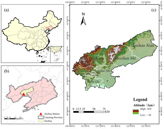
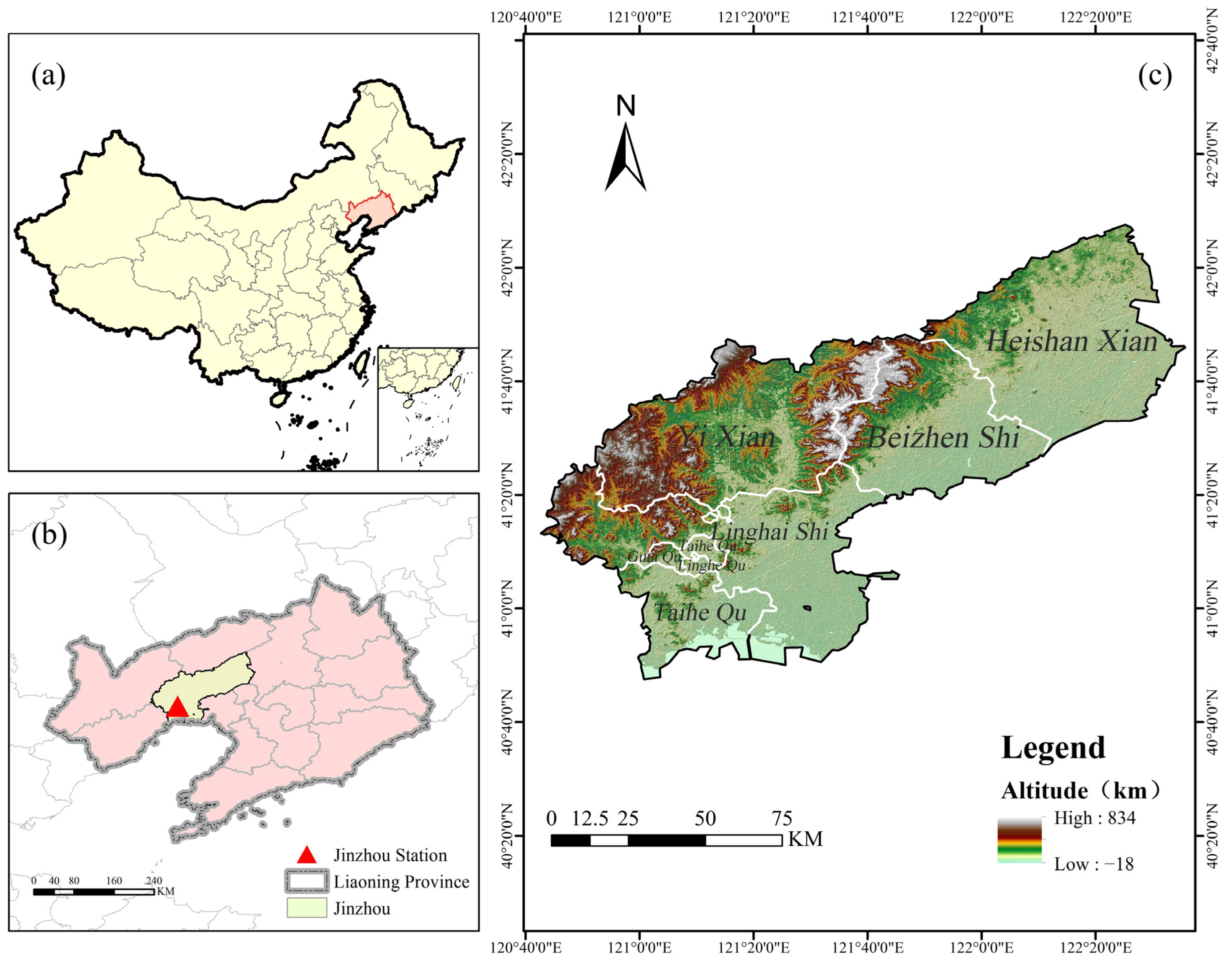
The study area is located in Jinzhou City, Liaoning Province, with the flux observation site being the ChinaFLUX Jinzhou Farmland Ecosystem Field Observation Station (121°12′6” E, 41°8′53” N). The study area has a warm temperate monsoon climate, with an average temperature of 9.5 °C and an annual precipitation of about 565.9 mm, of which 60–70% is concentrated in summer, making it suitable for agricultural production. The area is located in the “low hills and middle hills dry farming area of western Liaoning”, which is a typical agricultural and pastoral intertwined zone where dry farming and facility agriculture coexist, and the main crops grown on the farmland are corn and soybeans. The geographical location and relevant site information are shown in Figure 1 and Table 1.

Figure 1. Elevation of Jinzhou City, Liaoning Province, and the spatial distribution of the Jinzhou Farmland Ecosystem Field Observation Station. (a) Location of Liaoning Province in China. (b) Spatial distribution map of the Jinzhou Farmland Ecosystem Field Observation Station. (c) Elevation map of Jinzhou City, Liaoning Province.

Table 1. Basic Information of the Jinzhou Farmland Ecosystem Field Observation Station.

Station	Jinzhou
Longitude/(°E)	121.12
Latitude/(°N)	41.8
Soil Type	Brown Soil
Data Period	2005–2014

2.2. Data Source

2.2.1. Flux Station Data

This study leverages eddy covariance-derived carbon and water flux datasets retrieved from the National Ecosystem Science Data Center (https://www.nesdc.org.cn). Specifically, we analyzed a comprehensive time series from the Jinzhou Farmland Ecosystem Field Observation Station (1 January 2005–31 December 2014), encompassing temporal resolutions ranging from 30 min intervals to daily, monthly, and annual aggregates. Complementing this dataset, we incorporated monthly-scale flux observations obtained from the Nanjing University Jurong Ecological Experimental Station, covering the period from 1 January 2015 to 30 December 2020 [29,30]. This study mainly uses monthly carbon and water flux data for follow-up studies. The carbon-water flux indicators include Net Ecosystem CO₂ Exchange (NEE), Ecosystem Respiration (RE), Gross Primary Productivity (GPP), and Ecosystem Heterotrophic Respiration (Reco). The data processing is strictly based on the standardized technical flow system developed by ChinaFLUX for the complete process of cleaning, calibration, quality control and gap filling, which includes the following: standard preprocessing operations such as outlier removal, coordinate rotation, frequency response correction, WPL correction and steady-state tests for the original 10 Hz high-frequency data; in data quality control, the 30 min scale flux data are filtered based on the nighttime friction wind speed threshold, rainfall periods and turbulence characterization to ensure that the data used meet the turbulent exchange assumptions. In terms of data quality control, based on the nighttime frictional wind speed threshold, rainfall period exclusion and turbulence characterization, the 30 min scale flux data are filtered to ensure that the data meet the turbulent exchange assumptions. At the same time, to address the lack of measurements in sensible heat fluxes (Hs), latent heat fluxes (LE), and NEE, the data are modeled using linear interpolation, nonlinear multiple regression, marginal distribution sampling, and ecological functions to interpolate the data in stages, with a time window set to control the interpolation accuracy at different time periods. To ensure the scientific validity and comparability of the study data, the data were analyzed for energy closure, and the annual-scale fluxes were estimated using the Monte Carlo method to evaluate the data interpolation.

2.2.2. Remote Sensing Data

Carbon flux in farmland ecosystems is driven by multiple factors, including climate, vegetation, and soil [1]. Among them, satellite remote sensing technology can efficiently extract key parameters and provide spatiotemporally continuous data support for carbon flux model prediction. In this study, land surface temperature (LST) was selected as the climatic variable. For vegetation properties, the selected indices included the Normalized Difference Vegetation Index (NDVI), Difference Vegetation Index (DVI), Enhanced Vegetation Index (EVI), and Ratio Vegetation Index (RVI). For soil properties, the selected indices were the Nitrogen Reflectance Index (NRI), Normalized Difference Water Index (NDWI), and Normalized Difference Moisture Index (NDMI). These remote sensing factors were used to analyze carbon flux in farmland ecosystems [31], as shown in Table 2.

Table 2. Vegetation Indices.

	Vegetation Index	Calculation Formula
Vegetation Properties	Normalized Difference Vegetation Index (NDVI)	NDVI = (RNIR − RRed)/(RNIR + RRed)
	Difference Vegetation Index (DVI)	DVI = RNIR − RRed
	Enhanced Vegetation Index (EVI)	EVI = 2.5(RNIR − RRed)/(RNIR + 6RRed − 7.5RBlue + 1)
	Ratio Vegetation Index (RVI)	RVI = RRed/RNIR
Soil Properties	Nitrogen Reflectance Index (NRI)	NRI = (RGreen − RRed)/(RGreen + RRed)
	Normalized Difference Water Index (NDWI)	NDWI = (RGreen − RNIR) (RGreen + RNIR)
	Normalized Difference Moisture Index (NDMI)	NDMI = (RNIR − RSWIR1)/(RNIR + RSWIR1)

We selected the MODIS/Terra MOD11A1 Version 6 and the MODIS Surface Reflectance Daily L2G Global 500m (MOD09GA) satellite remote sensing data product to calculate climate, vegetation, and soil indices [32,33]. MOD09GA is a daily value product of surface reflectance (SR) from the moderate resolution imaging spectrometer (MODIS) provided by NASA, including Red (620–670 nm), near-infrared (NIR:841–876 nm), Blue (459–479 nm), Green (545–565 nm), and shortwave infrared (SWIR1: 1230–1250 nm, SWIR2: 1628–1652 nm, SWIR3: 2105–2155 nm) [34]. As a Level 2G product, MOD09GA undergoes rigorous atmospheric and geometric corrections and includes a quality control (QC) band. With its high temporal and spatial resolution, MOD09GA can effectively capture vegetation phenological dynamics and the instantaneous spectral responses to extreme weather events, thereby providing key spatiotemporally continuous driving parameters for carbon flux modeling. Furthermore, to achieve strict spatiotemporal alignment between the LST data and the MOD09GA product, the nearest neighbor interpolation method was employed to resample the resolution from 1 km to 500 m.

This research is based on the Google Earth engine (GEE) cloud platform (https://code.earthengine.google.com/). After obtaining the MODIS (MOD09GA) remote sensing data of the study area from 2005 to 2014, the quality control (QC) band was used for cloud mask processing to eliminate the low-quality pixels affected by cloud layers, cloud shadows, aerosols and other factors. Then, the maximum value composite (MVC) method was used to synthesize the time-series data to generate high-quality datasets without clouds or missing values. After radiometric correction and geometric correction, the vegetation indices were further calculated using the corrected band data for subsequent analysis.

2.3. Methods

2.3.1. Spatial Alignment of Flux Observations and Remote Sensing Data

Given that the source area (flux footprint) of Eddy Covariance (EC) observations varies dynamically with atmospheric turbulence conditions, whereas MODIS satellite data possess a fixed pixel grid (500 m), there exists an inherent spatial-scale mismatch between the two datasets. To address this issue and accurately quantify the actual representativeness of remote sensing signals for the flux observations, this study adopted the two-dimensional Flux Footprint Prediction (FFP) model proposed by Kljun et al. to construct a footprint-weighted scheme for matching satellite and tower data [35].

(1)

Dynamic Footprint Modeling

The FFP model was driven by micrometeorological data at a 30 min temporal resolution. Key input parameters included the measurement height (z_m), zero-plane displacement (d), roughness length (z₀), friction velocity (u_*), and wind direction. Consequently, a two-dimensional flux contribution function (source weight function) was derived for each observation timestamp. This function quantitatively describes the relative contribution of different upwind surface locations to the measured flux at the tower.

(2)

Footprint-Weighted Pixel Aggregation

To mitigate spatial heterogeneity errors associated with traditional single-pixel extraction or simple arithmetic averaging, the generated dynamic footprints were projected onto the MODIS pixel grid. For a given timestamp, the spatially weighted reflectance within the tower’s source area was calculated using the following equation:

$$R_{tower,t}={\displaystyle \frac{\sum _{i=1}^N (R_{i,t}\cdot w_{i,t})}{\sum _{i=1}^N w_{i,t}}}$$

where

$\mathit{N}$ represents the total number of MODIS pixels falling within the flux footprint area;

${\mathit{R}}_{\mathit{i},\mathit{t}}$ denotes the MODIS surface reflectance (MOD09GA) of the $\mathit{i}$-th pixel at time $\mathit{t}$;

${\mathit{w}}_{\mathit{i},\mathit{t}}$ corresponds to the spatially integrated footprint weight within the $\mathit{i}$-th pixel, defined as ${\mathit{w}}_{\mathit{i},\mathit{t}}={\iint }_{\mathit{p}\mathit{i}\mathit{x}\mathit{e}{\mathit{l}}_{\mathit{i}}} \mathit{\varphi }(\mathit{x},\mathit{y})\mathit{d}\mathit{x}\mathit{d}\mathit{y}$.

This approach ensures that the remote sensing signals input into the model maintain strict physical consistency with the field of view (FOV) of the flux tower observations.

2.3.2. Machine Learning Methods

The Ensemble Model is a machine learning approach that enhances overall predictive performance by combining multiple base learners, thereby improving the accuracy and stability of the model [36]. In this study, an ensemble model was constructed using the stacking method, which integrates the predictive advantages of three algorithms: Random Forest (RF), Classification and Regression Trees (CART), and Gradient Boosting Machines (GBM) to improve the robustness and accuracy of carbon flux prediction in farmland ecosystems [36]. The fundamental principle of stacking involves first building individual models with different algorithms (base learner layer) to generate diverse primary predictions. These predictions are then used as input features to train a secondary model (meta-learner layer), which produces the final prediction output. The base learner layer captures the nonlinear interactions and temporal dependencies among vegetation dynamics, meteorological factors, and soil properties, while the meta-learner layer integrates the predictions of multiple models through regularization constraints, thereby suppressing overfitting and balancing the effects of spatial heterogeneity.

RF is a supervised learning algorithm based on decision trees, proposed by Leo Breiman and Adele Cutler [37,38]. The core idea of RF is to construct multiple decision trees and aggregate their predictions to make the final decision. Random Forest exhibits strong resistance to overfitting and high prediction accuracy, making it well-suited for handling high-dimensional, nonlinear, and complex data. The core formula of the Random Forest model is:

$$\widehat{\mathcal{Y}}={\displaystyle \frac{1}{\mathcal{n}}}\sum _{i=1}^n{T}_{\mathcal{i}}\left(x\right)$$

where

$\widehat{\mathcal{Y}}$ represents the final predicted value, T_i(x) denotes the prediction of the ith decision tree, and n is the total number of decision trees.

CART is a classical supervised learning algorithm first proposed by Breiman et al. in 1984 [39]. The core idea of CART is to select the optimal feature and splitting point to iteratively construct a binary decision tree by splitting nodes. This method is effective in handling nonlinear relationships, making it widely used in both classification and regression tasks. However, CART models are prone to overfitting, especially when deep trees are constructed without proper pruning. To mitigate this issue, techniques such as pruning, setting a minimum number of samples per split, and limiting tree depth are commonly employed.

$$f_m(x)=\sum _{j=1} c_{jm}\cdot I(x\in R_{jm})$$

where

$f_m\left(x\right)$ is the prediction of the m-th tree, $jm$ is the number of leaf nodes of the m-th tree, and $c_{jm}$ is the predicted value of the j-th leaf node. Since using CART alone is prone to overfitting, it is often combined with ensemble learning methods to improve prediction accuracy and generalization ability. Ensemble techniques such as Bagging, Boosting, and Stacking help mitigate overfitting by leveraging multiple models and aggregating their predictions.

GBM is an iterative machine learning algorithm that improves model performance by sequentially fitting the residual errors [40,41]. Through multiple rounds of iteration, GBM gradually enhances prediction accuracy, making it well-suited for capturing complex nonlinear relationships. The model is updated iteratively using the following equation:

$$F_m\left(x\right)=F_{\left(m-1\right)}\left(x\right)+\eta ·h_m\left(x\right)$$

where

F_m(x) is the updated model at iteration m, h_m(x) is the newly added weak learner, and η is the learning rate controlling the contribution of each tree.

2.4. Model Cross-Validation

The Leave-One-Year-Out Cross-Validation (LOYOCV) method was adopted to evaluate model performance. For the flux observation dataset spanning N complete years, the validation process consisted of N independent iterations. In each iteration, the complete data from a specific year were withheld as an independent testing set, while the data from the remaining N-1 years were aggregated to serve as the training set for model construction. This strategy ensures strict temporal isolation between the training and validation datasets. The overall model performance was assessed based on the prediction results across all validation years using the Mean Absolute Error (MAE), Root Mean Square Error (RMSE), and the Coefficient of Determination (R²). The smaller the MAE, the smaller the prediction error of the model. The smaller the RMSE, the higher the prediction accuracy of the model. The value of R² ranges from 0 to 1. The closer the value is to 1, the more the model can explain the variability of the data, and the better the model fitting effect.

3. Results

3.1. Carbon Flux and Influencing Factors of the Farmland Ecosystem

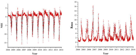
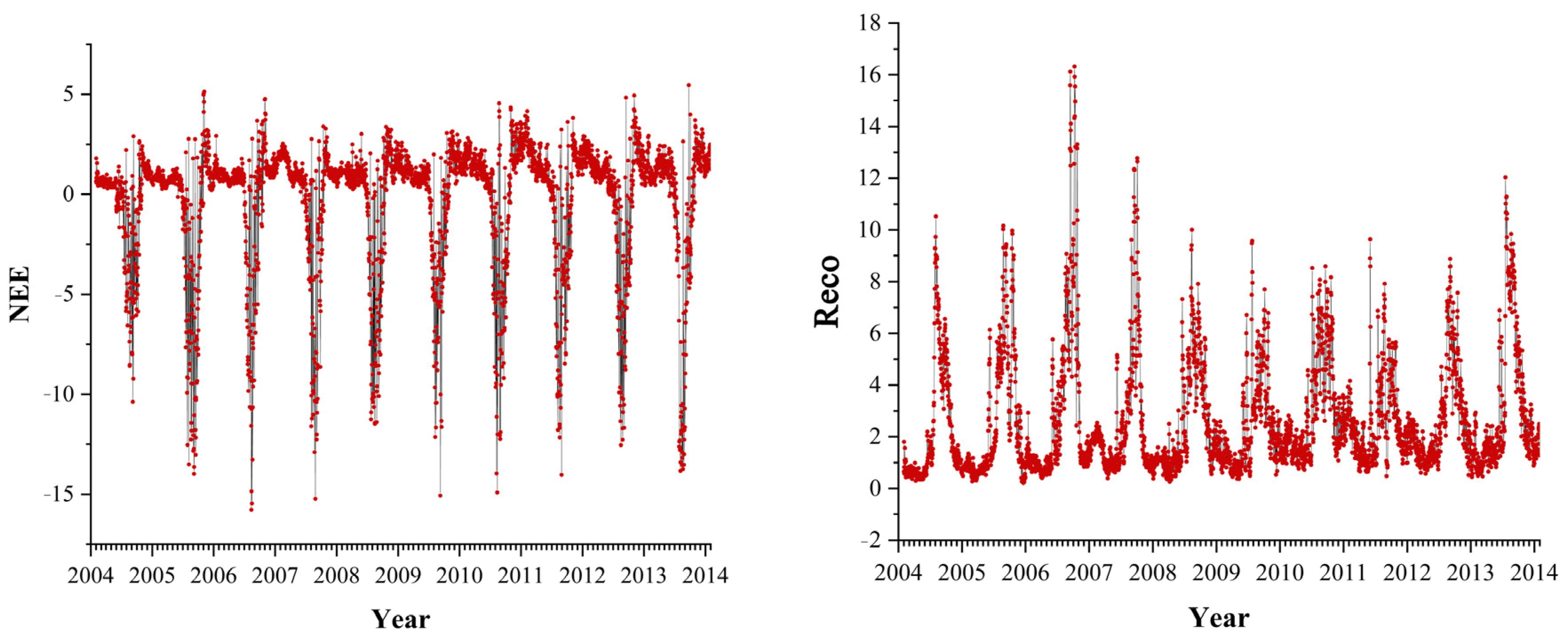
The time series of NEE and Reco carbon fluxes are shown in Figure 2. The carbon fluxes of the farmland ecosystem showed significant seasonal fluctuations, which were affected by the seasonal fluctuations of environmental factors. In addition to being regulated by environmental factors, carbon clux is also significantly related to crop growth stages. The Jinzhou flux observation field and the nearby main crop, spring maize, led to the M-shaped seasonal variation of carbon flux in the Jinzhou farmland ecosystem. NEE changed from a positive value to a negative value from the maize sowing period (April–May) to maturity period (July–August). NEE reached the extreme value at crop maturity, and the NEE of the farmland ecosystem changed from a negative value to a positive value again after the harvest of crops.

Figure 2. NEE and Reco Time Series Plots.

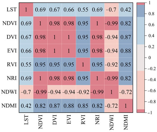
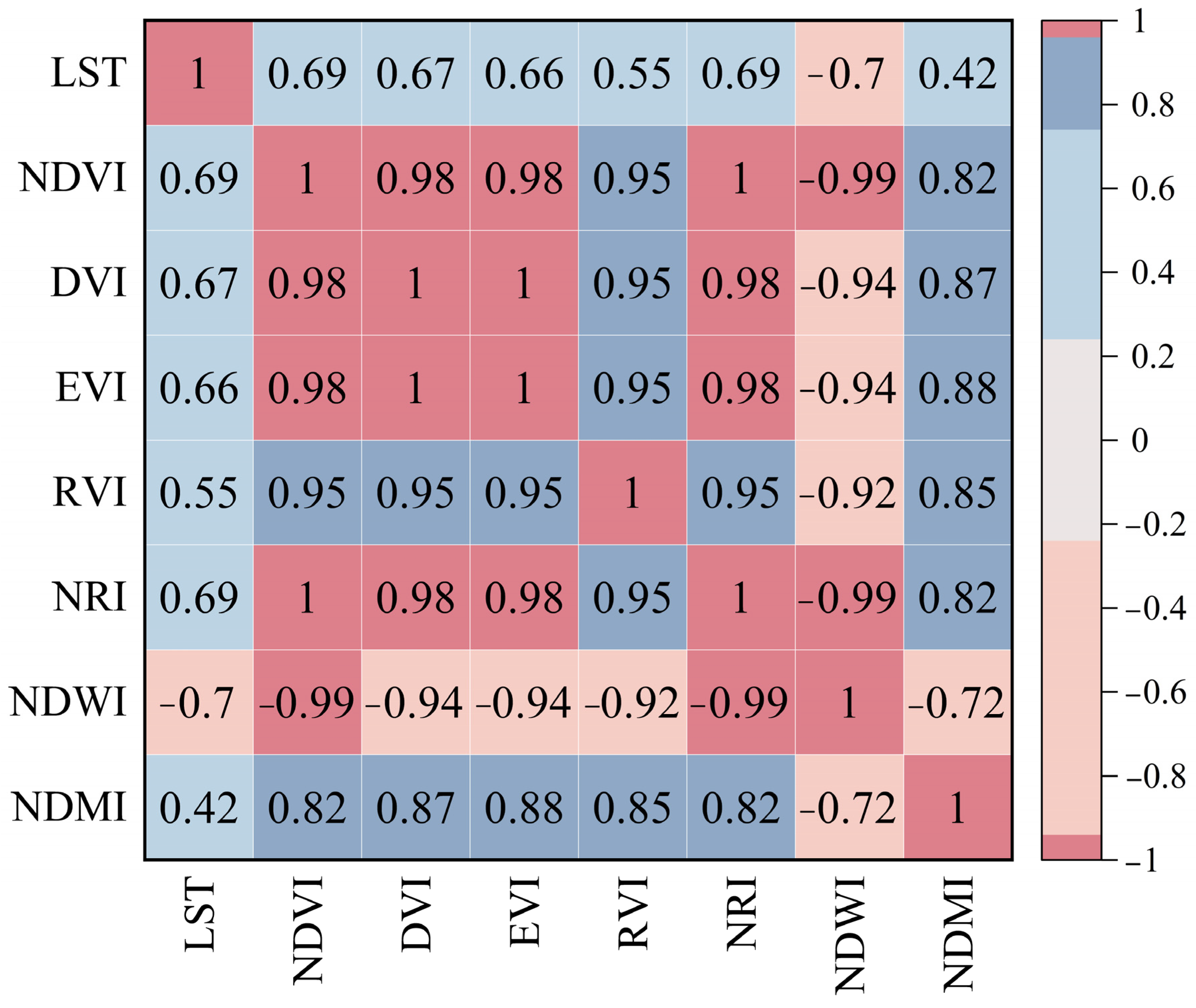
To minimize uncertainty in parameter estimation and enhance the stability and interpretability of the carbon flux prediction models, a rigorous multicollinearity diagnosis and variable selection process was conducted based on the Pearson correlation coefficient matrix of environmental factors (Figure 3). The analysis revealed extremely strong positive correlations among the vegetation indices (NDVI, DVI, EVI, RVI, and NRI), with coefficients ranging from 0.95 to 1.0. This indicates substantial information redundancy among these indices in characterizing vegetation growth. Furthermore, the correlation coefficient between NDWI and NDVI reached −0.99, suggesting that the variation information contained in both is nearly identical; thus, including both would not contribute additional effective information dimensions. Following the principles of avoiding multicollinearity and maximizing information gain, we retained NDVI due to its widespread application and clear ecological significance, while excluding the highly coupled indices (DVI, EVI, RVI, NRI, and NDWI). In contrast, LST showed a moderate correlation with NDVI (r = 0.69) and a lower correlation with NDMI. This suggests that LST and NDMI provide information on the land surface thermal environment and canopy water stress, respectively, which are distinct from vegetation greenness, thereby offering significant complementary value. Integrating considerations of statistical independence and biophysical mechanisms, LST, NDVI, and NDMI were ultimately selected as the core driving variables to construct the input dataset alongside NEE.

Figure 3. Heatmap of Correlation Coefficients of Environmental Factors.

3.2. Model Evaluation

The predictive performance of the RF, CART, GBM, and Ensemble models in estimating NEE values was quantitatively evaluated using RMSE and R², with results presented in Table 3 andTable 4. As shown in Table 3, the RF model demonstrated superior stability, with R² values exceeding 0.65 in 8 out of the 10 tested years. Specifically, the RF model achieved a peak R² of 0.968 in 2010, and high values of 0.909 and 0.906 in 2009 and 2013, respectively. In contrast, both CART and GBM models exhibited poor performance in 2005, yielding negative R² values of −0.656 and −0.139, respectively. This suggests significant predictive failure for that year, likely attributable to anomalies in sample characteristics or discrepancies in data distribution. Furthermore, in 2012, all models produced R² values below 0.65, with CART reaching only 0.432, indicating inherent difficulties in predicting NEE for that specific year. Table 4 summarizes the performance on the monthly-scale test set. The RF model achieved an average R² of 0.788 ± 0.138, outperforming CART and GBM by 0.166 and 0.092, respectively. In terms of error metrics, the RF model yielded the lowest MAE (25.25 ± 7.21) and RMSE (39.95 ± 13.67), coupled with the smallest standard deviation in R². Conversely, the CART model showed the highest instability, with an R² standard deviation of 0.473. These results indicate that the RF model possesses the highest predictive accuracy and stability among the single models. Consequently, RF was selected as the meta-learner to stack the predictions of the sub-models for generating the final Ensemble model. The Ensemble model demonstrated further improvements, achieving an RMSE of 39.82 ± 15.67, a reduction of 0.13 compared to the RF model. Notably, the Ensemble model maintained high and stable accuracy across most years, with R² values exceeding 0.9 in 2009, 2010, 2011, and 2013. Even in the anomalous year of 2005, although the R² was lower, the Ensemble model still outperformed both CART and GBM, highlighting the robustness of the stacking strategy in handling outlier data. In summary, the Ensemble model successfully integrated the strengths of multiple base models, demonstrating superior performance in terms of both accuracy and stability, thereby validating the effectiveness of the stacking ensemble learning strategy. However, to further enhance predictive precision, future research should focus on acquiring data from more observation sites, optimizing model parameters, or conducting advanced feature engineering to fully exploit latent information within the data.

Table 3. Model Prediction Annual Performance Metrics.

Year	RF	CART	GBM	Ensemble Model
2005	0.562	−0.656	−0.139	0.023
2006	0.850	0.744	0.803	0.824
2007	0.659	0.676	0.733	0.727
2008	0.756	0.696	0.669	0.721
2009	0.909	0.885	0.907	0.916
2010	0.968	0.896	0.921	0.951
2011	0.898	0.898	0.889	0.908
2012	0.643	0.432	0.470	0.506
2013	0.906	0.917	0.924	0.927
2014	0.726	0.735	0.785	0.756

Table 4. Summary Performance Metrics of Model Predictions.

	RF	CART	GBM	Ensemble Model
MAE	25.25 ± 7.21	30.95 ± 1.24	28.06 ± 8.60	27.03 ± 9.08
RMSE	39.95 ± 13.67	44.70 ± 17.60	41.22 ± 15.56	39.82 ± 15.67
R2	0.788 ± 0.138	0.622 ± 0.473	0.696 ± 0.326	0.726 ± 0.281

To rigorously evaluate the spatial generalizability of the proposed framework, the Jurong Ecological Experimental Station was designated as an independent validation site. Situated in central China, this site contrasts with the northern Jinzhou station by spanning a substantial latitudinal gradient characterized by distinct climatic regimes and vegetation types (Table 5). This marked biogeographical heterogeneity provides an optimal testbed to verify the spatial applicability of our single-site trained model. Validation against the Jurong flux observations yielded strong performance metrics (R² = 0.702, RMSE = 48.61, MAE = 32.69), demonstrating that the model retains high predictive fidelity under cross-regional application. Consequently, the model exhibits robust spatial transferability, offering a reliable methodological foundation for flux estimations across diverse ecological regions.

Table 5. Comparison of environmental characteristics between Jinzhou and Jurong stations.

Variable	Jinzhou Mean	Jurong Mean	Difference
NDVI	0.43	0.48	0.05
NDMI	0.52	0.13	0.39
LST	8.78	17.67	8.89

3.3. Spatial Distribution Characteristics of Model-Predicted Regional NEE

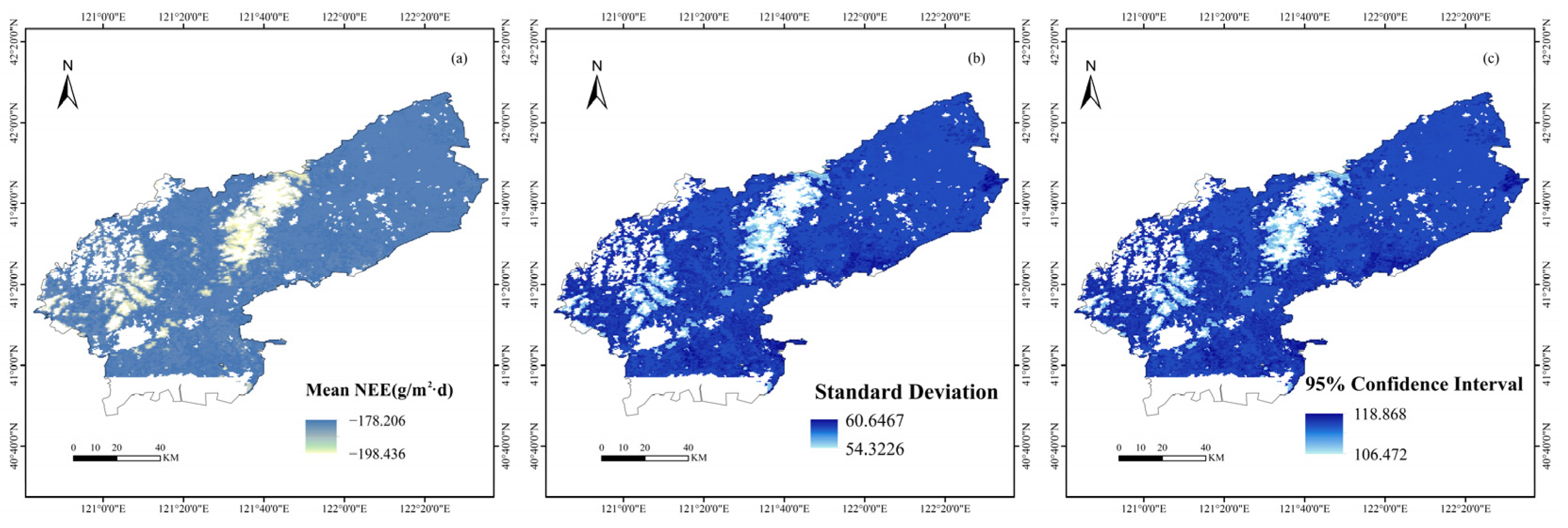
Based on the ensemble model, the spatial distribution characteristics of the Net Ecosystem Exchange (NEE) in Liaoning Province were simulated, with the results presented in Figure 4. The model outputs included three metrics: mean NEE, standard deviation, and the 95% confidence interval (CI), facilitating a comprehensive evaluation of the spatial pattern of regional carbon exchange and its associated uncertainty.

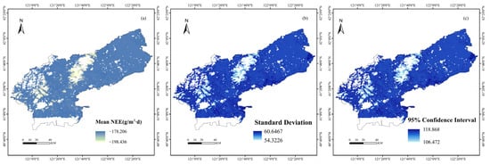
Figure 4. Spatial Distribution of Mean, Standard Deviation, and 95% CI for NEE in Jinzhou. (a) Spatial distribution of mean NEE (g/m²·d); (b) Spatial distribution of standard deviation; (c) Spatial distribution of 95% confidence interval.

Figure 4a displays the spatial distribution of the mean NEE predicted by the ensemble model. The values ranged from −198.436 to −178.206 g/(m²·d), indicating that all farmland areas functioned as carbon sinks. The carbon sink intensity exhibited significant spatial heterogeneity: the central plain and northeastern farmlands showed the highest carbon sink intensity, with NEE values approaching −198 g/(m²·d), suggesting a stronger carbon sequestration capacity in these regions. Conversely, the western and southern farmlands exhibited relatively weaker carbon sink intensity, with NEE values near −178 g/(m²·d). Overall, the farmlands in Liaoning Province demonstrated a strong carbon sink function, with a regional variation in carbon sink intensity of approximately 20 g/(m²·d). Figure 4b illustrates the spatial distribution of the standard deviation of the predicted NEE, ranging from 54.3226 to 60.6467. The spatial pattern of the standard deviation was similar to that of the mean NEE. The central and northeastern farmlands showed relatively larger standard deviations, indicating a higher degree of dispersion in model predictions for these areas; in contrast, the western and southern regions had smaller standard deviations, suggesting relatively stable predictions. Furthermore, Figure 4c presents the 95% confidence interval of the predicted NEE, with values ranging from 106.472 to 118.868. The spatial distribution pattern of the confidence interval was generally consistent with that of the standard deviation. The central and northeastern regions exhibited wider confidence intervals, exceeding 118, which indicates higher prediction uncertainty in these areas. Conversely, the western and southern regions showed relatively narrower intervals of approximately 106, implying better reliability of the model predictions.

The above integrated model, trained and verified based on the flux data of the Jinzhou farmland ecosystem field observation station and remote sensing factors, has good estimation performance, and can be used to reveal the dynamics of regional farmland carbon flux. This study further extended the application of the ensemble model to the cropland ecosystem of Jinzhou City to achieve spatial prediction of NEE. By integrating multi-source remote sensing data and meteorological data, the model performed pixel-by-pixel carbon flux estimation for the Jinzhou agricultural region, generating an NEE spatial distribution map covering the entire cropland area.

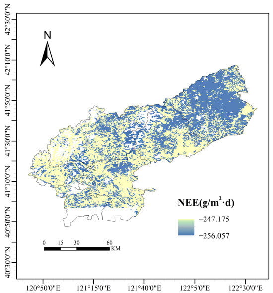
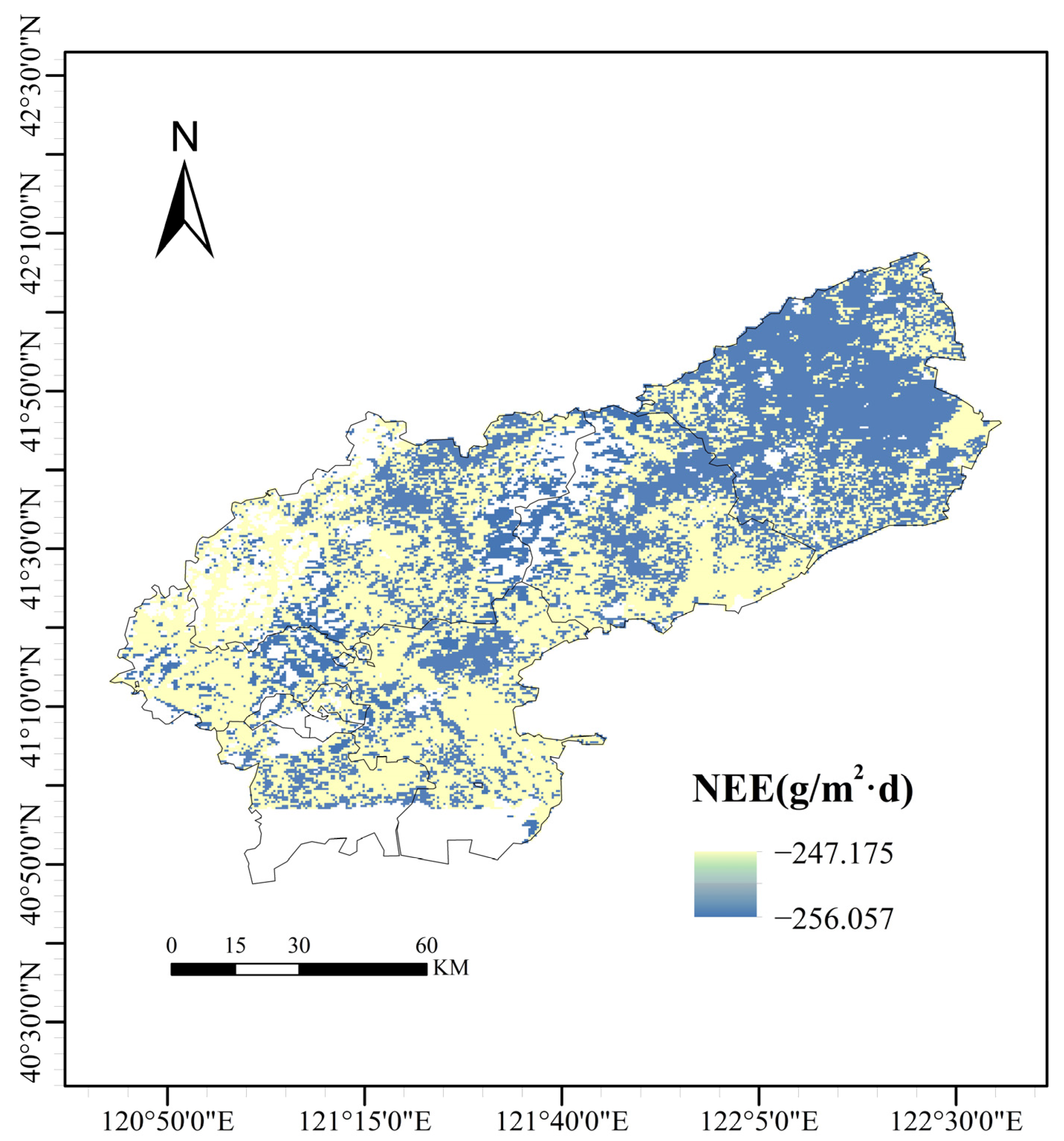
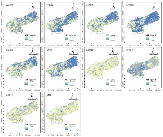
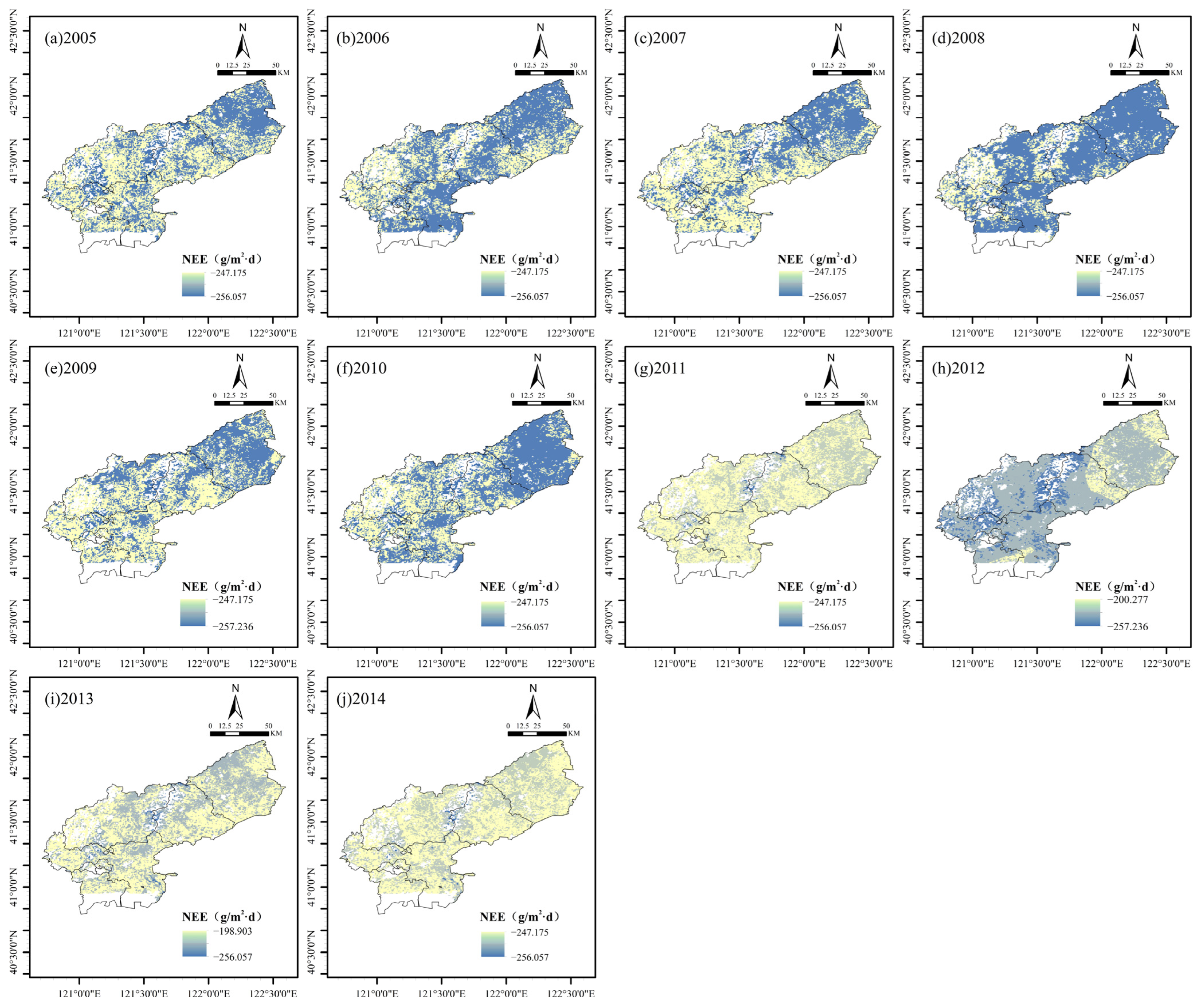
As illustrated in Figure 5, the multi-year average NEE spatial distribution from 2005 to 2014 reveals that the Jinzhou region generally exhibits a carbon sink intensity pattern characterized by “high intensity in the northeast and center, and low intensity in the northwest and southwest.” The results indicate that NEE values within the region ranged from −256.06 to −247.18 g/(m²·d). All values across the region were negative, demonstrating that the area functioned as a net carbon sink throughout the 2005–2014 period. In terms of spatial morphology, high carbon sink areas (represented by dark blue patches) displayed a relatively continuous and clustered distribution, primarily covering the northeastern hinterland and the central core of the study area, where the ecosystem carbon sequestration capacity was strongest. In contrast, low carbon sink areas (represented by light yellow patches) exhibited characteristics of fragmentation and marginalization, mainly scattered along the northwestern boundary and in parts of the southern and southwestern regions. This “patchy” mosaic structure, interlaced with dark blue and light yellow, reflects the complexity of vegetation types, soil textures, and topography within the region, suggesting that the regional carbon budget process possesses high sensitivity to the spatial heterogeneity of local environmental factors. Figure 6 further reveals the spatiotemporal evolution patterns of NEE in Jinzhou from 2005 to 2014. Spatially, the overall pattern featured lower values (stronger sink) in the northeast and center, and higher values (weaker sink) in the northwest and southern peripheries. However, from a temporal perspective, the overall carbon sink intensity of the region exhibited significant interannual fluctuations. A comparison of the year-by-year simulation results indicates that 2008 (Figure 6d) and 2010 (Figure 6f) were the years with the strongest carbon sink capacity, with the vast majority of the region appearing dark blue and showing significant negative NEE values. Conversely, 2011 (Figure 6g) and 2014 (Figure 6j) showed a marked trend of weakening carbon sink capacity; the light yellow areas expanded significantly, not only occupying the western edge but also encroaching upon the high carbon sink core zones in the center and northeast, resulting in a noticeably lighter overall tone across the region. Additionally, data for 2012 (Figure 6h) showed a wider range of value variation, with distinct low carbon sink features appearing in localized areas. Overall, while maintaining a relatively stable spatial structure, the region experienced an alternating interannual oscillation process of “strengthening–weakening–re-strengthening–declining”.

Figure 5. Spatial distribution of multi-year average NEE values in Jinzhou City (2005–2014).

Figure 6. Annual spatial patterns of NEE in Jinzhou City (2005–2014). (a) 2005; (b) 2006; (c) 2007; (d) 2008; (e) 2009; (f) 2010; (g) 2011; (h) 2012; (i) 2013; (j) 2014. NEE values are expressed in g/(m²·d).

4. Discussion

4.1. Environmental Factor Selection and Model Construction

This study employed a hybrid strategy combining correlation analysis with ecological mechanism understanding when constructing a carbon flux prediction model for agricultural ecosystems. Ultimately, three environmental variables moderately correlated with NEE—LST, NDVI, and NDMI—were selected for inclusion, rather than incorporating all available environmental factors. From a statistical perspective, including highly correlated variables simultaneously in a model can induce multicollinearity issues. This leads to unstable parameter estimates, increased standard errors, and ultimately reduces the model’s predictive reliability [42]. Previous studies typically employed two extreme approaches: either using all available variables in hopes of automatically identifying important factors through data-driven methods, or relying purely on statistical techniques like stepwise regression or LASSO regularization for variable selection [43]. The former often suffers from overfitting due to variable redundancy, while the latter, though reducing dimensionality, may sacrifice ecological interpretability. In contrast, this study’s hybrid strategy ensures both statistical robustness and ecological interpretability, effectively avoiding overfitting in flux estimation caused by excessive input variables. Ecologically, the importance of vegetation indices and surface temperature as key variables for carbon flux prediction has been confirmed by extensive eddy-correlation scale-expansion studies. Global-scale NEE estimation studies indicate that NDVI explains over 60% of GPP variation, primarily due to its strong correlation with photosynthetic active leaf area index (LAI) [44,45]. Surface temperature serves as the primary driver of ecosystem respiration (Re), significantly regulating spatiotemporal NEE variability by influencing soil microbial activity and plant autotrophic respiration [46,47]. NDMI, as an indicator of vegetation water status, provides substantial explanatory power for carbon flux changes under drought stress [48]. Thus, the three variables selected in this study are not only statistically sound but also ecologically grounded.

Through a comparative analysis of the predictive performance of three single models—RF, CART, and GBM—this study revealed that the Random Forest (RF) model demonstrated superior generalization capability and stability, achieving an R² of 0.788 and an RMSE of 39.95 in monthly-scale tests. Notably, RF successfully overcame the overfitting issues observed in CART and GBM, which yielded negative R² values in 2005. Consequently, the most stable RF model was selected as the meta-learner for the Stacking ensemble strategy, aiming to further smooth prediction errors by integrating the strengths of the sub-models. Evaluation results confirmed the effectiveness of this strategy; the Ensemble model’s RMSE decreased to 39.82, a reduction of 0.13 compared to the best-performing single model (RF). This indicates that by learning from the sub-models’ predictions, the ensemble approach effectively captures residual information that single models failed to explain. Simultaneously, the ensemble strategy significantly enhanced temporal robustness. It not only maintained excellent accuracy (R² > 0.9) in years such as 2009, 2010, and 2013 but also effectively mitigated the extreme prediction errors of base learners in 2005, thereby preventing the “bucket effect.” However, the fact that R² values for all models remained below 0.65 in 2012 suggests that current models still face bottlenecks when dealing with extreme climate events or complex environmental factors. This limitation may be attributed to the insufficient explanatory power of the feature variables for abnormal conditions. Model errors may arise from the observational uncertainty of flux data, the limitations in spatial resolution of remote sensing data, and the insufficient capture of nonlinear relationships between environmental factors and NEE. Furthermore, as this study relied solely on data from a single site for model training, the generalizability of the model to different cropland types and climatic regions remains to be further validated. Furthermore, compared to global models that seek universality across highly heterogeneous ecosystems, regional-scale specialized models can better capture the carbon cycle characteristics of specific crop types and management practices. This provides more reliable quantitative evidence for assessing agricultural carbon sink potential and optimizing emission reduction and sink enhancement technologies.

4.2. Spatiotemporal Patterns of Carbon Flux

The spatial pattern of NEE, characterized by “high values in the northeast/center and low values in the northwest/southwest” as revealed in this study, profoundly reflects the constraints imposed by underlying surface habitat conditions on the cropland carbon budget in the Jinzhou region. The pronounced high carbon sink features observed in the northeastern and central core areas are primarily attributed to the superior configuration of water and soil resources in these regions. Situated mostly on river alluvial plains, these areas possess deep soil layers with high organic matter content. Coupled with relatively well-developed irrigation facilities, these conditions provide a sufficient foundation of water and nutrients for crop photosynthesis, enabling the rate of ecosystem carbon sequestration to exceed that of respiratory consumption. Conversely, the low carbon sink patches emerging in the northwestern and southern peripheries are likely related to local topography and soil degradation. The northwest serves as a transition zone of low mountains and hills, characterized by undulating terrain and relatively weak soil water and fertilizer retention capacities. Consequently, crops in this area may face more severe water stress, which limits carbon assimilation capacity during the growing season. Meanwhile, the fragmented low-value areas along the southern edge may be subject to anthropogenic disturbances, such as urban expansion or frequent land-use conversion. These activities lead to a decline in vegetation coverage, thereby weakening the overall regional carbon sink function. The “strong-to-weak” alternating oscillation of regional NEE observed from 2005 to 2014 reveals the strong sensitivity of cropland ecosystems in the temperate semi-humid monsoon zone to hydrothermal factors. The emergence of 2008 and 2010 as strong carbon sink years was mainly due to the significant “synchronization of water and heat.” During these years, abundant precipitation in the growing season was highly matched with suitable accumulated temperatures, which maximized the photosynthetic potential of crops and promoted rapid biomass accumulation. However, the significant decline in carbon sink function in 2011 and 2014 reflects the negative effects of extreme climate events or hydrothermal imbalances. In years characterized by insufficient precipitation or high-temperature drought, crops subjected to water stress are induced to close stomata to reduce transpiration, which directly inhibits photosynthesis. Simultaneously, high temperatures may accelerate soil heterotrophic respiration. This dual effect of “reduced carbon uptake and increased carbon emission” resulted in a decrease in the magnitude of negative NEE values (i.e., a weaker sink). Furthermore, the high spatial variability of NEE in 2012 suggests an extremely uneven spatial distribution of climatic conditions that year, possibly involving localized meteorological disasters that caused drastic divergence in crop growth status across different areas. This indicates that despite the strong artificial management attributes of cropland ecosystems, they still exhibit significant vulnerability when confronting interannual climate fluctuations. This pattern is consistent with findings from other studies within China’s Agricultural Carbon Monitoring Network. For instance, Zhang et al. [49] found through a comprehensive analysis of multi-site data from the ChinaFLUX that agricultural ecosystems in the North China Plain typically function as net carbon sinks during the crop growing season. This study extends the conclusions of these point observations to a spatial scale, demonstrating that the carbon sink characteristics observed at single points are representative at the regional scale. This provides empirical support for scaling up from flux tower observations to regional carbon budget assessments. However, the finding of spatial homogeneity in carbon sink capacity contrasts sharply with studies of natural ecosystems, revealing the unique ecological effects of agricultural management. Baldocchi et al. [50], synthesizing data from the global FluxNet network, indicates that forest ecosystems exhibit significant spatial heterogeneity in carbon sequestration capacity, strongly influenced by natural factors such as topography, soil type, and species composition. Reichstein et al. [51] similarly observed high spatial heterogeneity in European grassland ecosystems, where carbon fluxes are complexly regulated by precipitation gradients, soil fertility, and species diversity. In contrast, the spatially uniform distribution pattern of agricultural carbon sinks identified in this study demonstrates humanity’s capacity to shape ecosystem functions. Within the study area, uniform crop variety selection, synchronized planting and harvesting schedules, standardized water and fertilizer management practices, and similar tillage regimes collectively foster relatively homogeneous carbon cycling processes. This anthropogenically driven homogeneity fundamentally alters the spatial pattern of carbon fluxes, distinguishing it markedly from the heterogeneous distribution driven by environmental gradients and biotic factors in natural ecosystems [52,53].

4.3. Limitations of the Study

Although this study has made some progress, the following limitations warrant improvement in future research: First, there are deficiencies in the spatio-temporal coverage of the data. The model was constructed based on observations from a single flux tower site. While this site is regionally representative, reliance on single-point data may not fully capture the spatial heterogeneity of carbon fluxes within the region, which can result from variations in soil types, topographic micro-changes, or management practices [54]. While this study provides a preliminary validation of spatial generalizability using independent data from the Jurong station, reliance on a solitary validation site constrains a comprehensive assessment of the model’s universality across diverse geographic and climatic contexts. Consequently, future research must integrate a broader spectrum of flux observation sites—spanning distinct climatic zones, vegetation types, and land surface characteristics. Implementing rigorous multi-site cross-validation will be pivotal for refining the model, thereby bolstering its applicability and robustness at regional and even global scales. Integrating a multi-site observation network would enhance the model’s spatial generalization capability and prediction robustness [55]. Second, in selecting environmental drivers, this study primarily focused on variables directly obtainable or retrievable via remote sensing, excluding other factors significantly influencing carbon flux, such as soil organic carbon content, soil texture, and nitrogen application rates—key agricultural management parameters [56,57]. Although challenging to obtain through conventional remote sensing, these factors significantly regulate ecosystem respiration and primary productivity. Third, regarding the methodological approach, this study prioritized the use of standard, operationally mature satellite products and established machine learning algorithms (e.g., Random Forest, Stacking) to ensure high reproducibility and broad applicability. While this “methodological conservatism” guarantees the stability of the model and comparability with existing literature, it inherently limits the exploration of more complex feature representations. Specifically, the reliance on traditional vegetation indices and “shallow” ensemble architectures may not fully exploit the potential of emerging high-resolution remote sensing data (e.g., hyperspectral or LiDAR) or advanced deep learning techniques (e.g., Transformers) in capturing high-dimensional spatiotemporal dependencies. Finally, regarding model mechanism interpretation, while machine learning ensemble methods demonstrate excellent predictive accuracy, they limit in-depth understanding of carbon flux processes [58]. Compared to process-based ecosystem models, purely data-driven approaches struggle to clearly distinguish the relative contributions of photosynthesis and respiration to NEE and cannot directly quantify the interactive effects of different environmental factors. Future research may explore hybrid modeling strategies that couple machine learning with process models, enhancing both the interpretability of mechanisms and the extrapolation capability for future scenarios while maintaining predictive accuracy [59].

5. Conclusions

We integrated eddy covariance observations from the Jinzhou Station of China’s Flux Observation Network with satellite remote sensing data to develop a NEE prediction model for agricultural ecosystems using an integrated stacking model approach. Considering that highly correlated environmental factors may induce multicollinearity and reduce model stability, we employed a strategy combining correlation analysis with ecological mechanism understanding to select LST, NDVI, and NDMI as model driver variables. These variables exhibit moderate correlations with NEE and possess clear biophysical significance. A multi-algorithm machine learning ensemble model was constructed by integrating carbon flux observations from the Jinzhou station of the China Flux Observation Research Network (ChinaFLUX) with associated meteorological, soil, and vegetation drivers using a footprint-weighted data integration approach. Among the individual models, the Random Forest (RF) model exhibited the superior performance (R² = 0.788, MAE = 25.25, RMSE = 39.95), significantly outperforming the CART and GBM models. Consequently, RF was selected as the meta-learner to stack the predictions of the sub-models for generating the final ensemble model. The ensemble model further minimized the RMSE to 39.82, while maintaining high accuracy (R² > 0.9) in most years (e.g., 2009, 2010, and 2013) and providing more reliable estimation boundaries in anomalous years where single models underperformed. Subsequently, the trained ensemble model was applied to analyze the spatiotemporal evolution characteristics of cropland carbon fluxes in Jinzhou City. The results indicated that the croplands functioned as a net carbon sink throughout the 2005–2014 period, yet the sink intensity exhibited significant spatiotemporal heterogeneity. Spatially, the region displayed a distinct distribution pattern characterized by “high intensity in the northeast and central areas, and low intensity in the northwest and southwest.” Temporally, the carbon sink intensity underwent significant interannual oscillations, following a trajectory of “strengthening—weakening—re-strengthening—declining.” Specifically, the carbon sequestration capacity peaked in 2008 and 2010, whereas a substantial decline was observed in 2011 and 2014. These findings provide regional-scale empirical evidence for assessing agricultural carbon sink functions in the North China Plain, validating the representativeness of point-based observations across broader spatial scales. Our study demonstrates that integrating machine learning methods with remote sensing data holds significant potential for extending ChinaFLUX site NEE measurements to regional scales. Our methodological framework can be applied across the entire North China Plain, other agricultural regions including the middle-lower Yangtze River Plain, Northeast Plain, and Northwest Irrigation Area, and can be scaled up to national coverage to generate continuous NEE estimates at regional, national, or global scales. Furthermore, this scaling approach is equally applicable to other key carbon flux components, including estimates of gross primary productivity (GPP), ecosystem respiration (Re), and large-area evapotranspiration. The ongoing operation and site expansion of the ChinaFLUX network will continue to deepen our understanding of how climate variability, extreme weather events, land-use changes, and farmland management practices influence terrestrial carbon cycles. The technical system established in this study—spanning from point observations to regional mapping—provides scientific basis and technical support for refining China’s agricultural carbon accounting methodologies, optimizing farmland carbon management strategies, and underpinning agricultural emission reduction and carbon sink enhancement actions under the national “dual carbon” goals.

References

- Li, J.; Yu, Q.; Sun, X.; Tong, X.; Ren, C.; Wang, J.; Liu, E.; Zhu, Z.; Yu, G. Carbon dioxide exchange and the mechanism of environmental control in a farmland ecosystem in North China Plain. Sci. China Ser. D Earth Sci. 2006, 49, 226–240. [Google Scholar] [CrossRef] [Scilit]
- IPCC. Future Global Climate: Scenario-Based Projections and Near-Term Information; Cambridge University Press: Cambridge, UK, 2023; pp. 553–672. [Google Scholar]
- Zhao, H.; Zhu, S.; Liu, Z.; Deng, H.; Deng, Y. Assessment of Farmland Ecosystem Carbon Balance Based on Eddy Covariance Technology. J. Environ. Sci. 2021, 41, 4731–4739. [Google Scholar] [CrossRef]
- Power, A.G. Ecosystem services and agriculture: Tradeoffs and synergies. Philos. Trans. R. Soc. B Biol. Sci. 2010, 365, 2959–2971. [Google Scholar] [CrossRef] [Scilit] [PubMed]
- Wu, F.L.; Li, L.; Zhang, H.L.; Chen, F. Effects of conservation tillage on net carbon flux from farmland ecosystems. Chin. J. Ecol. 2007, 26, 2035–2039. [Google Scholar]
- Smith, P.; Lanigan, G.; Kutsch, W.L.; Buchmann, N.; Eugster, W.; Aubinet, M.; Ceschia, E.; Béziat, P.; Yeluripati, J.B.; Osborne, B.; et al. Measurements necessary for assessing the net ecosystem carbon budget of croplands. Agric. Ecosyst. Environ. 2010, 139, 302–315. [Google Scholar] [CrossRef] [Scilit]
- Liu, W.; Sun, F.; Sun, S.; Guo, L.; Wang, H.; Cui, H. Multi-scale assessment of eco-hydrological resilience to drought in China over the last three decades. Sci. Total Environ. 2019, 672, 201–211. [Google Scholar] [CrossRef] [Scilit]
- Liu, L.; Bai, Y.; Sun, R.; Niu, Z. Overview and Research Progress of the “Key Parameters Stereoscopic Observation and Inversion of Global Ecosystem Carbon Cycle” Project. Remote Sens. Technol. Appl. 2021, 36, 11–24. [Google Scholar]
- Wu, J.; Tian, Z.; Zhang, H.; Liu, K.; Li, M.; Zhang, Y. Study on Remote Sensing Estimation Methods for Farmland Ecosystem Carbon Flux. Trans. Chin. Soc. Agric. Mach. 2022, 53, 224–231. [Google Scholar]
- Wu, M.; Shao, Y.; Hu, L.; Yang, J.; Liu, M.; Fang, W.; Bi, J.; Ma, Z. Prediction of Carbon Flux in China’s Terrestrial Ecosystems Based on Machine Learning and Its Response to Land Use Change. Environ. Sci. 2024, 46, 4733–4741. [Google Scholar] [CrossRef] [Scilit]
- Chapin, F.S.; Woodwell, G.M.; Randerson, J.T.; Rastetter, E.B.; Lovett, G.M.; Baldocchi, D.D.; Clark, D.A.; Harmon, M.E.; Schimel, D.S.; Valentini, R.; et al. Reconciling carbon-cycle concepts, terminology, and methods. Ecosystems 2006, 9, 1041–1050. [Google Scholar] [CrossRef] [Scilit]
- Yue, Y.; Ni, J.; Ciais, P.; Piao, S.; Wang, T.; Huang, M.; Borthwick, A.G.; Li, T.; Wang, Y.; Chappell, A.; et al. Lateral transport of soil carbon and land− atmosphere CO2 flux induced by water erosion in China. Proc. Natl. Acad. Sci. USA 2016, 113, 6617–6622. [Google Scholar] [CrossRef] [Scilit]
- Fu, D.; Chen, B.; Zhang, H.; Wang, J.; Black, T.A.; Amiro, B.D.; Bohrer, G.; Bolstad, P.; Coulter, R.; Rahman, A.F.; et al. Estimating landscape net ecosystem exchange at high spatial–temporal resolution based on Landsat data, an improved upscaling model framework, and eddy covariance flux measurements. Remote Sens. Environ. 2014, 141, 90–104. [Google Scholar] [CrossRef] [Scilit]
- Goetz, S.; Dubayah, R. Advances in remote sensing technology and implications for measuring and monitoring forest carbon stocks and change. Carbon Manag. 2011, 2, 231–244. [Google Scholar] [CrossRef] [Scilit]
- Sims, D.A.; Rahman, A.F.; Cordova, V.D.; El-Masri, B.Z.; Baldocchi, D.D.; Bolstad, P.V.; Flanagan, L.B.; Goldstein, A.H.; Hollinger, D.Y.; Misson, L.; et al. A new model of gross primary productivity for North American ecosystems based solely on the enhanced vegetation index and land surface temperature from MODIS. Remote Sens. Environ. 2008, 112, 1633–1646. [Google Scholar] [CrossRef] [Scilit]
- Huang, N.; Niu, Z. Estimating soil respiration using spectral vegetation indices and abiotic factors in irrigated and rainfed agroecosystems. Plant Soil 2013, 367, 535–550. [Google Scholar] [CrossRef] [Scilit]
- Bai, J.; Wang, J.; Chen, X.; Luo, G.; Shi, H.; Li, L.; Li, J. Seasonal and inter-annual variations in carbon fluxes and evapotranspiration over cotton field under drip irrigation with plastic mulch in an arid region of Northwest China. J. Arid. Land 2015, 7, 272–284. [Google Scholar] [CrossRef] [Scilit]
- Guo, H.; Li, S. A review of drip irrigation’s effect on water, carbon fluxes, and crop growth in farmland. Water 2024, 16, 2206. [Google Scholar] [CrossRef] [Scilit]
- Xiao, J.; Davis, K.J.; Urban, N.M.; Keller, K.; Saliendra, N.Z. Upscaling carbon fluxes from towers to the regional scale: Influence of parameter variability and land cover representation on regional flux estimates. J. Geophys. Res. Biogeosci. 2011, 116. [Google Scholar] [CrossRef] [Scilit]
- Li, M.; Peng, J.; Lu, Z.; Zhu, P. Research progress on carbon sources and sinks of farmland ecosystems. Resour. Environ. Sustain. 2023, 11, 100099. [Google Scholar] [CrossRef] [Scilit]
- Du, Q.; Lin, A.; Fu, X. Comparative Study of GPP Models Based on Remote Sensing and U.S. Carbon Flux Observation Data. Geod. Spat. Geogr. Inf. 2018, 41, 138–141+146. [Google Scholar]
- Chen, Y. Study on Variation and Estimation Model of Maize Carbon Flux Based on Eddy Covariance in South of Anhui Province. Ph.D. Thesis, Hefei University of Technology, Hefei, China, 2019. [Google Scholar]
- Wang, X.; Zhou, G.; Zhou, J.; Xu, X.; Gu, Z.; Li, N. Carbon Flux Estimation of Moso Bamboo Forest Based on Bayesian-Improved Artificial Neural Network. J. Northwest For. Univ. 2017, 32, 203–209. [Google Scholar]
- Liu, D. Estimation of Riverine Organic Carbon Flux Based on Remote Sensing and Field Measurements. Ph.D. Thesis, Zhejiang University, Hangzhou, China, 2017. [Google Scholar]
- Guo, H. Ground Monitoring and Remote Sensing Simulation of Carbon Flux in the Yangtze River Estuarine Wetlands. Ph.D. Thesis, Fudan University, Shanghai, China, 2010. [Google Scholar]
- Yan, Y. Study on Carbon Flux in Estuarine Wetlands Based on Remote Sensing Models and Ground Observations. Ph.D. Thesis, Fudan University, Shanghai, China, 2009. [Google Scholar]
- Wagle, P.; Gowda, P.H.; Northup, B.K.; Turner, K.E.; Neel, J.P.; Manjunatha, P.; Zhou, Y. Variability in carbon dioxide fluxes among six winter wheat paddocks managed under different tillage and grazing practices. Atmos. Environ. 2018, 185, 100–108. [Google Scholar] [CrossRef] [Scilit]
- Richardson, A.D.; Anderson, R.S.; Arain, M.A.; Barr, A.G.; Bohrer, G.; Chen, G.; Chen, J.M.; Ciais, P.; Davis, K.J.; Desai, A.R. Terrestrial biosphere models need better representation of vegetation phenology: Results from the N orth A merican C arbon P rogram S ite S ynthesis. Glob. Change Biol. 2012, 18, 566–584. [Google Scholar] [CrossRef] [Scilit]
- Zhang, S.; Zhou, L.; Zhou, G.; Jia, Q.; Li, R.; Wang, Y. A dataset of carbon and water flux observations in the agricultural ecosystem of spring maize in Jinzhou (2005–2014). China Sci. Data 2023, 8, 148–159. [Google Scholar] [CrossRef] [Scilit]
- Zhou, Y.; Zhang, Y.; Zhu, T.; Ju, W. A dataset of carbon and water fluxes in the cropland ecosystem at Jurong Station (2015–2020). China Sci. Data 2023, 8, 34–44. [Google Scholar] [CrossRef] [Scilit]
- Bannari, A.; Morin, D.; Bonn, F.; Huete, A. A review of vegetation indices. Remote Sens. Rev. 1995, 13, 95–120. [Google Scholar] [CrossRef] [Scilit]
- Wu, M.; Niu, Z.; Wang, C.; Wu, C.; Wang, L. Use of MODIS and Landsat time series data to generate high-resolution temporal synthetic Landsat data using a spatial and temporal reflectance fusion model. J. Appl. Remote Sens. 2012, 6, 63507. [Google Scholar]
- Li, F.; Bai, Y.; Wan, H.; Zheng, J.; Luo, J.; Zhao, D.; Liu, P. Quantifying grazing intensity in China using high temporal resolution MODIS data. IEEE J. Sel. Top. Appl. Earth Obs. Remote Sens. 2016, 10, 515–523. [Google Scholar] [CrossRef] [Scilit]
- Huete, A.; Justice, C.; Van Leeuwen, W. MODIS vegetation index (MOD13). Algorithm Theor. Basis Doc. 1999, 3, 295–309. [Google Scholar]
- Kljun, N.; Calanca, P.; Rotach, M.; Schmid, H.P. A simple two-dimensional parameterisation for Flux Footprint Prediction (FFP). Geosci. Model Dev. 2015, 8, 3695–3713. [Google Scholar] [CrossRef] [Scilit]
- Ganaie, M.A.; Hu, M.; Malik, A.K.; Tanveer, M.; Suganthan, P.N. Ensemble deep learning: A review. Eng. Appl. Artif. Intell. 2022, 115, 105151. [Google Scholar] [CrossRef] [Scilit]
- Breiman, L. Random forests. Mach. Learn. 2001, 45, 5–32. [Google Scholar] [CrossRef] [Scilit]
- Zhang, C. Ensemble Machine Learning: Methods and Applications; Springer Science & Business Media: Berlin/Heidelberg, Germany, 2012. [Google Scholar]
- Loh, W.Y. Classification and regression trees. Wiley Interdiscip. Rev. Data Min. Knowl. Discov. 2011, 1, 14–23. [Google Scholar] [CrossRef] [Scilit]
- Konstantinov, A.V.; Utkin, L.V. Interpretable machine learning with an ensemble of gradient boosting machines. Knowl.-Based Syst. 2021, 222, 106993. [Google Scholar] [CrossRef] [Scilit]
- Bentéjac, C.; Csörgő, A.; Martínez-Muñoz, G. A comparative analysis of gradient boosting algorithms. Artif. Intell. Rev. 2021, 54, 1937–1967. [Google Scholar] [CrossRef] [Scilit]
- Dormann, C.F.; Elith, J.; Bacher, S.; Buchmann, C.; Carl, G.; Carré, G.; Marquéz, J.R.G.; Gruber, B.; Lafourcade, B.; Leitão, P.J.; et al. Collinearity: A review of methods to deal with it and a simulation study evaluating their performance. Ecography 2013, 36, 27–46. [Google Scholar] [CrossRef] [Scilit]
- Hastie, T.; Tibshirani, R.; Friedman, J. An Introduction to Statistical Learning; Springer: Berlin/Heidelberg, Germany, 2009. [Google Scholar]
- Xiao, X.; Hollinger, D.; Aber, J.; Goltz, M.; Davidson, E.A.; Zhang, Q.; Moore, B., III. Satellite-based modeling of gross primary production in an evergreen needleleaf forest. Remote Sens. Environ. 2004, 89, 519–534. [Google Scholar] [CrossRef] [Scilit]
- Xiao, J.; Zhuang, Q.; Baldocchi, D.D.; Law, B.E.; Richardson, A.D.; Chen, J.; Oren, R.; Starr, G.; Noormets, A.; Ma, S.; et al. Estimation of net ecosystem carbon exchange for the conterminous United States by combining MODIS and AmeriFlux data. Agric. For. Meteorol. 2008, 148, 1827–1847. [Google Scholar] [CrossRef] [Scilit]
- Lloyd, J.; Taylor, J. On the temperature dependence of soil respiration. Funct. Ecol. 1994, 8, 315–323. [Google Scholar] [CrossRef] [Scilit]
- Reichstein, M.; Falge, E.; Baldocchi, D.; Papale, D.; Aubinet, M.; Berbigier, P.; Bernhofer, C.; Buchmann, N.; Gilmanov, T.; Granier, A.; et al. On the separation of net ecosystem exchange into assimilation and ecosystem respiration: Review and improved algorithm. Glob. Change Biol. 2005, 11, 1424–1439. [Google Scholar] [CrossRef] [Scilit]
- Gao, B.-C. NDWI—A normalized difference water index for remote sensing of vegetation liquid water from space. Remote Sens. Environ. 1996, 58, 257–266. [Google Scholar] [CrossRef] [Scilit]
- Zhang, Q.; Lei, H.; Yang, D.; Xiong, L.; Liu, P.; Fang, B. Decadal variation in CO 2 fluxes and its budget in a wheat and maize rotation cropland over the North China Plain. Biogeosciences 2020, 17, 2245–2262. [Google Scholar] [CrossRef] [Scilit]
- Baldocchi, D. ‘Breathing’of the terrestrial biosphere: Lessons learned from a global network of carbon dioxide flux measurement systems. Aust. J. Bot. 2008, 56, 1–26. [Google Scholar] [CrossRef] [Scilit]
- Reichstein, M.; Ciais, P.; Papale, D.; Valentini, R.; Running, S.; Viovy, N.; Cramer, W.; Granier, A.; Ogée, J.; Allard, V.; et al. Reduction of ecosystem productivity and respiration during the European summer 2003 climate anomaly: A joint flux tower, remote sensing and modelling analysis. Glob. Change Biol. 2007, 13, 634–651. [Google Scholar] [CrossRef] [Scilit]
- Tilman, D.; Reich, P.B.; Knops, J.M. Biodiversity and ecosystem stability in a decade-long grassland experiment. Nature 2006, 441, 629–632. [Google Scholar] [CrossRef] [Scilit]
- Cardinale, B.J.; Duffy, J.E.; Gonzalez, A.; Hooper, D.U.; Perrings, C.; Venail, P.; Narwani, A.; Mace, G.M.; Tilman, D.; Wardle, D.A.; et al. Biodiversity loss and its impact on humanity. Nature 2012, 486, 59–67. [Google Scholar] [CrossRef] [Scilit] [PubMed]
- Baldocchi, D.; Chu, H.; Reichstein, M. Inter-annual variability of net and gross ecosystem carbon fluxes: A review. Agric. For. Meteorol. 2018, 249, 520–533. [Google Scholar] [CrossRef] [Scilit]
- Jung, M.; Schwalm, C.; Migliavacca, M.; Walther, S.; Camps-Valls, G.; Koirala, S.; Anthoni, P.; Besnard, S.; Bodesheim, P.; Carvalhais, N.; et al. Scaling carbon fluxes from eddy covariance sites to globe: Synthesis and evaluation of the FLUXCOM approach. Biogeosciences 2020, 17, 1343–1365. [Google Scholar] [CrossRef] [Scilit]
- Amthor, J.S. Terrestrial higher-plant response to increasing atmospheric [CO2] in relation to the global carbon cycle. Glob. Change Biol. 1995, 1, 243–274. [Google Scholar] [CrossRef] [Scilit]
- Wang, Y.; Hu, C.; Dong, W.; Li, X.; Zhang, Y.; Qin, S.; Oenema, O. Carbon budget of a winter-wheat and summer-maize rotation cropland in the North China Plain. Agric. Ecosyst. Environ. 2015, 206, 33–45. [Google Scholar] [CrossRef] [Scilit]
- Reichstein, M.; Camps-Valls, G.; Stevens, B.; Jung, M.; Denzler, J.; Carvalhais, N.; Prabhat, F. Deep learning and process understanding for data-driven Earth system science. Nature 2019, 566, 195–204. [Google Scholar] [CrossRef] [Scilit] [PubMed]
- Katul, G.G.; Oren, R.; Manzoni, S.; Higgins, C.; Parlange, M.B. Evapotranspiration: A process driving mass transport and energy exchange in the soil-plant-atmosphere-climate system. Rev. Geophys. 2012, 50. [Google Scholar] [CrossRef] [Scilit]
Disclaimer/Publisher’s Note: The statements, opinions and data contained in all publications are solely those of the individual author(s) and contributor(s) and not of MDPI and/or the editor(s). MDPI and/or the editor(s) disclaim responsibility for any injury to people or property resulting from any ideas, methods, instructions or products referred to in the content. |
© 2026 by the authors. Licensee MDPI, Basel, Switzerland. This article is an open access article distributed under the terms and conditions of the Creative Commons Attribution (CC BY) license.