Probabilistic Risk Assessment in Power Grids Facing MaDIoT Attacks: A Multilayer Approach ^†

Abstract

This paper presents a model for assessing the risk level of power grids under manipulation of demand via Internet of Things (MaDIoT) attacks. The model uses a multilayer framework that starts by assessing the compromise probability of each device from known vulnerabilities gathered through open-source intelligence (OSINT). The next step estimates the probability of a given compromised power at each load node by generating reference marginal probability density functions (PDFs) for two extreme scenarios (best-case and worst-case) with Monte Carlo simulations and comparing the node marginal PDF derived from the device probabilities with these reference PDFs. Finally, the grid risk is estimated by categorizing the joint grid PDF obtained from PowerFactory simulations of MaDIoT attacks with different node scenarios on two Institute of Electrical and Electronics Engineers (IEEE) transmission grids (IEEE9 and IEEE39). For this categorization, K-Means++, density-based spatial clustering of applications with noise (DBSCAN), and Gaussian mixture models were compared to derive thresholds that define interpretable risk categories. In the IEEE39 grid, Gaussian mixture models gave the most conservative risk levels and the lowest variability of levels within the worst-case attack configurations, and they depended less on the random seed than K-Means++.

1. Introduction

Modern power grids face new cyber-physical threats owing to the proliferation of Internet of Things (IoT) devices connected to them. Relevant attacks include false data injection, denial of service and communication delays, and malicious switching of grid equipment [1]. Among the emerging threats resulting from the deployment of new IoT systems, a critical example is the manipulation of demand via IoT (MaDIoT) attack [2]. In these attacks, an adversary controls many high-consumption IoT devices (such as air conditioners, heaters, and electric vehicle chargers) to drastically alter electric demand. Undetected demand manipulation can increase operating costs, overload lines, destabilize frequency, and cause cascading blackouts [1,2]. Electrical protections may disconnect loads or generators to contain the disturbance, interrupting supply [1]. Similar threats have been identified in electric vehicle (EV) charging infrastructure, where coordinated switching attacks on EV supply equipment can destabilize inter-area grid dynamics [3], and studies of manipulation of demand via EV IoT (MaDEVIoT) have evaluated grid disruption through EV charging attacks under projected deployment scenarios [4]. Practical man-in-the-middle attacks using a modified charging cable have demonstrated covert control of EV charging in laboratory and field tests [5]. With access to an unencrypted charging-management network, Elmo et al. demonstrated charging-session interruption and malicious firmware installation in a laboratory charger [6]. A recent MaDIoT 3.0 study on the PST-16 benchmark system reported the dominant role of demand concentration and the contextual effect of distributed photovoltaic generation [7]. Numerical studies of MaDIoT 2.0 report success rates of up to 91% on Institute of Electrical and Electronics Engineers (IEEE) benchmark grids, assuming an available high-wattage IoT botnet and knowledge of grid topology and operating conditions. Targeted attacks require fewer bots than untargeted ones [8]. Beyond physical disruptions, studies of manipulation of market via IoT (MaMIoT) model the use of IoT botnets to manipulate electricity prices for market profit [9]. These findings motivate quantitative risk assessment linking IoT vulnerabilities to grid impacts. An earlier review identified a predominance of studies on grid recovery from natural disasters and limited coverage of cyberattack scenarios [10].

Given the potential severity of MaDIoT attacks, it has become crucial to assess the risk associated with the increasing number of high-consumption IoT devices in power grids, considering attack feasibility [11] and physical consequences [12,13].

This study estimates the probability that a MaDIoT attack compromises the power grid (IEEE9 and IEEE39 grids) and derives the associated risk by mapping the combined probability and impact into bounded scalar risk levels. Customer demand is represented by aggregated node loads, without distinguishing residential, commercial, or industrial users. The scenarios cover attacks on 1–3 load nodes in IEEE9 and 1–19 in IEEE39. Successful exploitation is assumed to enable control of device demand, and compromised devices are assumed to be coordinated. We propose a multilayer model with three tasks (Figure 1): device-level probability estimation, compromised power probability estimation at the node level, and grid-level risk estimation.

Figure 1. Overview of the proposed MaDIoT risk assessment, organized by its three tasks. The online workflow (top row) is repeated for each device inventory and reuses the reference PDFs, simulated grid responses, and thresholds that the offline workflow (bottom row) prepares in advance for each grid (dashed arrows). The box colors follow Blocks A, B, and C of Figure 2, and Section 3.7 details the online comparison and selection. Abbreviations: probability density function (PDF) and Kullback–Leibler (KL).

Figure 1. Overview of the proposed MaDIoT risk assessment, organized by its three tasks. The online workflow (top row) is repeated for each device inventory and reuses the reference PDFs, simulated grid responses, and thresholds that the offline workflow (bottom row) prepares in advance for each grid (dashed arrows). The box colors follow Blocks A, B, and C of Figure 2, and Section 3.7 details the online comparison and selection. Abbreviations: probability density function (PDF) and Kullback–Leibler (KL).

Figure 2. Proposed multilayer architecture for manipulation of demand via Internet of Things (MaDIoT) risk assessment, showing Blocks A (data ingestion), B (vulnerability enrichment), and C (risk estimation with offline/online workflows). Abbreviations: probability density function (PDF), open-source intelligence (OSINT), National Institute of Standards and Technology (NIST), and National Vulnerability Database (NVD).

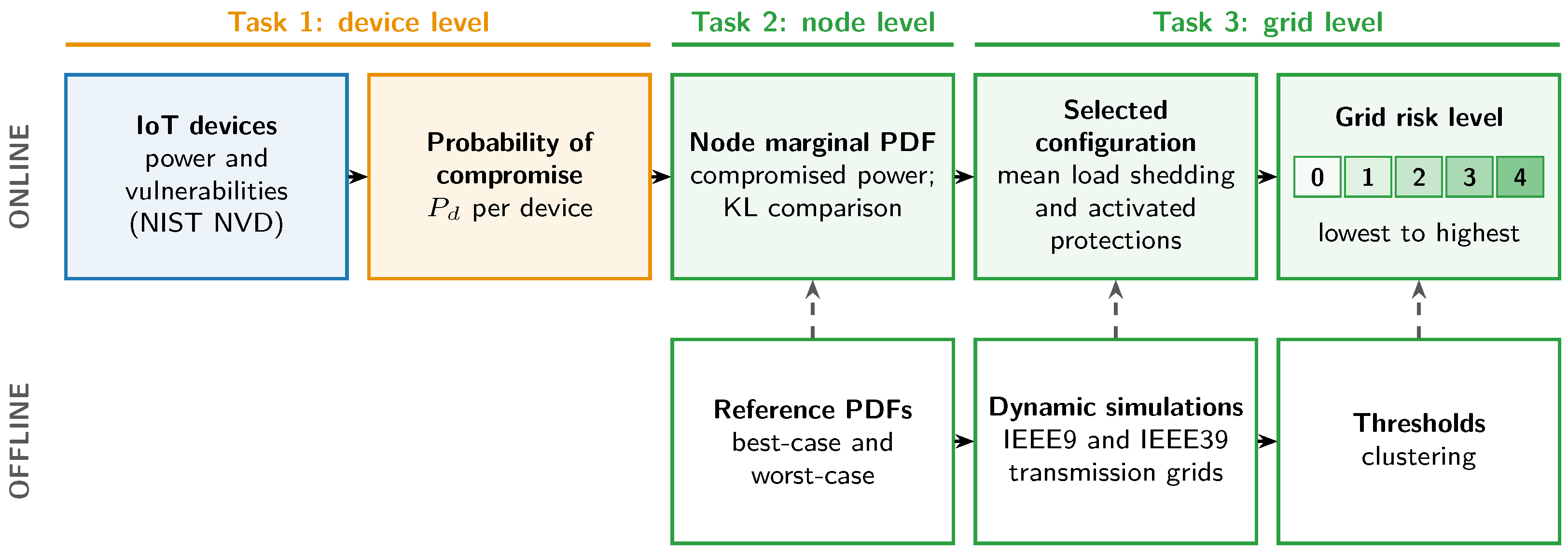
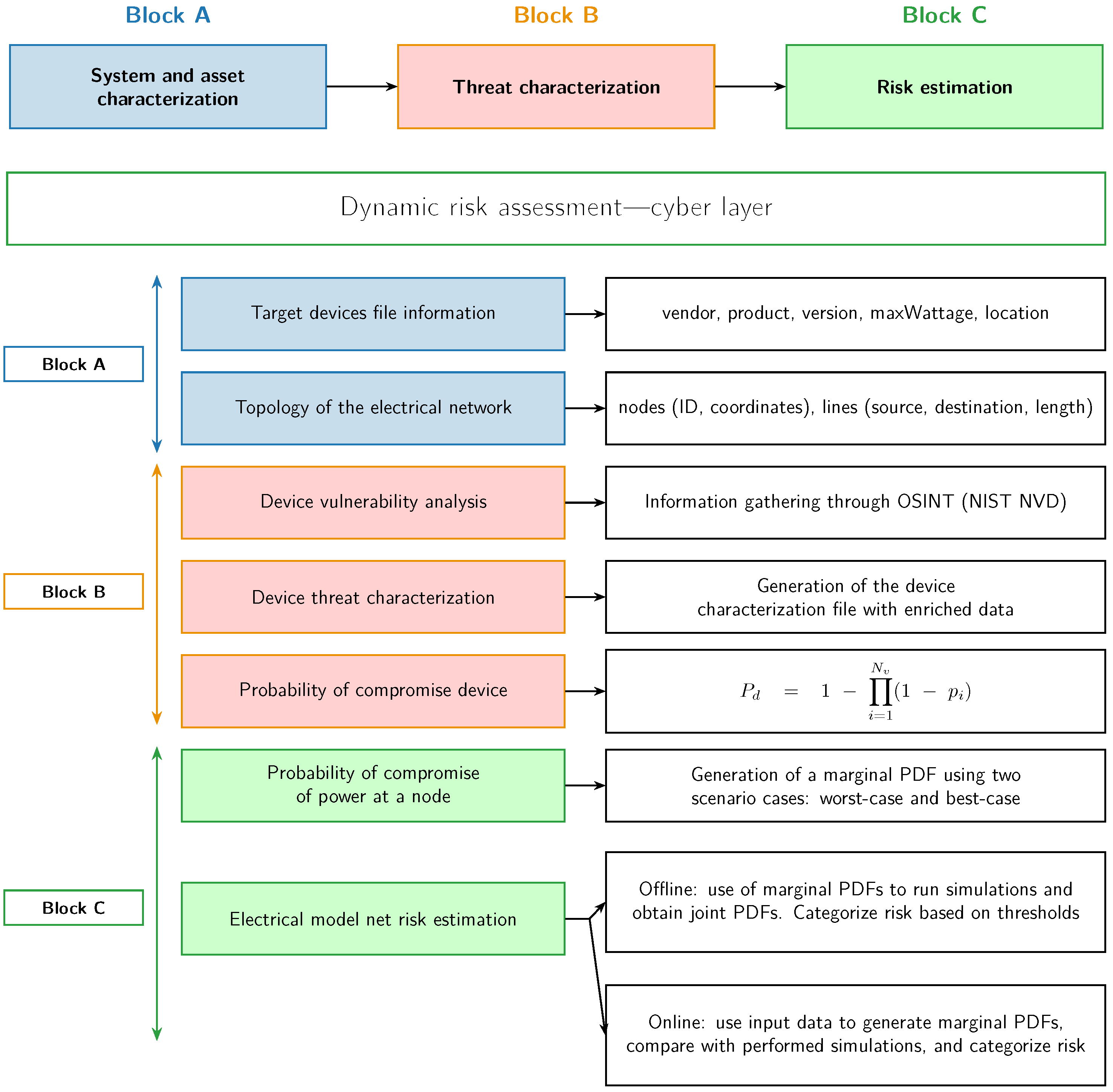
Figure 2. Proposed multilayer architecture for manipulation of demand via Internet of Things (MaDIoT) risk assessment, showing Blocks A (data ingestion), B (vulnerability enrichment), and C (risk estimation with offline/online workflows). Abbreviations: probability density function (PDF), open-source intelligence (OSINT), National Institute of Standards and Technology (NIST), and National Vulnerability Database (NVD).

For the first task, device-level compromise probabilities are assigned by normalizing the vulnerability scores in [14] and aggregating the resulting probabilities, as defined in Section 3. Device characteristics (firmware, version, vendor, etc.) are enriched with open-source intelligence (OSINT) from the National Vulnerability Database (NVD) of the National Institute of Standards and Technology (NIST).

For the second task, the probability of a given compromised power at a node is obtained by generating its marginal probability density function (PDF) through convolution and comparing it with reference PDFs generated via Monte Carlo simulations. Because the device inventories of the load nodes are not publicly available, two extreme scenarios are defined: best-case (few devices with low compromise probability and low power) and worst-case (many devices with high compromise probability and high power), each characterized by three factors: number of devices, compromise probability, and compromised power.

For the third task, grid-level risk estimation is subdivided into offline and online workflows. The offline workflow obtains the joint grid PDF from PowerFactory dynamic simulations under different attack configurations and categorizes it into risk levels using thresholds derived with K-Means++, density-based spatial clustering of applications with noise (DBSCAN), and Gaussian mixture models (GMMs). The online workflow updates the grid risk level by comparing ingested device and topology data with the offline simulated cases (dashed arrows in Figure 1). It assesses potential attack consequences; it does not detect attacks in progress.

The physical consistency of this risk categorization is checked against the frequency, voltages, load shedding, and activated protections observed in the dynamic simulations of transmission grids.

The main contributions of this study are as follows:

• Development of a multilayer architecture that integrates updated device-level vulnerability data with grid-level operational impacts.
• Introduction of a hybrid offline/online methodology that uses probabilistic and clustering-based threshold approaches to update risk estimates as input data change.
• Provision of interpretable risk levels through thresholds derived by clustering from the simulated load shedding and activated protections, with each block of the methodology matched to a phase of NIST Special Publication (SP) 800-30 [15] and of the International Organization for Standardization (ISO)/International Electrotechnical Commission (IEC) standard ISO/IEC 27001 [16] (Section 5).

This article extends the architecture and the offline and online workflows of the conference paper [17] with a revised formulation of the device compromise probabilities (Equation (1)), a correspondence with NIST SP 800-30 and ISO/IEC 27001 (Section 5), a physical consistency check of the risk levels (Section 4.2), quantitative measures to compare the clustering methods (Section 3.4), and tests of the online workflow (Section 3.7).

The remainder of this paper is organized as follows: Section 2 reviews the state of the art and related work. Section 3 describes the proposed multilayer methodology and its offline and online workflows. Section 4 presents the simulation results, including a physical consistency check of the proposed categorization against the simulated system behavior, and compares the K-Means++, DBSCAN, and GMM thresholds. Section 5 discusses the positioning of the proposed approach within the literature, acknowledges the limitations of this work, and outlines future research directions. Finally, Section 6 concludes the paper by summarizing the key findings.

2. State of the Art

Risk analysis is the process of estimating the magnitude of risks faced by an organization or entity. The classical approach to risk analysis typically uses well-defined terms (asset, threat, vulnerability, impact, probability, risk, etc.) and phases (scope definition, asset identification, asset evaluation, threat identification, threat evaluation, and risk assessment).

NIST SP 800-30 provides guidance for conducting risk assessments [15], while ISO/IEC 27001 specifies requirements for establishing and continually improving information security management systems [16]. Dynamic risk assessment (DRA) aims to update risk estimates as vulnerability, monitoring, and system information changes. In parallel, a survey of power grid defense reviews moving target defense across the physical, communication, and control layers [18].

The approaches addressing dynamic risk assessment can be classified according to the data sources used, the model employed, and the type of assessment. The primary data sources include:

• Security Systems: Intrusion detection systems (IDSs), intrusion prevention systems (IPSs), and security information and event management (SIEM) provide alerts and measurements for risk assessment. Cam combines vulnerability information and sensor observations in a Bayesian–Markov model [19]. Awan et al. derive a risk metric from real-time traffic logs [20], while Lin et al. integrate intrusion detection, risk assessment, and adaptive defense selection [21].
• Historical Data: Public databases such as the NIST NVD provide information about known vulnerabilities. Debnath and Xie combine Common Vulnerability Scoring System (CVSS) data with attack graphs for high-performance computing networks [22]. Huang et al. learn Bayesian model parameters from historical data and update them with online observations [23], while Qin et al. use historical attack records and process data to construct an association-based risk model [24].
• System Knowledge Data: Network structure and functional dependencies provide context for risk assessment. Cam and Mouallem relate asset security to mission assurance [25]. Kotenko and Doynikova use attack graphs and service dependencies [26], and Zhu et al. combine a production-process flow model with Bayesian analysis of attack propagation [27]. Other approaches represent time-dependent vulnerabilities in attack graphs [28] or risk propagation among assets [29].
• Expert Opinion: Fu et al. combine expert-defined indices and weights with external data for cyber-physical risk evaluation, using blockchain to support data authenticity [30].

The models can be grouped by their main formulation, although some combine several approaches.

Probabilistic and Data-Driven Models: Zhang et al. use Bayesian networks to represent attack propagation and consequences in industrial control systems [31,32]. Related approaches learn Bayesian parameters from historical data and online observations [23], combine CVSS with attack graphs [22], or infer incident probabilities through association networks [24].

Analytical Models: Dynamic formulations include Bayesian–Markov models [19], non-homogeneous Markov models [28], game-theoretic probabilistic risk assessment for nuclear plants [33], and fuzzy fractional differential equations [34]. Cyber-physical power-system models also combine Supervisory Control and Data Acquisition (SCADA) vulnerabilities with load-shedding consequences [35].

Hybrid Models: Some approaches combine production-process representations with probabilistic attack models [27]. Others link risk assessment to resource-constrained defense selection [36], or integrate cyber and privacy risk assessment with recommendations for safeguards, as in the Automated Cyber and Privacy Risk Management Toolkit [37].

Risk assessment of SCADA systems has been reviewed across critical infrastructures [38]. Bayesian approaches have combined multiple attack scenarios with optimization of security measures for power grids [39], and recent frameworks have extended risk assessment to distribution grids with grid-edge distributed energy resources [40]. Gaussian mixture models have been used to detect false data injection and assess sensor reliability [41]. Quantitative risk assessments may require interpretation and explanation, whereas qualitative scales may give different results across experts unless each level is clearly defined [15]. In the present work, GMM-based classification is applied to the consequences of demand manipulation obtained from power-system dynamic simulations, so that each risk level is defined by thresholds on these consequences.

Our work addresses the less-explored scenario of indirect grid availability failures caused by MaDIoT attacks, in which adversaries exploit IoT device vulnerabilities rather than directly targeting grid systems. In line with cyber-physical energy systems security literature [42], we propose a novel hybrid (quantitative and qualitative) multilayered approach, linking IoT device vulnerabilities with grid-level operational consequences and providing interpretable risk estimations based on thresholds, whose physical consistency is checked against dynamic simulations of the power system under study.

3. Methodology

The proposed model for online risk assessment is part of a broader multilayer architecture that estimates the risk to power grids as cyber-physical systems; this study focuses on the cyber-situational layer.

The architecture of the proposed model (Figure 2) has three high-level blocks (A, B, and C). The blocks are part of the same data flow, but each performs its own tasks:

• Block A: Subprocess responsible for ingesting files containing device characteristics (type, product, brand, version, geolocation, Common Platform Enumeration (CPE) identifiers, and maximum power) and network topology information (in this study, that of the IEEE9 and IEEE39 transmission grids). These input files were generated in a structured JavaScript Object Notation (JSON) format: the device file specifies attributes such as commercial name, type, vendor, version, maximum power, CPE identifier, and geolocation; the network topology file defines nodes (with identifiers and coordinates) and lines (with source, destination, and length).
• Block B: This subprocess enriches the device files from Block A with vulnerability information from the NIST NVD. The multiplicative vulnerability score in [14] is normalized here to assign a Bernoulli parameter $p_i$ to each Common Vulnerabilities and Exposures (CVE) entry. A round considers one exploitation opportunity per CVE:

  $$\begin{array}{cc}\hfill p_i& ={\displaystyle \frac{B_i}{10}}{\displaystyle \frac{E_i}{E_{\max }\left(v_i\right)}}{\omega }_i,\hfill \\ \hfill P_d& =1-{\displaystyle \prod _{i=1}^{N_v}}(1-p_i).\hfill \end{array}$$

  (1)

  Here, $P_d$ is the compromise probability assigned to device d for one round, and $N_v$ is the number of distinct CVEs applicable to device d. For the selected CVSS record, $B_i$, $E_i$, and $v_i$ denote its base score, exploitability score, and version. The reported maxima are $E_{\max }=10.0$ (v2.0) and $3.9$ (v3.0/v3.1) [43,44,45]. The additional attack-vector weights from [14] are ${\omega }_i=1,0.25,0.10,0$ for Network, Adjacent, Local, and Physical, respectively.
  Assuming independent exploitation outcomes under fixed scenario conditions and without exploit chaining, $P_d$ is the complement of the probability that all opportunities fail.
• Block C: Subprocess dedicated to determining and categorizing the overall risk of the power grid. This block is further divided into two consecutive tasks:

  −

  Estimation of the probability of power compromise at a specific node.

  −

  Estimation of the grid-level risk.

To separate preliminary calculations from subsequent risk updates, Block C subtasks were split into two workflows: offline (Section 3.1, Section 3.2, Section 3.3, Section 3.4 and Section 3.5) and online (Section 3.6 and Section 3.7).

The offline workflow (Algorithm S1 in the Supplementary Materials) conducts all preliminary calculations required to establish an empirical basis for the risk classification. These calculations involve the following:

• Generation of reference PDFs for the two extreme scenarios (best-case and worst-case).
• Use of these reference PDFs in dynamic simulations of MaDIoT attacks in PowerFactory to assess the resulting impact on the grid in terms of load shedding and activated protections (underfrequency, overfrequency, undervoltage, and overvoltage). The results form the joint grid PDF.
• Use of the joint grid PDF to calculate thresholds for each characteristic (load shedding and activated protections).
• Estimation of the grid risk level (scalar, bounded) from these thresholds.

The online workflow updates the grid risk level from newly ingested data using the offline simulation results and thresholds, without running new PowerFactory simulations. This workflow includes:

• Calculation of node marginal PDFs from the device compromise probabilities in the enriched file produced by Block B.
• Comparison of each node marginal PDF with the reference PDFs of the best-case and worst-case scenarios.
• Selection, based on marginal PDF comparisons, of the corresponding scenario (best-case or worst-case) for each node and of the resulting grid configuration.
• Acquisition of thresholds associated with the joint grid PDF, which is calculated offline.
• Determination of the grid risk level.

3.1. Offline: Generation of Marginal PDFs for Node Scenario Cases

Device inventories at each node are not publicly available. Two extreme scenarios, best-case and worst-case, were therefore generated to model nodes and serve as offline references. The objective of these scenarios was to create two distinct attack contexts for the grid: one scenario representing a low threat (few devices with a low compromise probability and low power) and another representing a significant threat (many devices with a high compromise probability and high power). When representative node inventories are available, they can guide refinement of the ranges of device numbers in these scenarios. The assigned compromise probabilities can be assessed against the observed outcomes of devices over comparable attack rounds, including rounds without compromise.

To configure these scenarios, a random variable characterized by three distributions was defined as follows:

Number of devices per synthetic node scenario: Modeled by a uniform distribution $U(a,b)$ whose limits depend on the scenario; the two ranges meet at 100 devices, and each spans a factor of 20 between its limits:

• Best-case: $[5,100]$ devices.
• Worst-case: $[100,2000]$ devices.

Device compromise probability: Modeled by a Bernoulli distribution $B\left(p\right)$, where p follows a uniform distribution $U(a,b)$:

• Best-case: $U(0.0,0.3)$
• Worst-case: $U(0.7,1.0)$

These probability ranges match the CVSS scale used in Equation (1). A CVE that is not exploitable over the network gives $p_i\le 0.25$, within the best-case range. A network CVE with maximum exploitability gives $p_i=B_i/10$, so the worst-case range starts at the CVSS High severity threshold of 7.0 [43,44,45]. These ranges set the compromise probabilities of the two reference scenarios, whose grid response is simulated offline (Section 3.3). In the online workflow, the probabilities $P_d$ that Block B assigns from the CVSS records (Equation (1)) replace these probabilities. With the device powers, they determine each node marginal PDF and the most similar scenario for that node. These scenarios select the simulated configuration whose average impact sets the grid risk level (Section 3.6 and Section 3.7).

Compromised device power: Modeled by a uniform distribution $U(a,b)$ with ranges consistent with reported powers of high-wattage household appliances and EV chargers:

• Best-case: $U(0.001,0.003)$ MW (e.g., air conditioners at 1 kW and space heaters at 1.5 kW [2], up to the 3 kW per bot assumed in MaDIoT 2.0 [8]).
• Worst-case: $U(0.003,0.015)$ MW (e.g., electric ovens at 4 kW and electric water heaters at 5 kW [2], and Level 2 EV charging, with a scenario limit of 15 kW within the reported 3.1–19.2 kW range [46]).

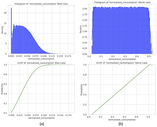
For each scenario, Monte Carlo simulations of this random variable were performed to calculate the PDF and then the empirical cumulative distribution function (ECDF), as shown in Figure 3. The two reference PDFs overlap in compromised power, and each node is matched by its whole PDF (Section 3.7), so its devices need not fall within the ranges of a single scenario. Each scenario involved 1,000,000 Monte Carlo iterations. Each sample of total compromised power was divided by the largest power that the scenario allows, the maximum number of devices times the maximum device power: 0.3 MW for the best case and 30 MW for the worst case. The normalized samples were grouped into 1000 equal bins between 0 and 1, with probabilities that summed to one. The two reference PDFs were generated once and scaled to each node (Section 3.2), so adding grid nodes requires no further Monte Carlo sampling. Generating the samples and the resulting PDF and ECDF took less than 1.5 min per scenario on an Apple M-series laptop with 24 GB of random access memory (RAM). Monte Carlo simulation was used to propagate variability in device counts, compromise probabilities, and power ratings. The joint grid PDF depends on non-linear effects, such as underfrequency load shedding and the operation of generator frequency and load voltage protections, so dynamic simulation is required to determine attack impacts. Monte Carlo simulation is also used in dynamic probabilistic risk assessment of grid cybersecurity to represent interacting system events [47]. For attacks on $N-1$ secure grids, dedicated rare-event sampling can identify damaging load perturbations that ordinary sampling may miss [48].

Figure 3. (a) Normalized probability density function (PDF) and empirical cumulative distribution function (ECDF) for the best-case scenario; (b) normalized PDF and ECDF for the worst-case scenario.

3.2. Offline: Scaling of Node Marginal PDFs

In a power grid model, each node has a maximum power, $P_{\max }$. The two normalized reference PDFs generated in Section 3.1 are scaled by each node’s $P_{\max }$ to obtain the distributions of compromised power used in the grid simulations. A normalized value u thus corresponds to a compromised power of $u{P}_{\max }$ at the node. This scaling ensures that the compromised power in the simulations does not exceed the node’s maximum power. Within each scenario, all nodes share the shape of the reference PDF, and $P_{\max }$ sets the power scale at each node. The scaling preserves the probability of each corresponding power interval. Since device power ratings vary, attack magnitude is expressed as aggregate compromised power in MW at each node. The dynamic simulations in Section 3.3 determine the non-linear grid response to this compromised power.

3.3. Offline: Generation of the Joint Grid PDF

Following the node characterization in Section 3.1 and Section 3.2, this subtask generates the joint grid PDF to characterize the grid and estimate its risk.

The analysis requires grid models. These models are not available to every agent of the power system, but they are available to wholesale market participants and transmission and distribution system operators. For this study, the IEEE9 and IEEE39 transmission grids were selected because their model data are complete, they represent realistic systems (IEEE39 is a version of the New England system), and other studies can reproduce them. The results can be generalized, within limits, to grids with a comparable dynamic response to demand changes, that is, with similar inertia and frequency reserves, load-shedding and protection schemes, and distribution of demand among load nodes. Grid size is not among these conditions. The two grids differ widely in size, yet they give equal or adjacent risk levels for similar fractions of attacked nodes (Section 4). An accurate assessment of a specific power system requires its own grid model and parameters. The two grids represent demand through 3 and 19 aggregated load nodes, respectively. Each load node stands for the distribution grid behind its connection point to the transmission grid. A single distribution feeder has fewer devices than this aggregate. The system frequency responds to the net change in active power demand summed over all attacked nodes, and this study estimates the risk to the grid as a whole, not the impact of each device. Demand is therefore modeled at this aggregated level. This level also avoids modeling the dynamic behavior of the many devices behind each node, which would be very difficult.

Using PowerFactory 2024 SP4 (DIgSILENT GmbH, Gomaringen, Germany), dynamic simulations of MaDIoT attacks were conducted on a university server for each grid model and node scenario type to generate the joint grid PDF. Each simulation was a root mean square (RMS) simulation of 30 s in which the compromised power of each attacked node was applied as a step increase in its active and reactive demand. Load nodes had underfrequency load shedding and voltage relays, and generators had frequency relays (Table S1 in the Supplementary Materials gives the simulation and protection settings). The server had two Intel Xeon Silver 4116 processors, each with 12 cores, and 128 GB of RAM. Each of the 65 configurations below (9 for IEEE9 and 56 for IEEE39) was simulated 1000 times, 65,000 simulations in all. Time per simulation grows with grid size: estimated from the timestamps of the result files, the average was about 2–6 s for IEEE9 and 7–12 s for IEEE39. The online workflow reuses these results for the simulated grids and configurations and runs no new PowerFactory simulations (Section 3.7). On the laptop of Section 3.1, the online workflow computed the node marginal PDFs and compared them with the reference PDFs for the whole IEEE39 grid with 2000 devices in 0.35 s, without the NVD queries.

Data processing and analysis were implemented in Python 3.12.4 using NumPy 2.0.2, pandas 2.2.2, and SciPy 1.13.1; K-Means++, DBSCAN, and GMM were implemented with scikit-learn 1.5.1. The analyses were developed as Jupyter notebooks in Visual Studio Code 1.90, with Matplotlib 3.9.1 and seaborn 0.13.2 used for visualization. Simulation datasets are publicly available in Zenodo (see Data Availability); simulation code is not publicly available.

IEEE9 (3 load nodes):

• Best-case: 1000 simulations per configuration, i.e., for scenarios with 1, 2, and 3 attacked nodes (notation: 1b, 2b, and 3b).
• Worst-case: 1000 simulations per configuration, i.e., for scenarios with 1, 2, and 3 attacked nodes (notation: 1w, 2w, and 3w).
• Mix-case: 1000 simulations per configuration for scenarios involving 2 nodes (1w1b) and 3 nodes (2w1b, 1w2b).

IEEE39 (19 load nodes):

• Best-case: 1000 simulations per configuration, i.e., for scenarios involving 1, 2, …, 19 attacked nodes (notation: 1b, 2b, …, 19b).
• Worst-case: 1000 simulations per configuration, i.e., for scenarios involving 1, 2, …, 19 attacked nodes (notation: 1w, 2w, …, 19w).
• Mix-case: 1000 simulations per configuration, with all 19 load nodes attacked (18w1b, 17w2b, …, 1w18b).

For each simulation, the required number of load nodes was sampled uniformly without replacement from the 3 load nodes of IEEE9 or the 19 of IEEE39. In mix-case configurations, the required numbers of best-case and worst-case scenarios were assigned to these randomly ordered nodes. Simulation results provide data regarding compromised power (active and reactive), demand (initial and final), load shedding, and activated protections (underfrequency, overfrequency, undervoltage, and overvoltage). Load shedding and activated protections were used to generate the joint grid PDF, as these values can vary across nodes depending on their criticality within the grid.

3.4. Offline: Calculation of Thresholds for Selected Characteristics

Thresholds must be defined to delimit the value ranges of each selected characteristic in the joint grid PDF obtained in Section 3.3. These value ranges were subsequently associated with risk levels.

To establish the most suitable thresholds, three clustering algorithms (K-Means++, GMM, and DBSCAN) were applied to the load shedding and activated protections (of any type) and compared.

Load shedding was expressed as a fraction of the initial total demand, and activated protections as a fraction of the relays of each type. The same clustering parameters were used for IEEE9 and IEEE39. K-Means++ used five clusters with k-means++ initialization and random_state=42. GMM used five components with k-means++ initialization, full covariance matrices, and random_state=42. DBSCAN used eps=0.05 and min_samples=12. Five clusters yield the five risk levels defined in Section 3.5, from 0 to 4, consistent with the scales of five levels in NIST SP 800-30 [15]. Five is also the largest number of clusters that keeps the thresholds of every varying characteristic distinct in both grids, and the smallest with which the GMM assigns separate levels to the load shedding of the three 19-node IEEE39 attacks in Section 4.2. The Bayesian information criterion (BIC) gives little guidance on this number, as it improves by only 0.1% from five to ten components in IEEE39. The GMM depends little on the seed: with 30 seeds other than 42, it changed the level of 1.3% of the IEEE39 simulations on average, against 8.6% for K-Means++, and no simulation by more than one level. In IEEE39, the GMM levels also stayed the same with kmeans initialization and with the best of ten initializations, whereas a random initialization reached a lower likelihood and raised the level of 26.0% of the simulations by one. DBSCAN needs no seed, because its result is fixed for given data and parameters.

Each algorithm was fitted jointly to the selected characteristics, and each cluster $i=1,\dots ,K$ was represented by a center with component $c_{i,j}$ for characteristic j: the centroid for K-Means++, the mean for GMM, and the medoid for DBSCAN, whose noise points form no cluster. For each characteristic j, the components of the K centers were sorted as $c_{\left(1\right),j}\le \dots \le c_{\left(K\right),j}$, and the thresholds were set at the midpoints between consecutive values:

$${\tau }_{k,j}={\displaystyle \frac{c_{\left(k\right),j}+c_{(k+1),j}}{2}},k=1,\dots ,K-1.$$

(2)

Table S2 in the Supplementary Materials lists the GMM thresholds.

3.5. Offline: Estimation of Grid-Level Risk Based on Thresholds

The grid risk is determined by the values of the selected characteristics obtained from the simulations in Section 3.3: load shedding and activated protections (of any type). These values are mapped to risk levels using the thresholds defined in Section 3.4. The process is as follows:

• The $K-1$ thresholds ${\tau }_{k,j}$ in Equation (2) divide the values of each characteristic into K consecutive ranges.
• These ranges are associated with risk levels $0,\dots ,K-1$, ordered from the lowest to the highest risk.
• Each simulation from Section 3.3, or each event originating from the online workflow (Section 3.7), yields one value $x_j$ per characteristic, which is compared with the thresholds of the relevant grid model.
• Each value is assigned the risk level of its range, that is, the number of thresholds that it strictly exceeds

  $$r_j={\displaystyle \sum _{k=1}^{K-1}}\mathbf{1}\{x_j>{\tau }_{k,j}\},j=1,\dots ,J,$$

  (3)

  where J is the number of characteristics and $\mathbf{1}\{·\}$ is the indicator function. These levels form the Risk Vector $\overrightarrow{R}=(r_1,\dots ,r_J)$.
• The final grid risk level is the maximum value of the Risk Vector, $R=\max (\overrightarrow{R})$. Each characteristic records a different consequence of the attack, so the most severe one sets the grid risk level, in line with the assessment of maximum impact in NIST SP 800-30 [15]. An average of these levels would let characteristics without impact lower the level of a severe event.

3.6. Online: Generation of Node Marginal PDFs

In the online workflow (Algorithm S2 in the Supplementary Materials), Block A ingests the device inventory and the network topology, and Block B enriches the device records and assigns each device a compromise probability $P_d$ using Equation (1). From these inputs, the workflow derives the node marginal PDFs and compares them with the offline references (Section 3.7).

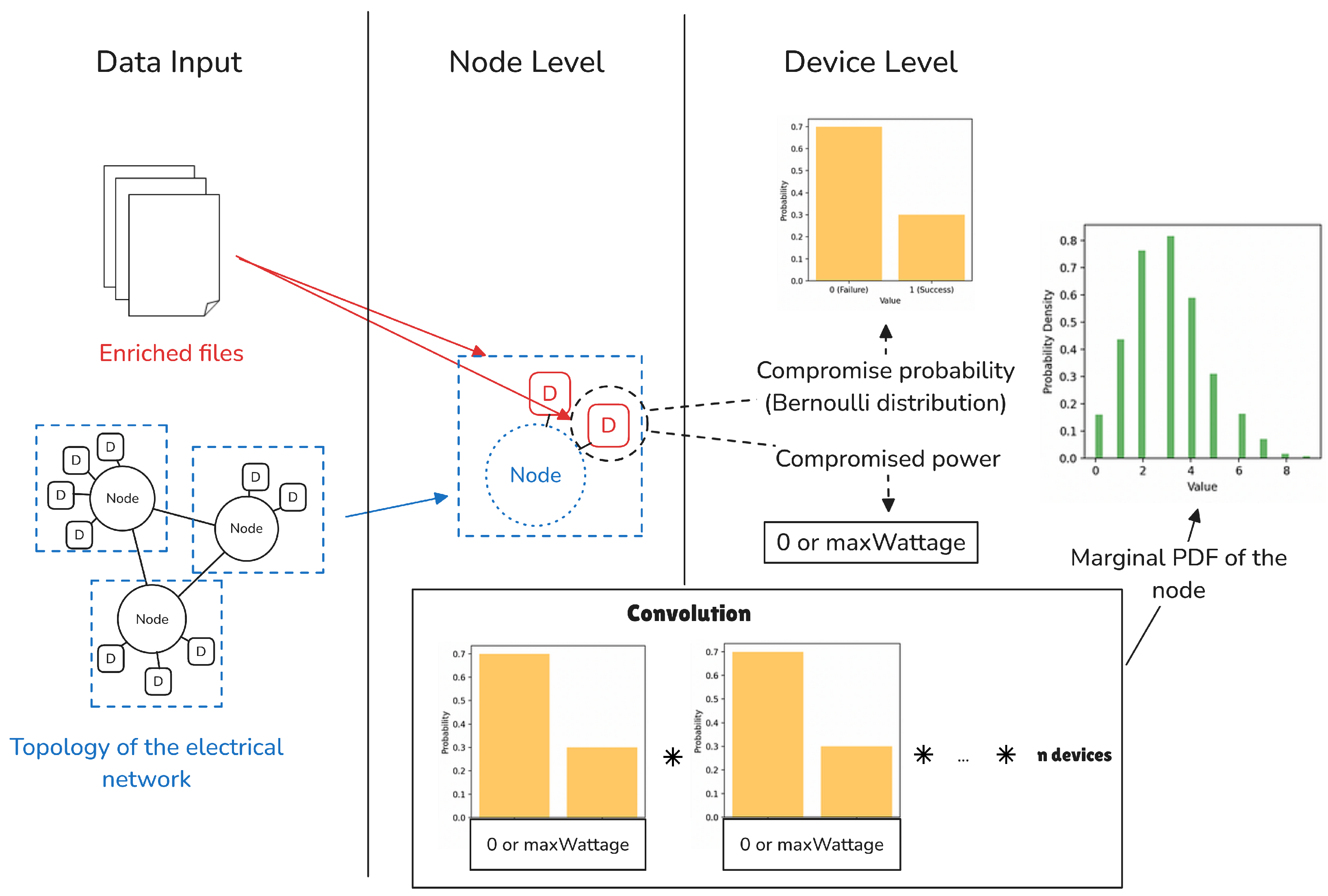
For independent device outcomes, the distribution of their total compromised power is obtained by convolving the individual distributions [49]. Node marginal PDFs were calculated on a grid of 0.1 kW by fast Fourier transform (FFT) convolution, either directly or in its overlap-add form, which gives the same result. The calculation process involved the following:

• Successful compromise is assumed to allow demand manipulation. For each device d, the compromised power $X_d$ takes the value $P_{\max ,d}$ with probability $P_d$ (Equation (1)) and 0 otherwise.
• The total compromised power at a node with D devices is $S={\sum }_{d=1}^D{X}_d$. Under a separate assumption of independence among devices, the PDF of S is obtained by convolving the individual PDFs. This convolution is computed efficiently by applying the FFT to each individual PDF, multiplying the results element-wise in the frequency domain, and applying the inverse FFT:

  $$f_S={\mathcal{F}}^{-1}\left({\displaystyle \prod _{d=1}^D}\mathcal{F}\left(f_{X_d}\right)\right)$$

  (4)

  where $\mathcal{F}$ denotes the FFT and $f_{X_d}$ is the PDF of device d. The outcome is the node marginal PDF. Each $P_{\max ,d}$ was rounded to the nearest 0.1 kW, the transforms were padded to give a linear convolution, and small negative values from floating-point arithmetic were set to zero before the PDF was rescaled to unit sum.

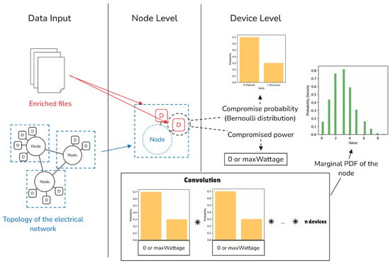
This procedure was applied to each node of the grid, as illustrated in Figure 4.

Figure 4. Online workflow for node marginal probability density function (PDF) generation using fast Fourier transform (FFT) convolution. Boxes labeled D represent devices, arrows show the flow of data, and ∗ denotes convolution.

3.7. Online: Grid-Level Risk Estimation

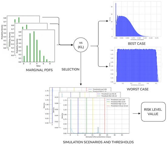
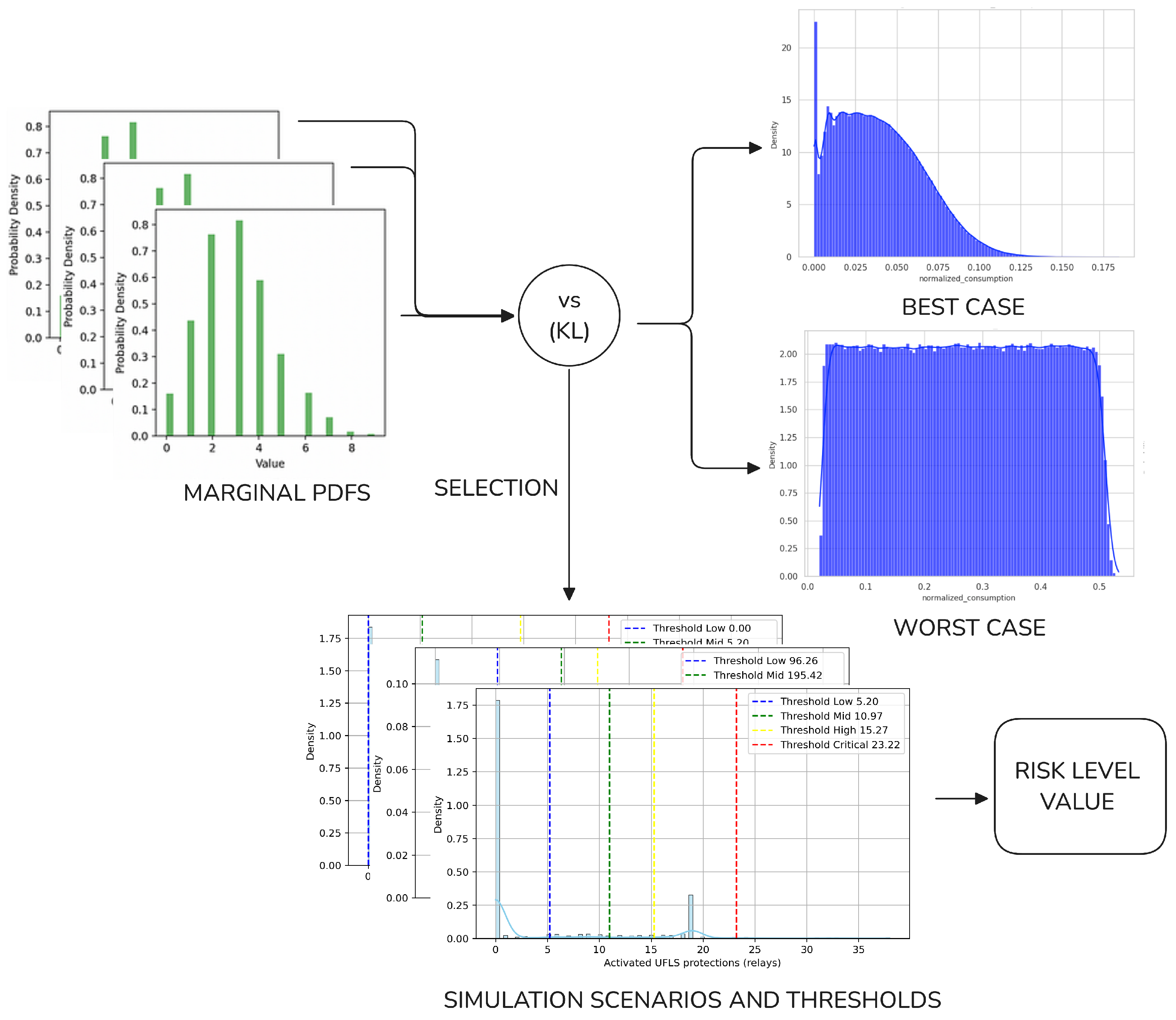
Using the node marginal PDFs obtained in Section 3.6, the online workflow estimates grid-level risk as follows (see Figure 5):

Figure 5. Online grid-level risk estimation process using Kullback–Leibler (KL) divergence comparison and threshold-based categorization. The lower plots show the GMM thresholds of the IEEE39 grid for undervoltage protections, load shedding, and underfrequency protections. Abbreviations: probability density function (PDF) and underfrequency load shedding (UFLS). The overlapping plots on the left represent the marginal PDFs of several nodes.

• Each node marginal PDF was compared with the reference PDFs of the two offline scenarios (Section 3.1 and Section 3.2) using the Kullback–Leibler (KL) divergence, and the most similar scenario was selected. This comparison was performed for each node. For this comparison, the power values of the node PDF were divided by the node’s $P_{\max }$ and accumulated in the 1000 bins of the reference PDFs (Section 3.1), with any mass above $P_{\max }$ in the last bin. With $a_i$ and $q_i$ the probabilities of bin i in the node PDF and in a reference PDF, the divergence was $D_{\mathrm{KL}}={\sum }_{a_i>0}{a}_i\ln (a_i/{\tilde{q}}_i)$, where ${\tilde{q}}_i=(q_i+{10}^{-12})/{\sum }_j(q_j+{10}^{-12})$. Empty reference bins therefore add a large but finite term. The KL divergence is a common measure for comparing probability distributions, and the selected scenario depends little on this choice. Five test inventories distribute 10, 100, 200, 1000, and 2000 devices of up to 15 kW over the 19 load nodes of the IEEE39 grid. With the Wasserstein distance, the same scenario was selected for 80 of their 81 nodes with devices (98.8%). The one node that differed lay where the two scenario PDFs overlap. There, the KL divergence selected the worst case, because it strongly penalizes power values that are likely for the node but unlikely in the best case, and the risk level rose by one. The KL divergence is therefore the conservative choice. Some nodes fall outside both reference PDFs. A node whose mean compromised power was below the smallest nonzero value of the best case was assigned to the best case, and a node whose mean was above the largest value of the worst case was assigned to the worst case. For a node between the two references, choosing the worst case instead of the best case increases the number of worst-case nodes by one. In the simulated configurations of the IEEE39 grid, moving one node from the best case to the worst case never reduced the average load shedding or activated protections, and the risk level of these averages stayed the same or rose by one level.
• Once the most similar scenario for each node was identified, all simulations of the resulting configuration (Section 3.3) were retrieved, and their values were averaged.
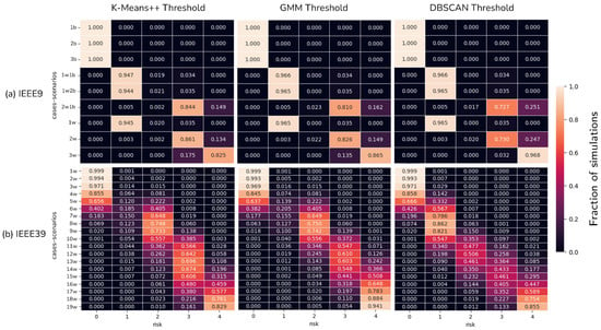
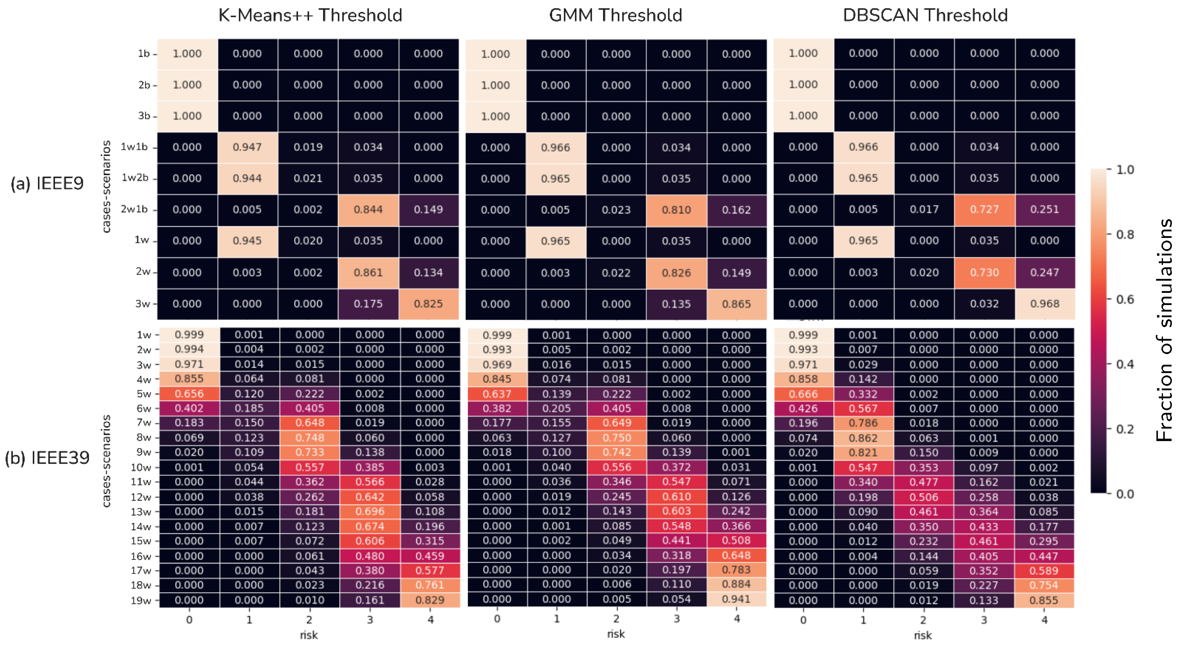
• The average values were then placed in the ranges defined by the thresholds of Section 3.4. The rows of Figure 6 show how the simulations of each configuration are spread over the risk levels, including those above the level of the average.
  

  Figure 6. Heat maps showing risk level assignments for K-Means++, density-based spatial clustering of applications with noise (DBSCAN), and Gaussian mixture models (GMMs): (a) IEEE9 grid with best-case, worst-case, and mix-case scenarios; (b) IEEE39 grid worst-case scenarios only. The Y-axis (cases-scenarios) denotes the attack configuration, where the number indicates the count of attacked nodes and the suffix indicates the scenario type (b = best-case, w = worst-case).
• The corresponding risk level was assigned using the mapping established in Section 3.5.

In the test inventory of step 1 with 1000 devices of ten commercial products, Equation (1) assigns $P_d$ from 0.83 to 1 to the 700 devices whose products have CVEs exploitable over the network in the NVD. At the load node with $P_{\max }=4.6$ MW, 240 devices give a node marginal PDF with a mean of 0.28 $P_{\max }$, which the KL divergence matches to the worst case, and the other 18 nodes take the best case. None of the 1000 simulations of this configuration show load shedding or protection activation, so the grid risk level is 0. Scaling all $p_i$ by 0.5 or 1.5, with a maximum of 1, changed no selected scenario.

The node marginal PDFs assume independent devices (Section 3.6). Devices of the same product, however, share firmware and vulnerabilities, so one exploit may compromise many of them at once. This dependence keeps the expected compromised power of a node but widens its PDF, and a wider PDF may match a different scenario in step 1. To measure this effect, the five inventories of step 1 were evaluated again with a one-factor Gaussian copula: a common random factor couples the compromise of devices of the same product, or of all devices at a node, while each device keeps its $P_d$. In this test, all devices received the same $P_d$, 0.15, 0.5, or 0.85, and the correlation took illustrative values up to 0.3. No node changed scenario, and the grid risk level did not change. Nodes outside the range of the reference PDFs kept their scenario, because dependence does not change their mean compromised power (step 1).

The offline simulations are run once for each power system and serve all later assessments. Changes in device inventories and vulnerabilities, and ordinary changes in the grid, need no new simulations. The former enter through the online workflow, and the latter do not alter the dynamic response of the grid, on which the results depend (Section 3.3). When a structural change, such as new generators or lines or new connection requirements, alters that response, only the grid simulations and thresholds are repeated with the updated grid model (Section 3.3 and Section 3.4), while the scenario reference PDFs (Section 3.1) and the online workflow remain the same.

4. Results

4.1. Evaluating Clustering Methods Across IEEE9 and IEEE39 Grids

To evaluate the performance of the proposed methodology, the results of grid-level risk estimation were analyzed for the IEEE9 and IEEE39 grid models, considering various attack scenarios.

The heat maps in Figure 6 show the risk level assignments (X-axis) for each case (Y-axis) and each clustering method used for the thresholds of the offline workflow.

The assigned risk levels range from 0 to 4. Level 0 corresponds to scenarios with no load shedding or protection activation; levels 1–2 represent increasing stress with less load shedding and fewer activated protections than levels 3–4; and levels 3–4 capture more severe conditions, including faster frequency drops and disconnection of significant portions of demand through under-frequency protections, as the cases in Section 4.2 show.

Colors and cell values indicate the fraction of simulations assigned to each risk level for a given attack configuration. Each row sums to one, apart from rounding.

Figure 6a shows the risk estimation for different clustering methods on the IEEE9 grid. The observations from these heat maps include the following:

• Best-case scenarios consistently received the lowest risk level, indicating minimal risk contribution from attacks of this nature.
• Mix-case scenarios consistently aligned with their worst-case scenario counterparts across all clustering methods. Because best-case scenarios contribute little to grid risk, the risk arises mainly from nodes simulated under worst-case conditions. Consequently, mix-case scenarios 1w1b and 1w2b closely match worst-case scenario 1w, and mix-case scenario 2w1b resembles worst-case scenario 2w.
• The risk estimation of worst-case scenarios depends on the clustering method. The DBSCAN thresholds gave more dispersed levels (in 2w and 2w1b, 27.0% and 27.3% of its simulations fall outside the most frequent risk level, against 13.9% and 15.6% for K-Means++ and 17.4% and 19.0% for GMM), whereas the K-Means++ and GMM thresholds gave a more progressive estimation (along 1w, 2w, and 3w, the two increases in mean risk level differ by 1.34 levels for K-Means++ and 1.31 for GMM, against 1.40 for DBSCAN).

Figure 6b shows only the worst-case scenarios for the IEEE39 grid, because its best-case and mix-case results were similar to those of IEEE9. These heat maps show that all three clustering methods yield a progressive, diagonal estimation. However, the mean risk level of DBSCAN falls more than half a level below the diagonal from 4w to 9w. Relative to the level of the diagonal for each configuration, rounded to the nearest level, the GMM placed 27.1% of the simulations above and 16.6% below (mean deviation of +0.112 levels), K-Means++ 23.0% and 20.3% (+0.025), and DBSCAN 8.7% and 37.6% (−0.303). The GMM is the most conservative of the three methods in every worst-case configuration of IEEE39. Because underestimation leaves a grid exposed, the methodology favors overestimation within the risk tolerance of each operator [15], through the maximum over the characteristics (Section 3.5) and the KL selection in the overlap of the scenario PDFs (Section 3.7).

All clustering methods were analyzed and compared based on the most descriptive characteristics from the PowerFactory simulations: load shedding and activated protections (underfrequency, overfrequency, undervoltage, and overvoltage).

Table 1 compares the thresholding methods based on the risk distributions in Figure 6. Intra-case variability refers to the spread of risk assignments within the same attack configuration, whereas inter-case dispersion measures how well different attack configurations are separated into distinct risk levels. With the measures of Table 1, the GMM showed the lowest intra-case variability in the worst-case configurations of the IEEE39 grid, where 28.3% of its simulations fall outside the most frequent risk level of their configuration, against 29.5% for K-Means++ and 31.3% for DBSCAN. For inter-case dispersion, only one of these configurations has no risk level with more than half of the GMM simulations, against two for K-Means++ and five for DBSCAN. For progressive estimation, the mean risk levels of the GMM and K-Means++ stay within 0.43 and 0.44 levels of the diagonal of Figure 6b, against 0.63 for DBSCAN. For smooth transitions, the GMM gives the most regular increases in mean risk level along the worst-case configurations of the IEEE9 grid (Table 1). These results, together with the most conservative risk levels and a smaller dependence on the random seed than K-Means++ in the IEEE39 grid (Section 3.4), led to the selection of the GMM for the two grids studied.

Table 1. Comparison of K-Means++, density-based spatial clustering of applications with noise (DBSCAN), and Gaussian mixture models (GMMs).

Property	Measure	K-Means++	DBSCAN	GMM
Progressive estimation	Largest deviation of the mean level from the diagonal (IEEE39)	Yes (0.44)	No (0.63)	Yes (0.43)
Smooth transitions	Difference between the two increases in mean level, 1w–3w (IEEE9)	Moderate (1.34)	Low (1.40)	High (1.31)
Overestimation tendency	Simulations above the rounded diagonal (IEEE39)	Slight (23.0%)	No (8.7%)	Yes (27.1%)
Underestimation tendency	Simulations below the rounded diagonal (IEEE39)	No (20.3%)	Yes (37.6%)	No (16.6%)
Intra-case variability	Simulations outside the most frequent level (IEEE39)	Moderate (29.5%)	High (31.3%)	Low (28.3%)
Inter-case dispersion	Configurations with no level above one half (IEEE39)	Good (2)	Poor (5)	Excellent (1)

To check that the GMM assigns physically consistent risk levels, the transients of one simulated attack of each risk level were studied in both transmission grids. Between neighboring risk levels, the check compares the disconnected demand, the speed of the frequency drop, and the under-frequency load shedding threshold reached (Section 4.2).

4.2. Physical Consistency Check of the GMM Risk Levels

The application of unsupervised machine learning techniques to classify the risk of potential MaDIoT attacks raises the question of whether the assigned risk levels are reasonable and aligned with the impact that a system operator would observe in the network.

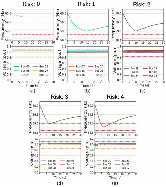
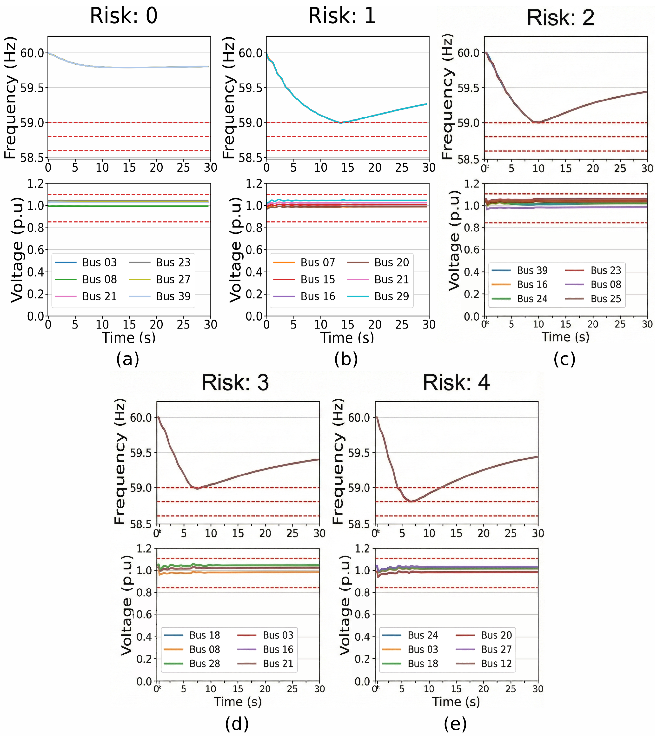
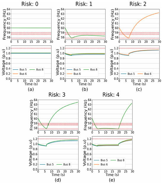
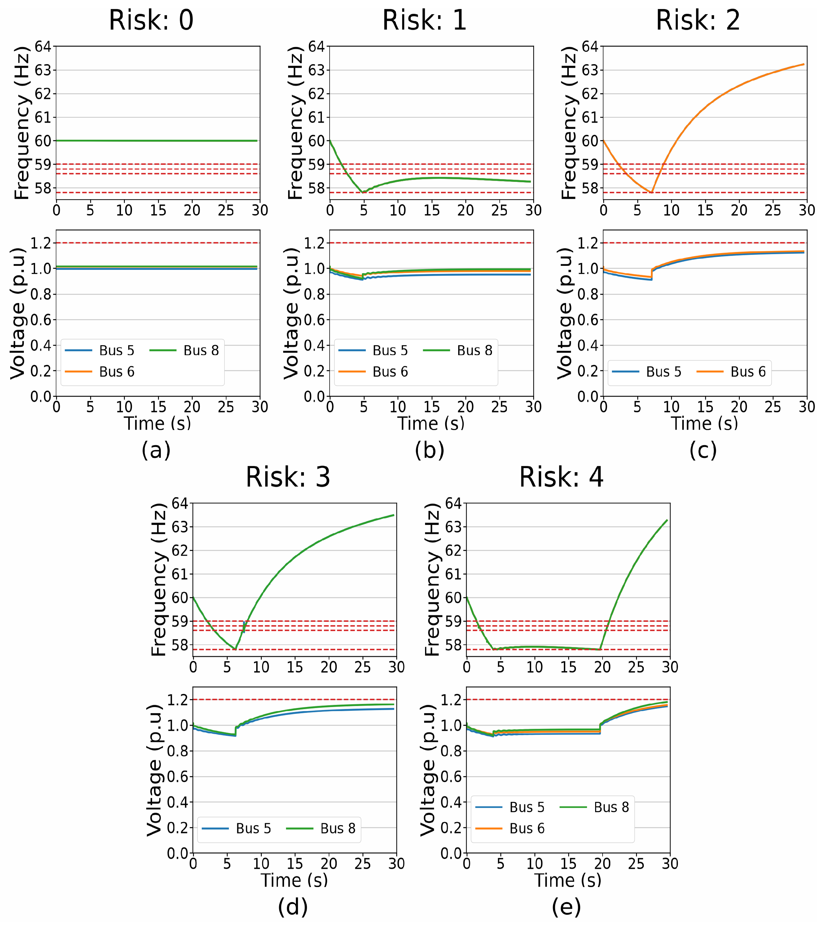
The dynamics of both transmission grids were analyzed for one MaDIoT attack of each risk level, from 0 to 4. In the IEEE39 grid, the attacks of risk levels 2, 3, and 4 are three 19-node attacks (worst case). The risk 0 and 1 attacks in the IEEE39 grid and the five attacks in the IEEE9 grid come from the published simulation datasets (Data Availability Statement) and were simulated again to record their transients. Their disconnected demand and activated protections match the published records. Figure 7 and Figure 8 plot the frequency and voltages of some compromised nodes in the IEEE39 and IEEE9 grids.

Figure 7. Frequency and voltages in the IEEE39 when performing MaDIoT attacks categorized as risk 0 (a), 1 (b), 2 (c), 3 (d), and 4 (e): an attack on 19 nodes (best case) in (a), on 11 nodes (worst case) in (b), and on 19 nodes (worst case) in (c–e). For readability, six of the attacked nodes are shown, labeled by bus; their frequency curves nearly coincide because frequency is almost uniform across the grid. Red-dashed lines indicate the threshold for the activation of protections. Voltages are expressed in per unit (p.u.). The attack is applied at $t=0$ s in all cases.

Figure 8. Frequency and voltages in the IEEE9 when performing MaDIoT attacks categorized as risk 0 (a), 1 (b), 2 (c), 3 (d), and 4 (e): an attack on 3 nodes (best case) in (a), on 2 nodes (worst case) and 1 node (best case) in (b), on 2 nodes (worst case) in (c,d), and on 3 nodes (worst case) in (e). All attacked nodes are shown, labeled by bus; their frequency curves nearly coincide because frequency is almost uniform across the grid. Red-dashed lines indicate the threshold for the activation of protections. Voltages are expressed in per unit (p.u.). The attack is applied at $t=0$ s in all cases.

In the risk 0 attack in Figure 7a, frequency falls slowly to 59.79 Hz and stays above the first under-frequency load shedding threshold (59 Hz), so no demand is disconnected. In the risk 1 attack in (b), frequency falls faster and reaches 59 Hz about 14 s after the attack. The under-frequency protections disconnect 98.98 MW (1.6% of the initial demand), less than half of the 213.88 MW disconnected in the risk 2 attack, which justifies the lower risk level.

Figure 7c,d show, at a high level, similar dynamics for risk 2 and 3 attacks, respectively. However, there are some differences that justify the different risk assignments. Although frequency drops in both cases until the first under-frequency load shedding threshold (59 Hz) due to the lack of inertia in the system, it can be noticed that the MaDIoT attack in (d) causes a faster frequency decrease (i.e., more MW of demand are compromised) than the risk-2 attack, triggering under-frequency protections in the system that disconnect 304.85 MW (5% of the initial demand) compared to the 213.88 MW (3.5%) disconnected in the risk-2 attack. Therefore, although the frequency curves look similar for the risk 2 and 3 attacks, their underlying different impact is correctly processed by the GMM for the risk assignment.

Regarding Figure 7e, where a risk-4 attack is shown, frequency drops until the second frequency threshold (58.8 Hz), disconnecting 540.23 MW (8.9%) through the under-frequency protections; thus the maximum risk level is correctly assigned. This shows that the GMM algorithm is reasonably classifying the risk of MaDIoT attacks; this classification may seem conservative (the maximum risk does not necessarily imply a full blackout of the system), but it should be considered that frequency is critical for system operation and that frequency variations greater than 0.1–0.2 Hz are rare in the daily operation of large power systems.

Figure 8 shows the five risk levels in the IEEE9 grid, with thresholds from the simulations of this grid (Section 3.4). Here the under-frequency protections disconnect demand only at 57.8 Hz, the lowest red line, half the demand of one load node at a time. The risk 0 attack in (a) leaves frequency and voltages flat. In (b)–(e), frequency falls to 57.8 Hz, and the risk level grows with the disconnected demand: one load node in (b) (50 MW, 15.9% of the initial demand), two in (c) and (d) (107.5 and 112.5 MW, 34.1 and 35.7%), and three in (e) (157.5 MW, 50%). In (e), frequency falls fastest and stays at 57.8 Hz for about 16 s, until the other two load nodes are disconnected. The risk 1 attack compromises more demand than the risk 2 attack (94.14 versus 75.50 MW) and its frequency falls faster, but it disconnects one load node instead of two. After load shedding, frequency rises above 60 Hz in (c)–(e), where the disconnected demand exceeds the compromised demand, and stays below 58.5 Hz in (b). As in Figure 6a, attacks on best-case nodes are risk 0, and most attacks on two and three worst-case nodes are risk 3 and 4, as in Figure 8d,e. The attacks in Figure 8b,c are less frequent outcomes of attacks on two worst-case nodes.

In the IEEE39 grid, the plotted voltages show an initial dip and damped oscillations within protection limits, even in the risk-4 case. In the IEEE9 grid, voltages rise after load shedding in the risk 2 to 4 attacks, up to 1.18 p.u., below the overvoltage threshold (1.2 p.u.). Voltage recovery should be interpreted alongside frequency deviations and disconnected demand.

Regarding model stability, Monte Carlo sampling (1,000,000 iterations per scenario and 1000 PowerFactory simulations per configuration) is used to limit sampling variability. With fixed thresholds, small perturbations leave the risk level unchanged unless the assessed indicators cross a threshold. In electrically strong areas, a low risk level reflects limited load shedding and protection activation in the simulated scenarios; frequency and voltage deviations are not scored separately.

5. Discussion

The results presented in Section 4 demonstrate that the proposed methodology produces risk levels that are interpretable and physically consistent with the simulated grid response in the cases examined. This section discusses the positioning of the proposed approach within the broader literature, acknowledges the limitations of this work, and outlines directions for future research.

The proposed approach is positioned within the quantitative/machine-learning stream of dynamic cyber-risk assessment reviewed in Section 2 (e.g., Bayesian/machine-learning and related models fed by IDS/IPS/SIEM, historical vulnerability data, and system-knowledge data) and addresses the gap in research on indirect MaDIoT-driven availability failures with an interpretable, threshold-based categorization. The methodology applies the classical risk analysis described in Section 2, that is, the risk assessment process set out in NIST SP 800-30 [15] and ISO/IEC 27001 [16], and adapts it to MaDIoT attacks. Table 2 shows the block of the methodology that covers each phase. As in these standards, risk combines probability and impact. The adaptation lies in how both are obtained: the vulnerabilities of IoT devices give the probability of each compromised power at each load node, and the dynamic response of the grid gives the impact.

Table 2. Correspondence between the phases of classical risk analysis, the requirements of NIST SP 800-30 and ISO/IEC 27001, and the proposed methodology.

Phase	NIST SP 800-30 [15] and ISO/IEC 27001 [16]	Proposed methodology
Scope definition and asset identification	Purpose, scope, assumptions, and risk model; critical assets in the asset/impact-oriented approach (NIST Tasks 1-1 to 1-5). Risks within the defined scope (ISO 6.1.2 c)	Block A: device inventory and grid topology (Section 3). Availability of the power supply under MaDIoT attacks on load nodes (Section 1)
Asset evaluation (impact)	Adverse impacts on operations and assets (NIST Task 2-5). Potential consequences (ISO 6.1.2 d)	Block C, offline: load shedding and activated protections from dynamic simulations of the compromised power at each node (Section 3.2 and Section 3.3)
Threat identification (threat, vulnerability)	Threat sources and events; vulnerabilities and predisposing conditions (NIST Tasks 2-1 to 2-3). Risk identification (ISO 6.1.2 c)	Coordinated MaDIoT attacks on configurations of load nodes (Section 3.3). Block B: device vulnerabilities from the NIST NVD (Section 3)
Threat evaluation (probability)	Likelihood of initiation and of adverse impact (NIST Task 2-4). Realistic likelihood (ISO 6.1.2 d)	Block B: compromise probability $P_d$ per device and attack round (Equation (1)). Block C: node PDFs of compromised power; offline, by Monte Carlo for two reference scenarios; online, by convolution, matched to a reference by the KL divergence (Section 3.1, Section 3.6 and Section 3.7)
Risk assessment (risk)	Combination of likelihood and impact (NIST Task 2-6). Levels of risk (ISO 6.1.2 d)	Block C: GMM thresholds define five levels (Equation (2)); each simulation receives a level, and $R=\max (\overrightarrow{R})$ (Equation (3)). Online: the level of the mean impact of the matched configuration (Section 3.7)
Risk update	Monitor risk factors and update the assessment (NIST Tasks 4-1 and 4-2). Reassessment at planned intervals or after significant changes (ISO 8.2)	Online workflow: new inventories and vulnerabilities update the level without new simulations; significant grid or regulatory changes require new simulations and thresholds (Section 3.7)

Beyond power grids, Blocks A and B and the threshold categorization could be adapted to other cyber-physical systems with many connected devices, such as low-altitude intelligent networks with integrated sensing and communication [50,51,52]. The adaptation requires that the compromised devices add up to a single magnitude at each node, such as injected traffic, and that a model of that system, with its own severity indicators, replace the dynamic grid simulation.

Nevertheless, this work has several limitations: (1) the model currently relies on two transmission grids (IEEE9 and IEEE39), with the physical consistency of the risk levels checked in dynamic simulations rather than under real operating conditions; further validation across diverse grid models would enhance its general applicability; (2) the compromise probabilities are model-assigned and uncalibrated, and shared preconditions may violate the assumed independence among exploitation opportunities or among devices: within one device, such a common cause places $P_d$ between the largest $p_i$ and the value of Equation (1), which therefore tends to overestimate $P_d$, and among devices, the sensitivity test in Section 3.7 keeps the reference PDFs and thresholds obtained under independence, whose response to dependence requires new dynamic simulations; (3) the current implementation uses two extreme scenarios (best-case and worst-case) to bound uncertainty, providing a conservative risk envelope within the simulated configurations (Section 3.7), but the grid risk levels obtained when nodes lie between the two references have not been checked directly against dynamic simulations of intermediate scenarios, and the change of risk level observed in IEEE39 when one node moves from the best case to the worst case applies to the simulated configurations only; (4) the OSINT-based vulnerability enrichment in Block B depends on public databases such as the NIST NVD, which lack entries for some device models and firmware versions [53], leave recently published vulnerabilities without analysis [54], and miss zero-day exploits or undisclosed vulnerabilities, and which lag behind IoT attack techniques that keep evolving, from botnets of high-wattage appliances [2,8] to attacks on electric vehicle charging [3,4,5,6] and on distributed energy resources [7]; and (5) demand is represented by aggregated loads at transmission nodes, without modeling distribution feeders or the dynamic behavior of individual devices, so local effects in distribution grids, such as voltage drops and the operation of feeder protections, are not reflected in the risk levels.

Future research will address the comparative evaluation of the framework and its integration with SCADA, advanced metering infrastructure, energy management systems, and distributed energy resource management systems. Neither has been performed in this study; the aim is to complement operational monitoring and analysis with vulnerability-based MaDIoT risk estimates. Further work includes modeling dependencies among vulnerabilities [55,56] and among devices that share firmware, together with their effect on the reference PDFs and thresholds, hardware-in-the-loop validation, global sensitivity analysis of model inputs [57], and using risk estimates to guide response selection [58].

6. Conclusions

This paper presents a multilayer methodology for estimating grid-level risk in the IEEE9 and IEEE39 grids under MaDIoT attacks. The methodology is interpretable and consistent with classical risk analysis through its treatment of assets, threats, vulnerabilities, probability, impact, and risk, as detailed in Table 2.

Block A performs system/asset characterization (scope definition and asset identification). Block B enriches device attributes with NIST NVD vulnerability information and assigns compromise probabilities for an attack round through the normalized scoring model adapted from [14]. Block C uses probabilistic methods and clustering-based thresholding to derive bounded risk levels, whose physical consistency was checked against the load shedding and protection activations in the dynamic simulations.

References

- Maleki, S.; Pan, S.; Lakshminarayana, S.; Konstantinou, C. Survey of Load-Altering Attacks Against Power Grids: Attack Impact, Detection, and Mitigation. IEEE Open Access J. Power Energy 2025, 12, 220–234. [Google Scholar] [CrossRef] [Scilit]
- Soltan, S.; Mittal, P.; Poor, H.V. BlackIoT: IoT Botnet of High Wattage Devices Can Disrupt the Power Grid. In Proceedings of the 27th USENIX Security Symposium; USENIX: Berkeley, CA, USA, 2018; pp. 15–32. [Google Scholar]
- Kabir, M.E.; Ghafouri, M.; Moussa, B.; Assi, C. A Two-Stage Protection Method for Detection and Mitigation of Coordinated EVSE Switching Attacks. IEEE Trans. Smart Grid 2021, 12, 4377–4388. [Google Scholar] [CrossRef] [Scilit]
- Acharya, S.; Khan, H.A.U.; Karri, R.; Dvorkin, Y. MaDEVIoT: Cyberattacks on EV Charging Can Disrupt Power Grid Operation. In 2024 IEEE Power & Energy Society Innovative Smart Grid Technologies Conference (ISGT); IEEE: New York, NY, USA, 2024. [Google Scholar]
- Jarauta Gastelu, J.; Gesteira-Miñarro, R.; Matanza, J.; Palacios, R.; López, G. MitM Attack to Electric Vehicle AC Chargers. IEEE Internet Things J. 2025, 12, 39689–39700. [Google Scholar] [CrossRef] [Scilit]
- Elmo, D.; Fragkos, G.; Johnson, J.; Rohde, K.; Salinas, S.; Zhang, J. Disrupting EV Charging Sessions and Gaining Remote Code Execution with DoS, MITM, and Code Injection Exploits using OCPP 1.6. In 2023 Resilience Week (RWS); IEEE: New York, NY, USA, 2023; pp. 1–8. [Google Scholar] [CrossRef] [Scilit]
- Rodríguez-Pérez, N.; Matanza, J.; Sigrist, L.; Rueda Torres, J.; López, G. MaDIoT 3.0: Assessment of Attacks to Distributed Energy Resources and Demand in a Power System. IEEE Open Access J. Power Energy 2025, 12, 552–563. [Google Scholar] [CrossRef] [Scilit]
- Shekari, T.; Cardenas, A.A.; Beyah, R. MaDIoT 2.0: Modern High-Wattage IoT Botnet Attacks and Defenses. In Proceedings of the 31st USENIX Security Symposium; USENIX: Berkeley, CA, USA, 2022; pp. 3539–3556. [Google Scholar]
- Shekari, T.; Irvene, C.; Cardenas, A.A.; Beyah, R. MaMIoT: Manipulation of Energy Market Leveraging High Wattage IoT Botnets. In Proceedings of the 2021 ACM SIGSAC Conference on Computer and Communications Security; ACM: New York, NY, USA, 2021; pp. 1338–1356. [Google Scholar]
- Baggott, S.S.; Santos, J.R. A Risk Analysis Framework for Cyber Security and Critical Infrastructure Protection of the U.S. Electric Power Grid. Risk Anal. 2020, 40, 1744–1761. [Google Scholar] [CrossRef] [Scilit] [PubMed]
- Ospina, J.; Liu, X.; Konstantinou, C.; Dvorkin, Y. On the Feasibility of Load-Changing Attacks in Power Systems During the COVID-19 Pandemic. IEEE Access 2021, 9, 2545–2563. [Google Scholar] [CrossRef] [Scilit] [PubMed]
- Liu, X.; Shahidehpour, M.; Li, Z.; Liu, X.; Cao, Y.; Li, Z. Power System Risk Assessment in Cyber Attacks Considering the Role of Protection Systems. IEEE Trans. Smart Grid 2017, 8, 572–580. [Google Scholar] [CrossRef] [Scilit]
- Rodríguez-Pérez, N.; Matanza Domingo, J.; Sigrist, L.; Rueda Torres, J.L.; López López, G. Confronting the Threat: Analysis of the Impact of MaDIoT Attacks in Two Power System Models. Energies 2023, 16, 7732. [Google Scholar]
- García Fernández, V.; Rodríguez Pérez, N.; Gesteira Miñarro, R.; Matanza Domingo, J.; Palacios Hielscher, R.; López López, G. Dynamic risk assessment tool for customer IoT infrastructures for Smart Grids. In Proceedings of the 2023 JNIC Cybersecurity Conference (JNIC); IEEE: New York, NY, USA, 2023; pp. 1–4. [Google Scholar]
- Joint Task Force Transformation Initiative. Guide for Conducting Risk Assessments; NIST Special Publication 800-30 Rev. 1; National Institute of Standards and Technology: Gaithersburg, MD, USA, 2012. [Google Scholar]
- ISO/IEC 27001:2022; Information Security, Cybersecurity and Privacy Protection—Information Security Management Systems—Requirements. 3rd ed. ISO: Geneva, Switzerland, 2022.
- Bagheri-Gisour Marandyn, F.; Rodríguez-Pérez, N.; Castro Ponce, M.; Sigrist, L.; López López, G. Estimación Probabilística del Riesgo en Redes Eléctricas ante Ataques MaDIoT: Un Enfoque Multicapa. In Actas de las X Jornadas Nacionales de Investigación en Ciberseguridad, JNIC 2025, Zaragoza, Spain, 4–6 June 2025; Universidad de Zaragoza, Servicio de Publicaciones: Zaragoza, Spain, 2025; Volume 2025, pp. 608–612. [Google Scholar]
- Chen, Y.; Konstantinou, C.; Mashima, D.; Srivastava, A.K.; Lakshminarayana, S. Survey of Moving Target Defense in Power Grids: Design Principles, Tradeoffs, and Future Directions. IEEE Open Access J. Power Energy 2025, 12, 455–469. [Google Scholar] [CrossRef] [Scilit]
- Cam, H. Risk assessment by dynamic representation of vulnerability, exploitation, and impact. In SPIE Defense and Security; SPIE: Bellingham, WA, USA, 2015; p. 945809. [Google Scholar]
- Awan, M.S.K.; Burnap, P.; Rana, O.; Javed, A. Continuous Monitoring and Assessment of Cybersecurity Risks in Large Computing Infrastructures. In 2015 IEEE 17th International Conference on High Performance Computing and Communications, 2015 IEEE 7th International Symposium on Cyberspace Safety and Security, and 2015 IEEE 12th International Conference on Embedded Software and Systems; IEEE: New York, NY, USA, 2015; pp. 1442–1447. [Google Scholar]
- Lin, P.; Yang, J.; Li, T.; Ai, L. An immune based dynamic risk control system. In 2018 IEEE Symposium Series on Computational Intelligence (SSCI); IEEE: New York, NY, USA, 2018; pp. 1130–1137. [Google Scholar]
- Debnath, J.K.; Xie, D. CVSS-based Vulnerability and Risk Assessment for High Performance Computing Networks. In 2022 IEEE International Systems Conference (SysCon); IEEE: New York, NY, USA, 2022; pp. 1–8. [Google Scholar]
- Huang, K.; Zhou, C.; Tian, Y.-C.; Tu, W.; Peng, Y. Application of Bayesian network to data-driven cyber-security risk assessment in SCADA networks. In 2017 27th International Telecommunication Networks and Applications Conference (ITNAC); IEEE: New York, NY, USA, 2017; pp. 1–6. [Google Scholar]
- Qin, Y.; Peng, Y.; Huang, K.; Zhou, C.; Tian, Y.-C. Association Analysis-Based Cybersecurity Risk Assessment for Industrial Control Systems. IEEE Syst. J. 2021, 15, 1423–1432. [Google Scholar] [CrossRef] [Scilit]
- Cam, H.; Mouallem, P. Mission assurance policy and risk management in cybersecurity. Environ. Syst. Decis. 2013, 33, 500–507. [Google Scholar] [CrossRef] [Scilit]
- Kotenko, I.; Doynikova, E. Security metrics for risk assessment of distributed information systems. In 2013 IEEE 7th International Conference on Intelligent Data Acquisition and Advanced Computing Systems (IDAACS); IEEE: New York, NY, USA, 2013; pp. 646–650. [Google Scholar]
- Zhu, Q.; Qin, Y.; Zhou, C.; Gao, W. Extended multilevel flow model-based dynamic risk assessment for cybersecurity protection in industrial production systems. Int. J. Distrib. Sens. Netw. 2018, 14, 1550147718779564. [Google Scholar] [CrossRef] [Scilit]
- Abraham, S.; Nair, S. A Novel Architecture for Predictive CyberSecurity Using Non-homogenous Markov Models. In 2015 IEEE Trustcom/BigDataSE/ISPA; IEEE: New York, NY, USA, 2015; pp. 774–781. [Google Scholar]
- Hong, Q.; Tian, J.; Qi, W.; Li, X.; Zhu, H.; Chen, S. An information security risk assessment method based on conduct effect and dynamic threat. In 2017 8th IEEE International Conference on Software Engineering and Service Science (ICSESS); IEEE: New York, NY, USA, 2017; pp. 782–786. [Google Scholar]
- Fu, Y.; Zhu, J.; Gao, S. CPS Information Security Risk Evaluation Based on Blockchain and Big Data. Teh. Vjesn.-Tech. Gaz. 2018, 25, 1843–1850. [Google Scholar] [CrossRef] [Scilit]
- Zhang, Q.; Zhou, C.; Xiong, N.; Qin, Y.; Li, X.; Huang, S. Multimodel-Based Incident Prediction and Risk Assessment in Dynamic Cybersecurity Protection for Industrial Control Systems. IEEE Trans. Syst. Man Cybern. Syst. 2016, 46, 1429–1444. [Google Scholar] [CrossRef] [Scilit]
- Zhang, Q.; Zhou, C.; Tian, Y.-C.; Xiong, N.; Qin, Y.; Hu, B. A Fuzzy Probability Bayesian Network Approach for Dynamic Cybersecurity Risk Assessment in Industrial Control Systems. IEEE Trans. Ind. Inform. 2018, 14, 2497–2506. [Google Scholar] [CrossRef] [Scilit]
- Vaddi, P.K.; Zhao, Y.; Smidts, C. Dynamic Probabilistic Risk Assessment for Cyber Security Risk Analysis in Nuclear Reactors. In Proceedings of the 16th International Conference on Probabilistic Safety Assessment and Management (PSAM 16), Honolulu, HI, USA, 26 June–1 July 2022. [Google Scholar]
- Wang, Z.; Chen, L.; Song, S.; Cong, P.X.; Ruan, Q. Automatic cyber security risk assessment based on fuzzy fractional ordinary differential equations. Alex. Eng. J. 2020, 59, 2725–2731. [Google Scholar] [CrossRef] [Scilit]
- Yan, K.; Liu, X.; Lu, Y.; Qin, F. A Cyber-Physical Power System Risk Assessment Model Against Cyberattacks. IEEE Syst. J. 2023, 17, 2018–2028. [Google Scholar] [CrossRef] [Scilit]
- Zhu, Q.; Zhao, Y.; Fei, L.; Zhou, C. A Dynamic Decision-Making Approach for Cyber-Risk Reduction in Critical Infrastructure. In 2018 IEEE 8th Annual International Conference on CYBER Technology in Automation, Control, and Intelligent Systems (CYBER); IEEE: New York, NY, USA, 2018; pp. 595–600. [Google Scholar]
- Gonzalez-Granadillo, G.; Menesidou, S.A.; Papamartzivanos, D.; Romeu, R.; Navarro-Llobet, D.; Okoh, C.; Nifakos, S.; Xenakis, C.; Panaousis, E. Automated Cyber and Privacy Risk Management Toolkit. Sensors 2021, 21, 5493. [Google Scholar] [PubMed]
- Cherdantseva, Y.; Burnap, P.; Blyth, A.; Eden, P.; Jones, K.; Soulsby, H.; Stoddart, K. A review of cyber security risk assessment methods for SCADA systems. Comput. Secur. 2016, 56, 1–27. [Google Scholar] [CrossRef] [Scilit]
- Żebrowski, P.; Couce-Vieira, A.; Mancuso, A. A Bayesian Framework for the Analysis and Optimal Mitigation of Cyber Threats to Cyber-Physical Systems. Risk Anal. 2022, 42, 2275–2290. [Google Scholar] [CrossRef] [Scilit] [PubMed]
- Gao, X.; Ali, M.; Sun, W. A Risk Assessment Framework for Cyber-Physical Security in Distribution Grids with Grid-Edge DERs. Energies 2024, 17, 1587. [Google Scholar] [CrossRef] [Scilit]
- Singh, N.K.; Majeed, M.A.; Mahajan, V. Statistical machine learning defensive mechanism against cyber intrusion in smart grid cyber-physical network. Comput. Secur. 2022, 123, 102941. [Google Scholar] [CrossRef] [Scilit]
- Zografopoulos, I.; Ospina, J.; Liu, X.; Konstantinou, C. Cyber-Physical Energy Systems Security: Threat Modeling, Risk Assessment, Resources, Metrics, and Case Studies. IEEE Access 2021, 9, 29775–29818. [Google Scholar] [CrossRef] [Scilit]
- FIRST. A Complete Guide to the Common Vulnerability Scoring System Version 2.0. Available online: https://www.first.org/cvss/v2/guide (accessed on 21 September 2026).
- FIRST. Common Vulnerability Scoring System v3.0: Specification Document. Available online: https://www.first.org/cvss/v3.0/specification-document (accessed on 21 September 2026).
- FIRST. Common Vulnerability Scoring System v3.1: Specification Document. Available online: https://www.first.org/cvss/v3.1/specification-document (accessed on 21 September 2026).
- Acharya, S.; Dvorkin, Y.; Karri, R. Public Plug-in Electric Vehicles + Grid Data: Is a New Cyberattack Vector Viable? IEEE Trans. Smart Grid 2020, 11, 5099–5113. [Google Scholar] [CrossRef] [Scilit]
- Diao, X.; Zhao, Y.; Smidts, C.; Vaddi, P.K.; Li, R.; Lei, H.; Chakhchoukh, Y.; Johnson, B.; Le Blanc, K. Dynamic probabilistic risk assessment for electric grid cybersecurity. Reliab. Eng. Syst. Saf. 2024, 241, 109699. [Google Scholar] [CrossRef] [Scilit]
- Goodridge, M.P.; Lakshminarayana, S.; Zocca, A. Uncovering Load-Altering Attacks Against N − 1 Secure Power Grids: A Rare-Event Sampling Approach. IEEE Trans. Power Syst. 2025, 40, 1269–1281. [Google Scholar] [CrossRef] [Scilit]
- Evans, D.L.; Leemis, L.M. Algorithms for computing the distributions of sums of discrete random variables. Math. Comput. Model. 2004, 40, 1429–1452. [Google Scholar] [CrossRef] [Scilit]
- Ma, Z.; Lin, Y.; Hua, B.; Mao, K.; Zeng, L.; Lian, Z.; Zhu, Q.; Wu, Q. SIM-Empowered LAINs: A Unified Channel Model-Driven Optimization Framework. IEEE Wirel. Commun. 2026, 33, 73–81. [Google Scholar] [CrossRef] [Scilit]
- Ma, Z.; Liang, Y.; Zhu, Q.; Zheng, J.; Lian, Z.; Zeng, L.; Fu, C.; Peng, Y.; Ai, B. Hybrid-RIS-Assisted Cellular ISAC Networks for UAV-Enabled Low-Altitude Economy via Deep Reinforcement Learning With Mixture-of-Experts. IEEE Trans. Cogn. Commun. Netw. 2026, 12, 3875–3888. [Google Scholar] [CrossRef] [Scilit]
- Ma, Z.; Zhang, R.; Ai, B.; Lian, Z.; Zeng, L.; Niyato, D.; Peng, Y. Deep Reinforcement Learning for Energy Efficiency Maximization in RSMA-IRS-Assisted ISAC System. IEEE Trans. Veh. Technol. 2025, 74, 18273–18278. [Google Scholar] [CrossRef] [Scilit]
- Anwar, A.; Abusnaina, A.; Chen, S.; Li, F.; Mohaisen, D. Cleaning the NVD: Comprehensive Quality Assessment, Improvements, and Analyses. IEEE Trans. Dependable Secur. Comput. 2022, 19, 4255–4269. [Google Scholar] [CrossRef] [Scilit]
- National Institute of Standards and Technology. NIST Updates NVD Operations to Address Record CVE Growth. 15 April 2026. Available online: https://www.nist.gov/news-events/news/2026/04/nist-updates-nvd-operations-address-record-cve-growth (accessed on 20 October 2026).
- Sahu, A.; Davis, K. Inferring adversarial behaviour in cyber-physical power systems using a Bayesian attack graph approach. IET Cyber-Phys. Syst. Theory Appl. 2023, 8, 91–108. [Google Scholar] [CrossRef] [Scilit]
- Zhou, B.; Sun, B.; Zang, T.; Cai, Y.; Wu, J.; Luo, H. Security Risk Assessment Approach for Distribution Network Cyber Physical Systems Considering Cyber Attack Vulnerabilities. Entropy 2023, 25, 47. [Google Scholar] [PubMed]
- Liu, X.; Zio, E.; Borgonovo, E.; Plischke, E. A Systematic Approach of Global Sensitivity Analysis and Its Application to a Model for the Quantification of Resilience of Interconnected Critical Infrastructures. Energies 2024, 17, 1823. [Google Scholar] [CrossRef] [Scilit]
- Gonzalez-Granadillo, G.; Dubus, S.; Motzek, A.; Garcia-Alfaro, J.; Alvarez, E.; Merialdo, M.; Papillon, S.; Debar, H. Dynamic risk management response system to handle cyber threats. Future Gener. Comput. Syst. 2018, 83, 535–552. [Google Scholar] [CrossRef] [Scilit]
- Bagheri-Gisour Marandyn, F.; Rodríguez Pérez, N.; Castro Ponce, M.; Sigrist, L.; López López, G. eFORT–Deliverable 3.1: Dynamic Cyber Risk Assessment Datasets. Zenodo 2025. [Google Scholar] [CrossRef]
Disclaimer/Publisher’s Note: The statements, opinions and data contained in all publications are solely those of the individual author(s) and contributor(s) and not of MDPI and/or the editor(s). MDPI and/or the editor(s) disclaim responsibility for any injury to people or property resulting from any ideas, methods, instructions or products referred to in the content. |
© 2026 by the authors. Licensee MDPI, Basel, Switzerland. This article is an open access article distributed under the terms and conditions of the Creative Commons Attribution (CC BY) license.