Reducing Image Classification Errors in Convolutional Neural Networks Through a Fuzzy–Possibilistic Abstention Mechanism

Featured Application

The abstention mechanism described in this work can be added, without retraining, on top of a CNN image classifier already deployed on resource-constrained edge hardware. It reuses the single forward pass that the classifier already performs and flags low-evidence predictions for human review, which is potentially relevant to applications such as industrial visual inspection, medical screening support and assisted driving (none of which are evaluated here), where an explicit “I do not know” is preferable to a confident wrong label.

Abstract

A growing number of applications consume labels produced by convolutional neural networks (CNNs), yet most deployments return only the top-ranked label with no indication of how trustworthy it is; because modern networks are systematically over-confident, a high softmax probability does not by itself certify a correct decision. This paper proposes a lightweight abstention (“I do not know”) mechanism that can be added to a deployed CNN without retraining and that reuses its single forward pass. In contrast with mostly statistical treatments, uncertainty is modeled with fuzzy logic and possibility theory: three interpretable indicators (the complement of the winning probability, a Mamdani fuzzy membership for the object-to-camera acquisition distance, and a Pedrycz/Goguen fuzzy similarity between the two top-ranked classes) are aggregated with a maximum t-conorm into a possibility (uncertainty) function and its complementary confidence. The method is evaluated on twelve video sequences spanning several object categories and with two CNN backbones (VGG16 and ResNet-50). On the objects for which the backbone has a corresponding ImageNet class, a quantitative risk–coverage analysis shows that the full possibilistic rule orders predictions for abstention better than the maximum-softmax-probability and top-two-margin baselines (mean area under the risk–coverage curve, 0.148 versus 0.195 and 0.203), with the improvement coming from the geometric distance cue; on objects without a suitable ground-truth class, the rule abstains rather than emitting a wrong label. The results provide preliminary evidence that a qualitative, interpretable possibilistic rule reproduces, on real video, the abstention behavior targeted by statistical selective-classification methods, without a held-out calibration set.

1. Introduction

The classification results produced by convolutional neural networks (CNNs) are generally obtained by ranking the probabilities assigned to the characteristic feature sets associated with each candidate class. Under this conventional scheme, the classifier always returns the label of the highest-probability class, without explicitly stating how reliable that decision is. As a consequence, the system is unable to signal that the available evidence is insufficient or that the prediction is likely to be wrong, and the user implicitly assumes that every returned label is valid.

This behavior is problematic in safety-critical settings such as medical diagnosis, autonomous driving, and industrial inspection, where an undetected misclassification can carry severe consequences. A substantial body of work has documented that modern deep networks are systematically over-confident: their predicted softmax probabilities are poorly calibrated relative to empirical accuracy, so a high output probability does not, in itself, certify a correct decision [1,2,3]. Recent surveys of uncertainty quantification (UQ) in deep learning confirm that the problem is structural rather than incidental, and that distinguishing irreducible (aleatoric) uncertainty from reducible (epistemic) uncertainty is the conceptual prerequisite for any abstention mechanism [4].

A wide range of statistical tools has been proposed to attach an uncertainty estimate to a network output. Bayesian approximations obtained through Monte-Carlo dropout [5], deep ensembles [6], evidential deep learning [7], conformal prediction [8], and, more recently, possibilistic posterior prediction [9] all provide principled measures of predictive uncertainty. However, most of these approaches require either multiple stochastic forward passes, an ensemble of independently trained networks, or an explicit calibration set, which increases the computational and data cost of deployment.

A complementary line of research equips the classifier with the ability to abstain from answering “I do not know” when the evidence is too weak. This idea has been studied for more than five decades under the name of the reject option, originating in the optimum error–reject trade-off of Chow [10], and it has seen a strong revival in the deep learning era. SelectiveNet integrates a learned rejection function into a deep network [11] the optimal strategies for reject-option classifiers have been characterized theoretically [12], and the field has been consolidated in a recent survey of machine learning with a reject option [13]. The present work shares the goal of these approaches: reducing the error rate by abstaining in doubt, but evaluates uncertainty through the lens of fuzzy logic and possibility theory rather than through purely statistical means.

The motivation for a fuzzy/possibilistic formulation is that, in many real recognition tasks, the evidence about an image is sparse and qualitative rather than statistical. Possibility theory is a set-based, non-additive representation of incomplete information that distinguishes what is possible from what is necessary—a distinction that maps naturally onto the gap between “the label might be X” and “the label must be X” [14]. It is particularly justified when only a small number of observations are available, exactly the regime in which the classical frequentist reading of the softmax vector is weakest. The same intuition has recently been brought back into deep learning as a tractable alternative to probabilistic uncertainty when integrating over high-dimensional parameter spaces is infeasible [9].

This paper proposes and experimentally validates such a method, extending our earlier study on similarity-based uncertainty measurement in artificial neural network classification [15]. Its contributions are threefold. First, it formulates the abstention decision as a possibility function that aggregates three interpretable indicators of uncertainty: the complement of the winning probability, a fuzzy membership for the object-to-camera acquisition distance, and a fuzzy similarity between the two top-ranked classes. Second, it derives from this function an uncertainty measure and a complementary confidence measure, together with a transition interval that separates reliable predictions from those that should be rejected. Third, it validates the method on twelve video sequences spanning several object categories, with two CNN backbones (VGG16 and ResNet-50), and reports a quantitative risk–coverage comparison showing that the full possibilistic rule orders predictions for abstention better than confidence-based baselines. The remainder of the paper is organized as follows. Section 2 introduces the theoretical background. Section 3 reviews related work on the reject option and uncertainty quantification. Section 4 describes the proposed method. Section 5 presents the experimental setup. Section 6 reports the results, including the generalization to additional object categories (Section 6.4), a second backbone (Section 6.5) and the quantitative comparison with baselines (Section 6.6). Section 7 discusses the findings, and Section 8 concludes.

2. Theoretical Background

2.1. From Fuzzy Sets to Possibility Theory

To reduce the risk of assigning an incorrect label to an object depicted in an image, additional information must be incorporated into the classification process. The framework adopted here is possibility theory, which extends fuzzy set theory. Fuzzy sets were introduced by Zadeh as a generalization of classical sets in which an element belongs to a set only to a degree: a membership function μ(x) ∈ [0, 1] characterizes the extent to which element x possesses the property that defines the set [16]. Unlike a probability distribution, the membership function is nonstatistical in nature; it encodes graded compatibility rather than frequency.

Within this framework a possibility distribution is defined whose numerical values coincide with those of the membership function of the underlying fuzzy set [17]:

π(x) = μ(x),

(1)

This equivalence is particularly justified in situations in which probability theory encounters limitations because only a small number of cases are available for analysis. It is nevertheless important to emphasize the difference in meaning between the degree of possibility and the degree of membership. The membership degree expresses the extent to which an element possesses a particular property, whereas the possibility degree indicates the extent to which an element satisfies a specified set of constraints. As clarified within modern possibility theory, the framework is not additive like probability: it is governed by the maximum operator over disjoint events, and it is paired with a dual necessity measure, so that what is highly possible is not automatically certain [14].

The possibility of an event X over a given interval is obtained as

Π(X) = max π(x), where x∈X,

(2)

where Π(X) is an optimistic estimate of the possibility of X. The dual necessity measure is

N(A) = 1 − Π(¬A),

(3)

where N(A) expresses the extent to which event A must occur. It follows that uncertainty increases as the possibility degree increases and the necessity degree decreases. The proposed method aims to determine the conditions under which the possibility coefficient falls below an acceptable threshold: that is, the point at which the classifier can no longer guarantee that the winning label is necessary, only that it is (perhaps weakly) possible, and should therefore abstain.

2.2. Indicators of Uncertainty

To define the possibility function, three parameters were considered as candidate indicators of uncertainty.

Complement of the winning probability. The first indicator is inversely related to the probability that determines the classifier ranking. When the winning class is associated with a low probability, the uncertainty about that label is higher; there is therefore an explicit inverse relationship between the uncertainty of the decision and the probability of the top-ranked class. Denoting by p₁ the probability of the winning class, the corresponding uncertainty contribution is

$$u_p=1-p_1,$$

(4)

This mirrors the confidence-rate function used in modern selective classification, in which the margin or the softmax confidence of the top prediction serves as the natural abstention signal [11,13].

Acquisition distance. A second factor concerns the external conditions under which the image was acquired. When an image contains only a limited number of features that characterize the object, correct recognition becomes more difficult. We therefore consider the distance between the imaging device and the whole object. When the image is acquired from an excessively short distance, only local features are captured, and important characteristics remain unavailable; conversely, when the object occupies only a small portion of a wide scene, corresponding to acquisition from a large distance, object-specific features are no longer distinguishable. To quantify this relationship, fuzzy membership functions were defined for the linguistic terms very close, close, far, and very far, within a Mamdani-type framework, which yields an output expressed in natural-language terms and therefore makes the abstention decision auditable.

In the recordings analyzed here, the camera never reaches the large-distance regime, so only the membership of the term very close is activated; the uncertainty contribution is the membership degree of the current frame to very close, while the remaining linguistic terms are retained for completeness and for future recordings that cover the full distance range.

The breakpoints of this membership function were fixed from the geometry of the recording (the distance at which the object first fits entirely within the frame) and not from the classifier output, so the indicator remains independent of the predictions it is used to assess.

Recent fuzzy-classifier studies continue to adopt this form precisely for its transparency, even when the underlying features come from a deep network [18].

Other cues describing the relationship between the image and the object (e.g., color spectrum, spatial relationships with surrounding objects, and contextual information) could also be incorporated.

Fuzzy similarity between the top-ranked classes. The third indicator describes the relationship between the classified elements and was introduced, in the context of neural-network classification uncertainty, in our previous work [15]. For this purpose, we employ a fuzzy similarity relation of the logic-based, granular type introduced by Bargiela and Pedrycz [19], obtained by combining fuzzy implication and fuzzy dominance operators:

sim(x,a,b) = (a → x)⊗(x → b),

(5)

where ⊗ denotes a t-norm. For the specific case of the product t-norm, the implication takes the form:

a → x = 1 if a ≤ x

$$a\to x={\displaystyle \frac{x}{a}} \mathrm{if} a>x$$

(6)

This similarity relation is applied to the two highest-ranked classes returned by the classifier. When the probabilities of these two classes are close, the resulting similarity is high, indicating an increased likelihood of confusion between the corresponding labels and, consequently, a higher level of uncertainty. When the difference between the first- and second-ranked probabilities is large, confidence in the selected label is higher. The relevance of fuzzy similarity to image-based classification has been reaffirmed by recent hybrid fuzzy–deep learning pipelines that fuse CNN features with fuzzy decision layers [18].

2.3. Aggregation and the Abstention Threshold

The three indicators are aggregated into a possibility function using the maximum operator, which corresponds to a maximum t-conorm:

Π = max(u_p, u_d, u_s),

(7)

where u_d is the acquisition-distance membership and u_s is the top-two fuzzy similarity. From the resulting possibility function an uncertainty measure is obtained, together with its complementary measure C = 1 − Π, which represents the confidence in the classification result. These measures are then used to establish a threshold or, more generally, a transition interval within which the classification can be regarded as sufficiently reliable. The aggregation under a maximum t-conorm is a possibilistic OR: any single indicator that reports high uncertainty is sufficient to push the input toward the abstention region, which matches the conservative semantics of the reject option: it is better to refuse a doubtful label than to emit a wrong one.

3. Related Work

3.1. The Reject Option and Selective Classification

The idea that a classifier should be allowed to abstain rather than be forced to commit to a label dates back to the optimum error–reject trade-off formalized by Chow [10] and has seen a strong revival in the deep learning era. The most comprehensive recent survey consolidates two decades of work on machine learning with a reject option into a single taxonomy, distinguishing cost-based, risk–coverage, and bounded-improvement formulations, and reports that the rapid adoption of deep learning has turned abstention from a niche topic into a mainstream requirement of safety-critical pipelines [13]. On the theoretical side, the optimal strategies for reject-option classifiers have been characterized, giving the conditions under which a rejection function achieves the minimal selective risk at a given coverage [12]. Large-scale benchmarks for selective classification with deep neural networks show that coverage violations (the gap between the target and the delivered coverage) are widespread in practice, especially under distribution shift [20], which motivates the conservative, possibilistic threshold adopted here.

3.2. Selective and Abstaining Deep Networks

SelectiveNet integrates a reject option into a deep network by training the classifier and the rejection function jointly rather than bolting them together post hoc, exposing the risk–coverage trade-off as an explicit training objective [11]. Selective classification via one-sided prediction formulates abstention as a hypothesis test on the confidence score and provides distribution-free guarantees on the selective risk [21]. Distribution shift is the regime in which selective classification matters most and fails most often: confidence scores calibrated on the training distribution degrade sharply out-of-distribution, so an abstention mechanism grounded in something other than a single softmax probability becomes essential [22]. The fuzzy indicators adopted in the present work (acquisition distance and top-two similarity) are exactly the kind of distribution-robust signals that do not collapse when the input statistics drift.

3.3. Uncertainty Quantification and Possibilistic Models

Beyond the reject option, uncertainty quantification in deep learning has matured into a structured taxonomy that organizes methods by their source—data (aleatoric) versus model (epistemic) uncertainty—and covers Bayesian neural networks, Monte-Carlo dropout, deep ensembles, evidential deep learning, and conformal prediction [4,5,6,7,8]. Conformal prediction, in particular, wraps any base classifier in a finite-sample coverage guarantee but still requires a calibration set and a nonconformity score [8]. Possibility theory has recently been revisited as a tractable framework for predictive uncertainty: a Dirichlet-approximated possibilistic posterior replaces probabilistic additivity and sum-normalization with supremum-based operators and max-normalization, enabling uncertainty quantification without integrating over high-dimensional parameter spaces [9]. The present method shares that intuition that possibility and necessity are the right primitives for sparse-evidence decisions but instantiates it at the classifier-output level rather than inside the network. Finally, hybrid fuzzy–deep learning pipelines have reappeared in concrete recognition tasks, showing that a fuzzy logic layer on top of CNN features manages residual uncertainty that a pure softmax cannot [18].

4. Proposed Method

The proposed method instantiates the fuzzy/possibilistic framework of Section 2 as a rejection function g paired with an off-the-shelf CNN classifier f. For each input image, the procedure comprises four steps:

(1)

Run the trained CNN and read the two highest class probabilities p₁ ≥ p₂, together with the corresponding labels.

(2)

Compute the three uncertainty indicators: the complement of the winning probability u_p = 1 − p₁ (Equation (4)), the acquisition-distance membership u_d from the Mamdani model, and the Pedrycz similarity u_s = sim(p₂,p₁,1) between the top two classes (Equations (5) and (6)).

(3)

Aggregate the indicators into a possibility value Π with the maximum t-conorm (Equation (7)) and derive the complementary confidence C = 1 − Π.

(4)

If the possibility of the winning class exceeds an acceptance threshold η (equivalently, if the confidence falls below 1 − η), route the input to the abstention (“I do not know”) category; otherwise, emit the label.

The acceptance threshold η defines the transition interval mentioned in the abstract: the band that separates high-confidence predictions from predictions dominated by uncertainty. In the language of selective classification, choosing η amounts to selecting an operating point on the risk–coverage curve: a stricter η demands stronger necessity before committing, lowers the error rate on the accepted set, and raises the abstention rate. Three properties follow directly from the construction. First, the method is conservative: because aggregation is a maximum t-conorm, a single high-uncertainty indicator is sufficient to trigger abstention, so the classifier never commits on the basis of one confident signal that is contradicted by another. Second, it is interpretable: the Mamdani rule base and the Pedrycz similarity are expressed in linguistic terms, so the reason for any given abstention can be read off the activated rules [18]. Third, it is lightweight: it reuses a single forward pass of the trained CNN and adds only the fuzzy inference over three indicators, in contrast with the multiple forward passes required by Bayesian or ensemble-based estimates [4,5,6].

5. Materials and Methods

5.1. Experimental Design

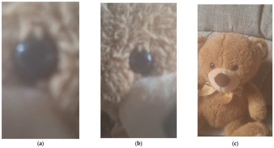
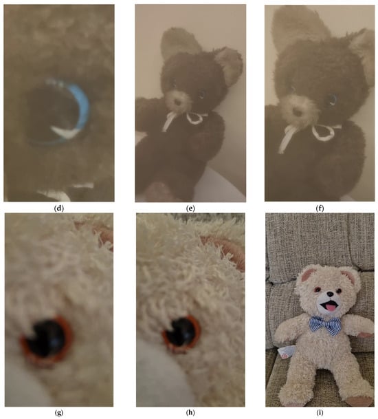
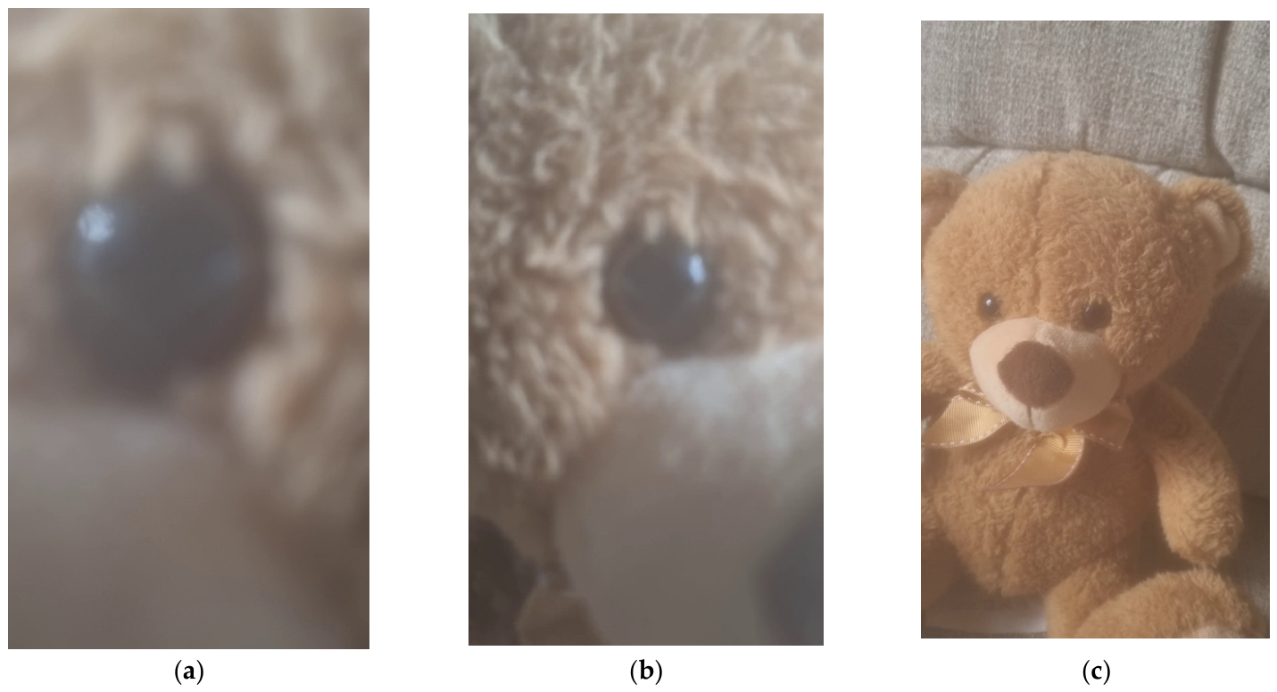
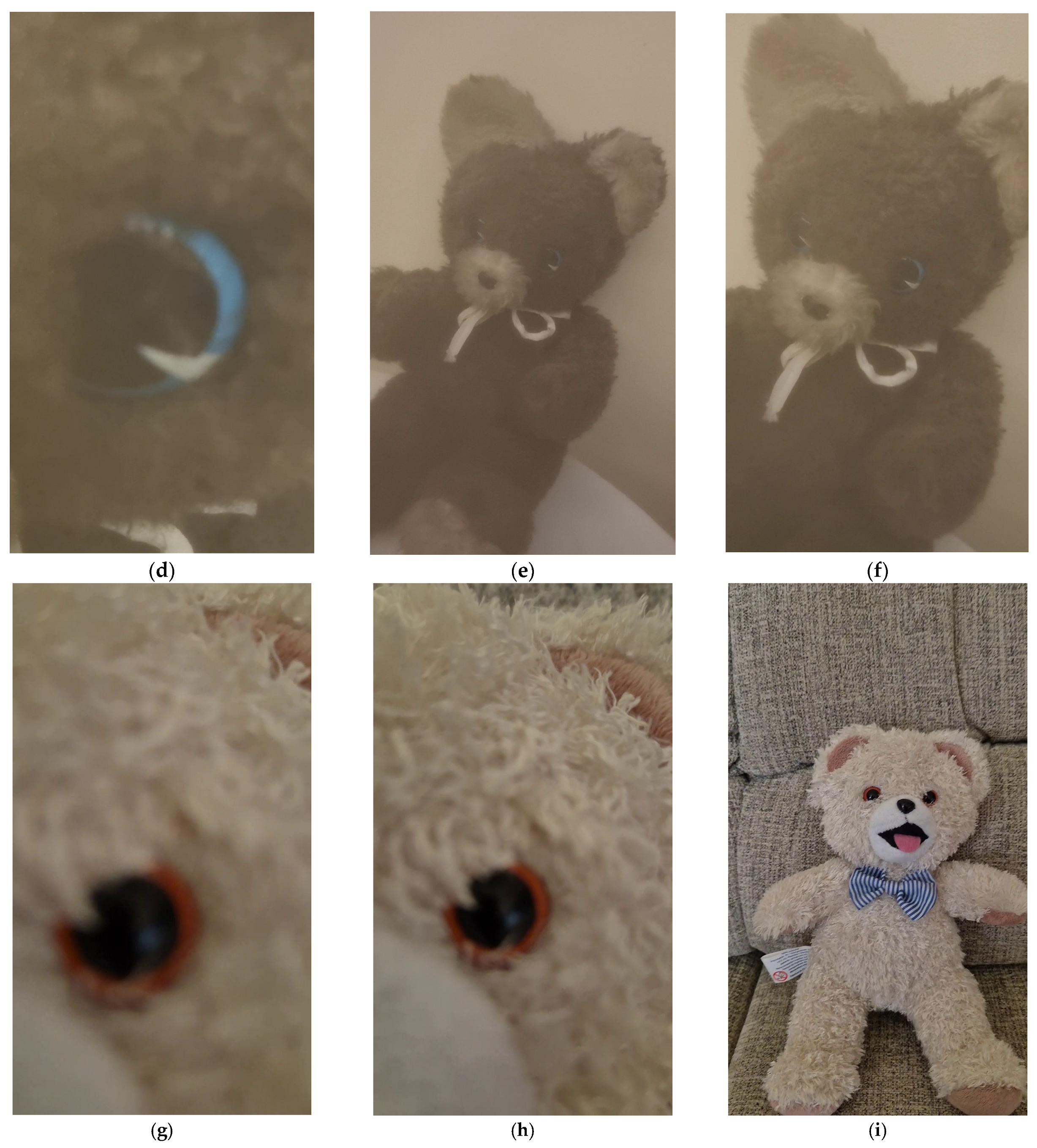
The first experiment analyzes three video sequences in which an object is filmed first from an extreme close-up and then from progressively greater distances, with the objective of identifying, in each sequence, the frame from which the object is correctly recognized. In all three the object is a plush teddy bear, whose canonical ImageNet label is teddy, teddy bear. The three sequences were selected to contrast acquisition conditions: Sequence 1 is a good-quality recording of a light-brown bear; Sequence 2 is a good-quality recording of a differently colored (gray) bear, which is the visually hardest case; and Sequence 3 (informally named “Coco”) is a lower-quality, longer recording. In each sequence the initial frames are so close that only a local texture (the fabric around the eye) is visible, which is a strong source of aleatoric uncertainty and is known to inflate softmax confidence without any underlying gain in information [1,3]. This protocol, and the similarity-based uncertainty indicator on which it relies, extend our earlier study [15].

5.2. Experimental Frame Extraction

Frames were extracted uniformly from each recorded sequence (about 71 frames for Sequences 1 and 2 and a longer run for Sequence 3). Figure 1 presents representative frames: for each sequence, the first frame (an extreme close-up in which only local texture is visible), an intermediate frame around which correct recognition begins, and the final frame, in which the whole object is visible.

Figure 1. Representative frames of the three teddy bear sequences. Top row, Sequence 1 (light-brown bear, good quality): (a) frame 1, an extreme close-up in which only the eye and the surrounding fabric are visible; (b) frame 15, from which correct recognition begins; (c) frame 71, the full object. Middle row, Sequence 2 (gray bear, differently colored): (d) an extreme close-up in which only the eye is visible; (e) an intermediate frame from which correct recognition begins; (f) the full object. Bottom row, Sequence 3 (“Coco”, lower quality): (g) frame 1; (h) frame 14, from which correct recognition begins; (i) frame 165, the full object.

5.3. Classification with a Pretrained VGG16 Backbone

A pretrained CNN was used to classify each extracted frame. For every sequence, a table was generated containing, for each frame, the two highest-ranked classes returned by the network (each with its class identifier, label, and probability) and stored as Pandas data frames that served as the primary data source for the subsequent processing stage. The VGG16 architecture was employed for classification [23]. VGG16 was developed by the Visual Geometry Group at the University of Oxford in 2014, accepts input images of size 224 × 224 × 3 pixels, and comprises 16 trainable layers; it was trained on ImageNet [24] and is distributed as a standard pretrained model in the TensorFlow/Keras Applications module. Because of its robust feature-extraction capabilities and standardized architecture, VGG16 remains a competitive and reproducible backbone, and ImageNet pretraining is known to transfer effectively to small downstream recognition tasks [25,26]. VGG16 is also a deliberately conservative choice for the present purpose: the abstention rule operates only on the two highest softmax outputs and is, in principle, backbone-agnostic, while a network that is known to be poorly calibrated provides an honest test case for a mechanism whose task is precisely to detect unreliable predictions.

Two observations from the recent literature motivated keeping the two highest probabilities rather than only the winning one. First, the softmax outputs of pretrained CNNs are miscalibrated (a high top-1 probability does not by itself certify a correct decision), so the margin between the top two classes is a more informative confidence signal than the top-1 value alone [1,3]. Second, that margin is the natural input to the possibilistic similarity function of Equation (5).

6. Results

6.1. Probability Trajectories

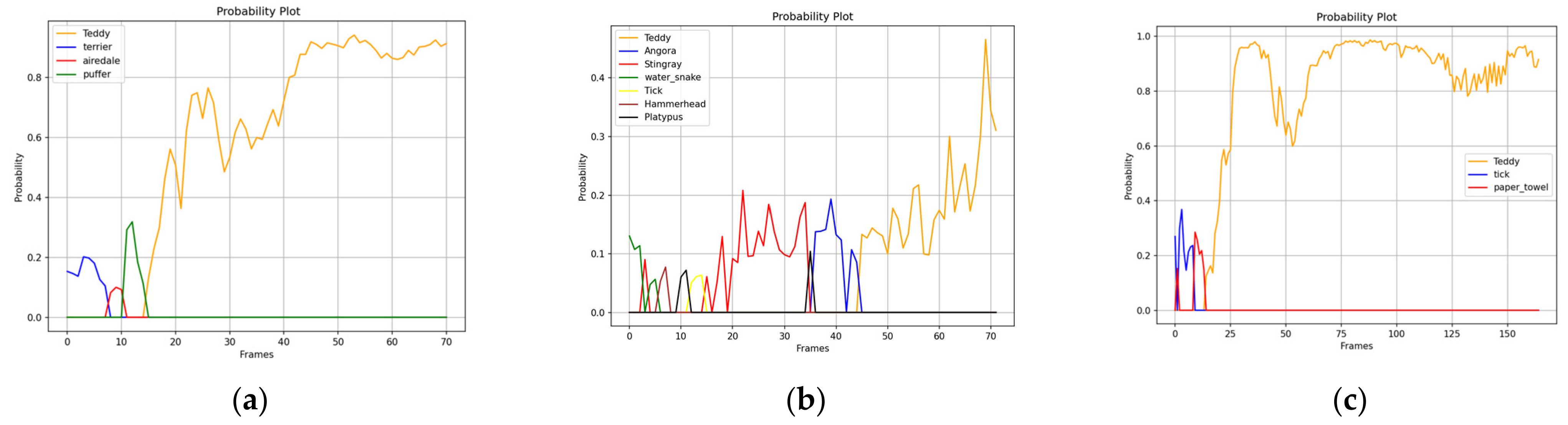
Figure 2 shows the probability values of the winning classes for the three sequences. In every sequence, incorrect classifications are observed at the beginning, when the image is acquired from an excessively short distance and does not contain enough distinctive features for accurate recognition. In Sequence 1 the classifier first selects terrier and pufferfish and switches to the correct teddy bear class from about frame 15, after which the winning probability rises above 0.9. In Sequence 2 (the differently colored bear) the confusion is far more severe and persistent: the classifier cycles through stingray, Angora, tick, hammerhead, and platypus, and the correct teddy bear class only takes the lead from about frame 42, and even then, with a low probability (at most about 0.47). In Sequence 3 the initial labels are tick and paper towel. The close-up is dominated by the dark, round eye and the light, fuzzy fabric, two ImageNet classes with a locally similar texture, and the correct label emerges from about frame 14, stabilizing between roughly 0.8 and 0.98.

Figure 2. Probability values of the winning classes for (a) Sequence 1, (b) Sequence 2, and (c) Sequence 3.

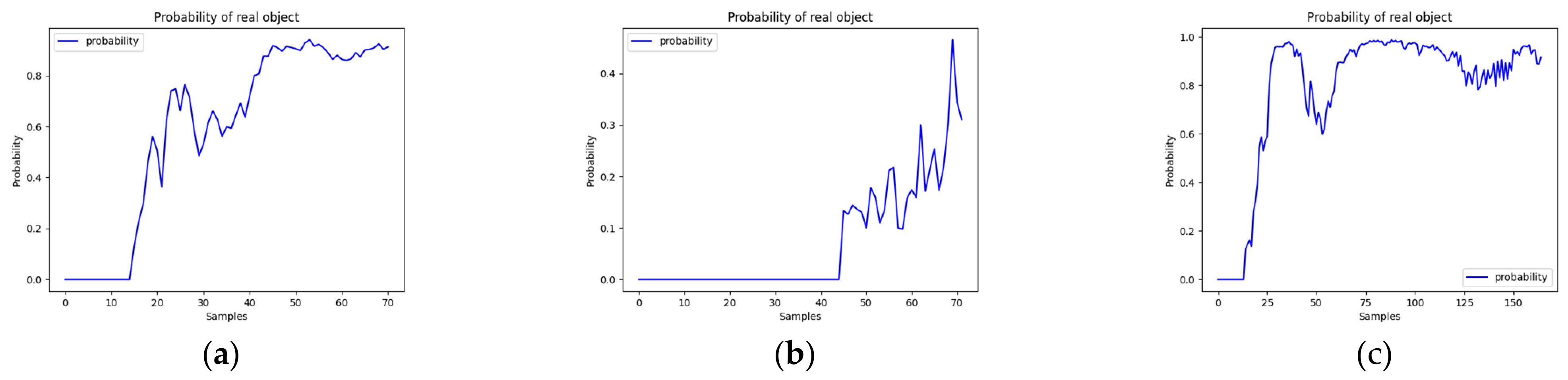
The appropriate outcome, while the prediction is wrong, would be for the system to indicate that the available visual information is insufficient to support a reliable decision. Figure 3 shows the probability assigned to the correct class across each sequence. During the initial close-up frames, the correct label is not even among the three highest-ranked predictions: precisely the failure mode that recent calibration work attributes to softmax over-confidence on out-of-distribution-like inputs [1,3]. The contrast between Sequences 1 and 3, in which the correct probability recovers to a high plateau, and Sequence 2, in which it remains low and noisy, quantifies the difficulty of the differently colored object.

Figure 3. Probability assigned to the correct class (teddy bear) for (a) Sequence 1, (b) Sequence 2, and (c) Sequence 3.

6.2. Threshold Estimation—Two-Variable Scenario

To determine the threshold, or transition interval, beyond which classification becomes reliable, two scenarios were analyzed. The first scenario acts as an ablation of the acquisition-distance term: it uses only the information contained in the softmax output, so the comparison with Section 6.3. isolates the contribution of the external geometric cue.

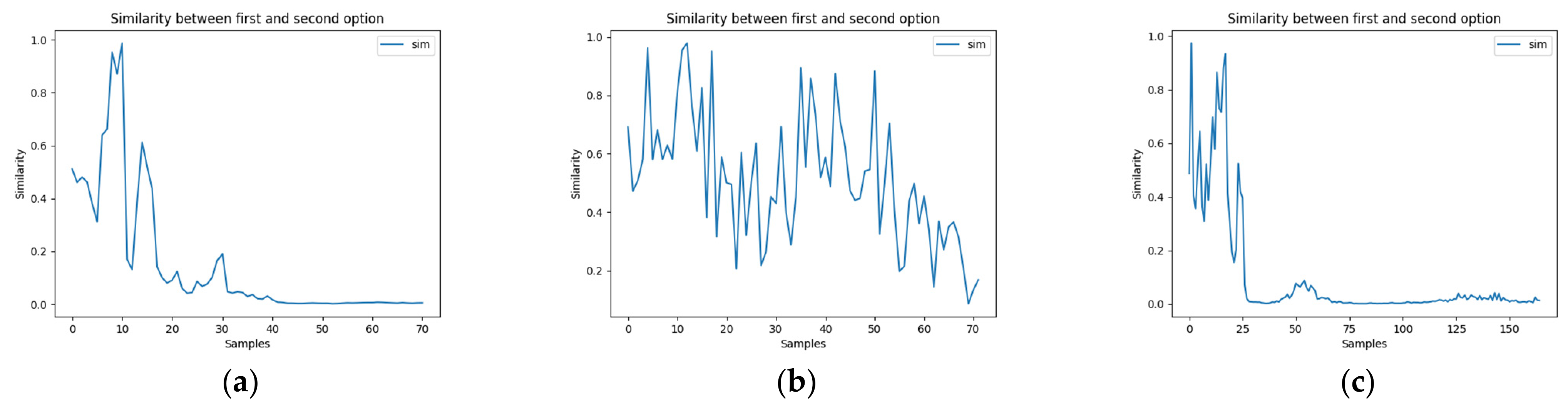
In the first scenario the possibility function was computed from two input variables: the fuzzy similarity between the first- and second-ranked candidates and the winning probability of each frame. The similarity was obtained with the relation of Section 2 (Equations (5) and (6)). Figure 4 presents the resulting similarity values. High similarity is observed at the beginning of each sequence, where the classification is highly uncertain, and it collapses toward zero once the object is recognized. Consistent with the difficulty of Sequence 2, its similarity remains high over a much larger portion of the sequence, indicating a persistently greater degree of confusability.

Figure 4. Fuzzy similarity between the first- and second-ranked classes for (a) Sequence 1, (b) Sequence 2, and (c) Sequence 3. Similarity stays high over a larger portion of Sequence 2.

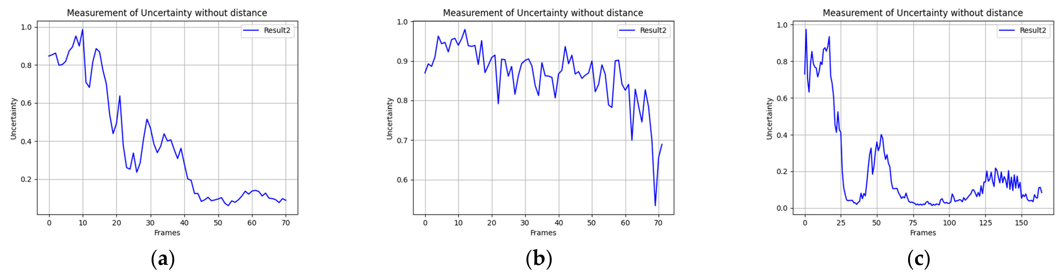
The possibility (uncertainty) function obtained in this two-variable scenario is shown in Figure 5. Uncertainty is high during the first close-up frames and drops as the object becomes recognizable, tracking the onset of correct recognition in each sequence; in Sequence 2 it remains elevated for most of the run, again reflecting the adverse acquisition conditions.

Figure 5. Possibility (uncertainty) function for the two-variable scenario (without the distance term) for (a) Sequence 1, (b) Sequence 2, and (c) Sequence 3.

6.3. Threshold Estimation: Three-Variable Scenario with Acquisition Distance

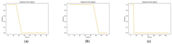
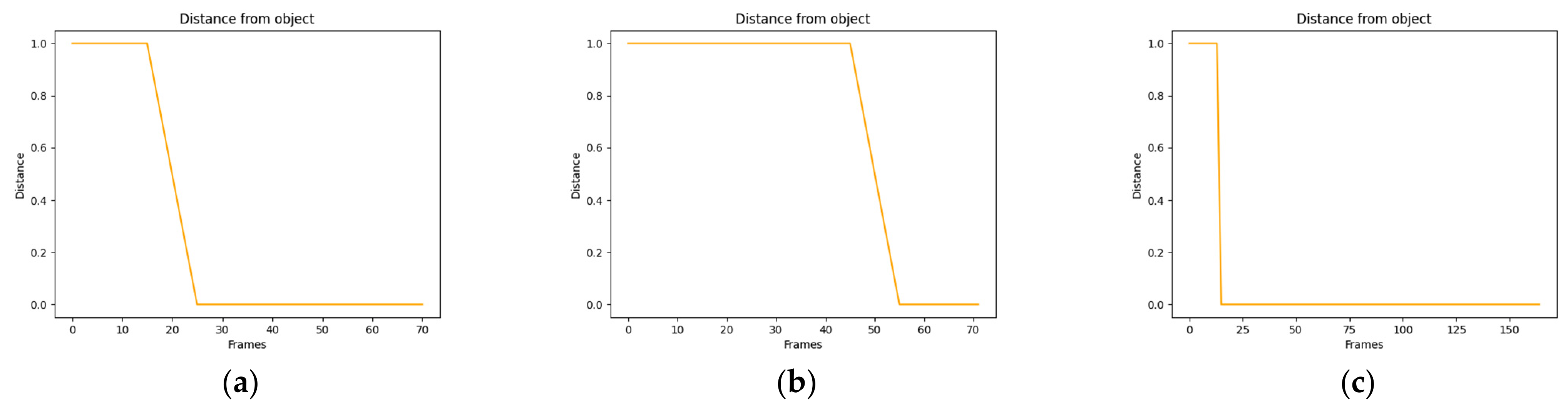
In the second scenario, information external to the video content was added in the form of a fuzzy function describing the object-to-camera distance. Figure 6 shows the corresponding fuzzy membership for the linguistic term very close: the membership equals one while the camera is extremely close to the object (the first frames, in which only local features are visible) and falls to zero as soon as the object is framed at a workable distance: around frame 25 for Sequences 1 and 3 and around frame 55 for Sequence 2. Treating acquisition geometry as an explicit input is consistent with the monocular depth-estimation and object-distance literature, in which the apparent size and geometric position of the object relative to the camera are recognized as standard geometric cues in monocular perception pipelines and are routinely fused with appearance features in safety-critical perception [27,28]. Modeling that cue as a coarse, ordinal fuzzy membership lets the method use an estimate that is cheap to obtain from a single camera, without a calibrated depth sensor.

Figure 6. Fuzzy membership function for the object-to-camera distance (linguistic term: very close) for (a) Sequence 1, (b) Sequence 2, and (c) Sequence 3.

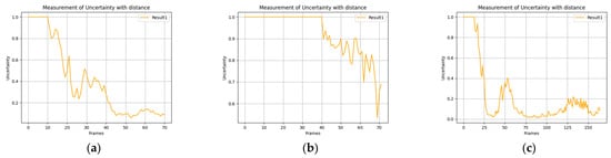
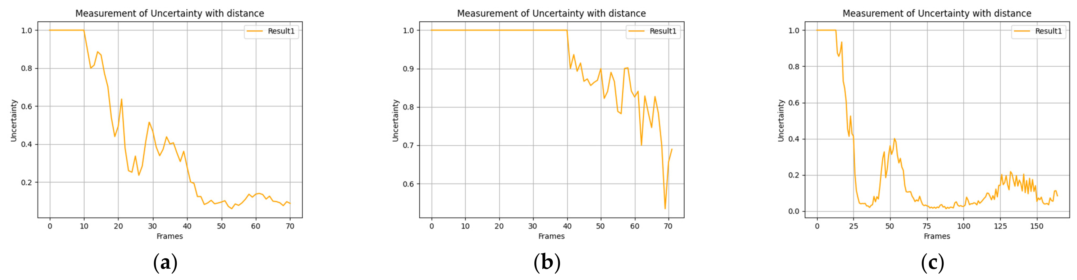
The possibility functions obtained when the three input variables are considered are presented in Figure 7. A clear improvement in the estimation of classification uncertainty is observed: in every sequence the frames from which the object is correctly recognized fall within the interval of increasing likelihood of correct prediction. The uncertainty is markedly lower and more stable when the classification is correct, whereas erroneous classifications are associated with high, strongly varying uncertainty. We deliberately avoid attaching fixed numeric cut-offs to these regimes, because the exact values depend on the acquisition conditions (e.g., illumination) even for the same object. Because the distance membership is one during the initial close-up frames, the three-variable possibility function is pinned at its maximum there, producing a cleaner high-uncertainty plateau at the start of each sequence and a sharper transition into the reliable-recognition region. For the hardest case, Sequence 2, the function correctly stays high over most of the run, so the method keeps signaling doubt precisely when the classifier cannot recover the correct label. This qualitative gain from adding a single geometric channel mirrors a finding now well established in the multimodal-fusion literature: fusing even one geometric or contextual channel with CNN appearance features materially improves recognition confidence under variable acquisition conditions, and fuzzy aggregation is one of the recurrently successful fusion strategies because it tolerates the imprecision of the auxiliary channel [28,29].

Figure 7. Possibility (uncertainty) function for the three-variable scenario (with the distance term) for (a) Sequence 1, (b) Sequence 2, and (c) Sequence 3. Correct-recognition frames correspond to a low, stable uncertainty, while erroneous frames correspond to high, strongly varying uncertainty.

6.4. Generalization Across Object Categories

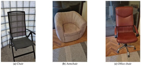
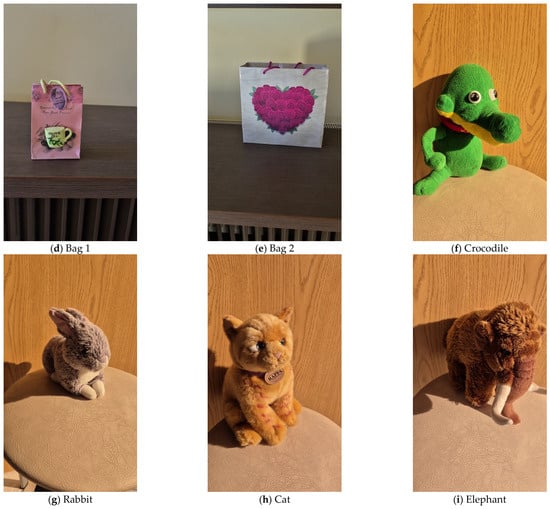
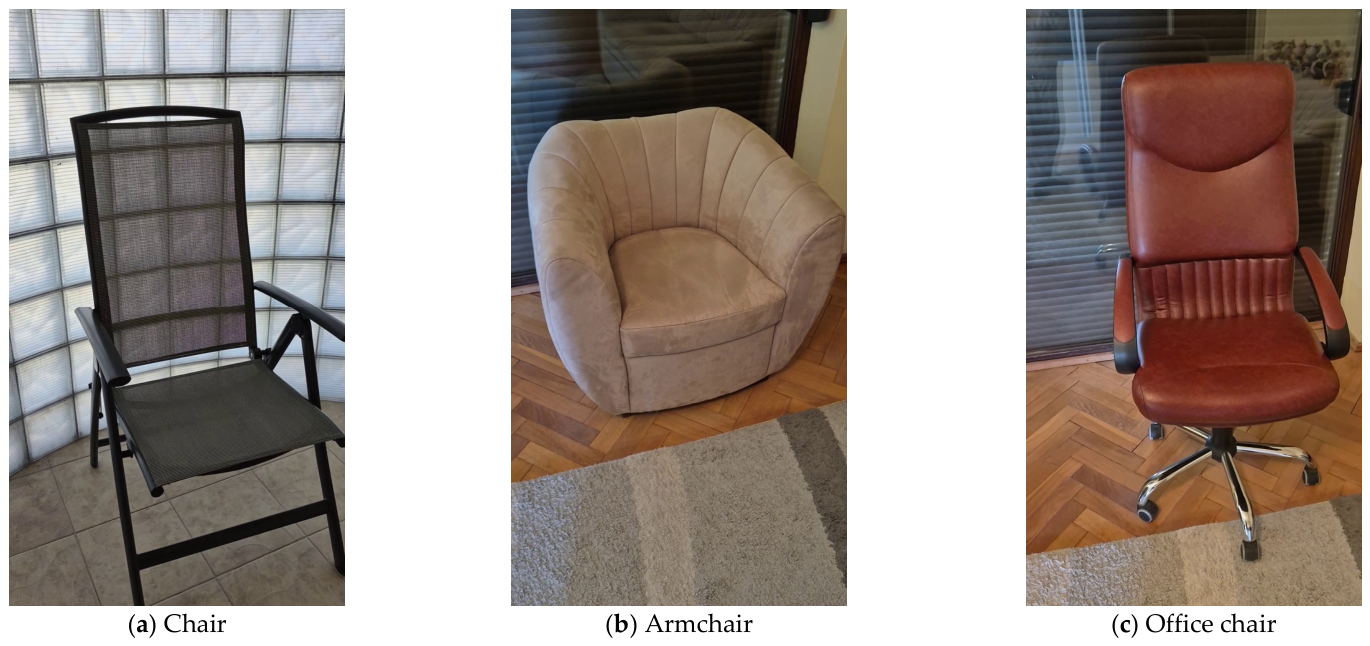
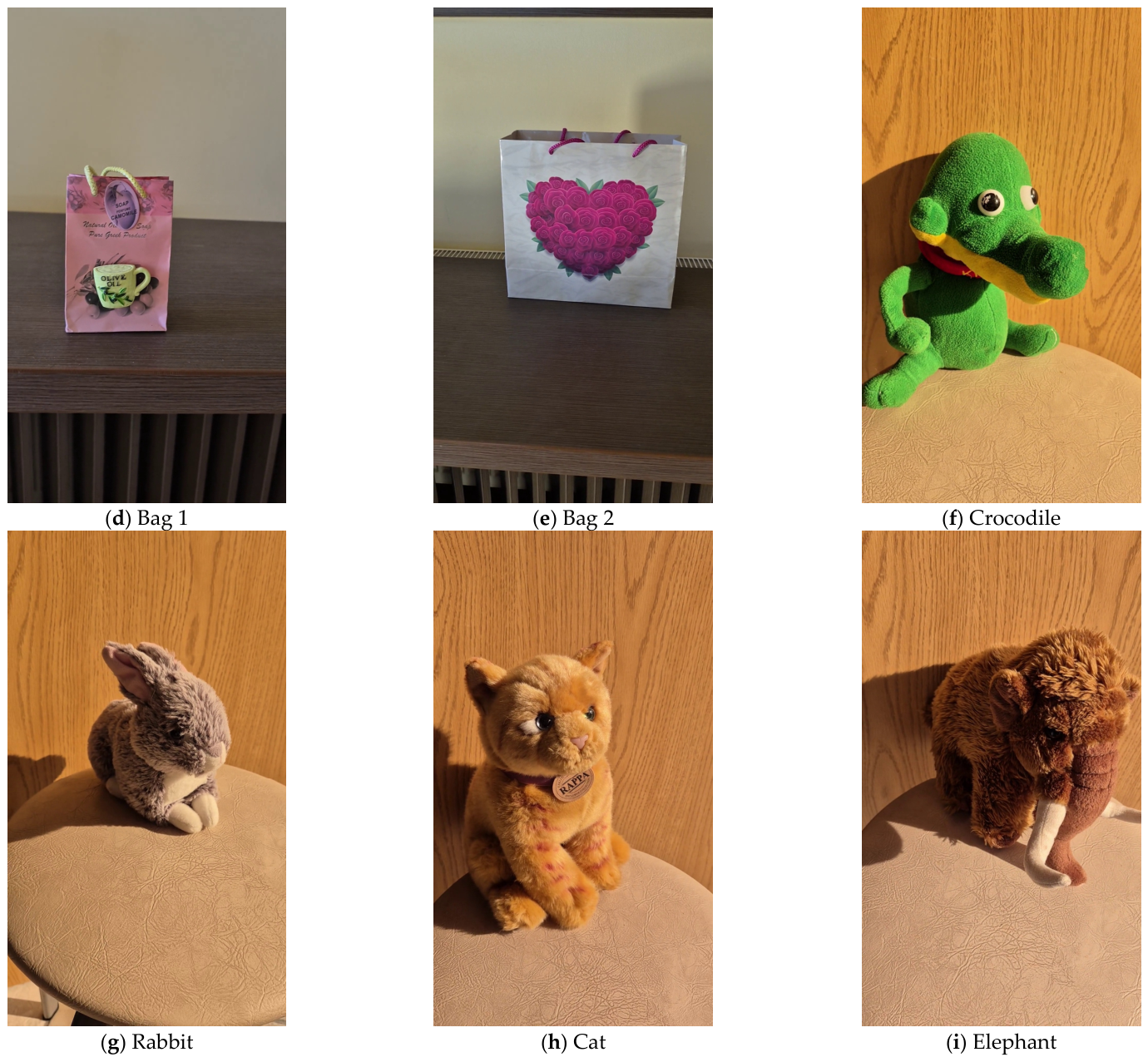
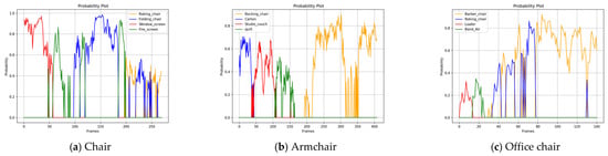
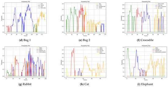
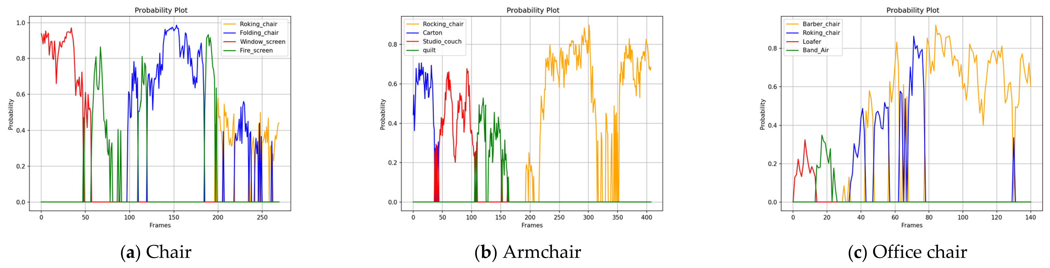
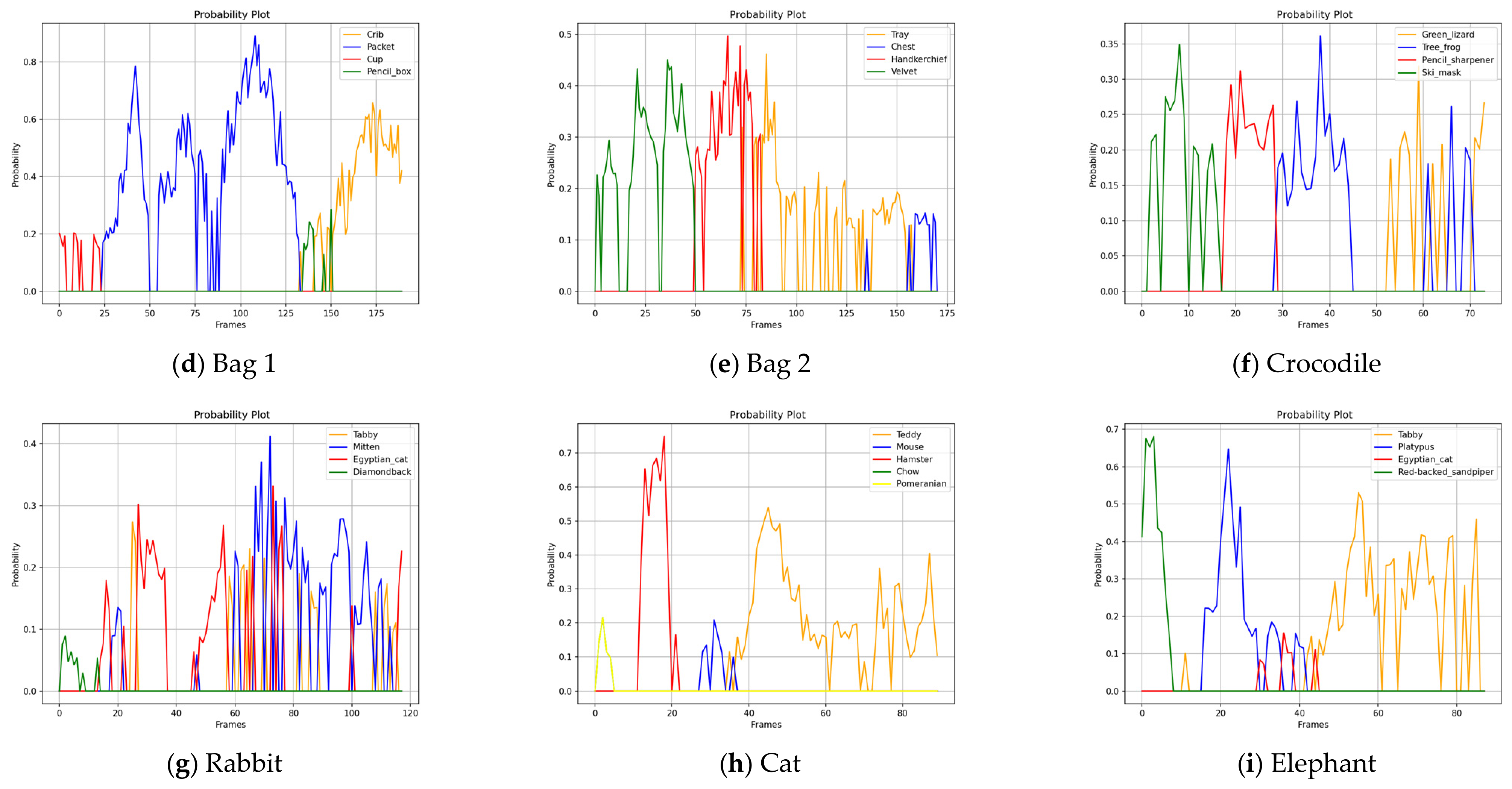
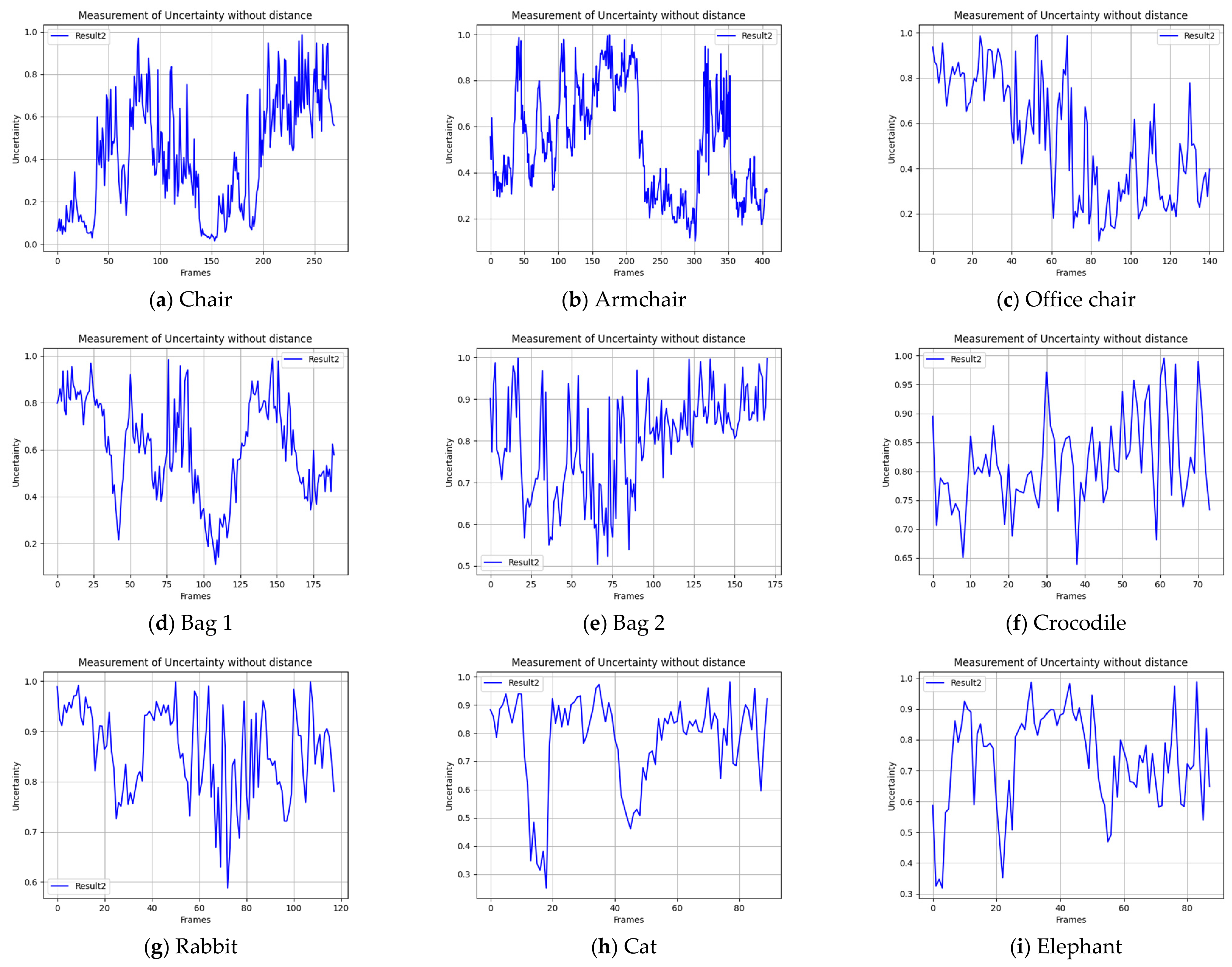
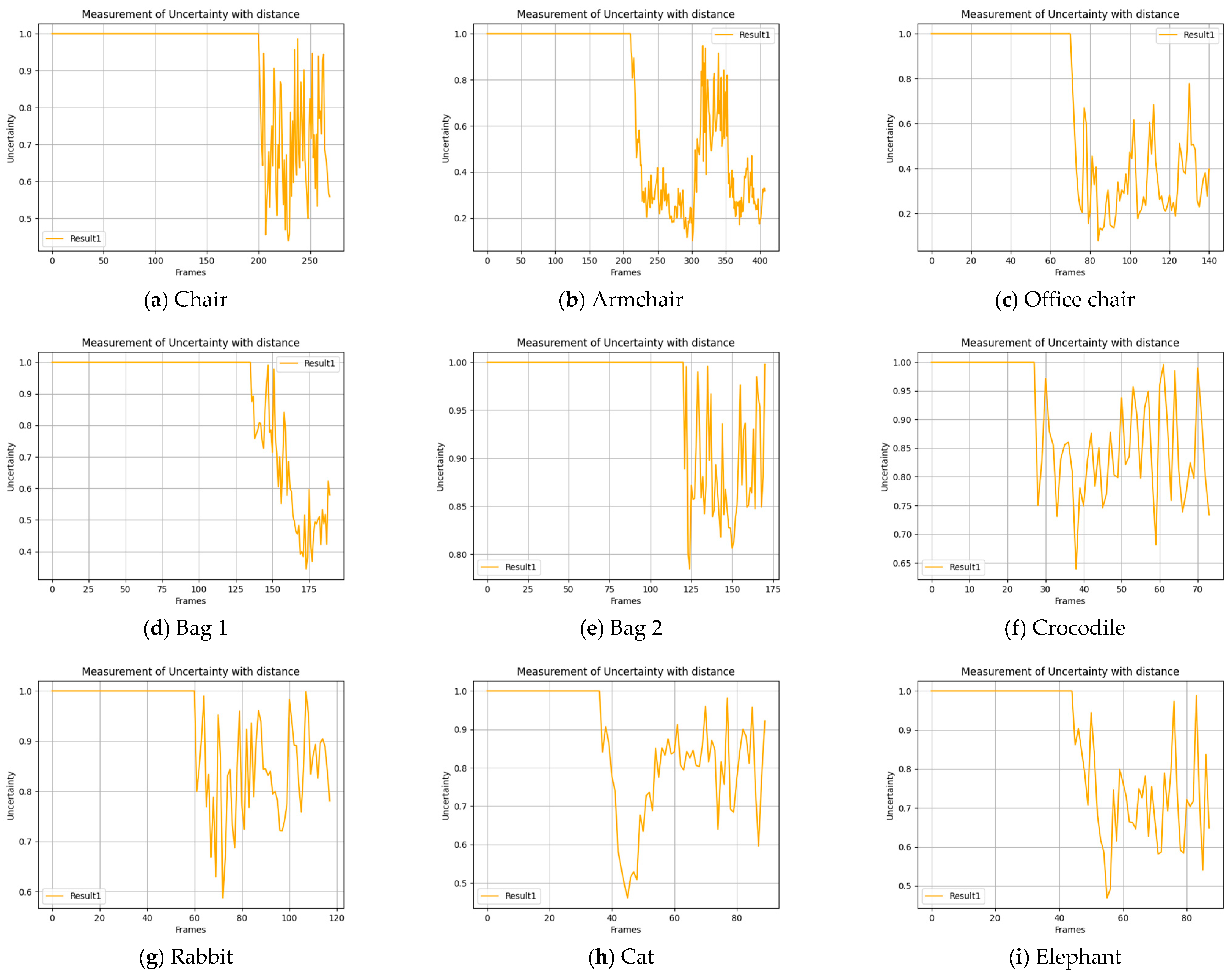
To assess whether the proposed abstention mechanism transfers beyond a single object category, the method was applied, with the same ImageNet-pretrained VGG16 backbone, to nine additional video sequences spanning three families: furniture (a chair, an armchair, and a leather office chair), deformable everyday objects (two bags), and plush animals (a crocodile, a rabbit, a cat, and an elephant). Each sequence follows the same acquisition protocol, from an extreme close-up to a full view. Figure 8 shows a representative frame of each object; Figure 9 shows the probability of the winning candidate classes; Figure 10 shows the possibilistic uncertainty without the acquisition-distance term (Result 2, the two-variable scenario without distance); and Figure 11 shows the uncertainty with the distance term (Result 1, the three-variable scenario with distance).

Figure 8. Representative frame (full object) of each additional sequence: (a) chair (folding_chair), (b) armchair (rocking_chair), (c) office chair (barber_chair), (d) bag 1 (packet), (e) bag 2 (tray), (f) crocodile (tree_frog), (g) rabbit (mitten), (h) cat (teddy), (i) elephant (tabby). The ImageNet class returned most often for each object is given in parentheses.

Figure 9. Probability of the winning candidate classes for the nine additional VGG16 sequences, in the order (a–i) as above. Early frames are dominated by unrelated classes; the correct class, when the backbone can recover it, takes the lead as the object comes fully into view.

Figure 10. Possibilistic uncertainty without the acquisition-distance term (Result 2) for the nine additional sequences, in the same order (a–i).

Figure 11. Possibilistic uncertainty with the acquisition-distance term (Result 1) for the nine additional sequences, in the same order (a–i). Low, stable values indicate reliable recognition; persistently high or strongly oscillating values indicate that the method abstains and reports an unidentified object.

Across these categories the uncertainty behaves exactly as the method prescribes. For objects that the backbone can place within an ImageNet class with a stable margin, such as the leather office chair, the uncertainty collapses to a low, steady regime once the object is in view. For objects that are intrinsically hard for an ImageNet model-in particular the plush animals, for which few doll-like categories exist in the label set-the uncertainty remains high and strongly oscillating throughout the sequence, so the method keeps abstaining rather than committing to a wrong label. This provides preliminary evidence, across object types, of a simple operational reading of the uncertainty trace: a consistently low value denotes a reliable recognition, whereas persistently high values or strong oscillations denote an unreliable decision that should be declared an unidentified object. We intentionally do not convert this reading into a single universal numeric threshold, because the exact levels depend on the acquisition conditions (e.g., illumination) even for the same object.

6.5. Application to a Second CNN Backbone (VGG16 Versus ResNet-50)

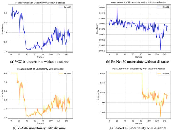
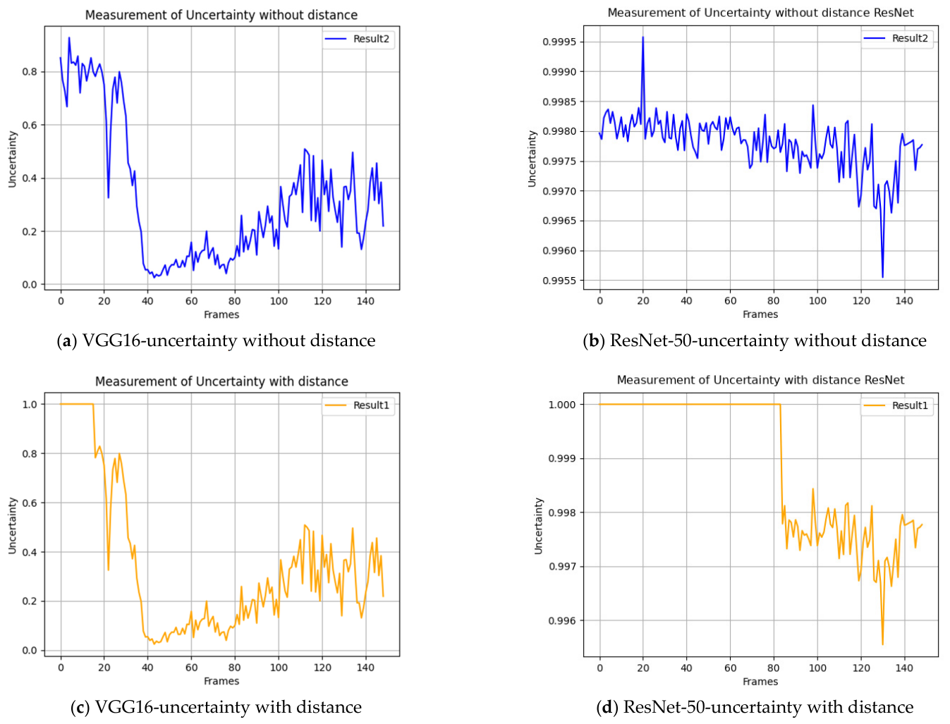
Because the rejection rule operates only on the two highest softmax outputs, it can be applied unchanged to any backbone. To illustrate this, the bear sequence was additionally processed with a ResNet-50 backbone. Figure 12 contrasts the two backbones, without and with the distance term. With VGG16 the uncertainty collapses once the object is in view, so the method accepts the label; with ResNet-50 the winning probability does not dominate on these sequences, and the uncertainty stays high, so the method keeps abstaining. This shows the rule operates unchanged on a second backbone and that its output tracks the reliability of the underlying classifier; a stronger demonstration of backbone-independent error selection would require a second backbone that reaches competitive accuracy on these sequences, which we note as a limitation.

Figure 12. Backbone comparison on the bear sequence: possibilistic uncertainty without (a,b) and with (c,d) the distance term, for VGG16 (a,c) and ResNet-50 (b,d). With ResNet-50 the uncertainty remains saturated near 1.0, so the method correctly abstains-the abstention rule operates unchanged on either backbone.

6.6. Quantitative Comparison with Confidence-Based Baselines

The preceding sections read the abstention behavior qualitatively. To complement this with a quantitative, reproducible evaluation, the sequences are split into two groups according to whether the backbone has a corresponding ImageNet class. For the recognizable objects-the three teddy bear sequences (correct class “teddy”) and the three chairs (ImageNet chair classes)-the task is selective classification: a reference (ground-truth) class is assigned to each object independently of the model and fixed before the evaluation; for each frame the backbone’s top-1 label is then compared against this reference, and the frame is counted correct only when the top-1 label is one of the reference classes: a semantically related prediction that falls outside them (for example, a chair returned as a non-chair furniture class) counting as incorrect. The per-sequence recognition error rates for the six recognizable sequences are summarized in Table 1.

Table 1. Recognition error on the six recognizable sequences, computed directly from the per-frame top-1 predictions (a frame is correct when its top-1 label equals the object’s ImageNet class). Recognition is wrong on the early frames, while the object is only partially in view, and becomes correct once it is fully framed.

Sequence	Frames	Correct ImageNet Class	Recognition Error (%)
Bear 1	71	teddy (teddy bear)	21.1
Bear 2	72	teddy (teddy bear)	62.5
Bear “Coco”	165	teddy (teddy bear)	8.5
Chair	270	ImageNet chair classes	45.2
Armchair	408	ImageNet chair classes	56.1
Office chair	141	barber chair	22.7

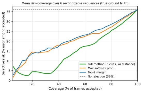
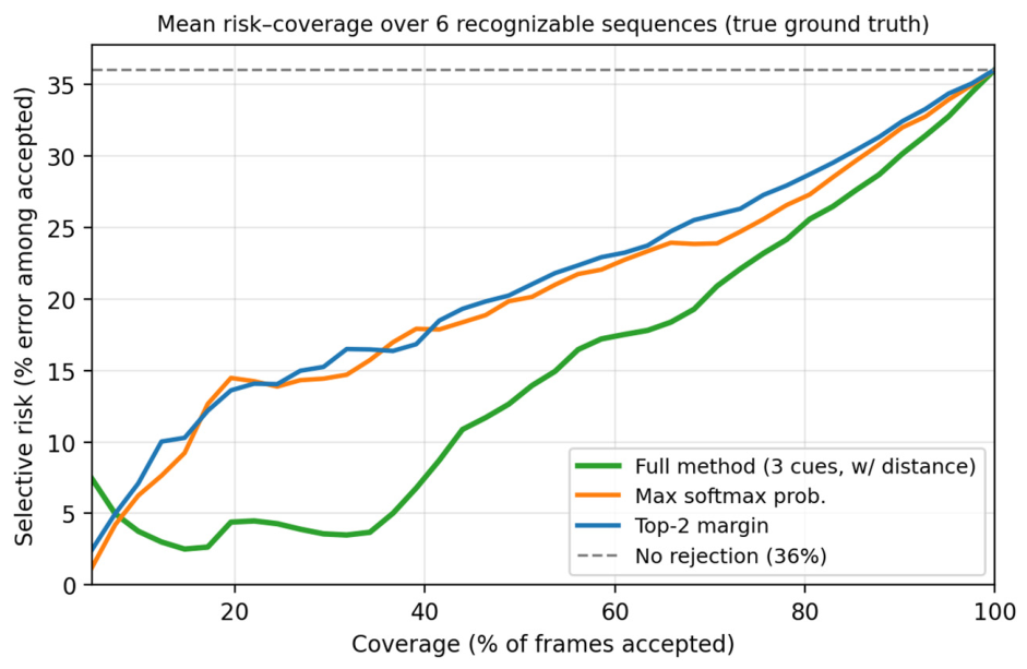
On this group we compare, on the same frames, four rejection scores: the maximum softmax probability (MSP = p₁), the top-two margin (p₁ − p₂), the possibilistic score that uses only the two softmax outputs, max(u_p, u_s) with u_p = 1 − p₁ and u_s = p₂/p₁, and the full possibilistic rule that additionally uses the acquisition-distance cue. Performance is the area under the per-sequence risk–coverage curve (AURC, lower is better) and the selective risk at fixed coverage (Table 2, Figure 13). For the remaining objects (two bags and four plush animals) there is no suitable ground-truth class under our labeling protocol: a frame is counted correct only when the top-1 label names the physical object, and a plush toy of an animal has no matching ImageNet class (nor does the backbone return the corresponding real-animal class). So, classification accuracy is not defined; there, the relevant question is whether the method abstains (Table 3).

Table 2. Selective-classification performance on the six recognizable sequences (mean over sequences; lower is better): area under the risk–coverage curve (AURC) and selective risk at fixed coverage. The full rule, which adds the acquisition-distance cue, outperforms the three softmax-only scores, which are close to one another because they are all functions of the two leading probabilities.

Method	AURC (↓)	Risk@50%	Risk@70%	Risk@80%	Risk@90%
Full possibilistic rule (3 cues)	0.148	13.0	20.4	25.4	30.0
Max softmax probability (MSP)	0.195	19.6	23.9	27.2	31.9
Top-two margin (p1−p2)	0.203	20.0	25.8	28.7	32.2
Possibilistic, no distance (2 cues)	0.198	19.9	25.1	28.1	32.2
No rejection (base error)	0.360	36.0	36.0	36.0	36.0
Oracle (errors rejected first)	0.106	–	–	–	–

Figure 13. Mean risk–coverage curves over the six recognizable sequences (true per-frame ground truth). The full possibilistic rule (with the acquisition-distance cue) lies below the maximum softmax probability and the top-two margin across the operating range, and its advantage widens as more frames are rejected. “No rejection” marks the mean base error.

Table 3. Objects without a suitable ground-truth class under the adopted labeling protocol: a plush toy of an animal and the two bags have no matching ImageNet class, so the top-1 label is never correct, and classification accuracy is not defined. The table lists the class the top-1 prediction drifts to. On every such sequence the possibilistic uncertainty of the full rule remains high throughout and never settles into the low, stable regime observed for recognized objects, so the method abstains rather than committing to a label: the intended behavior for objects outside the label set.

Sequence	Frames	Top-1 Drifts to
Bag (mug)	190	crib/packet
Bag (heart)	171	tray/packet
Crocodile	74	green lizard/tree frog
Rabbit	118	mitten/Egyptian cat
Cat	90	teddy
Elephant	88	tabby/toy poodle

Two findings stand out. First, on the objects the backbone can recognize, the full possibilistic rule is the most effective at ordering frames for abstention: its mean AURC (0.148) is clearly below the maximum softmax probability (0.195), the top-two margin (0.203) and the softmax-only possibilistic score (0.198), and its advantage widens as more frames are rejected-at 50% coverage the selective risk falls to 13.0%, against 19.6% for the maximum softmax probability (Table 2, Figure 13). The three softmax-based scores are close to one another, as expected since they are all functions of the two leading probabilities; the improvement of the full rule therefore comes specifically from the acquisition-distance cue, which flags the close-range frames in which the classifier is confidently wrong and which the softmax scores accept. Second, for the objects without a suitable ground-truth class, the full-method uncertainty stays high throughout and never settles into the low, stable regime seen for recognized objects (Table 3), so the method abstains rather than emitting a wrong label-the intended behavior when the object lies outside the label set. Per sequence (Table 4), the full rule is best on five of the six sequences (the exception being the office chair, where it is within 0.015 AURC of the best), confirming the gain is consistent rather than driven by one sequence. With only six heterogeneous sequences, we report this per-sequence breakdown (Table 4) rather than a formal significance test; the mean improvement over the maximum softmax probability is ΔAURC ≈ 0.047 (full rule versus MSP), consistent in sign on five of the six sequences.

Table 4. Per-sequence AURC (lower is better) for each rejection score on the six recognizable sequences. The full rule attains the lowest AURC on five of the six sequences, so the improvement is not driven by a single sequence.

Sequence	MSP	Top-2 Margin	No Distance	Full Rule
Bear 1	0.027	0.027	0.027	0.025
Bear 2	0.353	0.353	0.353	0.258
Bear Coco	0.006	0.006	0.006	0.004
Chair	0.480	0.495	0.478	0.338
Armchair	0.271	0.276	0.273	0.214
Office chair	0.036	0.060	0.050	0.051

A note on the acceptance threshold η is in order. The risk–coverage curves above evaluate, retrospectively, how well each score orders predictions by risk; they do not by themselves prescribe a value of η for a new application. In deployment η must be selected on a separate validation set, before testing, to meet a target coverage or selective risk; the present results therefore establish the discriminative quality of the possibilistic score rather than a universal numeric threshold.

Finally, we consider the manually set breakpoints of the distance-membership function. Because the distance term enters only through the maximum operator, Π = max(u_p, u_d, u_s), changing the breakpoints cannot make the full rule accept a label that the distance-free rule would reject; it can only add abstention. It can, however, change how many frames are rejected, and therefore the coverage and the selective risk, so we do not claim the decision is invariant to the breakpoints. The two configurations reported here bound the range of this influence: with the distance term switched off (Result 2, Figure 10) and with it fully active (Result 1, Figure 11); in both, the recognizable objects are accepted once in full view, and the out-of-vocabulary objects are abstained on. The breakpoints are set from the physical acquisition geometry (the near distance at which the object overflows the field of view and the far distance at which it is fully framed) rather than tuned on the results. A systematic sweep of the breakpoints would quantify their effect on coverage and selective risk exactly and requires the per-frame acquisition distances; the present experiments bound that effect rather than sweeping it.

7. Discussion

The experiments support the central claim of the paper: a qualitative, possibilistic aggregation of three cheap indicators reproduces, on real video, the abstention boundary that statistical selective-classification methods would otherwise recover only with a calibrated confidence model and a held-out calibration set [8,13,20]. Across all three sequences the transition to a low, stable uncertainty coincides with the onset of correct recognition, while erroneous classifications keep the uncertainty high and strongly varying. We do not attach a fixed numeric band to this transition: the exact values shift with the acquisition conditions (for instance, illumination) even for the same object, so the uncertainty is best read as a relative decision signal rather than an absolute threshold. Sequence 2 is particularly informative: because the differently colored bear is genuinely hard for the backbone, the possibility function correctly remains high for most of the run, which is the desired behavior: an abstention mechanism should keep refusing when the evidence never becomes sufficient. It should be noted that in Sequence 2 the mechanism also abstains on a number of frames for which the classifier does return the correct label. Because the winning probability there never exceeds approximately 0.47, this is the expected behavior of a conservative maximum t-conorm, but it illustrates the coverage cost of the aggregation: reliability on the accepted set is obtained at the price of rejecting predictions that happen to be correct yet weakly supported.

The method has three practical strengths. It is interpretable, because every abstention can be explained by the activated fuzzy rules and by which of the three indicators dominated the maximum; it is lightweight, because it reuses a single forward pass and adds only a small fuzzy-inference step; and it is conservative, because the maximum t-conorm abstains as soon as any indicator signals danger. These properties make it attractive for resource-constrained or auditable deployments, where the multiple forward passes of Bayesian or ensemble methods [5,6] are impractical. This positioning is consistent with the broader literature on fuzzy components inside deep architectures, which reports that a fuzzy decision layer is most useful precisely where interpretability and low inference cost matter more than a calibrated posterior [30,31].

Several limitations should be acknowledged. The uncertainty produced by the method is qualitative and ordinal rather than a calibrated probability, which is appropriate when the evidence itself is sparse but does not, on its own, provide a finite-sample coverage guarantee. Whether such an ordinal measure is preferable to an explicitly epistemic one remains an open question: the distinction between aleatoric and epistemic uncertainty is central to modern uncertainty quantification [32], and evidential classifiers built on Dempster–Shafer theory offer a closely related, set-based alternative to the possibilistic reading adopted here [33].

The acceptance threshold η is currently set by the designer rather than learned. In addition, the method does not commit to a fixed numeric acceptance band: we found that such a cut-off depends on the acquisition conditions (for instance, illumination) even for the same object, so the acceptance threshold η is treated as a tunable operating point, set per application, rather than as a universal constant.

Several limitations should be stated explicitly. First, all sequences follow the same acquisition protocol, in which the camera moves from an extreme close-up to a full view; the acquisition-distance indicator therefore benefits from a correlation built into the protocol, because the early, hard-to-recognize frames are also the close-range ones. The improvement attributed to the distance cue should accordingly be read within this protocol and need not transfer to settings in which a fully framed object is still misclassified. Second, the acquisition-distance indicator assumes a measurable camera-to-object geometry; in a deployed system it could be supplied automatically (for example by an inexpensive ultrasonic range sensor or a monocular-depth estimate), but we did not evaluate the method with an automatically estimated distance, and we did not carry out a sensitivity analysis of the distance-membership breakpoints (for example ±10 − 20% changes); both require the per-frame distances and remain to be validated experimentally. Third, the acceptance threshold η is an operating-point choice: the risk–coverage curves evaluate how well each score orders predictions by risk, and in a new application η must be selected on a separate validation set before testing rather than read from the test data. Fourth, the second backbone (ResNet-50) did not reach a competitive accuracy on these sequences, so backbone independence is demonstrated only at the procedural level. Finally, the stated application areas, such as medical screening support and assisted driving, are potential applications rather than validated use cases.

8. Conclusions

This paper presented a lightweight abstention mechanism for convolutional neural networks that models classification uncertainty with fuzzy logic and possibility theory, aggregating the complement of the winning probability, a fuzzy similarity between the two top-ranked classes and, optionally, an object-to-camera distance cue, without retraining the classifier. The mechanism was evaluated on twelve video sequences spanning several object categories and with two CNN backbones. On the objects for which the backbone has a corresponding ImageNet class, a quantitative risk–coverage analysis showed that the full possibilistic rule orders predictions for abstention better than the maximum-softmax-probability and top-two-margin baselines (mean AURC 0.148 versus 0.195 and 0.203), with the improvement attributable to the distance cue; on objects without a suitable ground-truth class, the rule abstained rather than emitting a wrong label. These results provide preliminary evidence that a qualitative, interpretable possibilistic rule can reproduce, on real video, the abstention behavior targeted by statistical selective-classification methods, without a held-out calibration set; the limitations noted above indicate the validation still required before general deployment claims can be made.

Three directions are open for future work. First, the possibility threshold η is currently set by the designer; learning it from a labeled validation set, in the spirit of the joint training of classifier and rejection function in SelectiveNet, would remove the only hand-tuned hyper-parameter of the method. Second, the acquisition-distance indicator could be replaced by a learned monocular depth estimate produced by a general-purpose depth foundation model [34], extending the method to unconstrained imagery. Third, the qualitative necessity threshold could be wrapped by a downstream conformal-prediction layer over the accepted set, combining the interpretability of the possibilistic abstention with the finite-sample coverage guarantee of conformal prediction. Validation on additional object categories and backbones is also planned to establish the generality of the approach.

References

- Guo, C.; Pleiss, G.; Sun, Y.; Weinberger, K.Q. On calibration of modern neural networks. In Proceedings of the 34th International Conference on Machine Learning (ICML), Sydney, Australia, 6–11 August 2017; Volume 70, pp. 1321–1330. [Google Scholar]
- Hendrycks, D.; Gimpel, K. A baseline for detecting misclassified and out-of-distribution examples in neural networks. In Proceedings of the 5th International Conference on Learning Representations (ICLR), Toulon, France, 24–26 April 2017. [Google Scholar]
- Pearce, T.; Brintrup, A.; Zhu, J. Understanding softmax confidence and uncertainty. arXiv 2021, arXiv:2106.04972. [Google Scholar] [CrossRef] [Scilit]
- He, W.; Jiang, Z.; Xiao, T.; Xu, Z.; Li, Y. A survey on uncertainty quantification methods for deep learning. ACM Comput. Surv. 2026, 58, 1–35. [Google Scholar] [CrossRef] [Scilit]
- Gal, Y.; Ghahramani, Z. Dropout as a Bayesian approximation: Representing model uncertainty in deep learning. In Proceedings of the 33rd International Conference on Machine Learning (ICML), New York, NY, USA, 19–24 June 2016; Volume 48, pp. 1050–1059. [Google Scholar]
- Lakshminarayanan, B.; Pritzel, A.; Blundell, C. Simple and scalable predictive uncertainty estimation using deep ensembles. In Proceedings of the Advances in Neural Information Processing Systems 30 (NeurIPS), Long Beach, CA, USA, 4–9 December 2017; pp. 6405–6416. [Google Scholar]
- Sensoy, M.; Kaplan, L.; Kandemir, M. Evidential deep learning to quantify classification uncertainty. In Proceedings of the Advances in Neural Information Processing Systems 32 (NeurIPS), Montréal, QC, Canada, 3–8 December 2018; pp. 3179–3189. [Google Scholar]
- Angelopoulos, A.N.; Bates, S. Conformal prediction: A gentle introduction. Found. Trends Mach. Learn. 2023, 16, 494–591. [Google Scholar] [CrossRef] [Scilit]
- Ni, Y.; Houssineau, J.; Ong, Y.-S.; Koniusz, P. Possibilistic predictive uncertainty for deep learning. In Proceedings of the 43rd International Conference on Machine Learning (ICML), Seoul, Republic of Korea, 6–11 July 2026. [Google Scholar] [CrossRef] [Scilit]
- Chow, C. On optimum recognition error and reject tradeoff. IEEE Trans. Inf. Theory 1970, 16, 41–46. [Google Scholar] [CrossRef] [Scilit]
- Geifman, Y.; El-Yaniv, R. SelectiveNet: A deep neural network with an integrated reject option. In Proceedings of the 36th International Conference on Machine Learning (ICML), Long Beach, CA, USA, 9–15 June 2019; Volume 97, pp. 2151–2159. [Google Scholar]
- Franc, V.; Prusa, D.; Voracek, V. Optimal strategies for reject option classifiers. J. Mach. Learn. Res. 2023, 24, 1–49. [Google Scholar]
- Hendrickx, K.; Perini, L.; Van der Plas, D.; Meert, W.; Davis, J. Machine learning with a reject option: A survey. Mach. Learn. 2024, 113, 3073–3110. [Google Scholar] [CrossRef] [Scilit]
- Dubois, D.; Prade, H. Possibility theory and its applications: Where do we stand? In Springer Handbook of Computational Intelligence; Kacprzyk, J., Pedrycz, W., Eds.; Springer: Berlin/Heidelberg, Germany, 2015; pp. 31–60. [Google Scholar] [CrossRef] [Scilit]
- Barna, C.; Petcut, F.-M.; Petcut-Lasc, A.-A. Similarity measurement of uncertainty in artificial neural networks classification. In Proceedings of the 2025 IEEE 19th International Symposium on Applied Computational Intelligence and Informatics (SACI), Timisoara, Romania, 19–24 May 2025; pp. 327–330. [Google Scholar] [CrossRef] [Scilit]
- Zadeh, L.A. Fuzzy sets. Inf. Control 1965, 8, 338–353. [Google Scholar] [CrossRef] [Scilit]
- Zadeh, L.A. Fuzzy sets as a basis for a theory of possibility. Fuzzy Sets Syst. 1978, 1, 3–28. [Google Scholar] [CrossRef] [Scilit]
- Ullah, T.; Ullah, K.; Khan, P.; Brikova, O.; Voznesensky, A.; Eroshkin, A.; Hussain, I. Fuzzy logic and deep learning approach for automated white blood cell detection and classification via multi-CNN feature fusion. Sci. Rep. 2025, 15, 44546. [Google Scholar] [CrossRef] [Scilit] [PubMed]
- Bargiela, A.; Pedrycz, W.; Hirota, K. Logic-based granular prototyping. In Proceedings of the 26th Annual International Computer Software and Applications Conference (COMPSAC 2002), Oxford, UK, 26–29 August 2002; pp. 1164–1169. [Google Scholar] [CrossRef] [Scilit]
- Pugnana, A.; Perini, L.; Davis, J.; Ruggieri, S. Deep neural network benchmarks for selective classification. J. Data-Centric Mach. Learn. Res. 2024. Available online: https://openreview.net/pdf?id=xDPzHbtAEs (accessed on 5 September 2026).
- Gangrade, A.; Kag, A.; Saligrama, V. Selective classification via one-sided prediction. In Proceedings of the 24th International Conference on Artificial Intelligence and Statistics (AISTATS), Virtual, 13–15 April 2021; Volume 130, pp. 2179–2187. [Google Scholar]
- Liang, H.; Peng, L.; Sun, J. Selective classification under distribution shifts. Trans. Mach. Learn. Res. 2024, 2024, dmxMGW6J7N. [Google Scholar]
- Simonyan, K.; Zisserman, A. Very deep convolutional networks for large-scale image recognition. In Proceedings of the 3rd International Conference on Learning Representations (ICLR), San Diego, CA, USA, 7–9 May 2015. [Google Scholar]
- Russakovsky, O.; Deng, J.; Su, H.; Krause, J.; Satheesh, S.; Ma, S.; Huang, Z.; Karpathy, A.; Khosla, A.; Bernstein, M.; et al. ImageNet large scale visual recognition challenge. Int. J. Comput. Vis. 2015, 115, 211–252. [Google Scholar] [CrossRef] [Scilit]
- Plested, J.; Phiri, M.; Gedeon, T. Deep transfer learning for image classification: A survey. Artif. Intell. Rev. 2026, 59, 100. [Google Scholar] [CrossRef] [Scilit]
- Chen, T.; Xie, C.; Zhang, W.; Li, Y.; Ke, W.; Li, T.; Huang, X.; Li, K. ImageNet pre-training and two-step transfer learning in chromosome image classification. Sci. Rep. 2026, 16, 7572. [Google Scholar] [CrossRef] [Scilit] [PubMed]
- Masoumian, A.; Rashwan, H.A.; Cristiano, J.; Asif, M.S.; Puig, D. Monocular depth estimation using deep learning: A review. Sensors 2022, 22, 5353. [Google Scholar] [CrossRef] [Scilit] [PubMed]
- Yildiz, A.S.; Meng, H.; Swash, M.R. Real-time object detection and distance measurement enhanced with semantic 3D depth sensing using camera–LiDAR fusion. Appl. Sci. 2025, 15, 5543. [Google Scholar] [CrossRef] [Scilit]
- Łach, L. Multi-sensor fusion and deep learning for road scene understanding: A comprehensive survey. Artif. Intell. Rev. 2026, 59, 147. [Google Scholar] [CrossRef] [Scilit]
- Das, R.; Sen, S.; Maulik, U. A survey on fuzzy deep neural networks. ACM Comput. Surv. 2020, 53, 1–25. [Google Scholar] [CrossRef] [Scilit]
- Kaya Karakutuk, A.; Ozdemir, O.; Senturk, S. Optuna-optimized Pythagorean fuzzy deep neural network: A novel framework for uncertainty-aware image classification. Appl. Sci. 2025, 15, 11097. [Google Scholar] [CrossRef] [Scilit]
- Hüllermeier, E.; Waegeman, W. Aleatoric and epistemic uncertainty in machine learning: An introduction to concepts and methods. Mach. Learn. 2021, 110, 457–506. [Google Scholar] [CrossRef] [Scilit]
- Tong, Z.; Xu, P.; Denœux, T. An evidential classifier based on Dempster–Shafer theory and deep learning. Neurocomputing 2021, 450, 275–293. [Google Scholar] [CrossRef] [Scilit]
- Yang, L.; Kang, B.; Huang, Z.; Zhao, Z.; Xu, X.; Feng, J.; Zhao, H. Depth Anything V2. In Advances in Neural Information Processing Systems 37 (NeurIPS 2024); Vancouver, BC, Canada, 10–15 December 2024. [Google Scholar] [CrossRef] [Scilit]
Disclaimer/Publisher’s Note: The statements, opinions and data contained in all publications are solely those of the individual author(s) and contributor(s) and not of MDPI and/or the editor(s). MDPI and/or the editor(s) disclaim responsibility for any injury to people or property resulting from any ideas, methods, instructions or products referred to in the content. |
© 2026 by the authors. Licensee MDPI, Basel, Switzerland. This article is an open access article distributed under the terms and conditions of the Creative Commons Attribution (CC BY) license.