Evaluating High-Resolution LiDAR DEMs for Flood Hazard Analysis: A Comparison with 1:5000 Topographic Maps

Abstract

Flood disasters are increasing worldwide due to climate change, posing growing risks to infrastructure and human life. Korea, where nearly 70% of annual rainfall occurs during the summer monsoon, is particularly vulnerable to extreme precipitation events intensified by El Niño and La Niña. This study investigates how terrain resolution influences flood simulation accuracy by comparing a 1 m LiDAR digital elevation model (DEM) with a DEM generated from a 1:5000 topographic map. Flood depth and velocity fields produced by the two DEMs show notable quantitative differences: for final flood depth, the 1:5000 DEM yields a mean absolute error of approximately 56.9 cm and an RMSE of 76.4 cm relative to LiDAR results, with substantial local over- and underestimations. Flow velocity and maximum velocity also show significant deviations, with RMSE values of 58.0 cm/s and 68.4 cm/s, respectively. Although the 1:5000 DEM captures the general inundation pattern, these discrepancies—particularly in narrow channels and urbanized floodplains—demonstrate that coarse-resolution terrain data cannot reliably reproduce hydrodynamic behavior. We conclude that while 1:5000 DEMs may be acceptable for reconnaissance-level hazard screening, high-resolution LiDAR DEMs are essential for accurate flood depth and velocity simulation, supporting their integration into engineering design, urban flood risk assessment, and disaster management frameworks.

1. Introduction

Flood disasters have been increasing worldwide in frequency and intensity due to global warming and climate variability. Korea is particularly vulnerable, as approximately 70% of its annual rainfall occurs during the summer monsoon, and extreme precipitation is further amplified by large-scale climate phenomena such as El Niño and La Niña. These conditions have led to substantial damage to infrastructure, urban assets, and human life, underscoring the need for more accurate and proactive flood risk assessment systems.

Traditional flood management in Korea has relied largely on structural measures—such as levees, drainage channels, reservoirs, and multipurpose dams—or on post-disaster recovery efforts. However, the implementation of large-scale hydraulic structures is often constrained by environmental and social factors, and existing systems have tended to emphasize response rather than prevention. Consequently, there is a growing national and international shift toward non-structural, science-based approaches that incorporate hydrologic and hydraulic modeling, flood hazard mapping, and early warning frameworks.

A key requirement for improving the reliability of flood hazard analysis is the use of high-resolution topographic data capable of capturing fine-scale terrain features that strongly influence flood dynamics. Medium- to low-resolution DEMs, such as those derived from 1:5000 topographic maps, often fail to represent critical micro-topographic elements—including levees, road embankments, drainage networks, and small channels—resulting in limitations in accurately predicting inundation extent, depth, and flow behavior. In contrast, LiDAR-derived DEMs provide sub-meter resolution and have been shown in numerous international studies to significantly enhance the accuracy of flood modeling, particularly in urbanized or topographically complex environments. Despite these advantages, systematic comparisons between LiDAR-based and conventional DEMs remain limited within the Korean context.

In response, this study investigates the influence of DEM resolution on flood simulation accuracy by comparing hydrodynamic outputs generated from a 1 m LiDAR DEM and a DEM produced from a 1:5000 topographic map. Using the FLO-2D model, flood depth and velocity fields were analyzed, and the results were quantified using both binary agreement metrics and continuous error indicators. The findings aim to clarify the extent to which DEM resolution affects model performance and to provide evidence-based guidance for selecting appropriate terrain datasets in flood hazard analysis and national disaster risk management.

Related Works

High-resolution topographic data have been widely recognized as a critical factor influencing the accuracy of flood inundation modeling. Numerous studies have demonstrated that meter-scale LiDAR DEMs substantially improve the prediction of flood extent, depth, and flow routing compared with medium- or low-resolution terrain data. Hsu et al. [1] showed that degradation of DEM resolution introduces systematic distortions in inundation patterns, especially when coarse grids cannot represent key micro-topographic features such as levees, drainage channels, and road embankments. Similar findings were reported in recent DEM sensitivity analyses, which highlighted that predictive skill declines sharply once terrain resolution falls below the threshold necessary to capture local hydraulic controls [2,3].

LiDAR-derived DEMs have been particularly effective in complex or urbanized flood-prone regions. Wang et al. [4], who examined Hurricane Sandy in New York City, demonstrated that sub-grid inundation modeling using high-resolution LiDAR terrain improved spatial agreement with FEMA flood maps by incorporating fine-scale infrastructure elements such as buildings, underpasses, and elevated roads. Hyper-resolution urban flood models utilizing 1 m LiDAR DEMs have also achieved street-scale accuracy in representing curb lines, storm drains, and road edges, substantially enhancing the reliability of flash-flood simulations in dense urban drainage networks [5,6,7].

Several studies have focused on rapid flood inundation mapping frameworks using airborne LiDAR DEMs. These approaches have produced detailed spatial predictions of flood extent, depth, and duration while reducing computational burden, enabling near real-time emergency management applications [5,8]. Additionally, DEM fusion techniques—combining LiDAR data with national topographic datasets or river cross-section surveys—have shown improved performance in 2D unsteady hydraulic modeling, further strengthening the operational utility of high-resolution terrain data [9,10,11].

Comparative studies have provided explicit quantitative evidence of the adverse influence of DEM coarsening. In Taiwan and other mountainous Asian watersheds, inundation area was found to increase by up to 1.5 times when using 40 m DEMs compared with 1 m LiDAR DEMs, with the largest errors occurring near levees, confluences, and rapidly varying floodplains [5,12]. Such findings closely parallel the conditions of Korea’s small, steep, and densely networked catchments, where flood behavior is highly sensitive to fine-scale terrain variability.

Research using FLO-2D has also emphasized the importance of accurate DEMs. Case studies in Ethiopia, Saudi Arabia, Taiwan, and China have shown that high-resolution DEMs significantly improve debris-flow and flood routing simulations, while coarse DEMs introduce substantial biases in predicted flow paths and hazard zones [13,14,15,16]. The official FEMA validation report for FLO-2D further underscores the model’s sensitivity to topographic inputs, recommending the use of detailed DEMs for reliable hazard assessment [17].

Overall, numerous peer-reviewed studies consistently show that:

(i)

Meter-scale LiDAR DEMs markedly enhance flood simulation accuracy;

(ii)

Reductions in terrain resolution lead to systematic under- and overestimation of inundation characteristics, and;

(iii)

Integrating detailed urban infrastructure or sub-grid representations further improves predictive agreement with observed flood data.

Given Korea’s complex terrain, dense urban infrastructure, and vulnerability to short-duration extreme rainfall, the adoption of high-resolution LiDAR-grade DEMs is essential for producing reliable flood hazard assessments.

2. Materials and Methods

2.1. Study Area

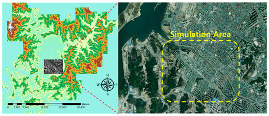
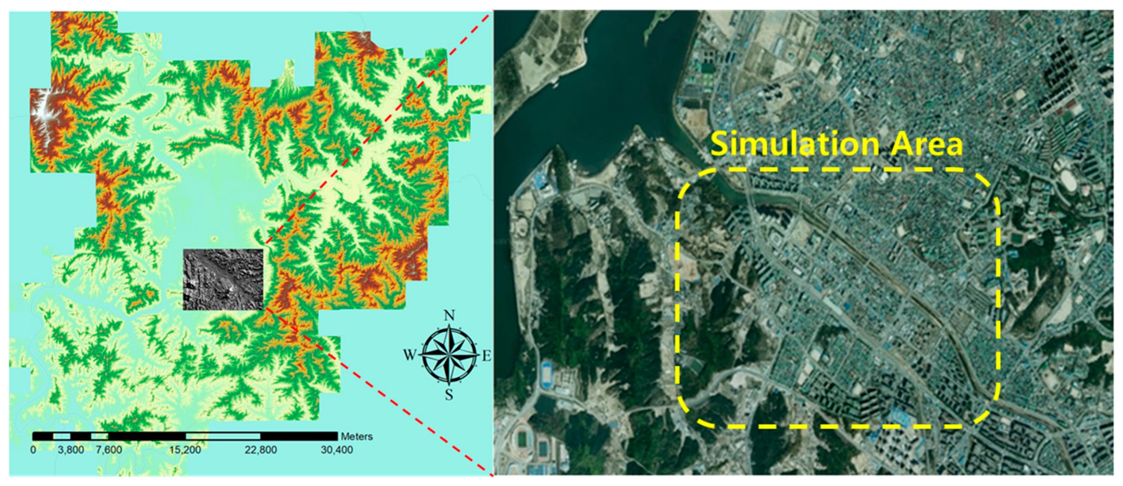
For this study, the Gongjicheon watershed in Chuncheon, located downstream of the Soyanggang Dam in the Bukhan River basin, was selected as the research area. Figure 1 shows the Location of map and Satellite image of study area. Although this watershed is not frequently affected by flooding under normal conditions, it includes extensive low-lying areas along the river corridor. During record-breaking heavy rainfall events combined with restricted discharge from the Soyanggang Dam, severe flooding occurred in residential districts and road networks. Most inundated areas were situated near levees, where stormwater drainage facilities became overwhelmed under intense rainfall, leading to rapid urban flooding and significant inundation damage in low-elevation residential areas.

Figure 1. Location map and satellite image of Study area in Chuncheon, Gangwon Province, Korea. The left map highlights the located downstream of the Soyanggang Dam in the Bukhan River basin. The right image provides a satellite view of the terrain and urban features around the target site.

Importantly, the Gongjicheon watershed exhibits key characteristics that are highly sensitive to DEM resolution effects in flood modeling, including complex local topography, mixed urban–agricultural land use, narrow channels, and artificial structures such as levees and road embankments. These features strongly influence flow routing and inundation patterns and are commonly observed in many Korean watersheds. Therefore, despite the relatively infrequent occurrence of flooding under average hydrologic conditions, the selected watershed is considered representative for evaluating the effects of DEM source and resolution on flood inundation simulation.

2.2. FLO-2D Simulation

The FLO-2D model is a physically based, finite-difference hydrodynamic model designed for flood hazard analysis. The computational domain is discretized into uniform, square grid cells, and surface runoff is routed in eight directions (N, S, E, W, NE, SE, NW, SW). Flow exchange between adjacent cells is solved at each time step using the governing continuity and momentum equations [17].

Governing Equations

The continuity equation is expressed as:

$${\displaystyle \frac{\partial h}{\partial t}}+{\displaystyle \frac{\partial h{V}_x}{\partial x}}=i$$

(1)

$$S_{fx}=S_{0x}-{\displaystyle \frac{\partial h}{\partial x}}-{\displaystyle \frac{V_x}{\partial x}}{\displaystyle \frac{\partial V_x}{\partial x}}-{\displaystyle \frac{V_x}{g}}{\displaystyle \frac{\partial V_x}{\partial x}}-{\displaystyle \frac{1}{g}}{\displaystyle \frac{\partial V_x}{\partial t}}$$

(2)

Here, h is the fluid depth (m), V is the mean velocity, i is the excess rainfall intensity, S_f is the friction slope velocity (Manning’s equation), and S₀ denotes the bed slope. The above equations represent the one-dimensional mean open-channel flow.

Although FLO-2D is a model capable of simulating multidirectional flow, the equation of motion in FLO-2D is applied to calculate the mean velocity across the grid boundary in a single direction. There are eight potential flow directions (east, west, south, north, northeast, southeast, northwest, southwest). The velocity in each direction is calculated in one dimension and is independent of the other seven directions. The friction slope is estimated using Manning’s equation:

$$S_f={\displaystyle \frac{n^2{V}^2}{h^{\raisebox{1ex}{$4$}\!\left/ \!\raisebox{-1ex}{$3$}\right.}}}$$

(3)

2.3. Model Application and Data Base Construction

This formulation allows FLO-2D to simulate overland flood propagation, channel routing, and floodplain storage with realistic flow interactions across multiple directions. For typical alluvial channels with moderate slopes, the dynamic wave approximation adequately reproduces flood wave propagation [17]. Inclusion of the pressure-gradient term also improves simulation accuracy in complex topography where floodplain storage and diffusion processes dominate.

The methods for constructing precise 3D terrain models are currently being implemented and utilized through various surveying techniques such as digital topographic maps, aerial photography, satellite imagery, and LiDAR. These surveying techniques should be selected appropriately based on the scale, characteristics, purpose, and required accuracy of the study area. In this study, LiDAR data covering the watershed contributing to flooding was acquired to construct a precise Digital Elevation Model (DEM) for flood inundation simulation.

To produce the DEM of the study area, point data obtained from the LiDAR system were interpolated at the required spatial resolution. Among commonly used interpolation techniques for LiDAR data, such as Natural Neighbor Interpolation and Kriging Interpolation, the Kriging Interpolation method was adopted in this study. In addition to the LiDAR-based DEM, a comparative DEM was generated from a 1:5000 topographic map, which has a grid resolution of 5 m.

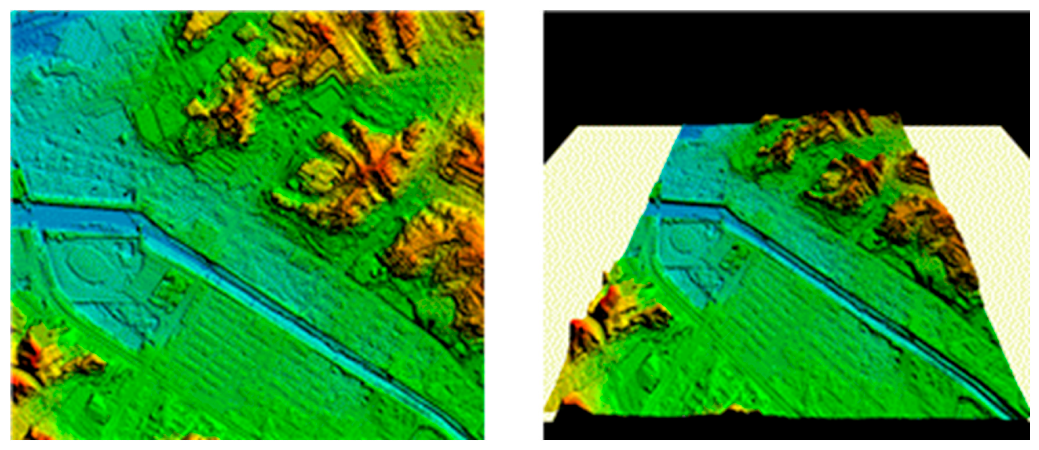
For the LiDAR-derived dataset, a Digital Surface Model (DSM) was first constructed through interpolation of the LiDAR point clouds. Based on this DSM, vegetation and artificial structures, including bridges, were removed to derive a DEM that accurately represents river flow conditions. This process involved the removal of both artificial structures and natural features, such as vegetation, using filtering methods incorporating mathematical functions. Figure 2 shows the results of removal process.

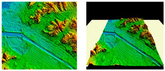
Figure 2. Visualization of the airborne LiDAR-derived DEM over the Gongjicheon area. Fine-scale topographic elements such as levees, drainage channels, and road networks are clearly distinguishable, enabling accurate hydrodynamic simulations.

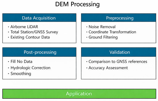
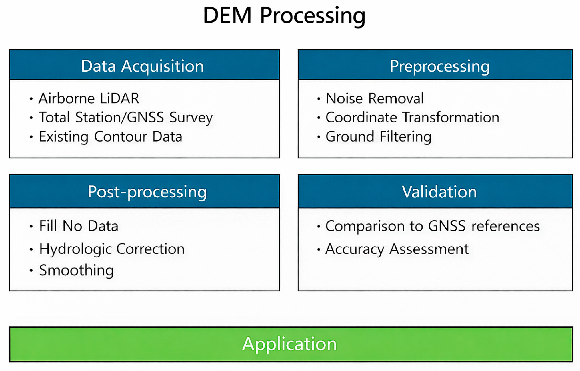
The LiDAR point clouds were further classified into ground and non-ground points (e.g., buildings and vegetation) using a progressive TIN densification filter. Non-ground features were eliminated, and only ground-classified points were interpolated to generate a Digital Terrain Model (DTM). The detailed workflow of DEM processing, including classification and filtering procedures, is illustrated in Figure 3.

Figure 3. Workflow of DEM processing, including data acquisition, preprocessing, post-processing, validation, and application.

3. Simulation and Analysis

3.1. Geospatial Data Resolution Comparison

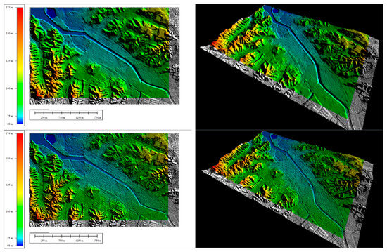
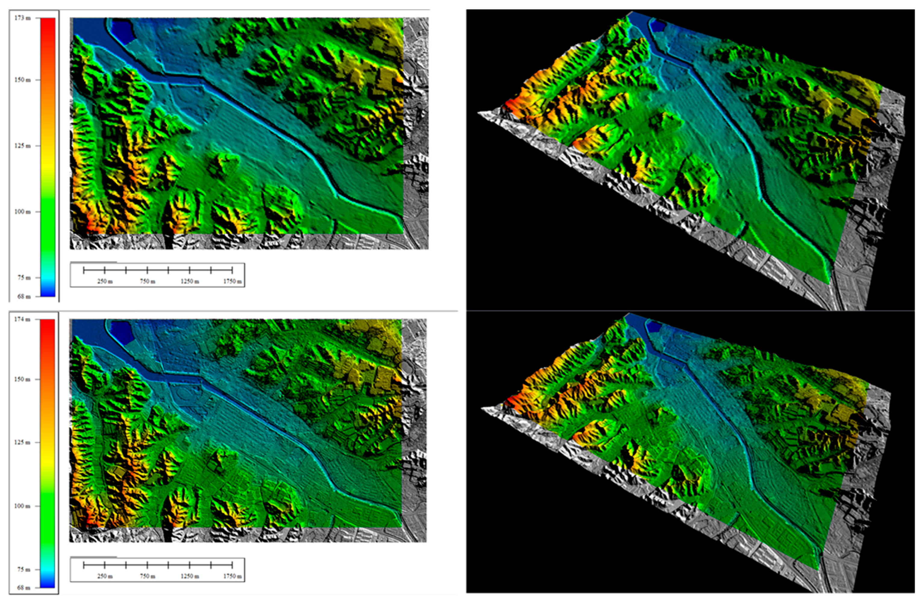
Accurate representation of terrain characteristics is a critical factor influencing the reliability of flood inundation modeling. Figure 4 compares DEMs generated from different data sources: a 1:5000 digital topographic map and LiDAR survey data with a 1 m spatial resolution. The top panels illustrate the DEM derived from the 1:5000 topographic map, which provides a generalized depiction of terrain but lacks the ability to capture small-scale topographic variations such as levees, drainage channels, and urban infrastructure. As a result, fine-scale hydrological features are often smoothed or omitted, limiting the precision of inundation simulations.

Figure 4. Comparison of terrain representation between the 1:5000 topographic map–derived DEM (upper panels) and the high-resolution LiDAR-derived DEM (lower panels). The left panels present shaded relief visualizations displayed at the original grid resolution, while the right panels show three-dimensional perspective views with color-coded elevation. The 1:5000 DEM exhibits generalized terrain morphology with smoothed river–valley features and limited representation of small-scale topographic elements. In contrast, the LiDAR-derived DEM clearly resolves fine-scale terrain characteristics, including levees, drainage channels, road embankments, and agricultural field boundaries. The improved legibility and consistent visualization parameters in the revised figure allow a clearer comparison of terrain resolution effects and highlight the advantages of high-resolution LiDAR data for detailed flood hazard modeling and spatial analysis.

In contrast, the bottom panels show the LiDAR-derived DEM, which clearly delineates micro-topographic features including secondary channels, road networks, and embankments. The improved resolution enhances the representation of watershed morphology and enables more accurate simulation of overland flow paths and flood extents. This comparison highlights the importance of using high-resolution terrain data in flood hazard analysis, as LiDAR DEMs provide the necessary level of detail for precise hydrodynamic modeling and risk mapping.

3.2. Simulation Analysis Procedure

FLO-2D has been extensively applied in urban flood simulations and has shown reliable performance in reproducing observed flood events [6,7,13,16,18]. In this study, the model was calibrated by adjusting the inflow boundary hydrograph, downstream water level boundary, and Manning’s roughness coefficient (n) to reflect urban surface resistance.

The calibration process aimed to ensure that the simulated inundation depth and extent were consistent with available historical flood information and local records. Final parameter values used in the simulation are summarized in Table 1.

Table 1. FLO-2D control variable settings used in this study. This panel shows the hydrodynamic simulation parameters applied to both the 1 m LiDAR DEM and the 1:5000 topographic map–derived DEM. All major model components—including rainfall input, infiltration, channel routing, surface detention, and numerical stability settings—were kept identical to ensure that differences in simulation results originated solely from the DEM resolution rather than model configuration.

Category	Variable/Option	Setting/Value	Description
Time Control	Simulation Time (h)	1	Total simulation duration
	Output Interval (h)	0.05	Output frequency in hours
	Graphics Display	Detailed Graphics	Enables visual output
Global Data Modification	n-value Adjustment	0	No change applied to Manning’s n
	Shallow Flow n-value	0.2	Manning’s n for shallow flows
System Component Switches	Main Channel	Enabled	Main drainage channel included
	Area Reduction Factors (ARF)	Enabled	Applies areal rainfall reduction
Physical Process Switches	Rainfall	Enabled	External rainfall input included
	Infiltration	Enabled	Infiltration process considered
Conveyance Structures	Hydraulic Structures/Debris Basin	Disabled	No artificial conveyance or basin included
	Floodway Analysis	Disabled	Not considered
Numerical Stability Parameters	Surface Detention (m)	0.03	Surface retention depth
	% Change in Flow Depth	0.2	Threshold for flow depth update
	Dynamic Wave Stability Coefficient	1	Governs wave stability
	Courant Number	0.6	For numerical stability (CFL condition)
Output Options	Floodplain Output	No Output	No floodplain file generated

As illustrated in Table 1, the FLO-2D control variables—such as rainfall forcing, infiltration options, main channel activation, numerical stability parameters (surface detention, Courant number), and global data modification settings—were identically applied across both DEM scenarios. This ensured that any differences in flood depth or velocity were attributable strictly to terrain resolution rather than model parameterization.

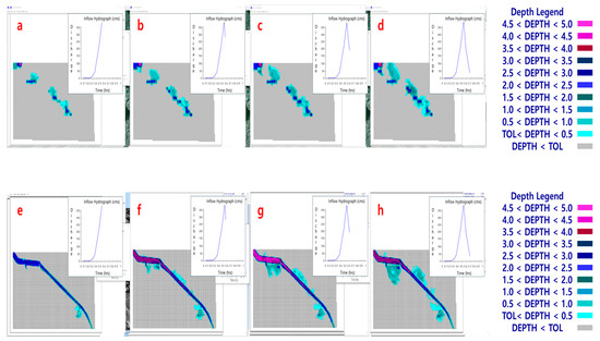
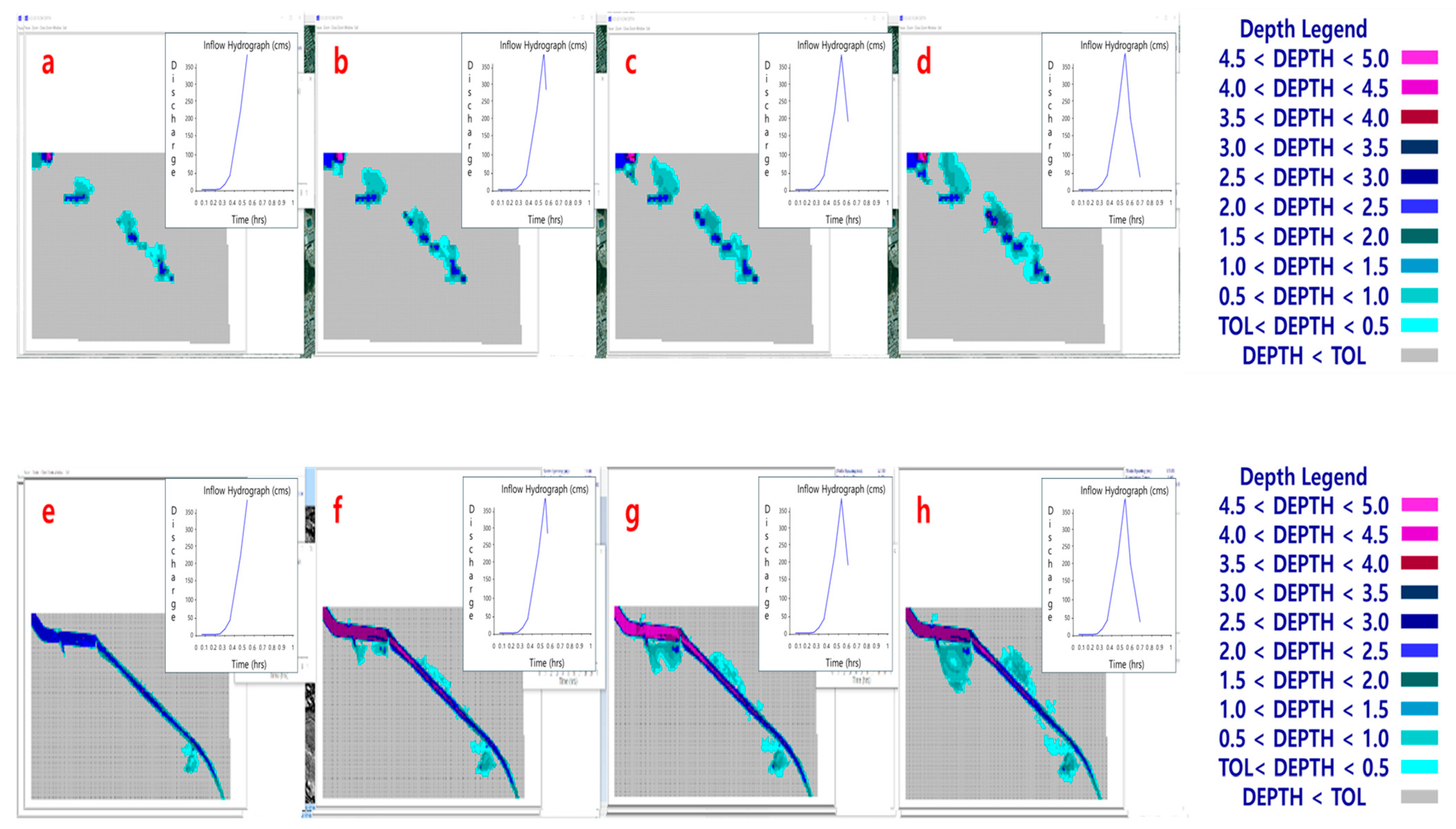
To examine the impact of terrain data resolution on flood simulation, FLO-2D was executed with identical boundary conditions and model parameters, while only the DEM input varied. Figure 5 shows the simulation analysis procedure and the temporal evolution of flood inundation under different DEM resolutions. Figure 5a–d represent sequential simulation snapshots using the 1:5000 topographic map-derived DEM, whereas Figure 5e–h correspond to results obtained from the LiDAR-derived DEM (1 m resolution). This design ensures that the differences observed in flood propagation are solely attributable to DEM resolution, providing an intuitive demonstration of how terrain detail influences the spatiotemporal dynamics of inundation.

Figure 5. FLO-2D simulation results comparing flood inundation patterns derived from different digital elevation model (DEM) sources. Panels (a–d) show the time-series inundation extent and water depth simulated using a 1:5000 topographic map-based DEM, while panels (e–h) illustrate results obtained from a LiDAR-derived DEM with 1 m resolution. Each sequence (a–h) represents the temporal progression of inundation under the same inflow hydrograph conditions, with color shading indicating water depth (m) according to the depth legend. The comparison highlights that the LiDAR-based DEM captures more detailed flow paths and flood extents, whereas the 1:5000 DEM provides a generalized representation with limited terrain resolution.

3.3. Simulation Results

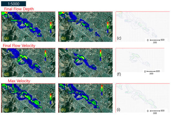
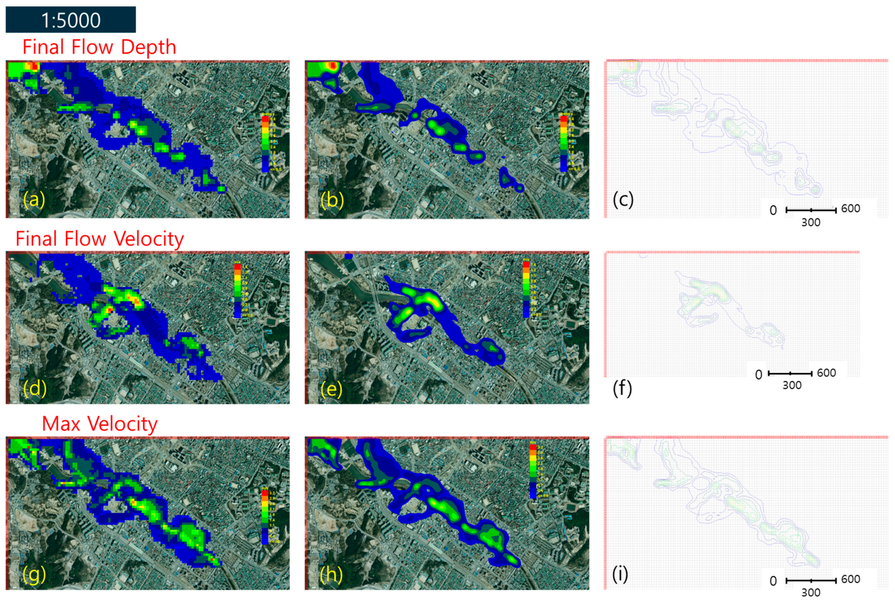
Figure 6 presents the spatial distribution of final flow depth, final flow velocity, and maximum flow velocity simulated with two different DEM resolutions: a 1:5000 topographic map-derived DEM and a LiDAR-derived DEM with 1 m resolution.

Figure 6. Visualization of flood simulation results using the 1:5000-scale topographic DEM. (a,d,g) Grid-based representation directly showing the original computational cell outputs; (b,e,h) Shaded-contour rendering for enhanced visual continuity and smoother inundation gradients; (c,f,i) Contour-line visualization highlighting the spatial variation in water-surface elevation and velocity gradients.

In the case of the 1:5000 DEM, the inundation extent appeared more fragmented and generalized. Final flow depth was unevenly distributed, and localized flood pathways were not clearly represented. Similarly, the velocity fields were simplified, with maximum flow velocity underestimated in areas where small drainage channels or low-lying depressions were absent from the coarse terrain representation. As a result, the simulation tended to smooth hydrodynamic variability, limiting its applicability for detailed flood risk mapping.

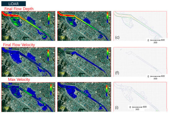
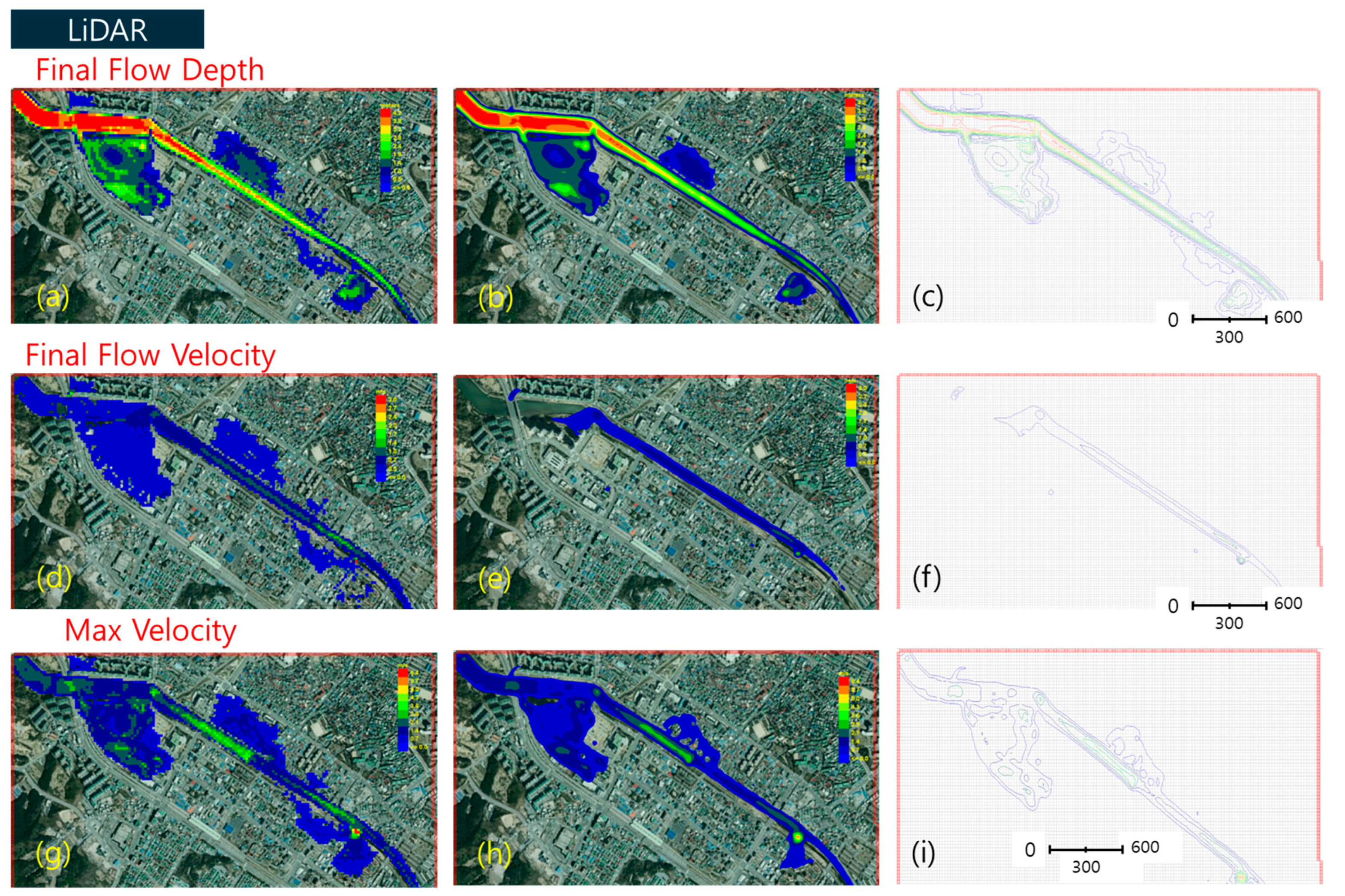
Figure 7 compares three visualization approaches applied to the 1 m LiDAR DEM-based simulation results.

Figure 7. Flood simulation results based on the 1 m LiDAR-derived DEM. (a,d,g) Grid-based representation directly showing the original computational cell outputs; (b,e,h) Shaded-contour rendering for enhanced visual continuity and smoother inundation gradients; (c,f,i) Contour-line visualization highlighting the spatial variation in water-surface elevation and velocity gradients.

Compared with the 1:5000-scale DEM results, the 1 m LiDAR DEM provides sharper and more realistic depiction of local flow concentration and micro-topographic effects, improving the interpretation of urban flood behavior.

By contrast, the LiDAR DEM provided a significantly more detailed and realistic representation of flood dynamics. The final flow depth map captured continuous inundation zones, especially along secondary channels and low-lying areas that were omitted in the 1:5000 DEM. Both final and maximum velocity maps showed higher values and clearer spatial variability, reflecting the influence of fine-scale topographic features such as levees, embankments, and urban infrastructure. These results highlight the importance of terrain resolution in accurately predicting flow concentration zones and high-velocity pathways, which are critical for assessing flood hazards to infrastructure and communities.

Overall, the comparison confirms that LiDAR-derived DEMs improve the reliability of flood simulations by providing more precise hydrodynamic outputs. While 1:5000 DEMs may suffice for broad-scale assessments, their limitations in representing micro-topography can lead to underestimation of inundation extent and flow hazards at the local scale.

3.4. Raster Data Analysis

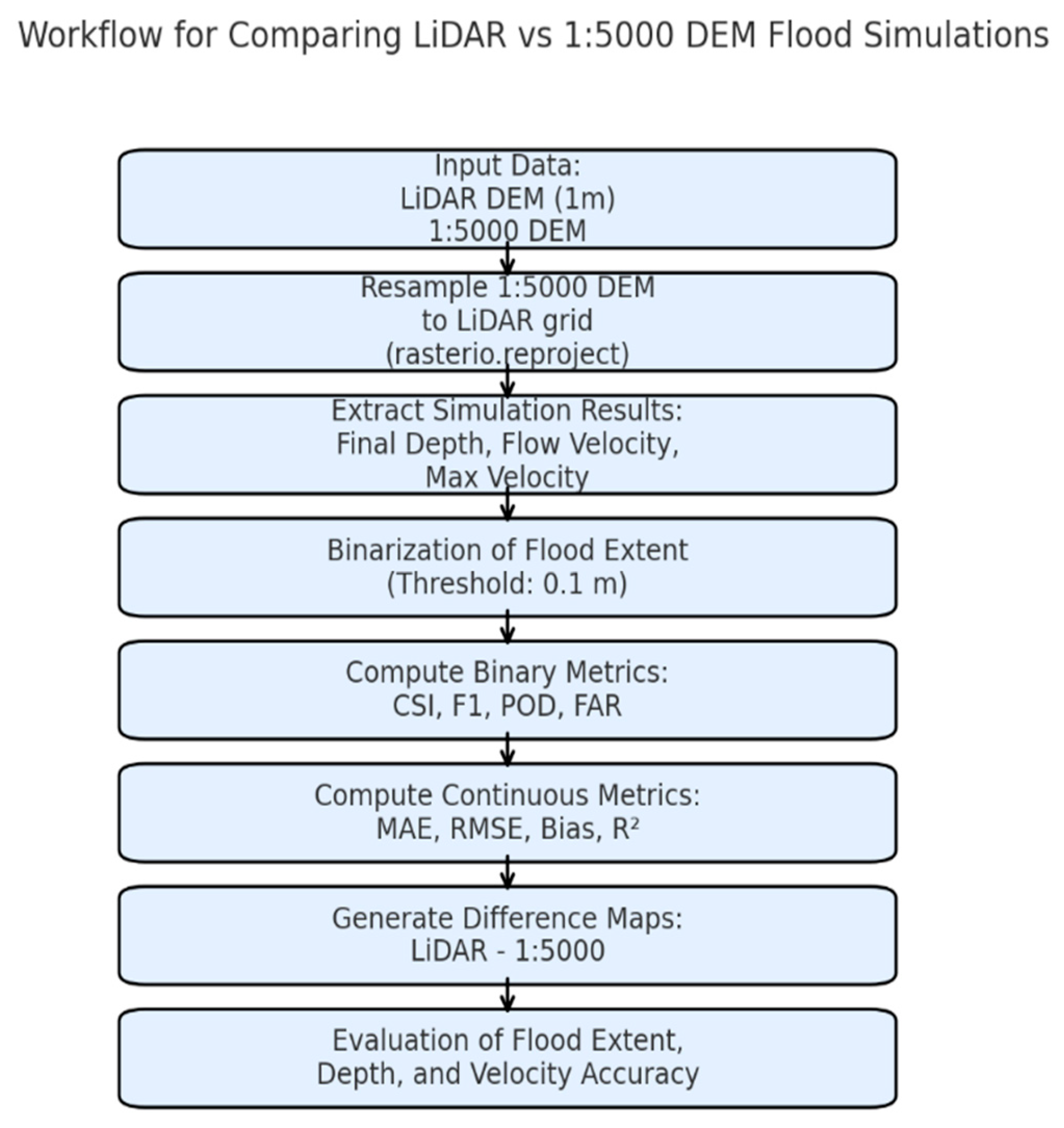
To quantitatively assess the impact of topographic resolution on flood simulation outputs, we implemented a raster-based comparison workflow using the rasterio library in Python (ver 3.12.12). The analysis was performed on two datasets: flood simulation results derived from a 1 m resolution LiDAR DEM and those based on a DEM generated from a 1:5000 topographic map.

First, the DEM products were spatially aligned by resampling the coarser 1:5000 DEM to match the resolution, extent, and coordinate reference system of the LiDAR DEM using bilinear interpolation. This preprocessing step ensured pixel-to-pixel comparability between the two datasets. Subsequently, raster values representing simulation outputs—including final flood depth, flow velocity, and maximum velocity—were extracted from both DEM-based simulations.

To evaluate the similarity of flood extent, each raster was binarized using a 0.1 m inundation-depth threshold. This threshold was selected following common practice in flood hazard mapping and two-dimensional hydrodynamic modeling, where shallow water depths below 0.1 m are often considered negligible in terms of damage potential and flow continuity and are frequently used as minimum wet/dry or inundation criteria. Applying this threshold also helps to reduce numerical noise and to delineate meaningful inundation extents. Based on the binarized rasters, binary classification statistics—including the Critical Success Index (CSI), F1-score, Probability of Detection (POD), and False Alarm Ratio (FAR)—were derived from confusion matrices.

In addition, continuous statistical measures—Mean Absolute Error (MAE), Root Mean Square Error (RMSE), Bias, and the coefficient of determination (R²)—were computed for pixels classified as inundated in at least one of the two datasets. Finally, spatial difference maps were generated by subtracting the 1:5000 DEM-based results from the LiDAR DEM-based results. These visualizations provide an intuitive representation of localized discrepancies, highlighting areas of overestimation and underestimation attributable to differences in DEM resolution.

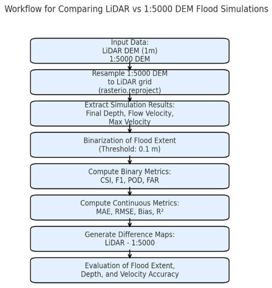
Figure 8 shows workflow enabled both categorical and continuous evaluation of model performance, offering a systematic means to quantify the degree to which terrain resolution affects simulated flood extents, depths, and velocities.

Figure 8. Schematic workflow illustrating the comparison of flood simulation outputs between high-resolution LiDAR and 1:5000 DEMs using statistical and spatial analysis methods.

3.5. Comparison Results Analysis

The evaluation metrics in Table 2 reveal clear resolution-dependent differences between the LiDAR-based and 1:5000 DEM simulations. The binary agreement indicators—namely the critical success index (CSI), F1 score, probability of detection (POD), and false alarm ratio (FAR)—suggest that the 1:5000 DEM is generally capable of delineating the broad extent of inundation. This is particularly evident for flow velocity, where CSI (0.966), F1 (0.983), and POD (1.000) are high, and FAR remains low (0.034), indicating minimal overprediction.

Table 2. Summary of binary agreement and continuous statistical metrics comparing flood simulation results derived from LiDAR and 1:5000 DEMs. The metrics were calculated for three key variables: final flow depth, flow velocity, and maximum flow velocity. Binary metrics (CSI, F1, POD, FAR) evaluate the spatial agreement in flood extent classification, while continuous metrics (MAE, RMSE, Bias, R²) quantify the magnitude and direction of discrepancies across the flood simulation outputs.

	Binary Agreement Metrics				Continuous Metrics
	CSI	F1	POD	FAR	MAE	RMSE	Bias	R2
Final Flow Depth (cm)	0.707	0.829	0.720	0.023	56.893	76.382	−26.939	−1.2
Flow Velocity (m/s)	0.966	0.983	1.000	0.034	43.248	58.007	−3.279	0.01
Maximum Velocity (m/s)	0.734	0.846	0.765	0.054	53.049	68.435	−17.269	−1.314

However, the continuous error metrics provide a more detailed picture of the quantitative discrepancies introduced by the coarser terrain data. For final flow depth, the mean absolute error reaches 56.893 cm and the root mean square error exceeds 0.76 m, accompanied by a substantial negative bias (−26.939 cm), indicating systematic underestimation of water depth. Maximum flow velocity shows a comparable pattern, with an RMSE of 0.68 m/s and a negative bias of −0.17 m/s, reflecting the inability of the 1:5000 DEM to adequately represent localized high-velocity zones such as constricted channels or roadway embankments. Although overall flow velocity exhibits better agreement in magnitude (RMSE = 0.58 m/s), the low coefficient of determination (R² = 0.01) highlights weak linear consistency between the two DEM-driven simulations. It should be emphasized that R² is used here solely as a metric for inter-model comparison to quantify systematic differences between simulations driven by different DEM sources, rather than as a measure of absolute model validation against independent observations.

Taken together, these results demonstrate that while medium-resolution DEMs may suffice for coarse-scale inundation mapping, they are insufficient for producing reliable quantitative estimates of flood depth and velocity. The errors observed here originate primarily from the loss of micro-topographic detail—such as levees, drainage pathways, and embankments—which exert strong control on localized hydraulic behavior. Consequently, high-resolution LiDAR DEMs are essential for hydrodynamic modeling in urbanized or infrastructure-sensitive settings, where small-scale variations directly influence hazard assessment and risk-informed decision-making.

4. Discussion

This study investigated the influence of terrain data resolution on hydrodynamic model behavior by comparing a high-resolution 1 m LiDAR DEM with a DEM derived from a 1:5000 topographic map. It is important to emphasize that the primary objective of this analysis was not absolute validation against independent flood observations, but rather a comparative assessment of DEM-induced sensitivities and relative differences between model simulations. Such an approach is commonly adopted in DEM resolution studies when spatially comprehensive observational datasets (e.g., distributed high-water marks or velocity measurements) are unavailable, particularly in urban and small mountainous watersheds.

Within this comparative framework, and consistent with previous studies highlighting the strong dependence of flood model outputs on terrain representation [19,20], the binary agreement metrics indicate that the 1:5000 DEM is capable of reproducing the general inundation extent (e.g., CSI = 0.707, F1 = 0.829). However, the continuous evaluation metrics reveal substantial quantitative discrepancies that would be masked if only binary measures were considered. For final flood depth, the MAE (56.893 cm) and RMSE (76.382 cm), together with a pronounced negative bias (−26.939 cm), indicate systematic underestimation associated with the coarser DEM. Similar degradation patterns have been widely reported in flood and debris-flow studies, where coarse grids smooth micro-topography and distort hydraulic gradients, channel confinement, and flow depths [21,22,23].

Comparable discrepancies were observed for flow velocity and maximum velocity, with RMSE values of 58.007 cm/s and 68.435 cm/s, respectively. These results reinforce findings from both flood and debris-flow applications of FLO-2D, which consistently demonstrate that velocity-related variables are particularly sensitive to terrain resolution because they directly depend on slope continuity, channel geometry, and local roughness representation [24,25]. The relatively weak coefficients of determination (R² = 0.01 for flow velocity and negative values for depth) should therefore not be interpreted as indicators of poor model performance in an absolute sense. Rather, they reflect systematic divergence between simulations driven by different DEM sources, highlighting the limits of inter-model agreement when terrain resolution differs substantially. Similar interpretations have been reported in coupled surface–subsurface flood modeling studies, where fine-scale terrain representation is essential for capturing hydraulic thresholds and transition zones [26].

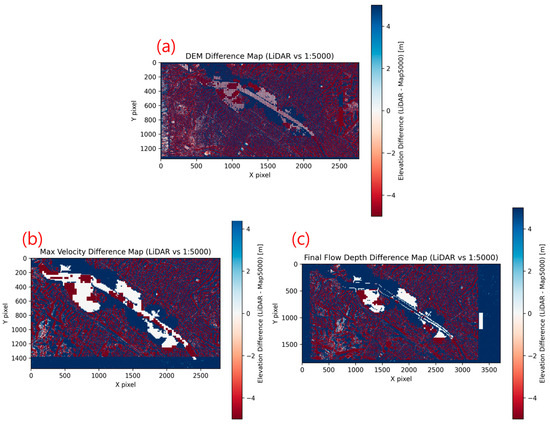
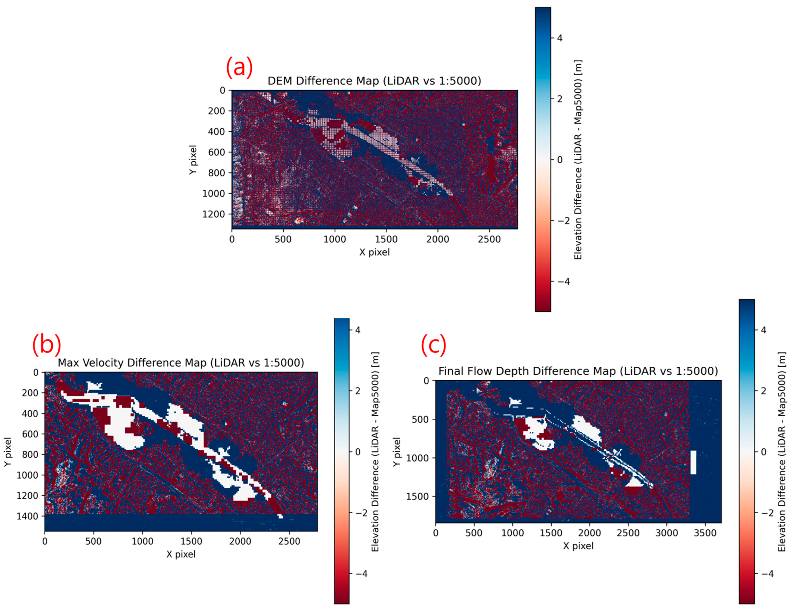
Difference maps (Figure 9) further reveal localized elevation mismatches of approximately ±3–4 m around levees, drainage pathways, and road embankments. These discrepancies are not random, but spatially clustered at geomorphically and infrastructurally critical locations. Comparable patterns have been documented in arid-valley hazard assessments [27], large-scale flood exposure studies [28], and DEM-fusion frameworks [29], all of which emphasize that terrain-induced errors are amplified at locations where flow routing is strongly constrained. Such effects are especially pronounced in compact watersheds and rapidly urbanizing areas, such as the Gongjicheon basin, where artificial structures exert a dominant control on inundation mechanisms [30,31].

Figure 9. Spatial difference maps comparing LiDAR-derived and 1:5000 DEM-based flood simulation results. (a) Digital Elevation Model (DEM) difference map showing elevation discrepancies between LiDAR and 1:5000 sources. (b) Maximum flow velocity difference map highlighting regions with significant deviations in peak velocities. (c) Final flow depth difference map illustrating variations in simulated floodwater depths. All difference values are presented in meters, with blue indicating areas where LiDAR estimates are lower and red indicating higher values compared to the 1:5000 DEM.

Several limitations of the present study should be acknowledged. First, the analysis was conducted for a single rainfall scenario, and sensitivity to different rainfall return periods was not explicitly examined. The magnitude of DEM-resolution effects may vary under more extreme or prolonged flood events, and future studies should extend the analysis to multiple design storms to better characterize nonlinear interactions between rainfall intensity and terrain representation. Second, the case-study nature of the analysis limits direct generalization to other geomorphic settings, such as extremely flat floodplains or large alluvial rivers. Nonetheless, the observed error magnitudes and spatial patterns are consistent with international findings, suggesting that the qualitative implications are transferable to similar urban or mountain-adjacent catchments.

Despite these limitations, the results reinforce extensive international evidence that while medium-resolution DEMs may be adequate for screening-level or reconnaissance flood mapping, they lack the fidelity required for engineering-grade assessments, infrastructure design evaluation, and velocity-sensitive hazard analysis [32]. High-resolution LiDAR DEMs have repeatedly been shown to improve floodplain delineation, micro-topographic detection, and hydrodynamic accuracy—particularly in urban environments where road networks, levees, and drainage structures exert strong controls on flow patterns [19,22,23].

From a methodological perspective, the Python-based rasterio workflow adopted in this study enabled pixel-level comparison and explicit quantification of DEM-induced error propagation. Similar computational frameworks have been successfully applied in rapid inundation modeling and hybrid machine-learning approaches to flood prediction [33], supporting the robustness and reproducibility of the proposed analysis framework for high-resolution flood risk assessment.

Finally, the comparison of computational efficiency across 0.5 m, 1 m, and 5 m DEMs highlights an important practical consideration. The 1 m DEM achieved accuracy comparable to the 0.5 m DEM while requiring only approximately one-third of the computational resources. This finding aligns with recent studies showing diminishing accuracy gains at sub-meter resolutions when computational cost is considered [21,23]. Accordingly, the results confirm that 1 m LiDAR DEMs provide an optimal balance between accuracy and efficiency for operational flood modeling and near-real-time hazard assessment in steep or urbanized catchments (Table 3).

Table 3. 1 m LiDAR DEMs provide an optimal balance between accuracy and efficiency.

DEM Resolution	Average Runtime (min)	Peak Memory Usage (GB)	Flood Depth RMSE (cm)	Remarks
5 m	14	2.1	0.186	Coarse terrain; underestimation of flood extent
1 m	68	7.8	0.082	Balanced accuracy and computational cost
0.5 m	215	18.4	0.076	High computational cost; minor improvement in accuracy

5. Conclusions

This study demonstrates that coarse 1:5000 DEMs can approximate the broad spatial extent of flooding but introduce substantial quantitative errors in flood depth and velocity. The occurrence of negative or near-zero R² values, together with elevated MAE and RMSE, indicates that fine-scale hydraulic variability and micro-topographic controls are not adequately captured at this resolution. In contrast, high-resolution LiDAR DEMs provide a more faithful representation of micro-topographic features and urban infrastructure, resulting in more reliable hydrodynamic simulation outcomes.

It is important to emphasize that the proposed analysis framework is primarily intended for screening-level and comparative assessments, where the objective is to evaluate the relative sensitivity of flood model outputs to DEM source and resolution rather than to achieve absolute agreement with observed flood conditions. Within this context, the results clearly support the use of LiDAR-based terrain data for quantitative flood hazard analysis and risk-informed decision-making, particularly in dense urban or infrastructure-sensitive environments. Conversely, 1:5000 DEMs may be considered suitable for preliminary screening or reconnaissance-level applications, where detailed quantitative accuracy is not critical.

For engineering-grade flood analysis, which requires rigorous calibration and validation against independent observations, additional data, event-based testing, and site-specific parameter optimization are necessary. Future work should therefore extend the proposed framework to multiple flood events and diverse physiographic settings, evaluate cost–benefit trade-offs associated with LiDAR acquisition, and explore DEM fusion strategies (e.g., combining LiDAR with photogrammetric or UAV-derived data) to balance spatial coverage and accuracy. The integration of reproducible, open workflows (e.g., Python/rasterio) into operational practice is also recommended to standardize DEM resolution sensitivity checks and enhance transparency in flood hazard assessments.

References

- Hsu, Y.-C.; Prinsen, G.; Bouaziz, L.; Lin, Y.-J.; Dahm, R. An Investigation of DEM Resolution Influence on Flood Inundation Simulation. Procedia Eng. 2016, 154, 826–834. [Google Scholar] [CrossRef] [Scilit]
- Barbaro, G.; Bombino, G.; Foti, G.; Barillà, G.C.; Puntorieri, P.; Mancuso, P. Possible Increases in Floodable Areas Due to Climate Change: The Case Study of Calabria (Italy). Water 2022, 14, 2240. [Google Scholar] [CrossRef] [Scilit]
- Zhu, H.; Chen, Y. A Study of the Effect of DEM Spatial Resolution on Flood Simulation Accuracy. Remote Sens. 2024, 16, 3105. [Google Scholar] [CrossRef] [Scilit]
- Wang, H.V.; Loftis, J.D.; Liu, Z.; Forrest, D.; Zhang, J. The Storm Surge and Sub-Grid Inundation Modeling in New York City during Hurricane Sandy. J. Mar. Sci. Eng. 2014, 2, 226–246. [Google Scholar] [CrossRef] [Scilit]
- Zhang, Y. Using LiDAR-DEM Based Rapid Flood Inundation Modelling Framework to Map Floodplain Inundation Extent and Depth. J. Geogr. Sci. 2020, 30, 1649–1663. [Google Scholar] [CrossRef] [Scilit]
- Shen, D.; Wang, J.; Cheng, X.; Rui, Y.; Ye, S. Integration of 2-D hydraulic model and high-resolution lidar-derived DEM for floodplain flow modeling. Hydrol. Earth Syst. Sci. 2015, 19, 3605–3616. [Google Scholar] [CrossRef] [Scilit]
- Rodríguez, R.; Robles-Morua, A.; Meza-Figueroa, D.; Tuxpan-Vargas, J.; Cisneros Almazán, R.; Perez Ramos, N.; Sen-Gupta, B.; Martínez-Villegas, N. Urban Flood Exposure Assessment Through Citizen Science, 2D Hydraulic Modeling, and Artificial Intelligence. J. Environ. Manag. 2025, 393, 127037. [Google Scholar] [CrossRef] [Scilit] [PubMed]
- Muhadi, N.A.; Abdullah, A.F.; Bejo, S.K.; Mahadi, M.R.; Mijic, A. The Use of LiDAR-Derived DEM in Flood Applications: A Review. Remote Sens. 2020, 12, 2308. [Google Scholar] [CrossRef] [Scilit]
- Fereshtehpour, M.; Esmaeilzadeh, M.; Alipour, R.S.; Burian, S.J. Impacts of DEM Type and Resolution on Deep Learning-Based Flood Inundation Mapping. arXiv 2023, arXiv:2309.13360. [Google Scholar] [CrossRef] [Scilit]
- Aristizabal, F.; Sampson, C.; Neal, J.; Brown, J.D. Effects of High-Quality Elevation Data and Explanatory Variables on the Accuracy of Flood Inundation Mapping via Height Above Nearest Drainage (HAND). Hydrol. Earth Syst. Sci. 2024, 28, 1287–1304. [Google Scholar] [CrossRef] [Scilit]
- Bryant, S.; Neal, J.; Savage, J.; Wing, O.; Sampson, C.; O’Loughlin, F.; Bates, P. Resolution Enhancement of Flood Inundation Grids Using a Downscaling Approach. Hydrol. Earth Syst. Sci. 2024, 28, 575–595. [Google Scholar] [CrossRef] [Scilit]
- Liu, Y.; Zhang, Y.; Zhang, J.; Zhao, T.; Sun, W. Bare-Earth DEM Generation from ArcticDEM and Its Use in Flood Simulation. Nat. Hazards Earth Syst. Sci. 2023, 23, 375–391. [Google Scholar] [CrossRef] [Scilit]
- Erena, S.H.; Worku, H.; De Paola, F. Flood Hazard Mapping Using FLO-2D and Local Management Strategies of Dire Dawa City, Ethiopia. J. Hydrol. Reg. Stud. 2018, 19, 224–239. [Google Scholar] [CrossRef] [Scilit]
- Peng, S.-H.; Lu, S.-C. FLO-2D simulation of mudflow caused by large landslide due to extremely heavy rainfall in southeastern Taiwan during Typhoon Morakot. J. Mt. Sci. 2013, 10, 207–218. [Google Scholar] [CrossRef] [Scilit]
- Adegbe, M.; Alkema, D.; Jetten, V.G.; Agbor, A.T.; Abdullahi, I.N.; Shehu, O.U.; Unubi, A.S. Post-seismic debris flow modelling using FLO-2D: Case study of Yingxiu, Sichuan Province, China. J. Geogr. Geol. 2013, 5, 101–115. [Google Scholar] [CrossRef] [Scilit]
- AL-Areeq, A.M.; Sharif, H.O.; Abba, S.I.; Chowdhury, S.; Al-Suwaiyan, M.; Benaafi, M.; Yassin, M.A.; Aljundi, I.H. Digital Elevation Model for Flood Hazards Analysis in Complex Terrain: Case Study from Jeddah, Saudi Arabia. Int. J. Appl. Earth Obs. Geoinf. 2023, 119, 103330. [Google Scholar] [CrossRef] [Scilit]
- FLO-2D Software, Inc. FLO-2D Model Validation Report for FEMA (Versions 2009 and Up); Technical Report; FLO-2D Software, Inc.: Nutrioso, AZ, USA, 2011; Available online: https://www.scribd.com/document/332298997/FLO-2D-Model-Validation (accessed on 8 January 2026).
- U.S. Army Corps of Engineers (USACE). Middle Rio Grande FLO-2D Model Development: Existing Conditions Report (Cochiti Dam to Elephant Butte Reservoir); Albuquerque District: Albuquerque, NM, USA, 2007; Available online: https://www.spa.usace.army.mil/Portals/16/docs/environmental/fonsi/App%20A_H&H%20Main%20report.pdf (accessed on 8 January 2026).
- Xu, K.; Fang, J.; Fang, Y.; Sun, Q.; Wu, C. The Importance of Digital Elevation Model Selection in Flood Simulation and a Proposed Method to Reduce DEM Errors: A Case Study in Shanghai. Int. J. Disaster. Risk Sci. 2021, 12, 890–902. [Google Scholar] [CrossRef] [Scilit]
- Xafoulis, N.; Tsekouras, G.; Panagopoulos, A.; Papaioannou, G. Evaluation of Various Resolution DEMs in Flood Risk Assessment and Practical Rules for Flood Mapping in Data-Scarce Geospatial Areas: A Case Study in Thessaly, Greece. Hydrology 2023, 10, 91. [Google Scholar] [CrossRef] [Scilit]
- Fereshtehpour, M.; Karamouz, M. DEM Resolution Effects on Coastal Flood Vulnerability Assessment: Deterministic and Probabilistic Approach. Water Resour. Res. 2018, 54, 4965–4982. [Google Scholar] [CrossRef] [Scilit]
- Jiang, Z.; Sainju, A.M. A Hidden Markov Tree Model for Flood Extent Mapping in Heavily Vegetated Areas Based on High Resolution Aerial Imagery and DEM: A Case Study on Hurricane Matthew Floods. Int. J. Remote Sens. 2021, 43, 1160–1179. [Google Scholar] [CrossRef] [Scilit]
- Tan, W.; Qin, N.; Zheng, Y.; Wang, C.; Li, Y. A Rapid High-Resolution Multi-Sensory Urban Flood Mapping Framework via DEM Upscaling. Remote Sens. Environ. 2024, 301, 113956. [Google Scholar] [CrossRef] [Scilit]
- Jia, X.; Wang, J.; Luo, Y.; Fan, H. Simulation and Management Impact Evaluation of Debris Flow in Dashiling Gully Based on FLO-2D Modeling. Appl. Sci. 2024, 14, 4216. [Google Scholar] [CrossRef] [Scilit]
- D’Agostino, V.; Tecca, P.R. Some considerations on the application of the FLO-2D model for debris flow hazard assessment. WIT Trans. Ecol. Environ. 2006, 90, 12. [Google Scholar] [CrossRef] [Scilit]
- Peña, F.; Nardi, F.; Melesse, A.; Obeysekera, J.; Castelli, F.; Price, R.M.; Crowl, T.; Gonzalez-Ramirez, N. Compound Flood Modeling Framework for Surface–Subsurface Water Interactions Using FLO-2D and MODFLOW-2005. Nat. Hazards Earth Syst. Sci. 2022, 22, 775–793. [Google Scholar] [CrossRef] [Scilit]
- Zhang, P.; Wang, Y.; He, H.; Chen, S. Hazard assessment of debris flow by using FLO-2D and hazard matrix: A case study of Qingshui Gully in the southern Gansu Province, China. Desalination Water Treat. 2023, 315, 650–662. [Google Scholar] [CrossRef] [Scilit]
- Ziwei, L.; Xiang, W.; Yaolin, Z.; Yang, L.; Tianzhu, G. GIS-Based Risk Assessment of Flood Disaster in the Lijiang River Basin. Sci. Rep. 2023, 13, 12890. [Google Scholar] [CrossRef] [Scilit]
- Abily, M.; Bertrand, N.; Delestre, O.; Gourbesville, P.; Duluc, C.-M. Global Sensitivity Analysis of High Resolution Classified Topographic Data Use in 2D Urban Flood Modelling. arXiv 2016, arXiv:1603.07279v1. [Google Scholar] [CrossRef] [Scilit]
- Mustafa, A.; Saeed, M.; Karim, M.; Sherwani, A.; Al-Bilali, H. GIS-Based Hydrodynamic Modeling for Urban Flood Mitigation in Fast-Growing Regions: A Case Study of Erbil, Kurdistan Region of Iraq. Sci. Rep. 2023, 13, 9786. [Google Scholar] [CrossRef] [Scilit]
- Kocsis, I.; Grigorescu, I.; Mirea, G. Flash Flood Vulnerability Mapping Based on FFPI Using the Valea Rea Catchment, Romania. Sensors 2022, 22, 3573. [Google Scholar] [CrossRef] [Scilit]
- Mayomi, I.; M.S., K.; Martins, A.K. Terrain Analysis for Flood Disaster Vulnerability Assessment: A Case Study of Niger State, Nigeria. Am. J. Geogr. Inf. Syst. 2014, 3, 122–134. [Google Scholar] [CrossRef]
- Bao, Y.; Mohammadpour Velni, J. A Hybrid Neural Network Approach for Adaptive Scenario-Based Model Predictive Control in the LPV Framework. IEEE Control Syst. Lett. 2023, 7, 1921–1926. [Google Scholar] [CrossRef] [Scilit]
Disclaimer/Publisher’s Note: The statements, opinions and data contained in all publications are solely those of the individual author(s) and contributor(s) and not of MDPI and/or the editor(s). MDPI and/or the editor(s) disclaim responsibility for any injury to people or property resulting from any ideas, methods, instructions or products referred to in the content. |
© 2026 by the authors. Licensee MDPI, Basel, Switzerland. This article is an open access article distributed under the terms and conditions of the Creative Commons Attribution (CC BY) license.