


Abstract
Transient mechanisms are increasingly applied in fields such as high-speed aircraft, super high-speed trains, and underwater robots. However, in high-speed motion, large inertial forces are inevitably generated, which can easily lead to elastic deformations in some flexible components of high-speed mechanisms, thereby affecting the performance of the mechanical system. To address this issue, this paper focuses on a transient unfolding mechanism driven by a high-speed actuator with flexible leading-edge rods. A rigid-flexible coupling dynamic model of the transient unfolding mechanism is established using the Absolute Nodal Coordinate Formulation (ANCF), and the theoretical model is validated by comparison with simulation models. The impact of flexible rods on the mechanism’s motion characteristics is studied, analyzing the effects of different deployment times, mechanism parameters, and rod materials on the mechanism’s dynamic properties. Based on this, four classical impact signals are chosen as input conditions to analyze the transient response characteristics of the mechanism under different input conditions. The dynamic characteristics of the transient mechanism are explained from an energy transfer perspective. Finally, a prototype of the transient unfolding mechanism is developed, and transient deployment tests are conducted. The test results verify the accuracy of the rigid-flexible coupling model established in this paper. The research findings provide valuable insights and guidance for the study and application of transient mechanisms.
1. Introduction
With the continuous advancements in modern aerospace, ultra-high-speed rail transportation, and robotics, the functional mechanisms required in these fields are evolving towards higher speeds, greater precision, and higher load-bearing capacities [1,2,3,4]. Taking the morphing aircraft, a research hotspot in the aerospace field, as an example, the requirements for the lift surface area, planar shape, and airfoil shape of an aircraft differ significantly across various speed regimes and airspace conditions. Morphing aircraft can actively adjust their shape to adapt to different flight missions [5,6,7,8]. Compared to fixed aircraft, morphing aircraft offer greater advantages in flight efficiency, environmental adaptability, and maneuverability. The mechanisms inside the wings of morphing aircraft need to be designed with lightweight, high-strength materials and must be capable of rapidly completing morphing functions such as flipping, extending, or changing sweep angles within sub-second timescales during high-speed flight while overcoming external aerodynamic loads. Traditional mechanisms can no longer meet the performance requirements for high speed, transient, complex, and heavy-load conditions, which has led to the emergence of new transient mechanisms that are being widely applied. The advent of transient mechanisms also presents new challenges for mechanical designers, as internal mechanisms of morphing aircraft are prone to strength failure or joint jamming issues when deployed or deformed under high overload conditions. Furthermore, transient mechanisms applied to morphing aircraft must not only possess high strength and rigidity but also meet the requirements for lightweight design and maneuverability. Compared to traditional mechanisms, transient mechanisms exhibit higher startup acceleration and operating speeds, and the enormous inertial forces generated during high-speed motion cannot be overlooked. Therefore, establishing accurate dynamic models of transient mechanisms and studying their transient dynamic characteristics is crucial for the design of these mechanisms. Apart from the aerospace field, the influence of high inertial forces on flexible components is also of broad research interest in industrial rotating systems. In industrial scenarios such as large turbomachinery, high-speed drive shafts and couplings, very high rotational inertial forces often induce significant elastic deformation of shaft systems, which in turn can trigger complex nonlinear vibrations and fatigue problems. The analysis method proposed here for the transient dynamics of flexible rods not only addresses high-speed morphing issues in aircraft but also provides valuable guidance for understanding and optimizing the transient response of industrial rotating systems during startup or speed variation and for improving the structural reliability of high-speed shaft systems [9,10].
In the field of rigid–flexible coupled mechanism modeling, Shabana proposed the ANCF based on the finite element method and continuum mechanics. In this formulation, the absolute nodal coordinates of each element are defined in the inertial coordinate system, and slope vectors are used to replace the conventional nodal rotation coordinates in traditional finite elements [11]. The ANCF yields a constant mass matrix and a simple constraint description, making it particularly suitable for the dynamic analysis of flexible bodies undergoing large deformations and rigid-body motions [12,13]. Liu et al. developed a method based on ANCF for calculating the applied joint torques and reaction forces in rigid–flexible multibody systems [14]. This method exhibits good generality and can be directly applied to various ANCF elements, including those with insufficient slope parameters [14]. Wang proposed a non-intrusive computational approach using a unified ANCF mesh, which enables efficient dynamic analysis of complex rigid–flexible multibody systems with a large number of interval uncertainty parameters, and its effectiveness was demonstrated through a complex spatial rigid-flexible robotic example [15]. Dombrowski introduced an ANCF-based dynamic model applicable to three-dimensional Euler-Bernoulli beams [16]. Mikkola considered shear effects and developed a non-incremental solution method for large deformation analysis and finite rotations of three-dimensional rectangular plates, allowing the plate element to accurately represent rigid body motion [17]. Yuan et al. established a low-dimensional, high-precision model for beam-like trusses with geometric nonlinearity using ANCF [18]. Li et al. employed ANCF to analyze the influence of journal interactions at clearance joints in the rigid–flexible coupled deployable solar array system [19]. Wu et al. developed a rigid-flexible-fluid coupled dynamic model for satellite antenna systems based on ANCF and analyzed the effect of fluid sloshing in the tank on the satellite antenna [20]. Hara et al. derived the mathematical description of elastic forces in the ANCF under the assumptions of Euler-Bernoulli beam theory and developed an efficient ANCF beam element calculation program [21]. Yu et al. used ANCF to model thin-film spacecraft and analyzed the impact of nonlinear geometry and distortion on the dynamic behavior of thin-film spacecraft [22]. Tian et al. proposed a new rigid-flexible coupled elastohydrodynamic spherical joint model based on ANCF and solved the assembly motion equations of constrained rigid-flexible multibody systems with large degrees of freedom [23]. Qin et al. presented a fluid–structure interaction method combining ANCF and the IB–LBM, which effectively addresses the complex coupled dynamics of flexible multibody–fluid systems [24]. Rigid-flexible coupling modeling enables accurate characterization of the interaction between the aircraft framework and flexible skin under large deformations, and it has therefore been widely applied in the research of morphing aircraft [25,26].
The aforementioned studies primarily focus on the field of flexible mechanisms operating at low speeds, while research on high-speed mechanisms remains relatively scarce, and the theoretical work in this area still requires further development and expansion. Unlike typical mechanisms, transient mechanisms often utilize driving sources capable of providing transient output to achieve high-speed actuation, such as pyrotechnic drives, high-pressure pneumatic actuators, and high-speed electric actuators. High-speed driving sources tend to generate severe impact loads upon activation, which can easily cause damage or even failure in other parts of the system. Therefore, it is crucial to conduct research on issues such as impact collisions, component deformation, and deformation recovery. With the development of multibody dynamics, some commercial software has the capability to model the flexibility of key components and connect them to other rigid body components within the system via constraint relations, forming a rigid-flexible coupled model. Wang et al. simulated the transient response of a local shock-absorbing structure under firework impacts using the finite element method and optimized the structural parameters based on a genetic algorithm [27]. While commercial software facilitates the solution of multibody system dynamics problems to some extent, complex transient mechanism dynamics problems, such as elastic components, gap collisions, and high-speed motion, still require theoretical modeling to address coupling dynamics issues. This is especially important in the initial design and rapid analysis stages, where repeated iterative calculations are necessary, and simulation methods have certain limitations.
This research focuses on the impact-induced deformation of flexible members under high-speed actuation, providing an in-depth investigation into the transient dynamic characteristics of a novel deployment mechanism. The core contribution lies in revealing the governing influence of structural flexibility on mechanism performance under high-acceleration driving, while elucidating the coupling mechanism between inertial impact and structural elasticity. This study not only offers a theoretical foundation for the precision design of transient morphing mechanisms but also serves as a valuable analytical reference for the common challenges of flexible impact encountered in high-speed industrial rotating systems and transient actuation devices.
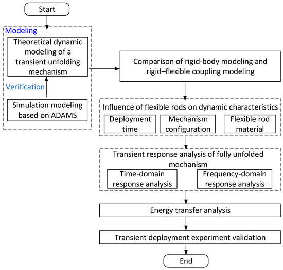
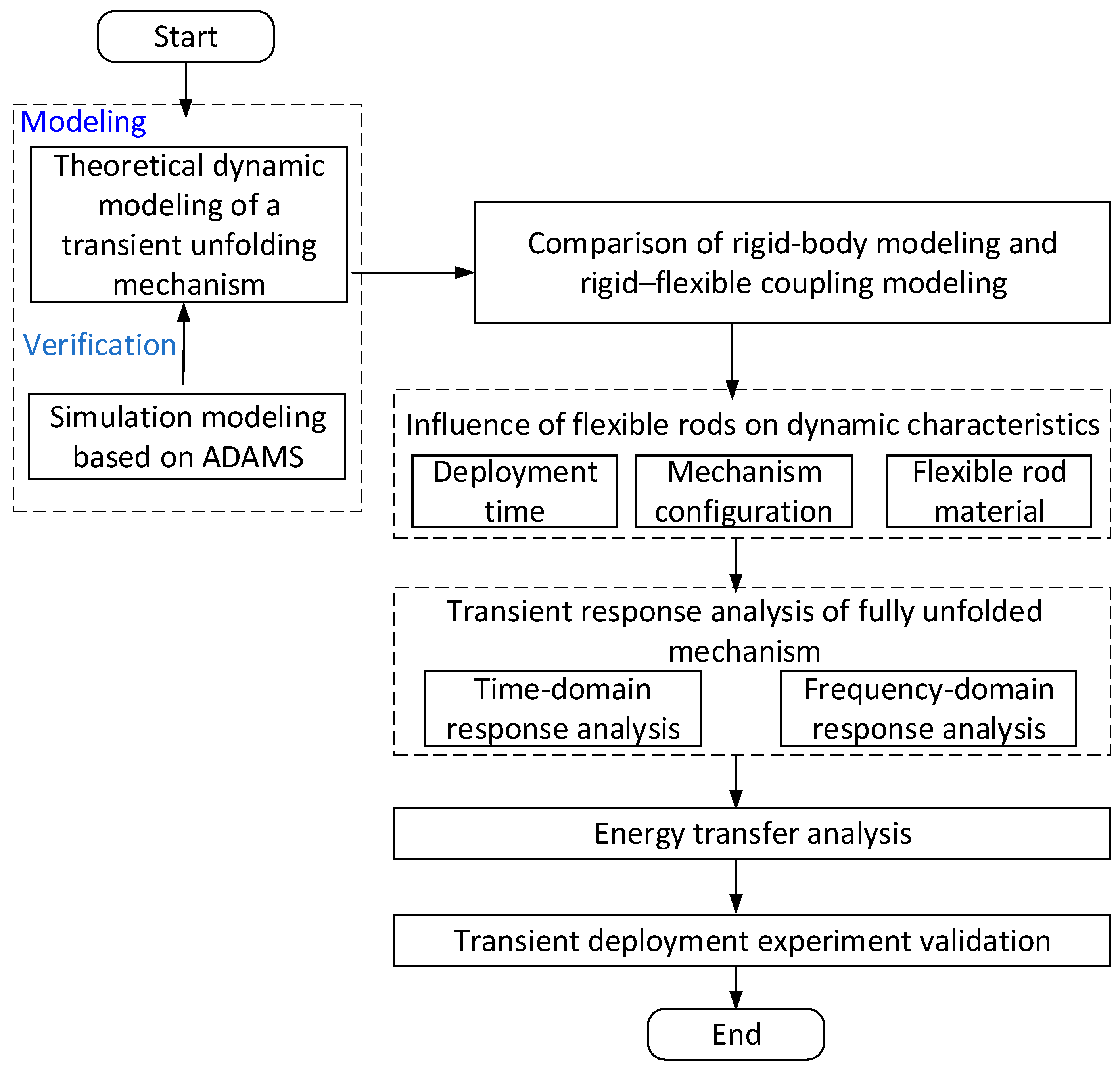
The organization of the paper is illustrated in u Figure 1. Section 2 develops a rigid–flexible coupled dynamic theoretical model for the deployment process of the transient unfolding mechanism based on the absolute nodal coordinate formulation ANCF. Section 3 validates the theoretical model against three-dimensional numerical simulations and, using the theoretical model, compares the dynamic responses of the rigid–flexible coupled model and the rigid-body model, analyzing the effects of deployment time, mechanism parameters and rod material properties on flexible rod deformation. Section 4 examines the dynamic response of the transient unfolding mechanism under four representative impact input signals. Section 5 investigates the energy evolution of the main system components during transient deployment to elucidate the mechanism of energy transfer. Section 6 presents experimental deployment tests that validate the proposed theoretical model. Finally, the main conclusions are drawn in Section 7.
Figure 1.
Technical roadmap for dynamic modeling and analysis of a transient unfolding mechanism.
2. Dynamic Modeling of Transient Unfolding Mechanism
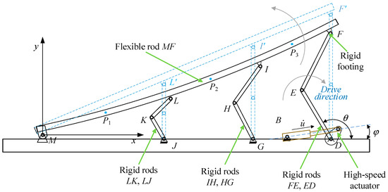
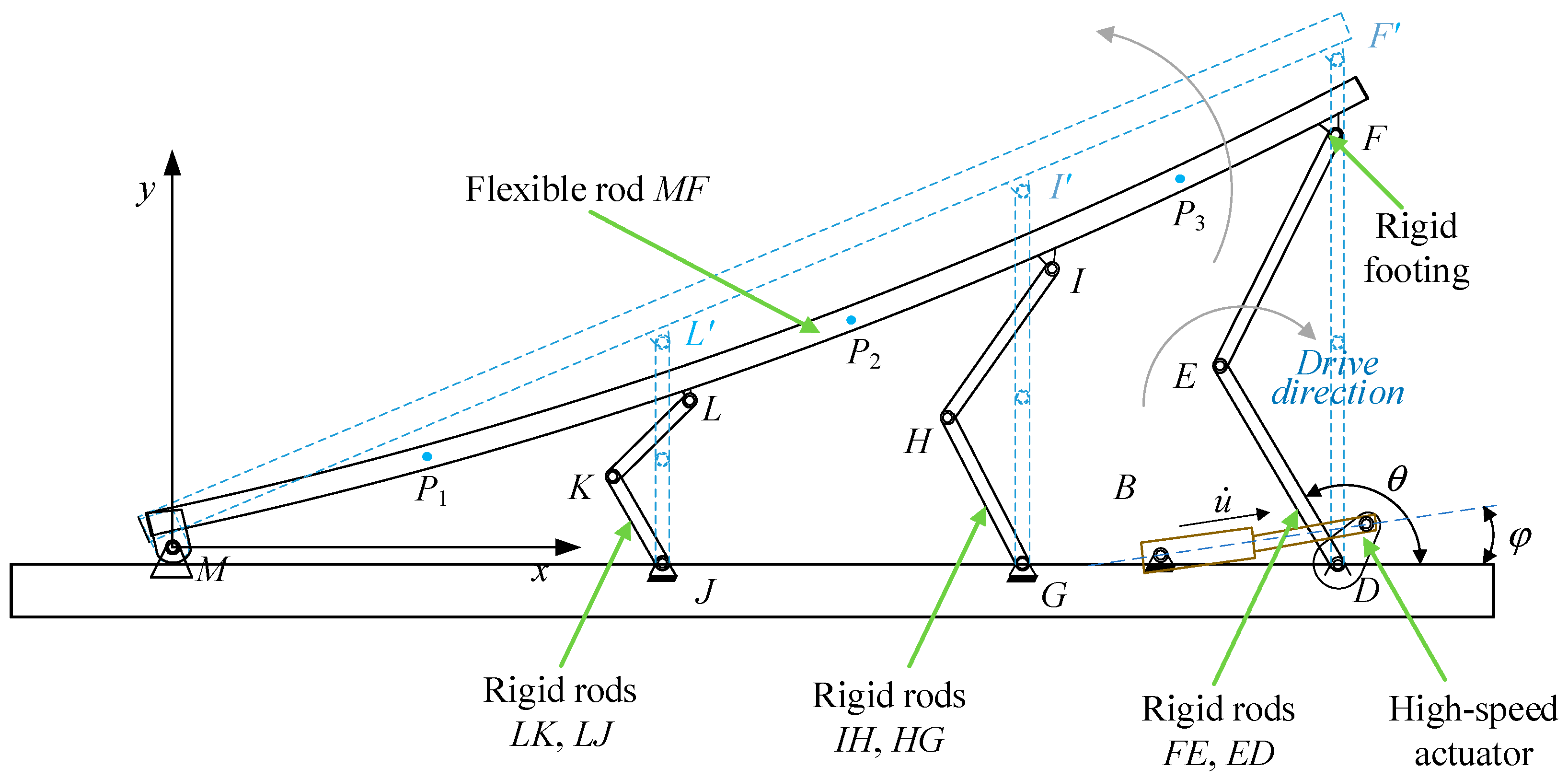
A transient unfolding mechanism is illustrated in Figure 2. Compared with previous morphing aircraft designs, the transient mechanism adopted in this work can achieve higher morphing speeds and withstand higher morphing accelerations [28,29]. The use of flexible rods enables a lighter overall structure and reduced inertial effects [30,31]. In addition, the structural configuration is simpler, which facilitates manufacturing and system integration [32]. However, during transient actuation, elastic deformation of the flexible rods may degrade the mechanism performance, thereby limiting its application scope. The mechanism consists of a flexible rod MF, rigid rods DE, GH, HI, JK, and KL, and a high-speed actuator. The rigid rods are connected to the flexible rod through rigid brackets. When driven by the high-speed actuator, the cam rotates and forces the flexible rod to bend through the rigid brackets, causing it to contact and collide with the moving rigid rods and thereby driving the mechanism to unfold rapidly. After reaching the fully deployed position, the mechanism locks immediately, and the flexible rod undergoes oscillation. Taking the rotation axis M of the flexible rod as the coordinate origin, the coordinate system is established as shown in Figure 2.
Figure 2.
Schematic of the transient unfolding mechanism.
The generalized coordinates of the rigid-link section can be expressed as follows:
The mass matrix of the rigid-link element is given by the following expression:
For the flexible link, its deformation is described using a two-node beam model. The displacement field of an arbitrary point P on the beam element in the inertial coordinate system is approximated by a polynomial function:
where a denotes the coefficients of the displacement field.
The absolute coordinates of the beam element nodes form a matrix composed of the values at its two endpoints. When the parameter s takes the values 0 and le, respectively, where le denotes the beam element length, the position vector r of any point on the flexible link can be expressed in terms of the absolute nodal coordinates q as:
where S denotes the shape functions of the beam element relative to the inertial basis, defined as:
where
The generalized mass matrix of the flexible rod can be expressed using the mass matrix of the beam element as follows [33]:
where denotes the density of the flexible rod, and V represents its volume.
When subjected to transient actuation, the flexible link undergoes elastic deformation. The deformation of the element includes an axial deformation vector and a tangential deformation vector . The strain energy expression for the beam element is:
From Equation (8), the stiffness matrix of the beam element can be obtained as:
Using the element shape functions from Equation (5), the generalized distributed gravity for a flexible rod can be obtained:
where is the mass of the flexible body element.
The Lankarani-Nikravesh contact model [34] is employed to characterize the rigid-flexible collisions during deployment. While the model simplifies stress wave effects and residual deformations, it is well-suited for capturing the macro-transient dynamic coupling and high-restitution impacts of the current mechanism.
To characterize the internal energy dissipation of the flexible rods, the Rayleigh damping model is adopted. The damping matrix C is defined as a linear combination of the mass matrix M and stiffness matrix K:
where a and β are the mass-proportional and stiffness-proportional damping coefficients, respectively.
By substituting and assembling the mass matrices, elastic forces, external forces, and constraint equations of each element in the system, the dynamic equations of the transient deployment mechanism can be obtained [35]:
where and represents the elastic forces and generalized external force matrix, respectively; represents the system constraint equations; and is the Lagrange multiplier vector. Equation (14) is solved using the generalized-α method.
3. Influence of Flexible Rods on the Motion Characteristics of Transient Systems
3.1. Comparison Between the Theoretical Model and the Simulation Model
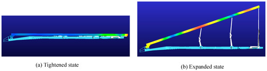
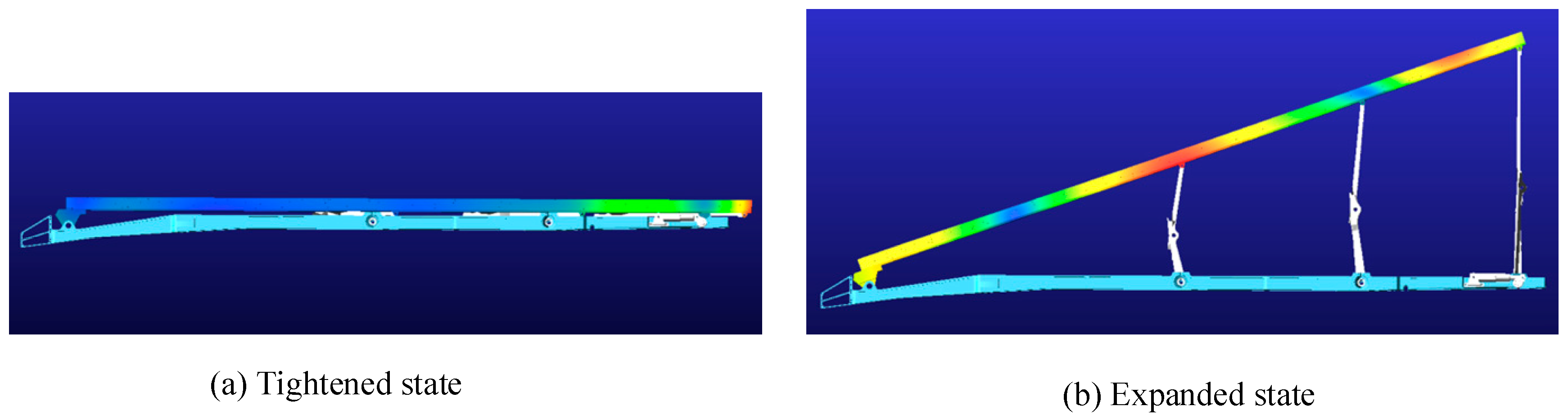
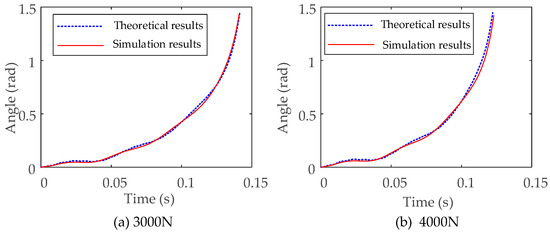
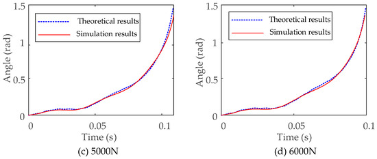
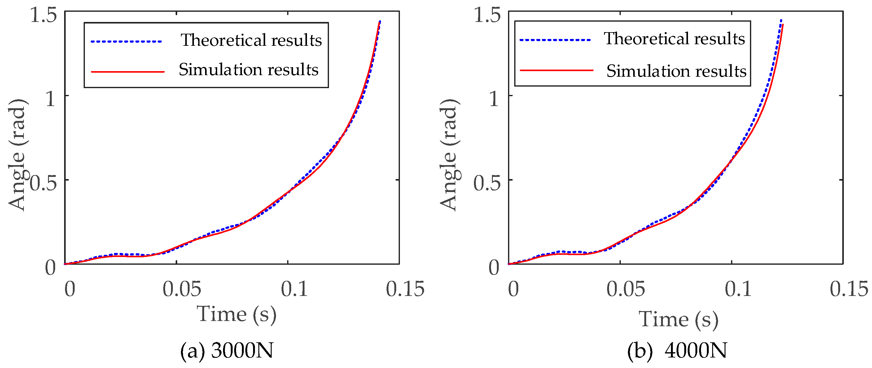
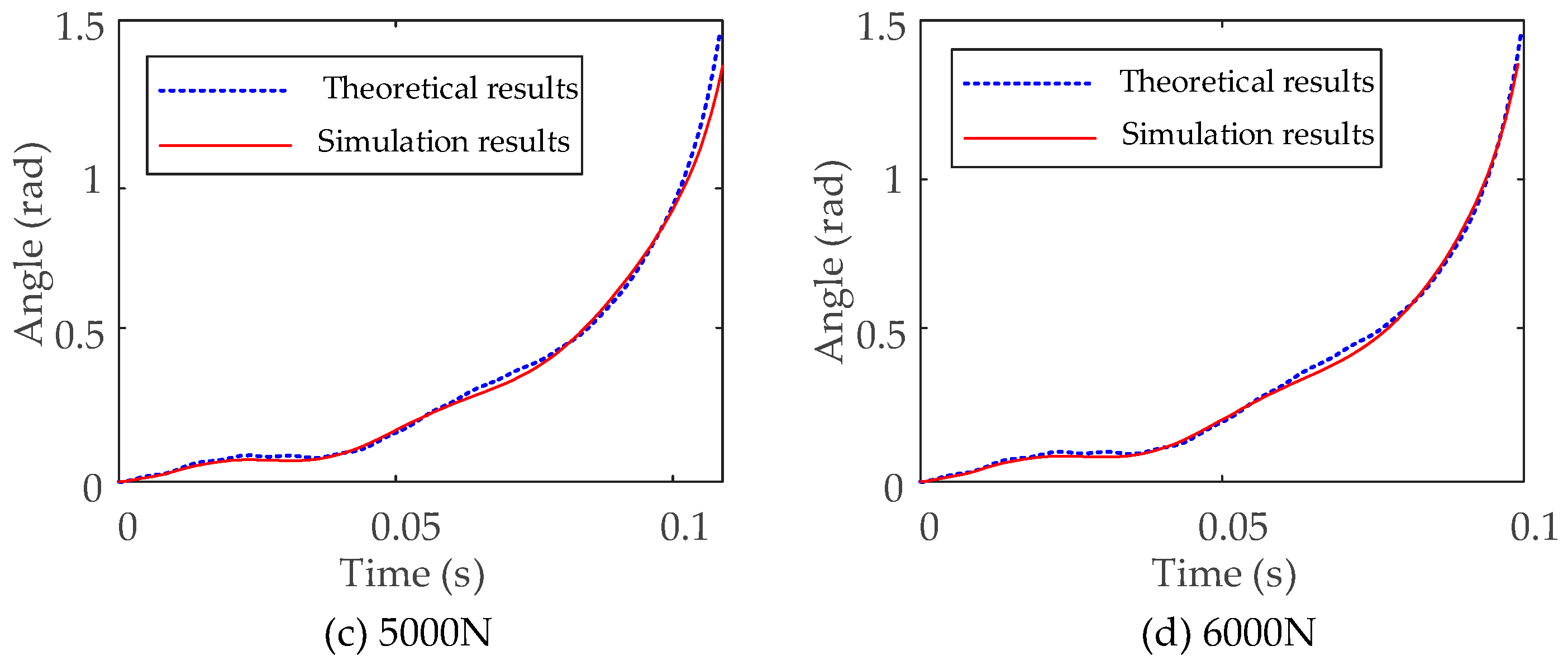
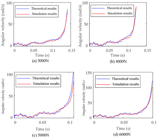
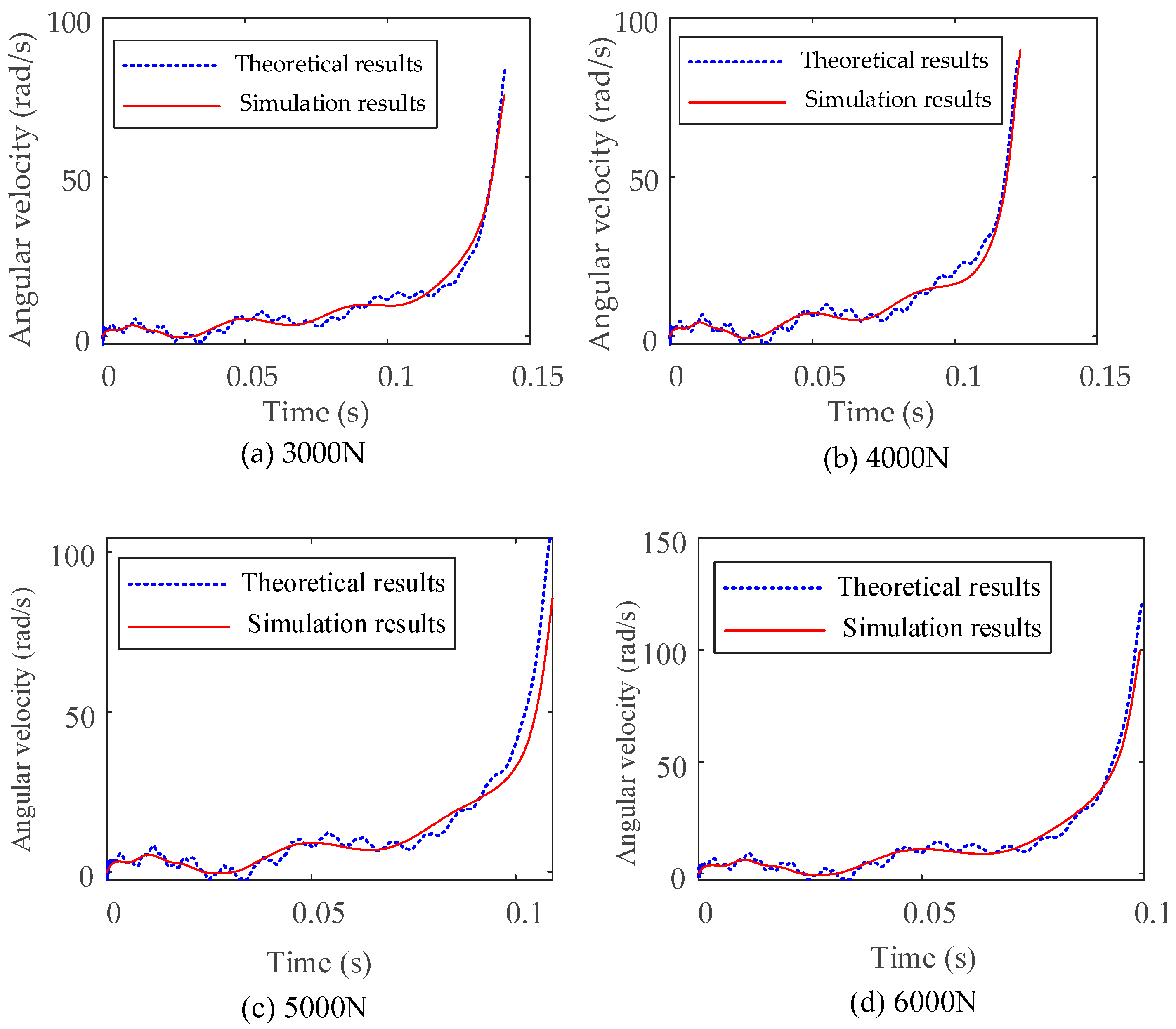
To verify the accuracy of the theoretical model established in Section 2, as shown in Figure 3, a rigid-flexible coupling dynamic model for the transient folding mechanism was developed through a joint simulation using ADAMS 2024.1 and ABAQUS 2024. The workflow involved importing the CREO assembly into ADAMS for defining constraints and contact parameters. ABAQUS was then utilized to generate flexible bodies by extracting modal data to replace rigid components. The final dynamic analysis was performed using the modal superposition method within the ADAMS environment. A comparative analysis was conducted between the results of the theoretical model and the simulation model. The parameters of the flexible rod are shown in Table 1, Figure 4 and Figure 5, respectively, present the comparison results of the angular displacement and angular velocity of rod DE in the transient unfolding mechanism between the rigid-flexible coupled dynamic theoretical model and the simulation model.
Figure 3.
Rigid-flexible coupling simulation model of transient unfolding mechanism.
Table 1.
Flexible rod related parameters.
Figure 4.
Comparison of rod DE angular displacement between theoretical and simulation models.
Figure 5.
Comparison of rod DE angular velocity between theoretical and simulation models.
In Figure 4, the flexible rod causes the motion curve of the mechanism to exhibit some fluctuations. Although the numerical results and the curve fluctuations are generally consistent, there are subtle differences in the frequency and amplitude of the fluctuations between the two, resulting in an error where the curves oscillate up and down. The theoretical model’s calculation results are generally higher. From Figure 5, the angular velocity results of rod DE in both the theoretical model and the simulation model show consistent overall trends. While the simulation results exhibit large fluctuations, the curve remains relatively smooth. In contrast, the theoretical results clearly exhibit high-frequency vibration components.
Furthermore, to quantitatively assess the alignment between the two methodologies, the discrepancy was measured using the Root Mean Square Error (RMSE), while the Normalized Root Mean Square Error (NRMSE) and the Coefficient of Determination (R2) were utilized to characterize the relative error and the goodness of fit, respectively.
The RMSE is adopted to measure the absolute deviation between the predicted and simulated values:
where and represent the simulated and theoretical values at the i sampling point, respectively, n denotes the total number of samples.
NRMSE is a dimensionless metric used to evaluate the forecasting accuracy of models by scaling the RMSE relative to the range of the data. The NRMSE is calculated as follows:
where and are the maximum and minimum values of the theoretical results within the observed range.
The R2 value measures the goodness of fit between the model and the data, where a value closer to 1 indicates a stronger correlation in trend. The R2 is calculated as follows:
where is the mean value of the theoretical data.
The calculated RMSE, NRMSE, and R2 values for the theoretical and simulation models are summarized in Table 2. The statistical metrics demonstrate a high degree of fidelity between the proposed theoretical model and the numerical simulations. Specifically, across the four analyzed operating conditions, the maximum NRMSE is 4.77%, while all R2 coefficients consistently exceed 0.97. The theoretical predictions are generally consistent with the simulation results, indicating that the rigid-flexible coupled model of the transient unfolding mechanism, established using the ANCF, is highly reliable.
Table 2.
The RMSE, NRMSE and the R2 values for the theoretical and simulation models.
3.2. Analysis of the Influence Factors of Flexible Rods on Transient Systems
- (1)
- Comparison between rigid body dynamics model and rigid-flexible coupling model
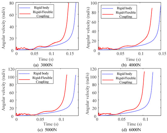
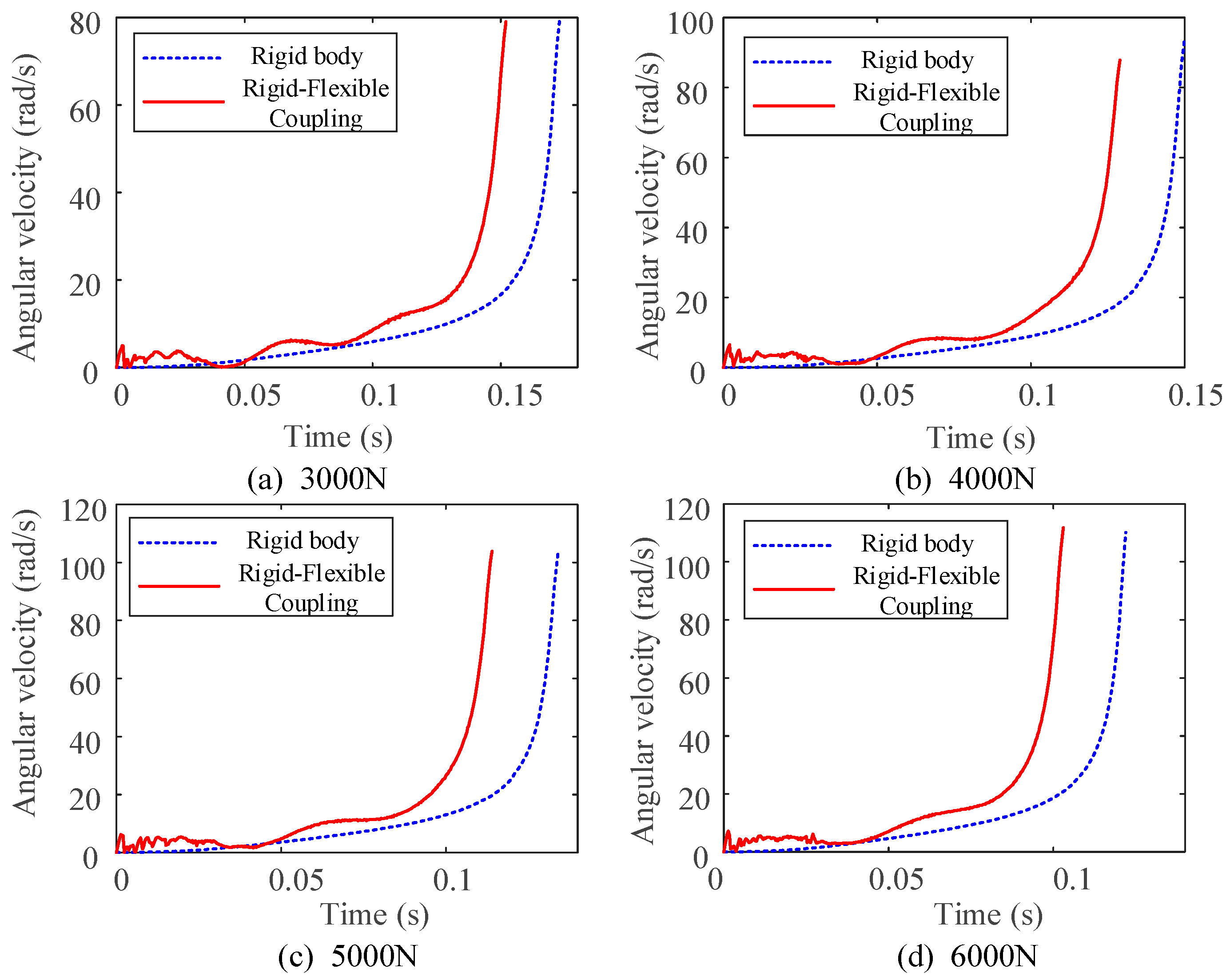
Four different driving input forces of 3000 N, 4000 N, 5000 N, and 6000 N were applied to both the rigid body dynamics model and the rigid-flexible coupled dynamics model. The angular velocity comparison curves of rod DE were plotted, as shown in Figure 6, to explore the motion differences in the mechanism under different driving forces.
Figure 6.
Comparison of the angular velocity of rod DE in the rigid body model and the rigid-flexible coupling dynamics model under different driving conditions.
In Figure 6, the motion trends of rod DE under both models are generally the same, and the final angular velocity at the target position is almost identical. Under the same driving force, the flexible design reduces deployment time by 15.57% compared with the rigid design However, the presence of the flexible body results in a shorter settling time for the mechanism. The angular velocity curve also differs from the smooth curve of the rigid body model, exhibiting fluctuations. The larger the driving force, the fewer the number of fluctuations.
- (2)
- Comparison of deformation under different expansion times
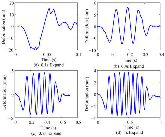
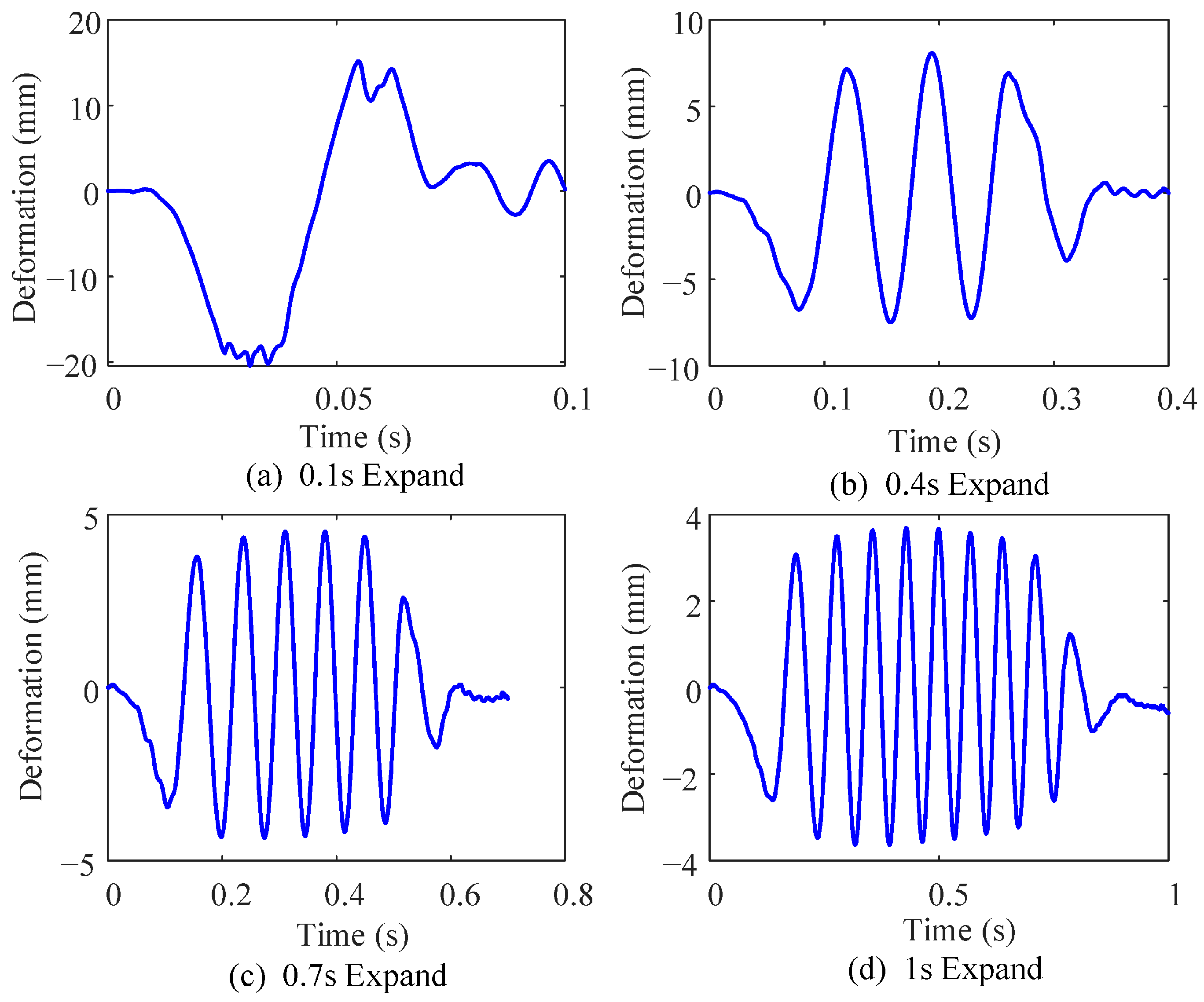
The deformation of a point on the flexible rod is used as an indicator to measure the degree of deformation of the flexible rod. Four different unfolding times of 0.1 s, 0.4 s, 0.7 s, and 1.0 s are set, and the deformation results of the flexible rod for each group are compared, as shown in Figure 7.
Figure 7.
Comparison of deformation at different unfolding times.
The deformation curve of the flexible rod changes over time, initially experiencing a downward peak followed by distinct periodic oscillations, and significantly attenuating in amplitude in the final phase. The shorter the unfolding time, the larger the amplitude of the flexible rod, and the greater the strain energy absorbed by the vibration. As the time scale increases, the flexible rod absorbs and releases strain energy by reducing the amplitude and increasing the duration of vibration. This reflects that the force acting on the flexible rod during transient motion is much greater than that during low-speed motion.
- (3)
- Effect of the intermediate link on the deformation of the flexible rod
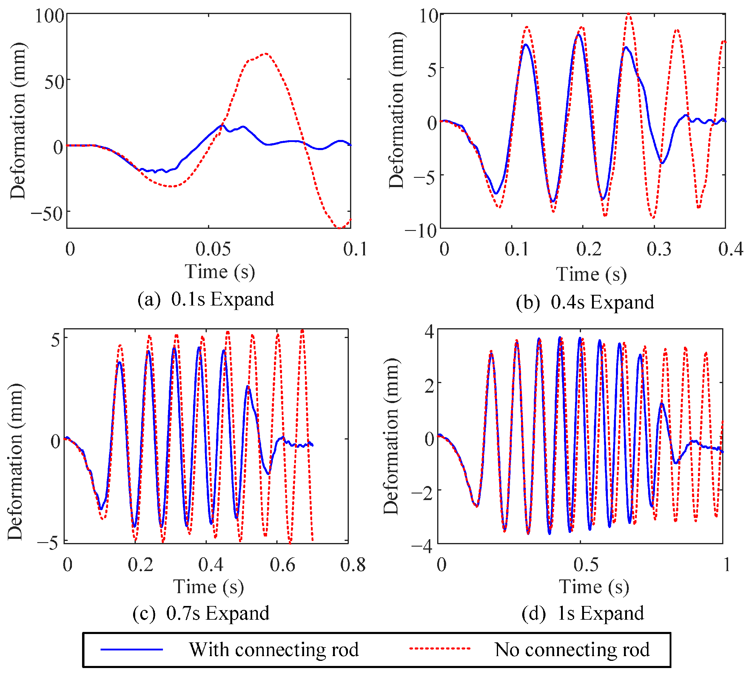
The flexible link MF of the transient unfolding mechanism is connected by three sets of rigid links. To study the effect of the intermediate links on the deformation of the flexible link, the two intermediate link sets, JKL and GHI, are removed, and time variables are set at 0.1 s, 0.4 s, 0.7 s, and 1.0 s. Figure 8 shows a comparison of the shape changes in the flexible link with and without the intermediate links. In the early stages of motion, both systems exhibit periodic oscillations at almost the same frequency. The amplitude of the system without the intermediate link is slightly larger than that of the system with the link. As the unfolding time increases, the amplitude difference between the two systems gradually decreases. In the later stages of motion, the system with the intermediate link undergoes irregular oscillations that quickly attenuate, while the system without the link shows little amplitude decay. This indicates that the presence of the intermediate link can effectively suppress the vibration deformation of the flexible rod, reducing its deformation, with a more pronounced suppression effect at shorter unfolding times.
Figure 8.
Comparison of deformation with and without intermediate flexible link.
- (4)
- Influence of flexible rod material on deformation of flexible rod
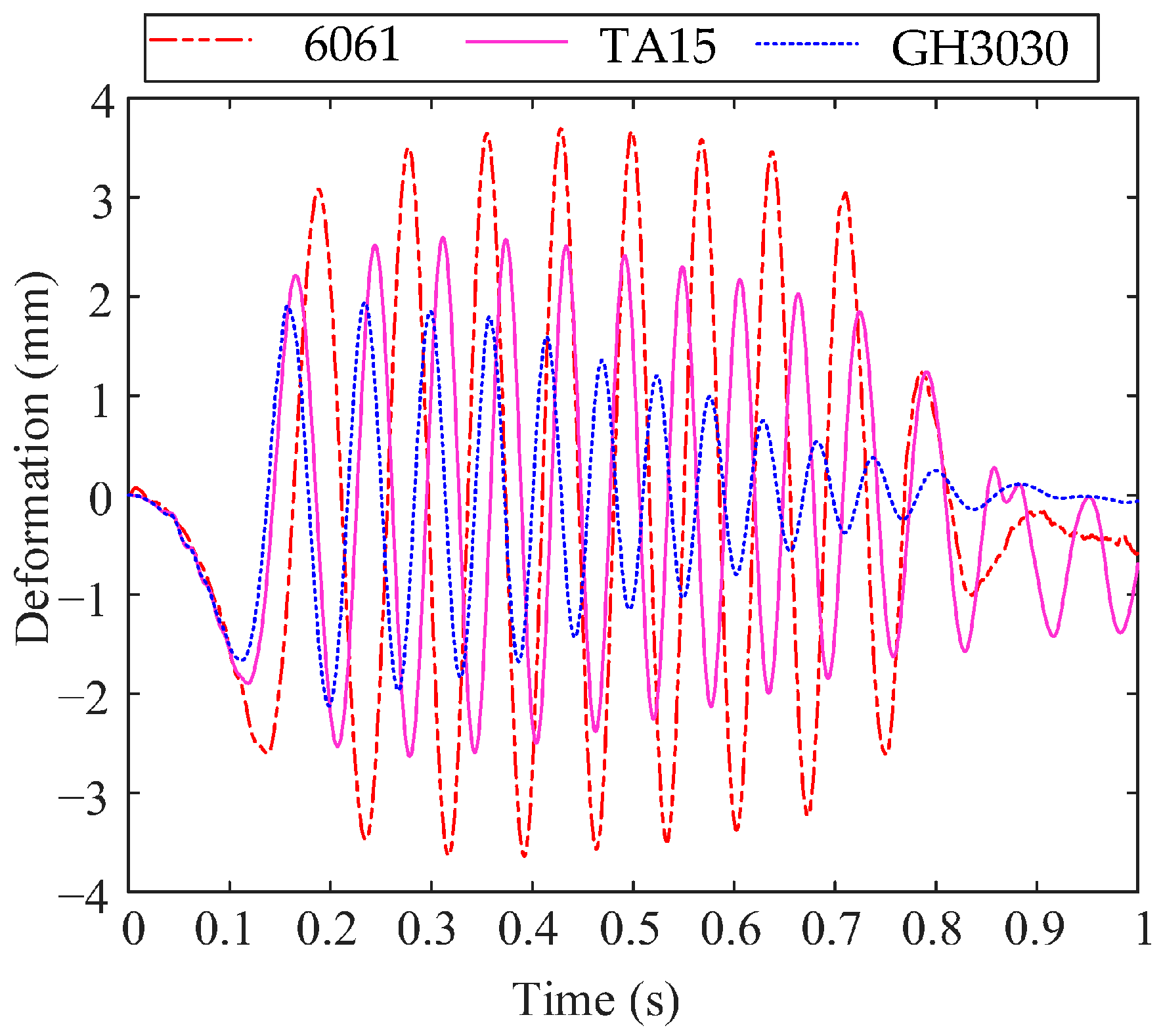
To study the effect of different flexible rod materials on its deformation, three metal materials—aluminum alloy 6061, titanium alloy TA15, and high-temperature alloy GH3030—were selected as the material parameters for analysis. The material parameters of these three materials are shown in Table 3. The deployment time was set to 1.0 s, and the calculation results are shown in Figure 9.
Table 3.
Flexible rod material parameters.
Figure 9.
Deformation changes in flexible rods made of three different materials.
As shown in Figure 9, the deformation of the flexible rods made of the three materials exhibits a periodic decaying oscillation. Throughout the process, the aluminum alloy rod shows the largest deformation, followed by the titanium alloy rod, while the high-temperature alloy exhibits the smallest deformation.
4. Transient Response Analysis
4.1. Classic Shock Signal
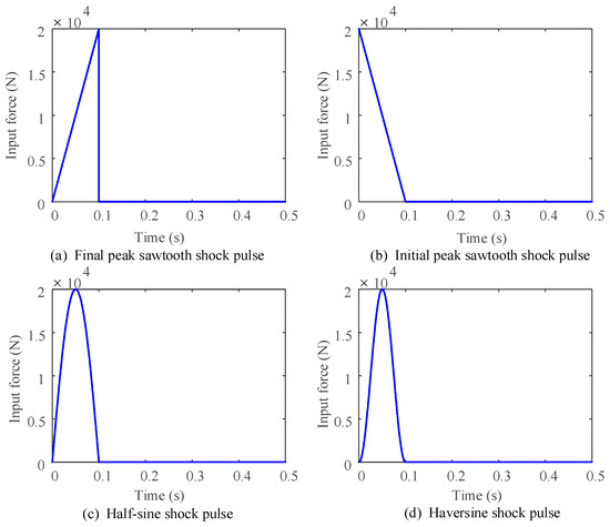
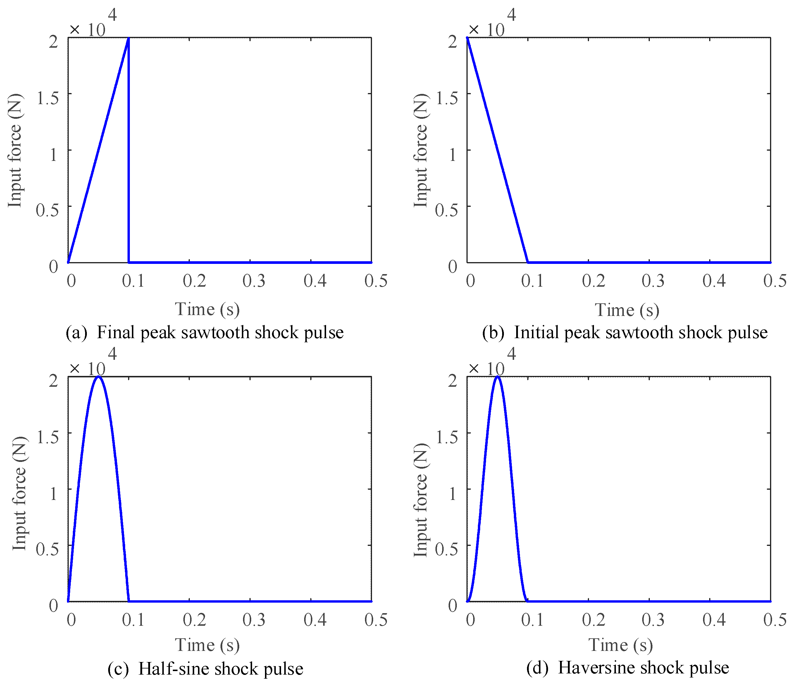
In the absence of actual measurement data, four classic impact signals were used as input conditions to study the transient response characteristics of the transient unfolding mechanism, especially the flexible rod under transient drive. This paper uses four classic impact signals as inputs: final peak sawtooth shock pulse, initial peak sawtooth shock pulse, Half-sine shock pulse, and half-ramp shock pulse as shown in Figure 10.
Figure 10.
Four classic shock signals.
4.2. Time-Domain Response Analysis
- (1)
- Angular displacement and angular velocity response
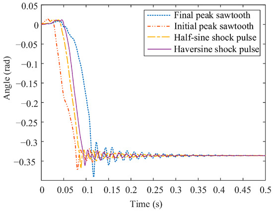
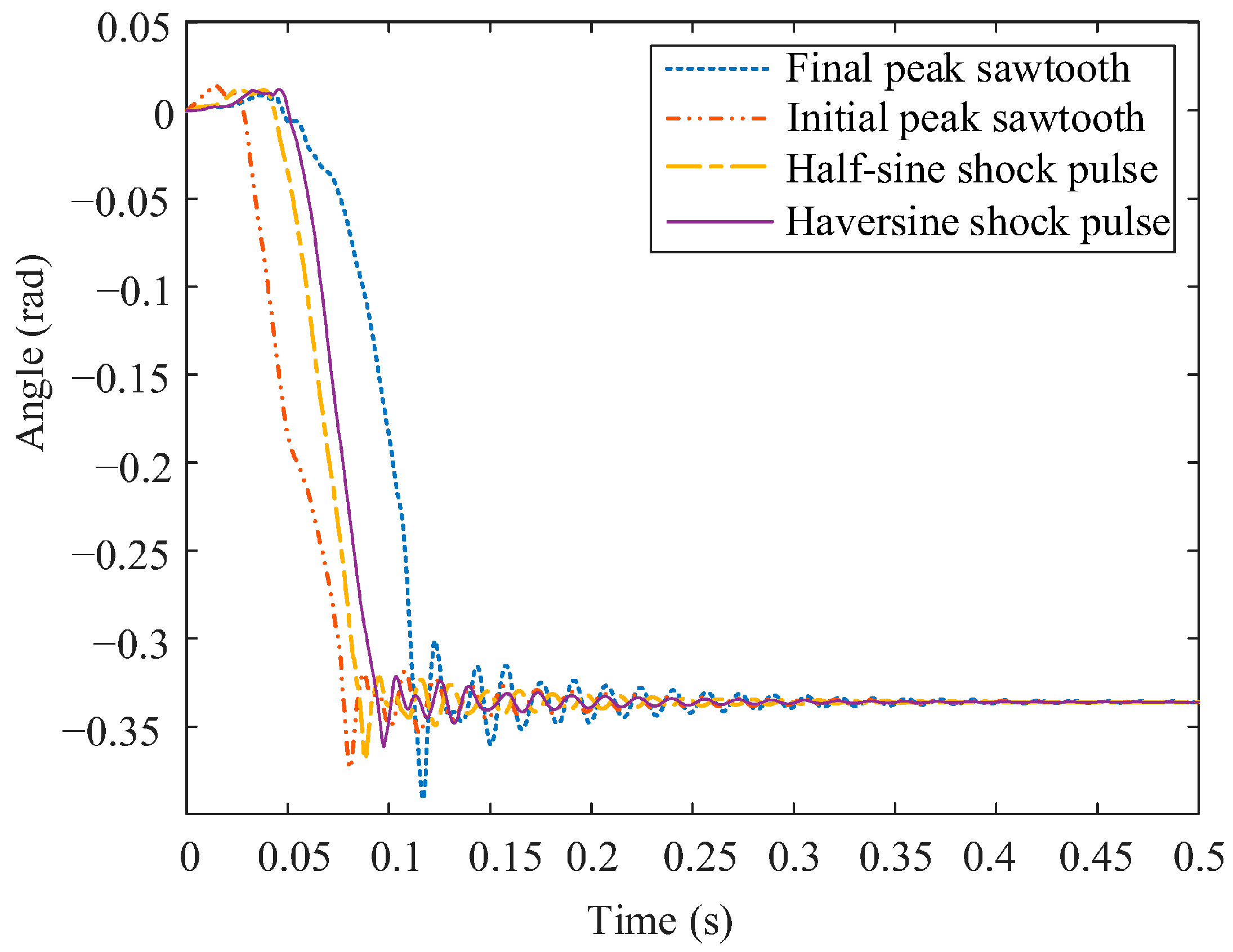
Using four classic shock pulses as input, the time-varying angular displacement of the flexible member is analyzed under four different conditions to obtain its displacement response. As shown in Figure 11, the transient driving force at the initial stage of the shock has a significant impact on the response time of the deployment motion and the reverse angular displacement response. The greater the initial transient driving force, the quicker the response of the deployment motion, and the higher the peak value of the reverse angular displacement response. This further indicates that the deformation caused by the transient shock on the flexible member is greater at this moment. The flexible member deployment speed response under the four types of shock pulses is shown in Table 4. From the angular displacement and angular velocity responses of the flexible member under different shock inputs, it can be observed that the angular velocity response of the flexible member can be divided into two stages: deployment motion and vibration after reaching the final position.
Figure 11.
Deployment displacement response of the flexible member under different shock inputs.
Table 4.
Peak response time and reaching stability time of flexible rod deployment speed under different impacts.
Based on the analysis of displacement and velocity responses, triangular shock pulses have a greater impact on the system’s response when the peak occurs either at the start or the end. If the peak input force occurs at the start, the flexible component exhibits the largest reverse displacement, i.e., the maximum initial deformation. If the peak input force occurs at the end, the peak of the system’s displacement velocity response is the largest. Compared to triangular shock pulses, sine wave pulses have a smaller transient impact on the system, and among them, the half-haversine shock pulse, with its smaller force rate of change at both the start and the end, causes the least transient impact. Under the half-haversine shock pulse, the system’s velocity response peak is the smallest, and the time required for the peak to decay to a stable value is the shortest.
- (2)
- Flexible rod deformation response
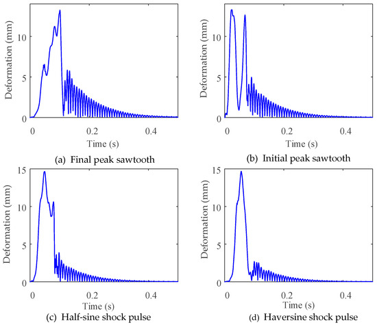
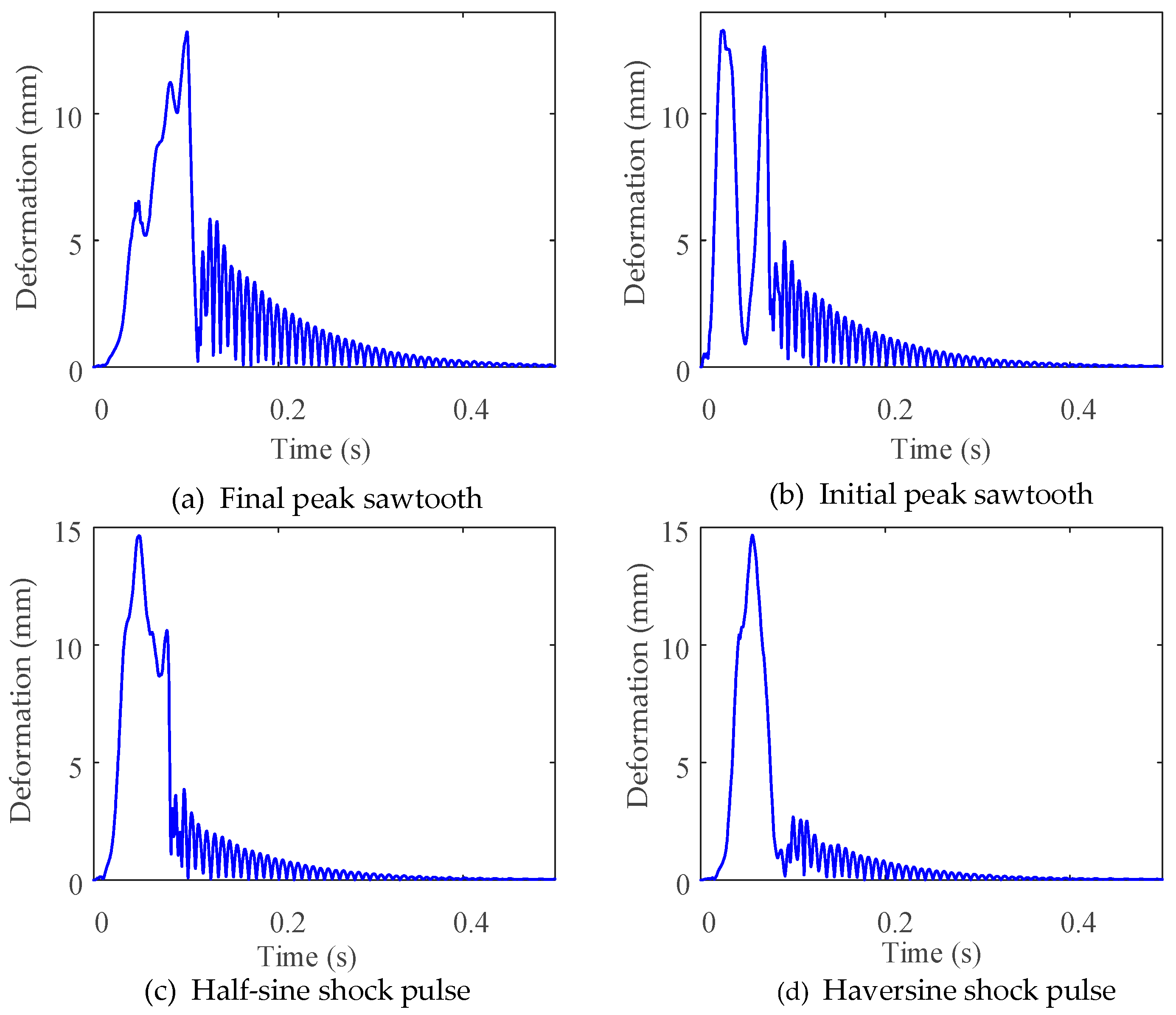
Three test points are selected between adjacent rotational pairs of the flexible rod to represent the deformation status of each section of the flexible rod. The distribution of the test points is shown in Figure 2. Taking point P2 as the research object, four classic impact signals are used as inputs, and the total deformation of point P2 is measured, with the curves plotted as a function of time, as shown in Figure 12.
Figure 12.
Deformation response of flexible rod at P2 point under different impact inputs.
Under the final peak sawtooth shock pulse, the deformation of the mechanism during the unfolding stage is relatively small, and the impact at the final position has the smallest effect on the deformation of the flexible rod compared to the other three shock types. After reaching the final position, the flexible rod still exhibits considerable vibrational deformation. However, under the Haversine shock pulse, the deformation during the unfolding stage is slightly larger, and the impact at the final position has the greatest effect on the deformation of the flexible rod. After reaching the final position, the vibrational deformation of the flexible rod is significantly smaller than that under the final peak sawtooth shock pulse. Integrating the observations from Figure 10, the form of the deformation response during the unfolding process of the flexible rod is largely determined by the type of shock input.
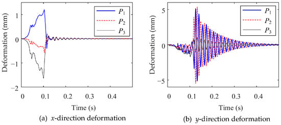
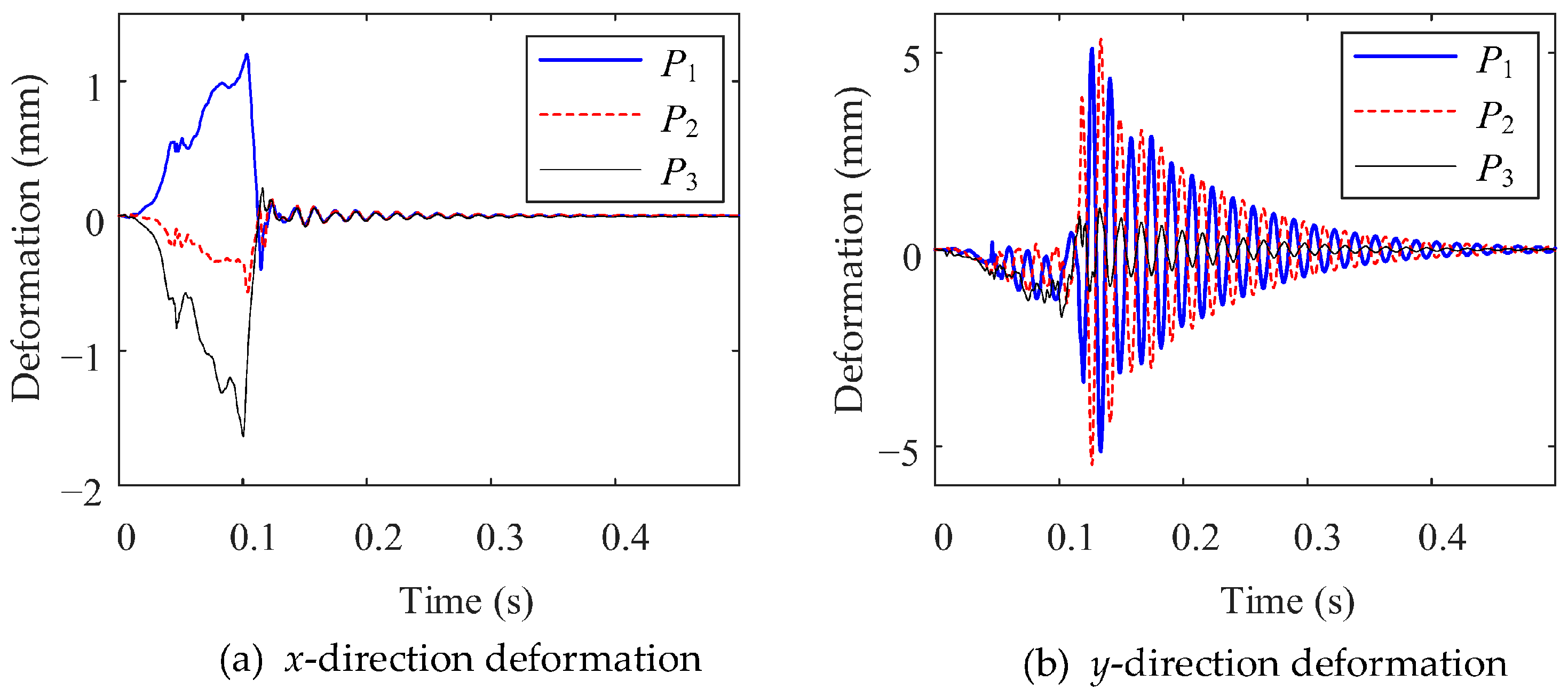
Using the final peak sawtooth shock pulse as the driving input, three test points P1, P2, and P3 are selected as the research objects to measure the directional deformation responses and overall deformation response in different directions under transient shock conditions, as shown in Figure 13, to study the overall deformation response of the flexible rod under transient shock. Under transient shock, among the three measurement points, P1 consistently exhibits the largest deformation amplitude. Considering that the flexible-rod segment at P1 is the longest, this indicates that the greater the distance between the two rotational pairs of the flexible rod, the more pronounced the deformation becomes. This indirectly demonstrates that the presence of the intermediate link effectively suppresses the deformation of the flexible rod.
Figure 13.
Deformation response of a flexible rod to a final-peak sawtooth shock input.
4.3. Frequency Domain Response Analysis
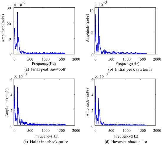
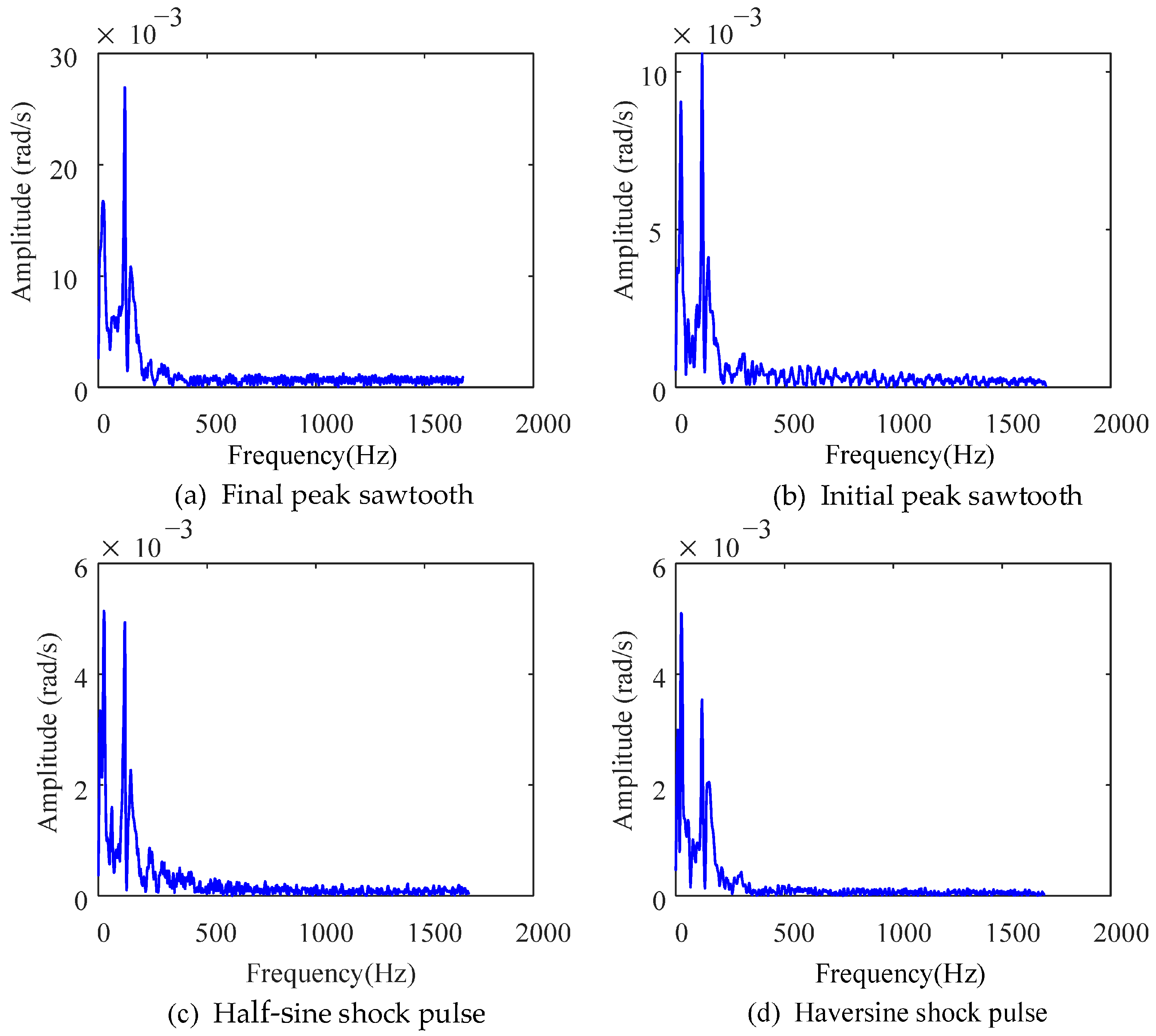
Fourier transform (FFT) was performed on the flexible rod displacement velocity response under four types of impact in the time-domain analysis, obtaining the flexible rod’s displacement velocity response in the frequency domain, as shown in Figure 14. The displacement speed response of the flexible rod has higher amplitude in the low-frequency range, and all four operating conditions exhibit three peak values in the velocity response. The three response peak values and their corresponding frequency data are summarized in Table 5.
Figure 14.
The displacement speed response of the flexible link in the frequency domain.
Table 5.
Speed response peak values and their corresponding frequencies.
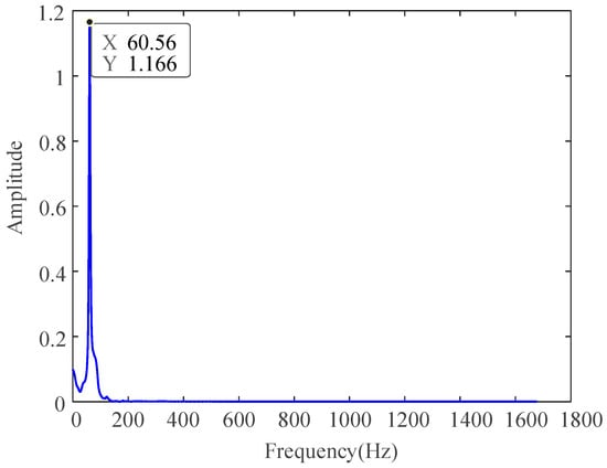
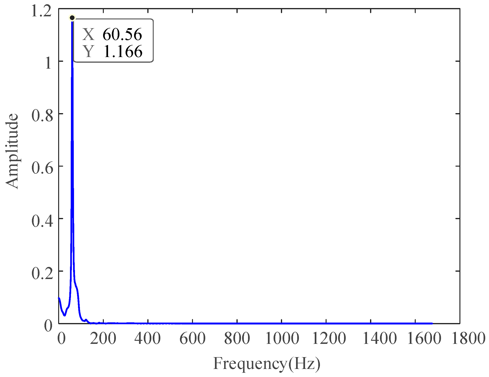
Under different shock inputs, the three peak values of the flexible rod’s displacement velocity frequency-domain response generally occur near frequencies of 23 Hz, 121 Hz, and 150 Hz. Moreover, it can be clearly observed from the Table 5. that, in the frequency domain, the three response peak values under the final peak sawtooth shock are significantly larger than those under the other three conditions, while the response peaks under the half-sine shock are the smallest. In-depth research into the frequency-domain characteristics of the flexible rod’s vibration during the settling phase reveals that the time-domain deformation response in the Y-direction at P1 under the final peak sawtooth shock is processed using FFT to obtain the corresponding frequency-domain response, as shown in Figure 15. From Figure 15, it can be seen that in the frequency-domain analysis, the deformation response of the flexible rod at point P1 in the Y-direction exhibits only one peak, with the corresponding frequency of 60.56 Hz. Since the motion in the settling vibration phase is essentially free vibration, it is independent of the input force and only related to the inherent characteristics of the flexible rod. To further analyze the deformation response characteristics of the flexible rod, modal analysis is performed using finite element software to extract the first six natural frequencies, which are recorded in Table 6. Based on the modal analysis of the flexible rod, it can be observed that the deformation response frequency during the settling vibration phase is close to the fifth natural frequency of the flexible rod, meaning that the energy during the settling vibration phase is concentrated at the fifth natural frequency.
Figure 15.
Final peak sawtooth shock P1 point Y-direction frequency-domain deformation response.
Table 6.
The first six natural frequencies of the flexible rod.
5. Energy Transfer Analysis
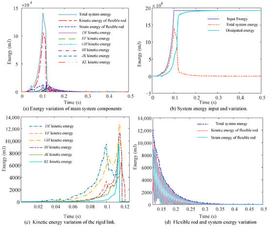
The peak value of the input is 20,000 N with a duration of 0.1 s for the final peak sawtooth wave shock. The analysis focuses on studying the energy transfer law of the transient unfolding mechanism with a flexible body during its unfolding motion under transient shock. During the motion, the total system energy of the transient unfolding mechanism primarily includes the kinetic energy and strain energy of the flexible rod and the kinetic energy of the six rigid linkages. The kinetic energy of other components is much smaller than the above-mentioned energies and can thus be neglected. The system energy transfer is shown in Figure 16.
Figure 16.
Energy transfer of the transient unfolding mechanism system.
Energy variation in the main moving components is shown in Figure 16a. It can be observed that throughout the entire motion process, the system energy is primarily concentrated in the kinetic and strain energy of the flexible rod, with the kinetic energy of the rigid bodies accounting for a smaller proportion. During the flexible rod’s unfolding phase, the system energy includes the strain energy and kinetic energy of the flexible rod, as well as the kinetic energy of the rigid linkages. Among these, the kinetic energy of the flexible rod is much greater than the energy of the other parts.
Further comparison is made between the input energy, total system energy, and the dissipated energy represented by their difference. As shown in Figure 16b, the total system energy variation can be divided into four stages. The first stage is the rapid unfolding phase, where the total system energy change is closely related to the input energy, and the rate of increase continues to rise. The second stage is the transition phase between the end of the impact input and the final collision, where, due to the lack of external force input and the damping effects in the system, the total system energy rapidly decreases. The third stage is the final collision phase, where all components collide and stop moving. In a very short period, the rigid body kinetic energy becomes zero, and the kinetic energy of the flexible rod significantly decreases, causing the total system energy to drop sharply. The fourth stage is the post-final collision flexible rod vibration phase, where the system energy dissipates slowly at a small rate.
The kinetic energy variation curves of the three rigid linkages are shown in Figure 16c. Under transient impact, due to the elastic deformation of the flexible rod caused by the impact, the motion of each linkage no longer remains synchronized. The motion transmission of the mechanism exhibits hysteresis, with the linkages farther from the drive source reaching their final positions more quickly, while the linkages closer to the drive source experience more intense motion fluctuations.
The variation curves of the kinetic energy, strain energy, and total system energy of the flexible rod during the final vibration phase are shown in Figure 16d. In this phase, the total system energy continuously decays to zero. The variation curves of the flexible rod’s kinetic energy and strain energy oscillate at the same frequency, but there exists a phase difference in size between the two. This indicates that the kinetic energy and strain energy of the flexible rod are constantly transforming into each other at a specific frequency, with the external manifestation being the damped oscillations of the flexible rod after reaching the final position.
To further determine the frequency of the transformation between the flexible rod’s kinetic energy and strain energy, a Fourier transform was applied to the strain energy variation curve in Figure 16d. It was found that the frequency domain response of the strain energy has a peak at a frequency of 122.2 Hz, which is approximately twice the frequency of the peak deformation response at point P1 in the y-direction of the flexible rod. This suggests that the kinetic energy and strain energy of the flexible rod transform into each other at this frequency, while the vibration frequency during the final position phase of the flexible rod is 60.56 Hz.
6. Transient Deployment Experiment Validation
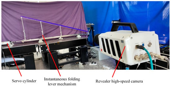
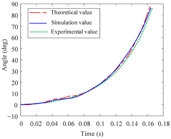
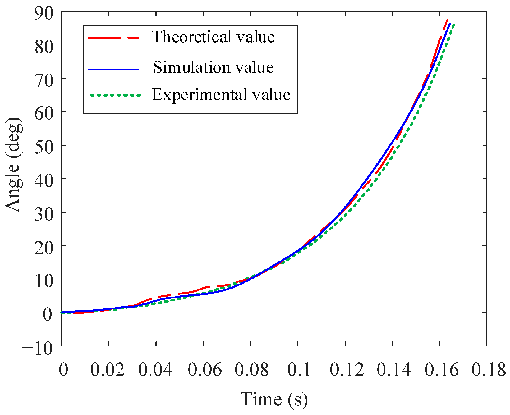
To verify the accuracy of the theoretical model established in this paper, a transient unfolding mechanism prototype was designed and fabricated, and transient deployment tests were conducted. As shown in Figure 17, the flexible rods were fabricated using GH3030 superalloy to accommodate high-temperature flight conditions. To achieve rapid deployment, a Panasonic MSMF82L1U2M servo electric cylinder with a rated power of 750 W and a rated torque of 2.39 N·m was selected to provide the driving force. A Zhongke Shijie X113 high-speed camera with a resolution of 1280 × 1024 and a maximum sampling rate of 500,000 fps was used for motion data acquisition, which was combined with input force data extracted from an S-type load cell to form a complete set of experimental input-output data. The deployment time of the mechanism is set to 0.162 s. A comparison of the angular displacement during the DE deployment phase obtained from the theoretical model, simulation, and experiment is shown in Figure 18. The calculated RMSE, NRMSE, and R2 values for the comparisons among the theoretical, simulation, and experimental results are summarized in Table 7.
Figure 17.
Deployment experiment of transient mechanism.
Figure 18.
Comparison of angular displacement in the DE deployment phase: theory, simulation, and experiment.
Table 7.
The RMSE, NRMSE and R2 values for the theory, simulation, and experiment results.
As illustrated in Figure 18 and Table 7, the results from both the theoretical and simulation models are in good agreement with the experimental curves. This consistency is further quantified by statistical indicators: the R2 values reach 0.94 and 0.97, respectively, indicating a high degree of fitting. The low RMSE and NRMSE values demonstrate minimal deviation from the experimental data, thereby preliminarily corroborating the validity of the previously established theoretical and simulation models. Notably, the theoretical and simulation results are more closely aligned with fewer oscillations, whereas the experimental curve exhibits a slightly lower magnitude and a smoother overall profile.
7. Conclusions
This paper investigates a transient unfolding mechanism incorporating a flexible rod. A rigid–flexible dynamic model of the mechanism was developed using the absolute nodal coordinate formulation (ANCF), and the model agrees well with simulation and experimental results. Based on this model, the influence of flexible-rod deformation on mechanism performance under transient driving conditions was analyzed, and the following conclusions were obtained:
- (1)
- Designs using flexible rods achieve faster deployment than all-rigid designs. Under the same driving force, the flexible design reduces deployment time by 15.57% compared with the rigid design; however, the deployment process exhibits oscillations, and increasing the driving force reduces the number of oscillation cycles.
- (2)
- The study quantifies how structural parameters affect reliability. Adding intermediate links effectively suppresses vibration-induced deformation of the flexible rod; without intermediate links, the vibration amplitude increases significantly. In terms of material performance, the high-temperature alloy GH3030 has superior deformation resistance compared with titanium alloy TA15 and aluminum alloy 6061, making GH3030 an ideal choice to improve reliability under high loads.
- (3)
- A comparison of four impact pulse shapes shows that the haversine pulse produces the smallest transient shock to the mechanism. For the same peak input, it yields the lowest peak velocity response and decays to a steady value fastest—only 0.1847 s, approximately 31% faster than the sawtooth pulse. This finding directly informs optimization of drive-source waveforms to extend mechanism service life.
The present work characterizes transient unfolding dynamics through a blend of theoretical, simulated, and experimental approaches, offering valuable insights for aerospace and robotic systems. However, current modeling omits flexible skin impacts and simplifies actuation forces; these elements are slated for inclusion in future high-fidelity iterations to improve performance prediction.
Author Contributions
Conceptualization, Y.B.; methodology, Y.B. and Y.J.; software, Y.B. and B.Y.; validation, Y.B.; formal analysis, Y.B.; investigation, Y.B.; resources, Y.B.; data curation, Y.B.; writing—original draft preparation, Y.B. and B.Y.; writing—review and editing, H.X. and R.Z.; visualization, Y.B.; supervision, R.L. and H.G.; project administration, H.X. and R.L.; funding acquisition, H.X., H.G., G.Y., R.Z. and R.L. All authors have read and agreed to the published version of the manuscript.
Funding
This research has received grants from the National Natural Science Foundation of China (NSFC) through grants Nos. 52192633, T2388101, 52405013, 12502054 and U2341237, the China Postdoctoral Science Foundation (Nos. 2023T160168 and 2024M764171), and the National Key Laboratory of Aerospace Mechanism (Grant No. 2025ASM-ZY10).
Institutional Review Board Statement
Not applicable.
Informed Consent Statement
Not applicable.
Data Availability Statement
The original contributions presented in the study are included in the article. Further inquiries can be directed to the corresponding author.
Conflicts of Interest
The authors declared no potential conflicts of interest with respect to the research, authorship, and publication of this article.
Abbreviations
The following abbreviations are used in this manuscript:
| ANCF | Absolute Nodal Coordinate Formulation |
References
- Jia, T.S.; Liu, C.R.; Shen, Z.G.; Wu, Z.S. Mechanism and effect factor of toughening of high-speed train wheels. Appl. Sci. 2023, 13, 8300. [Google Scholar] [CrossRef] [Scilit]
- Chen, Y.; Wu, X.Z.; Wang, H.C.; Yu, C.T.; Han, Z.H.; Wu, K. Prediction of nonlinear vibration characteristics for high-speed and ultra-precision mechanism with clearance joints. J. Sound Vib. 2023, 573, 118201. [Google Scholar] [CrossRef] [Scilit]
- Harris, M.; Jones, A.; Alexander, E. Miniature turbojet development at Hamilton sundstrand: The TJ-50, TJ-120 and TJ-30 turbojets. In Proceedings of the 2nd AIAA Unmanned Unlimited Conf. and Workshop & Exhibit, San Diego, CA, USA, 15–18 September 2003. [Google Scholar] [CrossRef] [Scilit]
- Interbartolo, M. Apollo Spacecraft and Saturn V Launch Vehicle Pyrotechnics/Explosive Devices; JSC-17237-4; National Aeronautics and Space Administration: Washington, DC, USA, 2009. [Google Scholar]
- Zhai, G.Q.; Tao, J.T.; Xiao, H.; Guo, H.W.; Yang, G.; Zhao, R.C.; Yao, C.; Liu, R.Q. Design of multi-wing deployment mechanism based on multiple performance indicators and topology: Theoretical and experimental Study. Appl. Sci. 2024, 14, 11672. [Google Scholar] [CrossRef] [Scilit]
- Xiao, H.; Li, S.L.; Guo, H.W.; Liu, H.L.; Yang, G.; Li, C.F.; Tao, J.G. Experimental study on dynamic force–thermal loading for multi-stage telescopic wings based on the dynamic multi-point equivalent method. Appl. Sci. 2025, 15, 2699. [Google Scholar] [CrossRef] [Scilit]
- Bai, Y.; Yang, G.; Guo, H.W.; Xiao, H.; Liu, R.Q.; Deng, Z.Q. An unsteady aerodynamic force calculation method for shear variable-sweep wing considering sweep angle and airfoil changes. Aerosp. Sci. Technol. 2024, 157, 109711. [Google Scholar] [CrossRef] [Scilit]
- Fang, Z.; Li, Z.; Jia, Z.Y.; Li, J.X.; Yu, J.Q. Dynamic modeling and observer-based fixed-time backstepping control for a hypersonic morphing waverider. Appl. Sci. 2024, 14, 5924. [Google Scholar] [CrossRef] [Scilit]
- Song, M.; Nam, T.; Lee, J. Self-Excited Torsional Vibration in the Flexible Coupling of a Marine Propulsion Shafting System Employing Cardan Shafts. J. Mar. Sci. Eng. 2020, 8, 348. [Google Scholar] [CrossRef] [Scilit]
- Gong, L.; Luo, W.J.; Chen, J.W.; Hua, Z.G. Rotor unbalanced vibration control of active magnetic bearing high-speed motor via adaptive fuzzy controller based on switching notch filter. Appl. Sci. 2025, 15, 3681. [Google Scholar] [CrossRef] [Scilit]
- Shabana, A.A. Definition of the slopes and the finite element absolute nodal coordinate formulation. Multibody Syst. Dyn. 1997, 1, 339–348. [Google Scholar] [CrossRef] [Scilit]
- García-Vallejo, D.; Escalona, J.L.; Mayo, J.; Domínguez, J. Describing Rigid-Flexible Multibody Systems Using Absolute Coordinates. Nonlinear Dyn. 2003, 34, 75–94. [Google Scholar] [CrossRef] [Scilit]
- García-Vallejo, D.; Mayo, J.; Escalona, J.L.; Domínguez, J. Three-dimensional formulation of rigid-flexible multibody systems with flexible beam elements. Multibody Syst. Dyn. 2008, 20, 1–28. [Google Scholar] [CrossRef] [Scilit]
- Liu, C.; Tian, Q.; Hu, H.; García-Vallejo, D. Simple formulations of imposing moments and evaluating joint reaction forces for rigid-flexible multibody systems. Nonliner Dyn. 2012, 69, 127–147. [Google Scholar] [CrossRef] [Scilit]
- Wang, Z.; Tian, Q.; Hu, H.Y. Dynamics of spatial rigid–flexible multibody systems with uncertain interval parameters. Nonliner Dyn. 2016, 84, 527–548. [Google Scholar] [CrossRef] [Scilit]
- Dombrowski, S.V. Analysis of large flexible body deformation in multibody systems using absolute coordinates. Multibody Syst. Dyn. 2002, 8, 409–432. [Google Scholar] [CrossRef] [Scilit]
- Mikkola, A.M.; Shabana, A.A. A non-incremental finite element procedure for the analysis of large deformation of plates and shells in mechanical system application. Multibody Syst. Dyn. 2003, 9, 283–309. [Google Scholar] [CrossRef] [Scilit]
- Yuan, T.F.; Fan, W.; Ren, H. Efficient reduced order modeling for nonlinear dynamic analysis of beamlike truss structures. Aerosp. Sci. Technol. 2025, 159, 109952. [Google Scholar] [CrossRef] [Scilit]
- Li, Y.Y.; Wang, C.; Huang, W.H. Dynamics analysis of planar rigid-flexible coupling deployable solar array system with multiple revolute clearance joints. Mech. Syst. Signal Process. 2019, 117, 188–209. [Google Scholar] [CrossRef] [Scilit]
- Wu, J.; Zhang, D.G.; Li, L.; Guo, X.; Chen, Y.Z. Dynamics analysis of a rigid-flexible-liquid coupled satellite antenna system via absolute nodal coordinate formulation curvature continuity constraints. Aerosp. Sci. Technol. 2023, 144, 108814. [Google Scholar] [CrossRef] [Scilit]
- Hara, K.; Watanabe, M. Development of an efficient calculation procedure for elastic forces in the ANCF beam element by using a constrained formulation. Multibody Syst. Dyn. 2018, 43, 369–386. [Google Scholar] [CrossRef] [Scilit]
- Yu, X.J.; Li, T.F.; Zhou, F.H.; Li, X.; Wang, Z. Irregular ANCF model and experimental investigations of the irregular mem-brane structures with variable cross-section. Aerosp. Sci. Technol. 2024, 151, 109302. [Google Scholar] [CrossRef] [Scilit]
- Tian, Q.; Lou, J.; Mikkola, A. A new elastohydrodynamic lubricated spherical joint model for rigid-flexible multibody dynamics. Nonlinear Dyn. 2016, 112, 15025–15060. [Google Scholar] [CrossRef] [Scilit]
- Qin, Y.F.; Tian, Q.; Shan, M.H.; Hu, H.Y. Numerical modeling of fluid-structure interactions by using a hybrid method of IB-LBM and ANCF. J. Fluids Struct. 2025, 137, 104378. [Google Scholar] [CrossRef] [Scilit]
- Bai, Y.; Yang, G.; Xiao, H.; Guo, H.W.; Liu, R.Q.; Liu, B. An efficient stiffness analysis model based on shear deformation theory for flexible skin shear variable-sweep wing. Chin. J. Aeronaut. 2024, 37, 445–458. [Google Scholar] [CrossRef] [Scilit]
- Bai, Y.; Yang, G.; Xiao, H.; Wang, C.L.; Zhao, R.C.; Liu, R.Q.; Guo, H.W. A driving force calculation method for shear variable-sweep wing with flexible composite skin. Thin. Walled Struct. 2026, 221, 114405. [Google Scholar] [CrossRef] [Scilit]
- Wang, Y.X.; Kang, X.; Feng, L.; Li, Y. Design and characterization of a pyroshock reduction structure based on local resonance mechanisms. Aerosp. Sci. Technol. 2024, 151, 109262. [Google Scholar] [CrossRef] [Scilit]
- Yang, S.Z.; Xu, P.; Li, B. Design and rigid-flexible dynamic analysis of a morphing wing eight-bar mechanism. Nonlinear Dyn. 2024, 112, 15025–15060. [Google Scholar] [CrossRef] [Scilit]
- Huang, H.Y.; Fan, Y.T.; Wu, K.; Ke, Z.Q.; Tiang, D.; Wang, W.M.; Li, D.Y. Design, modeling and analysis of a variable camber wing based on initially curved beams. Mech. Mach. Theory 2025, 209, 105989. [Google Scholar] [CrossRef] [Scilit]
- Liu, H.L.; Xiao, H.; Zhao, R.C.; Yang, G.; Li, S.L.; Guo, H.W.; Liu, R.Q.; Deng, Z.Q. Simulation-based aerodynamic load follow-up load method and experimental study for the morphing fuselage of high-speed aircraft. Aerosp. Sci. Technol. 2025, 162, 110215. [Google Scholar] [CrossRef] [Scilit]
- Yang, F.; Yang, G.; Zhao, R.C.; Liu, R.Q.; Xiao, H.; Guo, H.W. Kinematic modeling and optimization design of morphing leading edge with flexible skin and rigid linkage coupling. Aerosp. Sci. Technol. 2025, 165, 110215. [Google Scholar] [CrossRef] [Scilit]
- Tian, D.K.; Zhang, J.W.; Jin, L.; Huang, X.L. Design and research of a new multi-loop closed-chain morphing wing mechanism. Mech. Mach. Theory 2024, 199, 105697. [Google Scholar] [CrossRef] [Scilit]
- Luo, S.L.; Fan, Y.H.; Cui, N.G. Application of Absolute Nodal Coordinate Formulation in Calculation of Space Elevator System. Appl. Sci. 2021, 11, 11576. [Google Scholar] [CrossRef] [Scilit]
- Chung, J.; Hulbert, G. A time integration algorithm for structural dynamics with improved numerical dissipation: The generalized-a method. ASME J. Appl. Mech. 1993, 60, 371–375. [Google Scholar] [CrossRef] [Scilit]
- Tang, C.; Deng, Y.Q.; Bai, Z.F.; Wei, C.; Zhao, Y. Dynamics analysis of space netted pocket system capturing non-cooperative target. Appl. Sci. 2023, 13, 10377. [Google Scholar] [CrossRef] [Scilit]
- GB/T 3190-2020; Wrought Aluminium and Aluminium Alloys—Chemical Composition. Standards Press of China: Beijing, China, 2020.
- GB/T 3621-2007; Titanium and Titanium Alloy Sheets and Plates. Standards Press of China: Beijing, China, 2007.
- GB/T 14995-2010; Hot-Rolled Sheets of Superalloys. Standards Press of China: Beijing, China, 2010.

Disclaimer/Publisher’s Note: The statements, opinions and data contained in all publications are solely those of the individual author(s) and contributor(s) and not of MDPI and/or the editor(s). MDPI and/or the editor(s) disclaim responsibility for any injury to people or property resulting from any ideas, methods, instructions or products referred to in the content. |
© 2026 by the authors. Licensee MDPI, Basel, Switzerland. This article is an open access article distributed under the terms and conditions of the Creative Commons Attribution (CC BY) license.