


Abstract
The quality of meteorological data from a certain type of commercial aircraft flying between Hong Kong and Shanghai is investigated in this study with a special focus on wind-related parameters, including the horizontal wind speed, horizontal wind direction, and eddy dissipation rate (EDR). The novelty of the study is the analysis of flight data on a new route between Hong Kong and Shanghai. The method for calculating the EDR from Quick Access Recorder (QAR) data of the studied aircraft type is first described. Then, we analyze seven flights operating between Hong Kong and Shanghai in 2025, when Hong Kong was affected by two typhoons, Wipha and Ragasa. Both low-level and enroute wind data are considered. The quality of QAR-based wind data is established through comparison with (a) QAR data from other airline flights separated by 10 min and by one runway from the studied aircraft; (b) headwind and EDR observations from Doppler Light Detection and Ranging (LIDAR) systems at Hong Kong International Airport (HKIA); and (c) reanalysis data of a global numerical weather prediction (NWP) model for the enroute phase of the studied aircraft type. The QAR-based wind data is found to have sufficient quality for the study of low-level windshear and turbulence as well as meteorological applications such as upper-air wind monitoring and data assimilation into NWP models. The wind data collected in the enroute phase is studied further by considering an extended period of July and September 2025 with 151 sets of valid QAR data. The horizontal wind speed and wind direction from the QAR are in general agreement with the model reanalysis data, noting the different nature of the matched data (e.g., averaging period, model grid resolution).
1. Introduction
Meteorological measurements made on commercial aircraft for civil aviation are important for detecting hazardous weather during take-off, enroute, and landing phases. They are critical for post-analysis of the weather impacts on flight operation and also serve as an important source of information for improving weather forecasts [1,2], such as data assimilation into numerical weather prediction models [3,4,5]. As such, the quality of meteorological measurements made on commercial jets for civil aviation would need to be established before they are applied in various applications. For example, aircraft data from Aircraft Meteorological Data Relay (AMDAR) have been compared with radiosondes [6,7,8], numerical model reanalysis data or forecasts [9,10], and wind and temperature profilers at lower levels [11].
In the last couple of years, a certain type of commercial aircraft between Hong Kong and Shanghai has become operational and has been used for a number of national and international flights. In particular, there have been regular flights using this aircraft between Hong Kong International Airport (HKIA) and Shanghai Hongqiao International Airport since January 2025. The novelty of this study is the analysis of flight data in the new route between Hong Kong and Shanghai. With flights operated at HKIA, it is possible to directly compare wind and turbulence data (in terms of eddy dissipation rate, EDR) with independent measurements from the Doppler Light Detection and Ranging (LIDAR) systems (locations in Figure S1) during the take-off and landing phases. The flight data may also be compared with the Quick Access Recorder (QAR) data from local airline flights around the period of their arrival and departure phases. For enroute flight data, the wind measurements could be compared with global reanalysis data from the numerical weather prediction model, e.g., ERA5 of the European Centre for Medium Range Weather Forecast (ECWMF). This study is the first in the literature to assess the quality of meteorological measurements from this particular type of aircraft in operational service, with special focus on wind-related meteorological parameters. In addition to existing aircraft types for which the quality of meteorological measurements has been established and involved in multiple data sharing programmes, the quality of the data of this particular type of aircraft would form a solid basis for further applications of the meteorological data, such as investigating the structure, wind, and vertical movements of convective systems; making use of aircraft data; systematic studies of enroute weather between Hong Kong and Shanghai; and expanding the database of EDR and wind data for investigating low-level windshear and turbulence at HKIA and other operating airports.
2. Processing of Flight Data
This study focuses on the wind-related parameters measured onboard a particular aircraft type for flights operating between Hong Kong and Shanghai Hongqiao Airport. Wind speed and direction from commercial aircraft are generally derived by the difference between the true air speed (TAS) and ground speed. The QAR data frequency is 1 Hz, and the resolutions of wind speed and direction are 1 knot and below 0.1 degrees, respectively. The horizontal wind components, including headwind and crosswind, are directly extracted from the QAR data of the aircraft. However, the QAR data itself does not contain turbulence metrics such as EDR, which must be derived from other parameters.
Calculating EDR requires the true air speed and the variation in vertical velocity in a sliding window, which must be derived from multiple parameters. Following the method of Huang et al. [12], the vertical velocity (upward negative) can be calculated with the following equation:
where TAS is the true airspeed, θ is the pitch angle, ϕ is the roll angle, α is the calibrated angle of attack (AOA), and IVV is the inertial vertical velocity.
Since different types of aircraft have different aircraft configurations (e.g., different flap settings), and the relationship between sensor reading and true AOA may not be perfectly linear, especially under high AOA, the AOA to be applied in Equation (1) above must be calibrated. The method for calibrating AOA is based on multilinear regression as described in Section 2.4 of Haverdings and Chan [13] for deriving the true aerodynamic AOA with the measured angle of attack from the QAR and flap angle. The equation of calibration for true AOA α at time is as follows:
where AOA is the measured angle of attack by sensor reading, is the flap angle, and – are constants to be determined from multilinear regression. There could be a time lag between the measured vane angle AOA and the actual calibrated angle of attack due to QAR recording time delays as well as other factors; this delay is typically between 0.25 and 1 s. Since the frequency of QAR data is 1 Hz, is taken to be 0 s for simplicity. In the calibration, the true angle of attack is calculated by
where is the pitch angle, IVV is the inertial vertical velocity, and TAS is the true airspeed.
The EDR is then calculated with the methods of Haverdings and Chan [13], jointly developed by the Hong Kong Observatory and the Royal Netherlands Aerospace Centre, and EDR2W of Kim et al. [14]; the two methods are hereafter referred to as NLR and Spectrum. The NLR method calculates EDR based on the band-pass-filtered variation in vertical winds, and the EDR2W derives EDR by analyzing the power spectral density of vertical wind within a frequency range. Both methods require the vertical velocity and TAS as input.
For the study of low-level turbulent flow at HKIA, flights were selected only when Hong Kong was directly influenced by typhoons in 2025, i.e., Typhoon Wipha in July 2025 and Super Typhoon Ragasa in September 2025; in both cases, the highest Tropical Cyclone Warning Signal of Hong Kong, No. 10 (T10), was necessary, corresponding to hurricane-force 10-min sustained near-surface winds (118 km/h or more) being expected to affect the territory. Due to the significant reduction in air traffic caused by the harsh weather from the direct impact of these typhoons near Hong Kong, with airlines making the call to cancel flights, flight data of the studied aircraft type is only available before and after the most severe impact of these typhoons. There were seven flights in total one day before or one day after the issuance of T10, and they are listed in Table 1, including their times of arrival at/departure from HKIA and the usage of runway corridors (naming of runway corridors in Figure S1).
Table 1.
The 7 flights of the studied aircraft type before and after typhoons in Hong Kong in 2025 that are considered in the low-level wind and EDR comparisons.
AOA regression is conducted with data from these seven flights, with a total of 49,970 valid enroute data points, based on which it is found that = −0.206676 degrees, = 1.054599, = 0.051152 degrees/degrees, and = −0.008632 1/degrees; meanwhile, the half-widths of the 95% confidence interval for , , , and are −0.006723 degrees, 0.01937, 0.001960 degrees/degrees, and 0.000398 1/degrees, respectively. The correlation coefficient squared of the fitting is 0.9633 and the root-mean-square error (RMSE) is 0.247 degrees. These calibrated parameters would be used in calculating EDR. As is close to 1 and the other constants are small, the sensor AOA agrees quite well with the calibrated AOA.
3. Sample Flight Data
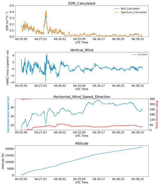
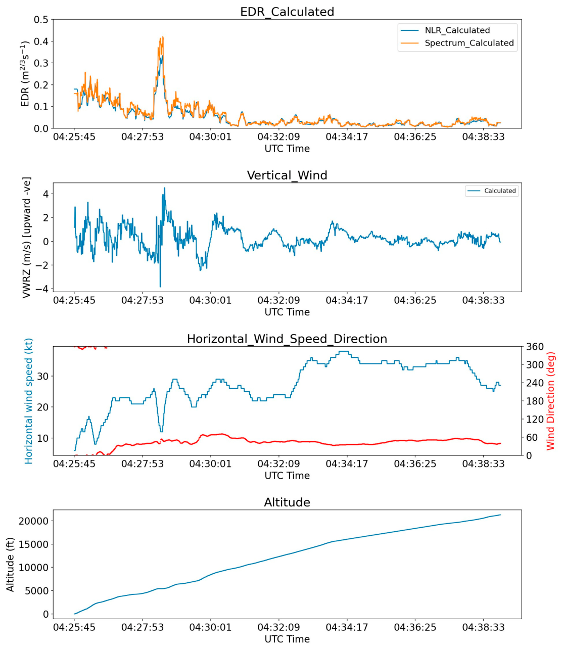
One sample set of evaluated QAR data during Super Typhoon Ragasa is given in Figure 1 for a general illustration of the quality of the meteorological data. The data include the EDR time series, the three components of the wind (horizontal winds in knots, vertical winds in m/s), and the altitude. This was a departing flight at the 07CD corridor; at that time, Ragasa was edging closer to Hong Kong and located about 400 km southeast of Hong Kong. During departure, there was a rapid change in wind speed at around 5500 ft, falling from around 25 to 12 knots and then bouncing back to 25 to 30 knots.
Figure 1.
A sample dataset for the studied aircraft departing from HKIA at 06:25 UTC, 23 September 2025, including EDR, vertical velocity, horizontal wind speed and direction, and altitude of the aircraft.
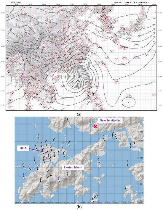
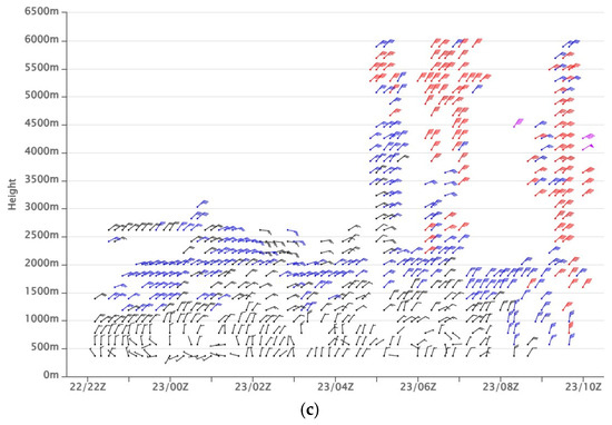
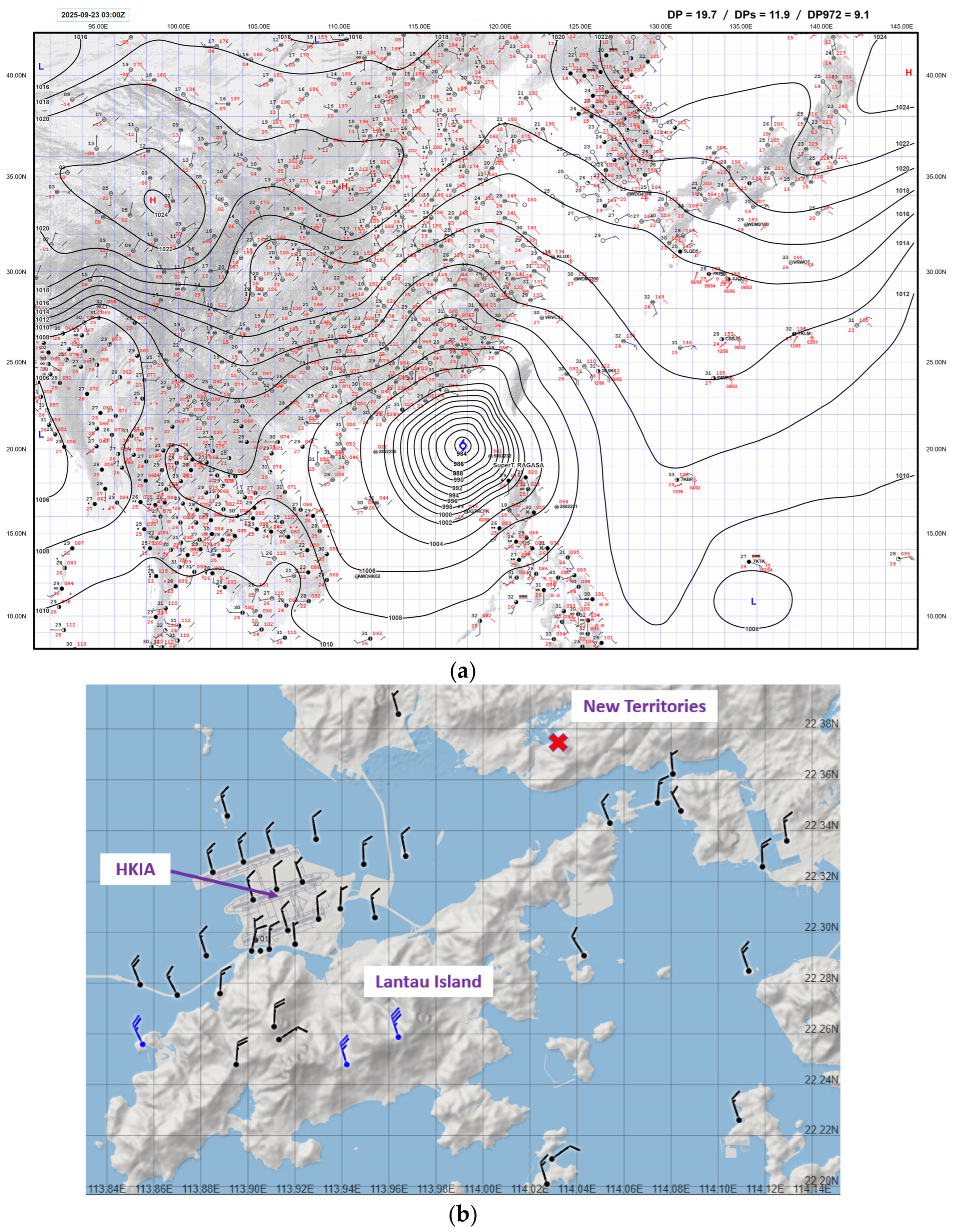
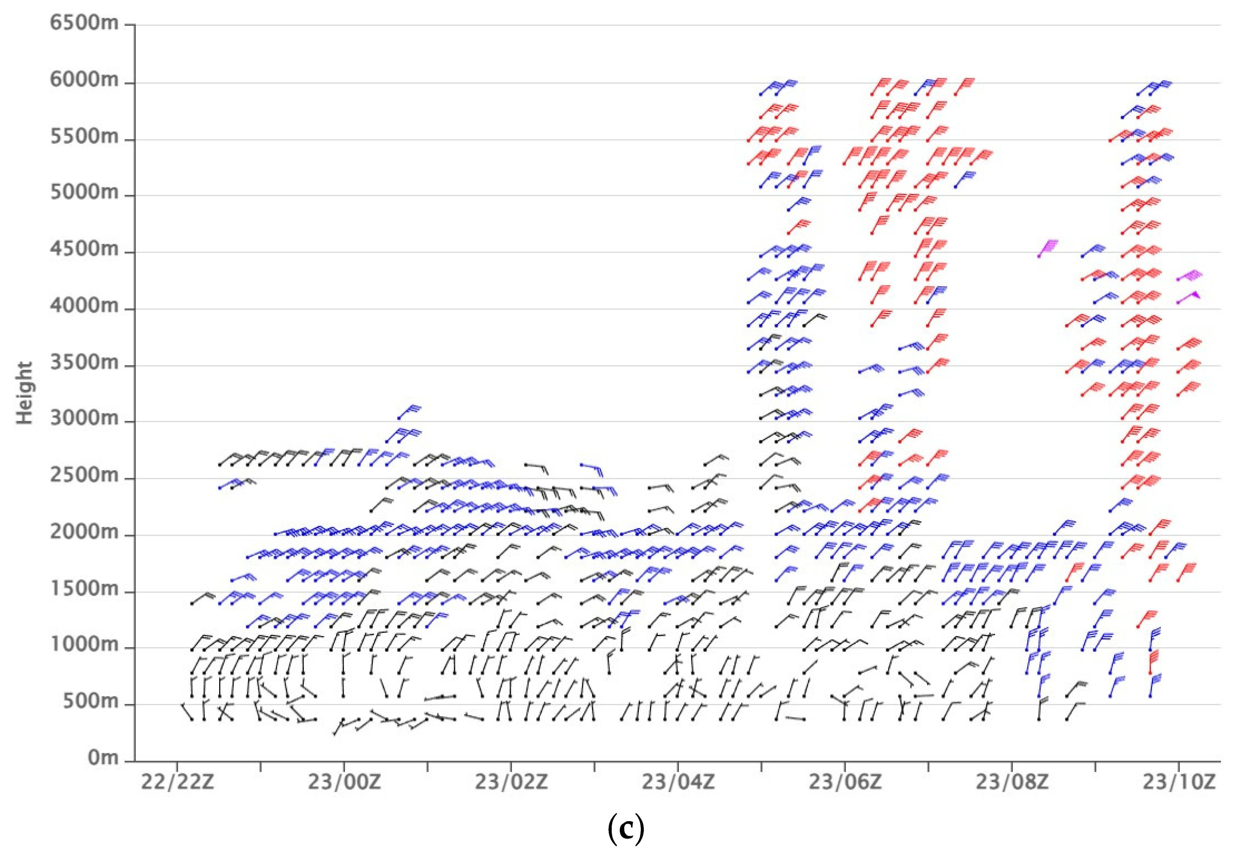
Under the circulation of Ragasa (Figure 2a), moderate north to northwesterly winds prevailed near the surface in the vicinity of HKIA due to sheltering of the terrain, and winds over high ground at Lantau Island reached strong force (Figure 2b), so there was naturally a significant difference in wind speed when the aircraft climbed upwards. The wind profiler at Sha Lo Wan (22.2907° N, 113.8989° E) (Figure 2c) also showed a significant increase in wind speed from 1000 to 2000 m at around 06 UTC. The location at which the rapid change in wind speed occurred was found to be over the terrain over the western part of the New Territories. This was likely related to a pulse in the wind fluctuation in the atmospheric boundary layer of the typhoon, as well as the interaction of the typhoon circulation with the terrain, triggering mountain waves. The vertical velocity fluctuated between +4 and −4 m/s and EDR reached 0.4 m2/3s−1, i.e., moderate turbulence (ICAO [15]). Overall, based on the time series alone, the meteorological data from this flight appear reasonable and comparable with another flight 1 min before this one but using the 07RD corridor (south runway, further away from the terrain to the north), with an EDR of about 0.3 m2/3s−1.
Figure 2.
(a) Surface weather map at 03 UTC on 23 September 2025; (b) the location of the suspected moderate turbulence encounter (marked with a cross and surface wind at 06:25 UTC); (c) Sha Lo Wan wind profiler data at 22 UTC on 22 September 2025 to 10 UTC on 23 September 2025.
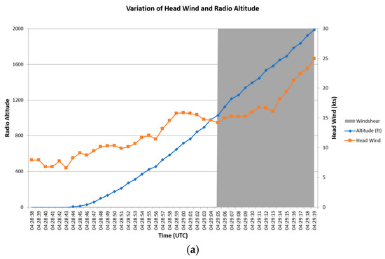
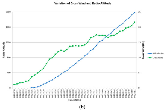
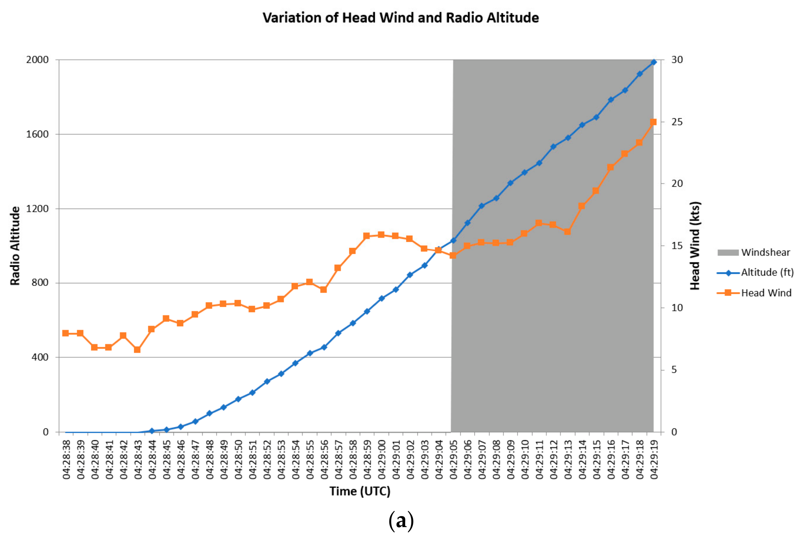
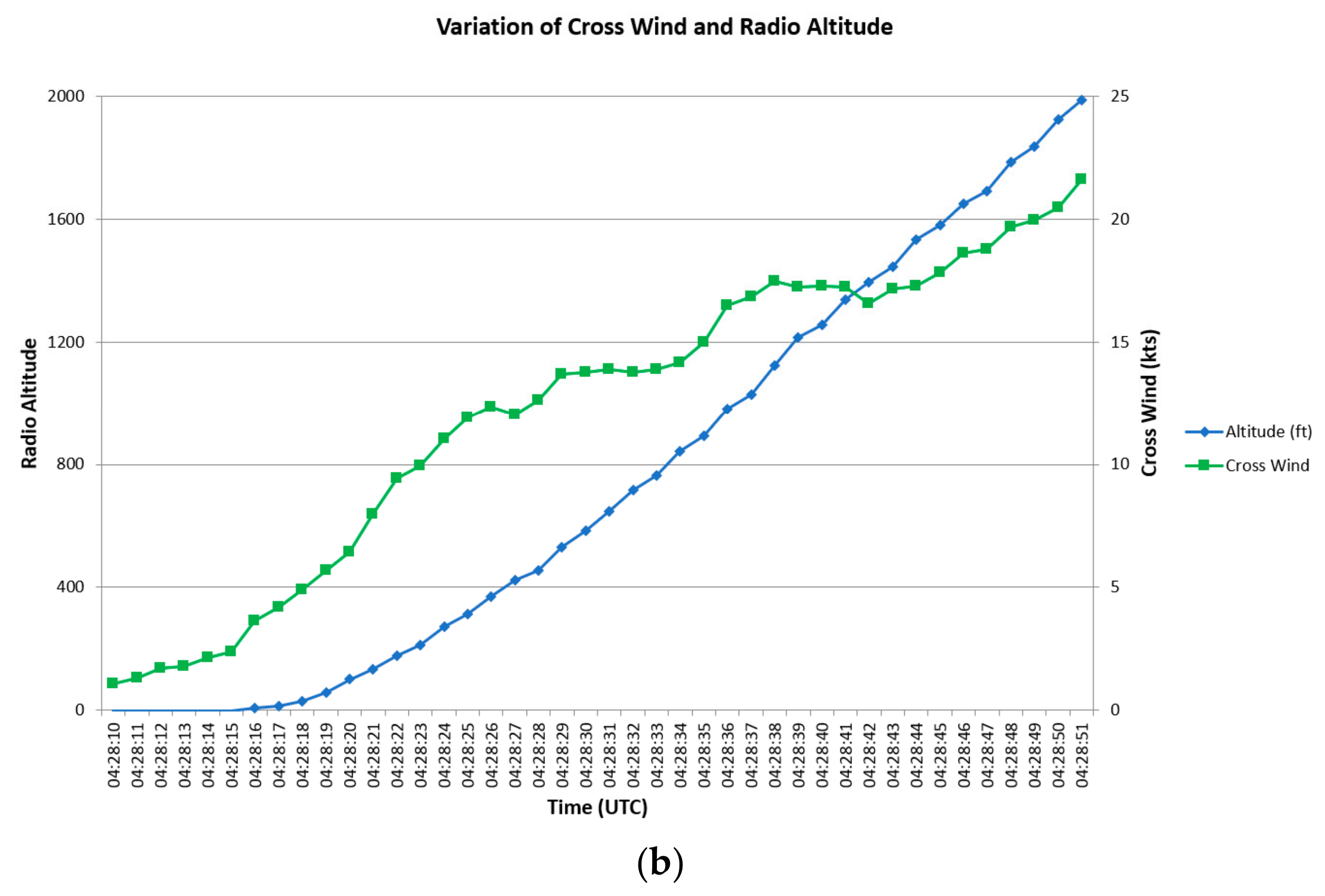
A windshear case following the departure of Ragasa is shown in Figure 3. It was a departure flight from HKIA and both headwind and crosswind increased with altitude. There was a headwind gain of around 11 knots during departure, as highlighted in grey in Figure 3a. Thus, with the quality of meteorological data to be established, data from the studied aircraft type between Hong Kong and Shanghai could be useful for enriching the database of flight data in Hong Kong to further investigate the nature of low-level windshear and turbulence for HKIA and other operating airports.
Figure 3.
(a) Headwind and (b) crosswind profiles for a flight of the studied aircraft type departing from HKIA at 04:28 UTC, 25 September 2025. Windshear is highlighted in grey in (a).
4. Comparison with Low-Level Phase of the Flights
HKIA is located on reclaimed land to the north of Lantau Island, with mountain ranges up to more than 900 m tall, often inducing low-level windshear and turbulence to the airport. In addition, a sea breeze circulation may establish over HKIA under moderate winds and fine conditions, which could also cause a windshear of 20 knots or more at times (HKO [16]). The study of the quality of meteorological measurements at the boundary layer would benefit a future study of these conditions. The low-level phase in this study refers to an altitude up to 2000 feet above sea level. Due to the emphasis on more turbulent flow and the complexity in aligning the flight data from the studied aircraft type with LIDAR data and other flights with available QAR at HKIA for comparison, only the seven flights associated with the typhoon cases of Table 1 are considered. The headwind, crosswind, and EDR of the flights are studied.
For matching with the flight data from a local airline, only flights within 10 min of arrival or departure of the studied aircraft type are considered. To ensure consistency in flight path and atmospheric conditions, the matched flight should use the same runway corridor as the studied aircraft, or at most one runway apart. Consequently, comparison between a flight using the northern runway of HKIA and another using the southern runway is not permitted. For crosswind comparison, we assume that a positive crosswind indicates wind blowing from the right side of the aircraft, and for headwind comparison, we assume that a positive headwind signifies wind blowing against the aircraft.
For matching with the LIDAR, glide-path scans [17] are used to assess headwind profiles up to 2000 feet above sea level, while crosswind profiles are generally not available from LIDAR. The LIDAR scan time needs to be within 3 min of arrival or departure of the studied aircraft. For LIDAR-based EDR analysis, EDR maps derived from the plan position indicator (PPI) scans are utilized [18]. The location of the aircraft is matched with the closest and valid PPI grid point data within an allowance of 300 m, based on PPI scans with an elevation angle of 3.1 degrees for arrival flights and 6.0 degrees for departure flights. The LIDAR PPI EDR time must be within 10 min of arrival or departure of the studied aircraft.
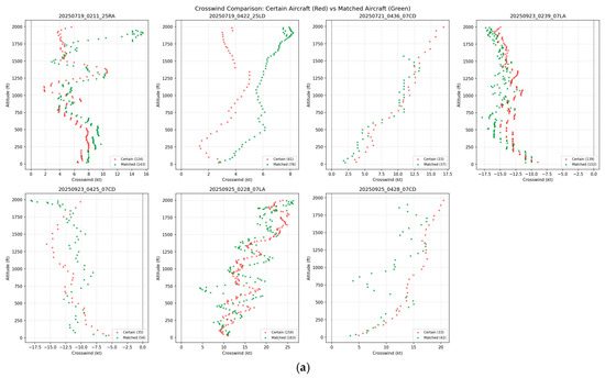
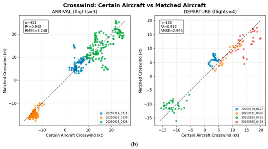
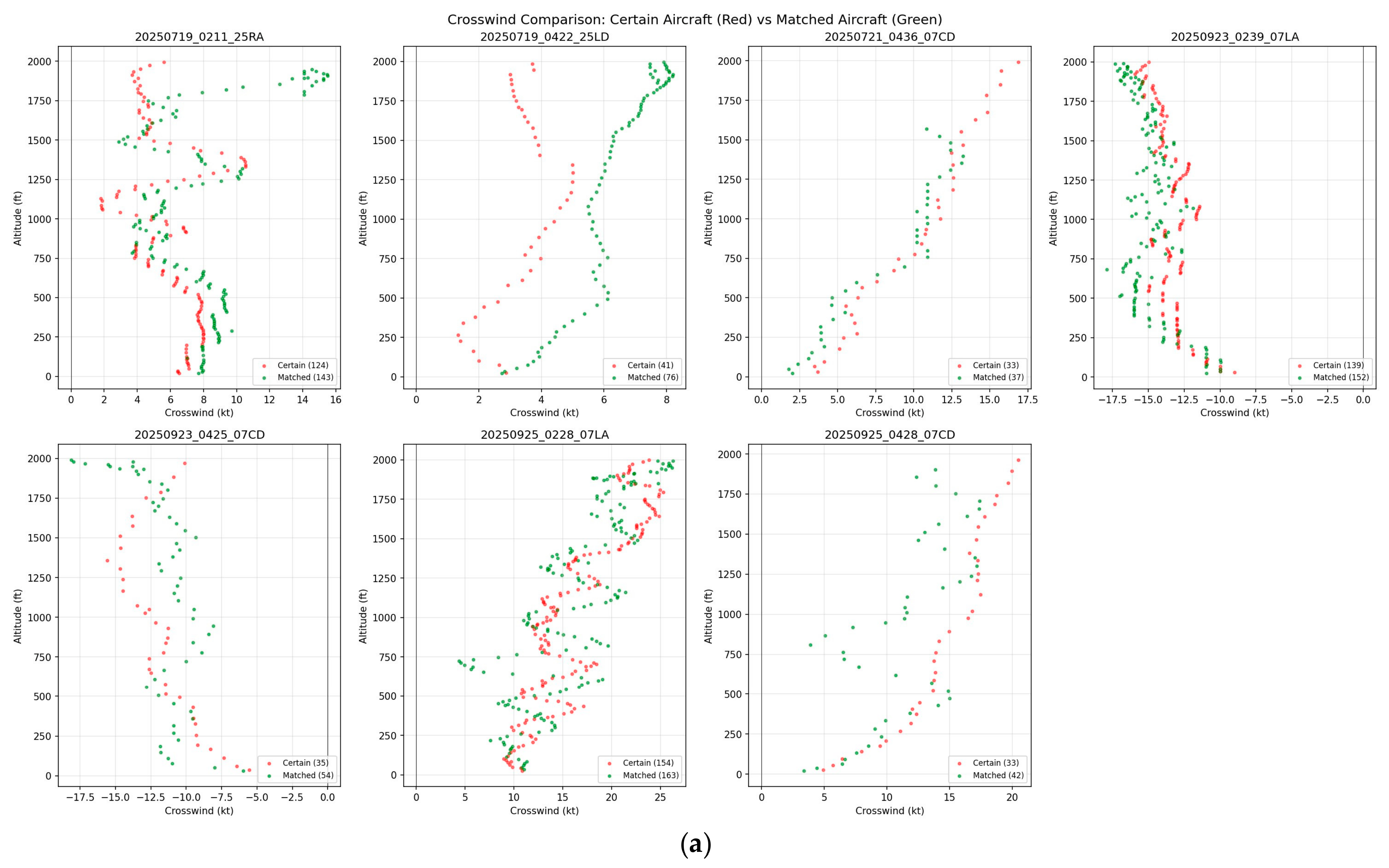
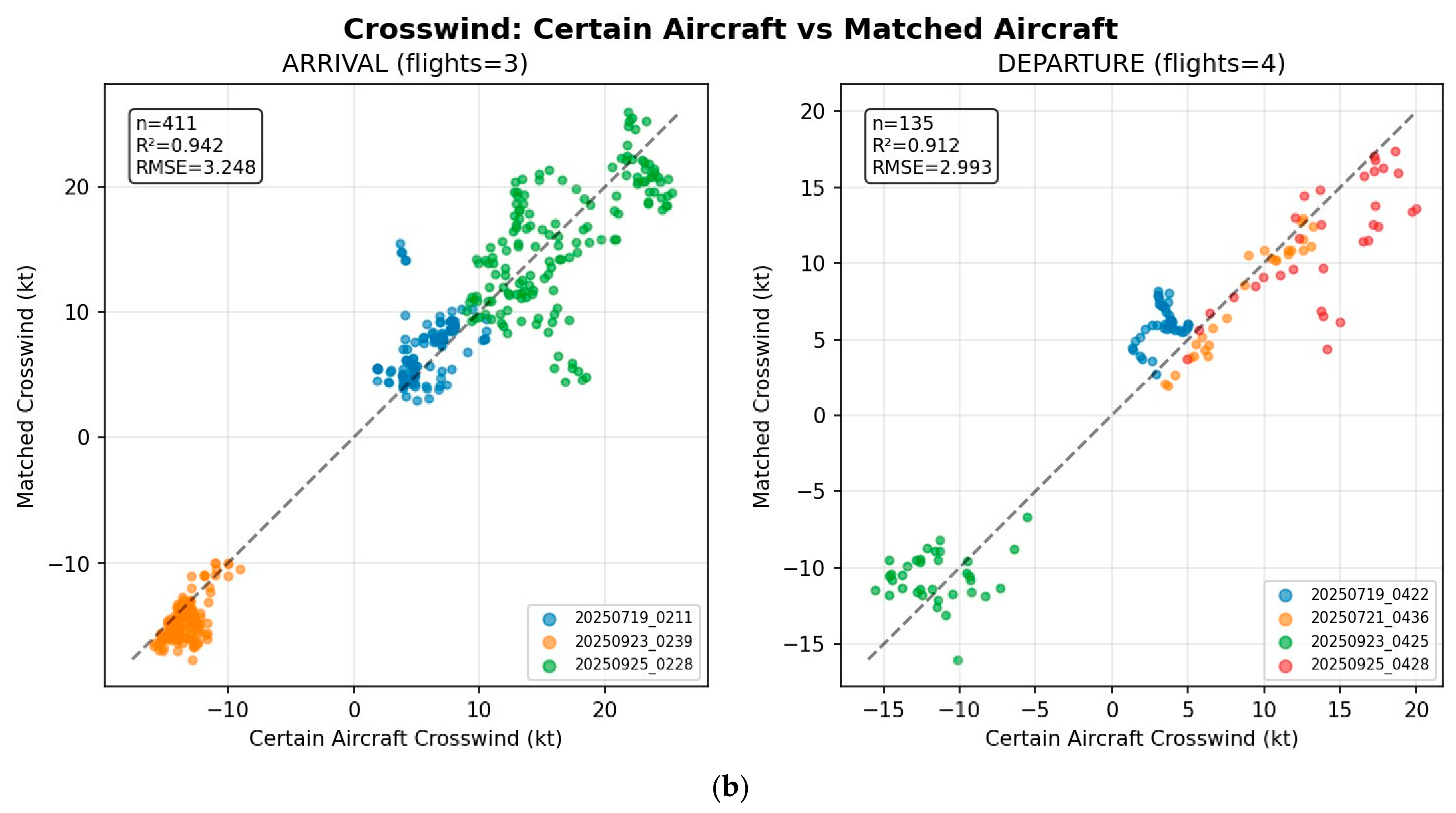
The profiles of the crosswind from the seven flights of the studied aircraft type, together with the matched flights from the local airline, are shown in Figure 4a. Among those flights from the local airline, three are from the A330 family, two from the A350 family, one from the A320 family, and one from the B777 family. It can be seen that there are more data points for arrival flights than departure because departure flights usually climb faster than arrival flights descend, associated with fuel efficiency for departures and the necessity of flow management and safety for arrivals [19]. For arrival flights (the first, fourth, and sixth panels), the trend of crosswinds aligns quite well for the matched aircraft, largely due to the more consistent descending glide paths during approach. By contrast, departure flights exhibit greater variability in crosswinds because differences in take-off locations and climb rate often lead to larger deviations, making direct comparison more difficult. Yet, certain flights (such as the third and fifth panels) still display reasonably good agreement. More quantitative comparison is made through scatter plots in Figure 4b, separated between arrival and departure flights. Though the sample size is small, the crosswinds from the studied aircraft compare very well with those from the local airline. The correlation coefficient squared is of the order of 0.9 and the RMSE is only about 3 knots.
Figure 4.
(a) The vertical profiles of crosswind from the studied aircraft type and the matched flights, and (b) their comparison results in the form of scatter plots.
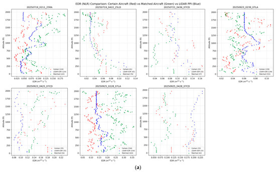
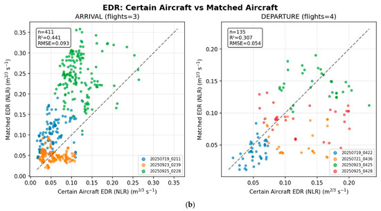
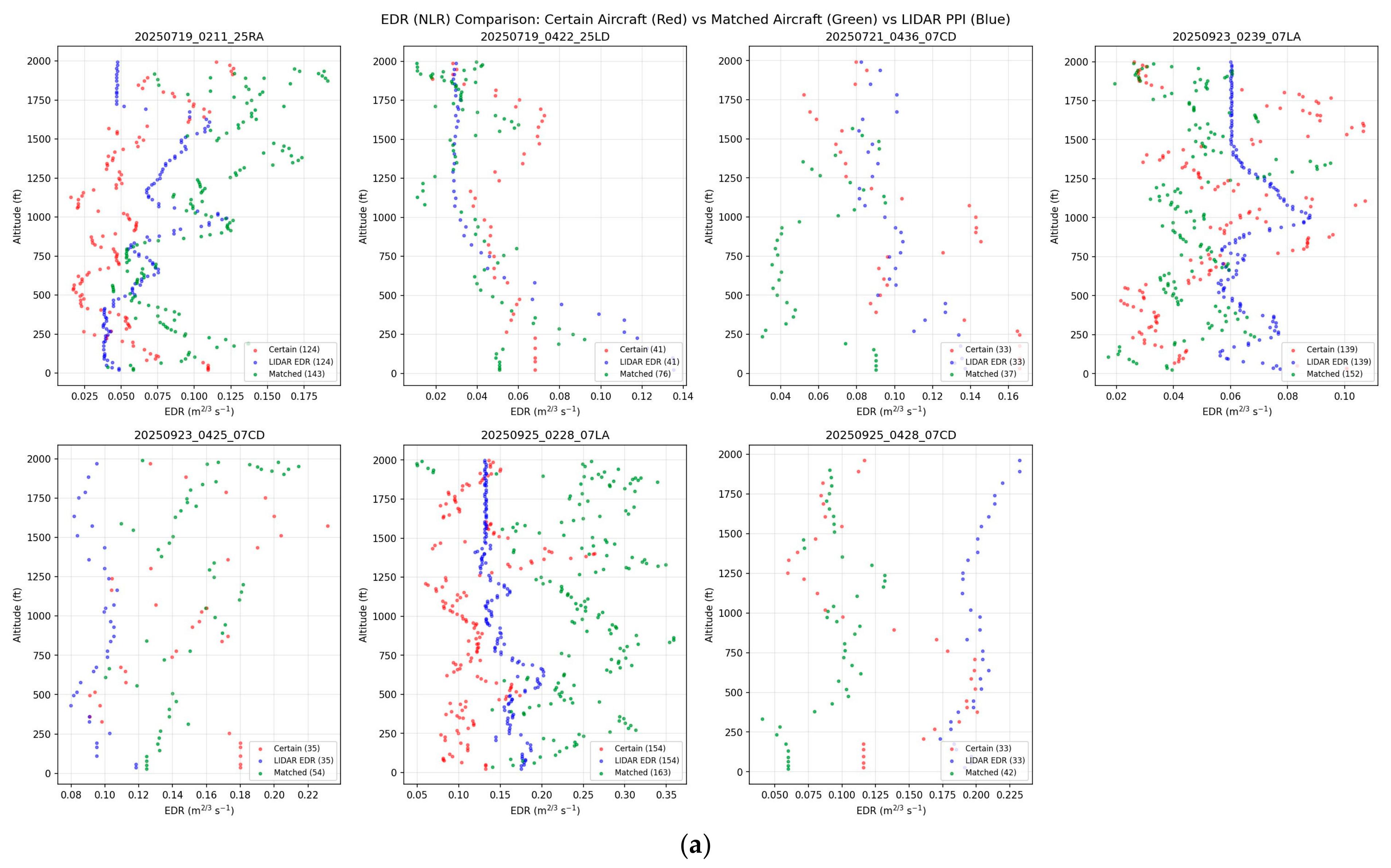
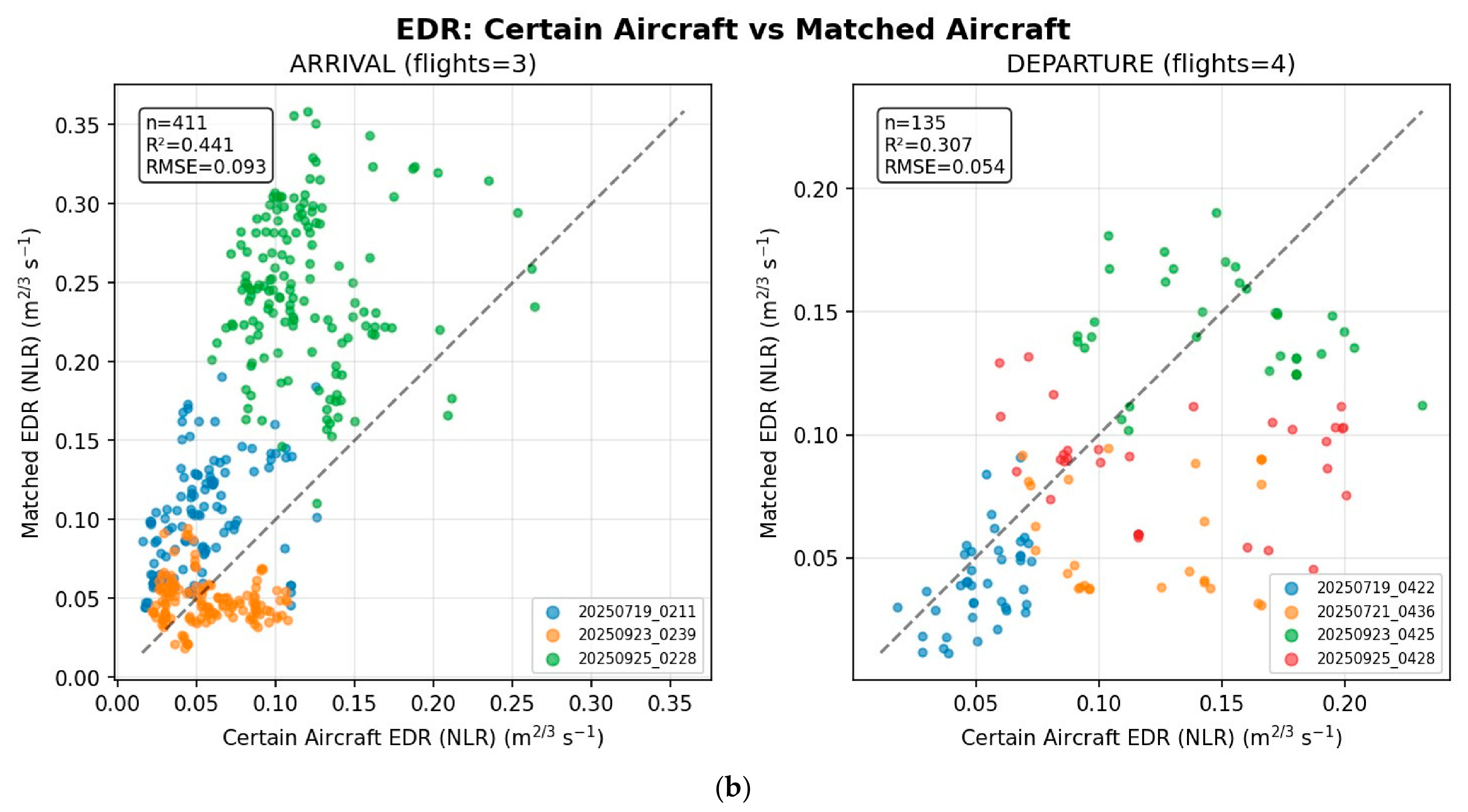
The EDR profiles from the seven flights of the studied aircraft type, the matched flights of the local airline, and LIDAR PPI scans are shown in Figure 5a, and the scatter plots for arrival and departure flights with the matched aircraft are shown in Figure 5b. The direct comparison in the profiles seems to be more dispersed, while in some cases (such as the first and the last panel), there is agreement in the trend of EDR with height but with a shift in magnitude. From the scatter plots, the correlation coefficient squared is of the order of 0.3 to 0.4, but the RMSE is still generally less than 0.1 m2/3s−1, which is of comparable magnitudes. The comparison results for EDR are not as consistent as those for crosswind, because turbulence intensity is highly variable on spatial scales of tens of metres and temporal scales of only a few seconds. The turbulent conditions experienced by the studied flight and the matched flight from the local airline can be quite different even though the temporal difference is within 10 min. Given this, the existing comparison results are considered generally acceptable. It is noted that the data points are closer to the 1:1 line for departure flights than arrival flights. For arrival, the studied aircraft appears to have lower turbulence intensity despite a higher correlation coefficient squared. The results must be validated by more data sources such as subjective pilot reports and guidance of numerical weather prediction models [20,21,22].
Figure 5.
(a) The vertical profiles of EDR from the studied aircraft type, the matched flights, and LIDAR PPI EDR, and (b) the comparison results among aircraft data in the form of scatter plots.
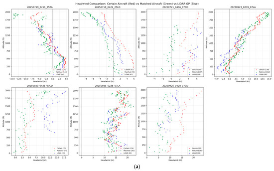
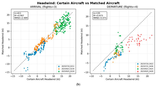
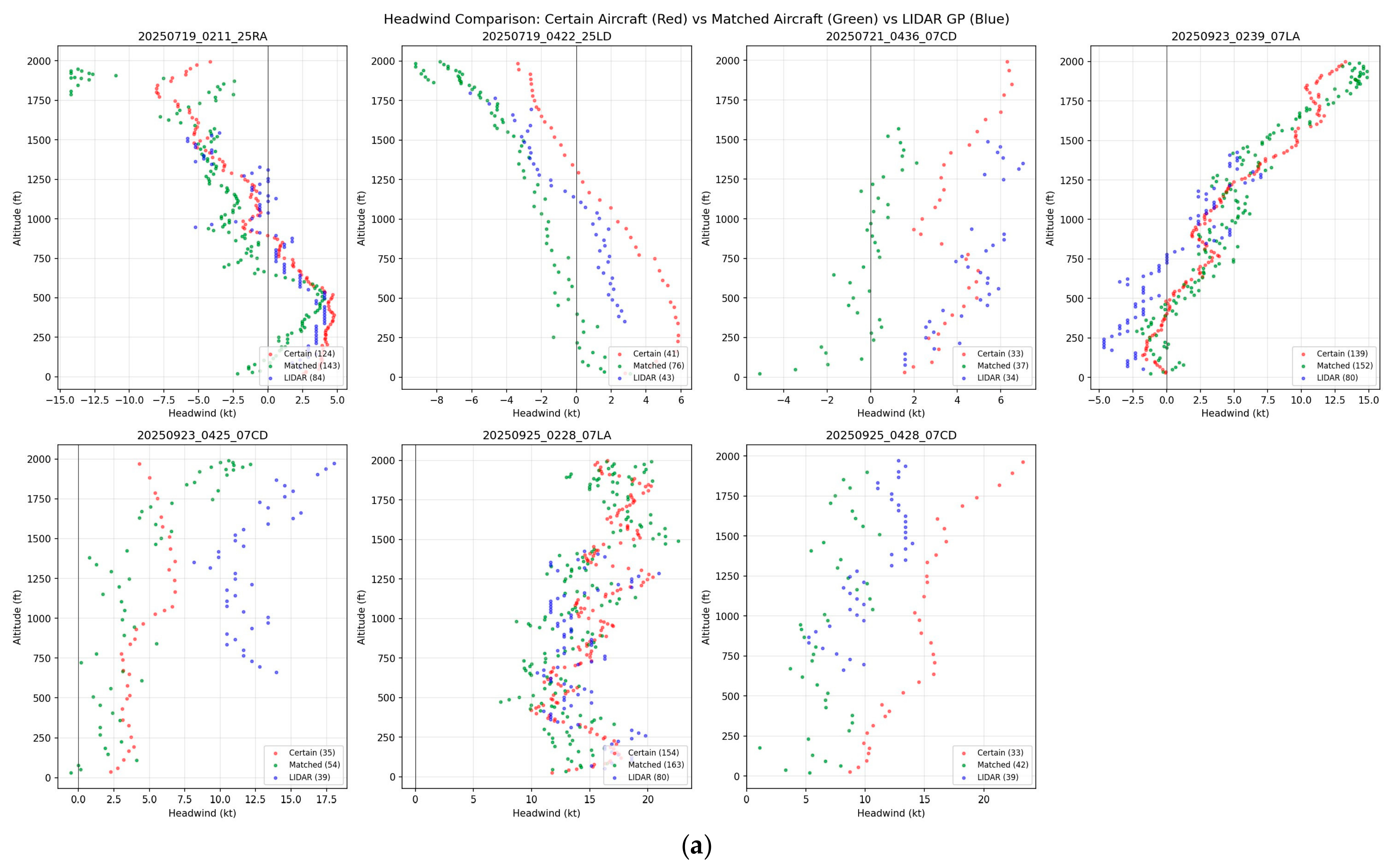
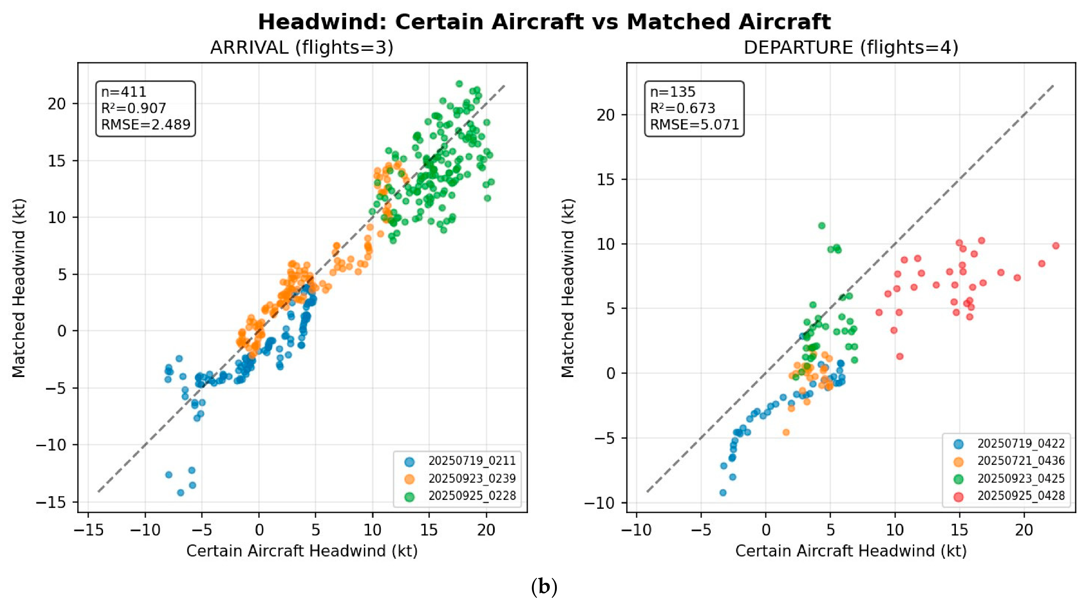
For headwind comparison, the vertical profiles are shown in Figure 6a and the scatter plots are given in Figure 6b. Similar to the crosswind comparison, the headwind comparison is generally satisfactory especially for arrival flights, and the correlation coefficient squared is 0.907 with an RMSE of 2.5 knots. The RMSE for both arrivals and departures is on the order of 2 to 5 knots. The quality of headwind data from the studied aircraft would be sufficiently good for the study of low-level windshear.
Figure 6.
(a) The vertical profiles of headwind from the studied aircraft type, the matched flights, and LIDAR glide-path scans, and (b) the comparison results among aircraft data in the form of scatter plots.
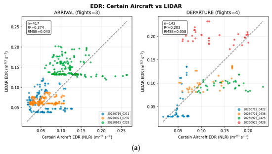
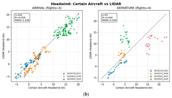
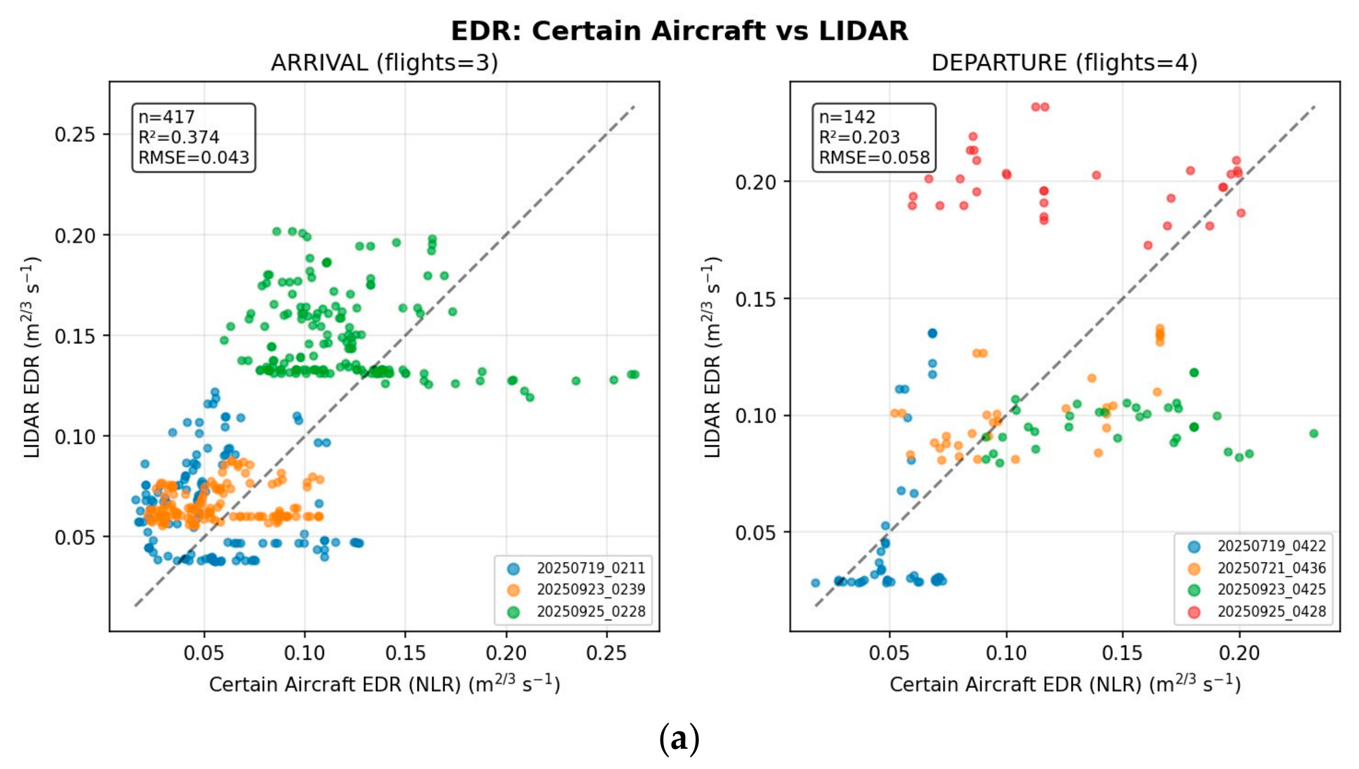
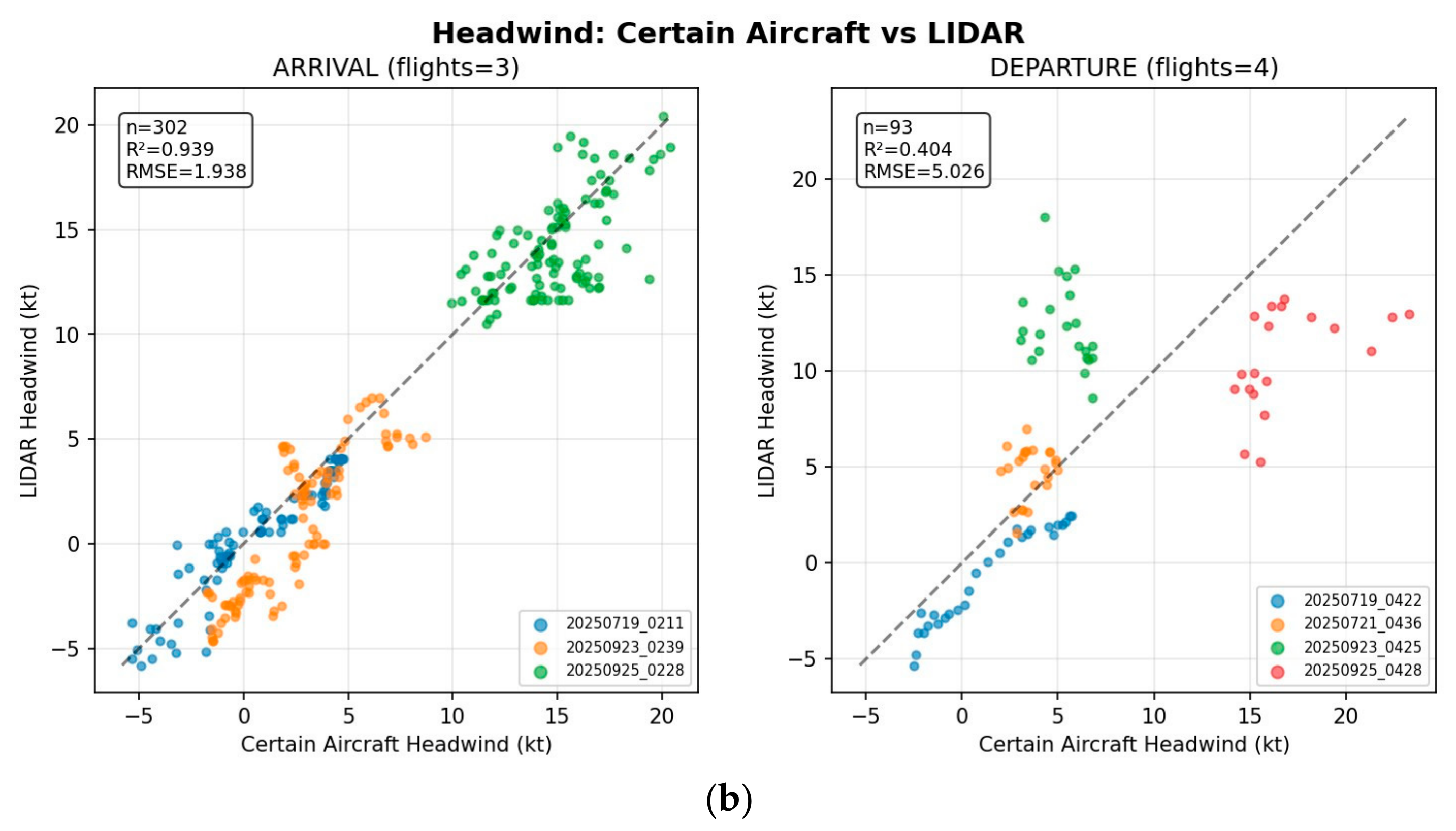
The comparison results with LIDAR are shown in Figure 7, namely, EDR in Figure 7a and headwind in Figure 7b. For EDR, the under-reading of EDR for the studied aircraft does not seem to be present when compared with the LIDAR-derived EDR. The RMSE is generally less than 0.06 m2/3s−1. However, it is noticed that the spread of EDR is large in the scatter plot with a lower correlation coefficient squared, which also reflects the sporadic and instantaneous nature of turbulence. For headwind, the comparison is good with a correlation coefficient squared up to 0.939 for arrival flights, and an RMSE below 2 knots. The discrepancy for departure flights could be attributed to the variability in glide path as discussed in the cases of crosswinds.
Figure 7.
Comparison between the studied aircraft type and LIDAR data for (a) EDR and (b) headwind for the 7 flights of this aircraft.
It must be emphasized that the present comparison is based on a limited sample in the typhoon situation. The quality of horizontal wind speed and direction measured by the studied aircraft between Hong Kong and Shanghai is discussed below with a more generalized dataset; however, there is a lack of objective measurements of enroute EDR to compare with at this stage.
5. Comparison with Enroute Phase of the Flights
The quality of horizontal wind speed and wind direction in the QAR data of the certain aircraft type during the enroute phase between Hong Kong and Shanghai is evaluated by comparing with the ERA5 reanalysis data from ECMWF. The dataset comprises 151 flights from July to September 2025, providing a sufficient sample size for more robust and generalized comparison results. In the enroute comparison, altitudes are stratified into three levels at or above 2000 feet to minimize boundary layer effects: 2000–8000 feet (low level), 8001–20,000 feet (medium level), and above 20,000 feet (upper level). This stratification enables an objective comparison of wind speed and direction across different flight stages, with more maneuvering at the two lower levels and relatively stable cruising at the uppermost level. For wind direction comparisons, a minimum wind speed of 10 knots is required to reduce the random variability associated with lighter winds.
For spatial (horizontal) matching, the ERA5 reanalysis data, which is structured on a regular 0.25° × 0.25° grid, is paired with the QAR data by identifying the nearest ERA5 grid point using Euclidean distance for each QAR point. The search radius is limited to 0.5° (approximately 55 km) to prevent matching with distant points. Interpolation is not performed, as a positional accuracy of around 10–20 km is deemed sufficient for enroute conditions.
For vertical matching, the QAR altitude (in feet) is first converted to pressure (in hPa) using the barometric formula as flights employ barometric altitude. At each matched grid point, the two nearest ERA5 pressure levels are identified, and linear interpolation is applied to estimate wind conditions at the exact QAR altitude. Matches are rejected if the QAR and ERA5 altitudes differ beyond the following tolerances: 800 feet at the lower level, 1200 feet at mid level, and 2500 feet at upper level.
For temporal matching, the QAR data, sampled every 20 s, are mapped to the ERA5 hourly averaged wind data to the nearest hour, because ERA5 wind data is available on an hourly basis (00:00, 01:00, … up to 23:00 UTC).
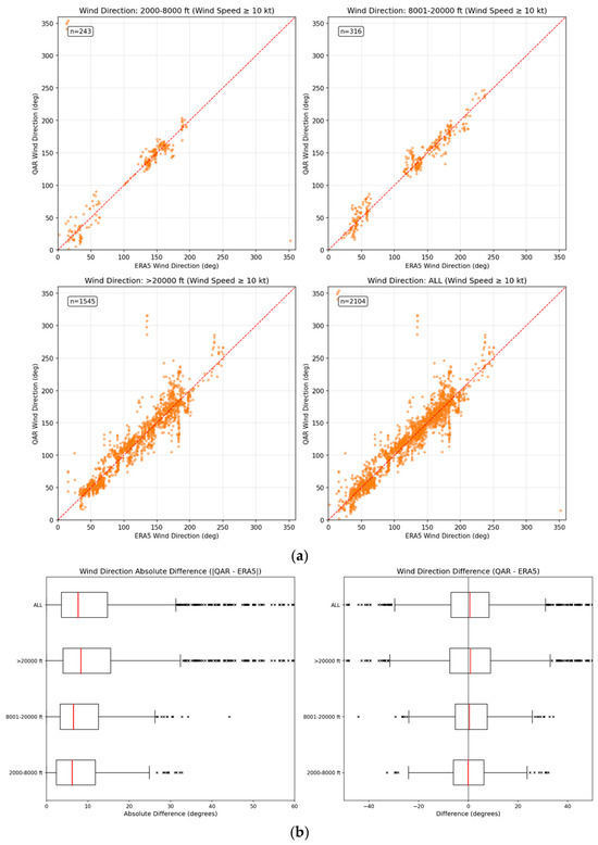
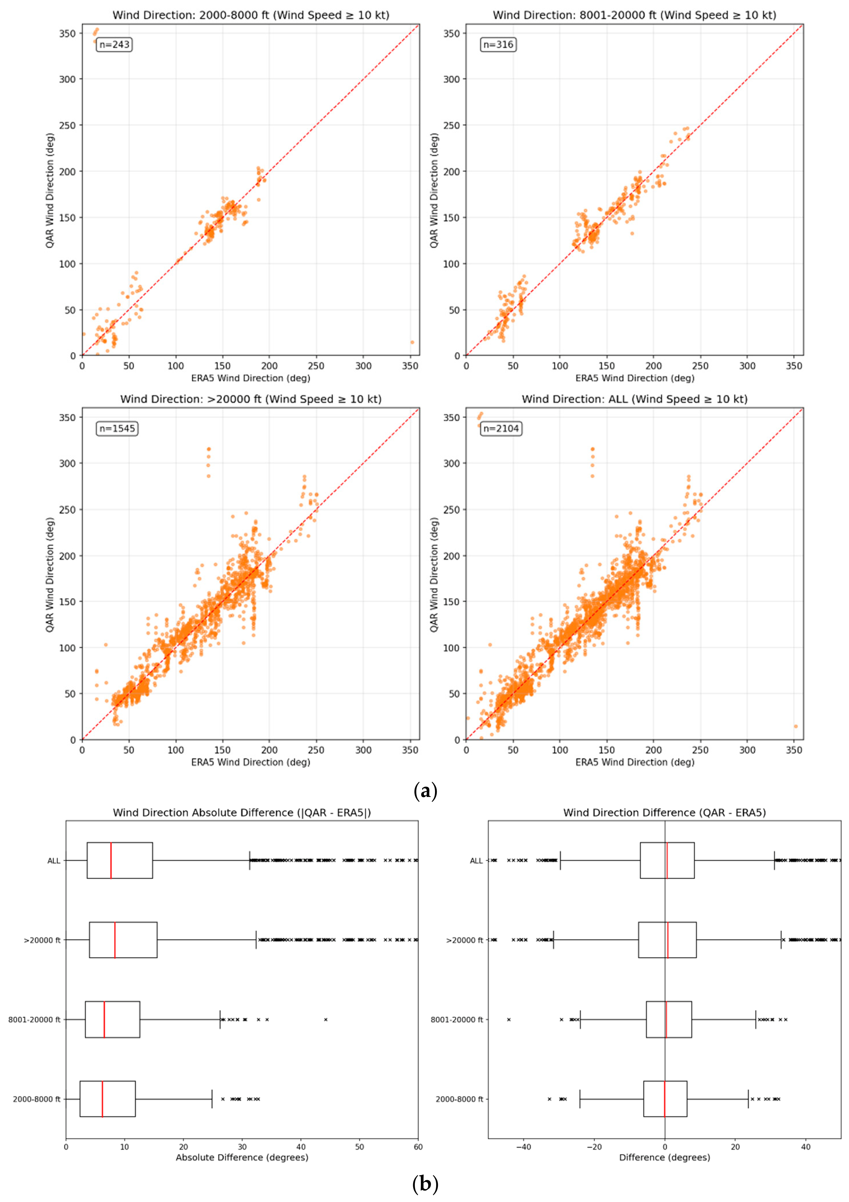
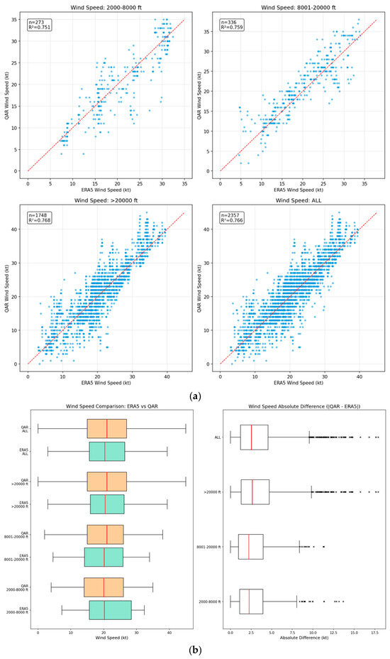
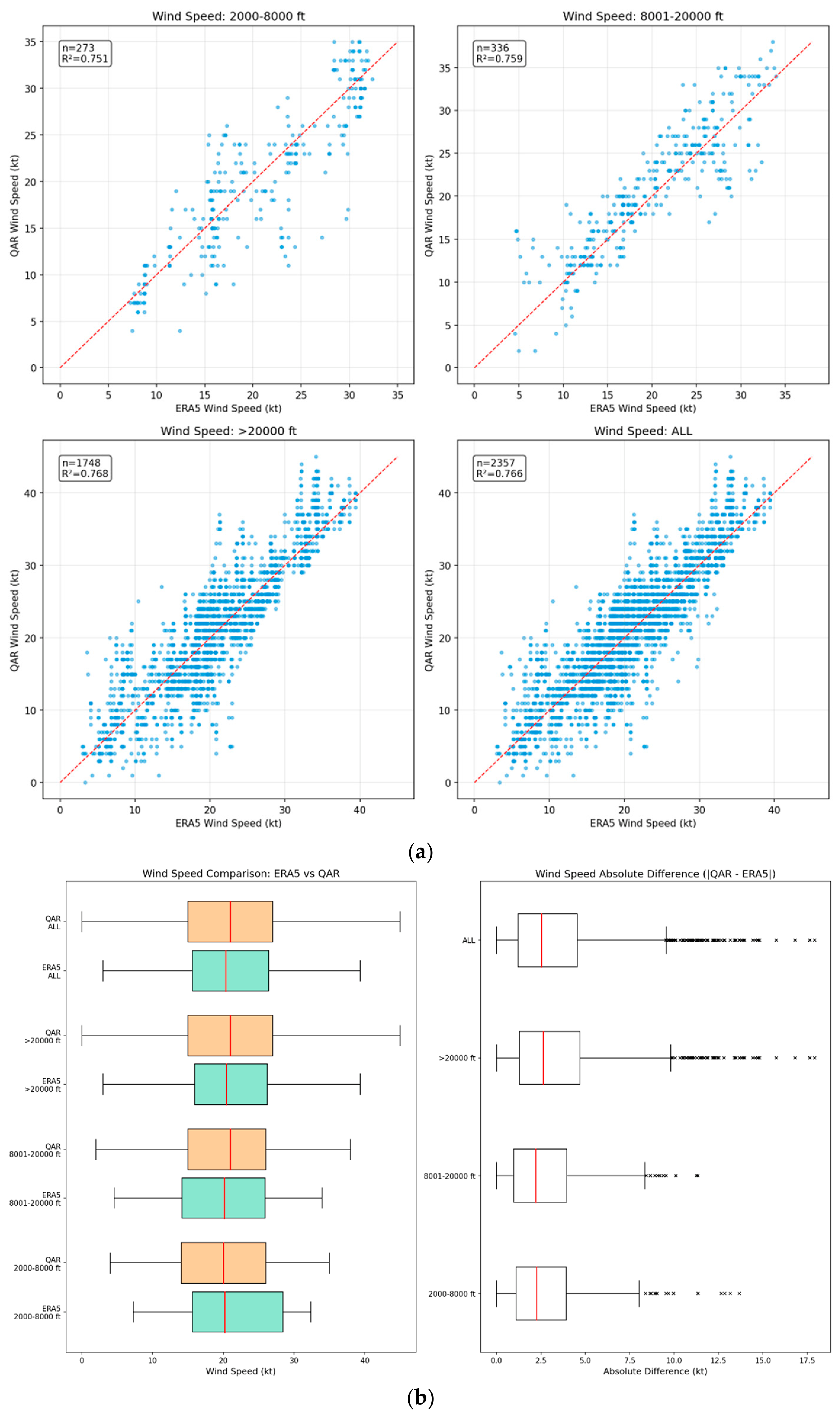
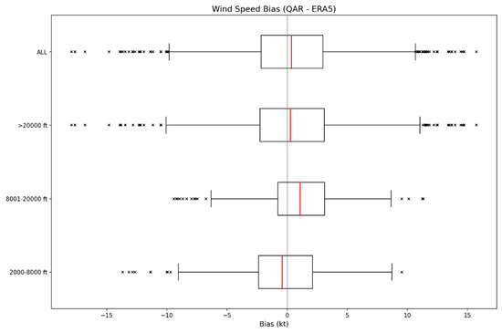
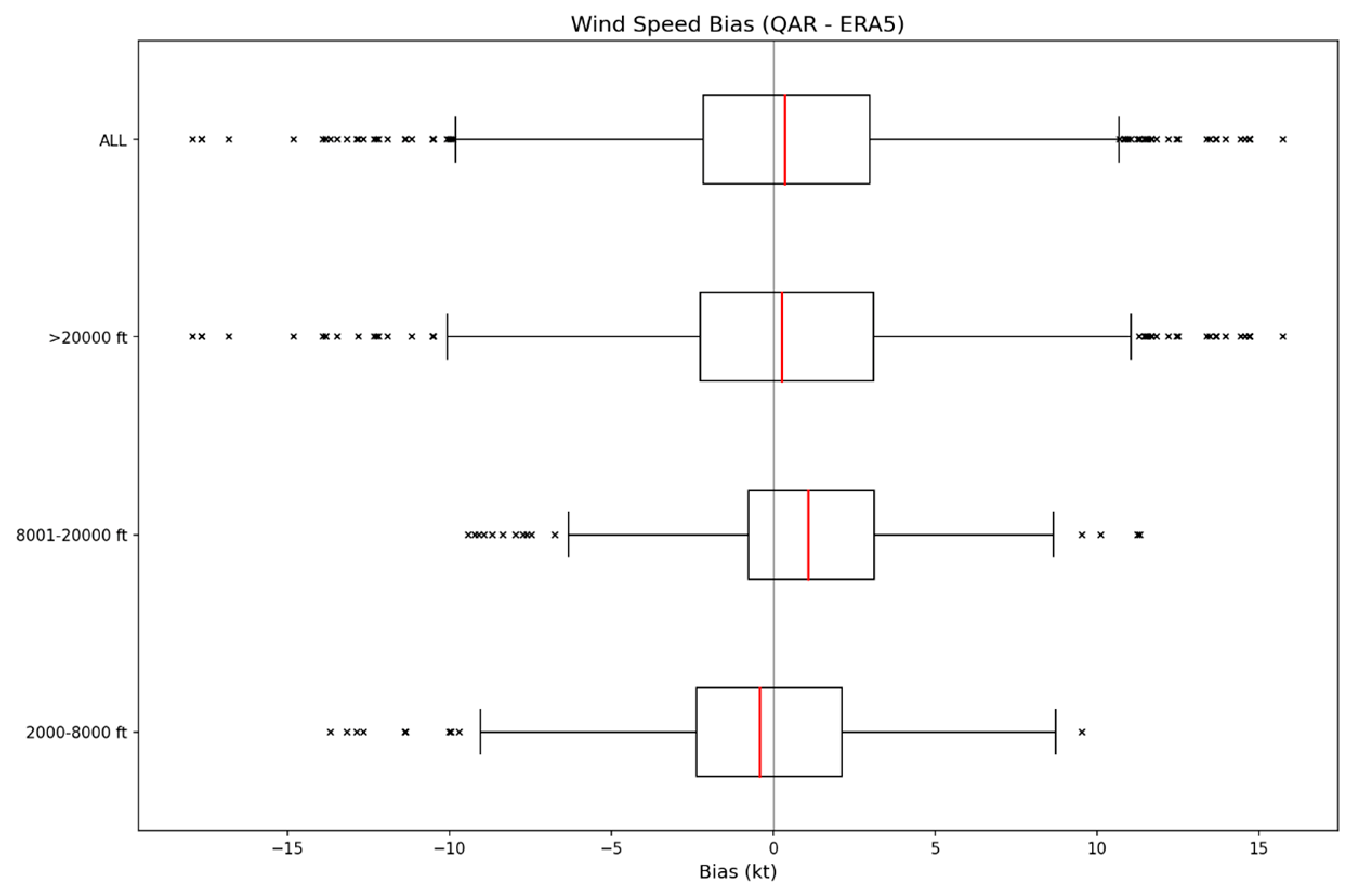
The comparison results for the seven flights as given in Table 1 are first presented. There are 2357 valid data points in total, of which 273, 336, and 1748 correspond to the low, medium, and upper levels. The wind direction comparison results are shown in Figure 8, the scatter plots at various height stratifications in Figure 8a, and the mean absolute difference and the mean difference (bias) in Figure 8b as box and whisker diagrams. The scatter plots show that the two datasets are in good agreement. The 50th and 75th percentiles of mean absolute difference for all levels are 7.6 and 14.7 degrees, respectively, and the bias is close to zero degrees. The wind speed comparison results are shown in Figure 9. In various height stratifications, the correlation coefficient squared is within 0.75 to 0.80, as shown in Figure 9a. This is again reflected in the box and whisker diagrams of the spreading of the wind speeds of the two datasets (left hand side of Figure 9b). The mean absolute differences are generally within 5 knots (right hand side of Figure 9b). The bias between the two datasets is shown in Figure 10 and it is found to be close to zero knots for most cases. As such, for the limited dataset in the two typhoon situations, the horizontal wind speed and wind direction from the QAR of the studied aircraft type appear to be comparable with those from the reanalysis of the numerical weather prediction model.
Figure 8.
(a) Scatter plots of wind direction comparison between QAR and ERA5 for various height ranges; (b) box-and-whisker diagrams of absolute difference (left) and difference showing the bias (right).
Figure 9.
(a) Scatter plots of wind speeds from QAR and ERA5 for various height ranges, and (b) box-and-whisker diagrams of the spreading of wind speed (left) and the spreading of absolute difference (right).
Figure 10.
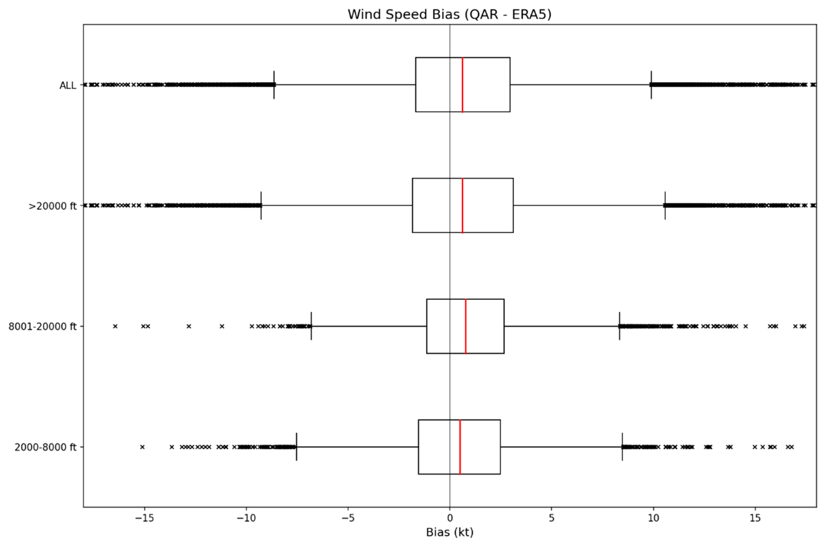
The wind speed bias of QAR data with respect to ERA5 for various height stratifications.
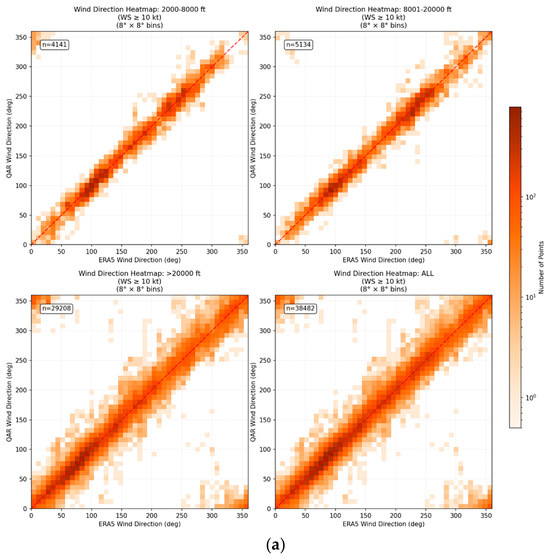
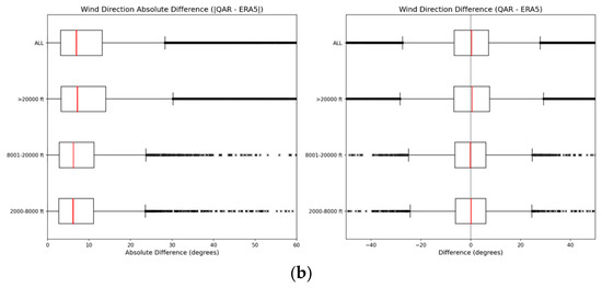
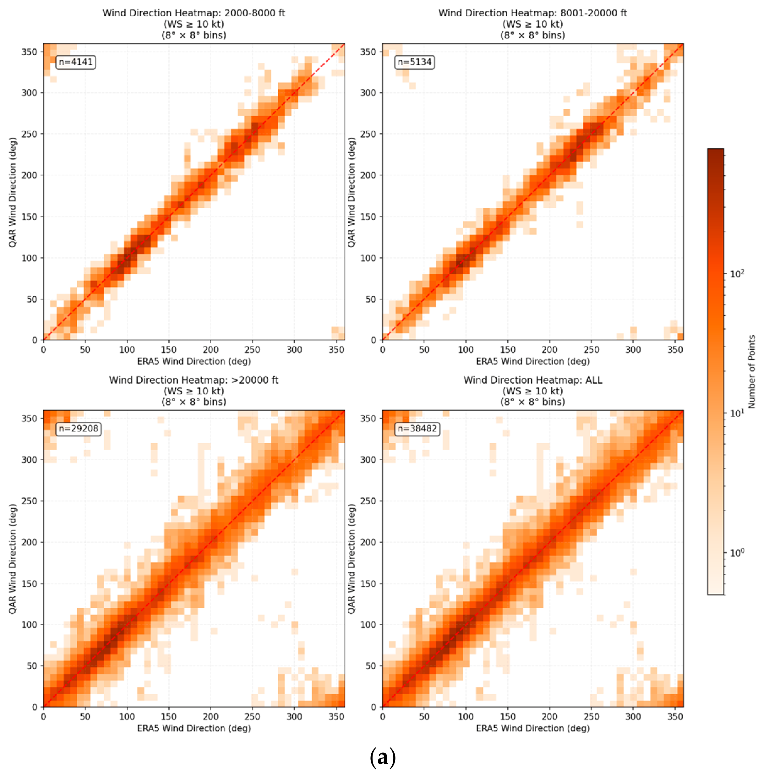
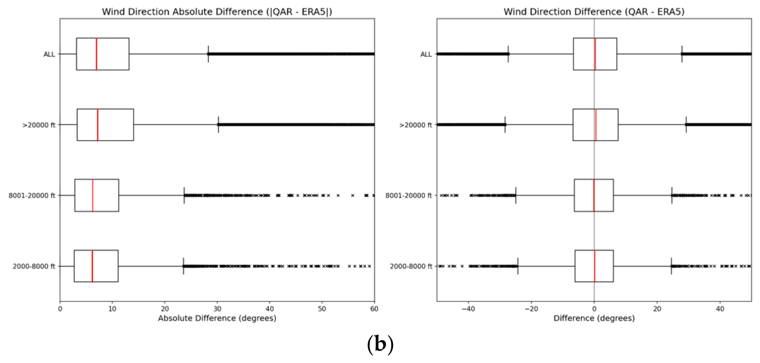
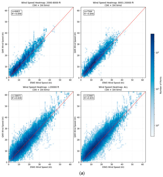
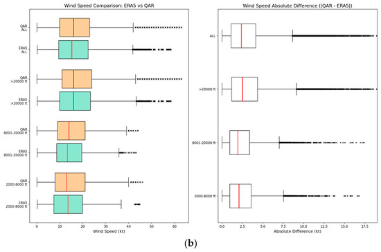
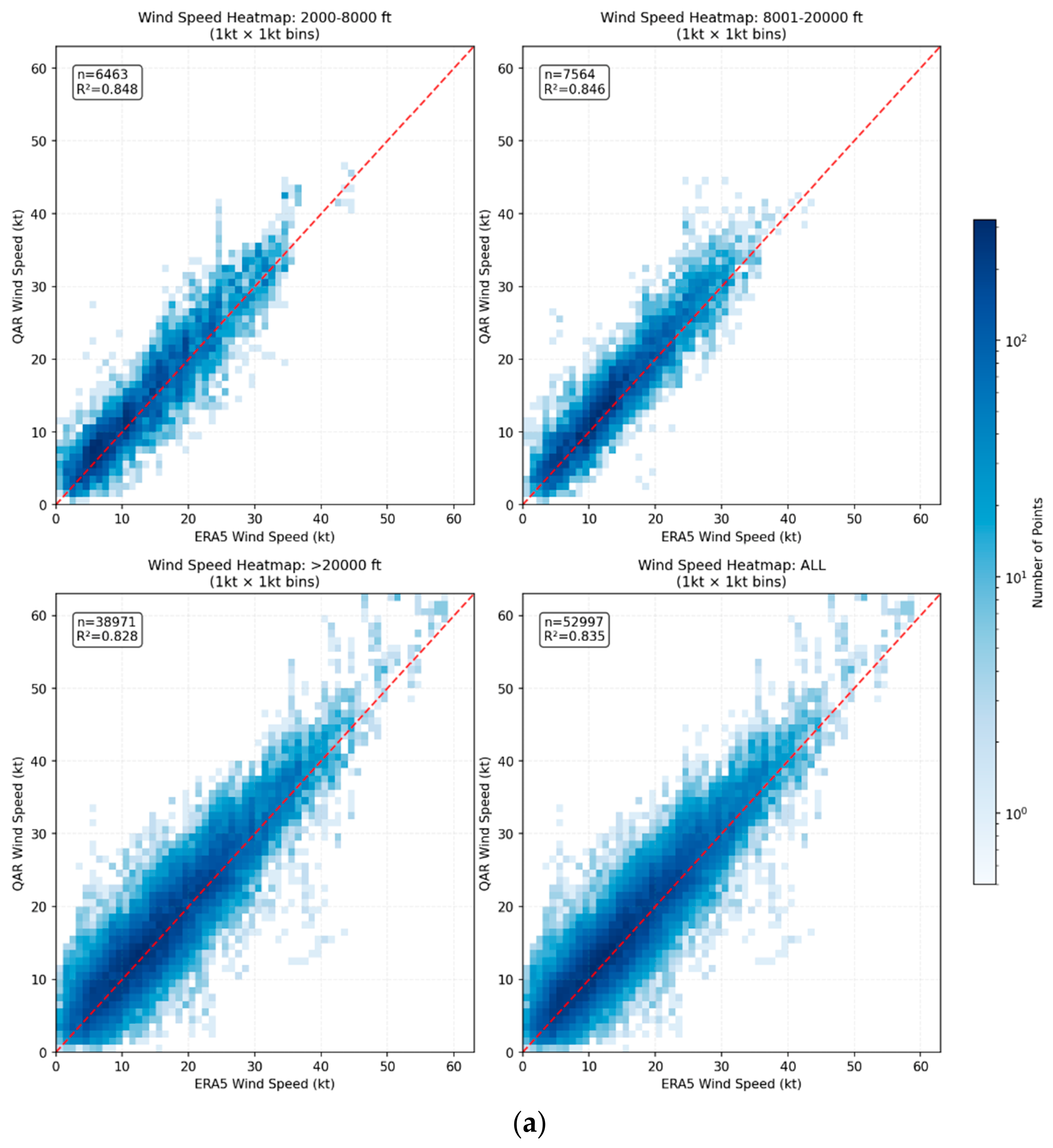
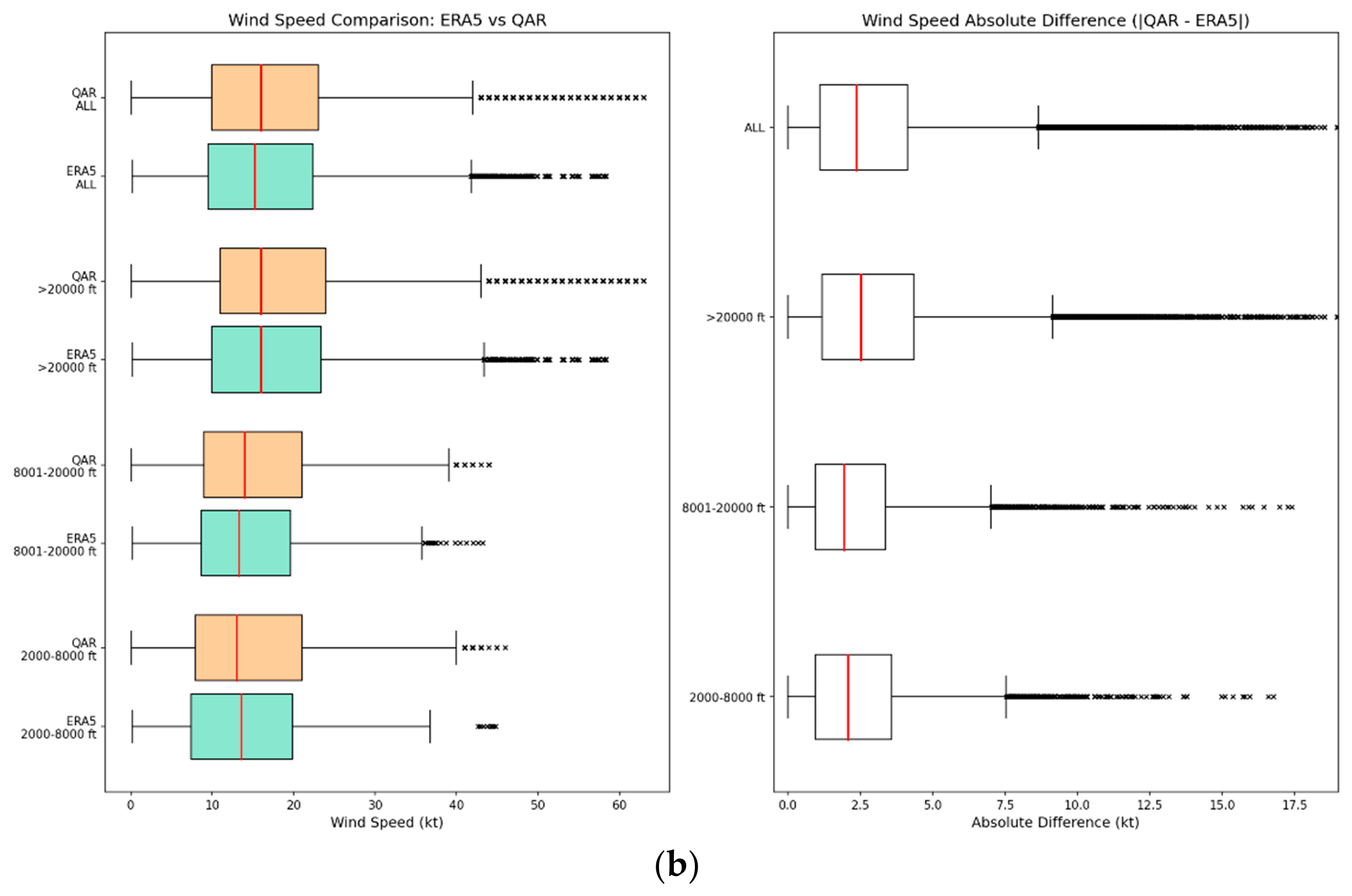
In the extended dataset covering July and September 2025, there are 151 flights and 52,997 data points in total, in which 6462, 7564, and 38,971 are from the low, medium, and upper levels, respectively. The scatter plots of the two datasets for wind direction and wind speed are shown in Figure 11a and Figure 12a, respectively, in the form of heat maps. The correlation coefficient squared for wind speed is found to be in the region of 0.8 for the various height stratifications. As shown in Figure 11b, the absolute difference in wind direction for the two datasets is mostly in the region of 5 to 15 degrees, and the bias is close to zero degrees at the various height ranges. Figure 12b shows the spreading of wind speed from the two datasets for different height ranges, and the spreads appear to be similar. The absolute difference in Figure 12b is mostly below 5 knots, indicating that the datasets are generally comparable. The bias diagram for wind speed in Figure 13 shows there is a slight positive bias of about 1 knot on average for the QAR data with respect to the reanalysis data at various altitude ranges.
Figure 11.
Wind direction for the enroute phase of the studied aircraft type between July and September 2025: scatter plots in the form of heat maps for various height ranges in (a), and box-and-whisker diagrams for the spread of the absolute difference and difference between QAR and ERA5 reanalysis data in (b).
Figure 12.
Comparison of wind speed between QAR and ERA5 reanalysis data between July and September 2025: (a) scatter plots in the form of heat maps for various height ranges; (b) box-and-whisker plots of the spread of wind speed and absolute difference.
Figure 13.
Bias of QAR wind speed with respect to ERA5 reanalysis data for the period from July to September 2025.
The comparison results for wind direction and wind speed are summarized in Table 2 and Table 3, respectively, which may serve as indications of the accuracy level of the horizontal wind speed and wind direction from the QAR data based on the current dataset. In the interpretation of comparison results, it is worth understanding that the ERA5 wind is 1 h averaged and gridded, while QAR data is instantaneous and point-based spatially. As such, the QAR data are considered to have satisfactory quality given a correlation coefficient squared of about 0.8, generally negligible bias, and relatively small mean absolute difference.
Table 2.
The 50th and 75th percentiles of absolute difference and the 25th, 50th, and 75th percentiles of bias for wind direction (≥10 knots) (degree) at various altitude ranges in the 3-monthly comparison.
Table 3.
The 50th and 75th percentiles of absolute difference and the 25th, 50th, and 75th percentiles of bias for wind speed (knot) at various altitude ranges in the 3-monthly comparison.
6. Conclusions
The quality of wind measurements made onboard a certain type of commercial aircraft manufactured in China is studied for the first time in the literature through extensive comparison with other data sources, namely, data from other fleets before and after the concerned flights, independent measurements from ground-based Doppler LIDARs, and ERA5 reanalysis. The winds and related parameters from QAR data, including the headwind and crosswind up to 2000 feet, or the horizontal wind speed and wind direction at or above 2000 feet, are found to have generally satisfactory quality through the various comparisons. The comparison for EDR also has a relatively small RMSE, but the correlation is relatively weak due to the sporadic and instantaneous nature of turbulence, even when compared with objective data sources. Due to the variability in turbulence, the comparison results of EDR are still considered acceptable. The wind parameters from the QAR of the studied aircraft type and the independent measurements are, in general, well correlated. The horizontal wind speed and wind direction, including the headwind and crosswind derived, compare particularly well with the other measurements, and such data could be useful for the study of windshear as well as data assimilation into numerical weather prediction models. However, the temperature comparisons are not presented in this paper, as wind fields are generally smoother at cruise level as a result of synoptic dynamics, except under convections or waves. In addition, ground-based remote sensing measurements of temperature, such as those from radiometers, are usually taken in the vertical direction only, while the aircraft may be located tens of kilometres away from the observed column. A fairer comparison would require temperature measurements from multiple sensors installed on the aircraft.
For the low-level comparisons below 2000 feet, the present study is conducted based on a limited sample of seven flights during typhoon conditions only, and a much larger dataset would be needed to establish the quantitative accuracy of low-level wind and EDR from the studied aircraft type. In particular, data of this aircraft in more cases of low-level windshear and turbulence at HKIA would need to be collected. For the enroute phase, the comparison only covers a period of three months. The data quality in other seasons of the year would need to be analyzed to understand the quality of measurement under different weather systems, say, the westerly jet stream at mid to upper levels in winter. It would also be interesting to see how the enroute EDR behaves and whether they are consistent with other assessments of turbulence, such as clear air turbulence products from major aviation meteorological centres. In summary, more meteorological conditions and larger datasets would be required so that the quality of wind-related parameters measured by this aircraft type could be much better established.
Supplementary Materials
The following supporting information can be downloaded at https://www.mdpi.com/article/10.3390/app16136482/s1, Figure S1. Arrival corridors of HKIA and the location of LIDARS (marked with yellow dots).
Author Contributions
Conceptualization, P.W.C.; methodology, P.W.C.; software, M.L.C.; validation, M.L.C.; formal analysis, M.L.C.; investigation, M.L.C. and D.W.; data curation, D.W. and P.W.C.; writing—original draft preparation, P.W.C.; writing—review and editing, D.W. All authors have read and agreed to the published version of the manuscript.
Funding
This research received no external funding.
Institutional Review Board Statement
Not applicable.
Informed Consent Statement
Not applicable.
Data Availability Statement
The datasets presented in this article are not readily available, because the data will be used for internal analysis under a non-disclosure agreement and flight data are not available for other parties.
Acknowledgments
The authors would like to acknowledge the help of Junying SUN and Yangjinxi GE of COMAC Meteorological Research Center, Shanghai Aircraft Flight Test Co., Ltd., Shanghai, for the provision of the aircraft data for the new flight route between Hong Kong and Shanghai for the study.
Conflicts of Interest
The authors declare no conflicts of interest.
References
- Moninger, W.R.; Mamrosh, R.D.; Pauley, P.M. Automated meteorological reports from commercial aircraft. Bull. Am. Meteorol. Soc. 2003, 84, 203–216. [Google Scholar] [CrossRef] [Scilit]
- Petersen, R.A. On the impact and benefits of AMDAR observations in operational forecasting—Part I: A review of the impact of automated aircraft wind and temperature reports. Bull. Am. Meteorol. Soc. 2016, 97, 585–602. [Google Scholar] [CrossRef] [Scilit]
- Mirza, A.K.; Ballard, S.P.; Dance, S.L.; Maisey, P.; Rooney, G.G.; Stone, E.K. Comparison of aircraft-derived observations with in situ research aircraft measurements. Q. J. R. Meteorol. Soc. 2016, 142, 2949–2967. [Google Scholar] [CrossRef] [Scilit]
- Chen, Y.; Zhou, B.; Chen, M.; Wang, Y. Wind Speed and Altitude Dependent AMDAR Observational Error and Its Impacts on Data Assimilation and Forecasting. J. Trop. Meteorol. 2020, 26, 261–274. [Google Scholar] [CrossRef] [Scilit]
- Warren, E.; Tennant, W.; Stone, E.; Waller, J.; Thomas, C.; Maycock, A. Assimilation of European and global Mode-S aircraft observations into the Met Office global deterministic numerical weather prediction model. Q. J. R. Meteorol. Soc. 2026, 152, e70099. [Google Scholar] [CrossRef] [Scilit]
- Ding, J.; Zhuge, X.; Wang, Y. Evaluation of Chinese aircraft meteorological data relay (AMDAR) weather reports. J. Atmos. Ocean. Technol. 2015, 32, 982–992. [Google Scholar] [CrossRef] [Scilit]
- Ding, J.; Zhuge, X.; Li, X.; Yuan, Z.; Wang, Y. Evaluation of Accuracy of Chinese AMDAR Data for 2015. J. Atmos. Ocean. Technol. 2018, 35, 943–951. [Google Scholar] [CrossRef] [Scilit]
- Zhang, Y.; Li, D.; Lin, Z.; Santanello, J.A.; Gao, Z. Development and evaluation of a long-term data record of planetary boundary layer profiles from aircraft meteorological reports. J. Geophys. Res. 2019, 124, 2008–2030. [Google Scholar]
- Zhang, Y.; Sun, K.; Gao, Z.; Pan, Z.; Shook, M.A.; Li, D. Diurnal climatology of planetary boundary layer height over the contiguous United States derived from AMDAR and reanalysis data. J. Geophys. Res. Atmos. 2020, 125, e2020JD032803. [Google Scholar] [CrossRef] [Scilit]
- World Meteorological Organization (WMO). Aircraft-Based Observations Data Monitoring. 2026. Available online: https://community.wmo.int/site/knowledge-hub/programmes-and-initiatives/aircraft-based-observations/aircraft-based-observations-data-monitoring (accessed on 4 May 2026).
- Drue, C.; Hauf, T.; Hoff, A. Comparison of Boundary-Layer Profiles and Layer Detection by AMDAR and WTR/RASS at Frankfurt Airport. Bound.-Layer. Meteorol. 2010, 135, 407–432. [Google Scholar]
- Huang, R.; Sun, H.; Wu, C.; Wang, C.; Lu, B. Estimating Eddy Dissipation Rate with QAR Flight Big Data. Appl. Sci. 2019, 9, 5192. [Google Scholar] [CrossRef] [Scilit]
- Haverdings, H.; Chan, P.W. Quick Access Recorder (QAR) Data Analysis Software for Windshear and Turbulence Studies. In Proceedings of the 1st AIAA Atmospheric and Space Environments Conference, San Antonio, TX, USA, 22–25 June 2009. [Google Scholar]
- Kim, S.H.; Kim, J.; Kim, J.H.; Chun, H.Y. Characteristics of the derived energy dissipation rate using the 1 Hz commercial aircraft quick access recorder (QAR) data. Atmos. Meas. Tech. 2022, 15, 2277–2298. [Google Scholar] [CrossRef] [Scilit]
- International Civil Aviation Organization (ICAO). Annex 3—Meteorological Service for International Air Navigation, 20th ed.; ICAO: Montreal, QC, Canada, 2018; p. 144. [Google Scholar]
- Hong Kong Observatory (HKO). Windshear and Turbulence in Hong Kong—Information for Pilots. 2019. Available online: https://www.hko.gov.hk/en/aviat/articles/files/booklet_4th_edition.pdf (accessed on 6 June 2026).
- Shun, C.M.; Chan, P.W. Applications of an Infrared Doppler Lidar in Detection of Wind Shear. J. Atmos. Ocean. Technol. 2008, 25, 637–655. [Google Scholar] [CrossRef] [Scilit]
- Chan, P.W. Generation of an Eddy Dissipation Rate Map at the Hong Kong International Airport Based on Doppler Lidar Data. J. Atmos. Ocean. Technol. 2011, 28, 37–49. [Google Scholar] [CrossRef] [Scilit]
- Peeters, S.; Guastalla, G. Analysis of Vertical Flight Efficiency During Climb and Descent. EUROCONTROL, Edition No. 00-04, 19 January 2017. 2017. Available online: https://ansperformance.eu/library/vertical-flight-efficiency-during-climb-and-descent_consultation.pdf (accessed on 6 June 2026).
- Schwartz, B. The Quantitative Use of PIREPs in Developing Aviation Weather Guidance Products. Weather Forecast. 1996, 11, 372–384. [Google Scholar] [CrossRef] [Scilit]
- Casner, S.M. Why don’t pilots submit more pilot weather reports (PIREPs)? Int. J. Aviat. Psychol. 2010, 20, 347–374. [Google Scholar] [CrossRef] [Scilit]
- Kim, J.H.; Chun, H.Y.; Sharman, R.; Keller, T.L. Evaluations of upper-level turbulence diagnostics performance using the Graphical Turbulence Guidance (GTG) system and pilot reports (PIREPs) over East Asia. J. Appl. Meteorol. Climatol. 2011, 50, 1936–1951. [Google Scholar] [CrossRef]

Disclaimer/Publisher’s Note: The statements, opinions and data contained in all publications are solely those of the individual author(s) and contributor(s) and not of MDPI and/or the editor(s). MDPI and/or the editor(s) disclaim responsibility for any injury to people or property resulting from any ideas, methods, instructions or products referred to in the content. |
© 2026 by the authors. Licensee MDPI, Basel, Switzerland. This article is an open access article distributed under the terms and conditions of the Creative Commons Attribution (CC BY) license.