


Abstract
A geometry-aware deep learning framework for the reduction of atmospheric noise in SAR (Synthetic Aperture Radar) interferograms has been proposed and validated in this study. Our model has obvious advantages over existing ones in the following three aspects: (1) our objective is to reconstruct the original SAR imagery using an autoencoder and then eliminate noise by subtracting the reconstructed data from the raw data. However, our network architecture is not symmetric, and we choose to employ HRNet-w32 to preserve the details of the input dataset. (2) A deep supervision module equipped with diverse feature-unleashing mechanisms (including geometric, multispectral, and sematic features) is also developed to enhance the model’s predictive capability and interpretability. (3) We emphasize the significance of fractal geometry and variogram inference in the loss function, given that atmospheric disturbances, specifically humidity, clouds, and fogs, often exhibit statistically fractal characteristics. Compared with existing methods and ablation studies, our framework achieves relatively robust APS suppression performance across multiple quantitative metrics, including the Mean Squared Error (MSE), Nash–Sutcliffe Efficiency (NSE), Mean Absolute Error (MAE), Structural Similarity Index (SSIM), and Coefficient of Correlation (CoC), with improvements of at least 5.0% over the baselines.
1. Introduction
For decades, Synthetic Aperture Radar (SAR) interferometry has been an indispensable technology in remote sensing and Earth observation [1]. It enables high-precision monitoring of surface deformation, topographic mapping and environmental change analysis across diverse fields including geophysics, civil engineering, and disaster management. Continuous advances in SAR missions such as Sentinel-1, TerraSAR-X, and COSMO-SkyMed have significantly improved the temporal and spatial resolutions of it. On the other hand, the availability of InSAR-derived deformation measurements remains critically limited by Atmospheric Phase Screen (APS) noise, i.e., phase distortions caused by spatiotemporal variations in atmospheric humidity, temperature, and/or pressure, making physical modeling difficult [2]. Conventional APS correction methods can be broadly classified into two categories. The first relies on meteorological models and/or satellite spectral data to estimate tropospheric delays, as reported in [3,4,5]. Although effective under certain conditions, these methods suffer from coarse resolution, cloud contamination, temporal mismatch with SAR acquisitions, and complex atmospheric disturbances. The second category is phase-based, and it can mitigate APS noise through spatiotemporal filtering across interferometric stacks. Typical examples include the Persistent Scatterer and Distributed Scatterer models, as reported in [6,7,8]. However, they are ineffective for single-image calibration [8] and tend to over-smooth localized or transient atmospheric disturbances. The challenge—an absence of a data-driven, high-resolution APS correction model capable of learning atmospheric characteristics [9] directly from the interferograms without external data dependency—remains poorly addressed.
Deep learning, as a cutting-edge technical paradigm, has opened new possibilities for this long-standing problem. As an important step toward intelligent APS correction, [9] pioneered the application of an attention-based residual convolutional neural network, termed ARU-Net, to suppress APS effects directly from noise-contaminated interferometric datasets, rather than relying on external meteorological observations. However, its adoption of a relatively lightweight U-Net-like architecture inherently limits its generalization capability, a limitation similarly observed in related approaches [2,10,11,12,13,14]. Furthermore, recent studies from 2023 to 2025 have explored more advanced generative paradigms, including diffusion-based frameworks, transformer-assisted architectures, and sparse-convolution strategies, thereby extending the potential of APS suppression and interferometric reconstruction [13,14,15,16]. Nevertheless, despite their increasing complexity and task-specific optimization, these approaches still struggle to fully resolve the generalization issues, let alone completely eliminate the intrinsic imaging noise and atmospheric uncertainty embedded within InSAR observations. Given the prohibitive computational costs associated with developing a truly universal large-scale model, we argue that a more pragmatic strategy is to inject universal priors or physically meaningful constraints [15] into smaller yet more efficient learning frameworks.
In this study, we introduce statistical fractality as a generalized constraint for APS suppression. According to ref. [16], atmospheric turbulence—namely, the spatiotemporal inhomogeneity of APS-related parameters such as water vapor content, temperature, and atmospheric pressure—although seemingly random in direct observation, often exhibits characteristic fractal or multifractal behaviors in statistical space. Based on this insight, the fractal phase-screen methodology has been extensively developed and applied to analyze the propagation of electromagnetic waves through randomly fluctuating atmospheric media [17]. Evidently, a universal constraint in the strict physical sense, such as a closed-form analytical differential equation with fully measurable parameters, remains difficult to establish for APS reconstruction. Nevertheless, universal statistical constraints may still exist, and fractality provides one possible candidate for describing such hidden regularities.
The integration of fractal theory with deep learning has already demonstrated considerable success across multiple domains. For example, ref. [18] proposed an ultra-deep architecture based on the self-similarity of fractals, achieving competitive performance compared with residual-module-derived backbones. [19] further emphasized that modularization constitutes one of the fundamental principles of computer science, suggesting that highly complex functions may be abstracted into atomic generative building blocks. By recursively invoking these modules in a self-similar manner, they constructed a fractal generative framework exhibiting strong performance in both likelihood estimation and generative quality. In the field of texture analysis, [20] pointed out that conventional global average pooling often fails to capture multiscale and nonlinear relationships among activation patterns, whereas the proposed fractal pooling strategy achieved state-of-the-art performance. Similarly, ref. [21] demonstrated that incorporating fractal-constrained loss terms substantially improved the recognition of geochemical anomalies. Inspired by chaotic dynamics and their fractal manifestations, [22] further developed a chaotic spiking backpropagation methodology for Spiking Neural Networks, providing both competitive performance and deeper interpretability regarding biologically inspired learning mechanisms.
These successful paradigms collectively suggest that fractality may serve not merely as a mathematical descriptor, but also as a potentially universal statistical prior capable of constraining complex nonlinear systems. Such insights provide important theoretical guidance for the present study, particularly for suppressing APS-related disturbances embedded within InSAR interferometric observations through the integration of fractal statistics and deep learning-based reconstruction frameworks [16].
However, contrasting perspectives do exist. For example, [23] noted that while multifractal-based textural discrimination methods are generally applicable, they are independently insufficient for extracting texture features or identifying diverse land-cover classes in optical remote sensing images. This limitation arises because (1) the image textures or geometries of a variety of objects are not true fractals, such as forests, buildings, agricultural parcels, waters, or grass lands; and (2) the phenomena of different objects having approximate dimensions or the same object having distinct dimensions are quite prevalent. Therefore, our study seeks not a strictly mathematical fractal, but a fractal in the statistical sense, and our strategy is as follows: the APS contamination could not be deemed minor if the fractal dimension exhibits minimal discrepancy before and after the AI reconstruction; yet the discrepancy must be maximized as a dedicated loss term [24]. Meanwhile, we choose to employ the fractal pooling module which has been noted to unleash, reshape, or recreate the inherent fractal patterns of deep representations, whether they are fractally distributed or not. Accordingly, we employ HRNet (i.e., High-Resolution Network) as the backbone in [25] to maintain a higher resolution in space through the whole deep learning process, which facilitates capturing the fractal geometries. These are the central contributions of our study, and the follow-up experiments have demonstrated that our architecture sets a new state-of-the-art with insightful interpretability.
The remainder of this paper is organized as follows: Section 2 details the data sources and preprocessing pipeline; Section 3 introduces the fractal-aware methodological innovations; Section 4 presents the experimental results; wile Section 5 discusses their performance and implications for InSAR atmospheric correction; and finally, Section 6 concludes the study and outlines prospective directions for future research.
2. Data and Preprocessing
The raw data we use comprise the Sentinel-1 Synthetic Aperture Radar (SAR) Single-Look Complex (SLC) imagery, which features spatial resolution is 30 m with the imaging mode of the interferometric wide swath. In our experiments, the Vertical–Vertical polarization was adopted for all images, and the study area is selected within Northern Zhejiang Province, China (encompassing Jiaxing, Hangzhou, and their adjacent areas, and the satellite’s global Path is 69 and Frame 94), which is available at the Alaska Satellite Facility Search Portal (ASFSP): https://search.asf.alaska.edu/ (accessed on 22 April 2025). The workflow is as follows: first, the original SLC images were processed using a standardized InSAR-producing pipeline, involving co-registration, generation of interferogram, Flat-Earth phase removal, Flat topographic phase correction based on the SRTM DEM (spatial solution: 30 m, available at the ASFSP as well), Goldstein filtering, and phase unwrapping. To suppress the phase noise interference, a 2 × 10 multi-look operation was applied to all interferometric pairs in both the azimuth and range directions, and the DEM was utilized to calculate the topographic phase component, which was subsequently subtracted from the interferograms. Afterward, the smoothed phase of each pair was unwrapped through the Minimum Cost Flow algorithms, with spatial coherence assigned as the weight factor to ensure unwrapping accuracy. A stable reference point was selected within the urban area of Jiaxing, which is geographically recognized as a stable plain zone. Then, the Flat-Earth phase was removed using precise orbital ephemeris data. A two-dimensional quadratic polynomial model was employed to estimate and compensate for potential orbital errors, thereby improving the accuracy of the phase measurements. Meanwhile, once the average coherence coefficient of an interferometric pair falls below 0.30, the underlying ground features, i.e., waters and forests, in most cases, are masked out in subsequent analyses. This workflow follows the spirit of [26] and the references therein, and it also constitutes a standardized InSAR production pipeline.
Two periods’ data were collected for constructing samples. First, there are 27 Sentinel-1 SLC scenes acquired throughout 2020 were collected, and then 26 differential interferometric pairs were generated using adjacent acquisitions with a 12-day temporal baseline. According to the government reports, the average deformation rate of the main study area is about 3.55 mm/y, and our other InSAR experiment confirmed that it is generally stable except for some small areas. Given the short temporal interval, significant and large-area surface displacement is deemed negligible. The residual phase after removing all error components (topographic, orbital, and flat-Earth phases) is thus treated as the pure atmospheric phase. Afterwards, we cropped them into a size of 512 × 512 to form our atmospheric sample dataset, and 3647 titles were got. Second, 65 Sentinel-1 scenes from October 2017 to February 2025 (dry season of the year) were downloaded, and 20 of them were kept according to historical meteorological records. They were under completely “clear air” conditions (namely, free from water vapor interference). Thirty-two higher-quality Interferometric pairs were generated after further filtering to eliminate ionospheric effects. Their derived deformation signals were treated as the true surface deformation values. A total of 2636 titles were got in the size of 512 × 512, too. The model’s inputs were generated using random superposition (recombination) between the pure atmospheric tiles and true deformation tiles (totally 5000), and their corresponding deformation tiles served as supervision. Additionally, we selected 2000 deformation tiles at random as negative samples, in order to improve the model’s generalization.
3. Methodology
3.1. The Overall Pipeline
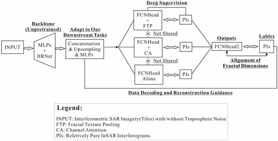
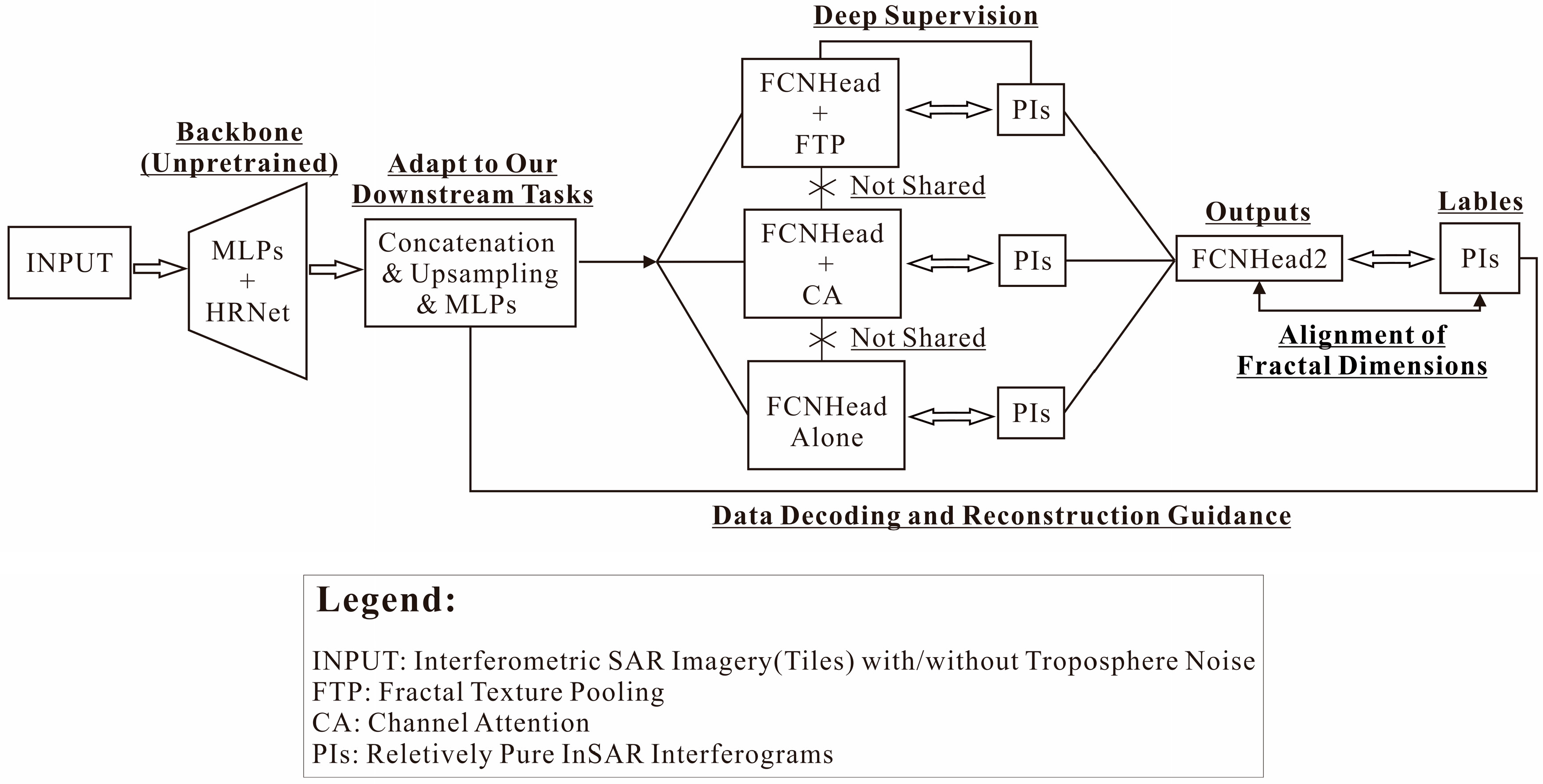
As given in Figure 1, our architecture (termed FANet) is based on HRNet vs. PSPNet (High-Resolution Networks versus Pyramid Scene Parsing Networks), with a customized integration of deep supervision, a fractal pooling module, a fractal dimension-aligning module, a Channel Attention module, and a Domain-Adapting module, each of which is detailed below. Our central objective is to enhance, unleash, and reconstruct noise representations in the latent space while retaining their high-resolution texture.
Figure 1.
The pipeline of our network architecture.
3.2. The Backbone
Our objective is to remove atmospheric noise from InSAR imagery, and the initial step involves introducing a powerful backbone to capture the most essential, diagnostical, informative, and robust deep representations within the raw images. In this study, we choose HRNet-w32 to fulfill this role. One central advantage of HRNet is its ability to maintain high-resolution representations through the parallel multi-branch architecture [12]. It reduces a 512 × 512 × 3 input into a 128 × 128 × 48 (w32) output, with this resolution-preserving capability being critical for our subsequent analyses.
However, the input InSAR data tile is of size 512 × 512 × 1, and two MLP layers are employed to transform it into the HRNet’s input specification, where MLP stands for the Multilayer Perceptron and it is composed of Conv3 × 3 (1 to 9) + Batch Normalization (BN) + ReLU activation followed by Conv3 × 3 (9 to 3 channels) + ReLU. The publicly available pretrained HRNet parameters are unavailable to our study due to the domain and dataset’s mismatch; thus, we must train the backbone from scratch. HRNet is widely used for remote sensing interpretation tasks such as semantic segmentation, change detection, and objects identification; thus, the latent representations must be converted to adapt to our scenario. Herein, we construct a Domain-Adapting gateway, comprising “channel’s concatenation, upsampling from 128 × 128 to 256 × 256, Conv3 × 3 (480 to 640), ReLU, and Conv1 × 1 (640 → 480)” to do the job, enabling gradual knowledge transfer between general feature representations and the APS. While we acknowledge the advantage of Variational Inference (VI) embedded in the latent space, especially its inherent ability to model the uncertainty of APS noise, its drawback is the generation of blurry/smoothed outputs due to its probabilistic nature. Nevertheless, both VI and our customized module can act as the adaptor; yet we opt for the latter due to its smaller size, precision, and lower training cost.
3.3. The Deep Supervision Module
The module is composed of three branches with the unshared learnable parameters, all guided by an FCNHead and supervised by the APS-free SAR images. The FCNHead, used to activate the deep supervision, consists of three convolutional layers: Conv3 × 3 → BN → Dropout → ReLU → Conv3 × 3 → BN → ReLU → Conv1 × 1, where Conv3 × 3 represents the convolutions with a 3 × 3 kernel (stride/padding = 1), and Conv1 × 1 employs a 1 × 1 kernel.
The first branch is equipped with TFP—fractal texture pooling as well. [20] argues that the typical pipeline of “pretrained network → global average pooling (GAP) → fully connected output layer” used in texture recognition has design flaws. GAP, together with other pooling operations, tends to cause a loss of multi-scale, contextual, and spatial information in the feature space, and as given in Equations (1) and (2), he proposed a fractal pooling strategy to preserve these.
where denotes the feature vector (for the -th channel) to be fed into the fully connected layer; represents the Union operation between layers; means convolution operation; I denotes the feature map derived from the Domain-Adapting module; D stands for a differential box counting dimension, and its calculation formula f (•) could be found in [20]; A denotes the result of global average pooling on I. The resulting {Feature} could integrate geometric irregularity and the classification of texture. In the one hand, texture exhibits stronger noise resistance, and that is why we choose to introduce FTP herein; in the other hand, cloud clusters or dense APS noise might have their own textures, and we need a further alignment of the fractal dimension between the predicted and real PIs (pure InSAR) at the top of FANet. The implementation of Equations (1) and (2) in Python 3.1, along with their interface to other convolutional layers, could also be found in [20] and the references therein.
D = f (ReLU(BatchNorm(Conv1 × 1(I))), A = GAP(I)
The second branch is equipped with CA—channel attention. CA is broadly employed to select the channel features discriminative for the current task while suppressing ineffective/redundant ones; and just like the notions of remote sensing’s spectral interpretation, we introduce CA to filter out noise-sensitive channels [27]. However, Dropout must be reduced (let p = 0.01) within the FCNHead paired with CA to prevent interference. The third branch features FCNHead alone, equipped with a dilated convolution layer to enlarge the receptive field without increasing the number of parameters. Branched structures represented by ASPP (Atrous Spatial Pyramid Pooling) are mainly designed to address scale variation in ground objects. The APS noise, however, is a different problem that requires targeted solutions; herein we choose to analogize different scales to the physical properties of noise (e.g., geometrical, spectral, and contextual features), which are then concatenated to form comprehensive features. Unlike ASPP, where scale variation is targeted at the ground objects themselves, features such as the spectrum, geometry, context reflect different facets of the data, which is why deep supervision must be employed.
3.4. The Output and Supervision
We do not intend to develop complex network architectures for task fulfillment; instead, we emphasize the constraints and benefits that mathematical principles can bring. Accordingly, the output module (FCNHead2) is composed of Conv3 × 3 → BN → ReLU → Conv1 × 1, and the supervision (loss function) is organized as expressed in Equation (3):
where MSE represents the mean-square-error term, and SSIM refers to the Structural Similarity Index Measure, assessing image similarity between the predictions (Preds) and the ground truth (PIs) from three core dimensions: luminance, contrast, and structure. Because an SSIM closer to 1 indicates higher the similarity between the predicted and reference images, 1 − SSIM is used here [28]. In practice, all loss terms were normalized to comparable numerical ranges before summation. Their empirical weighting coefficients were set as 1.0 for MSE, 0.8 for (1 − SSIM), 0.05 for Sparsity, and 0.20 for the Fractal term, respectively. These coefficients were selected according to preliminary convergence experiments to avoid the domination of the optimization process by any single loss component.
Loss = MSE(Preds, PIs) + (1 − SSIM(Preds, PIs)) + Sparsity(r, r0) + Fractal(D_p, D_g)
The term Sparsity is a sparsity penalty term, and as given in Equation (4), Sparsity represents a cumulative Kullback–Leibler divergence working on the latent space S, where r = 0.80 denotes the desired sparsity, and denotes the average activation of hidden unit j within S.
Note that the sparsity penalty versus Dropout in the FCNHead is not a conflict but a complement. Dropout is a form of dynamic or stochastic regularization that enhances the model’s generalization capability. Sparsity is a form of structured or deterministic regularization that helps learn more diagnostic feature representations while deactivating the redundancy ones at a fixed proportion r [29]. Atmospheric signals themselves may exhibit sparsity in certain transform domains—the 960 encoder channels cannot all be effective. To our knowledge, APS noise exhibits spatial correlation, low-frequency components, and terrain dependency, partially overlapping with the signal in both the spectral and spatial domains [30]. Sparsity works within the latent space, while dropout occurs at the decoding stage; specifically, we first remove the redundancy and then the noise. The novelty of our model lies in harnessing their combined effects.
As given in Equation (5), the Fractal term is actually an adversarial-based supervised loss [31]. Its objective is to reconstruct the APS-contaminated phase information, more accurately, to generate it under supervision. The term Fractal (•) consists of two components; the first is used to minimize the discrepancy between D_p (fractal dimension of the predicted PIs) and D_g (dimension of the ground truth PIs) using Huber. Huber is known as a robust loss function for regression; for small errors, it behaves like the MSE, providing relatively smooth gradients and efficient convergence, while for large errors, it behaves like the MAE, reducing the impact of outliers and providing robustness. The function g(•) is used to estimate the fractal dimension, which is given in Equation (6) and identical to the one used in FTP.
where is employed as a feature weight for each channel (k), and is the window size that is resizable. Equation (6) is fully differentiable during the backpropagation. Ref. [32] has developed a framework that leverages the multi-fractal spectrum and the Hölder exponent α to align fractal characteristics both globally and locally. This is worth considering; yet our focus in Equation (5) is on the second term—the adversarial loss. To implement it, we need a discriminator to assign the probability (ranging from 0 to 1) that the input (GT or Pred) is real. In this fashion, the first term plays a supervisory role, and the second acts as the generative part. A larger value of the first term (i.e., when the MSE mode is activated) might imply serious APS interference. In our implementation, the switching strategy for λ was performed on a per-batch basis according to the average batch-level MSE. Specifically, λ was set as 0.8 when the batch-averaged MSE exceeded 0.01, indicating relatively severe APS contamination; otherwise, λ decreased to 0.2 to encourage more autonomous residual-pattern learning under mild atmospheric interference. We consider the discriminator as an auxiliary module for the loss function, not as part of the main architecture shown in Figure 1. It works in the following manner: Preds/PIs → U-Net’s first three stacked Conv3 × 3 Blocks (feature extraction) → Flattening → 2 Stacked Linear Blocks (dimension reduction) → Dropout → one Linear Block + Sigmoid and → Probability ([0, 1])—for a fast estimate as suggested by [33].
Fractal(Pred, GT) = Huber(g(Pred), g(GT)) + λE[logD(GT) + log(1 − D(Pred))]
3.5. The Implementation
Our algorithms were implemented using Python 3.10, and the involved libraries included Numpy 2.4, Pytorch 2.12, Scipy 1.17, Sklearn 1.9, Math 3.14, and so on. The input image tile is of size 512 × 512 × 1, and the online augmentation is executed using the random rotation, random cropping, random imaging adjustments (illumination or noise), and tensorization. The training was conducted on a GPU equipped with an NVIDIA RTX 4090 (24 GB VRAM). The batch size was set to 16, and the Adam optimizer with default control parameters (β1 = 0.90, β2 = 0.999, ε = 1 × 10⁻⁸, and a weight decay parameter 1 × 10⁻⁴) was employed with an initial learning rate of 0.001. The number of training epochs was set to 100 with an early-stopping strategy monitored on the validation subset. Specifically, the training process was terminated when the validation loss failed to decrease continuously over 10 successive epochs. The train/validation/test split ratio was 6:2:2. In addition, online augmentation strategies, including random rotation, random cropping, random illumination perturbation, and random noise injection, were employed to alleviate the risk of overfitting under the relatively modest training dataset size.
Also, our model is quasi-lightweight, and it contains only 10.2 M parameters, with FLOPs of 17.79 G when the input tensor is of size 1 × 1 × 512 × 512 and with pretrained parameters embedded. Prior to the calculation of loss or accuracy, histogram matching was applied between the model’s outputs and the labels (PIs) for the suppression of inter-tile color discrepancies and edge artifacts. As an algebraic behavior, this step is excluded from the backpropagation.
Except for visual exhibition, we choose to employ five key image-quality-assessment metrics for comprehensive performance evaluation: MSE (Mean Squared Error); NSE (short for “Nash–Sutcliffe Efficiency”; a comprehensive assessment metric of model prediction efficiency, with a range of (−∞, 1]; and values closer to 1 indicate better model performance); MAE (Mean Absolute Error; average absolute deviation between predicted and true values; and lower values indicate higher accuracy); SSIM (Structural Similarity Index, which evaluates preservation of brightness, contrast, and structural information, with a range of [−1, 1], where values closer to 1.0 indicate higher similarity); and T_Corr (original correlation coefficient between inputs and PIs vs. the coefficient after reconstruction). The four former metrics are included at the suggestion of [9], while the last one is our proposal.
4. Results
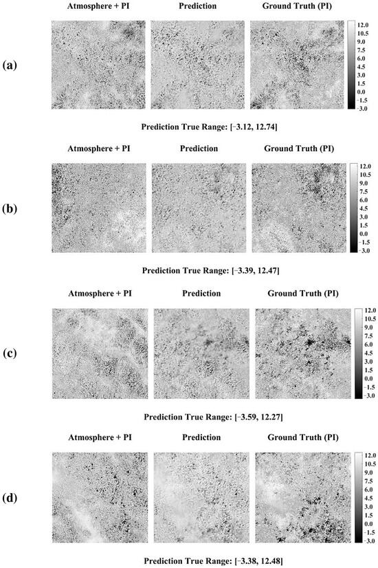
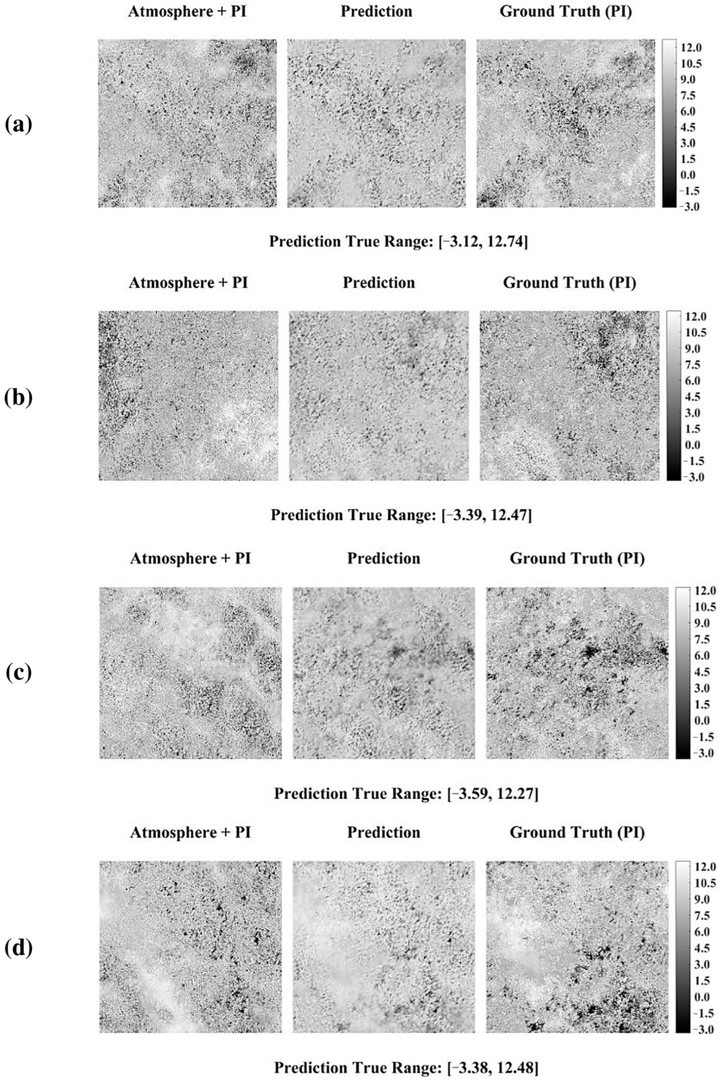
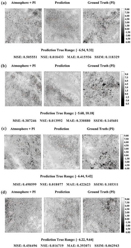
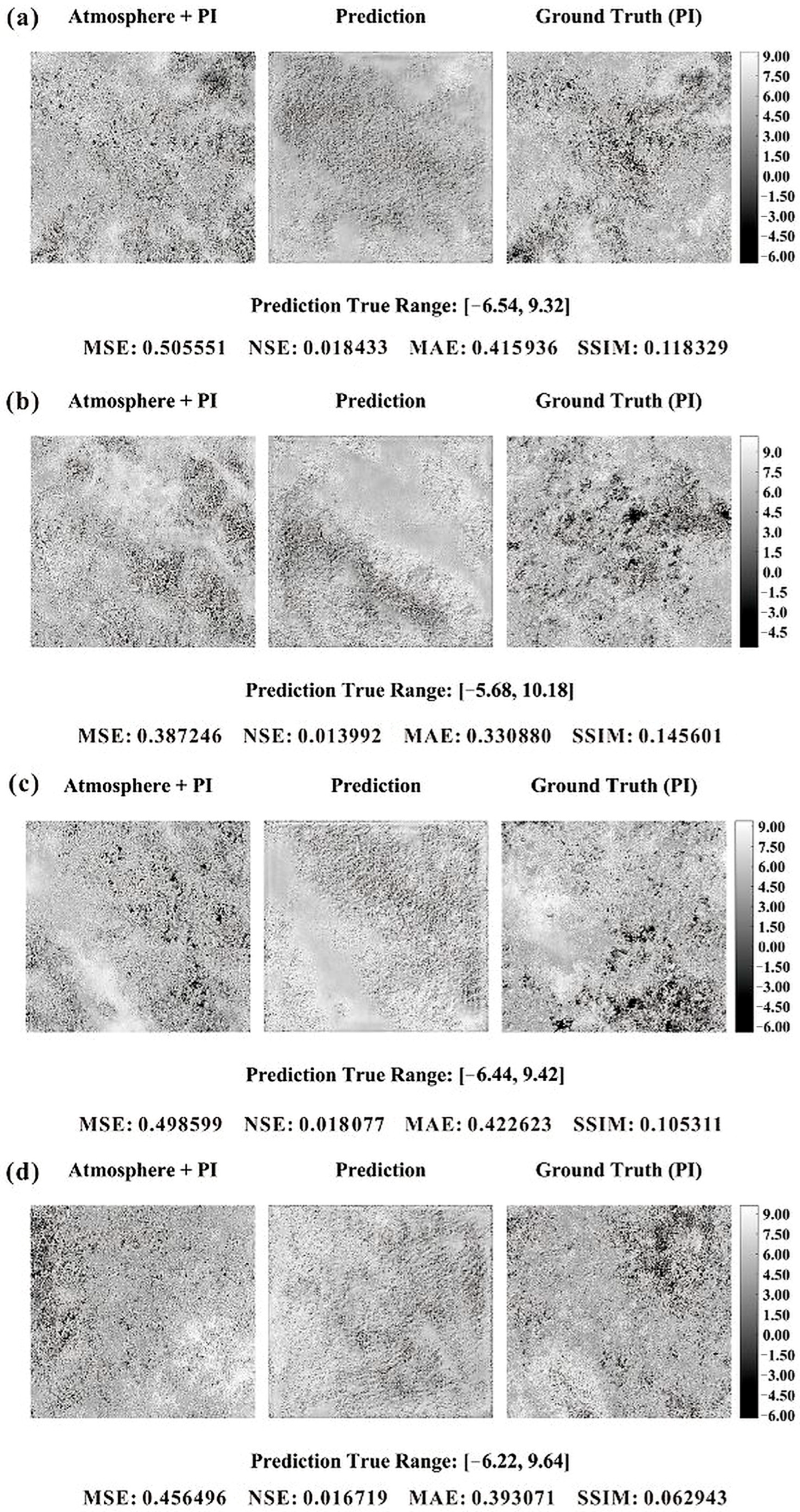
Figure 2 illustrates the resulting noise-free reconstructions using our proposed model, which were selected from the prediction set (1000 tiles) at random. Visually, the obtained images appear free of noise and somewhat similar to the reference PIs; yet they exhibit a coarser granularity than both inputs and outputs. This might be linked to the up-sampling step.
Figure 2.
(a–d) were randomly selected from the prediction set of our mode. Their values were normalized into [0, 1], while its range of true value is given at the bottom of each example.
The data-reconstruction task shown herein has its own characteristics: (1) it is not like the typical denoising calculation, where the noise is learnable with regular patterns (such as white noise); (2) it is, in nature, more like a regression problem (to establish the links between APS and PIs), rather than a reconstruction problem; (3) it requires recovering the underlying topographical phase information by removing APS, yet when atmospheric interference is strong (such as dense rain-bearing clouds), the underlying information is completely missing; (4) there is no perfect regression function or machine learning model capable of retrieving the missing information merely through contextual references. On this occasion, our, or any other, prediction results are bound to partially inherit the APS interference; (5) this has been demonstrated in a closer observation of Figure 2.
Accordingly, the quality metrics specifically calculated for the four representative visualization examples shown in Figure 2 are: MSE = 0.004, NSE = 0.524203, MAE = 0.014211, and SSIM = 0.663017, respectively. These values correspond only to the localized visual samples illustrated in Figure 2, rather than the average performance over the entire prediction set. Since the four representative visualization examples were intentionally selected from relatively interpretable moderate-APS cases, their localized MAE values are naturally smaller than the prediction-set average MAE computed over all testing tiles, including severe APS-contaminated samples.
The comprehensive prediction set mean metrics computed over all 1000 prediction tiles are summarized separately in Table 1. The correction coefficient between the predictions and inputs is 0.5021 (CoC on inputs for short, similarly hereinafter), and CoC on PIs is 0.6705, respectively. It should be noted that these values reflect only the localized performance of these selected visual samples. For the comprehensive evaluation metrics computed over the entire prediction set (1000 tiles), please refer to Table 1 in Section 5. These well meet the industrial requirements; in particular, the correlation balance has started to favor the PIs, which is consistent with our expectations.
Table 1.
Averaged quality metrics of FANet and the compared methods.
5. Discussion
To validate and seek the potential advantages of our proposed model and constraints, comparison and ablation experiments were conducted in this section.
5.1. Compared Methods
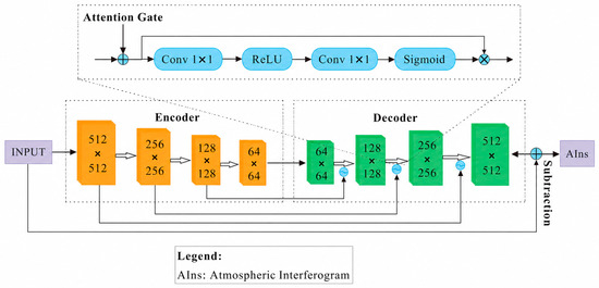
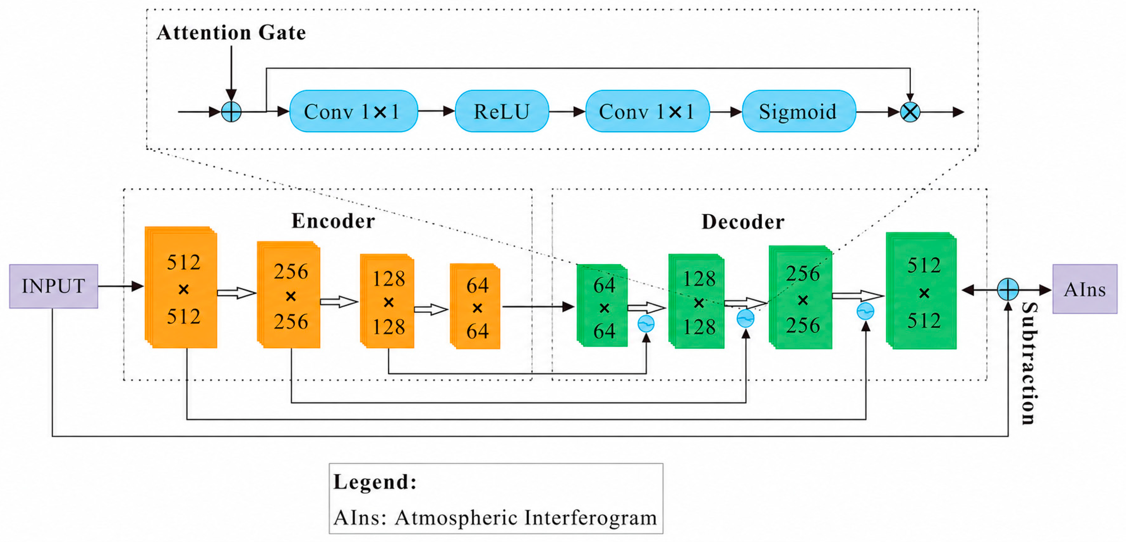
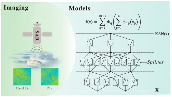
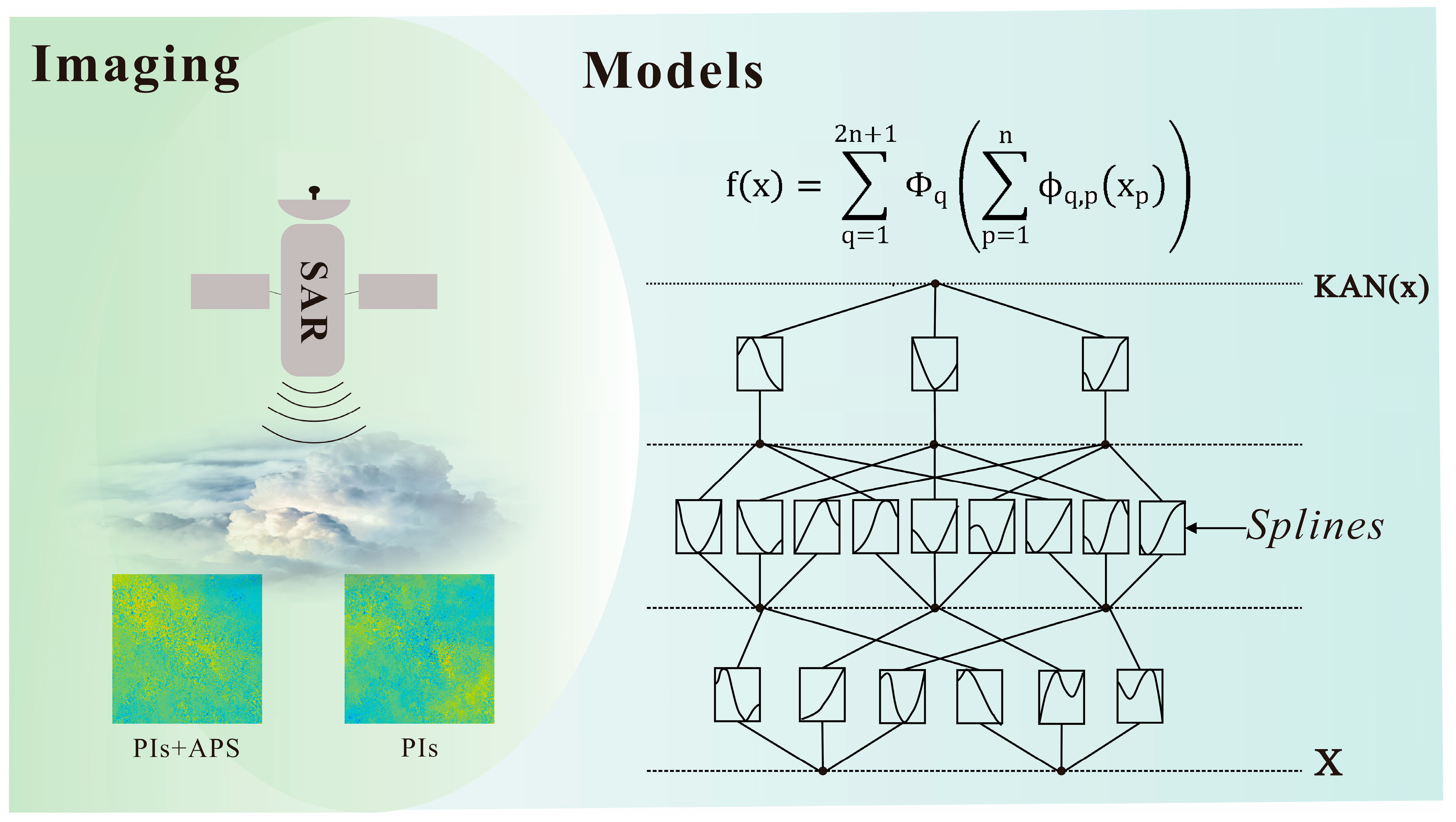
The compared methods to be illustrated include ARU-Net, KAN, and GACOS, which represent deep learning, machine learning under atmospheric physical constraints, and traditional algorithms, respectively [34]. As presented in Figure 3 and Figure 4, their network architectures or working principles are demonstrated separately.
Figure 3.
The network architecture of ARU-Net (modified after [9]). Different colored blocks represent distinct network operations: Attention block, Encoder and Decoder. Blue circles within a wave line in mean activate function. Blue circles within a multiply symbol represent element-wise multiplication.
Figure 4.
The working principle of KAN (modified after [34]). KAN adopts learnable B-spline functions (pq) on the edges connecting the input and the output . This architecture implements a computational paradigm of nonlinear transformation followed by linear combination and SiLU activation. PIs and APS mean pure deformation phase image and atmospheric phase screen, respectively.
As shown in Figure 3, ARU-Net is generally the typical U-Net based, with the exception of an attention gate added to each block of the decoder [9]. Structurally, ARU-Net may perform well in feature refinement yet fails to harness physical constraints. Anyway, refined context-bearing representations are still incapable of filling in the missing and/or severely APS-contaminated phase information of InSAR interferograms. Figure 4 shows the working mechanism of the Kolmogorov–Arnold Network (KAN). Unlike MLPs (Multilayer Perceptrons) that rely on fixed activation functions, such as ReLU, Sigmoid, and the like, attached to nodes and fixed weights for signal transformation, KANs adopt learnable B-spline functions and implement a computational paradigm of “nonlinear transformation first (e.g., in Figure 4, pq represents the B-spline function corresponding to the edge connecting the input and the output ), followed by linear combination ( in Figure 4 + SiLU)”. KANs allow researchers to observe the functional relationships learned by the model intuitively [34], making them a natural tool for rediscovering mathematical and physical laws during our denoising task. However, KANs typically serve as a modular component instead of a complete network architecture. Inasmuch, we choose to integrate them into the latent space of a U-Net. A typical U-Net is composed of nine blocks: four blocks in the encoder, one latent block in the middle, and four decoder blocks; yet we simplified it by using only the first three encoder and decoder blocks, together with the latent block, in order to keep its (termed UNet-KAN) number of parameters consistent with ARU-Net and our FA-Net, and to avoid the risk of computational overhead. GACOS, which is short for the Generic Atmospheric Correction Online Service for InSAR [35], is an open-source online tool dedicated to correcting the APS within InSAR data. GACOS is based on the Iterative Tropospheric Decomposition model, combined with known atmospheric models and multi-source data to achieve accurate separation and/or correction of atmospheric phase delays for InSAR. The GACOS products were downloaded in the zenith-total-delay mode and temporally matched with each Sentinel-1 acquisition according to the corresponding acquisition timestamps.
The compared methods were reimplemented and retrained under unified hardware, dataset, and optimization settings to ensure consistent comparison conditions. Some lightweight simplifications were introduced to maintain comparable parameter scales and computational costs. We acknowledge that such simplifications may reduce the direct comparability with the officially reported performances of the original architecture. The compared methods were re-implemented and retrained under unified hardware, dataset, and optimization settings to ensure consistent comparison conditions. In order to maintain comparable parameter scales and computational costs, lightweight simplifications were introduced for some baseline architectures, including the U-Net + KAN framework. Specifically, the simplified U-Net + KAN adopted only the first three encoder and decoder stages together with one latent block, resulting in an overall parameter scale (~10 M) comparable to ARU-Net and FANet. We acknowledge that these retrained lightweight configurations may differ from the official implementations originally reported in the corresponding studies. Therefore, the present comparisons should primarily be interpreted as evaluations of different architectural philosophies under unified experimental conditions, rather than strict reproductions of the originally published benchmark performances. Figure 5, Figure 6 and Figure 7 and Table 1 exhibit their visual and statistical performance, respectively.
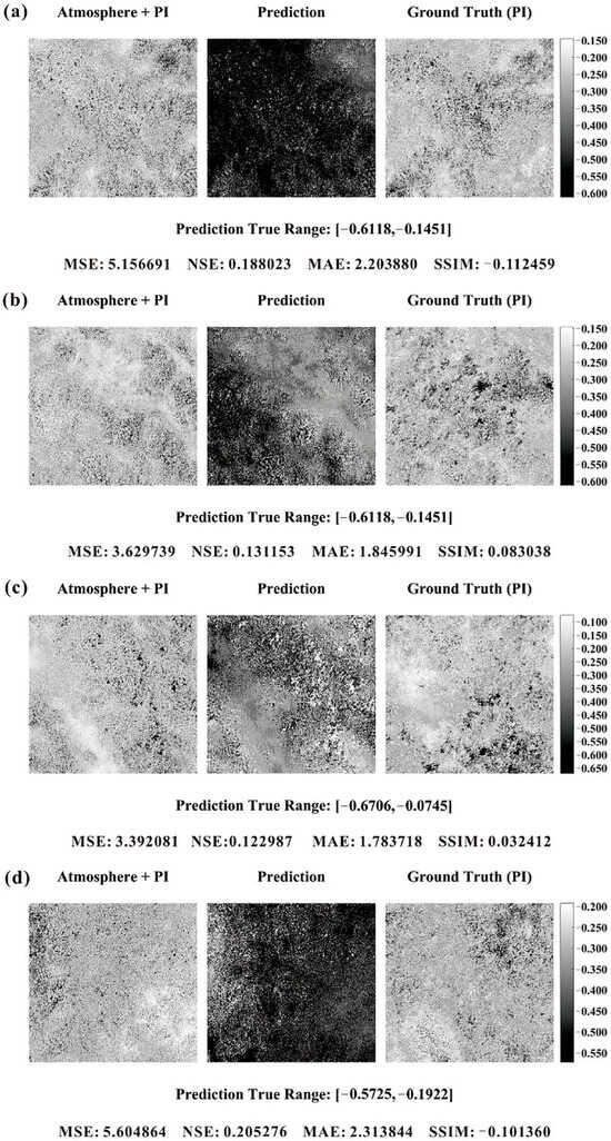
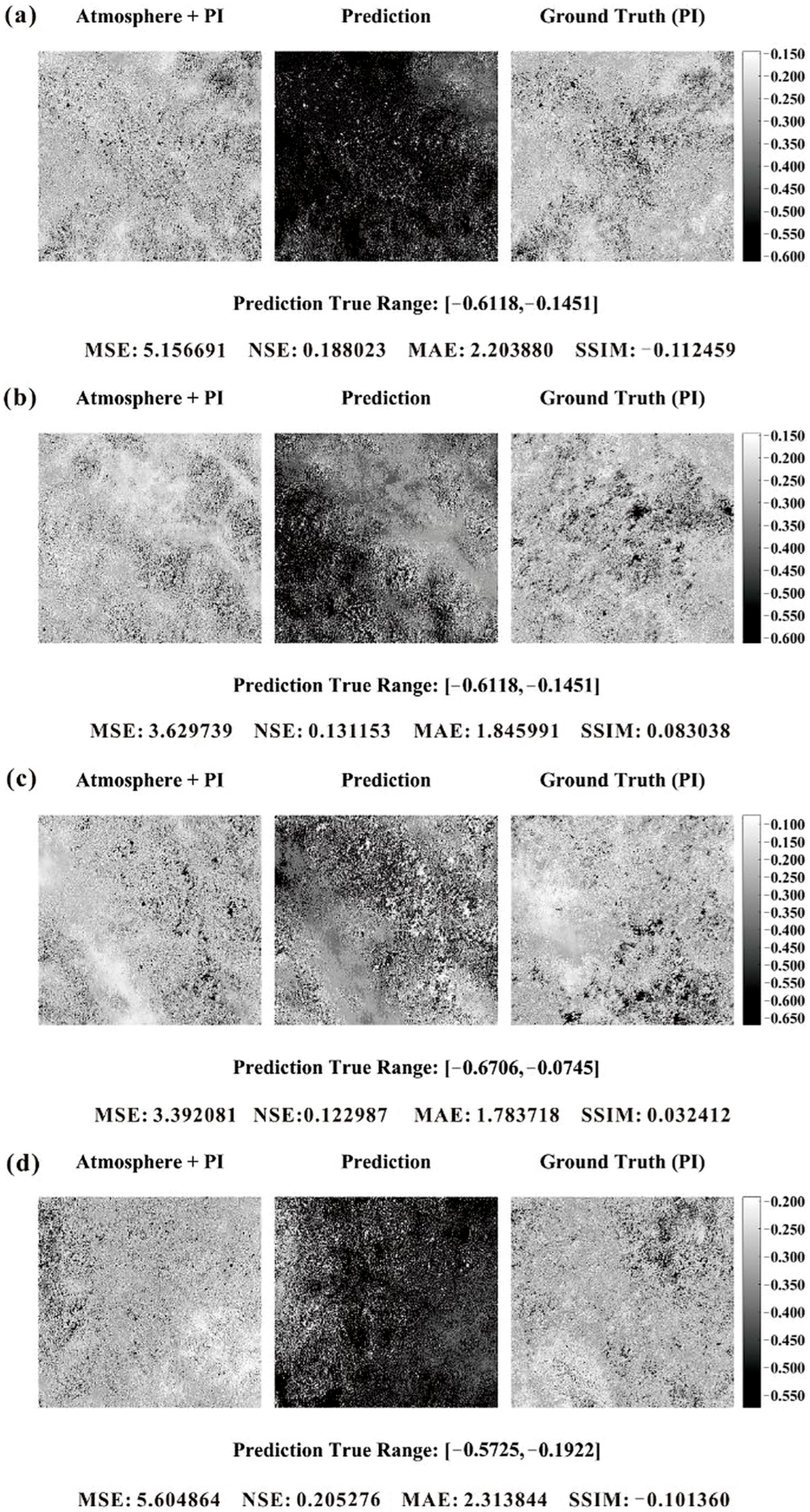
Figure 5.
(a–d) were four selected predictions of ARU-Net, consistent with these in Figure 2.
Figure 6.
(a–d) were four selected predictions of U-Net + KAN, consistent with these in Figure 2.
Figure 7.
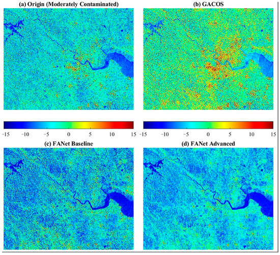
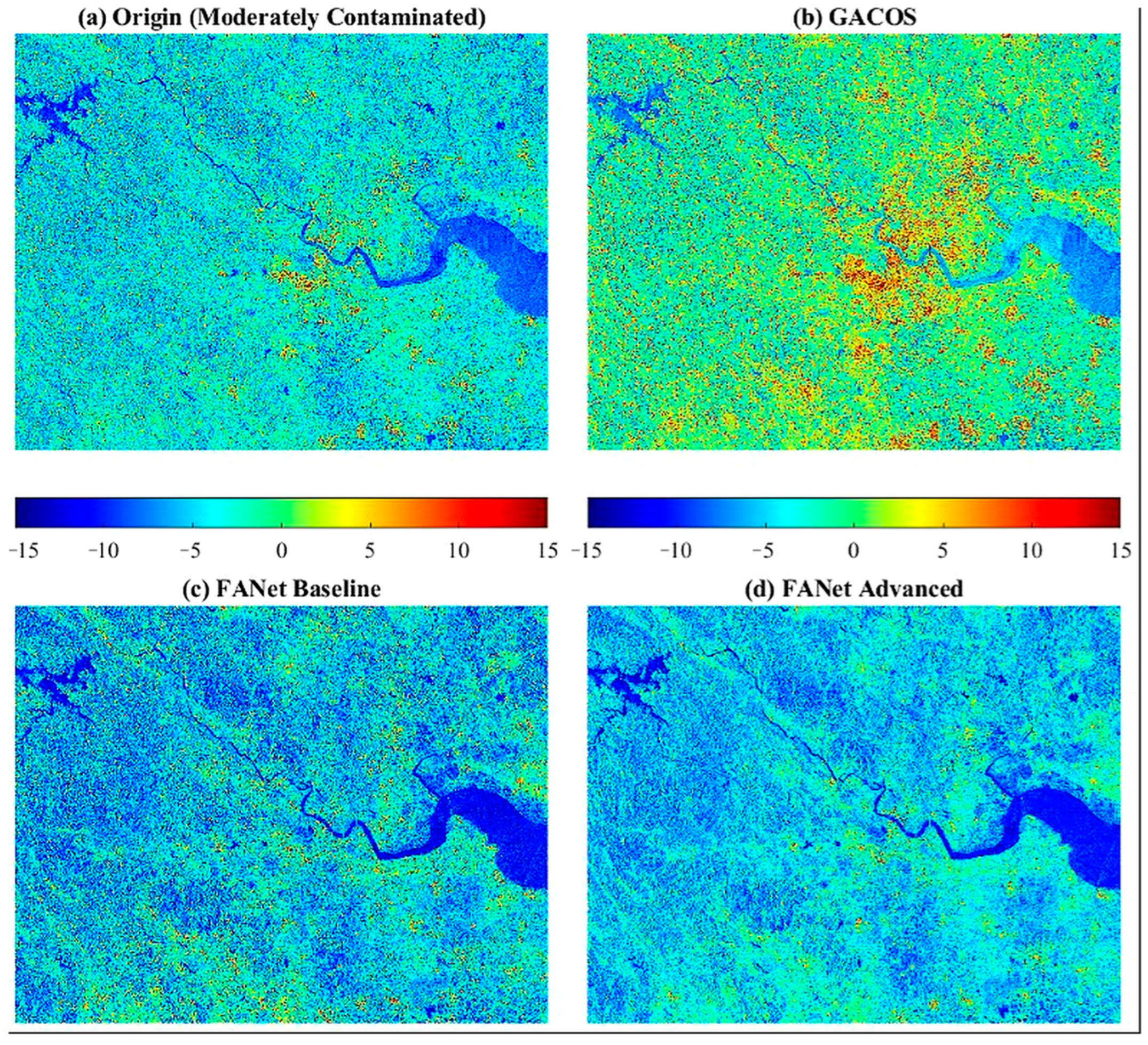
The reconstructions using GACOS over eastern Zhejiang province, China. Note: (a) was collected in June 2024 with moderately contamination (usually shown as colored dots and stripes).
It can be seen from Figure 5, Figure 6 and Figure 7 that the predictions derived from ARU-Net and U-Net + KAN seem more like the inputs themselves, rather than the PIs, despite their seemingly finer granularity. Clearly, this similarity is not an inheritance-based inversion, but simply inheritance itself, and the evidence is that the prediction set average CoC on inputs (0.4–0.7 or so) is 1.5 to 3.0 times larger than the CoC on PIs (for both KAN and ARU-Net). As implied by the MSE, NSE, MAE, and SSIM values labeled at the bottom of each figure, together with the average metrics computed over the prediction set as given in Table 1, the compared methods exhibit even worser APS-denoising performance than ours, despite the rationality of their design philosophies. These findings might highlight three aspects: (1) the compared methods may partially preserve certain interferometric structures under relatively mild APS contamination; however, their overall quantitative performance remains substantially inferior to FANet, especially under complex atmospheric conditions. The U-Net + KAN model attains an SSIM over 0.5 at times (Table 1); in contrast, the cloud-subsurface information could not be created from scratch via contextual data alone when the APS interference becomes severe; (2) as both the APS and topographic details are stochastic, so it is challenging for AI, no matter if it is a CNN, Transformer, or KAN, to learn the general inversion patterns by mapping stochastic-to-stochastic features; and (3), the reason why our proposed FANet has achieved a marginal improvement lies in its information/content-extrapolating ability following the fractal principle.
Figure 7 shows the outputs of GACOS, and as expected, these still do not violate our observations or notions, given GACOS’s drawbacks [36] in the atmospheric model’s generalization and stability [37], spatiotemporal resolution, etc. Figure 7 covers the entire Eastern Zhejiang region, China, and it is composed of 195 tiles with a size 512 × 512. The original imagery was moderately contaminated—the most common scenario encountered in industrial production—and its GACOS version, built on a fixed atmospheric model seems to have amplified such contamination while also bringing about local purification. Our FANet baseline (without the adversarial-based supervision) and FANet perform the best, at least, visually. As a large-area and representative dataset, Figure 7a is sampled randomly in time, and the CoC between GACOS and 7a is 0.97051, between the baseline and 7a is 0.56241, and between the advanced (full) FANet and 7a is 0.52643. The purification process is clearly observable. The high CoC value between GACOS and the original interferograms mainly reflects that GACOS preserves most large-scale low-frequency spatial structures contained in the inputs. However, a high correlation coefficient does not necessarily imply effective APS suppression, especially when atmospheric contamination itself dominates the low-frequency components. In our experiments, GACOS partially reduced some localized atmospheric artifacts while still retaining substantial large-scale APS-related patterns, thereby leading to the coexistence of localized purification and globally high CoC values. Case studies on slight and heavily contamination are not exhibited herein; the former is unrepresentative, and the latter, be it GACOS, FANet or other models, shows poor performance.
The CoC metric was primarily used for localized structural-correlation analyses between the APS-contaminated interferograms, GACOS products, and reconstructed outputs; therefore, it was discussed separately in the corresponding figure analyses rather than being included as a global prediction-set metric in Table 1 and Table 2. The strongly negative NSE values observed for ARU-Net indicate that the reconstructed outputs partially collapse toward overly smoothed, mean-like spatial distributions under severe APS contamination. Such behavior suggests that the model fails to preserve sufficient interferometric variance and fine-scale phase structures in highly corrupted atmospheric conditions.
Table 2.
The average quality metrics of FANet and the derived ablation models.
We acknowledge that more recent architectures, including transformer-based and diffusion/generative paradigms published after 2022, were not fully benchmarked in the present study. The primary objective herein was to compare FANet against representative CNN-based, physics-assisted, and lightweight learning paradigms under unified experimental conditions. Comprehensive comparisons with large-scale generative or transformer-based frameworks remain an important direction for future work.
5.2. Ablation Experiments
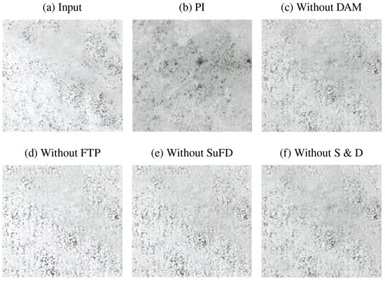
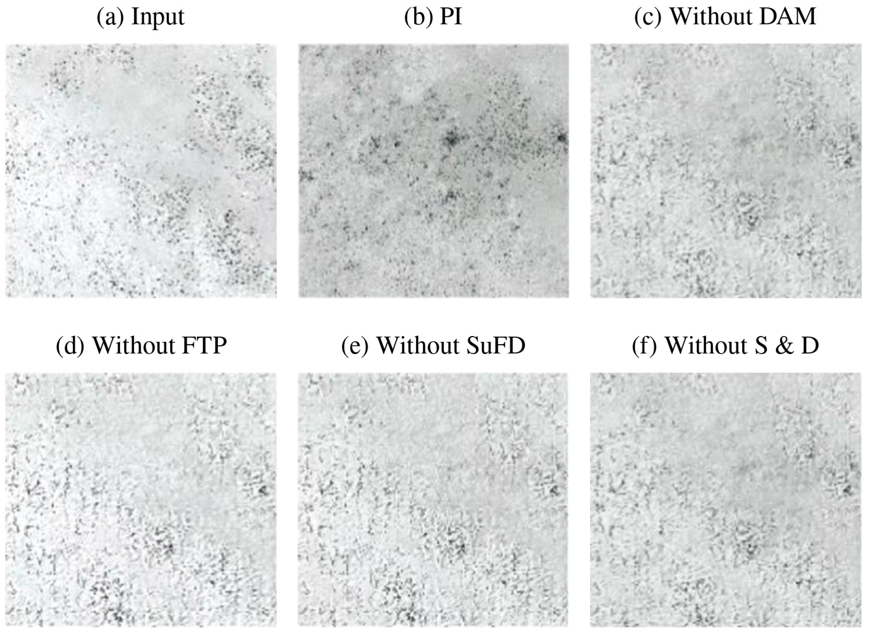
Like what our compared experiments have done, the ablation experiments first require consistent hardware and software conditions (see Section 3.5), environmental configurations, as well as training strategies identical to those of FANet. On this basis, Table 2 gives their quality metrics, and Figure 8 gives their visual performance. Clearly, eliminating the fractal constraints (namely, FTP and fractal dimension-based supervision) severely hurts the model’s predictive capability, followed by the Sparsity and Dropout, while the Domain-Adapting module might have a moderate influence and could be replaced by Variational Inference. Accordingly, their CoC on inputs versus CoC on PIs exhibits analogous traits—a deeper integration of fractal constraints into modeling shifts the correlation balance more toward the PIs, with Sparsity and Dropout further enhancing this trend. The specific MSE, NSE, MAE, SSIM, CoC on inputs, and CoC on PIs of FANet without DAM, FTP, SuFA, and S and D, as well as detailed quantitative comparisons of the ablation experiments, are summarized in Table 2. Overall, removing the fractal-related modules (especially FTP and fractal-dimension supervision) significantly degrades the predictive performance and shifts the correlation balance away from the reference PIs.
Figure 8.
Reconstructions derived from the ablation experiments. The selected example is consistent with the second row of Figure 2.
Although some quantitative metrics between the “Without FTP” configuration and the “U-Net + KAN” baseline appear numerically close, the two frameworks remain fundamentally different in terms of architecture, supervision strategy, and feature representation mechanisms. These figures appear even worse than those of the compared baselines and the average figures in Table 2 over the prediction set, indicating that (1) every module embedded within our proposed model is indispensable, and (2) conventional models or an incomplete FANet remain effective when the APS interference is weak (e.g., (d) in Figure 8). For instance, a peak CoC on PIs of 0.9734 was observed for FANet without FTP in the prediction set.
In mathematics, fractal interpolation works best for recovering missing information from the context, and that is why we use HRNet as our backbone to preserve more contextual details. A dual-guarantee mechanism was proposed herein: in AI, the best way to recover missing information is through “generation”, and we incorporated the Adversarial Loss in the FA-Net. However, our “generation” requires the outputs to align with the PIs not only in terms of statistical distribution but also in content consistency, and we incorporated the dual-fractal constraint (FTP + SuFA) into FA-Net. The contextual clues take a subordinated role.
All average metrics reported in Table 1 and Table 2 correspond to prediction-set means computed over the complete test dataset, while the values presented in Figure 2 correspond only to a few localized visualization examples. Preliminary sensitivity experiments indicate that the proposed framework remains relatively stable when moderate perturbations are introduced into the weighting coefficients, while excessively large fractal-term weights tend to over-smooth the reconstructed phase textures.
5.3. Limitation Analysis and Future Improvements
Although the proposed FANet demonstrates a satisfactory APS suppression capability under moderate atmospheric contamination, the prediction results still exhibit residual coarse-grained interference patterns under severe APS conditions, as already observed in Figure 2. To quantitatively evaluate this limitation, we further conducted a stratified analysis based on APS severity and spatial texture statistics.
First, the prediction set was divided into three categories according to the average coherence coefficient and APS variance, namely weak APS interference, moderate APS interference, and strong APS interference. Table 3 summarizes the corresponding SSIM, MAE, and NSE values under different APS severities. The results indicate that FANet maintains a relatively stable performance under weak-to-moderate APS contamination, while the prediction accuracy decreases significantly when the coherence becomes extremely low or when dense atmospheric disturbances dominate the interferograms. This observation is consistent with our previous conclusion that heavily contaminated APS regions may partially destroy the underlying phase information, making perfect reconstruction theoretically difficult.
Table 3.
Stratified evaluation under different APS severities.
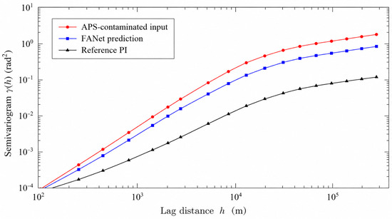
Secondly, to quantitatively characterize the “coarser granularity” phenomenon observed in the FANet predictions, we conducted semi-variogram and frequency-domain analyses over the inputs, predictions, and reference PIs. Figure 9 shows the average semi-variogram curves of the three datasets. Compared with the raw APS-contaminated inputs and the reference PIs, the FANet outputs exhibit enlarged variogram ranges and suppressed nugget effects, indicating that high-frequency atmospheric fluctuations are effectively attenuated, while smoother low-frequency residual structures remain partially preserved. Such behavior explains why the predictions visually appear cleaner but slightly coarser than the ground-truth PIs.
Figure 9.
Semi-variogram comparison among APS-contaminated inputs, FANet predictions, and reference PIs. The FANet outputs exhibit enlarged variogram ranges and reduced nugget effects compared with the raw inputs, indicating suppression of high-frequency APS fluctuations together with partial preservation of coarse-grained residual structures.
Future work may integrate GACOS and FANet in a serial residual-learning configuration. In this strategy, GACOS would first remove the large-scale, physically modeled tropospheric delays, while FANet would subsequently learn the residual APS patterns and reconstruct the remaining interferometric structures. Such a hybrid framework may help reduce the coarse-grained residual artifacts observed in the present study, especially under severe atmospheric contamination conditions.
The above findings suggest that FANet behaves more like an APS-suppression framework than a complete atmospheric inversion model. When the atmospheric contamination becomes extremely severe, the underlying interferometric structures may already be partially destroyed within the inputs themselves, thereby limiting the recoverability of fine-scale phase details through contextual learning alone.
The variogram analysis further supports the necessity of introducing statistical-geometric constraints into APS-suppression tasks. Although the proposed fractal-aware strategy effectively reduces the high-frequency atmospheric interference, the remaining low-frequency residual structures indicate that statistical fractal constraints alone may still be insufficient for completely reconstructing missing phase information under complex atmospheric conditions.
6. Conclusions
This article presents a comprehensive geometry-aware deep learning framework using fractal properties for atmospheric noise removal in InSAR interferograms. The model is termed FANet, which integrates fractal texture pooling, a dropout-sparsity autoencoder, channel attention, a domain-adapting module, user-defined deep supervision, HRNet, and a hybrid loss function. Our findings based on the comparative and ablation experiments indicate that: (1) the compared methods perform reasonably well under moderate APS interference; yet, the under-cloud content cannot be created from scratch via the contextual information alone when the APS interference is severe; (2) both the APS and topographic details are stochastic; hence, it is challenging for AI, no matter if it is a CNN, GACOS or KAN, to learn general inversion patterns by mapping stochastic-to-stochastic features; (3) our FANet achieved a marginal improvement owing to its content-extrapolating ability following the fractal constraints; (4) the Sparsity and Dropout modules could facilitate shifting the correlation balance more toward the PIs; (5) despite partial improvements in inversion, our proposed model still fails to fully eliminate patterns of APS interference, which remain embedded within its predictions with a coarser granularity. Although FANet demonstrates an improved APS suppression capability compared with the representative baselines, the current framework should still be regarded as an APS-suppression and reconstruction framework rather than a complete atmospheric inversion solution, particularly under severe APS contamination conditions. Further work, such as testing the combined use of GACOS and FANet or its variants, must be done to solve these issues.
Author Contributions
P.T.: Funding acquisition, Conceptualization, Methodology, Data curation (SAR data processing and training sample generation), Writing—original draft. B.Z.: Software (implementation and testing of the core algorithms), Validation, Writing—original draft (algorithm section); X.S.: partner of funding providers, Methodology; Y.L.: testing of algorithms, drawing figures. All authors have read and agreed to the published version of the manuscript.
Funding
This study is financially supported by a scientific research project titled “Research of Deep learning technique for atmospheric noise removal in time series InSAR” sponsored by State Key Laboratory of Earthquake Dynamics (Project No. LED2023B01).
Data Availability Statement
All Sentinel-1 SAR data are available at the Alaska Satellite Facility Search Portal (ASFSP): https://search.asf.alaska.edu/.
Acknowledgments
Constructive comments were provided by several anonymous reviewers, and the authors would like to thank them here.
Conflicts of Interest
The authors declare no conflicts of interest.
References
- Meng, L.; Yan, C.; Lv, S.; Sun, H.; Xue, S.; Li, Q.; Zhou, L.; Edwing, D.; Edwing, K.; Geng, X.; et al. Synthetic aperture radar for geosciences. Rev. Geophys. 2024, 62, e2023RG000821. [Google Scholar] [CrossRef] [Scilit]
- Guarnieri, A.M.; Leanza, A.; Recchia, A.; Tebaldini, S.; Venuti, G. Atmospheric phase screen in GEO-SAR: Estimation and compensation. IEEE Trans. Geosci. Remote Sens. 2017, 56, 1668–1679. [Google Scholar] [CrossRef] [Scilit]
- Schüler, T. The TropGrid2 standard tropospheric correction model. GPS Solut. 2014, 18, 123–131. [Google Scholar] [CrossRef] [Scilit]
- Meroni, A.N.; Montrasio, M.; Venuti, G.; Barindelli, S.; Mascitelli, A.; Manzoni, M.; Monti-Guarnieri, A.V.; Gatti, A.; Lagasio, M.; Parodi, A.; et al. On the definition of the strategy to obtain absolute InSAR Zenith Total Delay maps for meteorological applications. Front. Earth Sci. 2020, 8, 359. [Google Scholar] [CrossRef] [Scilit]
- Maciejewska, A. Use of Tropospheric Delay in GNSS-Based Climate Monitoring—A Review. Remote Sens. 2025, 17, 1501. [Google Scholar] [CrossRef] [Scilit]
- Liao, M.; Balz, T.; Rocca, F.; Li, D. Paradigm changes in Surface-Motion estimation from SAR: Lessons from 16 years of Sino-European cooperation in the dragon program. IEEE Geosci. Remote Sens. Mag. 2020, 8, 8–21. [Google Scholar] [CrossRef] [Scilit]
- Guo, S.; Zuo, X.; Zhang, J.; Yang, X.; Huang, C.; Yue, X. Mountain Landslide Monitoring Using a DS-InSAR Method Incorporating a Spatio-Temporal Atmospheric Phase Screen Correction Model. Remote Sens. 2024, 16, 4228. [Google Scholar] [CrossRef] [Scilit]
- Zhang, X.; Li, T.; Zhang, X.; Zhou, X.; Lu, J.; Zhang, X. LT-1 SAR Satellite Constellation for Permafrost Deformation Monitoring Along the Tibetan Plateau Engineering Corridor. Int. Arch. Photogramm. Remote Sens. Spat. Inf. Sci. 2024, 48, 875–880. [Google Scholar] [CrossRef] [Scilit]
- Chen, Y.; Bruzzone, L.; Jiang, L.; Sun, Q. ARU-net: Reduction of atmospheric phase screen in SAR interferometry using attention-based deep residual U-net. IEEE Trans. Geosci. Remote Sens. 2020, 59, 5780–5793. [Google Scholar] [CrossRef] [Scilit]
- Giusti, E.; Gelli, S.; Martorella, M. A parametric-model-based approach for atmospheric phase screen removal in ground-based interferometric SAR. IEEE J. Sel. Top. Appl. Earth Obs. Remote Sens. 2021, 15, 889–900. [Google Scholar] [CrossRef] [Scilit]
- Murdaca, G.; Rucci, A.; Prati, C. Deep learning for InSAR phase filtering: An optimized framework for phase unwrapping. Remote Sens. 2022, 14, 4956. [Google Scholar] [CrossRef] [Scilit]
- Wang, J.; Li, C.; Li, L.; Huang, Z.; Wang, C.; Zhang, H. Atmospheric Phase Screen Reconstruction in SAR Interferometry Using ACGAN Network. In Proceedings of the IEEE International Geoscience and Remote Sensing Symposium (IGARSS), Pasadena, CA, USA, 16–21 July 2023; pp. 8230–8233. [Google Scholar]
- Shao, Y.; Jiang, L.; Yang, B.; Zhou, Z.; Zhang, S.; Chen, Y. A Sparse Convolution Method to Reduce the Atmospheric Phase Screen of SAR Interferometry in the Coastal Region. IEEE Trans. Geosci. Remote Sens. 2024, 62, 1–17. [Google Scholar] [CrossRef] [Scilit]
- Aghababaei, H.; Ferraioli, G.; Vitale, S.; Stein, A. A Deep Learning Solution for Phase Screen Estimation in SAR Tomography. IEEE Geosci. Remote Sens. Lett. 2025, 22, 1–5. [Google Scholar]
- Zhao, Z.; Ding, X.; Prakash, B.A. PINNsFormer: A Transformer-Based Framework For Physics-Informed Neural Networks. In Proceedings of the 12th International Conference on Learning Representations (ICLR), Vienna, Austria, 7–11 May 2024. [Google Scholar]
- Jung, J.; Kim, D.; Park, S. Correction of Atmospheric Phase Screen in Time Series InSAR Using WRF Model for Monitoring Volcanic Activities. IEEE Trans. Geosci. Remote Sens. 2014, 52, 2684–2695. [Google Scholar] [CrossRef] [Scilit]
- Li, J.; Yang, S.; Guo, L. Electromagnetic waves propagation in hypersonic turbulence using fractal phase screen method. J. Electromagn. Waves Appl. 2017, 31, 250–262. [Google Scholar]
- Larsson, G.; Maire, M.; Shakhnarovich, G. Fractalnet: Ultra-deep neural networks without residuals. arXiv 2016, arXiv:1605.07648. [Google Scholar]
- Li, T.; Sun, Q.; Fan, L.; He, K. Fractal generative models. arXiv 2025, arXiv:2502.17437. [Google Scholar]
- Florindo, J.B. Fractal pooling: A new strategy for texture recognition using convolutional neural networks. Expert Syst. Appl. 2024, 243, 122978. [Google Scholar] [CrossRef] [Scilit]
- Zhang, C.; Zuo, R.; Xiong, Y.; Zhao, X.; Zhao, K. A geologically-constrained deep learning algorithm for recognizing geochemical anomalies. Comput. Geosci. 2022, 162, 105100. [Google Scholar] [CrossRef] [Scilit]
- Wang, Z.; Tao, P.; Chen, L. Brain-inspired chaotic spiking backpropagation. Natl. Sci. Rev. 2024, 11, nwae037. [Google Scholar] [CrossRef] [Scilit]
- Myint, S.W. Fractal approaches in texture analysis and classification of remotely sensed data: Comparisons with spatial autocorrelation techniques and simple descriptive statistics. Int. J. Remote Sens. 2003, 24, 1925–1947. [Google Scholar] [CrossRef] [Scilit]
- Drzewiecki, W.; Wawrzaszek, A.; Krupiński, M.; Aleksandrowicz, S.; Bernat, K. Applicability of multifractal features as global characteristics of WorldView-2 panchromatic satellite images. Eur. J. Remote Sens. 2016, 49, 809–834. [Google Scholar] [CrossRef] [Scilit]
- Wang, J.; Sun, K.; Cheng, T.; Jiang, B.; Deng, C.; Zhao, Y.; Liu, D.; Mu, Y.; Tan, M.; Wang, X.; et al. Deep High-Resolution Representation Learning for Visual Recognition. IEEE Trans. Pattern Anal. Mach. Intell. 2020, 43, 3349–3364. [Google Scholar] [CrossRef] [Scilit] [PubMed]
- Alparone, L.; Arienzo, A.; Lombardini, F. Improved Coherent Processing of Synthetic Aperture Radar Data through Speckle Whitening of Single-Look Complex Images. Remote Sens. 2024, 16, 2955. [Google Scholar] [CrossRef] [Scilit]
- Park, W.; Choi, Y.; Mekala, M.S.; Choi, G.S.; Yoo, K.Y.; Jung, H.Y. A Latency-Efficient Integration of Channel Attention for ConvNets. Comput. Mater. Contin. 2025, 82, 3965–3981. [Google Scholar] [CrossRef] [Scilit]
- Zhao, H.; Gallo, O.; Frosio, I.; Kautz, J. Loss Functions for Image Restoration with Neural Networks. IEEE Trans. Comput. Imaging 2017, 3, 47–57. [Google Scholar] [CrossRef] [Scilit]
- Sabokrou, M.; Fathy, M.; Hoseini, M. Video anomaly detection and localisation based on the sparsity and reconstruction error of auto-encoder. Electron. Lett. 2016, 52, 1122–1124. [Google Scholar] [CrossRef] [Scilit]
- Bai, M.; Mao, J.; Li, J.; Zhao, H. Simulation Analysis of the Non-Kolmogorov Atmospheric Turbulence Detected by a Mie-Scattering Lidar Based on the Fractal Method. J. Atmos. Ocean. Technol. 2025, 42, 991–1008. [Google Scholar] [CrossRef] [Scilit]
- Curry, G.D. Supervising across generations. In Security Supervision and Management; Butterworth-Heinemann: Oxford, UK, 2015; pp. 241–255. [Google Scholar]
- Aleksandrowicz, S.; Wawrzaszek, A.; Drzewiecki, W.; Krupiński, M. Change Detection Using Global and Local Multifractal Description. IEEE Geosci. Remote Sens. Lett. 2016, 13, 1183–1187. [Google Scholar] [CrossRef] [Scilit]
- Schonfeld, E.; Schiele, B.; Khoreva, A. A U-Net Based Discriminator for Generative Adversarial Networks. In Proceedings of the IEEE/CVF Conference on Computer Vision and Pattern Recognition (CVPR), Seattle, WA, USA, 13–19 June 2020; pp. 8207–8216. [Google Scholar]
- Fakhoury, D.; Speleers, H. On the expressivity of the ExSpliNet KAN model. J. Comput. Appl. Math. 2026, 476, 117053. [Google Scholar] [CrossRef] [Scilit]
- Yu, C.; Li, Z.; Penna, N.T.; Crippa, P. Generic atmospheric correction model for interferometric Synthetic Aperture Radar observations. J. Geophys. Res. Solid Earth 2018, 123, 9202–9222. [Google Scholar] [CrossRef] [Scilit]
- Zhao, L.; Liang, R.; Shi, X.; Dai, K.; Cheng, J.; Cao, J. Detecting and Analyzing the Displacement of a Small-Magnitude Earthquake Cluster in Rong County, China by the GACOS Based InSAR Technology. Remote Sens. 2021, 13, 4137. [Google Scholar] [CrossRef] [Scilit]
- Saini, D.; Kumar, S.; Singh, M.K.; Ali, M. Two view NURBS reconstruction based on GACO model. Complex Intell. Syst. 2021, 7, 2329–2346. [Google Scholar] [CrossRef] [Scilit]

Disclaimer/Publisher’s Note: The statements, opinions and data contained in all publications are solely those of the individual author(s) and contributor(s) and not of MDPI and/or the editor(s). MDPI and/or the editor(s) disclaim responsibility for any injury to people or property resulting from any ideas, methods, instructions or products referred to in the content. |
© 2026 by the authors. Licensee MDPI, Basel, Switzerland. This article is an open access article distributed under the terms and conditions of the Creative Commons Attribution (CC BY) license.