Probabilistic Assessment of Downtime-Related Energy-Service Unavailability, Production Loss and Economic Impact in Continuous Material-Handling Systems

Abstract

Continuous industrial material-handling systems are operationally and energy-intensive technological structures in which downtime affecting one equipment group can reduce the availability of the entire production chain. This study develops a probabilistic framework for assessing downtime impacts when detailed historical event-level downtime records are available, but complete technical and economic equipment parameters are missing. The analysis is based on 6605 downtime records for conveyors, excavators and stackers observed between 2017 and 2025. Historical downtime records were combined with interval-based assumptions for power demand, load factor, handling capacity, electricity price and commodity value, and were propagated through a Monte Carlo simulation with 10,000 iterations. The results revealed a strong concentration of downtime burden. The combination of P–Conveyor–Material Collapse accounted for 32.58% of total downtime, while the top five equipment–fault combinations explained 67.86% of cumulative downtime. At the system level, the median modelled energy-service unavailability reached approximately 4339 MWh, the median production-loss equivalent reached approximately 9279 kt, and the median total economic loss was approximately EUR 209.5 million. The proposed Energy–Economic Impact Index integrated event frequency, downtime severity, energy-service unavailability and economic loss into a single maintenance-prioritisation indicator. The highest-ranked maintenance target was P–Conveyor–Material Collapse, confirming that maintenance priorities should be determined by combined operational, energy-related and economic consequences rather than by event frequency alone. The study demonstrates that historical downtime records can be transformed into a probabilistic decision-support tool for risk-based maintenance planning in industrial systems with incomplete technical and economic data.

1. Introduction

Continuous industrial material-handling systems are essential technological structures in mining and heavy industry. A typical system consists of excavators, long-distance belt conveyors and stackers, which jointly provide high-capacity material transport. Their performance depends on continuous material flow and the coordinated operation of interconnected equipment groups. In such systems, the failure of one equipment group rarely remains an isolated technical event. It can restrict the throughput of the entire technological chain, interrupt production continuity and reduce the productive use of installed energy capacity. Downtime should therefore not be interpreted only as an operational interruption or a maintenance record, but also as a source of energy service unavailability, lost production capacity, and potential economic loss.

This interpretation is particularly important when long-term event-level downtime records are available, but complete technical and economic parameters for the equipment are missing. In practice, operational datasets often include the time of occurrence, downtime duration, equipment category, and failure type, whereas power demand, load factor, handling capacity, operating regime, and internal cost parameters are not recorded in the same system. Under these conditions, deterministic calculation may create a false impression of precision. A probabilistic modelling framework is more appropriate because uncertain technical and economic inputs can be expressed as defensible intervals and propagated through the analytical model.

The methodological basis for this approach is supported by reliability and availability studies that use probabilistic modelling to represent uncertainty in failure, repair, and operational performance. Mirzaei et al. combined fuzzy logic, ANFIS and Monte Carlo simulation to estimate repair time, availability, MTBF, MTTF and MTTR for repairable energy equipment [1]. Crespo Márquez et al. demonstrated the suitability of Monte Carlo simulation for assessing system availability in cogeneration plants under uncertain failure and repair parameters [2]. Zio et al. extended this logic to multi-state systems with operational dependencies and different states of degradation or performance [3]. These studies establish Monte Carlo simulation as a suitable basis for availability-oriented assessment when deterministic input parameters are uncertain.

A second literature stream links downtime to economic consequences. Wolff and Vössing conceptualised downtime cost as a combination of repair cost, lost production output and unused capacity [4]. Edwards et al. applied a comparable perspective to tracked hydraulic excavators in opencast mining, showing that equipment downtime can be associated with productivity losses and economic damage [5]. This economic interpretation is important for the present study because downtime events are evaluated not only as technical interruptions, but also as events that can reduce production capacity and generate monetary loss equivalents.

A third stream concerns the technical behaviour of the analysed groups of equipment. For excavators, Brînaș et al. modelled the drive power of bucket-wheel excavators using specific energy consumption and cutting geometry [6], while Komissarov et al. showed that the energy consumption of single-bucket excavators depends on the operating regime [7]. For stacker–reclaimer systems, Wang et al. analysed dynamic behaviour and failure mechanisms of a bucket-wheel stacker–reclaimer structure [8]. For conveyors, Halepoto and Khaskheli demonstrated that conveyor energy consumption is affected by the belt speed, belt loading and transfer rate [9]. These studies justify using equipment-specific power-demand and capacity intervals rather than a single uniform parameter across all equipment groups.

The need to connect reliability, availability and production capacity is further supported by mining and conveyor studies. Viveros et al. integrated system reliability and productive capacity analysis in a Chilean mining process [10]. Ogunmilua et al. used Weibull modelling to predict belt conveyor failure rates [11], and Norouzi Masir et al. analysed the availability of armoured face conveyor machines in longwall mining [12]. Maintenance-oriented studies further connect downtime reduction with operational efficiency and energy performance. Mohan et al. linked total productive maintenance, machine learning, MTBF and MTTR with zero-downtime objectives [13]. Zou et al. analysed the impact of downtime on energy-efficient manufacturing systems [14] and introduced opportunity windows for energy saving and maintenance in stochastic production systems [15]. Darabnia and Demichela interpreted maintenance as an opportunity for energy savings [16] and later emphasised the importance of maintenance data fields for energy-saving decisions [17]. Bajpai et al. modelled integrated productivity and energy consumption in a serial manufacturing system [18], while Brundage et al. developed sustainable manufacturing indicators that include OEE and energy productivity [19]. Together, these works support the combined assessment of downtime, energy-service consequences and production performance.

Energy-asset and mining-maintenance studies also support the probabilistic interpretation of the impacts of downtime. Eddouh et al. applied Monte Carlo simulation to cost and energy-loss analysis for wind turbine preventive maintenance [20]. Andrawus et al. addressed quantitative maintenance optimisation for wind turbine life-cycle performance [21], and Abdusamad applied Monte Carlo simulation to wind energy reliability analysis [22]. In mining, Peralta et al. linked equipment reliability with energy consumption and greenhouse gas emissions of hauling fleets [23]. Vílchez Torres et al. developed a Monte Carlo-based model for hydraulic shovel maintenance planning [24], and Roy et al. analysed maintainability and reliability in shovel fleets [25]. These studies confirm that maintenance modelling, reliability and energy-related consequences are closely connected in both energy and mining contexts.

The economic and probabilistic line is further developed in studies focused on downtime cost rates, outage losses and advanced simulation. Cheikh et al. showed that the downtime cost rate can influence the performance and robustness of inspection and replacement strategies in Monte Carlo simulations [26]. Suliva and Fenomeno developed a Bayesian network-based approach to determine process downtime costs in industrial plants [27], while Behera et al. proposed a probabilistic approach to assess financial losses from equipment outages caused by voltage sags [28]. Chang et al. used a Monte Carlo simulation to estimate production availability in offshore installations [29]. Crespo Márquez and Iung proposed a structured Monte Carlo approach for assessing system availability and reliability [30]. Cunningham et al. applied delay-time analysis through Monte Carlo simulation [31], and González-Fernández et al. combined Monte Carlo simulation with cross-entropy methods for composite-system reliability evaluation [32]. These studies demonstrate that uncertainty-based modelling is suitable when availability, failure consequences and economic losses must be evaluated under incomplete information.

The reliability of energy infrastructure provides an additional methodological foundation. Bollen developed a method for reliability analysis of industrial distribution systems [33], and Yu and Beck addressed reliability and availability studies for industrial power systems [34]. González-Fernández and Leite da Silva extended reliability assessment to time-dependent systems using sequential cross-entropy Monte Carlo simulation [35]. Nallainathan et al. applied Monte Carlo reliability evaluation to renewable-rich microgrids while accounting for resource and equipment availability [36]. Although these studies are situated in power-system and energy-infrastructure contexts, they underscore the relevance of probabilistic availability assessment for systems where technical uncertainty affects operational performance.

Data-driven maintenance and energy-prediction research further broadens the analytical basis. Bermeo-Ayerbe et al. developed data-driven energy prediction modelling for energy efficiency and maintenance in smart manufacturing systems [37]. Cruz and García highlighted the role of machine learning in predictive maintenance for improving energy efficiency in industrial operations [38]. Ylipää et al. used OEE assessment to identify potential for maintenance improvement [39], while Chehri and Jeon positioned predictive maintenance within the Industrial Internet of Things, where monitoring and analytics support reductions in downtime [40]. Operational planning and stochastic production studies also support the proposed approach. Chen et al. demonstrated that energy-efficient production systems can be improved through schedule-based operations [41]. Binroth and Haboush applied stochastic system modelling to industrial production systems [42], and Brouwers developed probabilistic descriptions of irregular system downtime [43]. Pfaffel et al. reviewed the performance and reliability of wind turbines [44], and Tazi et al. used a hybrid cost–FMEA analysis to assess wind turbine reliability [45]. These studies support a prioritisation index that combines frequency, downtime severity, energy service unavailability, and economic loss.

The broader energy context is relevant, but it is not the central focus of this paper. Previous studies have shown that energy transformation and equipment life-cycle decisions depend on technical, economic, legislative and investment conditions [46,47,48]. In this study, this broader context is used only to position downtime reduction as a practical energy-efficiency improvement in existing industrial systems. Recent fault-diagnosis frameworks also demonstrate the growing role of data-driven methods for identifying and interpreting technical faults in complex equipment systems [49,50]. However, the focus of the present study is not fault diagnosis itself, but the probabilistic assessment of downtime impacts when detailed event-level records are available and complete technical–economic equipment parameters are missing.

The reviewed literature provides strong but fragmented foundations. Some studies focus on reliability and availability, others on downtime costs, equipment-specific technical parameters, maintenance optimisation, energy efficiency or predictive maintenance. However, limited attention has been paid to integrating multi-year, event-level downtime records, uncertain technical inputs, energy-service unavailability, production-loss equivalents, and economic impact into a single probabilistic framework for continuous material-handling systems. This constitutes both a methodological research gap and a practical data gap, because many industrial datasets contain detailed downtime records but lack directly measured equipment power, load factor, production capacity and internal cost values.

This study addresses this gap by developing a Monte Carlo-based framework that extends historical downtime records with interval-based assumptions for equipment power demand, load factor, handling capacity, electricity price and commodity value. The aim is not to reconstruct directly measured electricity consumption during downtime, but to estimate the productive energy-service capacity, production equivalent and economic value that becomes unavailable when critical equipment is out of operation. The framework is applied to downtime events recorded for conveyors, excavators and stackers in a continuous industrial material-handling system. The main literature streams supporting the proposed framework are summarised in

Table 1. Key literature streams supporting the proposed framework.

Literature Stream	Main Contribution to the Present Study	Representative References
Probabilistic reliability and availability modelling	Supports Monte Carlo simulation for repairable systems, system availability and uncertain reliability parameters.	[1,2,3,29,30,31,32,35,36,42,43]
Downtime cost and outage economics	Supports the interpretation of downtime as lost production, unused capacity and probabilistic financial loss.	[4,5,26,27,28]
Equipment-specific behaviour of conveyors, excavators and stackers	Provides technical justification for group-specific power demand, capacity and failure interpretation.	[6,7,8,9,10,11,12,25]
Maintenance, OEE, predictive maintenance and energy efficiency	Supports the link between downtime reduction, maintenance decisions, productive performance and energy efficiency.	[13,14,15,16,17,18,19,20,37,38,39,40,41,44,45]
Broader energy-transition and equipment life-cycle context	Positions downtime reduction as a practical energy-efficiency improvement in existing industrial systems.	[46,47,48]

.

The research questions are formulated as follows:

RQ1: 

Which equipment groups and failure categories contribute most substantially to cumulative downtime in the analysed system?

RQ2: 

How can uncertain technical and economic inputs be incorporated into downtime analysis using Monte Carlo simulation?

RQ3: 

What is the probabilistic energy-service, production and economic impact of downtime under interval-based technical and economic assumptions?

RQ4: 

Which equipment–fault combinations should be prioritised for maintenance when frequency, downtime severity, energy-service unavailability and economic loss are evaluated jointly?

The contribution of this study is methodological, energy-oriented and managerial–economic. Methodologically, it demonstrates how historical downtime records can be used to construct a probabilistic impact model when exact equipment power and capacity values are unavailable. From an energy perspective, it introduces modelled energy-service unavailability as an interpretation of productive capacity lost during downtime. From a managerial–economic perspective, it provides a transparent prioritisation framework for maintenance decisions based on combined downtime frequency, downtime severity, energy-service impact and economic loss.

2. Problem Definition, Data and Simulation Methods

2.1. Analysed System, ISTC Data Source and Research Design

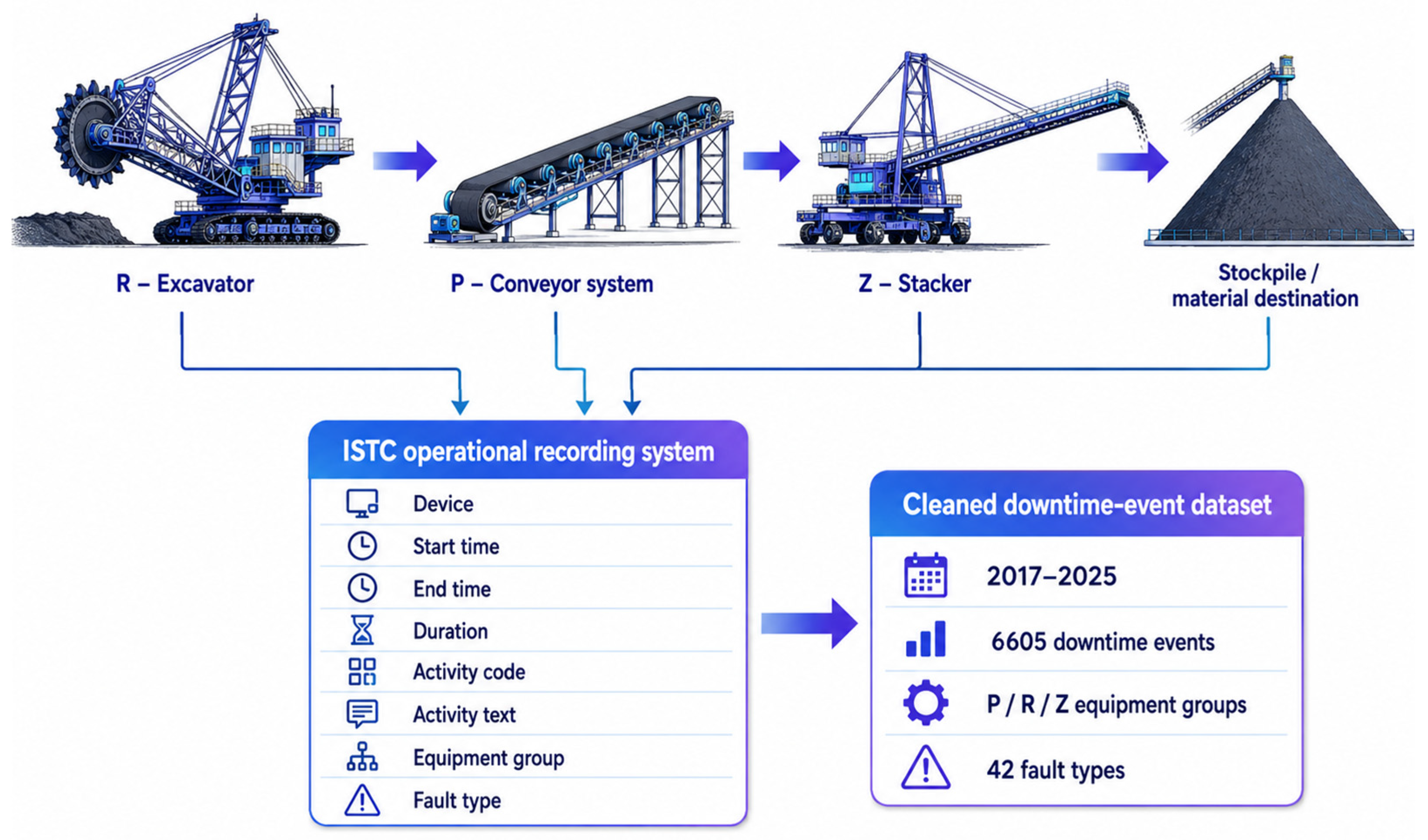
This study investigates downtime in a continuous industrial material-handling system comprising three main equipment groups: conveyors, excavators, and stackers. In the anonymised dataset, these groups are denoted as P–Conveyor, R–Excavator and Z–Stacker. The system’s technological function is based on the continuous movement of bulk material from the excavation point through the conveyor system to the stacking or destination area. Because these machines are operationally interconnected, downtime affecting one equipment group can reduce the availability and productive capacity of the entire material-handling chain.

The operational data were obtained from the internal ISTC system, an information system used to record technological-unit operations. The ISTC system is used to record equipment activities, downtime events, operating states and activity codes during continuous shift operation. Each record includes the affected device, start time, end time, duration, activity code and activity description. The operating day in the recording system follows the plant’s shift logic and is defined as 6:00 to 6:00 of the following day. The system distinguishes between primary activities, which represent the main cause of operational stoppage and are relevant for downtime analysis, and secondary activities, which describe other operational actions that occur during the shift.

The analysed dataset consisted of historical downtime records observed between 2017 and 2025. Each downtime event contained information on the time of occurrence, equipment group, failure or activity characteristic and downtime duration in minutes. The ISTC system provided detailed event-level operational records, but it did not provide directly measured event-level values of equipment power demand, load factor, handling capacity or internal economic loss. These technical and economic parameters were therefore represented by interval-based scenario assumptions and propagated through the Monte Carlo simulation.

The anonymised structure of the analysed material-handling system and the transformation of ISTC records into the cleaned downtime-event dataset are shown in Figure 1.

The analytical workflow consists of three stages. First, the observed downtime structure is examined by equipment group, fault type, equipment–fault combination and time period. Second, uncertain technical and economic inputs are modelled as interval parameters. Third, the observed downtime records are transformed into probabilistic estimates of modelled energy-service unavailability, production-loss equivalent and total economic loss using Monte Carlo simulation. This design follows the general logic of Monte Carlo-based availability and reliability assessment used for repairable energy and industrial systems [1,2,3], production availability modelling [29], structured availability assessment [30] and reliability evaluation under uncertainty [32,35,36].

All data preprocessing, modelling and visualisation were performed in RStudio, using R version 4.5.2. The workflow included data cleaning, date-time parsing, feature engineering, downtime aggregation, Monte Carlo simulation, output aggregation and graphical visualisation. The simulation was repeated 10,000 times, and reproducibility was supported by setting the random seed to 1234 in the R implementation.

2.2. Dataset Preprocessing and Cleaning Rules

The original downtime duration was recorded in minutes and converted to hours. This converted variable served as the primary measure of downtime severity. Calendar variables were derived from the event timestamp, including year, month, quarter, week, day of week and hour of occurrence. Interarrival times between consecutive downtime events were calculated at the overall level and, where analytically relevant, at the equipment-group and fault-type levels. These variables enabled the analysis of downtime concentration, recurrence and temporal clustering. The treatment of downtime as an irregular, stochastic phenomenon is consistent with probabilistic descriptions of system downtime and with stochastic production-system modelling [42,43].

Downtime duration in hours was calculated as follows:

$$D{T}_i={\displaystyle \frac{downtime\_mi{n}_i}{60}}$$

(1)

where $D{T}_i$ is the downtime duration of event $i$ expressed in hours.

The analysis was restricted to equipment groups P, R and Z because these groups correspond to the main continuous material-handling functions investigated in the study. The raw analytical dataset contained 6605 downtime-event records. No missing downtime-duration values were identified. Ten records had zero recorded downtime duration. These records were retained in the descriptive dataset summary because they form part of the original operational record but were excluded from duration-based inferential tests because they do not represent positive equipment unavailability time. Therefore, the Kruskal–Wallis and post hoc Wilcoxon tests were performed on 6595 positive-duration records.

Raw operational fault labels were standardised to professional English fault-type names prior to aggregation. This recoding step was necessary because the original ISTC labels were operational descriptions used in plant recording, whereas the manuscript reports results using consistent technical terminology. The recoded fault types were then used for equipment-level, fault-level and equipment–fault-combination analyses.

2.3. Monte Carlo Input Assumptions

Because directly measured values of equipment power demand, operating load, handling capacity and internal economic loss were not available in the ISTC downtime records, the model used interval-based input assumptions. These assumptions were derived from the cited technical literature, engineering reasoning and externally anchored scenario inputs. The values were not interpreted as exact nameplate measurements or measured operating parameters of the analysed equipment. Instead, they were used as minimum–mode–maximum intervals to propagate technical and economic uncertainty through the Monte Carlo model.

Electricity price assumptions were defined as scenario-based inputs for industrial electricity prices for non-household consumers in the Slovak/Central European context. The interval was anchored to Eurostat electricity price statistics for non-household consumers, where prices are reported in EUR/kWh and differentiated by consumption bands [51]. The electricity price interval was not interpreted as the actual tariff paid by the analysed operator. The commodity-value assumption was formulated as a conservative, low-value bulk-material scenario informed by EIA coal-price data, which show that coal prices differ substantially by coal rank, grade, mining method, and region [52].

Triangular distributions were selected for the most uncertain parameters because they allow the analyst to define a minimum, a most likely value and a maximum value when empirical probability distributions are not available. This choice is consistent with uncertainty-based modelling in availability, reliability and maintenance studies, where input parameters are incomplete or variable [1,2,3,20,24,26,29,30,31,32].

The general form of the triangular distribution was defined as follows:

$$X_j\sim Triangular(X_{min,j},X_{mode,j},X_{max,j})$$

(2)

where $X_j$ is an uncertain technical or economic parameter for equipment group $j$.

The values in

Table 2. Input parameters for the Monte Carlo downtime-impact model.

Parameter	Equipment/ Scenario	Min	Mode	Max	Unit	Use in Model	Basis of Min–Mode–Max Interval	Source Basis
Power demand	P–conveyor	75	315	630	kW	Energy-service loss	Literature-supported conveyor operating range; mode selected as representative medium-load operation	[9]
Power demand	R–excavator	166	700	1410	kW	Energy-service loss	Literature-supported excavator power range; mode selected as representative operating scenario	[6,7]
Power demand	Z–stacker	166	700	1410	kW	Energy-service loss	Stacker–reclaimer technical literature and engineering scenario; mode selected as representative operating scenario	[8]
Load factor	P–conveyor	0.40	0.65	0.90	ratio	Effective power	Engineering scenario reflecting partial, typical and high loading	[9], engineering assumption
Load factor	R–excavator	0.40	0.70	0.95	ratio	Effective power	Engineering scenario reflecting partial, typical and high loading	[6,7], engineering assumption
Load factor	Z–stacker	0.40	0.70	0.95	ratio	Effective power	Engineering scenario reflecting partial, typical and high loading	[8], engineering assumption
Capacity	P–conveyor	60	240	480	t/h	Production-loss equivalent	Literature-supported conveyor transfer-capacity range; mode selected as conservative typical capacity	[9]
Capacity	R–excavator	200	1000	4200	t/h	Production-loss equivalent	Literature-supported excavator capacity interval; mode selected as conservative operating capacity	[5,6,7,25]
Capacity	Z–stacker	200	3000	8000	t/h	Production-loss equivalent	Stacker–reclaimer capacity scenario based on literature and technical reasoning	[8]
Electricity price	Industrial electricity	0.15	0.16	0.23	EUR/ kWh	Energy-service cost equivalent	Eurostat-based non-household industrial electricity-price scenario for Slovak/Central European context	[51]
Commodity value	Low-value bulk material	10	20	40	EUR/t	Production-loss cost	Conservative low-value bulk-material scenario informed by external coal-price information	[52], scenario assumption

are not to be interpreted as exact technical measurements, nameplate parameters, or measured economic values of the analysed equipment. They represent literature-supported and scenario-based interval assumptions used to propagate technical and economic uncertainty through the Monte Carlo model. The resulting outputs should therefore be interpreted as probabilistic decision-support estimates rather than direct metered electricity consumption or accounting losses.

2.4. Monte Carlo Impact Calculation and Simulation Workflow

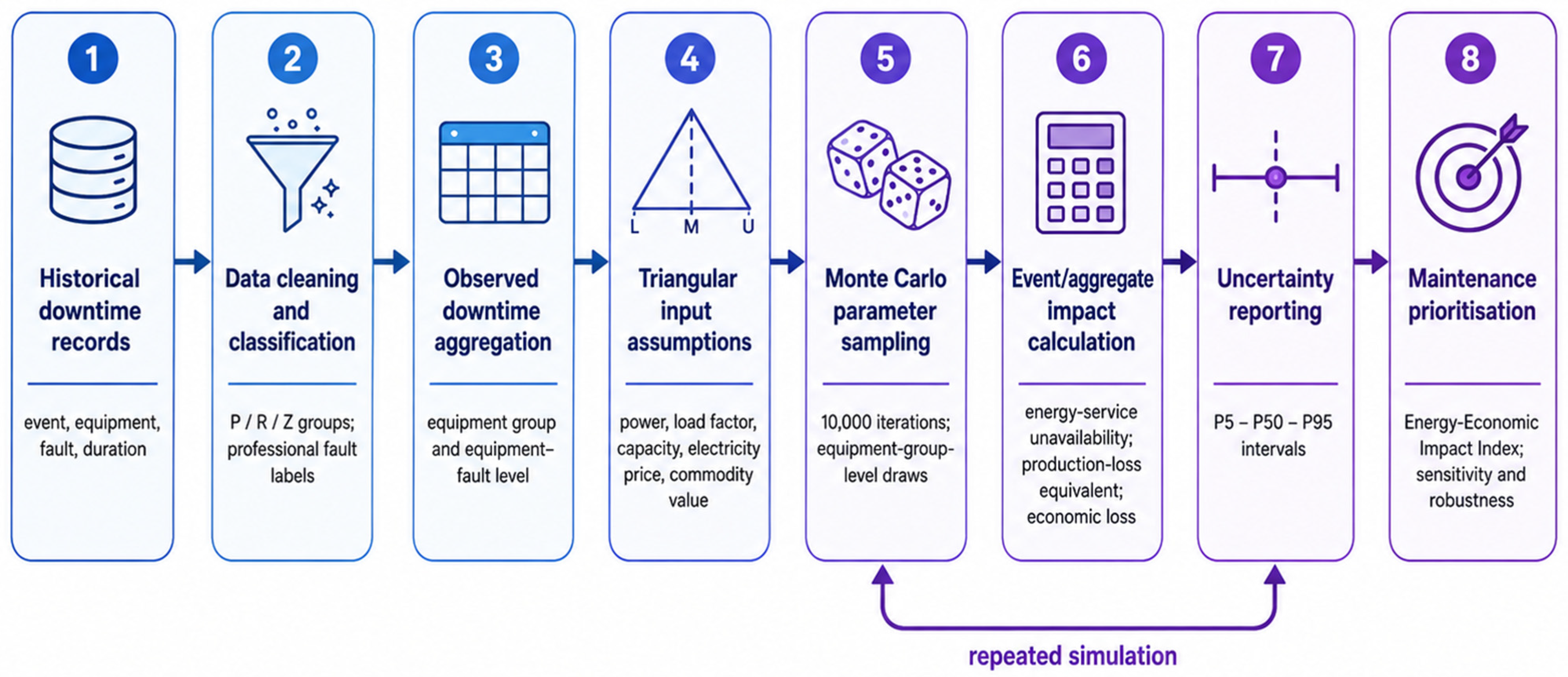
For each Monte Carlo iteration, uncertain technical parameters were sampled at the equipment-group level for P–Conveyor, R–Excavator and Z–Stacker. These sampled values were then combined with the observed downtime records or downtime aggregates corresponding to the respective equipment group or equipment–fault combination. The simulation, therefore, represents uncertainty in group-level technical and economic conditions rather than independent random technical-parameter variation for every individual downtime event. This approach is consistent with the available data structure because the ISTC system records event timing, equipment, and activity information but does not directly provide measured event-level power, load, or capacity values. The complete Monte Carlo downtime-impact simulation workflow is summarised in Figure 2.

The effective power demand of equipment group j was calculated as follows:

$$P_j^{eff}=P_j\times L{F}_j$$

(3)

where $P_j$ is the simulated power demand of equipment group $j$, and $L{F}_j$ is the simulated load factor.

The modelled energy-service unavailability was calculated as follows:

$$E_{loss,i}=D{T}_i\times P_j^{eff}$$

(4)

where $E_{loss,i}$ is the modelled energy-service unavailability of event $i$. This indicator does not represent directly measured electricity consumption during downtime. Rather, it expresses the productive energy-service capacity that was unavailable because the equipment was not operating. This interpretation is consistent with studies that connect downtime, energy efficiency, maintenance and production-system performance [14,15,16,17,18,19,37,38,39,40,41].

The modelled production loss was calculated as follows:

$$Q_{loss,i}=D{T}_i\times C_j$$

(5)

where $Q_{loss,i}$ is the production-loss equivalent of event $i$, and $C_j$ is the simulated production or handling capacity of equipment group $j$. The connection between availability and productive capacity follows the logic of integrated reliability and productive-capacity assessment [10] and downtime-cost modelling based on lost output and unused capacity [4,5].

The energy-service cost equivalent was calculated as follows:

$$Cos{t}_{energy,i}=E_{loss,i}\times Pric{e}_{el}$$

(6)

The production-loss cost was calculated as follows:

$$Cos{t}_{production,i}=Q_{loss,i}\times Valu{e}_t$$

(7)

The total modelled economic loss was calculated as follows:

$$Cos{t}_{total,i}=Cos{t}_{energy,i}+Cos{t}_{production,i}$$

(8)

The total loss indicator is therefore a scenario-based economic estimate, not an accounting measurement. It should be interpreted as a probabilistic approximation of the value-at-risk from downtime, given the assumed technical and economic input intervals. This interpretation is consistent with downtime-cost, outage-loss and cost-impact approaches in industrial and energy systems [4,26,27,28,45], while the monetary input assumptions are anchored in the external electricity and coal price information [51,52].

2.5. Simulation Outputs and Uncertainty Intervals

The Monte Carlo simulation was repeated N_MC = 10,000 times. In each iteration, sampled equipment-group-level technical and economic parameters were combined with the observed downtime structure following the workflow shown in Figure 2. Outputs were then aggregated by equipment group, fault type, equipment–fault combination and time period, depending on the analytical level. The final outputs were summarised using the 5th, 50th and 95th percentiles:

$$Output=\{P5,P50,P95\}$$

(9)

These percentiles represent the lower-bound, median and upper-bound estimates of the simulated output distribution. The main output indicators were cumulative downtime, modelled energy-service unavailability, production-loss equivalent, energy-cost equivalent, production-loss cost and total modelled economic loss. Percentile-based reporting is appropriate because the purpose of the simulation is to quantify uncertainty intervals rather than to provide a single deterministic value.

When availability-equivalent indicators were calculated, downtime was compared with the assumed annual operating-hours scenario:

$$U_g={\displaystyle \frac{\sum _{i\in g}D{T}_i}{H_{op}}},A_g=1-U_g$$

(10)

where $U_g$ is the downtime share of equipment group $g$, $A_g$ is the corresponding availability-equivalent indicator, and $H_{op}$ is the assumed annual operating-hours denominator. Because $H_{op}$ is scenario-dependent, availability-equivalent results should be interpreted as scenario estimates rather than measured availability. This distinction is consistent with the logic of availability benchmarking and Monte Carlo-based reliability assessment [1,2,3,29,30,34,35,36].

2.6. Energy–Economic Impact Index

To support maintenance prioritisation, an Energy–Economic Impact Index was calculated for each equipment–fault combination k. The index combines four dimensions: failure frequency, downtime severity, energy-service unavailability and economic loss. This structure is consistent with studies showing that maintenance priorities should be based not only on failure occurrence but also on downtime costs, production losses, energy impacts, and life-cycle consequences [4,5,13,14,15,16,17,18,19,20,26,27,28,39,44,45].

Each component was normalised before aggregation. A min–max normalisation can be used as follows:

$${\tilde{X}}_k={\displaystyle \frac{X_k-min\left(X\right)}{max\left(X\right)-min\left(X\right)}}$$

(11)

where $X_k$ is the value of a given component for equipment–fault combination $k$, and ${\tilde{X}}_k$ is the normalised value. The Energy–Economic Impact Index was then calculated as follows:

$$EEI{I}_k=w_1{\tilde{F}}_k+w_2{\tilde{D}}_k+w_3{\tilde{E}}_k+w_4{\tilde{C}}_k$$

(12)

where ${\tilde{F}}_k$ is the normalised failure-frequency component, ${\tilde{D}}_k$ is the normalised downtime component, ${\tilde{E}}_k$ is the normalised energy-service component, ${\tilde{C}}_k$ is the normalised economic-loss component, and $w_1$ to $w_4$ are the component weights. In the baseline model, equal weights were used, i.e., $w_1=w_2=w_3=w_4=0.25$. Sensitivity analysis of the weights is recommended because maintenance priorities may change when economic loss or energy-service unavailability is weighted more strongly than event frequency.

The index was used to identify equipment–fault combinations that should be prioritised for maintenance. This is necessary because the most frequent failures are not necessarily the failures with the highest energy-service or economic impact.

2.7. Methodological Limitations

The proposed methodology has several limitations. First, the analysed downtime dataset does not contain directly measured values of equipment power demand, load factor, handling capacity or internal costs. These parameters were therefore represented by interval-based assumptions. Second, the energy-related output is interpreted as modelled energy-service unavailability rather than measured electricity consumption. Third, the economic value of the handled material and the electricity price input were represented using scenario-based intervals, meaning that the results should be interpreted as value-at-risk estimates rather than accounting losses. Fourth, availability-equivalent indicators depend on assumed annual operating-hour scenarios. Fifth, the model represents equipment heterogeneity at the P/R/Z group level and does not fully reconstruct cascading dependencies, buffer effects or redundancy mechanisms across the technological chain.

Despite these limitations, the framework enables historical downtime records to be transformed into probabilistic estimates of the operational, energy-service and economic impact. This provides a transparent basis for maintenance prioritisation in industrial systems where detailed downtime records are available, but complete technical and economic parameterisation is not. The methodology should therefore be interpreted as a transferable modelling procedure rather than as a directly transferable numerical result. Application to other sectors, such as ports, cement plants, steel production logistics or bulk terminals, would require recalibration of equipment-specific power, capacity and economic input intervals.

3. Results

3.1. Basic Structure of the Downtime-Event Dataset

The analysed dataset consisted of 6605 event-level downtime records observed between 2017 and 2025. The total recorded downtime reached 977,890 min, corresponding to 16,298.17 h of equipment unavailability. The analysis focused on three core equipment groups of the continuous material-handling system: P–Conveyor, R–Excavator and Z–Stacker. The dataset also included 42 specific fault types and four broader downtime-character categories.

The mean downtime duration was 148.05 min per event, while the median reached 201 min. The interquartile range of 55–253 min indicates substantial heterogeneity in downtime duration. The recorded minimum and maximum downtime values ranged from 0 to 286 min. Ten zero-duration records were retained in the descriptive dataset summary but excluded from duration-based inferential tests because they do not represent positive equipment-unavailability time.

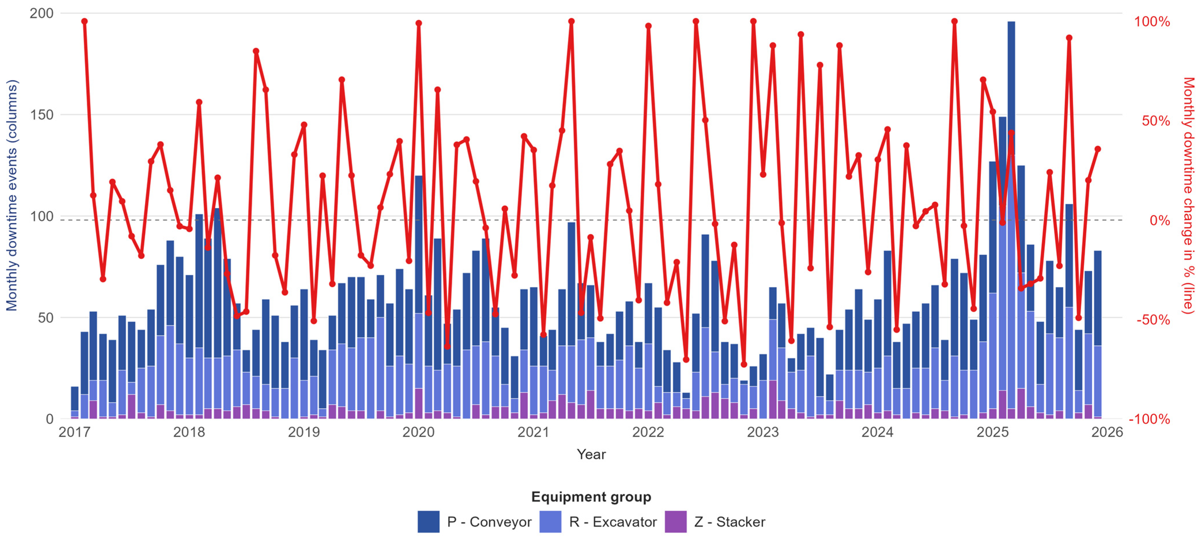
An initial overview of the monthly temporal coverage of downtime records is provided in Figure 3, while the annual temporal development is analysed in detail in Section 3.7.

3.2. Downtime Burden by Equipment Group

The next step of the analysis assessed how downtime events were distributed across the analysed equipment groups. This comparison is necessary because the frequency of recorded events does not necessarily correspond to their cumulative operational burden. Therefore, each equipment group was evaluated not only by event frequency, but also by its share of total downtime, median event duration and burden ratio. The downtime burden indicators by equipment group are summarised in

Table 3. Downtime burden by equipment group.

Equipment Group	Events (n)	Events (%)	Downtime (h)	Downtime (%)	Median Duration (min)	Burden Ratio
P–Conveyor	3395	51.40	13,563.83	83.22	253.0	1.62
R–Excavator	2710	41.03	2219.03	13.62	55.0	0.33
Z–Stacker	500	7.57	515.30	3.16	78.5	0.42

Source: Own processing in RStudio, R version 4.5.2.

.

The results show a highly asymmetric distribution of downtime burden. P–Conveyor accounted for 51.40% of all events but 83.22% of total downtime, corresponding to 13,563.83 h. Its burden ratio reached 1.62, indicating a disproportionate contribution to downtime relative to event frequency. By contrast, R–Excavator accounted for 41.03% of events but only 13.62% of downtime, while Z–Stacker represented 7.57% of events and 3.16% of downtime. These results confirm that conveyors were the dominant source of cumulative downtime.

3.3. Distribution and Severity of Downtime Duration

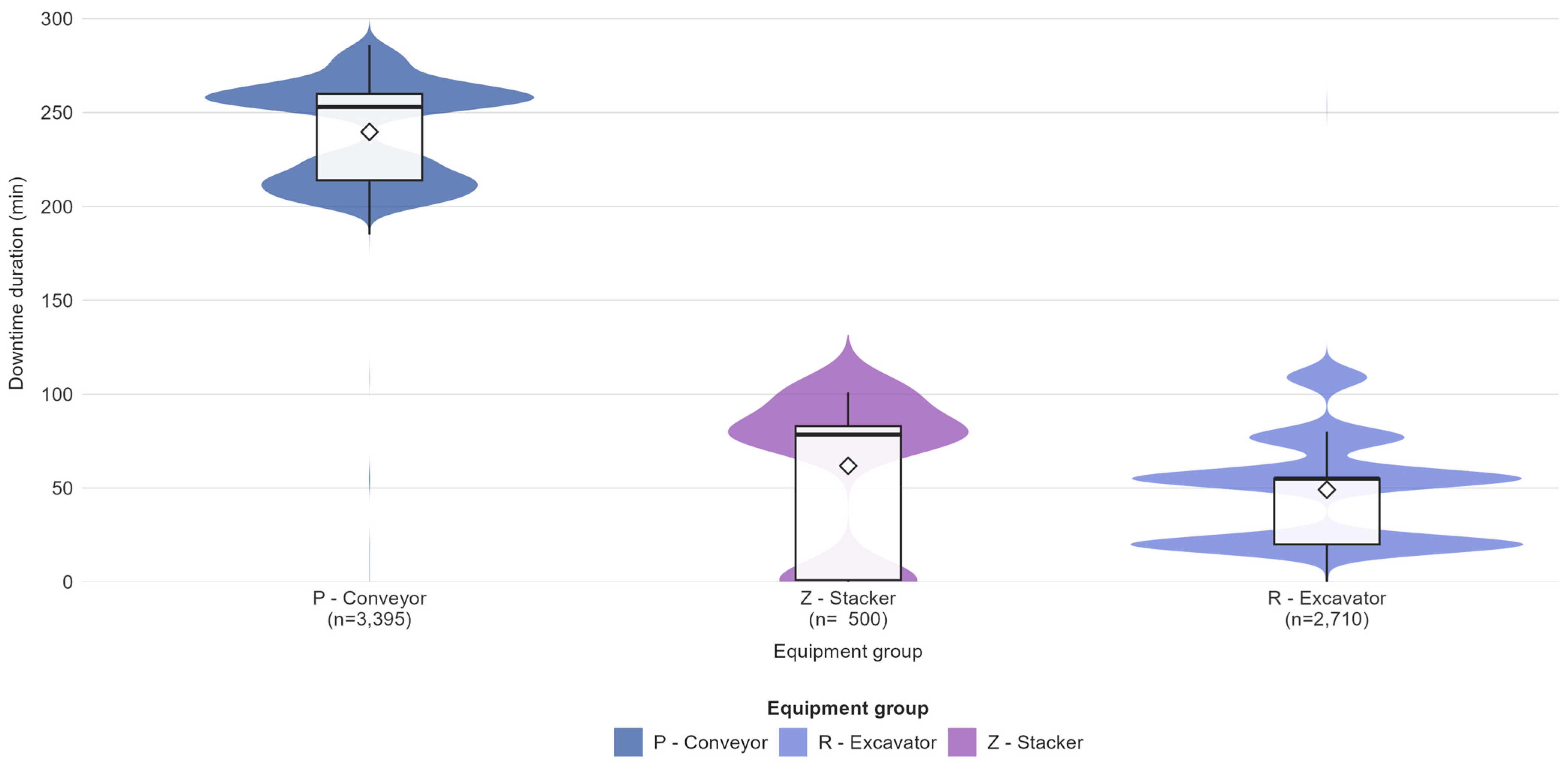
This section evaluates the duration of individual downtime events by equipment group. Because only 72 unique downtime-duration values were identified and the ten most frequent values accounted for 55.41% of all events, the distribution exhibits a heap-like structure. Therefore, the results are better-interpreted using medians, percentile ranges and graphical distribution, rather than the arithmetic mean alone. The distribution and severity of downtime duration by equipment group are shown in Figure 4.

The results reveal clear differences in the severity of downtime. The highest event duration was observed for P–Conveyor, with a median of 253 min and a mean of 239.71 min. This confirms that conveyors dominate not only in event frequency and cumulative downtime, but also in the duration of individual downtime events. R–Excavator showed the lowest typical severity, with a median of 55 min and a mean of 49.13 min. Z–Stacker occupied an intermediate position, with a median of 78.5 min and a mean of 61.84 min, while also showing a more variable distribution.

3.4. Statistical Comparison of Downtime Duration by Equipment Group

A non-parametric Kruskal–Wallis test was used to verify whether downtime duration differed among the analysed equipment groups. This procedure was selected because the downtime duration exhibited a discrete, non-normal, and heaped empirical distribution. The complete dataset contained 6605 records; however, 10 zero-duration records were excluded from the inferential tests because they did not represent positive equipment unavailability time. Therefore, the Kruskal–Wallis test was performed on 6595 events.

The test confirmed statistically significant differences among equipment groups, H = 4983.49, df = 2, p < 0.001. The effect size, epsilon squared = 0.756, indicates a large group effect, meaning that the differences among conveyors, excavators and stackers were not only statistically significant but also operationally substantial.

To identify the specific differences between equipment groups, pairwise Wilcoxon rank-sum tests with Holm correction were subsequently applied. The results are reported in

Table 4. Pairwise Wilcoxon post hoc comparisons of downtime duration.

Comparison	Median Group 1 (min)	Median Group 2 (min)	Median Difference (min)	Adjusted p-Value	Rank-Biserial r	Direction
P–Conveyor vs. R–Excavator	253	55	198	<0.001	0.998	P–Conveyor higher
P–Conveyor vs. Z–Stacker	253	80	173	<0.001	0.998	P–Conveyor higher
R–Excavator vs. Z–Stacker	55	80	−25	<0.001	−0.284	Z–Stacker higher

Source: Own processing in RStudio, R version 4.5.2. Holm correction was applied to p-values.

.

All pairwise comparisons remained statistically significant after Holm correction. The largest difference was observed between P–Conveyor and R–Excavator, with a median difference of 198 min and a rank-biserial correlation of 0.998. P–Conveyor also showed substantially higher downtime duration than Z–Stacker. The comparison between R–Excavator and Z–Stacker was statistically significant, but the effect size was smaller.

These results confirm that the analysed equipment groups should not be treated as operationally equivalent. The significant differences in downtime duration support the use of equipment-specific parameters in the Monte Carlo model.

3.5. Failure-Type Concentration and Pareto Structure

This part of the analysis evaluates whether cumulative downtime was evenly distributed across fault types or concentrated in a limited set of dominant failure modes. Before aggregation, the raw operational fault labels were standardised into professional English fault-type names to ensure terminological consistency. This step is important because equipment-level summaries show where downtime occurs, but they do not identify which specific technical faults to target in maintenance interventions.

The results reported in

Table 5. Top fault types by cumulative downtime.

Rank	Fault Type	Events (n)	Events (%)	Downtime (h)	Downtime (%)	Cumulative Downtime (%)
1	Material Collapse	2485	37.62	6304.97	38.69	38.69
2	Belt Slip	826	12.51	2784.38	17.08	55.77
3	Belt Misalignment	1143	17.31	1763.90	10.82	66.59
4	Belt Run-Off	305	4.62	1092.55	6.70	73.30
5	Other Technical Fault	625	9.46	952.63	5.85	79.14
6	Belt Tear	260	3.94	942.33	5.78	84.92
7	Motor Failure	143	2.17	542.97	3.33	88.25
8	Transfer Chute Spillage	122	1.85	517.10	3.17	91.43
9	Travel Mechanism Failure	278	4.21	318.78	1.96	93.38
10	Power Transmission Failure	89	1.35	273.98	1.68	95.06

Source: Own processing in RStudio, R version 4.5.2.

confirm a strong concentration of downtime burden in a small number of fault types. The most important fault type was Material Collapse, which accounted for 2485 events and 6304.97 h of downtime. This fault type represented 37.62% of all events and 38.69% of cumulative downtime. The second most important fault type was Belt Slip, contributing 17.08% of the total downtime, followed by Belt Misalignment at 10.82%.

The cumulative structure shows a clear Pareto effect. The top three fault types explained 66.59% of total downtime; the top five, 79.14%; and the top ten, 95.06%. This confirms that downtime burden was concentrated in a narrow set of recurrent and operationally significant failure modes. From a maintenance perspective, prioritisation should therefore focus mainly on material-collapse-related failures and belt-system faults.

3.6. Equipment–Fault Combinations as Maintenance Targets

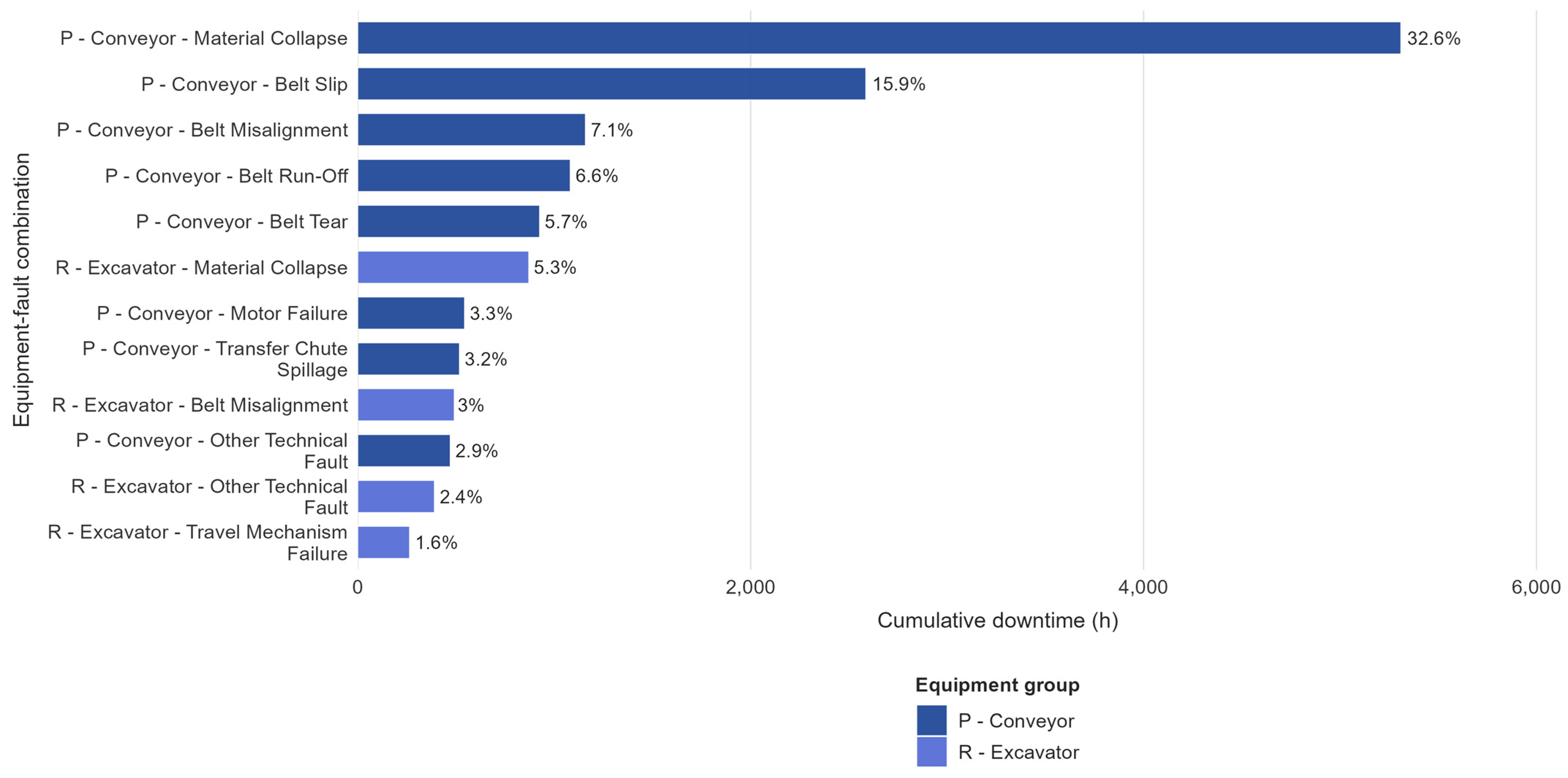
This section combines the equipment group and fault type into a single analytical unit. From a maintenance perspective, this approach is more actionable than evaluating equipment groups or fault types separately, because it identifies which specific combinations generate the greatest downtime burden. The top equipment–fault combinations by cumulative downtime are shown in Figure 5.

The results show that the most critical combination was P–Conveyor–Material Collapse, which alone accounted for 5309.37 h of downtime, representing 32.58% of total system downtime. The second most important combination was P–Conveyor–Belt Slip, contributing 15.87%, followed by P–Conveyor–Belt Misalignment (7.11%) and P–Conveyor–Belt Run-Off (6.63%). The top five combinations already accounted for 67.86% of total downtime, confirming a very high concentration of the downtime burden.

It is also evident that the dominant combinations were mainly associated with conveyors. Excavators appeared among the leading combinations only in a few cases, particularly R–Excavator–Material Collapse and R–Excavator–Belt Misalignment, but their contribution to total downtime was substantially lower.

These findings confirm that maintenance prioritisation should be based on equipment–fault combinations rather than on equipment groups or fault types separately. This combination-level perspective provides the direct empirical bridge between the descriptive downtime analysis and the subsequent evaluation using the Energy–Economic Impact Index.

3.7. Temporal Development of Downtime

This section evaluates whether the burden of downtime remained stable over the observation period or was concentrated in specific years. The annual aggregates show substantial interannual variability in both event frequency and cumulative downtime. The highest cumulative downtime was recorded in 2025, reaching 2881.47 h, representing 17.68% of the total downtime over the full period. The same year also recorded the highest number of downtime events, totalling 1180. By contrast, the lowest annual downtime was observed in 2023, reaching 1219.33 h. The annual development of downtime frequency and cumulative downtime is summarised in

Table 6. Annual development of downtime frequency and cumulative downtime.

Year	Events (n)	Downtime (h)	Downtime (%)	YoY Downtime Change (%)	Median Duration (min)	P95 Duration (min)
2017	634	1582.38	9.71	-	201	265.35
2018	783	2166.70	13.29	36.93	211	271.00
2019	720	1671.25	10.25	−22.87	80	268.00
2020	810	2107.92	12.93	26.13	207	265.55
2021	673	1388.60	8.52	−34.12	55	258.00
2022	538	1267.88	7.78	−8.69	203	262.00
2023	544	1219.33	7.48	−3.83	101	260.00
2024	723	2012.63	12.35	65.06	214	282.00
2025	1180	2881.47	17.68	43.17	109	279.00

Source: Own processing in RStudio, R version 4.5.2.

.

The results indicate that the development of downtime cannot be interpreted as a stable annual average. The strongest year-on-year increase in cumulative downtime occurred in 2024, with a 65.06% rise. Another strong increase was recorded in 2025, reaching 43.17%. The largest year-on-year decrease occurred in 2021, when cumulative downtime declined by 34.12%. These changes indicate a temporally unstable process of downtime.

The temporal trend diagnostics for the annual downtime indicators are summarised in

Table 7. Temporal trend diagnostics for annual downtime indicators.

Indicator	Kendall Tau	p-Value	Sen Slope Per Year	Interpretation
Annual cumulative downtime	−0.056	0.835	−24.75 h/year	decreasing, not statistically significant
Annual event frequency	0.111	0.677	7.88 events/year	increasing, not statistically significant

Source: Own processing in RStudio, R version 4.5.2. Kendall tau and Sen slope were calculated from annual aggregates.

. The trend diagnostics confirmed that no statistically significant monotonic long-term trend could be identified. For annual cumulative downtime, Kendall’s tau was −0.056 (p = 0.835), and the Sen slope was −24.75 h/year. This indicates a slight decrease, but the trend is not statistically significant. For annual event frequency, Kendall’s tau was 0.111 (p = 0.677), and the Sen slope was 7.88 events/year, indicating a slight but statistically non-significant upward trend.

Therefore, the temporal development of downtime should be interpreted primarily as evidence of interannual variability and concentration of downtime burden in specific periods, rather than as evidence of a clear long-term increase or decrease. This result further supports the use of a probabilistic modelling approach, because the historical downtime process does not follow a stable temporal trajectory suitable for simple deterministic extrapolation.

3.8. Monte Carlo Energy-Service, Production and Economic Impact

This section transforms observed downtime into probabilistic estimates of energy-service unavailability, production-loss equivalent and economic impact. Because the primary downtime dataset did not contain directly measured equipment power demand, load factor, handling capacity or unit economic values, the Monte Carlo outputs should be interpreted as modelled interval-based impact estimates, rather than directly measured electricity consumption or realised accounting losses. The equipment-level Monte Carlo impact results are summarised in

Table 8. Equipment-level Monte Carlo impact summary.

Equipment Group	Events (n)	Observed Downtime (h)	Energy-Service Loss P50 (MWh)	Production Loss P50 (kt)	Economic Loss P5–P50–P95 (million EUR)	Median Economic Share (%)
R–Excavator	2710	2219.03	1111.67	3707.29	27.77–82.86–195.97	39.56
P–Conveyor	3395	13,563.83	2922.30	3445.69	33.22–77.43–150.55	36.96
Z–Stacker	500	515.30	256.75	1831.33	13.34–40.91–88.91	19.53

Source: Own processing in RStudio, R version 4.5.2.

.

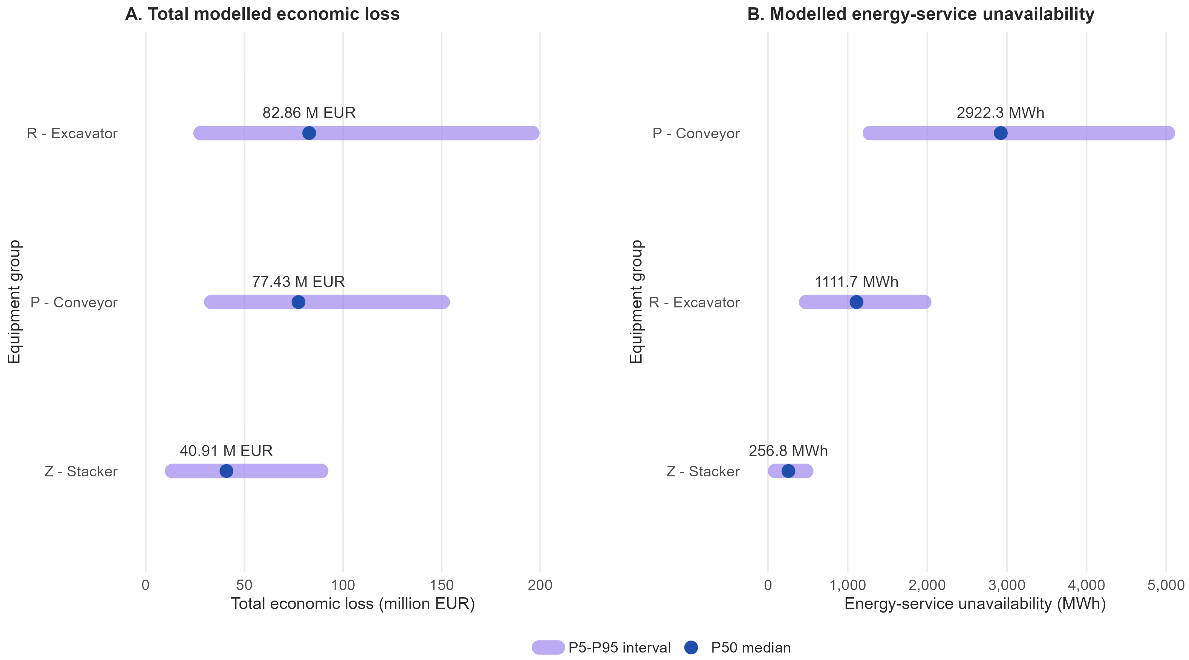
At the equipment level, the highest median economic impact was modelled for R–Excavator, at approximately EUR 82.86 million, representing 39.56% of the median system-level economic loss. Although conveyors had the longest observed downtime, their median economic impact was slightly lower, at EUR 77.43 million. This difference shows that the economic result is determined not only by the duration of downtime but also by the assumed handling capacity and the value of lost production. The highest median energy-service loss was modelled for P–Conveyor, reaching 2922.30 MWh. The highest median production-loss equivalent was estimated for R–Excavator, reaching 3707.29 kt. The system-level Monte Carlo impact summary is presented in

Table 9. System-level Monte Carlo impact summary.

Indicator	P5	P50	P95	Unit
Energy-service loss	2557.52	4338.60	6510.23	MWh
Production-loss equivalent	5686.48	9279.19	13,641.90	kt
Energy-cost component	0.45	0.78	1.22	million EUR
Production-loss cost	107.63	208.66	377.50	million EUR
Total economic loss	108.45	209.48	378.47	million EUR

Source: Own processing in RStudio, R version 4.5.2.

.

At the system level, the median modelled energy-service loss reached 4338.60 MWh, while the median production-loss equivalent reached 9279.19 kt. The total median economic loss was estimated at EUR 209.48 million, with a P5–P95 interval of EUR 108.45–378.47 million. The width of this interval reflects the sensitivity of the final estimate to uncertain technical and economic inputs.

A key result is that the total economic loss was dominated by the production-loss component. The median production-loss cost reached EUR 208.66 million, whereas the median energy-cost component was only EUR 0.78 million. This means that the main economic importance of downtime is not the value of unavailable energy service itself, but the production capacity that becomes unavailable during equipment stoppage. The Monte Carlo uncertainty intervals by equipment group are shown in Figure 6.

The results confirm that maintenance priorities cannot be determined only from event frequency or cumulative downtime. Equipment with fewer events may still have a greater economic impact if it is associated with higher handling capacity or a higher production-loss value. The Monte Carlo stage, therefore, extends the descriptive downtime analysis by adding dimensions of energy service, production, and economic impact.

3.9. Energy–Economic Impact Index for Maintenance Prioritisation

An integrated evaluation of downtime requires the simultaneous consideration of operational frequency, downtime severity, energy-service impact and economic consequences. For this purpose, the Energy–Economic Impact Index (EEII) was applied as a composite prioritisation indicator combining four normalised components: event frequency, cumulative downtime, median modelled energy-service loss, and median modelled total economic loss. The index enables identification of equipment–fault combinations with the highest maintenance priority, as they integrate multiple dimensions of operational risk.

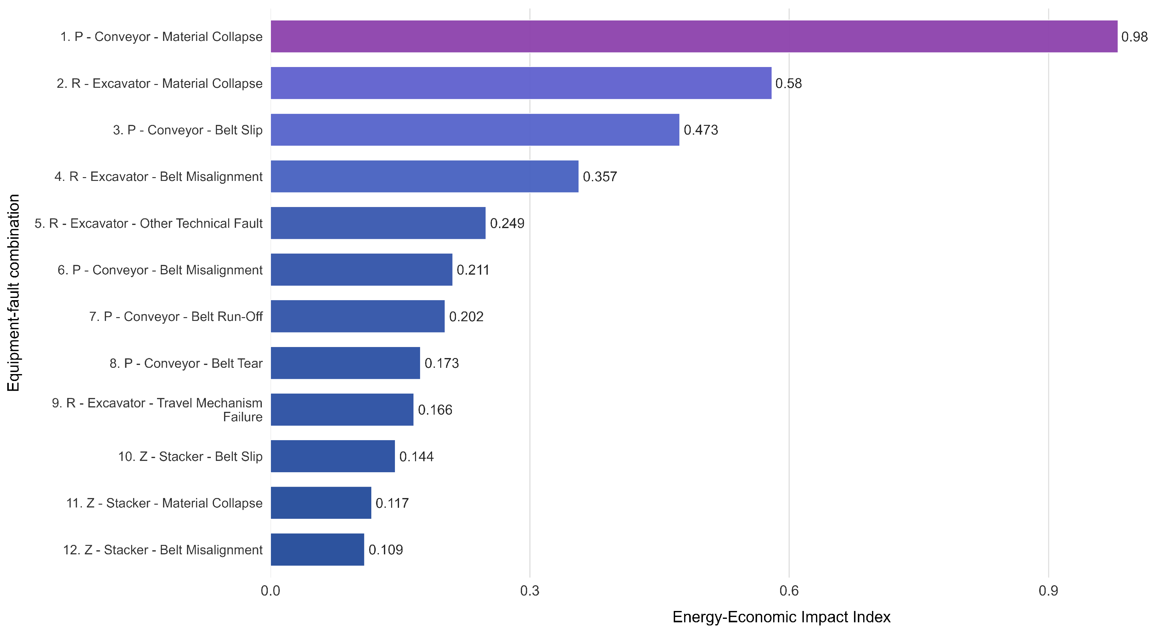
The highest EEII value was obtained by P–Conveyor–Material Collapse (EEII = 0.980), clearly separating it from the remaining maintenance targets. This combination reflects a high event frequency, the highest cumulative downtime, substantial modelled energy-service loss, and a high economic impact. The second-ranked combination was R–Excavator–Material Collapse (EEII = 0.580), followed by P–Conveyor–Belt Slip (EEII = 0.473). This ranking confirms that maintenance priority is shaped by the simultaneous interaction of frequency, downtime severity, energy-service unavailability and economic loss.

The top five EEII-ranked combinations accounted for a dominant share of the integrated system risk profile. From a managerial perspective, this means that maintenance effectiveness may be improved by focusing on a limited set of the highest-risk combinations rather than distributing resources evenly across all recorded fault types.

In the baseline specification of the index, all four components were assigned equal weights (0.25). This setting represents a balanced reference scenario in which no a priori preference is given to failure frequency, cumulative downtime, energy service loss, or economic impact. Under this specification, one equipment–fault combination was classified as very high priority and one as high priority. In applied maintenance planning, the weights can be modified according to management objectives: for example, by assigning a higher weight to economic loss or energy-service unavailability.

The EEII ranking visually confirms the dominant position of P–Conveyor–Material Collapse. The following combinations form a second-priority tier with substantially lower index values. This separation is important because it indicates one system-critical maintenance target and several secondary targets with lower but still relevant impact. The EEII ranking of the leading equipment–fault combinations is shown in Figure 7.

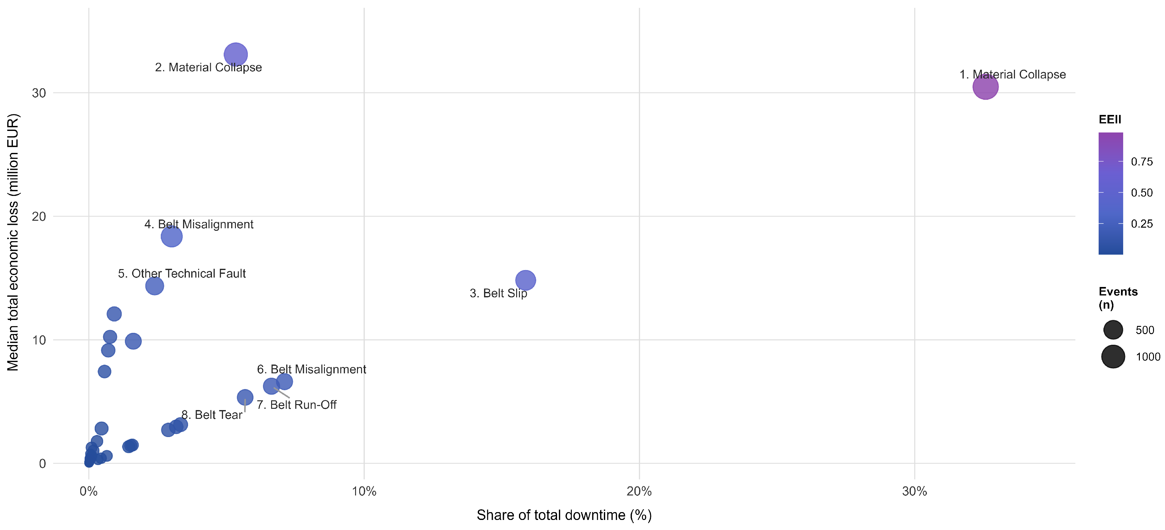
The downtime–economic priority map of the equipment–fault combinations is shown in Figure 8.

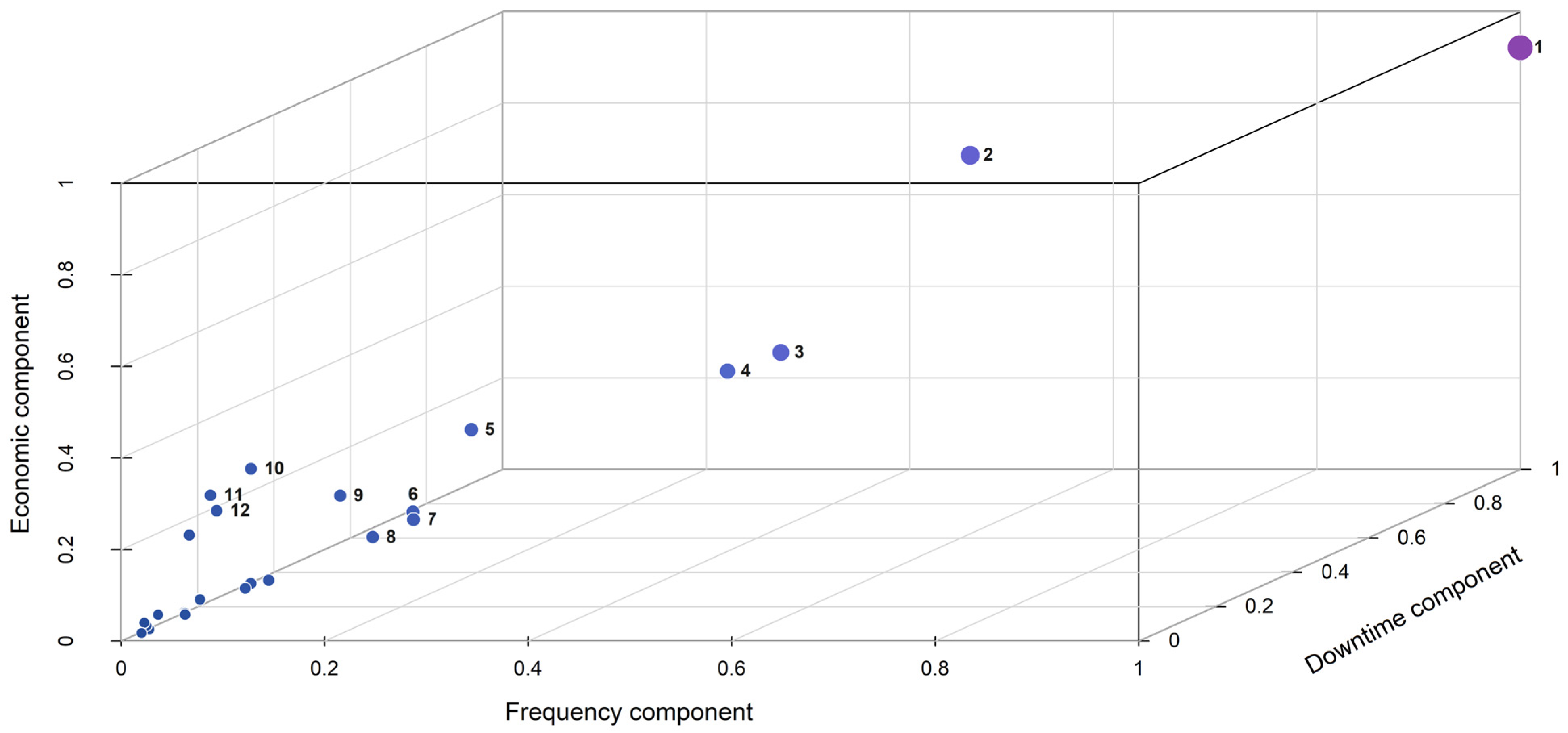
The EEII ranking is further visualised in the three-dimensional priority space shown in Figure 9.

Figure 9. 3D priority space of equipment–fault combinations. Source: Own processing in RStudio, R version 4.5.2. Note: The figure visualises the leading equipment–fault combinations in a three-dimensional space defined by normalised frequency, downtime, and economic impact components. Point colour indicates the relative EEII level, and numeric labels correspond to the EEII ranks reported in Table 10.

Figure 9. 3D priority space of equipment–fault combinations. Source: Own processing in RStudio, R version 4.5.2. Note: The figure visualises the leading equipment–fault combinations in a three-dimensional space defined by normalised frequency, downtime, and economic impact components. Point colour indicates the relative EEII level, and numeric labels correspond to the EEII ranks reported in Table 10.

Table 10. Top maintenance targets ranked by the Energy–Economic Impact Index.

Rank	Equipment Group	Fault Type	Events (n)	Downtime (h)	Energy P50 (MWh)	Economic P50 (million EUR)	EEII	Priority
1	P–Conveyor	Material Collapse	1342	5309.37	1129.18	30.48	0.980	Very high
2	R–Excavator	Material Collapse	1037	870.03	433.41	33.09	0.580	High
3	P–Conveyor	Belt Slip	625	2585.95	555.85	14.82	0.473	Medium
4	R–Excavator	Belt Misalignment	753	490.60	245.97	18.37	0.357	Medium
5	R–Excavator	Other Technical Fault	425	389.52	194.76	14.36	0.249	Low
6	P–Conveyor	Belt Misalignment	275	1158.48	247.87	6.62	0.211	Low
7	P–Conveyor	Belt Run-Off	283	1081.13	230.27	6.25	0.202	Low
8	P–Conveyor	Belt Tear	244	925.20	198.87	5.34	0.173	Low
9	R–Excavator	Travel Mechanism Failure	264	263.08	133.22	9.89	0.166	Low
10	Z–Stacker	Belt Slip	157	150.28	75.02	12.09	0.144	Low

Source: Own processing in RStudio, R version 4.5.2.

Table 10. Top maintenance targets ranked by the Energy–Economic Impact Index.

Rank	Equipment Group	Fault Type	Events (n)	Downtime (h)	Energy P50 (MWh)	Economic P50 (million EUR)	EEII	Priority
1	P–Conveyor	Material Collapse	1342	5309.37	1129.18	30.48	0.980	Very high
2	R–Excavator	Material Collapse	1037	870.03	433.41	33.09	0.580	High
3	P–Conveyor	Belt Slip	625	2585.95	555.85	14.82	0.473	Medium
4	R–Excavator	Belt Misalignment	753	490.60	245.97	18.37	0.357	Medium
5	R–Excavator	Other Technical Fault	425	389.52	194.76	14.36	0.249	Low
6	P–Conveyor	Belt Misalignment	275	1158.48	247.87	6.62	0.211	Low
7	P–Conveyor	Belt Run-Off	283	1081.13	230.27	6.25	0.202	Low
8	P–Conveyor	Belt Tear	244	925.20	198.87	5.34	0.173	Low
9	R–Excavator	Travel Mechanism Failure	264	263.08	133.22	9.89	0.166	Low
10	Z–Stacker	Belt Slip	157	150.28	75.02	12.09	0.144	Low

Source: Own processing in RStudio, R version 4.5.2.

The baseline weighting scheme used for the Energy–Economic Impact Index is presented in

Table 11. Baseline weighting scheme for the Energy–Economic Impact Index.

Component	Symbol	Weight	Interpretation
Failure frequency	F	0.25	Normalised number of downtime events
Downtime severity	D	0.25	Normalised cumulative downtime hours
Energy-service loss	E	0.25	Normalised median Monte Carlo energy-service loss
Economic loss	C	0.25	Normalised median Monte Carlo total economic loss

Source: Own processing in RStudio, R version 4.5.2.

.

3.10. Sensitivity and Robustness Assessment

The probabilistic framework was further evaluated using sensitivity analysis, robustness testing and Monte Carlo stability diagnostics. Standardised regression coefficients were used to identify which input parameters most strongly influenced modelled total economic loss. The EEII ranking was then recalculated under alternative weighting scenarios to test the stability of maintenance priorities. The sensitivity ranking of Monte Carlo input drivers for total economic loss is summarised in

Table 12. Sensitivity ranking of Monte Carlo input drivers for total economic loss.

Rank	Input Driver	Standardised Coefficient	Absolute Coefficient	Direction	p-Value
1	Commodity value	0.709	0.709	Positive	<0.001
2	Capacity R–Excavator	0.546	0.546	Positive	<0.001
3	Capacity P–Conveyor	0.330	0.330	Positive	<0.001
4	Capacity Z–Stacker	0.237	0.237	Positive	<0.001
5	Electricity price	0.004	0.004	Positive	0.021
6	Load factor R–Excavator	0.004	0.004	Positive	0.032
7	Power demand P–Conveyor	0.004	0.004	Positive	0.038
8	Power demand Z–Stacker	−0.004	0.004	Negative	0.045
9	Load factor P–Conveyor	0.002	0.002	Positive	0.271
10	Power demand R–Excavator	−0.001	0.001	Negative	0.491
11	Load factor Z–Stacker	0.000	0.000	Negative	0.860

Source: Own processing in RStudio, R version 4.5.2. Standardised linear regression; adjusted R² = 0.968.

.

The results show that the strongest determinant of total economic loss was the Commodity value, with a standardised coefficient of 0.709. The second strongest factor was Capacity R–Excavator (0.546), followed by Capacity P–Conveyor (0.330) and Capacity Z–Stacker (0.237). By contrast, electricity price, load factor and power-demand parameters had substantially smaller effects. The high adjusted R² value of 0.968 confirms that the selected uncertain inputs explained a large share of the variation in simulated economic loss. Methodologically, this indicates that future model refinement should focus primarily on improving the specification of commodity-value assumptions and equipment-capacity parameters.

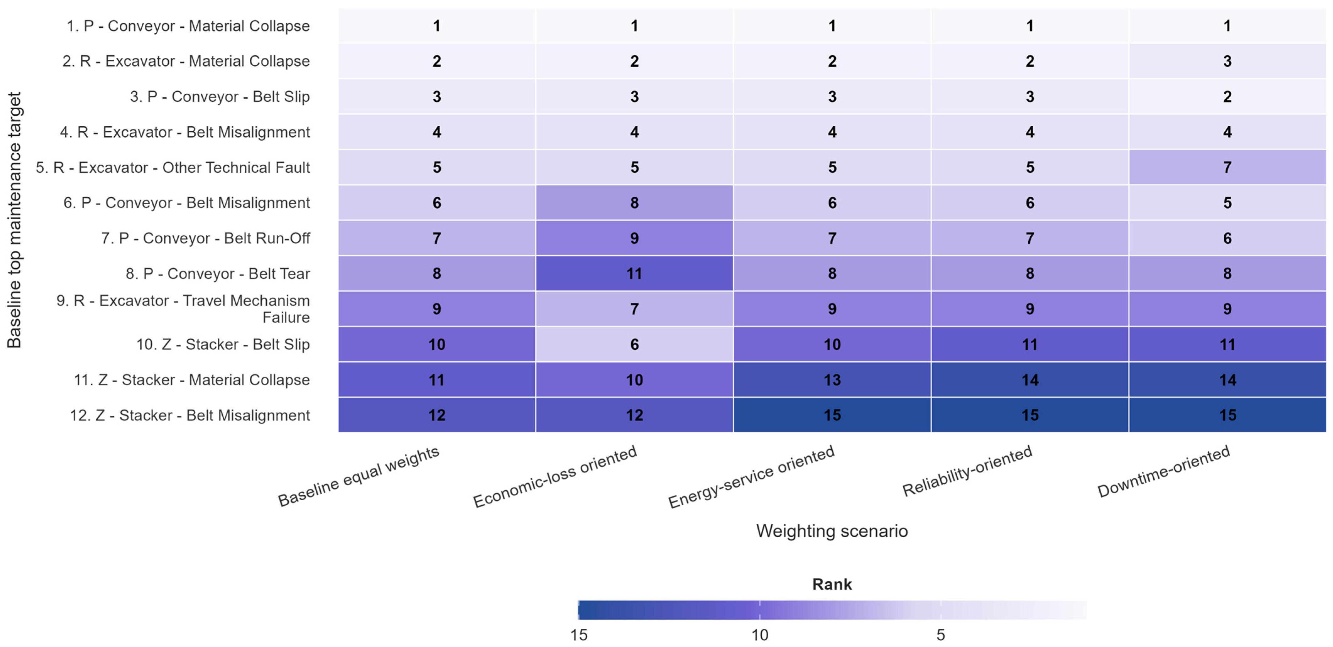
The second part of the assessment examined the robustness of the Energy–Economic Impact Index (EEII) ranking under alternative weighting schemes. In addition to the baseline equal-weight specification, scenarios were evaluated with greater emphasis on economic loss, energy-service loss, reliability-related components and downtime severity. The robustness of EEII-ranked maintenance targets under alternative weighting scenarios is summarised in

Table 13. Robustness of EEII-ranked maintenance targets under alternative weighting scenarios.

Baseline Rank	Equipment–Fault Combination	Baseline EEII	Best Rank	Worst Rank	Mean Rank	Rank SD	Top 10 Occurrence
1	P–Conveyor–Material Collapse	0.980	1	1	1.0	0.00	5/5
2	R–Excavator–Material Collapse	0.580	2	3	2.2	0.45	5/5
3	P–Conveyor–Belt Slip	0.473	2	3	2.8	0.45	5/5
4	R–Excavator–Belt Misalignment	0.357	4	4	4.0	0.00	5/5
5	R–Excavator–Other Technical Fault	0.249	5	7	5.4	0.89	5/5
6	P–Conveyor–Belt Misalignment	0.211	5	8	6.2	1.10	5/5
7	P–Conveyor–Belt Run-Off	0.202	6	9	7.2	1.10	5/5
8	P–Conveyor–Belt Tear	0.173	8	11	8.6	1.34	4/5
9	R–Excavator-Travel Mechanism Failure	0.166	7	9	8.6	0.89	5/5
10	Z–Stacker–Belt Slip	0.144	6	11	9.6	2.07	3/5

Source: Own processing in RStudio, R version 4.5.2.

.

The ranking showed a high degree of stability for the leading maintenance targets. The combination P–Conveyor–Material Collapse retained rank 1 across all scenarios and appeared in the top ten in all five cases. Other key combinations also remained stable, particularly R–Excavator–Material Collapse, P–Conveyor–Belt Slip and R–Excavator–Belt Misalignment. Among the ten highest-ranked targets in the baseline model, eight combinations remained in the top ten across all tested scenarios. This suggests that the leading maintenance priorities are not merely artefacts of the equal-weight specification, but remain robust under changing decision preferences. The rank-stability heatmap of EEII maintenance targets across weighting scenarios is shown in Figure 10.

Monte Carlo stability was evaluated using selected convergence checkpoints in an independent validation run. The purpose of this diagnostic was to verify whether the system-level median estimate remained stable as the number of iterations increased. The final median total economic-loss estimate in the convergence run was EUR 210.25 million, which differs only marginally from the main system-level estimate reported in Table 9. This confirms that the reported Monte Carlo results are not driven by random simulation noise. The Monte Carlo convergence and stability diagnostics are summarised in

Table 14. Monte Carlo convergence and stability diagnostics.

Iterations	Economic P5 (M EUR)	Economic P50 (M EUR)	Economic P95 (M EUR)	Energy P50 (MWh)	P50 Deviation (%)	P95 Deviation (%)
250	104.71	215.20	365.84	4257.43	2.355	3.537
500	112.41	210.59	372.38	4329.73	0.162	1.815
1000	112.42	211.95	372.38	4349.49	0.808	1.815
2500	109.64	209.77	374.72	4345.95	0.227	1.196
5000	110.00	211.17	378.41	4354.77	0.440	0.225
10,000	109.08	210.25	379.26	4336.03	0.000	0.000

Source: Own processing in RStudio, R version 4.5.2.

.

The convergence diagnostics show that the median total economic-loss estimate stabilised as the number of iterations increased. At the last pre-final checkpoint of 5000 iterations, the relative deviation of the median estimate from the final convergence-run value was 0.44%. The difference between the convergence-run median estimate and the main system-level estimate reported in Table 9 is small and does not affect the interpretation of the results. The P5–P95 interval was nevertheless retained because it represents parameter uncertainty, not only simulation variability.

3.11. Correlation Structure and Exploratory Panel Model of Downtime Burden

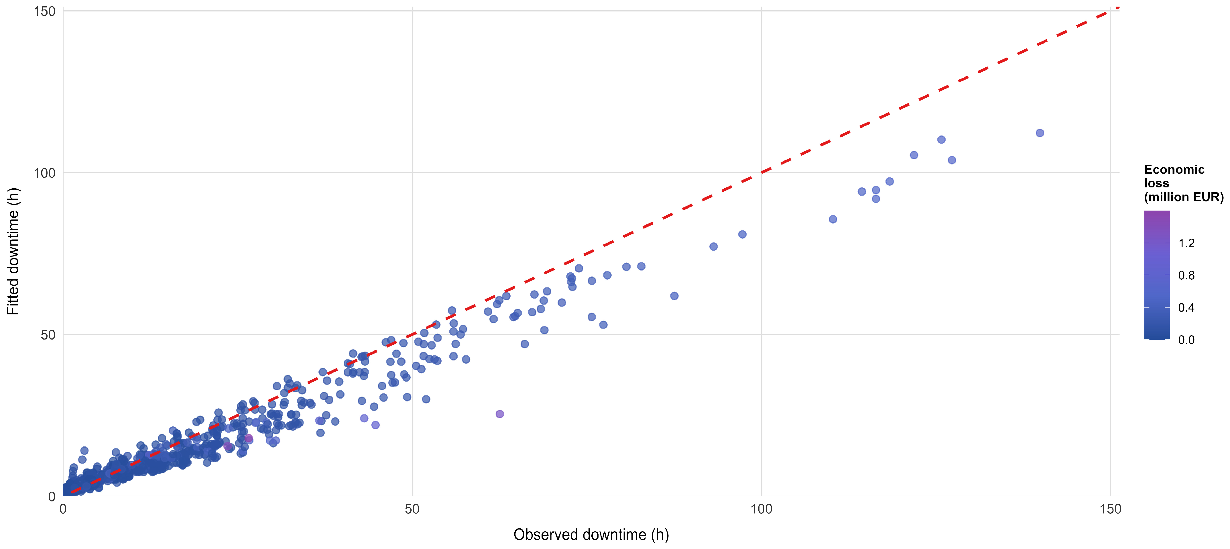
The relationships between operational indicators and modelled energy–economic outputs were further examined using a balanced monthly panel of equipment–fault combinations. The correlation structure confirmed strong positive associations between event frequency, cumulative downtime and modelled impact measures. Event frequency was closely related to cumulative downtime (Spearman ρ = 0.974), while the association between cumulative downtime and modelled economic loss reached ρ = 0.972. An even stronger relationship was observed between modelled energy-service loss and modelled economic loss (ρ = 0.987). These results support the internal coherence of the proposed framework, but they should not be interpreted as independent evidence of causality because the energy and economic indicators are partly derived from observed downtime and interval-based input assumptions. The observed versus fitted panel downtime burden is shown in Figure 11.

The exploratory fixed-effects panel regression further showed that the burden of downtime was significantly associated with both event frequency and the occurrence of longer events. In the model explaining log-transformed downtime burden, the coefficient for log(1 + events) was 0.872, and the coefficient for log(1 + P95 duration) was 0.155, with both predictors being significant at p < 0.001 and within R² = 0.904. In the complementary model of economic loss, cumulative downtime remained the dominant explanatory factor (coefficient = 2.990; p < 0.001), while event frequency also remained significant (coefficient = 2.509; p = 0.017; within R² = 0.744). The comparison of observed and fitted values indicates that the fixed-effects model reproduced the empirical downtime burden reasonably well, although it underestimated at higher observed downtime levels. Therefore, the panel model should be interpreted as an exploratory robustness diagnostic, rather than as causal or precise predictive evidence.

4. Discussion

The results confirm that downtime in a continuous material-handling system should not be interpreted only as a set of isolated operational records or routine maintenance indicators. The downtime burden was strongly concentrated by equipment group, fault type and equipment–fault combination. The most important combination was P–Conveyor–Material Collapse, which accounted for 32.58% of total downtime, while the top five combinations explained 67.86% of cumulative downtime. This directly answers RQ1 and shows that downtime risk in the analysed system was concentrated rather than evenly distributed across all equipment and fault categories. The dominance of conveyor-related failures is also consistent with studies emphasising the operational importance of belt-conveyor reliability in continuous material-handling systems [10,11,12,53,54,55].

A key finding is the distinction between event frequency and actual operational impact. Conveyors dominated cumulative downtime and event-level severity, but the Monte Carlo model showed that excavators may generate a comparable or even higher median economic impact due to their assumed handling capacity and production-loss parameters. This extends the conventional maintenance interpretation of downtime: event counts alone are insufficient. Downtime should be evaluated alongside duration, equipment functionality, capacity assumptions, and the economic value of lost production. This interpretation is consistent with downtime-cost literature, where downtime is understood as a combination of lost output, unused capacity and financial consequences [4,5,26,27,28].

Methodologically, the study demonstrates that historical downtime records can be used to develop a probabilistic decision-support model even when complete technical and economic data are unavailable. RQ2 was addressed by the representing power demand, load factor, handling capacity, electricity price and commodity value through interval-based triangular distributions. These inputs were propagated through 10,000 Monte Carlo iterations and reported using P5–P50–P95 intervals. This approach is more defensible than a deterministic single-point estimate because it explicitly incorporates input uncertainty and reduces the risk of false precision. The modelling strategy is consistent with Monte Carlo applications in the availability, reliability and maintenance assessment of technical and energy systems [1,2,3,20,24,29,30,31,32,35,36].

The Monte Carlo results answer RQ3. At the system level, the median modelled energy-service unavailability reached 4338.60 MWh, the median production-loss equivalent reached 9279.19 kt, and the median total economic loss was EUR 209.48 million. These values show that downtime should be understood not only as technical equipment unavailability but also as an energy-service, production-capacity, and economic-risk problem. However, the energy-related output must not be interpreted as directly metered electricity consumption during downtime. It represents the modelled unavailability of productive energy service, meaning the energy-linked productive capacity that could not be used because the equipment was unavailable. This interpretation connects maintenance analysis to energy efficiency, OEE and production-system performance [14,15,16,17,18,19,37,38,39,40,41].

The main practical contribution is the Energy–Economic Impact Index, which answers RQ4. The highest-ranked maintenance target was P–Conveyor–Material Collapse, with an EEII value of 0.980. The top five EEII targets accounted for 59.18% of the total downtime and approximately 54.65% of median modelled economic loss. This confirms that maintenance priorities should not be determined solely by frequency or cumulative downtime, but by the combined operational, energy-service and economic consequences of downtime. In this sense, the EEII is aligned with TPM, OEE, cost-oriented maintenance and FMEA-based approaches, in which priorities are determined by failure consequences rather than by failure occurrence alone [13,39,44,45].

The sensitivity and convergence analyses strengthen the interpretation of the probabilistic results. Commodity value and equipment-capacity parameters were the strongest drivers of total economic loss, while the electricity price and power demand parameters had a much smaller influence. This indicates that the economic severity of downtime in this system is determined primarily by the value of lost production and handling capacity, rather than by energy costs alone. The convergence diagnostics also confirmed that the Monte Carlo estimates were stable at 10,000 iterations, supporting the robustness of the results for article-level interpretation and decision support.

The study has several limitations. The energy and economic outputs are modelled estimates rather than direct measurements. The primary dataset contained detailed downtime records but did not include event-level power demand, load factor, handling capacity, or internal cost data. Therefore, the results should not be interpreted as accounting losses or measured electricity consumption. They represent probabilistic value-at-risk estimates under the assumption of a defined interval. This limitation was mitigated through transparent input intervals, percentile-based reporting, sensitivity analysis and a consistent distinction between energy-service unavailability and measured electricity use. The panel regression and correlation results should also be interpreted as diagnostic and associative, rather than causal evidence.

Overall, the findings show that historical downtime records can be used for more than retrospective failure description. When combined with interval-based technical and economic assumptions, they enable quantification of energy-service unavailability, production-loss equivalents, and probabilistic economic impact. The main contribution of the study, therefore, lies in integrating reliability, energy-service availability, productive capacity, and economic value into a single decision-support framework. The methodology is transferable to other continuous or quasi-continuous bulk-material systems, such as ports, cement plants, steel production logistics, or bulk terminals, but the numerical inputs must be recalibrated for each industrial context.

5. Conclusions

This study demonstrated that long-term downtime records can be transformed into a probabilistic framework for assessing operational, energy-service and economic impacts in a continuous material-handling system. The results confirmed a strong concentration of downtime burden in a limited number of equipment–fault combinations. The most important combination was P–Conveyor–Material Collapse, which accounted for 32.58% of total downtime, while the top five combinations explained 67.86% of cumulative downtime.

The Monte Carlo simulation enabled the incorporation of uncertain technical and economic inputs through interval-based assumptions. At the system level, the median modelled energy-service unavailability reached 4338.60 MWh, the median production-loss equivalent reached 9279.19 kt, and the median total economic loss reached EUR 209.48 million. These results show that downtime should be evaluated not only as a technical interruption but also as a source of unavailable energy service, lost production capacity, and economic risk.

The main practical output of the study is the Energy–Economic Impact Index, which integrates event frequency, cumulative downtime, modelled energy-service unavailability and economic loss into a single maintenance-prioritisation indicator. The highest priority was assigned to P–Conveyor–Material Collapse, confirming that maintenance decisions should not be based solely on failure counts, but on the combined operational, energy-related and economic consequences of downtime.

The main limitation of the study is that the energy and economic results are modelled estimates rather than directly measured values. Nevertheless, the use of interval-based inputs, percentile reporting, sensitivity analysis, convergence diagnostics and robustness testing reduces the risk of overinterpretation. The proposed framework is therefore suitable as a decision-support tool for industrial systems where detailed downtime records are available, but complete technical and economic measurements are not systematically recorded.

Future research should validate the framework using directly measured equipment power demand, load factors and handling capacities. Further work should also examine cascading dependencies between excavators, conveyors and stackers, incorporate buffer and redundancy effects, and compare the proposed EEII-based prioritisation with maintenance-resource allocation models. Application of the framework to other bulk-material sectors, such as ports, cement plants, steel logistics, and bulk terminals, would help assess its transferability across different equipment structures and economic conditions.