Multi-Scale Estimation of Urban Carbon Emissions Using Nighttime Light Data: A Case Study of Nanjing, China

Abstract

Rapid urbanization and associated greenhouse gas emissions pose severe challenges to global climate goals. Accurately estimating urban carbon emissions at fine administrative scales is a critical prerequisite for spatially differentiated mitigation policies and achieving carbon neutrality. However, while current research has validated the feasibility of using nighttime light (NTL) remote sensing for carbon estimation, most studies predominantly focus on macro scales, paying limited attention to intra-urban spatial heterogeneity and the value of high-resolution imagery. Using Nanjing, China, as a case study, this study examines the optimal scale, model, and data source for estimating urban total carbon emissions. NTL features from NPP/VIIRS and Luojia1-01 imagery were extracted at the district and township levels. Spatial lag and spatial error models were compared, and geographically weighted regression was further applied at the township level. The results show that urban carbon emissions in Nanjing exhibit clear scale effects and spatial non-stationarity. At the township level, the total indicator (TCE-TNLI) better reflects emission expansion in peripheral areas, while the intensity indicator (CI-ANLI) shows better predictive performance and robustness. With high-resolution Luojia1-01 imagery, the intensity model further reduces the effects of pixel saturation and administrative scale differences, achieving better model performance. These findings establish a robust methodological framework for fine-scale urban carbon accounting, demonstrating that integrating high-resolution imagery with intensity-based models is crucial for supporting spatially differentiated low-carbon planning in high-density megacities.

1. Introduction

With the continuous acceleration of global urbanization, climate change characterized by the persistent accumulation of greenhouse gases has become one of the most severe environmental challenges facing humanity [1,2,3]. As the core spatial carriers of human activities and energy consumption, urban areas account for more than 70% of global carbon dioxide emissions [4,5,6]. In the context of the carbon peaking and carbon neutrality goals, accurately quantifying urban total carbon emissions (TCE) and identifying their spatial distribution patterns have become prerequisites for formulating differentiated mitigation policies and supporting low-carbon urban spatial planning [7]. As a megacity in eastern China and an important hub in the Yangtze River Delta urban agglomeration, Nanjing has experienced rapid urban expansion and increasingly intensive human activities, which have exerted profound impacts on regional carbon emission loads [8,9,10]. Therefore, obtaining high-precision and dynamic spatial data on anthropogenic carbon emissions in Nanjing is of urgent practical significance. Enhanced precision in intra-urban carbon estimates enables municipal authorities to transition from macro-level, uniform emission reduction targets toward grid-level, spatially differentiated mitigation interventions. Specifically, accurate fine-scale carbon accounting can mitigate the risk of spatial misallocation of public resources, facilitate targeted low-carbon building retrofits, and provide a quantitative basis for evaluating the localized efficacy of neighborhood-scale environmental policies.

At present, urban carbon emission accounting mainly follows the Intergovernmental Panel on Climate Change (IPCC) methodological framework and can generally be divided into two categories: top-down estimation based on aggregated statistics and bottom-up inventory construction [11,12]. The top-down approach, usually relying on energy balance tables, is highly applicable to macro-level policy assessment; however, it lacks explicit spatial attributes and is therefore insufficient for fine-scale intra-urban management [13,14]. By contrast, bottom-up approaches can better reflect sectoral and local differences in energy use, but they often face major challenges, including limited data accessibility, weak statistical infrastructure, and high time and financial costs [15]. These constraints become particularly pronounced when carbon accounting is conducted at finer administrative levels, such as districts or townships/subdistricts, where detailed energy consumption data are often unavailable [16,17].

Rapid advances in remote sensing have provided a promising alternative for overcoming these limitations in spatialized carbon estimation [18]. Nighttime light imagery can objectively and continuously capture the radiative intensity of human activities on the Earth’s surface, and has been widely shown to be strongly correlated with socioeconomic indicators, electricity consumption, and anthropogenic carbon emissions [19,20,21]. In terms of data development, early studies mainly relied on DMSP-OLS imagery with a spatial resolution of approximately 1000 m, whereas most recent NTL-based carbon estimation studies use NPP/VIIRS data with a spatial resolution of about 500 m, which benefits from improved radiometric resolution and reduced saturation effects [22]. More recently, a new generation of high-resolution NTL satellites, such as Luojia 1-01 with a spatial resolution of about 130 m, has substantially improved the ability to detect complex intra-urban structures and the physical boundaries of human activities [23,24]. This creates new opportunities for analyzing the spatial network characteristics of urban anthropogenic carbon emissions at finer scales.

The modeling logic of NTL-based carbon estimation has also evolved from simple macro-level association analysis toward finer spatial decomposition. Early studies mainly focused on testing the statistical relationships between low-resolution imagery, such as DMSP-OLS, and socioeconomic or energy-consumption indicators at the national or provincial scales, with ordinary least squares (OLS) regression as the dominant analytical approach [21,25]. As the spatial scale of analysis becomes finer, however, traditional models that ignore spatial dependence and spatial heterogeneity often produce biased parameter estimates and fail to capture the complexity of intra-urban carbon emission patterns [26,27]. To address this issue, spatial econometric models, such as the spatial lag model (SLM) and spatial error model (SEM), as well as local regression methods such as geographically weighted regression (GWR), have gradually become important tools for revealing the spatial non-stationarity of carbon emissions [26,27,28]. At the same time, the application of NTL data has expanded from macro-scale index fitting to the refined delineation of physical boundaries and morphological structures of human activities using high-resolution imagery [23]. This methodological shift not only improves estimation robustness, but also offers new perspectives for exploring the spatiotemporal dynamics of carbon sources within high-density cities [24].

Despite these advances, several important gaps remain in existing NTL-based carbon emission studies. First, most previous research has focused on national, provincial, or large urban agglomeration scales, while the estimation performance and applicability of NTL data at finer scales, such as districts and townships, remain insufficiently understood [29]. Second, in typical high-density megacities, the driving mechanisms of carbon emissions are characterized by strong spatial heterogeneity and non-stationarity. Global regression models often fail to capture such local variations [30,31], whereas local models such as GWR have shown clear advantages in revealing spatially differentiated relationships [32]. More importantly, the relationship between spatial resolution and estimation accuracy is not necessarily linearly positive across all scales [33]. Although high-resolution imagery may introduce disturbances from non-productive light sources, such as minor road networks and scattered infrastructure lighting, which can reduce goodness of fit at broader scales [34], it still has clear advantages over coarse-resolution data in suppressing background noise, delineating complex human activity boundaries, and supporting more detailed spatial analysis [35]. However, the deeper analytical value of high-resolution imagery and its anti-interference performance in multi-scale carbon estimation have not yet been systematically examined.

To address these gaps, this study takes Nanjing as the empirical case and integrates two open-access NTL datasets—NPP/VIIRS and high-resolution Luojia 1-01 imagery—to construct a multi-scale framework for carbon emission estimation from the district to the township level. Spatial lag, spatial error, and geographically weighted regression (GWR) models are systematically introduced to account for spatial dependence and identify the optimal combination of spatial scale, model, and data source. To provide rigorous, question-driven guidance for this empirical investigation, this study explicitly addresses how administrative scale transitions from the district to the township level modulate spatial non-stationarity, whether intensity-based carbon indicators exhibit superior statistical robustness over total-value metrics in fine-scale spatial regressions, and whether high-resolution imagery can effectively mitigate pixel saturation in high-density urban cores to optimize intensity-based estimation. Resolving these interconnected inquiries is expected to improve the understanding of spatial association patterns of carbon emissions in complex urban environments, thereby providing a robust methodological foundation for granular urban carbon accounting and targeted low-carbon spatial governance.

2. Materials and Methods

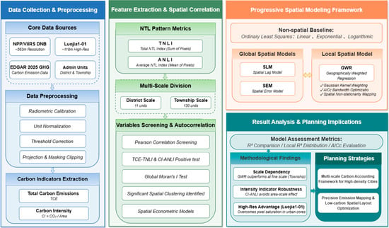
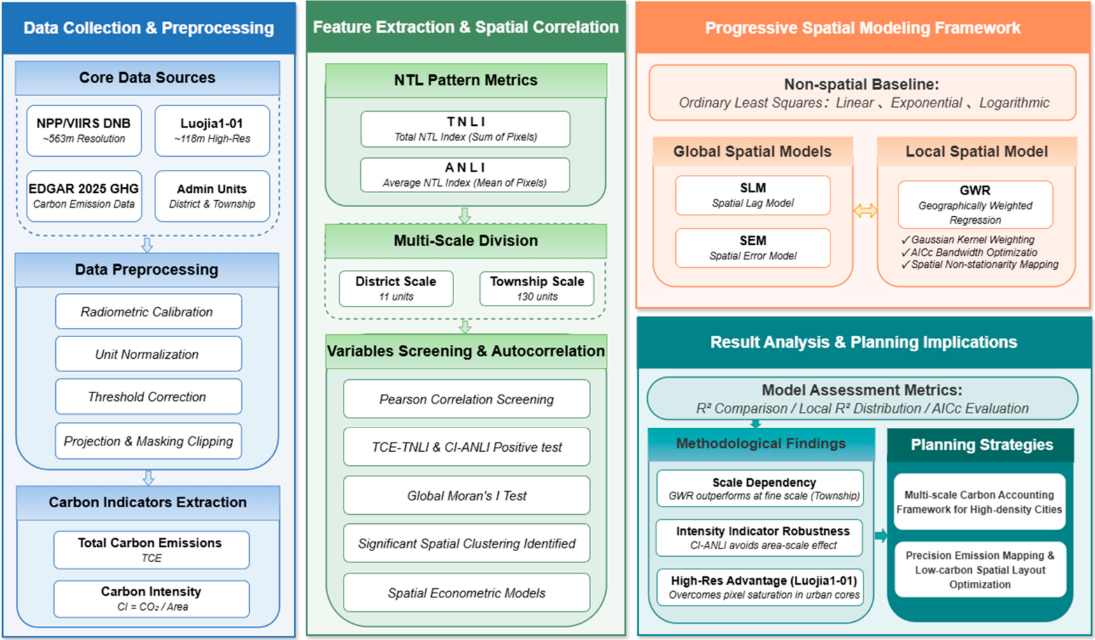
This study investigates the spatial distribution characteristics and multi-scale estimation models of total carbon emissions in Nanjing, based on multi-source nighttime light remote sensing imagery and total carbon emission data (Figure 1). A progressive analytical framework is adopted. First, the study focuses on data preprocessing and feature extraction. After correcting NPP/VIIRS and Luojia-1 imagery, nighttime light indicators, total carbon emissions, and carbon intensity are extracted at both district and township scales, laying a foundation for subsequent analysis. Furthermore, to better understand the spatial dependence of total carbon emissions, Moran’s I is employed to examine the spatial clustering characteristics of the variables [36,37]. On this basis, a spatial modeling framework is constructed, comparing non-spatial baseline models with global spatial models (SLM and SEM), and incorporating geographically weighted regression to reveal local spatial non-stationarity in carbon emissions. Finally, multiple evaluation metrics (R² and AICc) are used to validate and analyze the models, providing scientific support for constructing a multi-scale carbon accounting system and optimizing low-carbon spatial layouts in high-density cities.

Figure 1. Research framework.

2.1. Research Area

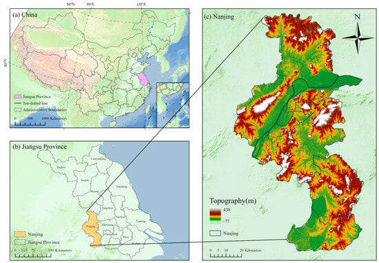
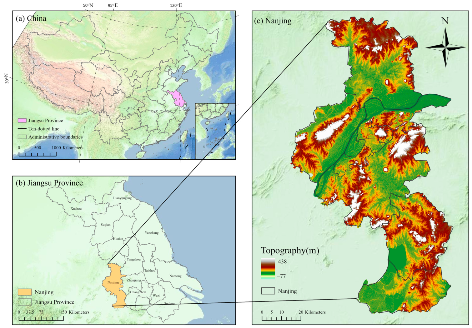
To minimize the influence of external factors such as non-building light sources while ensuring data availability and regional representativeness, Nanjing was selected as the study area. Nanjing (31°14′–32°37′ N, 118°22′–119°14′ E), located in the middle of the lower reaches of the Yangtze River, is the capital of Jiangsu Province and an important central city in the Yangtze River Delta urban agglomeration, with a total area of 6587.04 km² (Figure 2). As of December 2024, Nanjing administers 11 districts, including Xuanwu, Qinhuai, Jianye, Gulou, Qixia, Yuhuatai, Jiangning, Pukou, Liuhe, Lishui, and Gaochun. The city has an urbanization rate of 87.3%. Its urban structure is characterized by a densely built central area with concentrated public and commercial buildings, suburban zones dominated by new residential communities and industrial functional areas, and outer suburban areas mainly composed of village construction land and ecological space. As a result, significant spatial differences exist in building scale, energy-use intensity, and human activity patterns [10,38]. As a megacity in eastern China with a high level of urbanization and large overall energy consumption, Nanjing has a relatively high share of building-sector energy use in total urban energy consumption, making it a representative case for fine-scale carbon emission research [39,40,41]. Under the carbon peaking and carbon neutrality goals and the broader agenda of low-carbon urban development, there is a clear practical need to examine the spatial accounting, scale effects, and model application of carbon emissions in this region. In addition, Nanjing has complete administrative units, clear spatial boundaries, and relatively sound data support, providing a stable and reliable empirical basis for carbon emission estimation and multi-model comparison at both the district and township scales [38].

Figure 2. Location of the research region: (a) China; (b) Jiangsu province; (c) Nanjing.

2.2. Data Source and Preprocessing

This study focuses on regression modeling of the relationship between nighttime light (NTL) data and carbon emissions in Nanjing under different administrative divisions. The datasets used in this study can be divided into two main categories. First, to evaluate estimation performance across spatial scales, carbon emission data at different administrative levels were required. The carbon emission data for Nanjing were obtained from the EDGAR_2025_GHG database (https://edgar.jrc.ec.europa.eu/dataset_ghg2025, accessed on 28 February 2026) and spatialized to two administrative scales: the district level and the township level. At the district level, Nanjing comprises 11 municipal districts. At the township level, these districts are further subdivided into 130 township-level units, whose boundaries are derived from OpenStreetMap (https://www.openstreetmap.org, accessed on 1 March 2026).

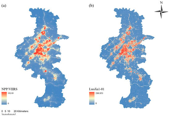
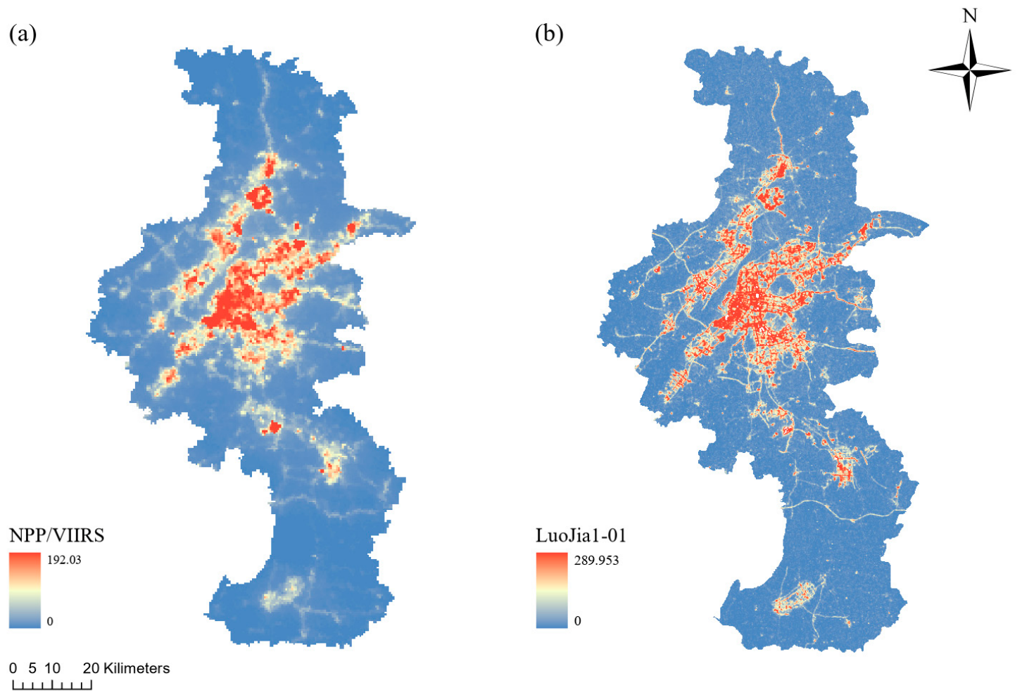
In addition, NTL data were collected to compare the performance of different estimation models. Two NTL datasets were used in this study: NPP/VIIRS and Luojia 1-01 imagery (Figure 3). The characteristics and sources of these two remote sensing datasets are as follows:

Figure 3. (a) NPP/VIIRS; (b) Luojia1-01.

(a)

NPP/VIIRS DNB provides monthly cloud-free composite nighttime light imagery with a spatial resolution of approximately 563.78 m. The data were obtained from the Earth Observation Group (https://eogdata.mines.edu/products/vnl/, accessed on 10 March 2026).

(b)

Luojia 1-01 provides high-resolution monthly nighttime light imagery with a spatial resolution of 117.62 m. Since June 2018, these data have been freely available from the Hubei Data and Application Center (http://59.175.109.173:8888/app/login.html, accessed on 10 March 2026).

This study used NTL satellite imagery covering Nanjing for the year 2018. All datasets were projected to the same coordinate system, WGS 1984 UTM Zone 49N.

Due to data transmission and storage constraints, the downloaded Luojia 1-01 imagery does not directly provide usable grayscale values and therefore requires further conversion before analysis [42]. The recommended preprocessing procedure for Luojia 1-01 NTL data is to calculate radiance as follows:

$$\mathrm{L} = \mathrm{D}{\mathrm{N}}^{3/2}\cdot 10^{-10}$$

(1)

where DN is the digital number recorded for each pixel, and L is the radiometrically calibrated radiance, expressed in W/(m²⋅sr⋅μm) This radiometric calibration converts the original int32 values into physically meaningful floating-point data.

To ensure comparability between Luojia 1-01 and NPP-VIIRS data, the calibrated Luojia 1-01 radiance was further converted to a consistent unit and magnitude using the following equation:

$${\mathrm{L}}^{\mathrm{*}}=\mathrm{L}\times 0.52\times 10^5$$

(2)

where L is the calibrated radiance of Luojia 1-01, and L^* is the normalized radiance with the same unit as NPP-VIIRS, i.e., nW/(cm²⋅sr).

For NPP-VIIRS imagery, no additional radiometric calibration was required because official system-level preprocessing has already been completed. However, the dataset does not completely remove aurora, fires, boats, or other abnormal light sources during compositing, which may result in unusually high pixel values. In addition, the compositing algorithm may generate a small number of negative values [43,44]. To remove residual outliers and negative pixels, threshold correction was applied. Following previous studies, the minimum threshold was set to 0 and the maximum threshold to 350 [45]. Preliminary spatial checks confirmed that within the urban context of Nanjing, normal infrastructure and commercial lighting do not exceed this upper bound, ensuring that the threshold strictly filters anomalous extreme values without truncating legitimate urban signals. The correction rule is defined as:

$$\mathrm{N}\mathrm{T}\mathrm{L}=\{\begin{array}{l}0 \mathrm{L}\mathrm{i}\mathrm{g}\mathrm{h}\mathrm{t}\mathrm{V}\mathrm{a}\mathrm{l}\mathrm{u}\mathrm{e}<0\\ \mathrm{L}\mathrm{i}\mathrm{g}\mathrm{h}\mathrm{t}\mathrm{V}\mathrm{a}\mathrm{l}\mathrm{u}\mathrm{e} 0<\mathrm{L}\mathrm{i}\mathrm{g}\mathrm{h}\mathrm{t}\mathrm{V}\mathrm{a}\mathrm{l}\mathrm{u}\mathrm{e}<\mathrm{M}\mathrm{a}\mathrm{x}\mathrm{V}\mathrm{l}\mathrm{u}\mathrm{e}\\ \mathrm{M}\mathrm{a}\mathrm{x}\mathrm{V}\mathrm{a}\mathrm{l}\mathrm{u}\mathrm{e} \mathrm{L}\mathrm{i}\mathrm{g}\mathrm{h}\mathrm{t}\mathrm{V}\mathrm{a}\mathrm{l}\mathrm{u}\mathrm{e}>\mathrm{M}\mathrm{a}\mathrm{x}\mathrm{V}\mathrm{l}\mathrm{u}\mathrm{e}\end{array}$$

(3)

This thresholding procedure effectively removes abnormal values and improves data quality. Afterward, the NPP-VIIRS NTL data were also projected and clipped to the study area boundary to maintain spatial consistency with the Luojia 1-01 data. After these preprocessing steps, the two NTL datasets with different spatial resolutions could be compared and validated under a unified physical measurement framework, providing a reliable basis for subsequent multi-scale feature extraction.

As the dependent variable for the subsequent multi-scale spatial regression analysis, carbon emissions in each spatial unit of Nanjing were also quantified. In addition to total carbon emissions, this study further introduced a carbon intensity indicator because substantial differences in area exist among districts and street-level units. Relying only on total emissions may therefore fail to accurately reflect the actual emission level within each unit. To reduce the scale effect caused by differences in administrative area and to better evaluate carbon emissions and energy-use efficiency per unit area, carbon intensity was calculated as follows [46]:

$${\mathrm{b}}_{\mathrm{i}\mathrm{j}}={\displaystyle \frac{{\mathrm{B}}_{\mathrm{i}\mathrm{j}}}{{\mathrm{A}}_{\mathrm{i}\mathrm{j}}}}$$

(4)

where b_ij denotes the carbon emission intensity of spatial unit j in region i, B_ij is the total carbon emissions of that unit, and A_ij is the total land area of the corresponding administrative or spatial unit.

Through the above processing, the absolute carbon emissions were transformed into a relative carbon intensity indicator, and the two NTL datasets were standardized under a unified physical basis. This standardization not only provides a reliable reference for evaluating energy-use efficiency across scales, but also establishes a solid data foundation for examining the spatial non-stationarity between NTL indicators and carbon emission metrics and for constructing multi-scale spatial regression models.

2.3. Research Method

2.3.1. Non-Spatial Regression Models

In many previous studies, ordinary least squares has been widely used to establish linear regression models between NTL data and socioeconomic or energy-related variables [47,48]. While machine learning techniques like Random Forest and XGBoost have recently gained popularity for predictive tasks, they often obscure the spatially non-stationary mechanisms underlying total carbon emissions. Furthermore, these data-intensive algorithms are prone to overfitting given the localized sample sizes inherent to this study’s administrative divisions (11 districts and 130 townships). Therefore, this study first constructed three basic regression models, namely linear, logarithmic, and exponential models, to preliminarily explore the fitting relationship between NTL and carbon emissions. The goodness of fit of all models was evaluated using the coefficient of determination ($R^2$).

2.3.2. Spatial Regression Models

In geographic analysis, traditional regression models may perform poorly when spatial autocorrelation exists in the data [49]. Spatial autocorrelation in the residuals indicates that the residuals exhibit systematic patterns related to spatial location [50]. This suggests that the assumption of independence among observations is violated and that important spatial variables may have been omitted. As a result, parameter estimates may be biased and statistical inference may be misleading, preventing the model from adequately explaining the contribution of explanatory variables to the response variable [51]. Compared with non-spatial regression models, which may produce non-randomly distributed residuals, spatial regression models address residual autocorrelation by incorporating a specific spatial weight matrix, such as inverse-distance or nearest-neighbor weights [52]. Spatial econometric models, including the spatial lag model, the spatial error model, and geographically weighted regression, are commonly used to capture the spatial effects of autocorrelation, spatial stationarity, and heterogeneity in feature distributions [53].

2.3.3. Spatial Lag Model

The SLM assumes that the dependent variable is affected not only by local explanatory variables but also directly by the dependent variables of neighboring areas [54]. This model explicitly incorporates spatial dependence into the regression structure, which can be expressed as:

$$y_i=x_i\beta +\rho Wyi+{\epsilon }_i$$

(5)

where $y_i$ is the observed dependent variable at location $i$; $x_i$ is the matrix of explanatory variables; $\beta$ is the vector of regression coefficients; $\rho$ is the spatial autoregressive coefficient; $W$ is the spatial weight matrix describing the adjacency and interaction among spatial units; and ${\epsilon }_i$ is the random error term.

2.3.4. Spatial Error Model

Like the OLS-based approach, the SEM also starts from the residuals, but it focuses on their spatial structure. When the dependent variable is influenced by omitted factors that are themselves spatially clustered, the error terms of neighboring units become correlated, causing the residuals to display systematic spatial patterns [49]. The SEM explicitly incorporates this structure into the model by decomposing the residual into a spatially correlated component and a purely random component, thereby separating the spatial disturbance caused by omitted variables from the random error. The model can be written as:

$$\begin{gathered} y_i=x_i\beta +u_i \\ {u}_i=\lambda \sum _j{w}_{ij}{u}_j+{\epsilon }_i \end{gathered}$$

(6)

where $u_i$ and $u_j$ are the error terms at locations $i$ and $j$, respectively; $\lambda$ is the spatial autoregressive coefficient measuring the degree of spatial dependence in the error term; $w_{ij}$ denotes the spatial weight between units $i$ and $j$; and ${\epsilon }_i$ is the random error term.

2.3.5. Local Spatial Regression Model

Although both SLM and SEM account for spatial dependence, they assume that regression coefficients remain constant across the entire study area. However, when the analysis is refined to the district or subdistrict level, differences in functional characteristics and development conditions across locations often make it difficult to describe variable relationships using a single global parameter [22]. Geographically weighted regression was developed to address this issue [55]. It estimates a set of local parameters for each spatial unit, allowing regression coefficients to vary continuously over space and thus better reflect the true spatial distribution of relationships among variables. The model can be expressed as:

$$y_i={\displaystyle \sum _{j=1}^m}{\beta }_{ij}{X}_{ij}+{\epsilon }_i$$

(7)

where ${\beta }_{ij}$ is the local regression coefficient of the $j$-th explanatory variable at location $i$, and $X_{ij}$ is the observed value of the $j$-th explanatory variable at location $i$. In this study, GWR uses a Gaussian kernel function to determine spatial weights, and the bandwidth is automatically optimized using the Akaike information criterion (AICc), enabling a more accurate characterization of the spatial non-stationarity between NTL and the target variable [51].

This study adopts the univariate GWR model to explore the direct proxy effect of nighttime light data on carbon emissions. Only one explanatory variable is incorporated into each local regression. Specifically, the dependent variable denotes regional carbon emission levels, and the independent variable refers to nighttime light indicators. This modeling strategy effectively eliminates interference from other socioeconomic factors, enabling targeted assessment of the explanatory capacity of nighttime light indicators alone.

2.3.6. Model Evaluation and Verification

To verify the reliability and robustness of regression models, this study built a multi-dimensional evaluation framework. First, global and local R² were used to assess model fitting degree, and corrected AICc was adopted to judge model parsimony and avoid overfitting, with lower AICc standing for better model performance. Second, global Moran’s I was used to test the spatial autocorrelation of total carbon emissions and carbon intensity, demonstrating the necessity of applying spatial econometric models at the township scale.

Meanwhile, we also verified the robustness of the GWR spatial weight matrix through kernel sensitivity analysis. This study compared fixed-distance and adaptive bandwidths, and selected the AICc-based nearest-neighbor adaptive bandwidth as the optimal scheme. It can adapt to large differences in township area and density in Nanjing and maintain stable local sample sizes.

3. Results

3.1. Carbon Emissions and NTL Characteristics

3.1.1. Measurement of Carbon Emissions

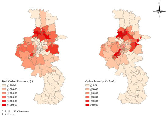
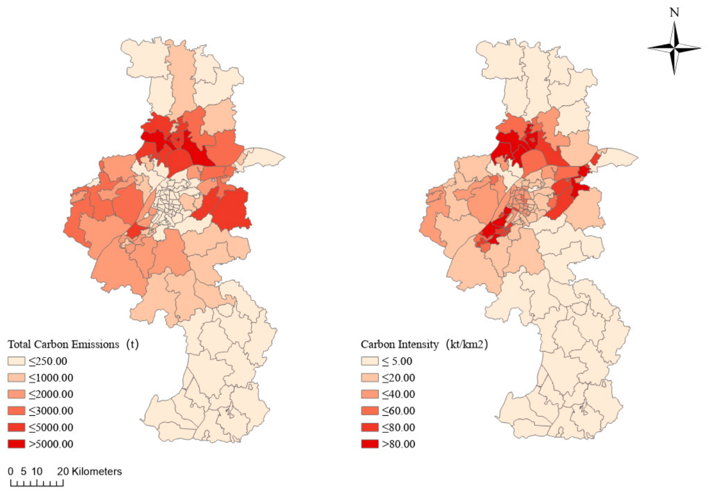
Based on Equation (4), the spatial distributions of total carbon emissions and carbon intensity in Nanjing are shown in Figure 4. The results indicate significant spatial heterogeneity in carbon emissions across the city, and clear differences can be observed between the spatial patterns of total emissions and carbon intensity. Areas with high carbon intensity are highly concentrated in the urban core, which is closely associated with intensive economic activities, commercial agglomeration, and high building density in these central districts.

Figure 4. Spatial patterns of total carbon emissions and carbon intensity in the study area.

According to the administrative statistics (Table 1), total building carbon emissions vary substantially among districts. This spatial heterogeneity is influenced not only by differences in physical area, but also by urban functional orientation and development stage. Specifically, Liuhe District ($\mathrm{37,112,153}$t), Qixia District ($\mathrm{21,552,888}$t), Pukou District ($\mathrm{18,819,783}$t), and Jiangning District ($\mathrm{14,815,173}$t) rank highest in total carbon emissions in Nanjing. These districts generally have large territorial areas and have served as major locations for industrial new towns and urban sub-centers during Nanjing’s spatial expansion. This development pattern, characterized by large-scale new area development, industrial clustering, and extensive infrastructure construction, has led to substantial building energy consumption and carbon emissions.

Table 1. Carbon emissions and carbon intensity by district in Nanjing.

District	Division Code	Area (km2)	Carbon Intensity (kt/km2)	CO2 Emissions (t)
Xuanwu District	320102	76.13	13.13	999,186.71
Qinhuai District	320104	49.17	17.26	848,702.27
Jianye District	320105	82.75	45.45	3,761,295.50
Gulou District	320106	53.01	26.39	1,399,270.82
Qixia District	320113	374	57.63	21,552,888.43
Yuhuatai District	320114	136.17	61.08	8,317,135.65
Jiangning District	320115	1579.85	9.38	14,815,173.03
Pukou District	320111	913.7	20.6	18,819,782.83
Liuhe District	320116	1481.66	25.05	37,112,152.63
Lishui District	320117	1062.76	1.64	1,747,112.17
Gaochun District	320118	797.51	0.98	779,799.85

In terms of carbon intensity, high values are mainly concentrated in the central urban area. Among all districts, Yuhuatai District has the highest carbon intensity, reaching $61.08 {\mathrm{kt}/\mathrm{km}}^2$, which is significantly higher than that of the other districts. Qixia District ($57.63 {\mathrm{kt}/\mathrm{km}}^2$) and Jianye District ($45.45 {\mathrm{kt}/\mathrm{km}}^2$) rank second and third, respectively, followed by Gulou District ($26.39 {\mathrm{kt}/\mathrm{km}}^2$). By contrast, Gaochun District ($0.98 {\mathrm{kt}/\mathrm{km}}^2$) and Lishui District ($1.64 {\mathrm{kt}/\mathrm{km}}^2$) show relatively low carbon intensity, which is consistent with the general pattern of urban development.

3.1.2. Statistical Characteristics of NTL Indices at Different Spatial Scales

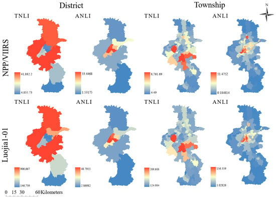
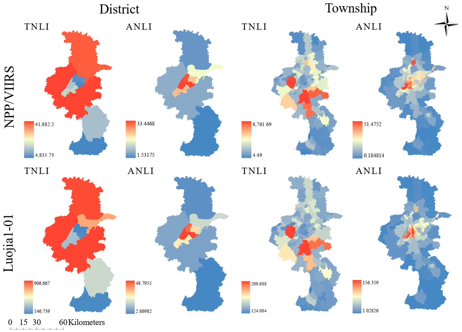
After data preprocessing, this study conducted spatial extraction and statistical analysis of two NTL remote sensing datasets, namely NPP/VIIRS and Luojia 1-01, at two core spatial scales: the district and subdistrict/township levels. To characterize nighttime light intensity in Nanjing more systematically, two indicators were derived, the Total Nighttime Light Index (TNLI) and the Average Nighttime Light Index (ANLI), which directly reflect total and relative brightness for each administrative unit and are well suited for carbon emission estimation using nighttime light imagery. The zonal statistical results of NPP/VIIRS and Luojia 1-01 at different spatial scales are shown in Figure 5.

Figure 5. TNLI and ANLI at district and township scales from two nighttime light datasets.

The results indicate that the two datasets exhibit a high degree of consistency in depicting the spatial distribution of nighttime light intensity. As the spatial scale was refined from the district level to the township level, the spatial heterogeneity captured by both datasets became more pronounced, although with slightly different emphases. In terms of ANLI, both data sources more clearly identified high-density areas, allowing the spatial pattern of human activity intensity to be represented in greater detail. In contrast, the distribution of TNLI at the township scale appeared more dispersed and was more strongly affected by differences in the area of administrative units, making it less suitable for independently reflecting the spatial pattern of activity density. This pattern was consistently observed in both the NPP/VIIRS and Luojia 1-01 results. Therefore, compared with TNLI, ANLI shows stronger spatial interpretability for analyzing the relationship between carbon emissions and NTL.

3.1.3. Relationship Between Carbon Emissions and NTL

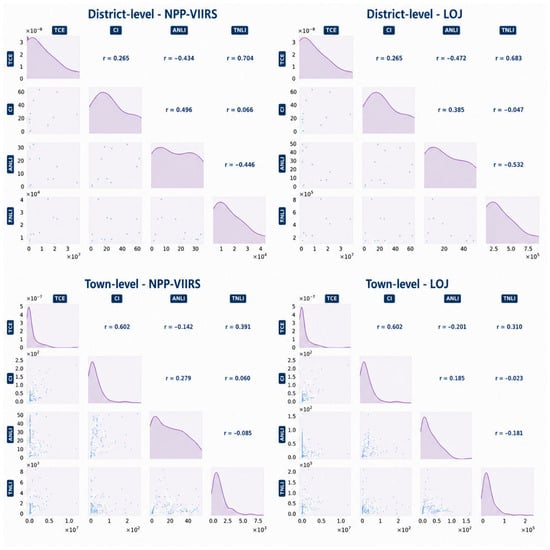
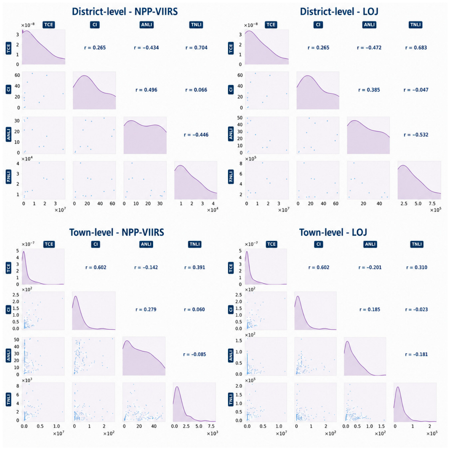
In this study, scatter plots and Pearson correlation analysis were used to examine the correspondence between carbon emission variables and NTL data, with the aim of identifying high-quality feature variables for subsequent estimation modeling. Variables with relatively weak correlations were excluded from the later modeling process. As shown in Figure 6, collinearity matrices were constructed to illustrate the relationships among variables at different spatial scales, including the district and community levels. In the matrix, the upper-right section presents the Pearson correlation coefficients between variables, the lower-left section shows the pairwise scatter plots, and the diagonal displays the probability density curves of individual variables.

Figure 6. Correlation matrix of carbon emissions and nighttime light indicators.

The correlation analysis shows that, at the district scale, TNLI derived from different NTL datasets is significantly positively correlated with total carbon emissions, with correlation coefficients of 0.704 and 0.683, respectively, both passing the significance test ($p<0.05$). This indicates that the total nighttime light intensity can effectively reflect the spatial pattern of carbon emissions at the district level. By contrast, ANLI is negatively correlated with TCE ($-0.434$ and $-0.472$) and shows a moderate positive correlation with carbon intensity ($0.496$ and $0.385$).

When the spatial scale is refined to the township level, TNLI and TCE, as well as ANLI and CI, still exhibit positive correlations. Moreover, the correlation patterns among variables become more stable, and the explanatory ability for total carbon emissions becomes more pronounced. Based on the above analytical results, this study adopts these two sets of variable combinations.

3.2. Comparison of Carbon Emission Estimation Models

3.2.1. Fitting Results of Non-Spatial Regression Models

The above correlation analysis reveals the associations between carbon emission indicators and NTL indices at different spatial scales. To construct estimation models linking carbon emissions and NTL, two variable pairs were selected from each dataset for regression analysis, namely TCE–TNLI and CI–ANLI at both the district and township scales.

Three commonly used functional forms, including linear, exponential, and logarithmic models, were employed to fit the relationship between carbon emissions and NTL. The corresponding $R^2$ values of different models are presented in Table 2.

Table 2. R-squared values of non-spatial regression models at different spatial scales.

Data Source	Spatial Scale	Variable	Linear Regression	Exponential Regression	Logarithmic Regression
NPP/VIIRS	District	TCE-TNLI	0.496	0.680	0.618
		CI-ANLI	0.246	0.383	0.366
	Township	TCE-TNLI	0.153	0.276	0.159
		CI-ANLI	0.078	0.305	0.118
LuoJia1-01	District	TCE-TNLI	0.466	0.615	0.597
		CI-ANLI	0.148	0.290	0.291
	Township	TCE-TNLI	0.096	0.220	0.122
		CI-ANLI	0.034	0.211	0.099

At the district level, the exponential regression model showed relatively better fitting performance for the TCE–TNLI variable combination, with $R^2$ values of 0.680 and 0.615 for NPP/VIIRS and Luojia 1-01, respectively, both of which were higher than those of the linear and logarithmic models. For the CI–ANLI combination, however, the overall fitting performance of both data sources was weak, with all regression models yielding $R^2<0.4$. This indicates that the linear and nonlinear relationships between carbon intensity and average nighttime light are relatively limited at the district scale.

When the spatial scale was further refined to the township level, the $R^2$ values of all variable combinations and regression models decreased significantly, indicating a clear decline in model performance. This finding suggests that, with increasing spatial refinement, the explanatory power of NTL indices for carbon emissions gradually weakens. In addition, the differences in $R^2$ between NPP/VIIRS and Luojia 1-01 were relatively small at the same spatial scale, indicating that the two data sources have comparable explanatory power for carbon emissions in Nanjing, and reveal that the two data sources have comparable explanatory power for carbon emissions, and spatial resolution discrepancies between the two datasets exert limited influence on the overall model accuracy across the study area.

3.2.2. Fitting Results of Spatial Regression Models and Tests of Spatial Dependence

To verify the necessity of introducing spatial regression into carbon emission estimation models, this study employed the global Moran’s $I$ statistic to test the spatial dependence of the dependent variables, namely total carbon emissions and carbon intensity. The results are presented in Table 3. In general, a positive Moran’s $I$ value with a $p$-value lower than 0.05 indicates that the observed variable exhibits a significant spatial clustering pattern.

Table 3. Global Moran’s I indices for spatial autocorrelation of carbon emission variables.

Spatial Scale	Variables	Moran’s I Index	z-Score	p-Value
District	TCE	0.256249	2.506319	0.0122
	CI	−0.017675	0.54091	0.588569
Township	TCE	0.58763	12.456788	0
	CI	0.384652	7.731877	0

The results reveal clear scale-dependent and variable-dependent differences in the spatial autocorrelation of carbon emissions in Nanjing. At the district scale, the Moran’s $I$ value of TCE is 0.256 ($p=0.012<0.05$), indicating a significant positive spatial correlation. In contrast, CI shows an approximately random spatial distribution at this scale. This may be attributed to the limitation of sample size. Additionally, total carbon emission data and carbon intensity data are greatly affected by regional land area.

When the spatial scale is refined to the township level, the spatial clustering characteristics of all dependent variables become much more pronounced. The Moran’s I values of TCE and CI increase sharply to 0.587 and 0.384, respectively, with both $p$-values approaching 0.000, indicating very strong positive spatial autocorrelation. Overall, at the same spatial scale, the spatial autocorrelation of TCE is consistently stronger than that of CI in Nanjing.

These findings suggest that, in terms of Nanjing, carbon emissions are not spatially independent. Therefore, when estimating carbon emissions from NTL imagery, especially at finer spatial scales, it is necessary to employ spatial regression models to reduce the errors caused by spatial autocorrelation.

Consistent with the non-spatial regression analysis, this study employed the SEM and SLM at both the district and township scales to examine the global relationships between carbon emissions and NTL while accounting for spatial autocorrelation. Considering that spatial autocorrelation at the district scale was not statistically significant, the GWR model was further introduced only at the township scale to explore local spatial characteristics at a finer level. The $R^2$ values of the spatial regression models for Nanjing are presented in Table 4.

Table 4. Model performance metrics of spatial regression models at different scales.

Data Sources	Spatial Scale	Variables	SEM (Pseudo R2)	SLM (Pseudo R2)	GWR (Global R2)
NPP/VIIRS	District	TCE-TNLI	0.645	0.758	——
		CI-ANLI	0.253	0.253	——
	Township	TCE-TNLI	0.525	0.527	0.577
		CI-ANLI	0.475	0.441	0.546
LuoJia1-01	District	TCE-TNLI	0.648	0.751	——
		CI-ANLI	0.155	0.164	——
	Township	TCE-TNLI	0.522	0.520	0.448
		CI-ANLI	0.448	0.433	0.555

The results show that, at the township scale, for the TCE–TNLI combination based on the NPP/VIIRS dataset, the GWR model achieved a global $R^2$ of 0.577, outperforming both the spatial error model ($R^2=0.525$) and the spatial lag model ($R^2=0.527$). This finding clearly demonstrates the superior capability of the GWR model in capturing spatial non-stationarity at the local scale.

Specifically, the exact optimal adaptive bandwidths derived from this verification process were 42 nearest neighbors for the NPP/VIIRS TCE–TNLI model, 29 nearest neighbors for the NPP/VIIRS CI–ANLI model, 37 nearest neighbors for the Luojia 1-01 TCE–TNLI model, and 32 nearest neighbors for the Luojia 1-01 CI–ANLI model.

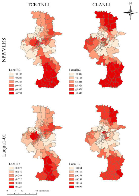
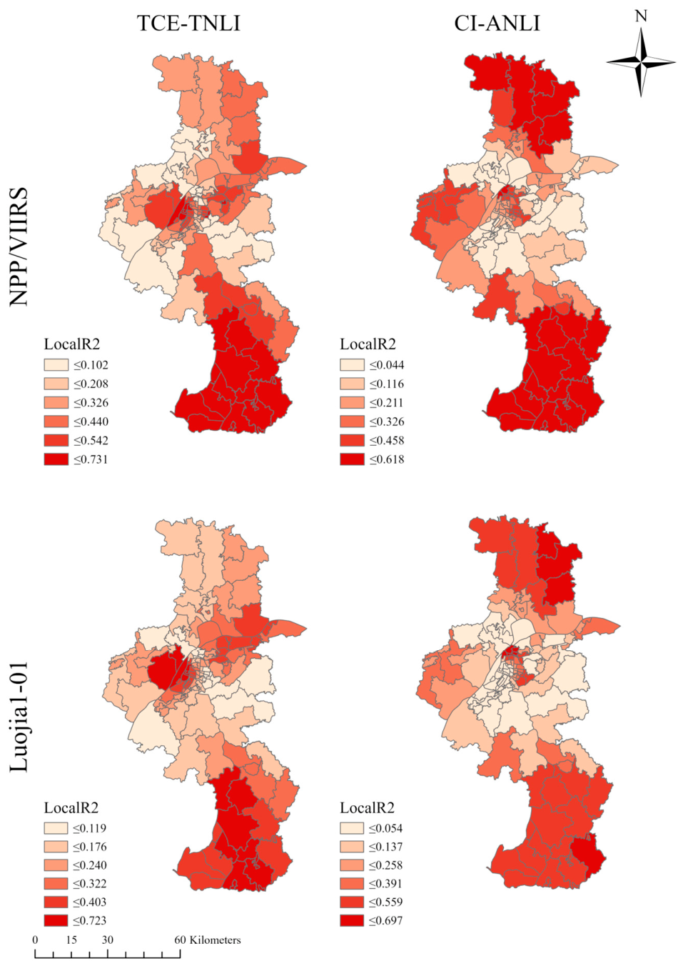
The spatial distribution of local $R^2$ values at the township scale derived from the GWR model is shown in Figure 7. For the TCE–TNLI variable pair, areas with the strongest association between total carbon emissions and NTL are consistently located in the southern and northern wings of Nanjing, including most townships in Gaochun District and Lishui District, as well as some townships in Liuhe District, together with several areas in the central–western part of the city, particularly in Pukou District. In these townships with high local $R^2$ values, the range calculated from NPP/VIIRS is 0.440–0.731, while the corresponding high-value range for Luojia 1-01 is 0.322–0.723. By contrast, areas with extremely low local $R^2$ values for the TCE–TNLI relationship are highly concentrated in the central urban core of Nanjing and the surrounding subdistricts, where local $R^2$ values are generally around 0.102.

Figure 7. Local R² of the GWR model at the township scale in Nanjing.

The spatial distribution of local $R^2$ values for the CI–ANLI variable pair shows considerable similarity to that of TCE–TNLI in the peripheral areas. High-fitting regions remain concentrated at the southern and northern edges of the city. Under the NPP/VIIRS dataset, the local $R^2$ values in these high-value areas range from 0.458 to 0.618, while under the Luojia 1-01 dataset, the corresponding range is 0.559–0.697. However, a marked divergence emerges in the urban core. Unlike the extremely low local $R^2$ values of TCE–TNLI in the central area, the CI–ANLI pair exhibits relatively strong spatial association in the central city and adjacent urban townships. According to the legend distribution, particularly under the Luojia 1-01 dataset, the local $R^2$ values of CI–ANLI in the urban core also reach the relatively high range of 0.559–0.697.

Overall, the spatial pattern suggests that the fitting performance of the TCE–TNLI combination shows strong spatial dependence in the peripheral townships of Nanjing, but remains weak in the highly urbanized central area. In contrast, the CI–ANLI combination not only maintains relatively high goodness of fit in peripheral areas, but also demonstrates strong spatial association in the urban core.

4. Discussion

4.1. Performance of Different Regression Models in Fitting the Relationship Between NTL and Carbon Emissions

By applying spatial regression models to the Nanjing dataset, the comparison between the two variable groups, TCE–TNLI and CI–ANLI, clearly demonstrates the applicability boundaries and statistical reliability of different models for estimating building carbon emissions [20]. According to the overall explanatory statistics of the GWR models shown in Table 5, the two variable combinations exhibit distinct fitting characteristics at the township scale. For the NPP/VIIRS dataset, the global $R^2$ of TCE–TNLI ($0.577$) is slightly higher than that of CI–ANLI ($0.546$). However, for the Luojia 1-01 dataset, the global $R^2$ of CI–ANLI ($0.555$) is markedly higher than that of TCE–TNLI ($0.448$). This result challenges the conventional assumption that total-value indicators necessarily outperform intensity-based indicators [23]. Consistent with the research conclusion of Shi et al. [20], total nighttime light indicators present better estimation performance in simulating urban carbon emissions compared with industrial carbon emissions, while the estimation accuracy of nighttime light proxies is obviously affected by urbanization development level and research spatial scale. Combined with the spatial distribution of local $R^2$, the results suggest that TCE–TNLI is more effective in capturing the expansion trend of total emissions in peripheral townships, whereas as the spatial scale becomes finer and urban density increases, CI–ANLI not only retains highly competitive overall explanatory power but also more sensitively reflects subtle variations within high-density urban areas, thereby effectively mitigating the scale effect caused by differences in the area of administrative units [22,56].

Table 5. Summary statistics of the GWR model at the township scale.

Data Sources	Spatial Scale	Variables	Global R2	Local R2 Range	Local R2 SD	AICc
NPP/VIIRS	Township	TCE-TNLI	0.577	0.033–0.731	0.188	4012.124
		CI-ANLI	0.546	0.005–0.618	0.198	1329.108
Luojia1–01	Township	TCE-TNLI	0.448	0.005–0.723	0.179	4021.749
		CI-ANLI	0.555	0.000–0.697	0.216	1323.713

To further evaluate the multidimensional performance of the GWR models, the standard deviation (SD) of local $R^2$ and the corrected Akaike information criterion were used to quantify [57,58,59], respectively, the spatial dispersion of the relationships and the parsimony of the models, as shown in Table 5. The results indicate that, under the same spatial scale, different variable combinations exhibit substantially different model characteristics. At the fine township scale, the GWR models perform effectively when validated against the authoritative EDGAR inventory baseline data, achieving robust global R² values approximate 0.55 that are competitive with the 0.50–0.60 range reported in recent micro-scale studies [30,31], while avoiding the artificially inflated correlations (R² > 0.8) common in macro-scale aggregations [21,28]. The CI–ANLI model demonstrates high parsimony and statistical robustness, with AICc values (approximately 1300) far lower than those of the TCE–TNLI model [46,60]. Meanwhile, its slightly higher local $R^2$ SD values (NPP/VIIRS: $0.198$; Luojia 1-01: $0.216$) objectively reflect the strong sensitivity of this intensity-based indicator to local spatial heterogeneity, especially across the urban core and urban–rural transition zones. In contrast, although the GWR model based on TCE–TNLI provides stronger explanatory performance in some areas, its substantially higher AICc values (exceeding 4000) suggest a potential risk of local overfitting when modeling extreme-value regions [61,62,63,64]. Overall, the CI–ANLI combination achieves a more balanced trade-off between predictive performance and model robustness in future applications.

A comparison of the fitting results from the two nighttime light remote sensing datasets further shows that, in the TCE–TNLI total-emission regression, the goodness-of-fit based on Luojia 1-01 imagery does decline to some extent [23,24]; however, this does not imply that high-resolution data are disadvantageous for spatial analysis. On the contrary, from the perspective of geospatial data processing, high-resolution imagery retains irreplaceable advantages. First, high-resolution data can effectively alleviate the blooming effect commonly found in conventional nighttime light imagery, as well as the pixel saturation problem in urban cores, thereby enabling more accurate delineation of the true physical boundaries of human activities. Second, consistent with the empirical observations of Cui et al. [24] and Wang et al. [26], the relatively lower accuracy of Luojia 1-01 in total-emission regression essentially stems from its strong sensitivity to subtle non-productive light sources within townships, such as micro-scale road networks and scattered lighting [51,64]. Although such fluctuations may be treated as noise in macro-scale total-emission regression, they actually indicate that high-resolution imagery contains much richer internal spatial structure than coarse-resolution pixels. This also explains why it can outperform lower-resolution data in CI–ANLI intensity-based regression. Therefore, for studies aiming to reveal complex intra-urban spatial heterogeneity, separate specific carbon emission sources, or further downscale the analysis to the grid level, high-resolution nighttime light data with greater fidelity and richer spatial detail remain the preferred foundation for high-quality spatial analysis and carbon estimation [65,66,67,68].

4.2. Prospects for Fine-Scale Carbon Emission Accounting

The multi-scale spatial regression framework adopted in this study provides a methodological reference for interpreting the spatial heterogeneity of urban carbon emissions. By integrating fine-resolution NTL datasets, this approach effectively captures the intensity and distribution of human activities at the township level, offering a viable path to bridge the gap between global-scale emission inventories and local-scale governance needs.

Rather than functioning as a direct operational policy deployment tool, the proposed framework is intended to serve as a scientific decision-support reference. It enables municipal authorities to identify emission hotspots and differentiate carbon governance strategies based on local urban functional characteristics [68,69]. The robustness of this spatial proxy-based method suggests its potential as a complementary tool in carbon accounting, particularly in regions where traditional bottom-up inventory data is sparse or temporally lagged [70,71,72]. Future applications could refine these models by incorporating multi-source socio-economic datasets to better align empirical findings with the complexity of urban energy transition pathways.

In discussing data source applicability, the relationship between spatial resolution and estimation accuracy is not simply linear [73,74]. At the township scale, high-resolution imagery provides abundant spatial detail but simultaneously amplifies background noise from non-productive light sources. Future research should focus on integrating multi-source spatial data—such as POI distributions and road networks—to reduce pixel-level noise, or applying super-resolution algorithms to extract higher-quality information from coarser imagery, thereby improving the robustness of fine-scale estimation [68,75].

Fine-scale carbon emission accounting holds important planning value, particularly for regions lacking detailed survey data. The analytical framework presented here offers a replicable and resource-efficient pathway for constructing preliminary urban carbon emission inventories using openly accessible remote sensing data. However, the models should be regarded as diagnostic tools for identifying spatial emission patterns rather than operationally validated instruments for direct policy deployment. Further multi-city validation is needed before these approaches can be more broadly applied in differentiated low-carbon governance.

4.3. Limitations

Several limitations of this study warrant acknowledgement. First, carbon emission data were spatially disaggregated from the gridded EDGAR_2025_GHG database rather than derived from direct field measurements, and the inherent uncertainties of this downscaling process may affect the reliability of township-level regression results [67]. Consistent with existing studies, refining carbon emissions to finer spatial scales tends to cause discrepancies in marginal areas [75,76,77]. At the 1 km scale, spatial distribution patterns can differ by 10–100%, with even more significant deviations of 90–100% in urban–rural transition zones [69,78]. Future work should incorporate bottom-up energy statistics or high-resolution activity data to strengthen inventory accuracy. Second, the use of a single-year NTL dataset (2018) precludes assessment of long-term temporal dynamics. Furthermore, although we utilized cloud-free composites and applied threshold corrections to filter out severe temporary anomalies like fires and flares, this study did not explicitly correct for residual atmospheric scattering or seasonal variability. These environmental factors introduce unavoidable observation biases. Consequently, the stability of the fitted models across years remains unverified, and future multi-temporal analyses incorporating rigorous atmospheric and seasonal calibrations are needed to confirm the framework’s temporal transferability [79,80,81]. Third, Luojia 1-01 imagery, despite its higher spatial resolution, is affected by noise from non-productive light sources and limited temporal availability, constraining its applicability to long-term or large-scale accounting; integration with auxiliary datasets such as POIs and land-use maps would help mitigate these effects [46,82]. Finally, as a single-city case study, the scale effects and model performance reported here may not generalize to cities with markedly different urban morphologies or economic structures, and cross-city validation remains an important direction for future research.

5. Conclusions

This study applies a multi-scale analytical framework to examine urban carbon emission estimation in Nanjing, combining NPP/VIIRS and Luojia 1-01 nighttime light imagery with non-spatial regression, spatial lag models, spatial error models, and geographically weighted regression. The main findings are as follows:

(1)

Carbon emissions in Nanjing exhibit pronounced spatial heterogeneity and clear scale effects. Total carbon emissions are concentrated in large outer districts, particularly Liuhe, Qixia, and Pukou, consistent with their roles as industrial new towns and urban sub-centres, whereas carbon intensity peaks in the urban core, reaching 61.08 kt/km² in Yuhuatai District. As the analytical scale is refined from district to township level, the spatial autocorrelation of both total carbon emissions (Moran’s I = 0.588) and carbon intensity (Moran’s I = 0.385) increases markedly, confirming that spatial regression models are essential at finer administrative scales.

(2)

At the township scale, GWR consistently outperforms global spatial models, underscoring the importance of capturing spatial non-stationarity in fine-scale carbon accounting. Of the two variable combinations examined, TCE–TNLI shows stronger explanatory power in peripheral and industrial townships, reflecting the spatial expansion of total emissions in outer districts. By contrast, CI–ANLI achieves more balanced performance across both peripheral and central urban areas, with substantially lower AICc values (approximately 1300 versus over 4000 for TCE–TNLI), indicating greater model parsimony and robustness. These results suggest that intensity-based indicators are better suited to fine-scale estimation in high-density urban environments.

(3)

The relationship between spatial resolution and estimation accuracy is not simply linear. Although Luojia 1-01 performs slightly below NPP/VIIRS in total-emission regression, attributable to its heightened sensitivity to non-productive light sources at the township scale, it achieves higher goodness-of-fit in the intensity-based CI–ANLI model (global R² = 0.555 versus 0.546). Its capacity to reduce pixel saturation in urban cores, delineate activity boundaries more precisely, and capture fine-grained intra-urban spatial structure makes it the preferable data source for detailed carbon estimation. Combining high-resolution NTL imagery with auxiliary datasets such as points of interest and road networks represents a promising avenue for further reducing estimation uncertainty.

(4)

By relying on open-access remote sensing and administrative data, the analytical approach adopted in this study offers a practical and replicable pathway for constructing fine-scale urban carbon emission inventories in data-scarce contexts. The comparative evaluation of model performance across scales and variable combinations provides methodological references for carbon accounting in other high-density cities, and the spatial evidence generated can inform differentiated low-carbon planning and targeted emission-reduction policy at the district and township levels.

Overall, these findings confirm that integrating fine-scale spatial econometrics with high-resolution nighttime light imagery offers a statistically reliable and practically replicable approach to precision urban carbon accounting and differentiated low-carbon governance.

References

- Xu, B.; Liu, Z.; Yan, S.; Schmitt, R.J.; He, X. Strategizing renewable energy transitions to preserve sediment transport integrity. Nat. Sustain. 2025, 8, 1314–1327. [Google Scholar] [CrossRef] [Scilit]
- Huang, Z.; Liu, Y.; Ma, H.; Luo, X.; Li, Z. Numerical investigation of exhaled droplet transmission and infection probability prediction in a subway compartment under ventilation and passenger effects with an improved Wells-Riley equation. Int. J. Heat Mass Transf. 2026, 265, 128809. [Google Scholar] [CrossRef] [Scilit]
- Lu, B.; Wang, W.; Jordan, N.; Wright, D.; Bechle, A.; Zoet, L.; Wu, C. A multi-scale assessment for managing coastal geomorphic changes in southwestern Lake Michigan. J. Environ. Manag. 2025, 395, 127878. [Google Scholar] [CrossRef] [Scilit] [PubMed]
- Münzel, T.; Sorensen, M. Heart healthy cities: Genetics loads the gun but the environment pulls the trigger. Eur. Heart J. 2021, 42, 2422–2438. [Google Scholar] [CrossRef] [Scilit]
- Elmqvist, T.; Andersson, E. Sustainability and resilience for transformation in the urban century. Nat. Sustain. 2019, 2, 267–273. [Google Scholar] [CrossRef] [Scilit]
- Wang, W.; Lu, B.; Li, Y.; Ji, F. Multiscale morphology-based detection of shoreline change hotspots from aerial imagery under fluctuating water levels. Remote Sens. 2026, 18, 1148. [Google Scholar] [CrossRef] [Scilit]
- He, S.; Wang, T.; Spicer, R.A.; Farnsworth, A.; Mulch, A.; Widdowson, M.; Zhang, Q.; Cai, F.; Valdes, P.J.; Wang, C.; et al. Back to an ice-free future: Early Cretaceous seasonal cycles of sea surface temperature and glacier ice. Sci. Adv. 2025, 11, eadr9417. [Google Scholar] [CrossRef] [Scilit]
- Shi, G.; Liu, J.; Yang, C.; An, Q.; Tian, Z.; Chen, C.; Zhang, J.; Li, X.; Zhang, Y.; Xu, J. Study on the spatiotemporal evolution of urban spatial structure in Nanjing’s main urban area: A coupling study of POI and nighttime light data. Front. Archit. Res. 2025, 15, 1–23. [Google Scholar] [CrossRef] [Scilit]
- Shi, K.; Xu, T. Effects of urban forms on CO2 emissions in China from a multi-perspective analysis. J. Environ. Manag. 2020, 262, 110300. [Google Scholar] [CrossRef] [Scilit]
- Shi, G.; Liu, J.; Na, J.; Chen, C.; Ma, H.; Feng, Z.; Sun, L. Patterns and synergistic effects of carbon emissions reduction from shared bicycles in the central urban district of Nanjing. Systems 2025, 13, 828. [Google Scholar] [CrossRef] [Scilit]
- Chen, G.; Shan, Y. Review on city-level carbon accounting. Environ. Sci. Technol. 2019, 53, 5545–5558. [Google Scholar] [CrossRef] [Scilit] [PubMed]
- Min, X.Z.; Zhang, X.; Xie, Z.Y.; Nikolaev, A.; Vorkamp, K.; Ma, J.M.; Reiersen, L.O.; Li, L.; Cai, M.H.; Ren, N.Q.; et al. Organic chemicals of Arctic concern in Russian coastal seas. Sci. Bull. 2025, 71, 946–959. [Google Scholar] [CrossRef] [Scilit]
- Wang, J.; Wei, J. High-resolution temporal and spatial evolution of carbon emissions from building operations in Beijing. J. Clean. Prod. 2022, 376, 134272. [Google Scholar] [CrossRef] [Scilit]
- Chen, P.; Nie, X.; Ning, Y.; Zhang, Y. Learning efficient and adaptive cross–channel dependencies for weakly-supervised object detection. IEEE Trans. Multimed. 2025, 27, 8954–8966. [Google Scholar] [CrossRef] [Scilit]
- Song, C.; Deng, Z. Developing urban building energy models for Shanghai city with multi-source open data. Sustain. Cities Soc. 2024, 106, 105425. [Google Scholar] [CrossRef] [Scilit]
- Li, Z.P. Toward low-carbon construction: A review of red mud utilization in cementitious materials and geopolymers for sustainability and cost benefits. Buildings 2026, 16, 362. [Google Scholar] [CrossRef] [Scilit]
- Cai, B.; Guo, H. Benchmarking carbon emissions efficiency in Chinese cities: A comparative study based on high-resolution gridded data. Appl. Energy 2019, 242, 994–1009. [Google Scholar] [CrossRef] [Scilit]
- Wei, W.; Zhang, X. Spatiotemporal dynamics of energy-related CO2 emissions in China based on nighttime imagery and land use data. Ecol. Indic. 2021, 131, 108132. [Google Scholar] [CrossRef] [Scilit]
- Liu, L.; Chu, C.; Chen, C.; Huang, S. MarineYOLO: Innovative deep learning method for small target detection in underwater environments. Alex. Eng. J. 2024, 104, 423–433. [Google Scholar] [CrossRef] [Scilit]
- Shi, K.; Chen, Z. NPP-VIIRS nighttime light data have different correlated relationships with fossil fuel combustion carbon emissions from different sectors. IEEE Geosci. Remote Sens. Lett. 2021, 18, 2062–2066. [Google Scholar] [CrossRef] [Scilit]
- Yang, D.; Luan, W. Modeling and spatio-temporal analysis of city-level carbon emissions based on nighttime light satellite imagery. Appl. Energy 2020, 268, 114696. [Google Scholar] [CrossRef] [Scilit]
- Chen, Z.; Yu, B. An extended time-series (2000–2018) of global NPP-VIIRS-like nighttime light data from a cross-sensor calibration. Earth Syst. Sci. Data 2021, 13, 889–906. [Google Scholar] [CrossRef] [Scilit]
- Ou, J.; Liu, X. Evaluation of Luojia 1-01 nighttime light imagery for impervious surface detection: A comparison with NPP-VIIRS nighttime light data. Int. J. Appl. Earth Obs. Geoinf. 2019, 81, 1–12. [Google Scholar] [CrossRef] [Scilit]
- Wang, Y.; Shen, Z. Comparing Luojia 1-01 and VIIRS nighttime light data in detecting urban spatial structure using a threshold-based kernel density estimation. Remote Sens. 2021, 13, 1574. [Google Scholar] [CrossRef] [Scilit]
- Yin, X.; Chen, L. Image object detection method based on improved faster R-CNN. J. Circuits Syst. Comput. 2024, 33, 2450130. [Google Scholar] [CrossRef] [Scilit]
- Wang, S.; Shi, C. Examining the spatial variations of determinants of energy-related CO2 emissions in China at the city level using geographically weighted regression model. Appl. Energy 2019, 235, 95–105. [Google Scholar] [CrossRef] [Scilit]
- Wang, W.; Dong, Q.; Hu, Z. Interactive piecewise planar building reconstruction from a single image based on geometric priors. Expert Syst. Appl. 2023, 230, 120572. [Google Scholar] [CrossRef] [Scilit]
- Ren, X.; Cheng, C. Spillover and dynamic effects of energy transition and economic growth on carbon dioxide emissions for the European Union: A dynamic spatial panel model. Sustain. Dev. 2021, 29, 228–242. [Google Scholar] [CrossRef] [Scilit]
- Xiang, C.; Mei, Y. Analysis of spatiotemporal changes in energy consumption carbon emissions at district and county levels based on nighttime light data—A case study of Jiangsu Province in China. Remote Sens. 2024, 16, 3514. [Google Scholar] [CrossRef] [Scilit]
- Li, R.; Yu, Y. Exploring the gradient impact of climate and economic geographical factors on city-level building carbon emissions in China: Characteristics and enlightenments. Sustain. Cities Soc. 2024, 113, 105637. [Google Scholar] [CrossRef] [Scilit]
- Fu, J.; Wang, C.; Liu, M.; Li, X.; Liu, Y.; Shi, W.; Wang, R. HyperR3SNet: Leveraging hyperbolic space and vision foundation models for remote sensing semantic segmentation. IEEE Trans. Geosci. Remote Sens. 2026, 64, 5620016. [Google Scholar] [CrossRef] [Scilit]
- Wang, M.; Wang, Y. Identifying the spatial heterogeneity in the effects of the construction land scale on carbon emissions: Case study of the Yangtze River Economic Belt, China. Environ. Res. 2022, 212, 113397. [Google Scholar] [CrossRef] [Scilit]
- Wang, L.; Ma, Y.; Yan, Z.; Zhang, L.; Hu, Y.; Zhao, S. Giving or receiving: Impact of online socializing in online fitness community on physical activity and emotional state. Comput. Hum. Behav. 2025, 169, 108669. [Google Scholar] [CrossRef] [Scilit]
- Cao, X.; Hu, Y. A simple self-adjusting model for correcting the blooming effects in DMSP-OLS nighttime light images. Remote Sens. Environ. 2019, 224, 401–411. [Google Scholar] [CrossRef] [Scilit]
- Wang, Z.; Zhou, H.; Liu, H. Physics-informed neural networks based digital volume correlation for displacement and strain measurements. Mech. Syst. Signal Process. 2026, 248, 113998. [Google Scholar] [CrossRef] [Scilit]
- Cheon, S.; Kim, J.-A. Quantifying the influence of urban sources on night light emissions. Landsc. Urban Plan. 2020, 204, 103936. [Google Scholar] [CrossRef] [Scilit]
- Liu, S.; Zhang, J.; Lin, Z.; Wang, J. Assessment of rockburst proneness in thermally-damaged fractured granite: A quantitative analysis of energy evolution and strain localization intensity. Theor. Appl. Fract. Mech. 2026, 145, 105677. [Google Scholar] [CrossRef] [Scilit]
- Chuai, X.; Yuan, Y. Multiangle land use-linked carbon balance examination in Nanjing City, China. Land Use Policy 2019, 84, 305–315. [Google Scholar] [CrossRef] [Scilit]
- Liu, Y.; Huang, Z.; Luo, X.; Ma, H.; Li, Z. Insights of airborne transmission within urban rail transit carriage environments after the COVID-19 pandemic. Indoor Built Environ. 2026. [Google Scholar] [CrossRef] [Scilit]
- Wang, J.; Huang, Y. Can buildings sector achieve the carbon mitigation ambitious goal: Case study for a low-carbon demonstration city in China? Environ. Impact Assess. Rev. 2021, 90, 106633. [Google Scholar] [CrossRef] [Scilit]
- Zhang, D.; Shan, C.; Li, F.; Liu, P.; Xing, Y.; Lan, X.; Cao, G.; Liu, L.; Liu, Y.; Leng, J. Preliminary design and validation of a hybrid triangular rollable and collapsible boom based on high strain and shape memory polymer composites. Compos. Part B Eng. 2026, 318, 113647. [Google Scholar] [CrossRef] [Scilit]
- Liu, X.; Li, X. Luojia nighttime light data with a 130 m spatial resolution providing a better measurement of gridded anthropogenic heat flux than VIIRS. Sustain. Cities Soc. 2023, 94, 104565. [Google Scholar] [CrossRef] [Scilit]
- Levin, N.; Kyba, C.C.M. Remote sensing of night lights: A review and an outlook for the future. Remote Sens. Environ. 2020, 237, 111443. [Google Scholar] [CrossRef] [Scilit]
- Lv, J.; Wang, C.; Xie, L. Lyapunov-like characterization of stipulated-time stability: Controller and observer design. IEEE Trans. Syst. Man Cybern. Syst. 2025, 55, 4877–4889. [Google Scholar] [CrossRef] [Scilit]
- Lin, J.; Shi, W. Improved denoising of VIIRS nighttime light imagery for estimating electric power consumption. IEEE Geosci. Remote Sens. Lett. 2019, 17, 1782–1786. [Google Scholar] [CrossRef] [Scilit]
- Gan, L.; Liu, Y. Regional inequality in the carbon emission intensity of public buildings in China. Build. Environ. 2022, 225, 109657. [Google Scholar] [CrossRef] [Scilit]
- Li, P.R.; Zhang, H.R. A spatial finer electric load estimation method based on night-light satellite image. Energy 2020, 209, 118475. [Google Scholar] [CrossRef] [Scilit]
- Wu, Y.; Jiang, M. Does China’s urban development satisfy Zipf’s law? A multiscale perspective from the NPP-VIIRS nighttime light data. Int. J. Environ. Res. Public Health 2020, 17, 1460. [Google Scholar] [CrossRef] [Scilit] [PubMed]
- Ai, M.S.; Chen, X. Spatial correlation analysis between human disturbance intensity (HDI) and ecosystem services value (ESV) in the Chengdu-Chongqing urban agglomeration. Ecol. Indic. 2024, 158, 111555. [Google Scholar] [CrossRef] [Scilit]
- Lv, J.; Wang, C.; Xie, L. Distributed output-feedback leader-following consensus of nonlinear multiagent systems. Automatica 2025, 177, 112281. [Google Scholar] [CrossRef] [Scilit]
- Teng, S.N.; Xu, C. Effects of intrinsic sources of spatial autocorrelation on spatial regression modelling. Methods Ecol. Evol. 2018, 9, 363–372. [Google Scholar] [CrossRef] [Scilit]
- Wang, Y.N.; Li, S.K.; Li, Z.Y.; Garg, A. Exploring the application of the MICP technique for the suppression of erosion in granite residual soil in Shantou using a rainfall erosion simulator. Acta Geotech. 2023, 18, 3273–3285. [Google Scholar] [CrossRef] [Scilit]
- Mollalo, A.; Vahedi, B. GIS-based spatial modeling of COVID-19 incidence rate in the continental United States. Sci. Total Environ. 2020, 728, 138884. [Google Scholar] [CrossRef] [Scilit]
- Elhorst, J.P. Applied spatial econometrics: Raising the bar. Spat. Econ. Anal. 2010, 5, 9–28. [Google Scholar] [CrossRef] [Scilit]
- Du, Z.; Wang, Z. Geographically neural network weighted regression for the accurate estimation of spatial non-stationarity. Int. J. Geogr. Inf. Sci. 2020, 34, 1353–1377. [Google Scholar] [CrossRef] [Scilit]
- Pani, A.; Sahu, P.K. Assessing the extent of modifiable areal unit problem in modelling freight (trip) generation: Relationship between zone design and model estimation results. J. Transp. Geogr. 2019, 80, 102524. [Google Scholar] [CrossRef] [Scilit]
- Li, Y.; Zhou, B. Context sensitivity of surface urban heat island at the local and regional scales. Sustain. Cities Soc. 2021, 74, 103146. [Google Scholar] [CrossRef] [Scilit]
- Liu, S.; Zhao, C.; Lin, Y.; Wen, Z. Microstructure-engineered shear thickening composites with controllable switching of rigid/flexible impact modes for adaptive protection. Compos. Part A Appl. Sci. Manuf. 2026, 206, 109750. [Google Scholar] [CrossRef] [Scilit]
- Liu, S.; Zhang, Z.; Wu, Q.; Feng, C.; Chen, C.; Hu, X. Cross-scale crack evolution in pre-flawed sandstone under high temperature: Insights from a composition-aware thermal-mechanical grain-based model. Theor. Appl. Fract. Mech. 2026, 143, 105450. [Google Scholar] [CrossRef] [Scilit]
- Wu, Q.; Zhang, Y.; Wang, X.; Sun, Y.; Li, Y.; Zhu, G. Crystallization of hard spheres within ellipsoidal confinement. Phys. Rev. E 2026, 113, 025422. [Google Scholar] [CrossRef] [Scilit] [PubMed]
- Zhang, Y.; Teoh, B.K. Exploring driving force factors of building energy use and GHG emission using a spatio-temporal regression method. Energy 2023, 269, 126747. [Google Scholar] [CrossRef] [Scilit]
- Zhang, M.S.; Chiu, C.F.; Wang, Y.N. Analysis of microbial methane oxidation capacity of landfill soil cover using quorum sensing. Environ. Res. 2025, 268, 120781. [Google Scholar] [CrossRef] [Scilit]
- Li, Y.; Qu, K.; Jiang, R.; Wang, H.; Zhao, X.; Yang, Z.; Tian, B.; Tao, J.; Chu, J.; Duan, C. Atomic-scale defect reconfiguration via thermally induced structural ordering for high-efficiency Sb2Se3 solar cells. ACS Nano 2025, 19, 33460–33472. [Google Scholar] [CrossRef] [Scilit]
- Gu, Y.; Zhu, L.; Li, J.H.; Zhao, G.Y. Preview MPC control of train active suspension based on Kalman filter disturbance estimation. Measurement 2026, 268, 120616. [Google Scholar] [CrossRef] [Scilit]
- Xu, B.; Zheng, Y.; Li, W.; Gao, X.; Gong, D.; He, J.; Fan, Z. Handling multiobjective optimization problems with complex constraints: A constraints grouping-based approach. IEEE Trans. Syst. Man Cybern. Syst. 2025, 55, 3866–3880. [Google Scholar] [CrossRef] [Scilit]
- Zuo, T.Y.; Di, K.; Li, P.; Jiang, Y. Autonomous domain adaptation self-optimization approach for cross-domain industrial agents. ACM Trans. Intell. Syst. Technol. 2026, 17, 1–25. [Google Scholar] [CrossRef] [Scilit]
- Yang, J.; Deng, Z. Development of bottom-up model to estimate dynamic carbon emission for city-scale buildings. Appl. Energy 2023, 331, 120410. [Google Scholar] [CrossRef] [Scilit]
- Zhang, M.; Yang, Z.; Ma, Y.; Huang, T.; Li, Q.; Gong, P.; Deng, L.; Jin, J.; Liu, J.; Guo, P.; et al. Oxide growth and surface fracture during high-temperature oxidation of Zr55Cu30Al10Ni5 metallic glass powders. Appl. Surf. Sci. 2026, 736, 166816. [Google Scholar] [CrossRef] [Scilit]
- Gao, Y.; Wang, Y.; Yang, N.; Wang, Q.; Javadi, B.; Ai, Q.; Zhu, J. Multi-timescale distributed control for multi-energy virtual power plant clusters via cloud-edge collaboration. Appl. Energy 2026, 414, 127835. [Google Scholar] [CrossRef] [Scilit]
- Li, K.; Bao, X.; Li, G.; Wang, Y.; Zhu, B.; Cao, Z. Design and fundamental dynamic mechanical analysis of large-scale submerged buoy systems: Experiment and numerical simulation. Ocean Eng. 2026, 357, 125515. [Google Scholar] [CrossRef] [Scilit]
- Zhang, L.; Wu, T. Solving SAT by restricted spiking neural P systems with temporal division rules. Theor. Comput. Sci. 2026, 1078, 116009. [Google Scholar] [CrossRef] [Scilit]
- Oda, T.; Bun, R.; Kinakh, V. Errors and uncertainties in a gridded carbon dioxide emissions inventory. Mitig. Adapt. Strateg. Glob. Change 2019, 24, 1007–1050. [Google Scholar] [CrossRef] [Scilit]
- Li, Y.; Zhang, X.; He, Z.; Xie, J.; Zhang, Y.; Wang, J.; Deng, J. Response of sludge EPS under the action of coupled alternating electric field-ammonium persulfate dewatering technology: Structural changes and mechanism analysis. Chem. Eng. Sci. 2025, 323, 123267. [Google Scholar] [CrossRef] [Scilit]
- Qi, H.X.; Yang, S.Y.; Miao, Y.H.; Cui, L.G.; Xue, H.; Hua, J.D.; Hong, K.; Fang, Y.Y. Prediction of sperm retrieval outcomes based on testicular ultrasound images and dense convolutional sparse coding. IEEE Sens. J. 2026, 26, 7292–7307. [Google Scholar] [CrossRef] [Scilit]
- Tong, T.; Qu, W.; Hua, J.; Chen, D.; Tan, J.; Lin, J. Delamination detection in composite laminates using Lamb wave tomographic method based on sparse and probabilistic reconstruction. NDT E Int. 2026, 160, 103650. [Google Scholar] [CrossRef] [Scilit]
- Li, B.R.; Liu, C.L.; Liu, P.J.; Zhou, T.L.; Xu, W.J.; Wang, L.Q.; Ye, L. Predictive Analysis of the Overall Cooling Effectiveness for Leading-Edge Showerhead Cooling Based on a Thermal Resistance Network Model with Physical Corrections. Aerosp. Sci. Technol. 2026, 176, 112492. [Google Scholar] [CrossRef] [Scilit]
- Ye, L.; Li, Z.H.; Yan, H.N.; Liu, C.; Cho, H.H.; Guo, T. Predicting Film-Cooling Effectiveness of Compound-Angle Holes Using a POD-Based Hybrid Deep Learning Model. Aerosp. Sci. Technol. 2026, 176, 112590. [Google Scholar] [CrossRef] [Scilit]
- Liu, D.; Lian, J.; Liu, F.; Ma, B.; Liu, D.; Shi, J.; Gou, W.; Li, H.; Zheng, Y.; Xu, C.; et al. A refined numerical model for assessing low-pressure effects on ski-jump atomization at high-altitude dams. J. Mt. Sci. 2026, 1–24. [Google Scholar] [CrossRef] [Scilit]
- Yang, T.; Qian, Z.; Hang, N.; Liu, M. S-PINN: Stabilized physics-informed neural networks for alleviating barriers between multi-level co-optimization. Comput. Methods Appl. Mech. Eng. 2025, 447, 118348. [Google Scholar] [CrossRef] [Scilit]
- Yang, H.; Liu, J.; Mu, W. A novel crack depth quantification index based on acoustic emission modeling of thin plate cracks. Measurement 2026, 270, 120888. [Google Scholar] [CrossRef] [Scilit]
- Weng, Y.; Yang, K.; Liu, Z.; He, W.; Tang, X. Lgvlm-miot: A lightweight generative visual-language model for multilingual IOT applications. IEEE Internet Things J. 2025, 12, 13311–13326. [Google Scholar] [CrossRef] [Scilit]
- Liu, X.; Wang, C.; Chen, C.; Pan, Z.; Gao, C.; Lai, W.; Zhao, J.; Tian, T.; Xiao, W. Recent advances in hierarchical porous materials for CO2 capture and utilization. Coord. Chem. Rev. 2025, 544, 216927. [Google Scholar] [CrossRef] [Scilit]
Disclaimer/Publisher’s Note: The statements, opinions and data contained in all publications are solely those of the individual author(s) and contributor(s) and not of MDPI and/or the editor(s). MDPI and/or the editor(s) disclaim responsibility for any injury to people or property resulting from any ideas, methods, instructions or products referred to in the content. |
© 2026 by the authors. Licensee MDPI, Basel, Switzerland. This article is an open access article distributed under the terms and conditions of the Creative Commons Attribution (CC BY) license.