Research on Intelligent Fault Diagnosis of Reciprocating Compressor Valves Based on Multi-Source Information Fusion with Improved SWD

Abstract

Aiming at solving the problems of the complex impact vibration characteristics of reciprocating compressor valves, the inability of a single signal to fully characterize state characteristics, and the difficulty of effectively extracting and fusing feature information from multi-source signals, this paper constructs a fault diagnosis and prediction model combining Improved Swarm Decomposition (ISWD) and t-SNE dimensionality reduction and fusion with a Multi-scale Convolutional Neural Network–Bidirectional Gated Recurrent Unit (MCNN-BiGRU) based on multi-source signals and applies it to the fault diagnosis and pattern recognition prediction of reciprocating compressor valves. Firstly, atom search optimization (ASO) is adopted to optimize the decomposition parameters of Swarm Decomposition (SWD) to obtain the ISWD algorithm, which is applied to decompose the multi-source signals of compressors to extract the oscillating components (OCs). Secondly, the correlation coefficient method is used to screen the OCs and conduct signal reconstruction, and various entropy feature values are extracted from the reconstructed signals to form an initial feature set. Then the t-SNE algorithm is employed to perform dimensionality reduction and fusion on the initial feature set, yielding a more concise and representative fused feature set. Finally, the fused feature set after dimensionality reduction and fusion is input into the MCNN-BiGRU model for training, so as to realize the pattern recognition and prediction of valve faults. The effectiveness and superiority of this method in the fault diagnosis of reciprocating compressor valves are verified through numerical simulation and experimental analysis.

1. Introduction

Reciprocating compressors are widely applied in key industrial fields such as the petrochemical industry and mining industry due to their high compression efficiency and broad applicability. As the core power components of reciprocating compressors, the operating status of valves directly determines the reliability of the unit and the continuity of production. Once a fault occurs, it is prone to causing problems such as a sharp increase in noise, gas leakage and component wear, which will eventually lead to production interruption and economic losses [1]. Therefore, it is crucial to carry out accurate fault detection and diagnosis on valves. The industrial demand for the fault-free operation of equipment has driven the development of mechanical condition monitoring technology, forming technical approaches including vibration analysis, oil analysis and acoustic emission detection [2]. Vibration signals can reflect the macroscopic mechanical impact abnormalities of valves, while acoustic emission signals are capable of capturing the evolution of microscopic defects. These two types of signals provide complementary information for fault diagnosis [3]. Fault diagnosis based on a single vibration signal is liable to result in missed judgments and misjudgments due to one-sided information, whereas multi-source signal fusion can fully characterize the fault state from dual dimensions and has thus become a mainstream research direction. However, multi-source signals induced by valve faults exhibit strong non-stationary and nonlinear characteristics and are subject to background noise interference. It is difficult to extract features accurately with traditional signal processing methods (e.g., Fourier transform). Benefiting from superior adaptability, non-stationary signal processing methods based on advanced decomposition theories have become core solutions to this issue and have gained widespread attention [4].

For non-stationary signals, wavelet transform is a typical time–frequency analysis method. It decomposes signals into different frequency bands to extract fault features [5]. However, its wavelet basis functions and decomposition parameters are determined empirically, leading to poor adaptability to the vibration–acoustic emission multi-source heterogeneous signals of reciprocating compressor valves and easy loss of key fault information. Huang et al. [6] proposed the Empirical Mode Decomposition (EMD) algorithm, which can adaptively decompose signals with composite components into several single components; however, it has the defects of poor noise resistance and mode mixing, and easily confuses the low-frequency impact components of vibration with the high-frequency stress-wave components of acoustic emission when processing multi-source signals. To overcome this drawback, several improved methods (EEMD [7], CEEMD [8], MEEMD [9]) have been proposed based on EMD, which are further refined to develop the CEEMDAN algorithm [10]. Bie et al. [7] proposed an improved Complete Ensemble Empirical Mode Decomposition with Adaptive Noise (ICEEMDAN) algorithm addressing the challenge of fault feature extraction in reciprocating machinery, which improved the efficiency of the algorithm. However, these algorithms generally suffer from high computational complexity and significant end effects, which greatly increase the computational cost in multi-source signal processing and hinder the accurate separation of different modal signals [11]. Dragomiretskiy et al. [12] proposed the Variational Mode Decomposition (VMD) algorithm. By setting an appropriate decomposition number K and penalty factor α, this algorithm exhibits strong robustness toward noisy non-stationary signals. However, the parameters K and α directly affect the decomposition results, and their selection relies on human experience. Therefore, Lu et al. [13] introduced the Whale Optimization Algorithm (WOA) to optimize the VMD algorithm, which can automatically determine the optimal parameter combination of VMD. The superiority of this method was verified in rotor fault diagnosis, but it does not perform well for the multi-source heterogeneous signals of compressor valves. The aforementioned traditional decomposition algorithms struggle to meet the precise decomposition requirements of multi-source heterogeneous signals from reciprocating compressor valves, mainly due to empirical parameter dependence, severe mode mixing, and excessively high computational cost.

In contrast, the Swarm Decomposition (SWD) algorithm based on the Synchrosqueezing Wavelet Filter (SWF) model proposed by Georgios et al. [14] can iteratively extract oscillatory components (OCs) from multi-component signals. Wang et al. [15] applied it to non-stationary signal processing of gearboxes and confirmed that the adaptability and decomposition accuracy of this algorithm are superior to traditional methods. Nevertheless, the original SWD still suffers from parameter dependence issues: improper threshold setting tends to cause over-decomposition or under-decomposition, and the generated false frequency components will interfere with the extraction of fault features from multi-source signals [16].

To solve this problem, the Atomic Search Optimization (ASO) algorithm is employed to optimize the SWD parameters, and the Improved Swarm Decomposition (ISWD) algorithm is established. This algorithm can adaptively search for the optimal threshold matching the characteristics of the multi-source signals, freeing the model from manual parameter tuning and reducing reliance on empirical experience in traditional algorithms. Its iterative filtering mechanism can accurately distinguish the low-frequency impact features of vibration signals from the high-frequency defect features of acoustic emission signals, avoiding the mode mixing problem of EMD-series algorithms. Moreover, it has lower computational complexity than ensemble decomposition algorithms. High processing efficiency can be achieved without compromising decomposition accuracy. Benefiting from satisfactory noise immunity, fault-related characteristic components can be well preserved under intense industrial noise.

After obtaining the optimal components through ISWD, the correlation coefficient method is used to screen the reconstructed signals. These reconstructed signals carry sufficient valve condition information but also involve plenty of invalid and redundant components. Traditional time-domain features struggle to characterize signal nonlinearity, while frequency-domain features are susceptible to operating conditions and lose transient information [17]. As a metric for measuring time-series complexity and nonlinearity, entropy is effective for fault feature description, while a single entropy index shows limited representation ability [18]. Therefore, this paper extracts multiple complementary information entropies to construct an initial feature set and eliminates noise and redundancy through multi-entropy fusion to improve the distinguishability of fault features, laying a foundation for subsequent pattern recognition.

The MCNN-BiGRU model integrates the local feature enhancement capability of the Multi-scale Convolutional Neural Network (MCNN) and the advantages of the Bidirectional Gated Recurrent Unit (BiGRU) concerning the modeling of temporal dependence. [19] It possesses excellent nonlinear mapping ability, temporal feature capture capability, and high fault tolerance [20]. Moreover, it is highly compatible with the output features of the Improved Synchrosqueezing Wavelet Decomposition (ISWD) algorithm. After the multi-source vibration and acoustic emission signals of the compressor valves are decomposed and reconstructed via ISWD, the extracted entropy features can reflect the local impulse characteristics induced by valve faults as well as the implicit temporal evolution rules of faults [21]. The multi-scale convolutional kernels adopted in MCNN can enhance the discrimination ability of local fault features. BiGRU is capable of mining temporal dependencies within feature sequences. Such characteristics strongly match the inherent properties of features decomposed by ISWD, thereby achieving in-depth analysis of fault characteristics [22].

Comparing this with traditional neural networks and other classifiers including SVM, SVM suffers from weak generalization capability faced with high-dimensional temporal fused features and fails to fit complex nonlinear distributions of multi-source features. Traditional neural networks lack the ability to model temporal features and cannot capture the evolution law of valve faults with operating cycles or the integrity of multi-source signals. For this reason, the processed features are fed into the MCNN-BiGRU model rather than conventional classifiers like SVM to realize valve fault pattern recognition.

Based on the above discussion, this study proposes a novel model combining improved SWD and MCNN-BiGRU for the fault diagnosis of reciprocating compressor valves from the feature fusion perspective. Firstly, the Atomic Search Optimization (ASO) algorithm is adopted to optimize the threshold parameters of SWD for multi-source signal decomposition, to enhance both decomposition accuracy and computational efficiency. Secondly, the reconstructed oscillatory components are screened by the correlation coefficient method for denoising, and multiple types of information entropy features are extracted. Then, a fused feature set is constructed through t-SNE dimensionality reduction and fusion. Finally, the feature set is fed into the MCNN-BiGRU model for training to achieve accurate recognition of valve fault patterns. The diagnostic performance and effectiveness of the proposed method are verified by numerical simulation and experimental results.

The main innovations and contributions of this work are summarized as follows:

(1)

Aiming at resolving issues arising from the non-stationary and coupled characteristics of reciprocating compressor vibration and acoustic emission signals, an Improved Swarm Decomposition (ISWD) algorithm optimized by atom search optimization (ASO) is proposed to achieve adaptive, high-precision signal decomposition. This method overcomes the low accuracy and poor adaptability caused by manual parameter selection in traditional decomposition methods.

(2)

A t-SNE-based nonlinear dimensionality reduction and fusion strategy is constructed for high-dimensional entropy features extracted from vibration and acoustic emission signals. It makes full use of multi-source information complementarity, enhances fault sample separability, reduces redundant information, and provides high-quality low-dimensional feature input for subsequent classification modeling.

(3)

A hybrid MCNN-BiGRU model is designed to simultaneously capture the multi-scale spatial features and bidirectional temporal dependencies of multi-source signals. The complete end-to-end fault diagnosis framework is verified on a real reciprocating compressor test bench, which significantly improves diagnostic accuracy, robustness and engineering practicability.

The structure of this paper is as follows: Section 2 describes the principles of ISWD, feature fusion, and MCNN-BiGRU and introduces the framework of the diagnosis model. In Section 3, the feasibility of the ISWD method for fault diagnosis of reciprocating compressor valves is verified by numerical simulation. Section 4 introduces the fault simulation experiment with reciprocating compressor valves and carries out experimental verification. Section 5 is used to summarize the paper.

2. Algorithm Theory

2.1. ISWD Algorithm

The SWD algorithm [17] is an intelligent decomposition algorithm that implements a cyclic iterative group filtering operation using mathematical principles. Based on the SWF, the SWD algorithm establishes a group model, wherein the input signal is treated as a predation path and a group hunting process is simulated to output values derived from this path. In the group model, the input discrete time-domain signal $x\left[n\right]$ is regarded as the prey, as shown in the following equation.

$$P_{prey}\left[n\right]=x_i\left[n\right],n=1,2,3\dots ,L$$

(1)

In the equation, $p_{prey}\left[n\right]$ is defined as the position of the prey at the n-th step. Each swarm is composed of M individuals, and $x_i\left[n\right]$ is regarded as the signal of the i-th individual at each time step n, whose state information is represented by position $p_i\left[n\right]$ and velocity $v_i\left[n\right]$, respectively.

The movement and hunting behaviors of the group individuals are governed by two types of forces to accomplish the hunting process. The first is the driving force, which is generated by self-drive; the second is the cohesive force, derived from the mutual attraction or repulsion among group individuals. When group individuals attract each other, they share a consistent search target, whereas repulsion can avoid collisions among members and improve search efficiency. The two forces are defined by the following equations.

$$\left\{\begin{array}{l}{F}_{dr,i}^n=P_{prey}\left[n\right]-p_i\left[n-1\right]\\ F_{coh,i}^n={\displaystyle \frac{1}{M-1}}·{\displaystyle \sum _{j=1,j\ne 1}^{M}f\left(p_i\left[n-1\right]-p_j\left[n-1\right]\right)}\\ f\left(d\right)=-\mathrm{sgn}\left(d\right)·\ln \left({\displaystyle \frac{⌊d⌋}{d_{cr}}}\right)\end{array}\right.$$

(2)

where $F_{dr,i}^n$ denotes the driving force acting on the i-th individual at time step n; $F_{coh,i}^n$ denotes the cohesive force acting on the i-th individual at time step n; $f\left(d\right)$ determines the allocation between the attractive and repulsive forces exerted by the j-th individual on the i-th individual at distance d; sgn(·) is the sign function; and $d_{cr}$ represents the critical distance below which two individuals do not interact when $f\left(d_{cr}\right)=0$, whose magnitude is equal to the root mean square (RMS) value of the input signal.

To track the prey, the position and velocity of group individuals are adjusted so that their states can be updated. The update equations are given as follows.

$$\left\{\begin{array}{l}{p}_i\left[n\right]=p_i\left[n-1\right]+\delta ·v_i\left[n\right]\\ v_i\left[n\right]=v_i\left[n-1\right]+\delta ·\left(F_{dr,i}^n\left[n\right]+F_{coh,i}^n\left[n\right]\right)\end{array}\right.$$

(3)

In the formula, $p_i\left[n\right]$ is defined as the position; $v_i\left[n\right]$ is regarded as the velocity; $\delta$ is adopted as the time interval between two consecutive time steps, by which the flexibility of the group is controlled.

The signal $y\left[n\right]$, namely the trajectory of the group, is iteratively output by the SWF, as expressed in the following equation.

$$y\left[n\right]=\beta ·{\displaystyle \sum _{i=1}^M{p}_i\left[n\right]}$$

(4)

In the formula, β is adopted as the scaling factor, which is generally set to 0.005 [20]. The group behavior is governed by the parameters $\delta$ and M of the SWF. By iterative application of the SWF with these two parameters, the final form of the oscillatory components is obtained, as calculated in the following equation.

$$\left\{\begin{array}{l}M\left(\overline{\omega }\right)=33.46{\overline{\omega }}^{-0.735}-29.1\\ \delta \left(\overline{\omega }\right)=-1.5{\overline{\omega }}^{-2}+3.454\overline{\omega }-0.001\end{array}\right.$$

(5)

In the formula, $\overline{\omega }$ is defined as the normalized frequency.

The latest oscillatory components are obtained via continuous iterative operations of the SWF, and the iteration terminates when the remaining input signal contains no significant information. In the theoretical calculation, the component corresponding to the maximum amplitude in the energy spectrum is selected as the candidate new mode for extraction in each iteration. The iteration terminates when the variance of output signals from two consecutive iterations is below the predefined threshold StD.

$$StD={\displaystyle \sum \frac{{\left|y_i\left[n\right]-y_{i-1}\left[n\right]\right|}^2}{y_{i-1}{\left[n\right]}^2}}$$

(6)

To improve the search efficiency, a Savitzky–Golay (SG) filter is adopted to smooth the energy spectrum. Meanwhile, to reduce the search range, an appropriate peak threshold Pth, is preset in advance. The optimal frequency ${\omega }_m$ is determined by the following equation.

$$\left\{\begin{array}{l}{\omega }_m=\arg {\max }_{\omega }\left(S_{xit}^{\prime }\left(\omega \right)>Pth\right)\\ S_{xit}^{\prime }\left(\omega \right)=SGfilter\left(S_{xit}\left(\omega \right)\right)\end{array}\right.$$

(7)

In the formula, S is defined as the Fourier transform of the signal $x_{it}\left[n\right]$ after being filtered by the SG filter.

According to the above theoretical analysis, it can be seen that Pth and StDth play a key role in the decomposition performance of SWD. The higher the matching degree between these two parameters and the signal, the more authentic the oscillatory components obtained by decomposition and the more obvious the fault characteristic information that is separated and extracted. However, the values of the two parameters are determined empirically, so distortion is easily induced.

The ASO method is a novel intelligent algorithm based on the molecular dynamics model, proposed by Zhao et al. [21] in 2018. The search space of the atomic system is explored by simulating the atomic motion model in nature, and the optimization problem is solved accordingly. The algorithm is characterized by its simplicity and ease of implementation. The detailed procedures of the ASO algorithm are presented as follows.

Atomic motion is governed by Newton’s second law, and the acceleration of the i-th atom is expressed by the following equation.

$$\begin{array}{l}{a}_i={\displaystyle \frac{F_i+G_i}{m_i\left(t\right)}}=-\lambda {\left(1-{\displaystyle \frac{t-1}{T}}\right)}^3{e}^{-{\displaystyle \frac{20t}{T}}}·{\displaystyle \sum _{jc{K}_{best}}\frac{rand\left[2{\left(h_{ij}\left(t\right)\right)}^{13}-{\left(h_{ij}\left(t\right)\right)}^7\right]}{m_i\left(t\right)}}\\ +\zeta e^{{\displaystyle \frac{-20t}{T}}{\displaystyle \frac{\left(x_{best}\left(t\right)-x_i\left(t\right)\right)}{m_i\left(t\right)}}}\end{array}$$

(8)

In the formula, $F_i$ and $G_i$ are defined as the interaction force and constraint force, respectively. $m_i\left(t\right)$ denotes the mass of the i-th atom at the t-th iteration; t and T are defined as the current iteration number [20] and the maximum iteration number, respectively. $\lambda$ and $\xi$ are defined as the depth weight and the coefficient factor, respectively. $ran{d}_j$ is defined as a random number within the range of [0, 1]. $K_{best}$ is defined as K atoms with the optimal function fitness values, which are exerted on the i-th atom. $h_{ij}\left(t\right)$ is defined as the distance between the two atoms with indices i and j [23].

Herein, $m_i\left(t\right)$ is determined by the following equation.

$$\left\{\begin{array}{l}{M}_i\left(t\right)=e{\displaystyle \frac{f_i\left(t\right)-f_{\min }\left(t\right)}{f_{\min }\left(t\right)-f_{\max }\left(t\right)}}\\ m_i\left(t\right)={\displaystyle \frac{M_i\left(t\right)}{{\displaystyle {\sum }_{n=1}^i{M}_i\left(t\right)}}}\end{array}\right.$$

(9)

$f_i\left(t\right)$ is defined as the function fitness value of the i-th atom at the t-th iteration. A better function fitness value is accompanied by a larger atomic mass, and the atomic acceleration is thus reduced. $f_{\mathrm{m}\mathrm{a}\mathrm{x}}\left(t\right)$ and $f_{\mathrm{m}\mathrm{i}\mathrm{n}}\left(t\right)$ are defined as the maximum and minimum fitness values of the atoms at the t-th iteration, respectively.

When the acceleration of an atom is updated in each iteration, the corresponding velocity and position are updated accordingly, as shown in the following equation.

$$\left\{\begin{array}{l}{v}_i\left(t+1\right)={rand}_i{v}_i\left(t\right)+a_i\left(t\right)\\ x_i\left(t+1\right)=x_i\left(t\right)+v_i\left(t+1\right)\end{array}\right.$$

(10)

When the optimal solution is searched out, the iteration is terminated, and the optimal function fitness value and the optimal position are output.

In conclusion, the ISWD algorithm is proposed in this study. With the powerful optimization capability and fast convergence rate of ASO, the SWD algorithm is optimized to determine the optimal parameter combination (Pth, StDth), thereby separating and extracting fault information from complex signals. To guarantee optimization efficiency and accuracy, a concise and robust fitness function is adopted. Envelope entropy can strongly reflect signal irregularity and sparsity and quantify nonlinear signal characteristics. After compressor valve signals are decomposed via SWD, oscillatory components containing richer fault impact features possess higher sparsity and greater envelope entropy values. Therefore, envelope entropy is selected as the objective function in this paper, and its calculation formula is presented as follows.

$$\left\{\begin{array}{l}{E}_q=-{\displaystyle \sum _{n=1}^N{q}_n\lg q_n}\\ q_n={\displaystyle \frac{a\left(n\right)}{{\displaystyle \sum _{n=1}^{N}a\left(n\right)}}}\end{array}\right.$$

(11)

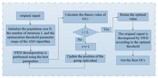
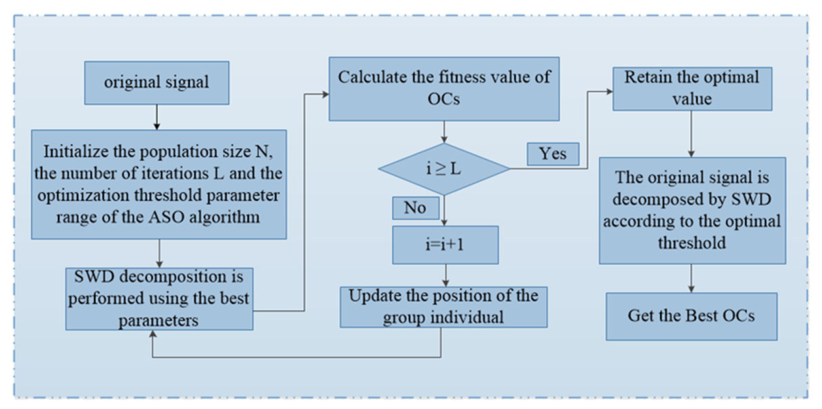
The ISWD algorithm proposed in this paper is illustrated in Figure 1, and the detailed steps are given as follows.

Figure 1. ISWD flowchart.

(1)

The original signal $x\left[n\right]$ is input and the algorithm parameters are initialized. By analyzing the vibration characteristics of the reciprocating compressor valve signal, the value ranges of Pth and StDth are set to [0.01, 0.9] and [0.01, 0.9], respectively. For the ASO algorithm, the population size N is set to 20 and the number of iterations L is set to 30.

(2)

The energy spectrum of the signal is calculated, the optimal frequency band is estimated, and the group parameters $\delta$ and M are initialized.

(3)

The iterative decomposition of SWD is performed, the current optimal individual is updated, the fitness value of the oscillatory component in each iteration is calculated, and the current optimal parameter combination is obtained.

(4)

If the number of iterations reaches the maximum value, the iteration is terminated and the optimal parameter combination is output.

(5)

The original signal is decomposed by SWD according to the optimal parameter combination, and all oscillatory components are obtained.

2.2. Feature Fusion

Before pattern recognition is performed using a classifier, the features of vibration and acoustic emission multi-source signals that characterize the different operating states of reciprocating compressor valves must first be extracted. Traditional linear analysis methods, due to their simple models, cannot simultaneously consider the low-frequency impact characteristics of vibration signals and the high-frequency defect characteristics of acoustic emission signals. It is difficult to fully capture the nonlinear and non-stationary properties of multi-source heterogeneous signals, resulting in one-sided feature representation [24], which directly reduces the accuracy of subsequent pattern recognition. As an effective nonlinear evaluation method, information entropy can quantitatively evaluate difficult-to-measure indices including equipment operation complexity and fault evolution rules [25] and can accurately characterize feature differences in multi-source signals under different fault conditions. Accordingly, permutation entropy, approximate entropy and time-domain energy entropy are selected based on entropy theory to extract fused features from multi-source signals, so as to build feature vectors that fully reflect valve working conditions.

(1)

Permutation Entropy

Permutation entropy describes the complexity of a time series or signal measured on a physical system and can be used as a nonlinear evaluation indicator for dynamic changes in equipment operating status [26], as shown in the following equation.

$$E_{PE}=-{\displaystyle \sum _{i=1}^{N}p\left(i\right)\ln p\left(i\right)}$$

(12)

In the formula, $E_{PE}$ denotes the permutation entropy value and $p_i$ denotes the occurrence probability of each sequence of the signal.

Approximate entropy is essentially regarded as a statistic related to time-series parameters; it can predict the probability of new modes being generated with variations in the signal sequence. The more complex the signal is, the higher the probability of new modes being generated and the more complex the corresponding approximate entropy will be, as shown in Equation (16).

$$ApEn\left(m,r,N\right)={\mathsf{\Phi }}^m\left(r\right)-{\mathsf{\Phi }}^{m+1}\left(r\right)$$

(13)

To achieve satisfactory pseudo-error and statistical properties, the dimension m is set to 2 and the threshold r is set within the range of 0.1–0.25 [26].

(2)

Time-domain Energy Entropy

The complexity and uncertainty of signal energy in the time domain are reflected by time-domain energy entropy, as shown in the following equation.

$$E_i=-{\log }_2\left({\displaystyle \frac{q_i}{q}}\right)$$

(14)

The main purpose of adopting feature fusion in this paper is to utilize different features to refine the information of various signal states. The above three types of information entropy are employed to characterize state features from different perspectives. The t-SNE algorithm, as a nonlinear manifold-learning dimensionality reduction algorithm, is capable of mapping high-dimensional data into low-dimensional space. Its processed data conforms to a t-distribution, which effectively relieves data crowding during dimension reduction [27]. After extracting multiple entropy features from the valve vibration signal, t-SNE is applied for feature fusion and dimensionality reduction. The obtained feature set can more comprehensively reflect the signal state information.

In this work, t-SNE is not merely adopted for two-dimensional or three-dimensional feature visualization. More importantly, it is introduced to realize the dimensionality reduction and fusion of high-dimensional heterogeneous features extracted from vibration and acoustic emission multi-source signals.

Multi-source signal fusion will generate a high-dimensional nonlinear feature distribution, and linear dimensionality reduction methods such as PCA struggle to mine the inherent manifold structure among fault samples. As a nonlinear manifold-learning method, t-SNE can effectively retain the local neighborhood relationship of high-dimensional multi-source features, reduce redundant interference information, and significantly improve the separability of different fault-state samples.

Therefore, t-SNE serves as an indispensable feature optimization link in this multi-source fault diagnosis framework, providing low-dimensional discriminative feature input for the subsequent MCNN-BiGRU classification model.

2.3. MCNN-BIGRU Model

Multi-scale Convolutional Neural Networks (MCNNs) are regarded as an extended form of Convolutional Neural Networks (CNNs). Their core advantage is reflected in their multi-input-channel and multi-branch parallel structure, which can be precisely adapted to the feature extraction requirements of multi-source heterogeneous signals, including the vibration and acoustic emission signals of reciprocating compressor valves. On the one hand, the multi-channel input architecture of the MCNN is adopted to support the simultaneous processing of two types of multi-source heterogeneous data, namely low-frequency impact vibration signals and high-frequency acoustic emission signals, and the feature extraction of multi-source signals is realized [28]. On the other hand, different convolution kernel sizes and parameters are configured for each branch, so that fault features of different scales can be extracted in a targeted manner. Sudden signal changes caused by valve wear and micro-leakage can be captured by small-scale convolution kernels, while macro vibration trends induced by valve jamming and fracture can be characterized by large-scale convolution kernels. Finally, branch feature fusion is utilized to effectively enhance feature diversity, and the ability of the model to capture the complex fault modes of compressor valves is greatly improved [29].

The multi-scale feature fusion of the MCNN is regarded as the core of its forward inference. Features of different scales are extracted through multi-branch convolution and weighted fusion is performed to generate the target output:

$$\widehat{D}={\displaystyle {\sum }_{l\in \left\{L,M,S\right\}}{\alpha }_l·\left(W_l\ast x_l+b_l\right)}$$

(15)

In the formula, $\widehat{D}$ denotes the density map predicted by the model (which can be replaced with a fault feature map in fault diagnosis scenarios); L, M, and S represent the large-, medium-, and small-scale convolution branches, respectively. ${\alpha }_l$ denotes the feature fusion weight of each scale branch.

The L2 loss function, which serves as the core of backward optimization, is used as the basis for model parameter updating. Optimization is achieved by minimizing the discrepancy between the predicted values and true values:

$$L={\displaystyle \frac{1}{2N}}{\displaystyle \sum _{i=1}^N{‖{\widehat{D}}_i-D_i^{\ast }‖}_2^2}$$

(16)

In the formula, L denotes the global loss value and N denotes the number of samples in a training batch; ${\widehat{D}}_i$ denotes the predicted density map or feature map of the i-th sample; $D_i^{\ast }$ denotes the true density map or label feature map of the i-th sample.

A Bidirectional Gated Recurrent Unit (BiGRU) is regarded as an optimized variant of a Recurrent Neural Network (RNN) and is designed specifically for the deep modeling of time-series data and is highly compatible with the temporal characteristics of the multi-source signals of compressor valves. On the one hand, the bidirectional propagation structure of the BiGRU is adopted to simultaneously mine the forward evolution law and backward correlation information of valve signal sequences, such as by capturing the evolution trajectory of fault features in the full cycle of valve opening, stabilization and closing, so that the problem that traditional unidirectional models barely take temporal front-to-back dependencies into account is effectively solved. On the other hand, the update gate and reset gate built into the model are used to intelligently regulate information flow, by which the key temporal characteristics of valve faults are retained and redundant noise is filtered, and the gradient vanishing problem in long-sequence training is significantly alleviated. Compared with Long Short-Term Memory (LSTM) networks, the BiGRU is equipped with fewer parameters and higher computational efficiency, so it is more suitable for processing the medium-length multi-source time-series signals of compressor valves, and the speed of model training and inference is improved while diagnostic accuracy is guaranteed [30].

The essence of the BiGRU, which enables the simultaneous capture of forward and backward time-series information, is reflected in the achievement of feature complementation by concatenating the hidden states of bidirectional GRUs:

$$h_t^B=Concat\left({\overrightarrow{h}}_t,\overleftarrow{h_t}\right),\left\{\begin{array}{l}{\overrightarrow{h}}_t=GRU\left({\overrightarrow{h}}_{t-1},x_t\right)\\ \overleftarrow{h_t}=GRU\left(\overleftarrow{h_{t+1}},x_t\right)\end{array}\right.$$

(17)

In the formula, h denotes the bidirectionally fused hidden state at time t (the core feature of the BiGRU); Concat(⋅) denotes feature concatenation and weighted fusion; and GRU(⋅) denotes the internal computation of the Gated Recurrent Unit.

Although this task only involves three-state fault classification of compressor valves, it faces the inherent complexity of vibration–acoustic emission multi-source heterogeneous signals. Simple shallow classification models struggle to simultaneously extract multi-scale spatial features from dual-channel signals and capture the periodic temporal correlation of reciprocating compressor operation.

The MCNN adopts multi-branch parallel convolution, which can adaptively mine multi-scale local feature differences contained in vibration and acoustic emission signals. The BiGRU is introduced to model the bidirectional temporal dependencies of forward and backward time-series multi-source data. Therefore, the MCNN BiGRU architecture is a targeted design for the characteristics of multi-source signals. It can fully explore the complementary fault information hidden in dual-channel signals, improving the accuracy and universality of fault diagnosis.

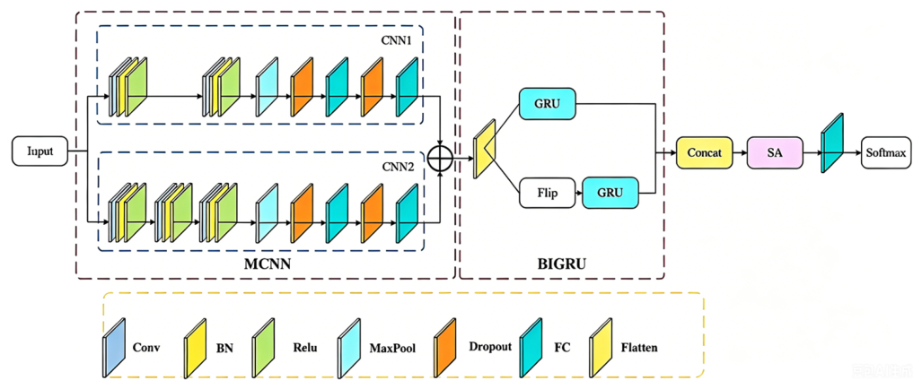
The detailed network architecture and training hyperparameters are supplemented as follows: the MCNN is composed of three parallel convolution branches with kernel sizes of 1 × 3, 1 × 5 and 1 × 7. The BiGRU adopts two layers with 64 hidden units. The fully connected layer is set to 128 neurons. ReLU is used as the activation function. The Adam optimizer is adopted with an initial learning rate of 0.001, a batch size of 16, and a maximum training epoch of 100. The rationality of the above structure and parameter setting is further verified by the ablation study in Section 4.3.

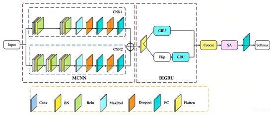
The diagnostic model of the MCNN-BiGRU is shown in the following Figure 2.

Figure 2. Diagnostic model of MCNN BiGRU.

2.4. ISWD-t-SNE-MCNN-BIGRU Fault Diagnosis Model

To accurately realize the fault pattern recognition and prediction of reciprocating compressor valves, this section integrates Improved Synchrosqueezing Wavelet Decomposition (ISWD), t-SNE dimensionality reduction and fusion, and the MCNN-BiGRU model to construct a fault diagnosis system adapted to vibration–acoustic emission multi-source signals. The proposed integrated framework is specially designed to address the characteristics of multi-source heterogeneous signals (vibration and acoustic emission) from reciprocating compressor valves. The ISWD algorithm is used to achieve adaptive, high-precision decomposition of multi-source non-stationary signals. The t-SNE method is applied to fuse and reduce high-dimensional heterogeneous features from vibration and acoustic emissions. The MCNN-BiGRU model is used to capture multi-scale spatial features and bidirectional temporal dependencies hidden in multi-source signals. This combination is not a simple superposition of methods, but a targeted design for multi-source signal characteristics. Each module serves an irreplaceable role in processing multi-source signals, improving feature separability, and enhancing diagnostic accuracy. The necessity and effectiveness of each component are verified by the ablation study in Section 4.3.

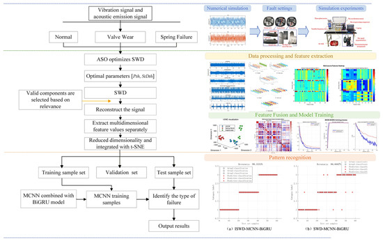
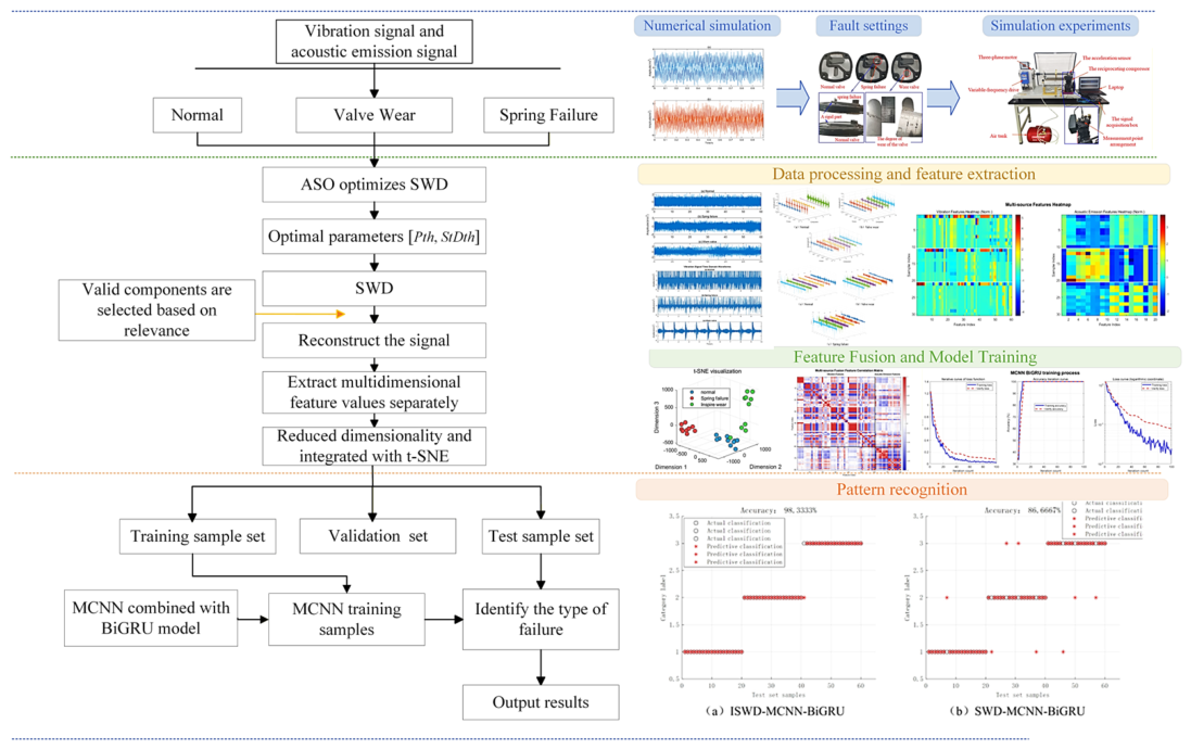
Relying on the efficient decomposition and denoising capabilities of ISWD for multi-source non-stationary signals, the oscillation components related to valve faults can be accurately extracted and the signals reconstructed, and then an initial feature set is constructed through the fusion of multiple entropy features. Combined with the advantages of the t-SNE algorithm concerning dimensionality reduction and the fusion of high-dimensional features, redundant information is eliminated and fault-sensitive features are strengthened. Finally, the powerful multi-scale feature capture and temporal dependency modeling capabilities of the MCNN-BiGRU model are utilized to achieve accurate recognition and prediction of fault patterns. The complete implementation process of this method (ISWD-t-SNE-MCNN-BiGRU) is shown in Figure 3.

Figure 3. Fault diagnosis process.

(1)

The original signals are input and the parameters of the SWD algorithm are initialized. The threshold ranges of Pth and StDth are set to [0.01, 0.9] and [0.01, 0.9], respectively.

(2)

The population size N and iteration number L of the ASO algorithm are set to 20 and 30, respectively. The SWD algorithm is optimized based on the ASO algorithm, and the optimal parameter combination is obtained. (Pth, StDth).

(3)

The original signals are decomposed by ISWD to obtain oscillation components (OCs), and the correlation coefficients between the OCs and the original signals are calculated.

(4)

The oscillation components (OCs) are screened according to the correlation coefficients, and the signals are reconstructed.

(5)

A total of 25 features, including the time-domain, frequency-domain and entropy features of the reconstructed signals, are extracted to form a feature set.

(6)

The feature set is fused by the t-SNE algorithm to obtain a low-dimensional feature set.

(7)

Next, 40% of the feature set is taken as the training set and input into the MCNN-BiGRU algorithm to construct and train the network model.

(8)

Finally, 10% of the feature set is used as the validation set, and the remaining feature set is taken as the test set. These sets are input into the network model constructed and trained above for pattern recognition to determine the types of faults, thus completing the entire fault recognition process.

3. Numerical Simulation Analysis

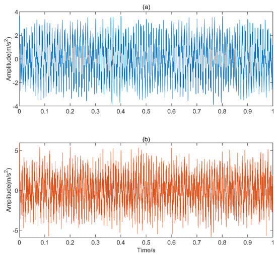
To evaluate the decomposition efficiency and feature extraction accuracy of the proposed Improved Synchrosqueezing Wavelet Decomposition (ISWD) algorithm for vibration–acoustic emission multi-source coupled signals, a periodic impact simulation signal is constructed in this paper, and white noise is added to the signal. It is expected that the signal can simultaneously contain the low-frequency vibration features corresponding to the valve opening and closing impacts and the high-frequency acoustic emission features generated by defect evolution and superimpose the measured background noise from industrial sites to simulate actual operating conditions. Its mathematical model is defined as shown in the formula below [31].

$$\left\{\begin{array}{l}{x}_1\left(t\right)=\left[0.2+0.3\cos \left(25\pi t\right)\right]\ast \sin \left(2\pi 80t\right)\\ x_2\left(t\right)=0.6\sin \left(2\pi 120t\right)+0.2\cos \left(2\pi 160t\right)\\ x_3\left(t\right)1.8\cos \left(2\pi 100t\right)\\ x_4\left(t\right)=1.2\sin \left(2\pi 350t\right)\\ x\left(t\right)=x_1\left(t\right)+x_2\left(t\right)+x_3\left(t\right)+x_4\left(t\right)\\ f\left(t\right)=x\left(t\right)+randn\left(size\left(x\left(t\right)\right)\right)\end{array}\right.$$

(18)

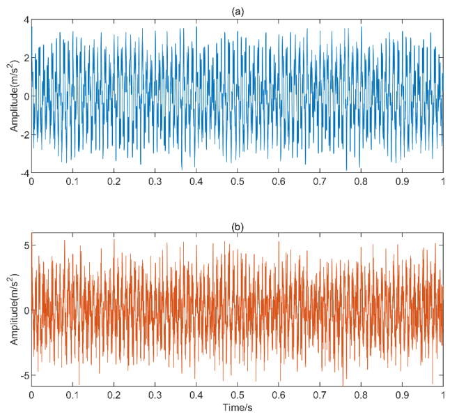
In the formula, the signal is composed of a modulated signal and signals with similar frequencies. The simulated signal is synthesized after adding Gaussian white noise. The dominant frequencies of the component signals are set to 80 Hz, 120 Hz, 160 Hz, 100 Hz, and 350 Hz, respectively. The length of the simulated signal is 5000, and the sampling frequency is 5000 Hz. The time-domain waveforms of the simulated signal before and after noise addition are shown in Figure 4.

Figure 4. Time–domain waveform of simulated signal. (a) No noise signal; (b) Simulated signal.

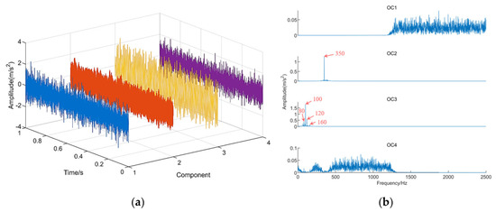
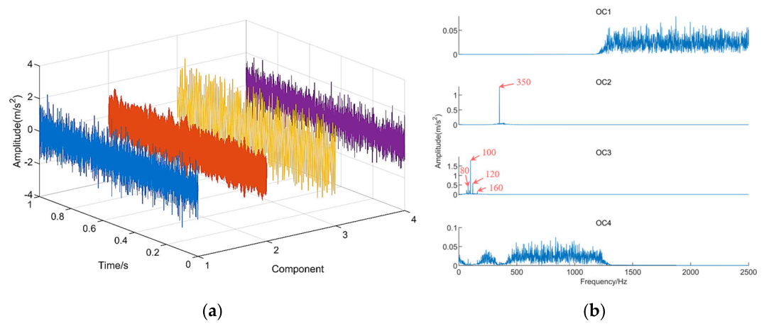
For the simulated signal, the optimal parameter combination (Pth, StDth) obtained by the ISWD method is calculated as (0.0468, 0.232). The simulated signal is decomposed using the ISWD method after parameter optimization, and the time-domain diagrams and frequency spectra of the obtained oscillation components are shown in Figure 5. The results show that four oscillation components are obtained by ISWD, which is consistent with the number of real signal sources, and the mode aliasing effect can be effectively avoided. In the frequency spectrum, the main frequencies of 80 Hz, 100 Hz, 120 Hz, 160 Hz and 350 Hz can be effectively extracted, as well as two sub-frequencies generated by modulation near 80 Hz. The main information of the simulated signal is well preserved, which proves that the ISWD method has good separation and extraction performance for modulated component signals.

Figure 5. ISWD results. (a) Time—domain waveform plot. (b) Spectrogram.

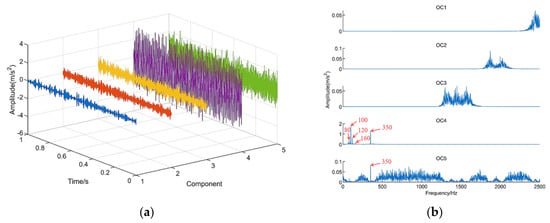
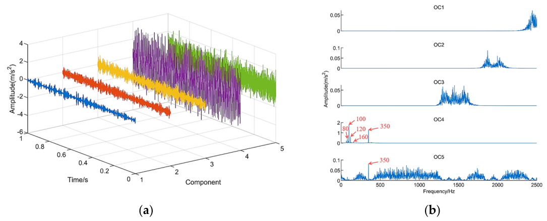
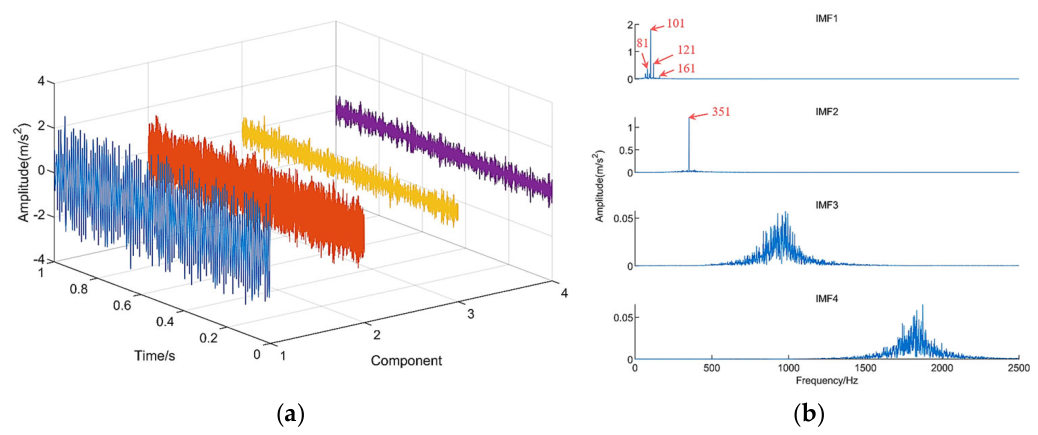
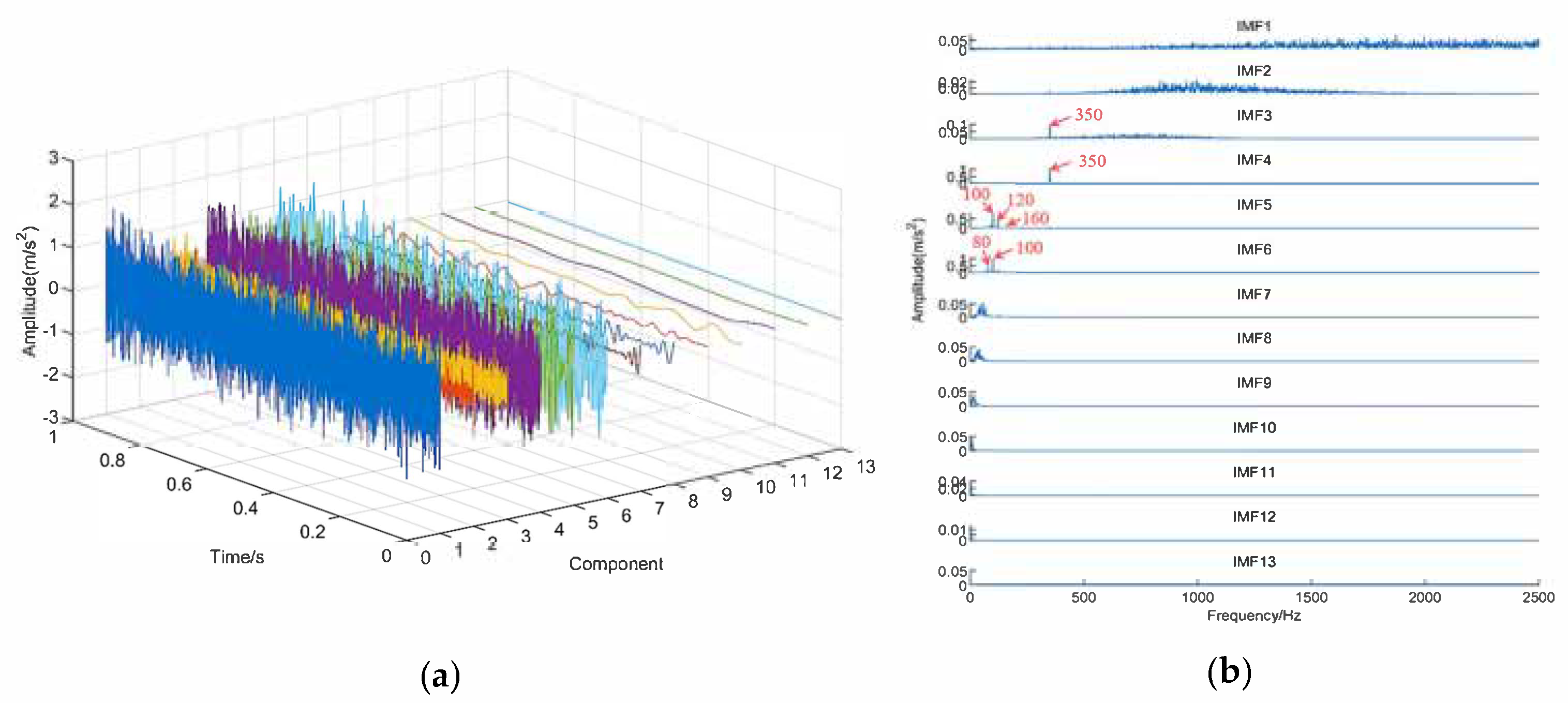
To further verify the advantages of the ISWD method, the decomposition results of the simulated signals produced using SWD, VMD, and CEEMDAN methods are compared. Among them, the default parameter combination (0.1, 0.1) is selected for the SWD algorithm. For the VMD algorithm, the number of decomposition modes is set as K = 4 and the quadratic penalty term is set as α = 2000 [32]. The results are shown in Figure 6, Figure 7 and Figure 8. It can be seen from Figure 6 that five oscillation components are obtained by SWD, resulting in redundant decomposition. The increase in oscillation components leads to longer computation time during decomposition. The frequency spectrum shows that SWD can effectively extract information from the signal components, but mode aliasing appears in OC5. Figure 7 shows that four components, namely Intrinsic Mode Functions (IMFs), are obtained by VMD, with no mode aliasing or redundant decomposition. However, the frequency spectrum reveals that the extracted frequencies differ by 1 Hz from the dominant frequencies of the simulated signal components. The threshold parameters of SWD and VMD must be manually selected and lack adaptivity. As shown in Figure 8, 13 components are generated after decomposing the simulated signal using CEEMDAN. Obvious over-decomposition results in numerous low-frequency and redundant components. In the spectrum of IMF6, two sub-frequencies generated by modulation near 80 Hz are missing, indicating unsatisfactory decomposition and extraction performance. The results demonstrate that the ISWD algorithm has certain advantages over other algorithms for decomposing and extracting multi-component modulated signals.

Figure 6. SWD results. (a) Time—domain waveform plot. (b) Spectrogram.

Figure 7. VMD results. (a) Time—domain waveform plot. (b) Spectrogram.

Figure 8. CEEMDAN decomposition results. (a) Time—domain waveform plot. (b) Spectrogram.

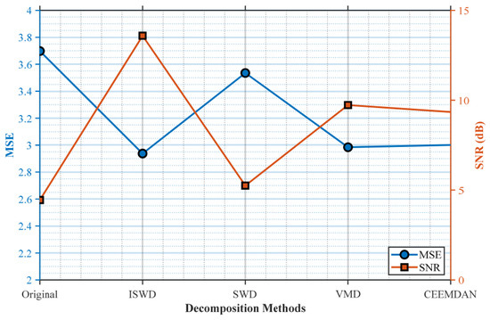
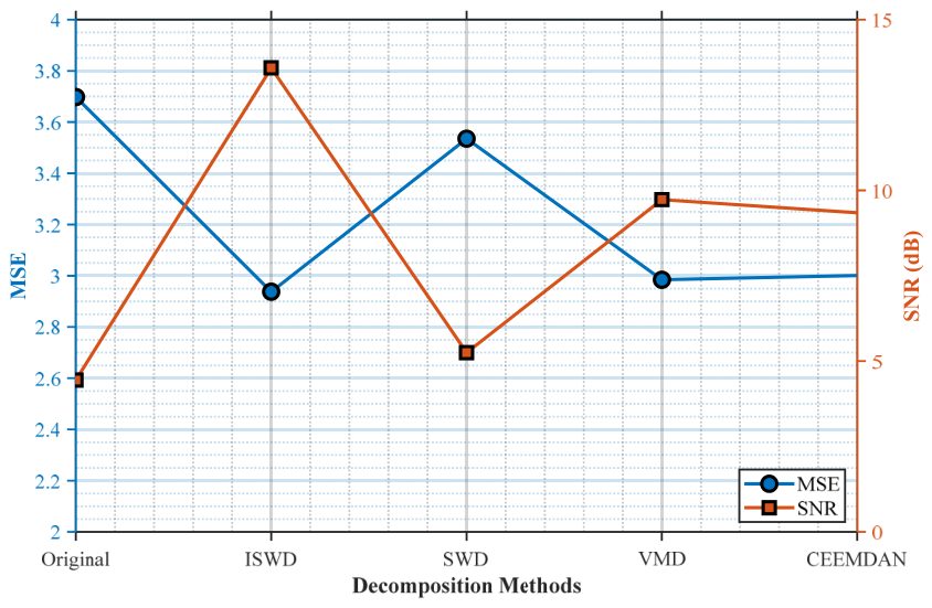
To further verify the denoising performance of the ISWD method, mean squared error (MSE) and signal-to-noise ratio (SNR) are introduced as performance evaluation metrics. MSE reflects the error between the true and estimated values of the signal and evaluates the degree of signal variation; a smaller MSE indicates a smaller signal deviation. SNR reflects the ratio of noise to effective information in the signal; a higher SNR indicates less noise contained in the signal. The calculation formulas are given as follows.

$$\left\{\begin{array}{l}MSE={\displaystyle \frac{1}{n}}{\displaystyle \sum _{i=1}^n{\left(X_i-\widehat{X}\right)}^2}\\ SNR=10{\log }_{10}\left({\displaystyle \frac{P_S}{P_N}}\right)=10{\log }_{10}{\displaystyle \frac{{‖X‖}^2/N}{MSE}}\end{array}\right.$$

(19)

In this paper, the correlation coefficients between the components decomposed by each method and the simulated signal are used as the judgment criterion to select the components with a high correlation with the original signal for signal reconstruction. The MSE and SNR values of the original simulated signal and the reconstructed signals processed by different methods are shown in Figure 9. In the figure, compared with the SWD, VMD and CEEMDAN algorithms, the reconstructed signal using the ISWD method has the smallest MSE value and the largest SNR value, which verifies the superiority of this method in signal fidelity and shows the strongest robustness of the filtering effect.

Figure 9. Comparison of MSE and SNR between the original simulated signal and the reconstructed signal decomposed by different methods.

Based on the above analysis, the main information of multi-component modulated signals can be effectively decomposed and extracted by the ISWD method with strong denoising ability, with certain advantages over the traditional SWD, VMD and CEEMDAN methods.

4. Experimental Verification

4.1. Experimental Bench Set Up

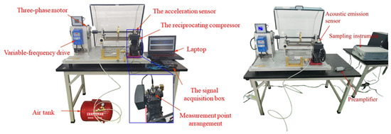
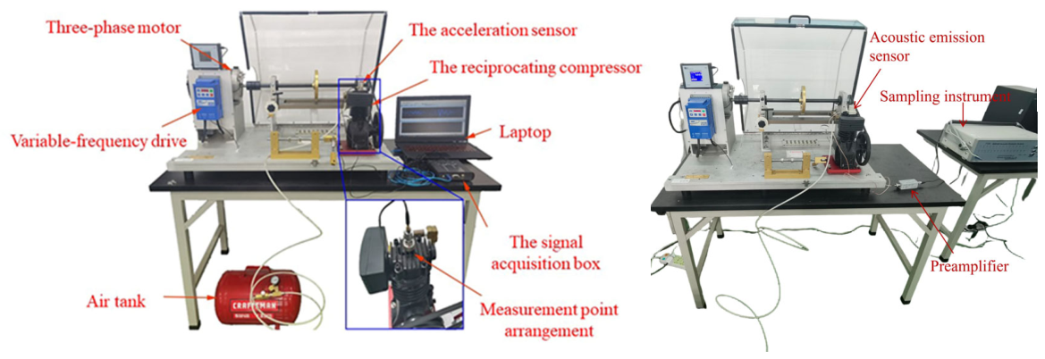
A reciprocating compressor experimental platform is built using the Spectra Quest mechanical fault simulation test bed, as shown in Figure 10, which is used to simulate normal valve conditions, intake valve wear, and exhaust valve spring failure. The equipment is a single-piston reciprocating compressor with a rated power of 367 W, a bore diameter of 5.08 cm, and stroke lengths of 5.08 cm and 3.81 cm. The maximum working pressure of the compressor is 0.86 MPa, and the volume flow rate is 0.07 m³/s at a pressure of 0.8 MPa. The compressor is driven by a shaft and a single-groove V-belt with a reduction ratio of 3.17. The compressor exhaust pipe is connected to an air storage tank to form a closed environment. The intake and exhaust valves are composed of two reeds, forming a cantilever beam structure.

Figure 10. Vibration simulation test bench for valve failure of reciprocating compressor.

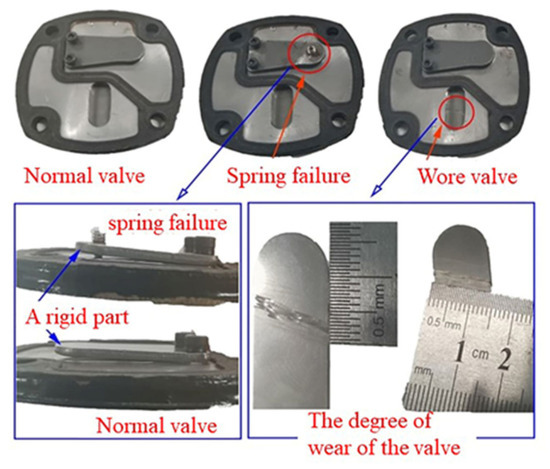
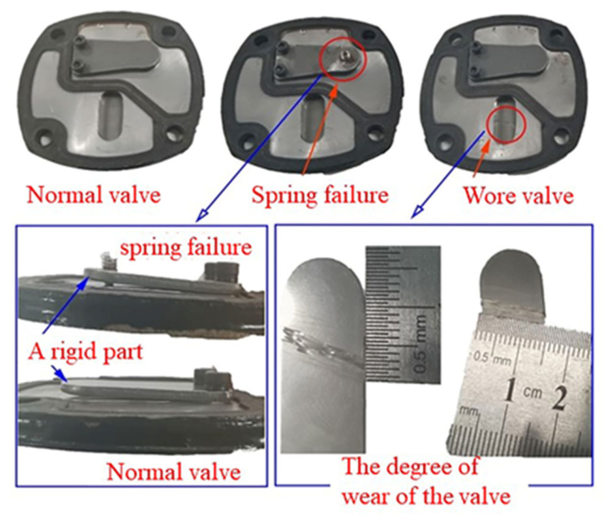
The details of the three working conditions (normal valve, intake valve wear, and exhaust valve spring failure) are shown in Figure 11. For the normal valve, the intake valve plate is smooth without any damage, and the exhaust valve plate can lift freely with no obstruction from the spring plate. Valve fault simulation is realized by adding a rigid component on the exhaust valve lift limiter to prevent the exhaust valve plate from lifting during operation and reduce its lift stroke, thus simulating the working condition of spring plate failure. For the intake valve, an artificial wear scar with a length of 14 mm and a width of 2 mm is processed to simulate the intake valve failure condition.

Figure 11. Simulation diagram of air valve malfunction.

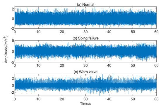
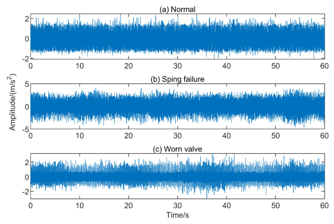
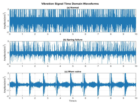
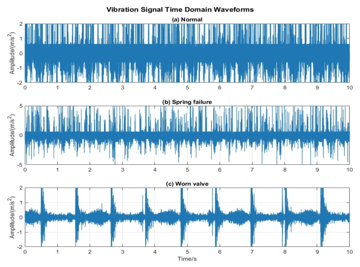
In this experiment, the IOtech640U data acquisition unit is adopted for vibration testing, equipped with a DH1A110E acceleration sensor with a sensitivity of 49.86 mV/g (equivalent to 5.088 mV/(m·s⁻²) after unit conversion). For acoustic emission testing, a G150 narrowband sensor (SR150M) is used, together with a PAI preamplifier with 40 dB gain and a DC 28 V power supply. All experiments are implemented in MATLAB R2023a. The computing environment is equipped with an Intel Core i9 processor and an NVIDIA GeForce RTX 4070 GPU. A uniform sampling frequency of 12,800 Hz and sampling points of 10,000 are set. Vibration signals under three operating conditions are collected at a motor rotating frequency of 20 Hz. A total of 60 s of data are recorded for each condition. The time-domain waveforms of the valve vibration signals and acoustic emission signals are shown in Figure 12 and Figure 13, respectively. It can be seen from the two figures that the vibration signals exhibit irregular periodic impacts, making it impossible to identify fault types from the time-domain waveforms. Some raw experimental and operational data are attached in the Supplementary Materials for reference.

Figure 12. Time–domain waveform of vibration signals for various operating conditions of the air valve. (a) Normal; (b) Spring failure; (c) Worn valve.

Figure 13. Time–domain waveform of acoustic emission signals for various operating conditions of the air valve. (a) Normal; (b) Spring failure; (c) Worn valve.

4.2. Data Analysis and Method Application

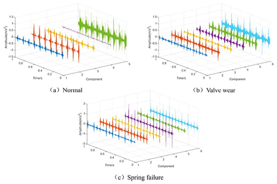
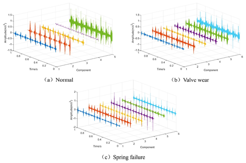
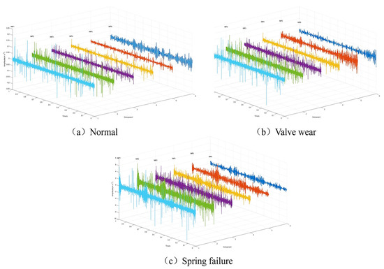
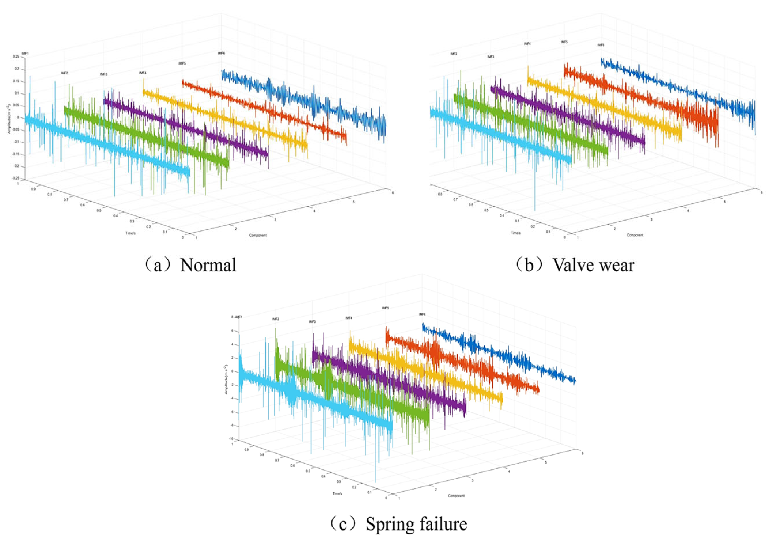
For the original vibration signals shown in the figures, the ISWD method is used for decomposition, and the obtained optimal parameter combinations are presented in Table 1. The optimal parameters are substituted into the SWD algorithm to decompose the corresponding original valve vibration signals, yielding the OC (oscillation component) modes of the signals under each operating condition. For clear waveform display and observation of the decomposition details, a typical segment of 12,800 data points is intercepted from the complete original signal for illustration. All subsequent feature extraction and model experiments are implemented based on the full-length original signal data. Taking 12,800 samples of each operating condition as an example, the OCs decomposed by ISWD are shown in Figure 14 and Figure 15: the normal valve signal is decomposed into five OCs, while both the spring failure and wear signals are decomposed into six OCs. The Pearson correlation coefficients between the OCs and the corresponding original vibration signals are calculated, and the OCs containing key state information are selected for signal reconstruction.

Table 1. Parameter values for each working condition.

Conditions	Optimal Parameters
	Pth	Stdth
The valve is normal	0.0147	0.115
Spring failure	0.0105	0.3254
Valve wear	0.0497	0.0718

Figure 14. ISWD results of vibration signal. (a) Normal; (b) Worn valve; (c) Spring failure.

Figure 15. ISWD results of acoustic emission signals. (a) Normal; (b) Worn valve; (c) Spring failure.

Multi-source vibration and acoustic emission samples are divided into three categories corresponding to the typical operating states of the air valve. In this work, a total of 60 samples are constructed, and each individual sample contains approximately 130,000 to 150,000 original data points with abundant fault characteristic information.

Permutation entropy, approximate entropy and time-domain energy entropy are extracted from the reconstructed multi-source signals of each sample. These three types of entropy features are fused to establish a multi-source feature set for valve fault diagnosis. After feature fusion and dimensionality reduction, the processed 60 feature samples are used for subsequent model training.

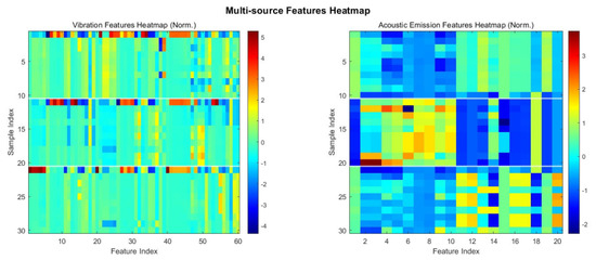
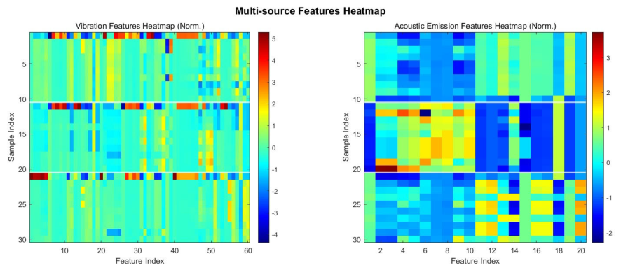
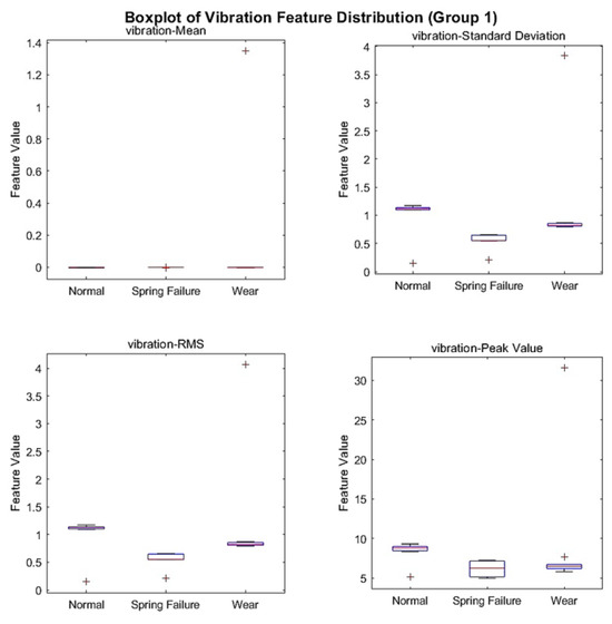
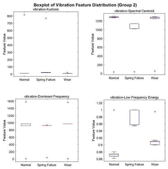
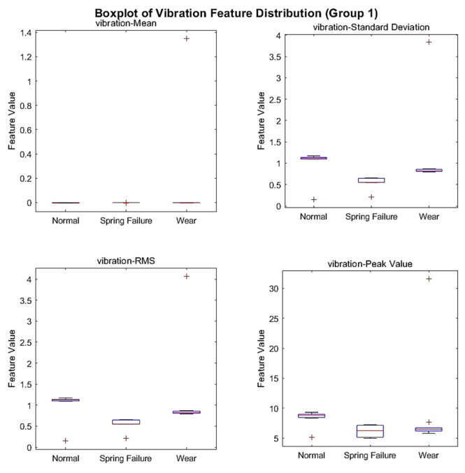
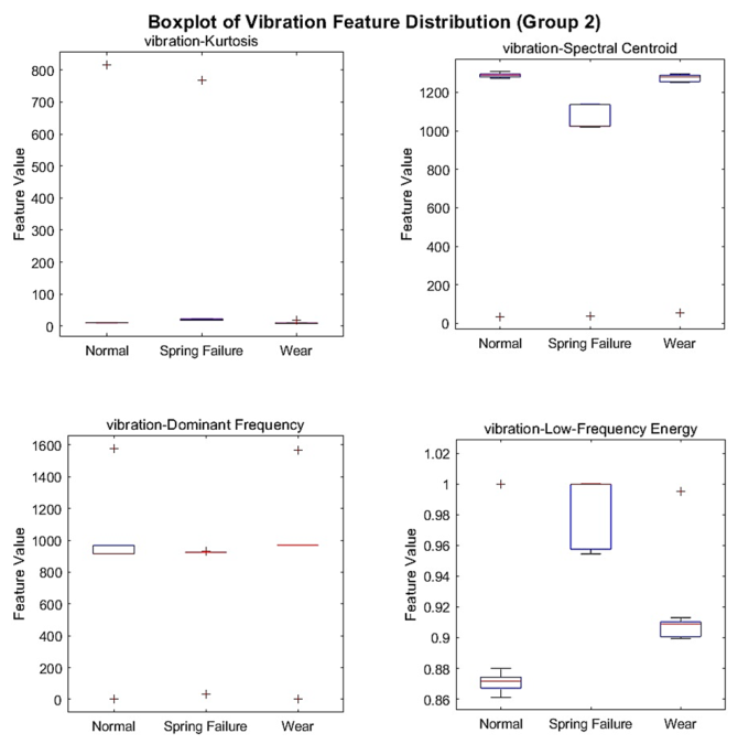
Given the high information density and complete temporal correlation of each long time-series sample, the 60 samples are sufficient to stably reflect typical fault features and operating patterns. Excessive segmentation destroys temporal correlation and introduces data redundancy, which is detrimental to model generalization. To ensure the generalization capability of the proposed method, repeated random division and multiple independent experiments are performed. Stable and consistent classification performance is maintained under different data partitions, thereby verifying the reliability of the model. Enabled by the powerful multi-scale feature learning and temporal modeling capabilities of the MCNN-BiGRU model, invariant fault characteristics can be effectively captured, thus guaranteeing strong generalization performance even with a limited number of high-information-density samples in real industrial scenarios. The heat maps and box plots of the multi-source features extracted from the vibration and acoustic emission signals are shown in Figure 16 and Figure 17.

Figure 16. Multi–source feature heat map.

Figure 17. Comparison box plot of vibration characteristic distribution.

Figure 16 and Figure 17 show the processed multi-source feature heat map, which directly presents the distribution differences in the multi-source signal feature values under different operating conditions and effectively verifies the effectiveness of the feature extraction strategy proposed in this paper. The left heat map shows the entropy feature distribution of the vibration signals under different valve states. From the interval division of the sample index, it can be seen that the sample blocks corresponding to different operating states such as normal, wear and leakage (e.g., sample index intervals 0–10, 10–20, 20–30) show obvious color differentiation along the feature index dimension. Some features (e.g., feature indices 10–15, 40–45) exhibit significant high red values or low blue values in fault-state samples, forming a strong contrast with the light green background of normal-state samples. This phenomenon indicates that the extracted vibration entropy features can effectively capture the macroscopic impact signal variations caused by valve faults, and the feature values under different states are distinguishable, verifying the effectiveness of vibration feature extraction. The right heat map corresponds to the entropy feature distribution of the acoustic emission signals, with more remarkable state distinguishability: in fault-state sample blocks (e.g., sample index intervals 10–20, 20–30), the region of feature indices 6–12 shows obvious high values from yellow to red, while normal-state samples are dominated by low blue values. This difference reflects that acoustic emission entropy features can accurately capture high-frequency signal changes generated by the evolution of microscopic valve defects such as wear and failure, complementing the macroscopic impact information of vibration features, which further proves the rationality and effectiveness of multi-source feature extraction.

By comparing the heat maps on both sides, obvious differences can be observed in the sensitive feature indices between the vibration features and acoustic emission features under different states. Vibration features focus more on reflecting the low-frequency time-domain variations caused by valve opening and closing impacts, while acoustic emission features concentrate on high-frequency signal changes in microscopic defects. The differentiated distribution of the two types of features indicates that the multi-source features extracted in this study can characterize the operating state of the valve relatively completely from both the macroscopic and microscopic dimensions, providing highly distinguishable input features for subsequent fault pattern recognition and fully verifying the success of the proposed feature extraction strategy.

The vibration feature box plot in Figure 17 intuitively shows the distribution differences in each feature under three conditions: normal conditions, spring failure, and valve wear. It can be seen from the figure that the value distributions of the kurtosis, waveform factor, root mean square and other features under fault conditions are significantly separated from those under normal conditions. For example, the box positions of the waveform factor and kurtosis under spring failure and valve wear conditions obviously deviate from those under normal conditions, and the value intervals of some features hardly overlap, indicating that the extracted vibration features can effectively distinguish different operating states of the valve and provide highly distinguishable input features for subsequent fault pattern recognition.

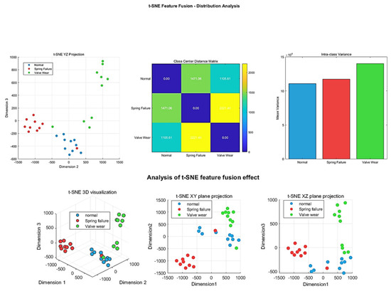
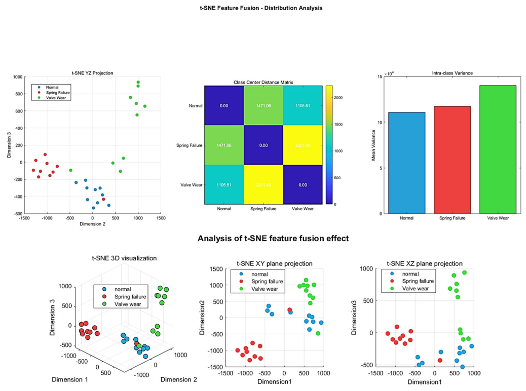
The t-SNE algorithm is adopted for feature fusion and dimensionality reduction. The extracted multi-source signal features are input into t-SNE for fusion, and the obtained results are shown in the following figure:

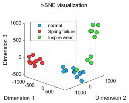
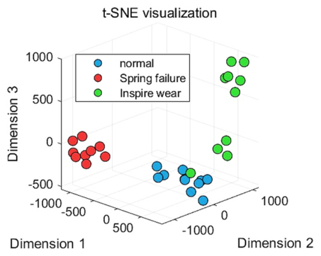
Figure 18 and Figure 19 show the two-dimensional visualization results of multi-source features after dimensionality reduction by t-SNE. It can be seen that the sample points representing the three states of normal conditions, exhaust valve spring failure, and intake valve wear form a distribution pattern with intra-cluster compactness and significant inter-cluster separation in the two-dimensional space. The exhaust valve spring failure samples (red) are concentrated in the left area, the intake valve wear samples (green) are clustered in the lower right area, and the normal samples (blue) are located in the upper right area. The feature clusters of the three types of samples hardly overlap.

Figure 18. Effect diagram of t-SNE feature fusion.

Figure 19. Multi–source feature t-SNE fusion result.

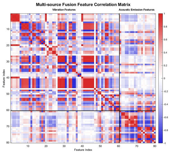
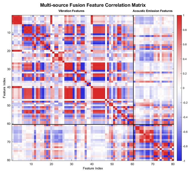
Figure 20 shows the heat map of the correlation matrix for the multi-source fused features. As can be seen from the figure, the vibration feature region and the acoustic emission feature region are divided by a red solid line, and the color transitions from dark blue (negative correlation, r = −1) to deep red (positive correlation, r = 1), which directly represents the pairwise correlation coefficient distribution of the vibration and acoustic emission multi-source features. It can be observed that some highly correlated features exist within the vibration features, while the correlation between most features is moderate or low. The internal correlation of the acoustic emission features is generally weak, mainly displayed in light colors, indicating that both types of single-modal features contain complementary fault information without serious information redundancy. Moreover, the cross-modal correlation between the vibration features and acoustic emission features is generally weak, further demonstrating that the fault information carried by macroscopic vibration and microscopic acoustic emission features is significantly complementary. Such a correlation distribution not only ensures the information complementarity within single-modal features but also realizes the effective fusion of multi-source information through low cross-modal correlation.

Figure 20. Multi–source feature correlation matrix.

The above feature fusion results show that the multi-source feature fusion strategy in this study can effectively extract differentiated features of different fault states. While effectively representing the original signals, it can still maintain high distinguishability after dimensionality reduction by t-SNE, laying a solid foundation for the accurate fault identification of the subsequent MCNN-BiGRU model.

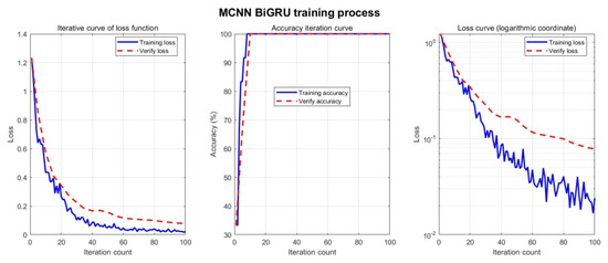
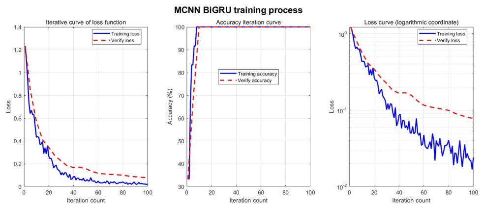
To eliminate the contingency of a fixed dataset partition, all feature samples are randomly divided. Among them, 40% are selected as the training set, 10% as the validation set, and the remaining 50% as the test set. In addition, 5-fold cross-validation is adopted in all experimental runs, and the averaged results from repeated tests are presented to further guarantee the stability and reliability of the diagnostic performance. To verify the effectiveness and superiority of the proposed method, comparative analyses are conducted using different methods. To ensure comparability, the features extracted by each method are kept consistent: the unoptimized SWD algorithm is used to decompose signals, and three types of information entropy are extracted and fused to form a feature set, which is then input into the MCNN-BiGRU model; the permutation entropy, approximate entropy, and time-domain energy entropy of signals processed by the ISWD method are extracted separately as the input feature set and fed into the MCNN-BiGRU algorithm. The iteration curve of the training process is shown in Figure 21, and the final fault recognition rate is also presented in Figure 21. The main hyperparameter settings of the proposed MCNN BiGRU model are shown in Table 2:

Figure 21. MCNN–BiGRU training process.

Table 2. Parameter setting of MCNN BiGRU model.

Parameter	Value
Number of convolution filters	32
Convolution kernel sizes	[3, 5, 7]
Number of GRU units	64
Dropout rate	0.3
Optimizer	Adam (MATLAB R2022a default)
Initial learning rate	0.001
Mini-batch size	16
Maximum training epochs	100

The convergence characteristics and generalization ability of the MCNN-BiGRU model are clearly demonstrated in Figure 21. The loss function iteration curve on the left indicates that both training the loss and validation loss decrease rapidly with increasing iterations and tend to be stable after about 40 iterations. The two curves fit well without obvious deviation, demonstrating that the model converges fast and no overfitting occurs. The accuracy iteration curve in the middle shows that training accuracy and validation accuracy rise rapidly and synchronously and finally stabilize at a level close to 100%, reflecting the model’s excellent fitting ability for fault features. The loss curve under the logarithmic coordinates on the right further verifies the stability of model convergence. The loss value shows a continuous downward trend and tends to be stable on the logarithmic scale with only slight fluctuations. Overall, the model training process is stable with fast convergence and good generalization ability, which provides a solid guarantee for the accuracy of subsequent fault diagnosis.

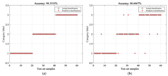
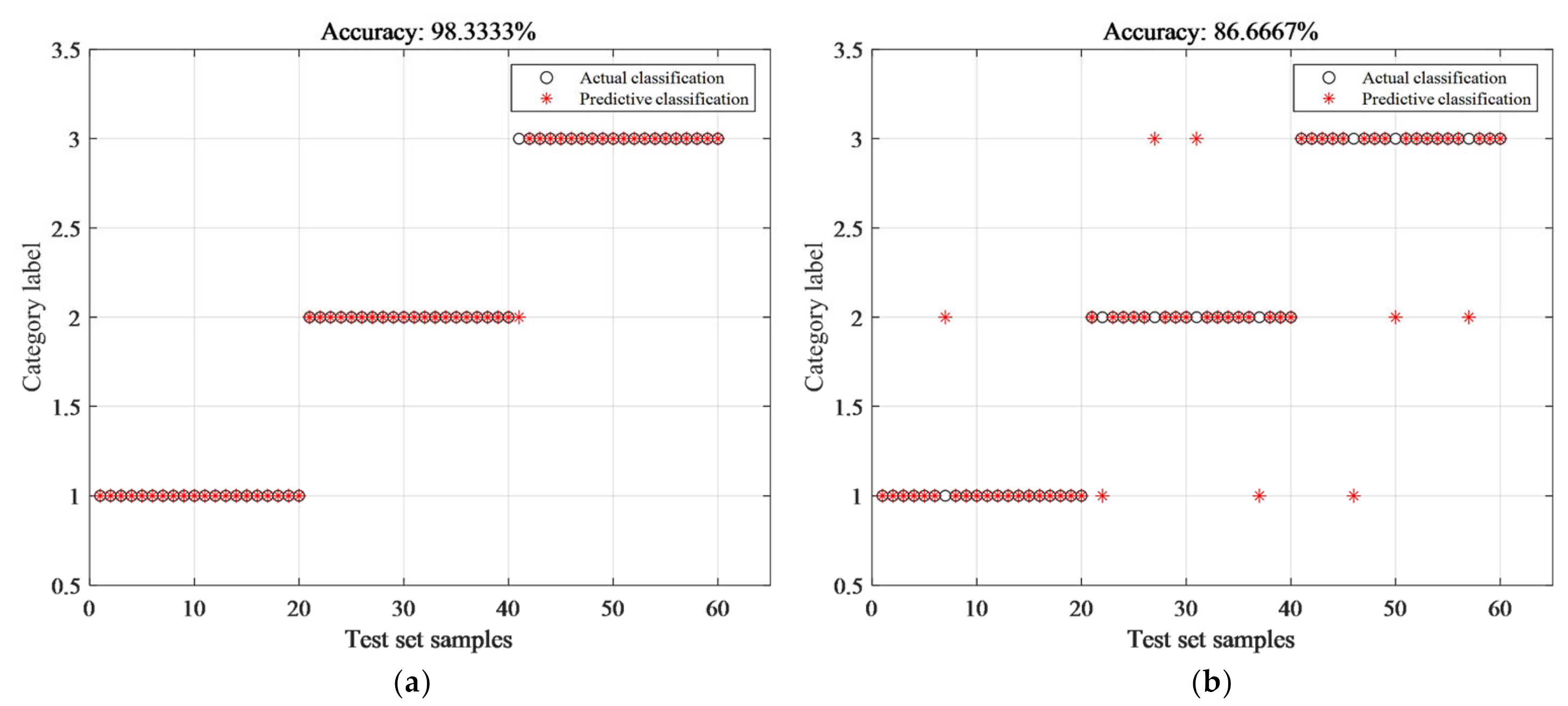
It can be seen from Figure 22 that after inputting the multi-source fused feature set into the MCNN-BiGRU model, the fault classification accuracy of multi-source signals processed by the ISWD algorithm reaches 98.3%, which is significantly higher than 86.67% obtained by the original SWD algorithm. This fully verifies that the ISWD optimization method proposed in this paper effectively improves the decomposition and feature extraction performance for multi-source non-stationary signals and can more accurately mine fault-sensitive information and filter out industrial background noise from multi-source signals.

Figure 22. Fault diagnosis results. (a) Result of ISWD-MCNN-BiGRU model; (b) Result of SWD-MCNN-BiGRU model.

4.3. Ablation Study

To quantitatively verify the effectiveness and necessity of each core module contained in the proposed model, a series of ablation experiments are conducted following the controlled-variable principle. Three comparative baseline models are constructed by individually removing the t-SNE feature fusion module, the ISWD feature screening module and the BiGRU temporal modeling module from the overall framework. All comparison experiments are implemented under identical experimental constraints, including the same dataset, hyperparameter setting and training optimization strategy. Loss convergence curves, integrated confusion matrices and quantitative evaluation metrics are adopted as comprehensive assessment indices. The influence of each key module on the training convergence stability, feature representation capability and fault classification performance is systematically analyzed.

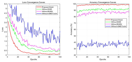
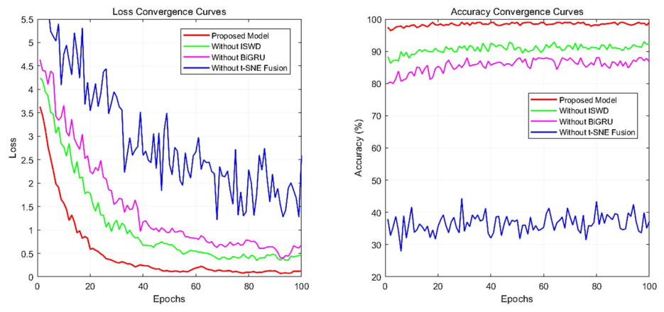
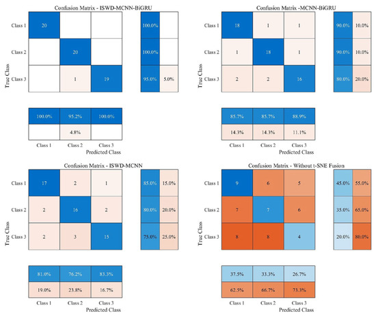
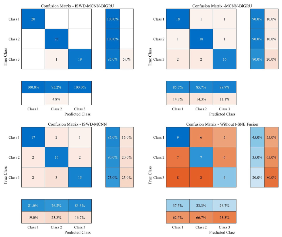
The loss convergence curves of the proposed complete model and all ablation models are illustrated in Figure 23. The overall classification performance of all four models is intuitively displayed in Figure 24, where four confusion matrices are integrated into a single subplot layout. The quantitative comparison results of the diagnostic metrics for all models are listed in Table 3. The overall classification accuracies of the model without ISWD, the model without t-SNE fusion, the model without the BiGRU, and the proposed complete model are calculated as 86.67%, 33.33%, 80.00%, and 98.33%, respectively. The optimal diagnostic accuracy is obtained by the full proposed model.

Figure 23. Loss convergence curves of the proposed model and ablation models.

Figure 24. Confusion matrices of the proposed model and three ablation models.

Table 3. Quantitative comparison of diagnostic metrics for different models.

Model	Accuracy (%)	Precision (%)	Recall (%)	F1-Score (%)
Method proposed	98.33	96.44	98.33	96.27
Without ISWD	86.67	90.48	86.67	87.04
Without t-SNE	33.33	11.11	33.33	16.67
Without BiGRU	80.00	84.92	80.00	77.13

From the perspective of the loss convergence characteristics, when the ISWD module is removed, slight attenuation is observed in both convergence performance and classification accuracy. It is noted that the ISWD module is mainly employed for signal decomposition and reconstruction rather than simple feature screening. Complex original monitoring signals are decomposed into multiple sub-signal components by this module, while invalid noise components are suppressed and effective fault-related components are reconstructed. The refined signal components can provide high-quality input for subsequent feature learning, so that the feature discrimination and diagnostic stability of the model are further improved.

When the t-SNE feature fusion module is removed, the loss curve is characterized by violent and continuous oscillation during the whole training process, and stable convergence cannot be achieved. The classification accuracy is maintained at the level of random guess, which demonstrates that the t-SNE dimensionality reduction and cross-source feature fusion module serves as the core foundation for mining effective hidden fault features from multi-source monitoring signals. Once this module is discarded, the high-dimensional feature space is disordered, and the basic fault classification capability of the model will be completely lost.

When the BiGRU temporal modeling module is eliminated, the convergence rate of the model significantly slows down, and obvious fluctuations are still observed in the middle and late training periods. The final classification accuracy is reduced sharply, which illustrates that a bidirectional gated recurrent structure can be adopted to capture the long-range temporal dependencies of sequential fault signals, and the representation ability of temporal dynamic features is effectively enhanced.

As can be observed from the integrated confusion matrix diagram (Figure 24), the number of misclassified samples is increased significantly, and the inter-class confusion degree is visibly increased when any core module is removed. The model without ISWD exhibits a moderate number of misclassified samples, while the model without BiGRU shows more serious category confusion. In particular, the model without t-SNE fusion presents completely disordered prediction results with massive misclassification across all categories, which is highly consistent with its extremely low classification accuracy. In contrast, the proposed complete model features earlier convergence speed and slighter late-stage oscillation in the loss curve. The predicted labels are highly consistent with the ground-truth labels, and the diagonal classification proportion of the confusion matrix is significantly higher than that of all ablation contrast models.

As listed in Table 3, the comprehensive quantitative metrics including the overall accuracy, precision, recall, and F1-score of the proposed model are all superior to those of the other three ablation models. It is verified that the removal of any key module will lead to an obvious decline in diagnostic performance.

In summary, the ISWD signal decomposition and reconstruction module, t-SNE feature fusion module, and BiGRU temporal modeling module are all proved to be indispensable for the proposed diagnostic model. Synergistic cooperation and complementary advantages are realized among the three modules, which jointly enhance the multi-signal decomposition ability, multi-source feature extraction ability, temporal dynamic modeling capability, training convergence stability, and intelligent fault diagnosis accuracy of the model. The rationality and advancement of the structural design of the proposed model are fully validated.

To further verify the effectiveness and superiority of the proposed method for multi-source signal fault diagnosis, entropy features extracted from multi-source signals decomposed and reconstructed by various decomposition algorithms are input into the MCNN-BiGRU and other neural network models for comparison, and the results are shown in Table 4. The above results fully indicate that the feature set extracted by the multi-source signal fusion of reciprocating compressor valves in this study effectively retains the core differentiated information under different fault states, eliminates a large amount of noise and redundant features in the multi-source signals, and significantly improves the overall performance of compressor valve fault diagnosis using multi-source signals.

Table 4. The fault recognition rate of different methods.

Model	Recognition Rate (%)
Method proposed in this paper	98.33%
ISWD-MCNN	86.67%
SWD-MCNN	85.18%
ISWD-CNN-LSTM	81.68%
SWD-CNN-LSTM	72.22%
Attention-CNN	93.33%
VMD-SVM	79.63%
Transformer	High data demand, poor performance

In addition to the above comparison methods, the proposed method was also compared with attention-based CNN and transformer methods, which are two representative advanced models in recent fault diagnosis research.

Due to the high complexity, large parameter scale, and high data requirements of transformer and attention models, their computational efficiency is low, their model training speed is slow, and, in this study, they are prone to overfitting with limited experimental samples. Therefore, their performance is inferior to the proposed lightweight and efficient MCNN BiGRU model.

5. Conclusions

To address the issues with extracting nonlinear and non-stationary features and identifying fault types from the multi-source signals of reciprocating compressor valves, this paper proposes a fault diagnosis model combining ISWD, multi-source entropy feature extraction, t-SNE dimensionality reduction, and MCNN-BiGRU. Numerical simulations and experimental results demonstrate that this method can accurately decompose multi-source signals and mine fault-sensitive information. Compared with traditional schemes, it significantly improves diagnostic efficiency and accuracy, providing a reference approach for the identification of typical valve faults.

The main findings of the fault diagnosis model used in this paper are as follows: (1) The multi-source signals of typical valve faults (intake valve wear, exhaust valve spring failure) show significant nonlinear characteristic differences from those in the normal state, and the numerical distribution of entropy features can effectively distinguish different operating states. (2) Single-signal decomposition or single-type feature extraction can hardly fully characterize multi-source fault information and tends to result in low diagnostic accuracy due to mode aliasing and feature redundancy. (3) Compared with traditional schemes such as SWD and VMD, the diagnosis model based on ISWD combined with multi-source feature fusion and MCNN-BiGRU achieves better decomposition and denoising effects on multi-source signals, higher fault classification accuracy, and more stable diagnostic performance.

Future Work

Future research will be further expanded and deepened on the basis of the existing work, in the following directions:

(1)

Fault types and operating condition coverage will be expanded, and complex working conditions including valve leakage, valve plate fracture, and multi-fault coupling will be introduced to enhance the generalization ability of the model in real industrial scenarios.

(2)

The model’s lightweight design and real-time inference capability will be optimized for edge-embedded devices, and transfer learning as well as few-shot learning will be adopted to tackle the scarcity of fault samples and high labeling costs, thus improving diagnostic performance with limited samples and under variable working conditions.

(3)

Physics-informed and data-driven fusion modeling will be combined to integrate compressor dynamic characteristics with deep learning feature extraction, and the t-SNE algorithm will be further optimized to improve the stability and reproducibility of multi-source feature dimensionality.

References

- Zheng, J.; Pan, H.; Yang, S.; Cheng, J. Adaptive parameterless empirical wavelet transform based time-frequency analysis method and its application to rotor rubbing fault diagnosis. Signal Process. 2017, 130, 305–314. [Google Scholar] [CrossRef] [Scilit]
- Zhang, Z.; Wang, W.; Chen, W.; Xiao, Q.; Xu, W.; Li, Q.; Wang, J.; Liu, Z. Fault Diagnosis of Reciprocating Compressor Valve Based on Triplet Siamese Neural Network. Machines 2025, 13, 263. [Google Scholar] [CrossRef] [Scilit]
- Guo, D.; Yang, X.; Peng, P.; Zhu, L.; He, H. The intelligent fault identification method based on multi-source information fusion and deep learning. Sci. Rep. 2025, 15, 6643. [Google Scholar] [CrossRef] [Scilit] [PubMed]
- Joseph, E.R.; Jakir, H.; Thangavel, B.; Nor, A.; Lim, T.L.; Mariathangam, P.R. Tool-emitted sound signal decomposition using wavelet and empirical mode decomposition techniques—A comparison. Symmetry 2024, 16, 1223. [Google Scholar] [CrossRef] [Scilit]
- Yu, Y.; Li, W.; Sheng, D.; Chen, J. A novel sensor fault diagnosis method based on Modified Ensemble Empirical Mode Decomposition and Probabilistic Neural Network. Measurement 2015, 68, 328–336. [Google Scholar] [CrossRef] [Scilit]
- María, E.T.; Marcelo, A.C.; Gast, S.; Patrick, F. A complete ensemble empirical mode decomposition with adaptive noise. In Proceedings of the IEEE International Conference on Acoustics, Speech and Signal Processing (ICASSP), Prague, Czech Republic, 22–27 May 2011. [Google Scholar]
- Bie, F.; Du, T.; Lyu, F.; Pang, M.; Guo, Y. An Integrated Approach Based on Improved CEEMDAN and LSTM Deep Learning Neural Network for Fault Diagnosis of Reciprocating Pump. IEEE Access 2021, 9, 23301–23310. [Google Scholar] [CrossRef] [Scilit]
- Guan, Y.C.; Tong, P.; Feng, Z.P. Fault current signal characteristic analysis of planetary gearbox based on ICEEMDAN method and frequency demodulation. J. Vib. Shock 2019, 38, 41–47. [Google Scholar]
- Chen, H.; Lu, L. An improved coverage optimization method for video sensor networks based on whale optimization algorithm. IEICE Electron. Express 2024, 21, 20230570. [Google Scholar] [CrossRef] [Scilit]
- Chegini, S.N.; Amini, P.; Ahmadi, B.; Bagheri, A.; Amirmostofian, I. Intelligent Bearing Fault Diagnosis using Swarm Decomposition Method and New Hybrid Particle Swarm Optimization Algorithm. Soft Comput. 2022, 26, 1475–1497. [Google Scholar] [CrossRef] [Scilit]
- Yang, R.X.; Xiong, R.; Shen, W. Research on thermal model of external short circuit for lithium-ion power battery in electric vehicle based on extreme learning machine. Engineering 2021, 7, 266–289. [Google Scholar] [CrossRef] [Scilit]
- Dragomiretskiy, K.; Zosso, D. Variational Mode Decomposition. IEEE Trans. Signal Process 2014, 62, 531–544. [Google Scholar] [CrossRef] [Scilit]
- Lu, H.; Du, B.; Liu, J.; Xia, H.; Yeap, W.K. A kernel extreme learning machine algorithm based on improved particle swam optimization. Memetic Comput. 2017, 9, 121–128. [Google Scholar] [CrossRef] [Scilit]
- Poongadan, S.; Lineesh, M.C. Non-linear time series prediction using improved CEEMDAN, SVD and LSTM. Neural Process. Lett. 2024, 56, 164. [Google Scholar] [CrossRef] [Scilit]
- Wu, S.L.; Zhou, Y.; Xing, W.T. Gearbox fault diagnosis method based on SDP and MCNN-LSTM. J. Vib. Shock 2024, 43, 126–132. [Google Scholar]
- Lu, N.; Zhou, T.X.; Wei, J.F.; Yuan, W.L.; Li, R.Q.; Li, M.L. Application of a whale optimized variational mode decomposition method based on envelope sample entropy in the fault diagnosis of rotating machinery. Meas. Sci. Technol. 2021, 33, 015014. [Google Scholar] [CrossRef] [Scilit]
- Li, K.; Wu, H.; Liu, X.; Xu, J.; Han, Y. Intelligent diagnosis of rolling bearing based on ICEEMDAN-WTD of noise reduction and multi-strategy fusion optimization SCNs. IEEE Access 2024, 12, 36908–36923. [Google Scholar] [CrossRef] [Scilit]
- Yan, R.; Liu, Y.; Gao, R.X. Permutation entropy: A nonlinear statistical measure for status characterization of rotary machines. Mech. Syst. Signal Process. 2012, 29, 474–484. [Google Scholar] [CrossRef] [Scilit]
- Yu, B. Research on Early Fault Diagnosis Method of Disc Tool Magazine Based on MCNN-BiGRU. Master’s Thesis, Jilin University, Changchun, China, 2025. [Google Scholar]
- Wei, W.; Wang, Z.H.; Liu, X.Q.; Feng, Z.; Li, J. Acoustic emission diagnosis of rolling bearing faults based on MDFF and ISSA. J. Vib. Shock 2023, 42, 65–76. [Google Scholar]
- Zheng, W.; Ai, Y.; Zhang, W. Improved Snake Optimizer Using Sobol Sequential Nonlinear Factors and Different Learning Strategies and Its Applications. Mathematics 2024, 12, 1708. [Google Scholar] [CrossRef] [Scilit]
- Zhou, J.; Shu, X.; Zhang, J.; Yi, F.; Jia, C.; Zhang, C.; Kong, X.; Zhang, J.; Wu, G. A deep learning method based on CNN-BiGRU and attention mechanism for proton exchange membrane fuel cell performance degradation prediction. Int. J. Hydrogen Energy 2024, 94, 394–405. [Google Scholar] [CrossRef] [Scilit]
- Tang, J.; Wu, J.; Hu, B.; Liu, J. An intelligent diagnosis method using fault feature regions for untrained compound faults of rolling bearings. Measurement 2022, 204, 112100. [Google Scholar] [CrossRef] [Scilit]
- Jiang, X.; Wang, J.; Shen, C.; Shi, J.; Huang, W.; Zhu, Z.; Wang, Q. An adaptive and efficient variational mode decomposition and its application for bearing fault diagnosis. Struct. Health Monit. 2020, 20, 2708–2725. [Google Scholar] [CrossRef] [Scilit]
- Ma, F.; Sun, W.; Jiang, Z.; Suo, S.; Wang, X.; Liu, Y. Industrial Robot Trajectory Optimization Based on Improved Sparrow Search Algorithm. Machines 2024, 12, 490. [Google Scholar] [CrossRef] [Scilit]
- Hu, Q.; Zhou, H.; Wang, C.; Zhu, C.; Shen, J.; He, P. Time-frequency fusion features-based GSWOA-KELM model for gear fault diagnosis. Lubricants 2023, 12, 10. [Google Scholar] [CrossRef] [Scilit]
- Li, J.; Wu, Y. Improved sparrow search algorithm with the extreme learning machine and its application for prediction. Neural Process. Lett. 2022, 54, 4189–4209. [Google Scholar] [CrossRef] [Scilit]
- Zhao, L.; Shi, H.; Zhao, W.T.; Li, Q.-H. Parameter Optimization of Washout Algorithm Based on Improved Sparrow Search Algorithm. J. Nanoelectron. Optoelectron. 2024, 19, 864–873. [Google Scholar] [CrossRef] [Scilit]
- Zhang, X.Q.; Wang, Z.N.; Li, J.S.; Liu, Y.H.; Chen, W.L. Identification of key nodes in temporal social networks based on deep learning and multi-feature fusion. Comput. Sci. 2026, 53, 143–154. [Google Scholar]
- Lyu, F.; Ding, X.; Li, Q.; Chen, S.; Zhang, S.; Huang, X.; Huang, W. Research on Fault Diagnosis Method of Reciprocating Compressor Based on RSSD and Optimized Parameter RCMDE. Appl. Sci. 2024, 14, 11556. [Google Scholar] [CrossRef] [Scilit]
- Zhang, S.Y.; Xu, M.Q.; Li, Y.B.; Zhao, H.Y.; Wang, R.X. Research on hybrid fault diagnosis method for reciprocating compressor valves. J. Vib. Shock 2016, 35, 167–173. [Google Scholar]
- Liu, Z.L.; Zhang, X.N.; Chen, Z.P.; Tang, Y.J.; Mei, S.Z.; Zhong, C.B.; Gu, X.M.; Zuo, M.J. Analysis method for homogeneous multi-source aliasing signals of booster cylinder in hydrogen compressor based on variational cyclic impact mode decomposition. J. Mech. Eng. 2026; ahead of print.
Disclaimer/Publisher’s Note: The statements, opinions and data contained in all publications are solely those of the individual author(s) and contributor(s) and not of MDPI and/or the editor(s). MDPI and/or the editor(s) disclaim responsibility for any injury to people or property resulting from any ideas, methods, instructions or products referred to in the content. |
© 2026 by the authors. Licensee MDPI, Basel, Switzerland. This article is an open access article distributed under the terms and conditions of the Creative Commons Attribution (CC BY) license.