Mapping Heavy Metals in Agricultural Soils Using a Hybrid HASM–ANN Model: A Case Study of the Eastern Longquan Mountain Region, China

Abstract

Mitigating heavy metal (HM) contamination in soil is vital for ecological and food security. Accurately mapping these pollutants and understanding their drivers are essential prerequisites for informed regional environmental governance. However, conventional spatial interpolation techniques used to estimate HM concentrations are susceptible to systematic biases and inadequate spatial resolution. To address these limitations, this study developed a novel hybrid model, termed HASM–ANN, coupling high-accuracy surface modeling (HASM) with artificial neural networks (ANNs). This approach generated high-resolution spatial distributions of HMs (As, Cd, Cu, Hg, Cr, and Pb) in agricultural soils of the Eastern Longquan Mountain region, Chengdu, China. Furthermore, the geographical detector (GD) and the Multiscale geographically weighted regression (MGWR) models were employed to explore driving mechanisms. Results indicate that HASM–ANN significantly outperformed conventional interpolations (ordinary/universal kriging, IDW) and HASM–coupled other machine learning downscaling methods. The proposed model demonstrated high predictive accuracy, yielding R² values between 0.75 and 0.86, and consistently achieved a significantly lower RMSE across all targeted soil heavy metals compared to the HASM. Analysis of the explanatory power (q) revealed that soil As was primarily influenced by clay content (CC, q = 0.45) and available phosphorus (AP, q = 0.42), whereas Cd was mainly driven by AP (q = 0.51) and PM_2.5 (q = 0.43). The spatial distribution of Hg was largely governed by soil organic matter (SOM, q = 0.53). Additionally, Cu concentrations were determined by SOM (q = 0.38), CC (q = 0.34), and pH (q = 0.31). Notably, Cr was significantly influenced by CC (q = 0.42), pH (q = 0.38), and elevation (q = 0.31), while Pb was further driven by SOM (q = 0.46) and PM_2.5 (q = 0.39). By offering high-precision mapping and elucidating the underlying driving mechanisms, this research directly facilitates informed environmental governance to protect ecological integrity and public health.

1. Introduction

Serving as a vital component of terrestrial ecosystems, soil is not only a prerequisite for agricultural production but also a critical resource underpinning global ecological sustainability [1]. In recent decades, heavy metal (HM) contamination in Chinese soils has emerged as a prominent environmental issue, garnering widespread research attention [2]. A review by Zhao et al. indicated that the presence of HMs in agricultural soils in China primarily involves Cadmium (Cd), Arsenic (As), Lead (Pb), and Mercury (Hg), while the accumulation levels of elements like Copper (Cu) and Chromium (Cr) remain relatively low [3]. The accumulation of these HMs contributes to the decline in soil quality, which in turn can impact overall crop yields [4]. Additionally, the bioavailable forms of these elements can be transferred through the food chain, posing potential health considerations. Regarding Cd, assessments indicate that chronic exposure causes kidney dysfunction and bone loss [5], with dietary Cd intake from contaminated crops directly associated with increased cancer risks [6,7]. Similarly, As toxicity induces widespread cellular metabolic impairment, resulting in severe cardiovascular diseases and hepatic malfunctions [8,9]. Due to their extreme toxicity and environmental persistence, HMs readily bioaccumulate across trophic levels. In agricultural systems, this contamination disrupts soil functionality, stunts crop development, and ultimately jeopardizes human health via food chain transmission [10,11,12]. Driven by rapid industrialization [13], agricultural HM contamination annually reduces grain yields by over 10 million tons, incurring economic losses exceeding 20 billion Chinese Yuan (CNY) [14]. Consequently, developing robust methodologies for the precise mapping and accurate spatial delineation of soil HM concentrations is imperative.

Currently, the spatial mapping of agricultural soil HMs is predominantly driven by three distinct paradigms: laboratory analysis of in situ samples [15], optical remote sensing [16], and spatial interpolation algorithms [17]. While in situ sampling ensures high analytical precision, its large-scale application is prohibitive due to intensive cost and labor demands [18]. Similarly, although optical remote sensing enables broad-scale dynamic monitoring [19], it is frequently constrained by atmospheric interference and signal masking [20]. To overcome these logistical and meteorological limitations, spatial interpolation serves as a robust alternative, allowing for the continuous mapping of soil HM pollution from sparse, discrete observations [21]. Conventional interpolation algorithms, such as ordinary kriging (OK) [22], universal kriging (UK) [23], and inverse distance weighting (IDW) [24,25], have been widely deployed to map soil HM distributions; however, each presents distinct methodological trade-offs. Kriging, while effective at capturing overall spatial autocorrelation, suffers from an inherent “smoothing effect,” which often leads to the underestimation of high-value hotspots and the overestimation of low-value areas [26,27]. Conversely, IDW offers computational efficiency for modeling local variability but fundamentally overlooks broader spatial structures and critical data trends beyond the immediate neighborhood of sample points [28].

To address the limitations of traditional models, high-accuracy surface modeling (HASM) was developed by Yue [29] as an advanced spatial interpolation technique grounded in the principles of differential geometry. By leveraging the Gaussian equation set to define surface geometry via fundamental coefficients, this method effectively harmonizes spatial autocorrelation with constrained variation patterns [30]. This robust theoretical architecture has facilitated the widespread and successful deployment of HASM across diverse ecological and geographical modeling tasks [31,32]. Within the realms of pedometrics and digital soil mapping, the continuous evolution of HASM algorithms has substantially enhanced both computational efficiency and simulation fidelity. Specifically, Shi et al. [33] demonstrated that HASM achieved lower mean absolute errors (MAE) and root mean square errors (RMSE) than kriging and IDW when interpolating soil pH and nutrients. Furthermore, Zhou et al. [34] utilized HASM to simulate the spatial distribution of soil organic carbon, concluding that the method significantly improved prediction accuracy and effectively mitigated error propagation in multi-scale simulations.

Considerable attention has recently been directed toward refining spatial downscaling methodologies in pedometrics [35]. By leveraging the inherent correlations between target soil parameters and auxiliary surface covariates, these predictive techniques have evolved significantly. Specifically, machine learning algorithms—such as artificial neural networks (ANN) [36], support vector machines (SVMs) [37], XGBoost [38], and Random Forests (RF) [39]—have achieved superior precision in spatial downscaling of meteorological and environmental factors. However, the development of such advanced algorithms for the dedicated mapping of soil HM contamination is still limited.

The specific objectives of this study are: (1) to construct a hybridized methodological framework combining HASM with distinct machine learning algorithms (ANNs, SVMs, RF, and XGBoost) to identify the optimal strategy for generating high spatial resolution soil HM maps, thereby improving HASM mapping accuracy; (2) to assess the spatial distribution of agricultural soil HMs across the eastern Longquan Mountain region in Chengdu, China; and (3) to identify the primary factors responsible for driving this HM contamination.

2. Materials and Methods

2.1. Study Area

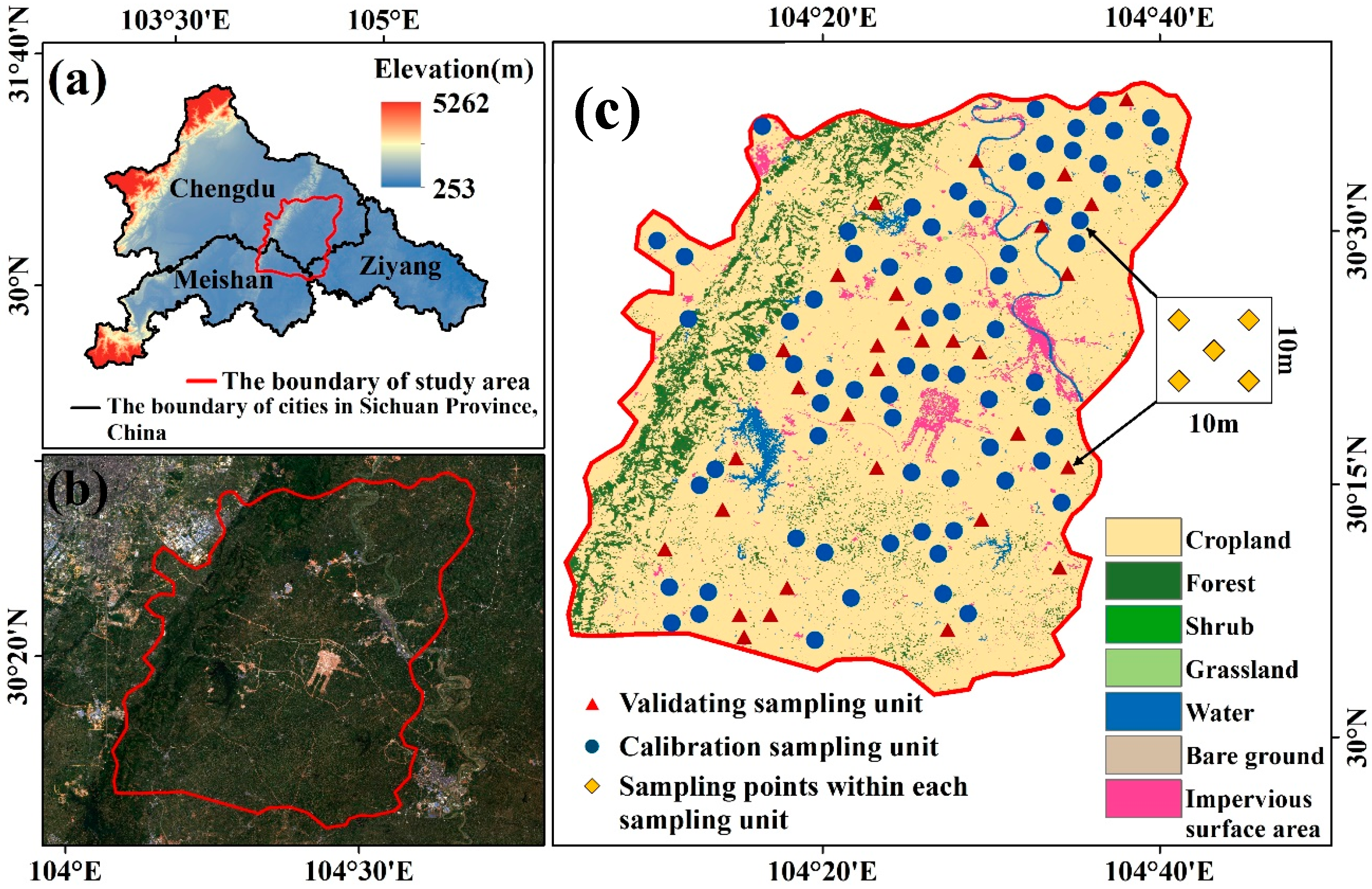
The study area is an agricultural zone in the Jianyang District (30°28′–30°42′ N, 104°15′–104°32′ E), located in the eastern Longquan Mountain in Chengdu, China. Its elevation ranges from 359 to 1017 m, which directly controls local water flow and soil movement (Figure 1). The climate is subtropical humid monsoon, with 900–1000 mm of annual rainfall and an average air temperature of 16.5 °C. Heavy summer rain helps move soil elements downward. The main soils are paddy soils (Stagnic Anthrosols) from Quaternary alluvium and purple soils (Cambisols) from Mesozoic rocks. These parent rocks mainly determine the natural background and spatial distribution of soil HMs.

2.2. Data Source and Description

2.2.1. Sample Collection and Analysis

In alignment with the Soil Environmental Quality Risk Control Standard for Agricultural Land (GB 15618-2018) [40], six critical soil HMs—As, Cd, Cu, Hg, Cr, and Pb—were selected for spatial modeling. Sampling collection was conducted on 11 August 2019, yielding 70 topsoil samples (0–20 cm) from regional farmlands (Figure 1c). For each sampling unit, a quadrat of at least 10 m × 10 m was delineated. A sampling unit was generated for five distinct sampling points. This involved collecting sub-samples from the geometric center and four equidistant diagonal locations, which were then mixed to ensure uniform spatial representation. The soil samples were transferred to the laboratory starting on 20 August 2019, where they were naturally air-dried, pulverized, and sifted through a 100-mesh polyethylene screen. Prior to chemical extraction, these prepared fractions were preserved in a desiccator to prevent moisture reabsorption.

For HM quantification, the pretreated soil samples were digested in polytetrafluoroethylene beakers using a sequential HNO₃–HClO₄–HF method [41]. Briefly, samples were first heated with 15 mL concentrated HNO₃ at 120 °C to near dryness. Then, 10 mL of the HNO₃-HClO₄ mixture (1:4, v/v) was added and heated at 150 °C. To dissolve the silicate lattice, 5 mL HF and 2 mL HClO₄ were subsequently introduced at 180 °C until the residue turned nearly white. Finally, the cooled residues were redissolved in 10% HNO₃ and diluted to 50 mL with ultrapure water. Ultimately, the elemental concentrations of the targeted HMs in the digested soil solutions were determined employing inductively coupled plasma mass spectrometry (ICP-MS; Thermo iCAP Q, Thermo Fisher Scientific, Waltham, MA, USA) [42]. The operating conditions of the ICP-MS were configured as follows: RF power at 1550 W, cooling gas flow at 14.0 L/min, auxiliary gas flow at 0.8 L/min, and nebulizer gas flow at 1.0 L/min. Stringent quality assurance and quality control (QA/QC) protocols were maintained throughout the analytical process of soil HMs. Reagent blanks (acid without soil), analytical duplicates, and national certified reference materials (GBW07425, National Research Center for Certified Reference Materials, China) were processed simultaneously with the field samples. A parallel sample was set for every 10 samples analyzed. The relative standard deviation for the duplicate samples was strictly controlled below 5%. All measured values fell completely within the certified calibration ranges of the reference materials, yielding analytical recovery rates between 93.7% and 104.5%, thereby confirming the high precision and accuracy of the utilized analytical method.

Table 1. Summary statistics of soil heavy metal concentrations in farmland.

Element	Mean Value (mg/kg)	Minimum Value (mg/kg)	Maximum Value (mg/kg)	Standard Deviation	The Coefficient of Variation (%)
As 1	4.65	1.07	12.11	2.51	53.98
Cd 2	0.43	0.15	0.83	0.20	46.51
Cu 3	32.70	9.87	58.44	14.52	44.40
Hg 4	0.26	0.05	0.52	0.11	42.31
Cr 5	62.56	23.66	105.66	17.65	28.21
Pb 6	29.03	14.36	56.63	10.05	34.62

¹ Arsenic; ² Cadmium; ³ Copper; ⁴ Mercury; ⁵ Chromium; ⁶ Lead.

summarizes the descriptive statistics of HM concentrations across the 70 topsoil samples.

2.2.2. Climate Data

All datasets (

Table 2. Description of the data used in this study.

Data Type	Datasets	Data Name	Unit	Spatial Resolution	Source	Data Availability
Soil samples data	/	As 7	mg/kg	/	/	Sample collection and analysis
		Cd 8
		Cu 9
		Hg 10
		Cr 11
		Pb 12
Climate data	China-1km-Climatology 1	TEM 13	°C	1 km	Peng et al. [43]	https://data.tpdc.ac.cn/ (accessed on 1 August 2025)
		PRE 14	mm	1 km
	HiMeteo-China 2	RH 15	%	1 km	Zhao et al. [44]
Topographical data	SRTM 3	DEM 16	m	30 m	EROS 23	https://earthexplorer.usgs.gov/ (accessed on 5 August 2025)
PM2.5 concentration data	China High PM2.5 4	PM2.5 17	µg/m3	1 km	Wei et al. [45]	https://data.tpdc.ac.cn/ (accessed on 7 August 2025)
Remote sensing data	Landsat 8 5	/	/	30 m	CNIC 24	https://www.gscloud.cn/ (accessed on 8 August 2025)
Soil physicochemical properties data	HWSD 2.0 6	pH	/	1 km	FAO 25	https://www.fao.org/home/en/ (accessed on 15 August 2025)
		CEC 18	meq/100 g
		AP 19	mg/kg
		SC 20	%
		CC 21	%
		SOM 22	%

¹ 1 km monthly temperature and precipitation dataset for China; ² 1 km daily high-accuracy meteorological dataset for China; ³ Shuttle Radar Topography Mission; ⁴ ChinaHighAirPollution (CHAP) PM_2.5 dataset; ⁵ Landsat 8 OLI/TIRS Collection 2 Level-2 Science Products; ⁶ Harmonized World Soil Database; ⁷ Arsenic; ⁸ Cadmium; ⁹ Copper; ¹⁰ Mercury; ¹¹ Chromium; ¹² Lead; ¹³ air temperature; ¹⁴ precipitation; ¹⁵ relative humidity; ¹⁶ digital elevation model; ¹⁷ particulate matter; ¹⁸ cation exchange capacity; ¹⁹ available phosphorus; ²⁰ sand content; ²¹ clay content; ²² soil organic matter; ²³ Earth Resources Observation and Science Center; ²⁴ the Computer Network Information Center Chinese Academy of Sciences; ²⁵ the Food and Agriculture Organization of the United Nations.

) that include climate data, topographical data, PM_2.5 concentration data, remote sensing data, and soil physicochemical properties data underwent geometric correction and registration. The coordinates were consistently reprojected to the WGS 84/UTM Zone 49 N system and clipped to align with the extent of the study area. Gridded climate datasets with a 1 km spatial resolution were used in this study. It specifically encompasses precipitation, temperature, and relative humidity, which were downloaded from the National Tibetan Plateau Data Center (https://data.tpdc.ac.cn/) (Table 2).

2.2.3. Topographical Data

To calculate essential terrain parameters—specifically, slope and aspect—this study relied on a 30 m resolution digital elevation model (DEM). As detailed in Table 2, this base topographic data was derived from the Shuttle Radar Topography Mission (SRTM) and obtained via the United States Geological Survey portal.

2.2.4. PM_2.5 Concentration Data

This research utilized spatial PM_2.5 records (1 km resolution) supplied by the National Tibetan Plateau Data Center (Table 2). As assessed by Wei et al. [45], this dataset demonstrates excellent reliability, yielding an R² of 0.92 and an RMSE of 10.76 µg/m³.

2.2.5. Remote Sensing Data

The remote sensing data were atmospherically corrected using the Fast Line-of-sight Atmospheric Analysis of Spectral Hypercubes model. A cloud-free Landsat 8 image, acquired on 11 August 2019, was acquired from the Geospatial Data Cloud (Table 2). Surface reflectance bands spanning the visible (blue, green, red), near-infrared (NIR), and short-wave infrared (SWIR) bands, in conjunction with the thermal infrared band, were utilized to derive land surface temperature (LST) and vegetation indices (

Table 3. The environmental variables derived from the digital elevation model (DEM) and the Landsat 8 image.

Environment Variables	Data	Abbreviation	Definition or Formula
Topographic variables	Elevation	/	Vertical distance from mean sea level
	Aspect	ASP	Topographic facing orientation
	Slope	SLO	Topographic surface inclination
Land surface temperature	Land surface temperature	LST [46]	The mono-window algorithm
Landsat reflectance band	band 2	B2	Reflectance value of the blue band
	band 3	B3	Reflectance value of the green band
	Band 4	B4	Reflectance value of the red band
	Band 5	B5	Reflectance value of the near-infrared band
	Band 6	B6	Reflectance value of the short-wave infrared 1 band
	Band 7	B7	Reflectance value of the short-wave infrared 2 band
Vegetation indices	Normalized difference vegetation index	NDVI [47]	$\mathrm{NDVI}={\displaystyle \frac{\mathrm{B}5- \mathrm{B}4}{\mathrm{B}4+\mathrm{B}5}}$
	Enhanced vegetation index	EVI [48]	$\mathrm{EVI}={\displaystyle \frac{2.5 (\mathrm{B}5 - \mathrm{B}4)}{\left(\mathrm{B}5+6\mathrm{B}4 - 7.5\mathrm{B}2\right)+1}}$
	Mid-infrared vegetation index	MVI [49]	$\mathrm{MVI}={\displaystyle \frac{\mathrm{B}5}{\mathrm{B}6}}$
	Soil-adjusted vegetation index	SAVI [50]	$\mathrm{SAVI}={\displaystyle \frac{1.5 (\mathrm{B}5 - \mathrm{B}4)}{\mathrm{B}5+\mathrm{B}4+0.5}}$
	Soil-adjusted total vegetation index	SATVI [51]	$\mathrm{SATVI}={\displaystyle \frac{2 (\mathrm{B}6 - \mathrm{B}4)}{\mathrm{B}6+\mathrm{B}4+1}} - {\displaystyle \frac{\mathrm{B}7}{2}}$

).

2.2.6. Soil Physicochemical Properties Data

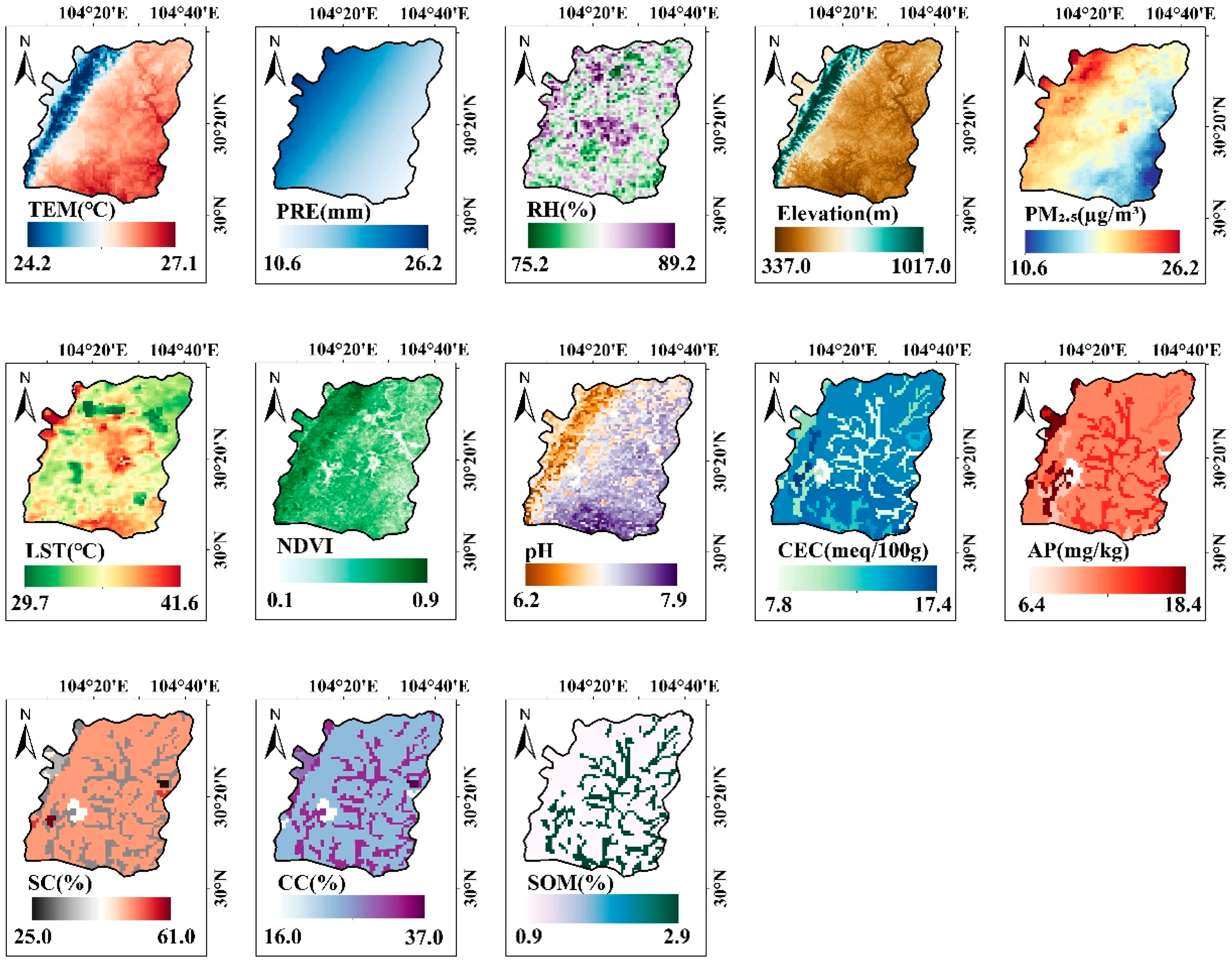
Soil physicochemical properties data were obtained from the Harmonized World Soil Database version 2.0 (HWSD v2.0), mainly developed by the Food and Agriculture Organization of the United Nations (Table 2). HWSD v2.0 provides globally consistent soil raster layers at a 1 km spatial resolution. In this study, pH, cation exchange capacity (CEC), available phosphorus (AP), sand content (SC), clay content (CC), and soil organic matter (SOM) were selected as the potential driving factors. The spatial distribution of all potential driving factors associated with HM contamination in the investigated agricultural soils is presented in Figure 2.

2.3. Methodology

2.3.1. HASM

HASM is grounded in the fundamental theorem of surfaces from differential geometry [52] and has been successfully applied across diverse domains [53,54]. Theoretically, a surface is uniquely determined by the coefficients of its first and second fundamental forms. By discretizing the partial differential equations derived from the Gaussian fundamental equations, the governing equations of HASM can be formulated as a linear system. To enhance numerical stability and facilitate computation, the HASM formulation is expressed in matrix-vector notation. If a soil HM surface can be expressed as U = f(x,y), then the HASM expression is given as follows:

$$\left\{\begin{array}{c}{\min ‖\left[\begin{array}{c}{\Phi }_1\\ {\Phi }_2\\ {\Phi }_3\end{array}\right] \times {\mathrm{U}}^{\mathrm{k}+1} - \left[\begin{array}{c}{\mathrm{h}}_1^{\mathrm{k}}\\ {\mathrm{h}}_2^{\mathrm{k}}\\ {\mathrm{h}}_3^{\mathrm{k}}\end{array}\right]‖}_2\\ \mathrm{s}.\mathrm{t}.\Psi \times {\mathrm{U}}^{\mathrm{k}+1} = {\mathrm{y}}_{\mathrm{obs}}\end{array}\right.$$

(1)

where U^k+1 is the (n + 1)–th iteration of the HM surface U. ${\Phi }_1$, ${\Phi }_2$, and ${\Phi }_3$ are the sparse coefficient matrices derived from the finite difference approximations of the first, second, and third Gaussian equations, respectively. ${\mathrm{h}}_1^{\mathrm{k}}$, ${\mathrm{h}}_2^{\mathrm{k}}$, and ${\mathrm{h}}_3^{\mathrm{k}}$ represent the right-hand side vectors updated at the k-th iteration, containing information from the previous step. Ψ is the sampling matrix that maps the grid nodes to the locations of the sampling points. y_obs is the vector of measured HM content values at the sampling locations.

2.3.2. Downscaling Methodology

Machine learning is an effective data-driven approach for identifying complex relationships between predictors and target variables and for improving predictive performance in spatial modeling [55]. In this study, four machine learning methods, including ANNs [56], SVMs [57], RF [58], and XGBoost [59], were introduced to analyze the relationships between soil HM concentrations and environmental variables, including topographic variables, LST, Landsat reflectance band, and vegetation index (Table 3). These machine learning models were applied to downscale low spatial resolution soil HM data to high spatial resolution soil HM data.

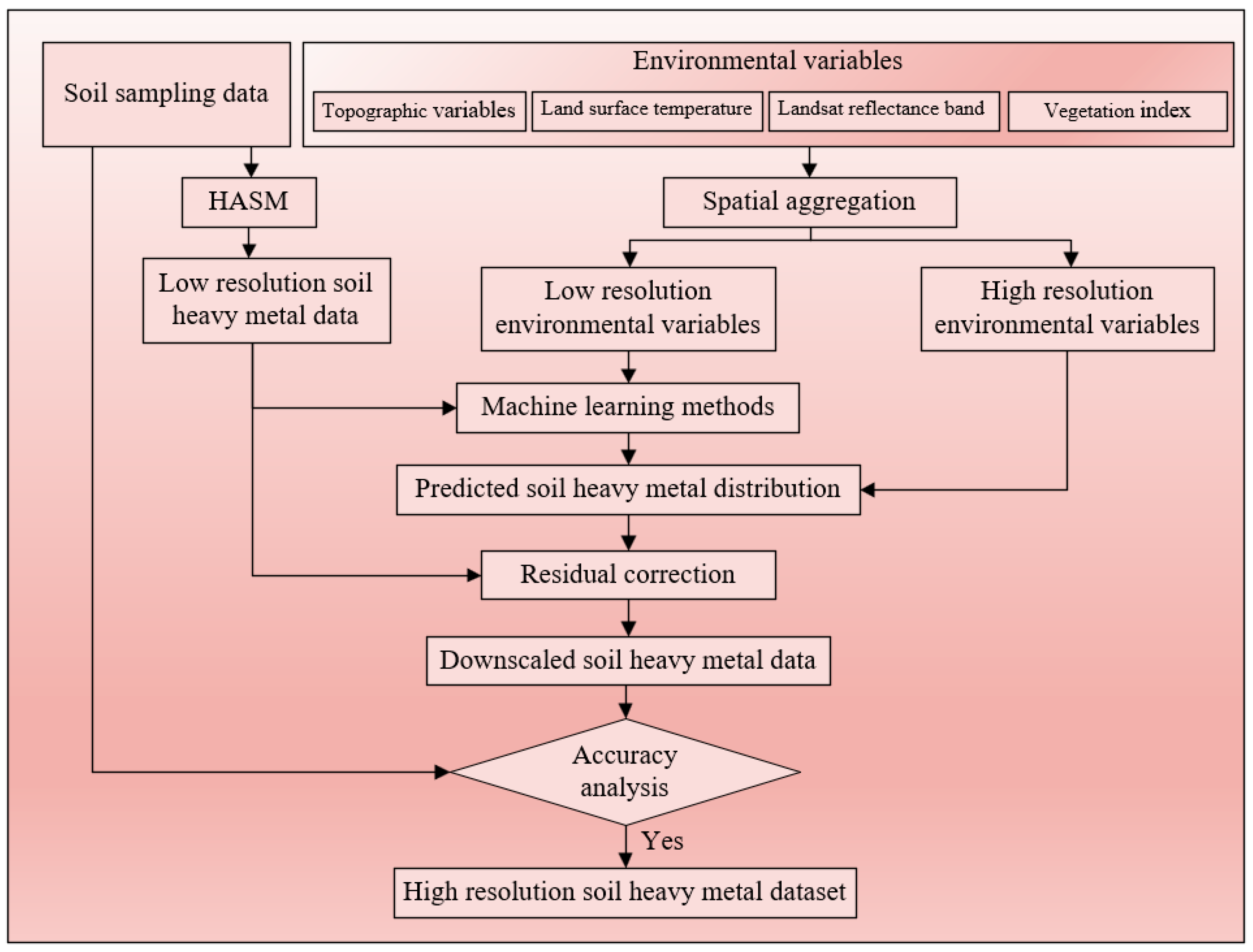
The specific workflow of soil HM downscaling used in this study is illustrated in Figure 3. Based on the HASM framework, interpolation was first performed on the soil sampling data to generate low spatial resolution soil HM data, while environmental variables were aggregated to low and high spatial resolutions. A machine learning model was then used to establish the scale conversion relationship between low spatial resolution soil HM concentrations and environmental variables at the low spatial resolution, as expressed in Equation (2). The residual at the low resolution was calculated according to Equation (3). Assuming that the established relationship remains valid across spatial scales, it was transferred to the high spatial resolution, and the interpolated residual was added to obtain the downscaled soil HM concentration, as shown in Equation (4). Thus, high spatial resolution soil HM data were generated.

$${HM}_{1000}=f({ELE}_{1000},{ASP}_{1000},{SLO}_{1000},{LST}_{1000},{NDVI}_{1000},{EVI}_{1000},{MVI}_{1000},{SAVI}_{1000},{SATVI}_{1000})$$

(2)

$$∆{HM}_s={HM}_s-\overline{{HM}_s}$$

(3)

$${HM}_{100}=f\left({ELE}_{100},{ASP}_{100},{SLO}_{100},{LST}_{100},{NDVI}_{100},{EVI}_{100},{MVI}_{100},{SAVI}_{100},{SATVI}_{100}\right)+∆{HM}_s$$

(4)

where $H{M}_{1000}$ represents the estimated soil HM concentration at the 1000 m spatial resolution; $EL{E}_{1000}$, $AS{P}_{1000}$, $SL{O}_{1000}$, $LS{T}_{1000}$, $NDV{I}_{1000}$, $EV{I}_{1000}$, $MV{I}_{1000}$, $SAV{I}_{1000}$, and $SATV{I}_{1000}$ denote the elevation, aspect, slope, land surface temperature, normalized difference vegetation index, enhanced vegetation index, mid-infrared vegetation index, soil-adjusted vegetation index, and soil-adjusted total vegetation index, respectively, aggregated to the 1000 m spatial resolution; $\Delta H{M}_{s }$ represents the residual at the 1000 m resolution; $H{M}_s$ and ${\overline{HM}}_s$ refer to the soil HM concentration generated by the HASM model and the estimated value produced by the machine learning model at the 1000 m spatial resolution, respectively; $H{M}_{100}$ represents the downscaled soil HM concentration at the 100 m spatial resolution; $EL{E}_{100}$, $AS{P}_{100}$, $SL{O}_{100}$, $LS{T}_{100}$, $NDV{I}_{100}$, $EV{I}_{100}$, $MV{I}_{100}$, $SAV{I}_{100}$, and $SATV{I}_{100}$ denote the environmental variables aggregated to the 100 m spatial resolution.

In this study, a spatial resolution of 1000 m was used as the low spatial resolution because the soil HM concentrations were generated at 1 km resolution using the HASM method. Accordingly, the original 30 m DEM, slope, aspect, Landsat bands, LST, NDVI, EVI, MVI, SAVI, and SATVI were resampled to 1 km and 100 m using bilinear interpolation in ArcGIS 10.8. The 100 m resolution, rather than the original 30 m resolution, was selected as the high spatial resolution because previous downscaling studies have shown that the ratio between high and low spatial resolutions should generally remain within a reasonable range, preferably not exceeding approximately 10 times [60]. Otherwise, an excessively large resolution gap may lead to scale-effect distortion [61]. Nevertheless, information loss during resampling is unavoidable because when multiple high-resolution pixels are combined into a low-resolution pixel, fine-scale details are averaged and smoothed [62].

All machine learning downscaling models were implemented in the R environment (version 4.3.2): ANNs, as nonlinear algorithms, are suitable for downscaling because they can represent complex relationships between target variables and environmental predictors [63]. ANNs generally consist of an input layer, one or more hidden layers, and an output layer, in which neurons are connected through weights and bias or threshold terms to establish nonlinear input–output results [64]. For the ANN model, implementation was performed with the NeuralNet package (version 1.44.2). The predictive performance of an ANN is mainly governed by several key parameters, including the number of nodes in the hidden layer, learning function, learning rate, momentum coefficient, and training epochs. During the training process, the learning rule iteratively adjusts the connection weights and thresholds based on the error between the observed and predicted outputs, and 10-fold cross-validation is used to enhance model robustness and predictive accuracy.

SVMs, rooted in statistical learning theory, are suitable for downscaling because they can characterize nonlinear relationships in data and handle high-dimensional pattern recognition tasks [65]. In this study, the SVM model was used with the LIBSVM package (version 3.37), and three commonly used kernel functions, namely radial basis function, polynomial, and linear, were tested [66]. To improve SVM performance, 10-fold cross-validation was conducted for each kernel function, and the final parameter setting was chosen from different combinations of penalty coefficient (C) and gamma (γ) according to the lowest model error.

RF is an ensemble learning method suitable for downscaling, in which a large number of random and uncorrelated decision trees are used to characterize nonlinear relationships and complex interactions among environmental predictors [67]. The RF model is developed by constructing multiple decision trees from bootstrap resampled datasets and randomly selected feature subsets, while the final prediction is derived from the aggregated outputs of all trees [68]. The RF model was employed using the “randomForest” package (version 4.7-1.2). The predictive performance of RF was mainly governed by two key parameters, namely ntree, the number of decision trees, and mtry, the number of predictor variables considered at each split. In this study, 10-fold cross-validation was used to determine the optimal values of ntree and mtry by minimizing model error.

Built upon classification and regression trees, XGBoost can address various machine learning tasks by improving the traditional gradient boosting decision tree framework and enhancing the representation of nonlinear relationships and complex interactions among environmental predictors [69]. Built upon gradient boosting theory, XGBoost develops an additive model by sequentially fitting decision trees to the residuals produced by preceding learners [70]. In this study, the XGBoost model was implemented using the “XGBoost” package (version 3.2.1.1) and the “Matrix” package. Parameter tuning for XGBoost was performed under a 10-fold cross-validation framework, where the max_depth, the n_estimators, gamma, the learning_rate, the subsample, and the colsample_bytree were jointly assessed, and the optimal combination was selected on the basis of the lowest model error.

2.3.3. Model Evaluation Metrics

Soil HM concentration for training and validation samples was extracted using the Extract Values to Points tool in ArcGIS 10.8. To validate the accuracy of the predicted soil HM concentration results based on the different HASM–machine learning-based downscaling approach, two standard statistical indicators were employed: R² and the RMSE [71,72]. The calculation formulas for these metrics are expressed as follows:

$${\mathrm{R}}^2 = 1 - {\displaystyle \frac{{\displaystyle {\sum }_{\mathrm{i}=1}^n}{\left({\mathrm{y}}_i - \widehat{{\mathrm{y}}_i}\right)}^2}{{\displaystyle {\sum }_{i=1}^n}{\left({\mathrm{y}}_i - \stackrel{\mathrm{-}}{\mathrm{y}}\right)}^2}}$$

(5)

$$\mathrm{RMSE}=\sqrt{{\displaystyle \frac{1}{n}}{\displaystyle {\sum }_{i=1}^n}{\left({\mathrm{y}}_i - \widehat{{\mathrm{y}}_i}\right)}^2}$$

(6)

where n denotes the number of soil samples in the validation set; y_i represents the measured HM concentration of the i-th sample; ${\widehat{\mathrm{y}}}_i$ is the corresponding predicted value generated by the HASM–machine downscaling approach; and $\overline{\mathrm{y}}$ is the mean of the measured values.

2.3.4. Geographical Detector Model

The geographical detector (GD) model is a spatial statistical method used to quantitatively assess spatial stratified heterogeneity and identify driving factors by measuring the spatial correlation between variables [73]. This study employed the factor detector and interaction detector modules using the Geodetector package (version 1.0-5) in the R language. Specifically, the q was employed to investigate the primary driving factors and their interactive effects on soil HMs in the study area. The governing equation of the factor detector is expressed as follows [74]:

$$\mathrm{q}=1 - {\displaystyle \frac{{\displaystyle {\sum }_{\mathrm{h}=1}^{\mathrm{L}}}{\mathrm{N}}_{\mathrm{h}}{\mathrm{\sigma }}_{\mathrm{h}}^2}{\mathrm{N}{\mathrm{\sigma }}^2}}$$

(7)

where h = 1, …, L represents the classes of the explanatory variable X; N_h and N denote the number of sample units in stratum h and the entire study region, respectively; ${\mathrm{\sigma }}_{\mathrm{h}}^2$ and ${\mathrm{\sigma }}^2$ correspond to the variance of the pollutant concentration within stratum h and the global variance. The value of q ∈ [0, 1] indicates the degree to which the driving factors explain the spatial variation in soil HMs. The interaction detector assesses the combined influence of paired explanatory factors on the spatial distribution of soil HMs (

Table 4. Categorization of the interactive effects between pairs of driving factors.

Number	Interaction Type	Judgment Criteria
1	Non-linear weakening	q(X1 ∩ X2) < Min(q(X1),q(X2))
2	Single-factor non-linear attenuation	Min(q(X1),q(X2)) < q(X1 ∩ X2) < Max(q(X1),q(X2))
3	Two-factor enhancement	q(X1 ∩ X2) > Max(q(X1),q(X2))
4	Mutal independence	q(X1 ∩ X2) = q(X1) + q(X2)
5	Non-linear enhancement	q(X1 ∩ X2) > q(X1) + q(X2)

).

2.3.5. Multiscale Geographically Weighted Regression Model

Multiscale geographically weighted regression (MGWR) is a local spatial regression method that deals with spatially nonstationary relationships and allows different explanatory variables to operate at varying spatial scales by using different bandwidths [75]. This study applies the MGWR model (software version 2.2.1) to reveal the extent to which dominant driving factors influence the spatial patterns and trends of soil HMs in the study area. The MGWR model is generally formulated as [76]:

$$y_i = {\mathrm{\beta }}_{\mathrm{b}\mathrm{\omega }0}\left(u_i,v_i\right) + {\displaystyle {\sum }_{j=1}^k}{\mathrm{\beta }}_{\mathrm{b}\mathrm{\omega }\mathrm{j}}\left(u_i,v_i\right){\mathrm{x}}_{i\mathrm{j}} +{ \mathrm{\epsilon }}_i$$

(8)

where y_i denotes the dependent variable at location i with coordinates (u_i, v_i); β_bω0 is the intercept specific to bandwidth bω0; k represents the number of explanatory variables; and β_bωj signifies the local regression coefficient for the j-th predictor variable x_ij, estimated using a unique optimized bandwidth bωj; and ε_i represents the random error term at location i. Parameter estimation typically employs an iterative back-fitting algorithm integrated with adaptive spatial kernel functions to weight neighboring observations based on proximity.

3. Results and Discussion

3.1. Assessment of the HASM–Machine Learning Methods

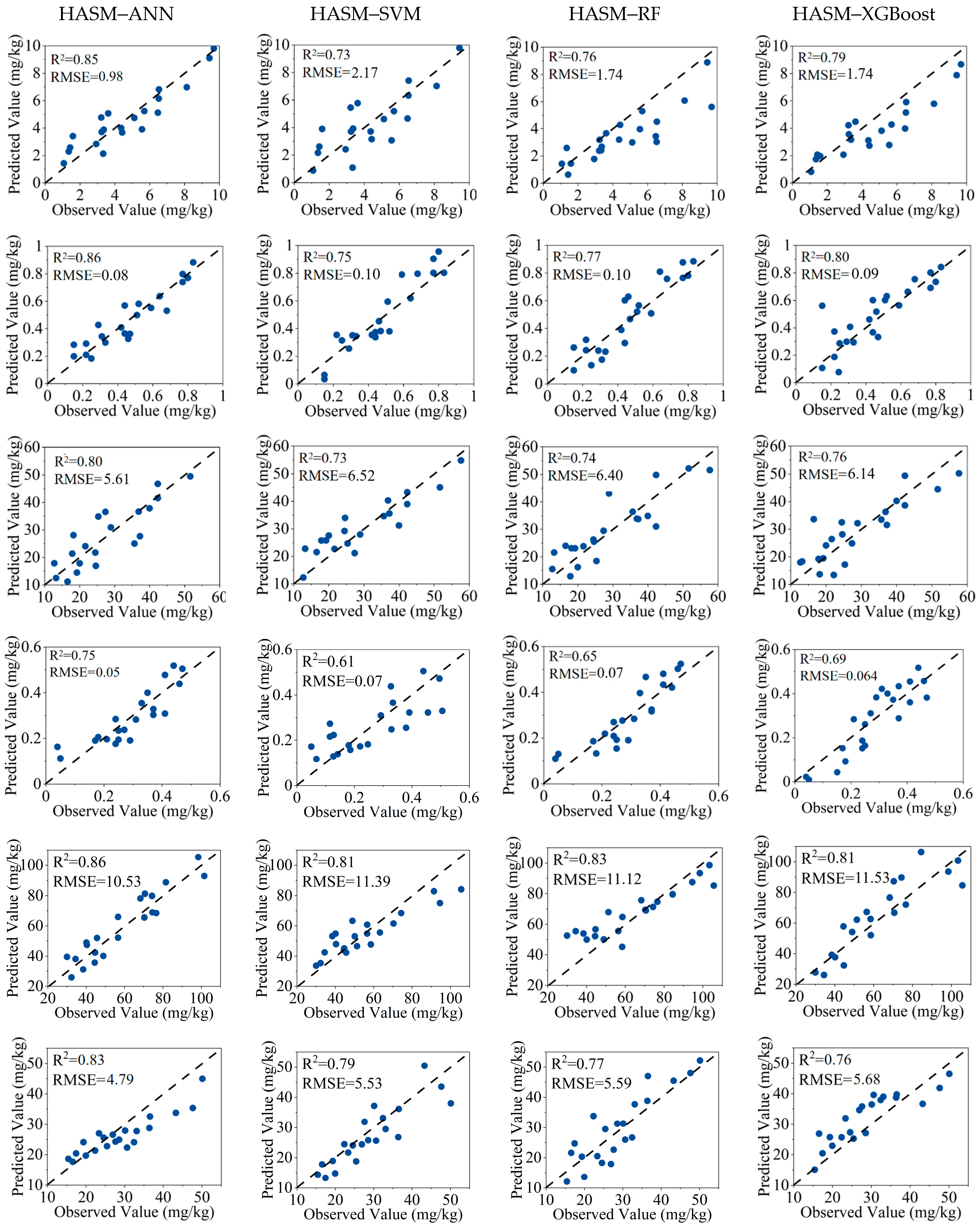
To evaluate the predictive accuracy of four HASM–machine learning methods (HASM–ANN, HASM–SVM, HASM–RF, and HASM–XGBoost), the soil HM samples were randomly partitioned into two independent subsets. Specifically, 70% of the observed sample points (n = 49) were utilized to train the hybrid methods, while the remaining 30% (n = 21) were withheld for validation. Method robustness was subsequently quantified using the R² and RMSE. For all machine learning methods, parameter tuning was performed based on 10-fold cross-validation to determine the optimal parameter combination. In this study, the optimal hyperparameter settings are described in

Table 5. Optimal hyperparameter settings of machine learning models in this study.

Model	Hyperparameter	As 1	Cd 2	Cu 3	Hg 4	Cr 5	Pb 6
ANN	number of nodes	4	5	2	3	4	3
	learning rate	0.03	0.04	0.01	0.02	0.03	0.02
	momentum coefficient	0.7	0.8	0.7	0.7	0.8	0.7
	training epoch	100	200	100	100	200	100
SVM	penalty coefficient (C)	4	6	7	5	7	4
	gamma (γ)	0.1	0.1	0.2	0.1	0.2	0.1
RF	mtry	9	8	8	8	9	9
	ntree	200	300	200	200	300	200
XGBoost	max_depth	7	7	9	8	8	9
	n_estimators	300	500	400	300	400	500
	gamma	0.1	0.1	0.1	0	0.1	0.1
	learning_rate	0.01	0.05	0.1	0.07	0.06	0.09
	subsample	0.8	0.8	0.9	0.9	0.8	0.8
	colsample_bytree	0.6	0.7	0.6	0.7	0.7	0.6

¹ Arsenic; ² Cadmium; ³ Copper; ⁴ Mercury; ⁵ Chromium; ⁶ Lead.

.

As illustrated in Figure 4, the predictive results for the six soil HMs (As, Cd, Cu, Hg, Cr, and Pb) varied, with R² values spanning 0.73–0.85, 0.75–0.86, 0.73–0.80, 0.61–0.75, 0.81–0.86, and 0.76–0.83, alongside RMSE values of 0.98–2.17 mg/kg, 0.08–0.10 mg/kg, 5.61–6.52 mg/kg, 0.05–0.07 mg/kg, 10.53–11.53 mg/kg, and 4.79–5.68 mg/kg, respectively. These metrics clearly demonstrate that the HASM–ANN provides superior predictive accuracy with the lowest error rates among the four tested methods. This superior performance is primarily attributed to the model’s capacity to account for spatial non-stationarity, thereby dynamically capturing the spatially varying relationships between soil HMs and environmental variables. Consequently, the HASM–ANN framework proves highly adept at resolving complex spatial heterogeneity.

Although machine learning models have been extensively utilized in the spatial downscaling of soil HMs, some methods may exhibit certain limitations when handling highly heterogeneous spatial data [77]. Algorithms like SVMs can be sensitive to localized noise and hyperparameter configurations [78]. RF models, despite their robust nonlinear modeling capabilities, might encounter challenges in extrapolating extreme values beyond the training data range, which could affect the identification of high-pollution hotspots [79]. Additionally, XGBoost models sometimes yield step-like spatial surfaces that may not perfectly reflect the natural continuity of soil elements, and intricate parameter tuning can pose overfitting risks under limited sample sizes [80].

An ANN possesses strong nonlinear mapping and self-learning capabilities, enabling it to characterize the complex nonlinear relationships between low spatial resolution soil heavy metal concentrations and multi-source environmental variables without presupposing a specific functional form [81,82]. Therefore, an ANN is well-suited for spatial downscaling in this study. Previous studies have shown that ANNs have been widely applied in statistical and spatial downscaling, and can effectively establish scale conversion relationships between low-resolution target variables and high spatial resolution auxiliary factors [83,84]. Compared with traditional linear models, ANNs can more effectively integrate multi-source auxiliary variables, including topographic, remote sensing, climate, and soil physicochemical factors, thereby improving the representation of spatial heterogeneity and the predictive accuracy of high spatial resolution results.

3.2. Spatial Distribution Characteristics of Soil HMs

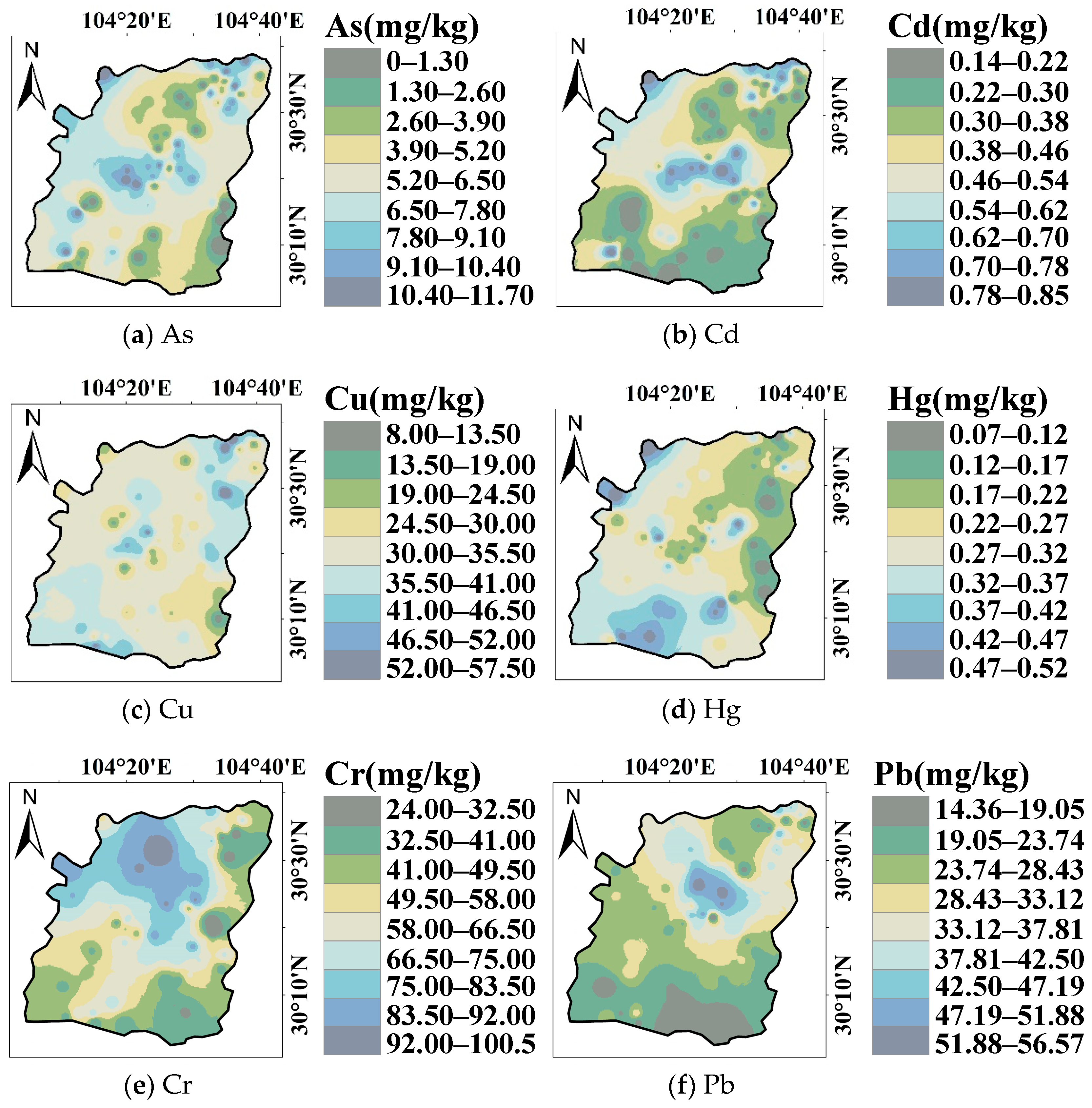
Figure 5 illustrates the spatial distribution characteristics of the soil HMs based on the HASM–ANN in the study area. As shown in Figure 5a, the high-concentration areas of As are primarily distributed in the midwestern region. These areas are specifically concentrated across Tong’an Town, Luodai Town, and Shanquan Town. In addition, significantly high-concentration clusters of As are located in the northeastern part of the study area. These include Zhaojia Town, Sanxi Town, and Gaoban Town. Furthermore, a localized high-concentration cluster is observed around Danjing Town in the south. Similarly, Cd displays a distinct “central aggregation” pattern (Figure 5b), with high-concentration clusters notably distributed in the midwestern region of the study area. Within these areas, Cd concentrations reach 0.70 to 0.85 mg/kg. By contrast, Cu exhibits a fragmented distribution (Figure 5c), with high-concentration clusters sporadically distributed across the northeastern, central, and southern regions of the study area. Specifically, the northeastern high-concentration clusters are located in Gaoban Town, Sanxi Town, and Zhaojia Town. Sporadic high-concentration clusters in the central region are distributed near Tong’an Town and Shanquan Town. Additionally, a localized high-concentration cluster is observed at the junction of Danjing Town and Sancha Town in the south. Concurrently, significantly low concentration clusters exist in scattered central areas and the southeastern region. These primarily include the surroundings of Baihe Town and Xihe Town, as well as the vicinity of Lujia Town in the southeast. Finally, Hg forms distinct high-concentration clusters in both the southern and northwestern sectors of the study area (Figure 5d). Its highest concentration reaches 0.52 mg/kg. The southern high-concentration clusters are distinctly located in Danjing Town, Sancha Town, and Lujia Town. Meanwhile, a significant northwestern high-concentration cluster is situated around Qingquan Town and Renhe Town. Similarly, the high-concentration areas of Cr are primarily distributed in the northwestern region (Figure 5e). These areas are specifically concentrated across Qingquan Town and Renhe Town. Its highest concentration reaches 100.50 mg/kg. Concurrently, significantly low concentration clusters exist in scattered southern and southeastern regions. Furthermore, Pb exhibits a fragmented distribution (Figure 5f), with high-concentration clusters sporadically distributed across the central and northeastern regions of the study area. A localized high-concentration cluster is observed around Baiguo Town and Wufeng Town in the central region. Within these areas, high Pb concentrations reach 51.88 to 56.57 mg/kg. In addition, significantly high-concentration clusters of Pb are located in the northeastern part of the study area. These include Zhaojia Town and Sanxi Town.

3.3. The Influence of Driving Factors on Soil HM Contamination

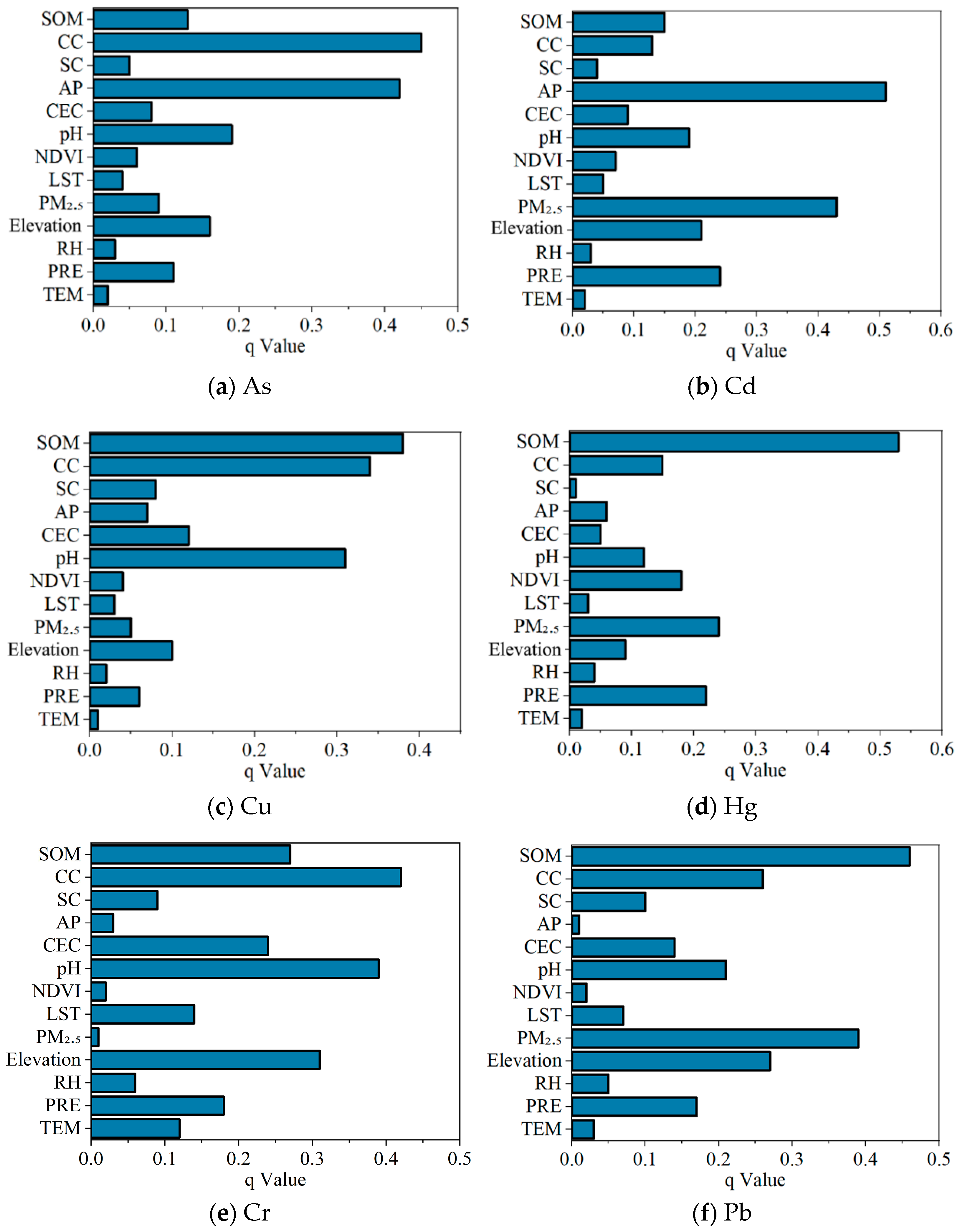
Continuous explanatory variables were discretized before GD analysis. Following Jiang et al. [85], several discretization methods, including natural breaks and quantile breaks, were tested with the number of strata ranging from three to eight. The optimal parameter combination was selected according to the maximum q-statistic, and the natural breaks classification method with six strata was ultimately adopted because it provided better stratification and stronger explanatory power. As shown in Figure 6, the 13 driving factors exerted varying impacts on the soil HMs in the study area. Specifically, the dominant driving factors for As were CC (q = 0.45) and AP (q = 0.42); Cd was highly driven by AP (q = 0.51) and PM_2.5 (q = 0.43). Additionally, Cu was mainly influenced by SOM (q = 0.38), CC (q = 0.34), and pH (q = 0.31); and the driving factor with the highest explanatory power for Hg was SOM (q = 0.53). Furthermore, Cr was predominantly influenced by CC (q = 0.42), pH (q = 0.39), and elevation (q = 0.31); while the most significant driving factors for Pb were SOM (q = 0.46) and PM_2.5 (q = 0.39). The accumulation of As in the study area can be primarily attributed to the widespread distribution of purple soil. Specifically, the CC within this soil type is enriched with iron and aluminum oxides, which exhibit a strong affinity for As [86], thereby driving its continuous accumulation. Furthermore, agricultural land uses dominate the study area. Given that agricultural fertilizers inherently contain trace soil HM impurities, their sustained application likely co-introduces As alongside AP. This concurrent input consequently elevates the concentrations of both AP and As within the soil matrix [87,88].

Climatically, the region is characterized by a subtropical monsoon system, dominated by the southerly summer monsoon [89]. Cd bound to PM_2.5, originating from anthropogenic emissions in southern industrial municipalities, undergoes long-range transport via these monsoonal winds. Subsequent atmospheric deposition acts as a primary driver for the elevated soil Cd concentrations in the study area [90,91]. Conversely, CC in purple soils strongly binds with SOM to form stable complexes. This CC–SOM coupling significantly enhances the soil’s adsorption and retention capacity for Cu [92], thereby promoting its localized accumulation. Moreover, the weakly acidic environment (pH ≈ 6.3) in the western high altitude region facilitates Cu desorption and leaching. Driven by the topographic gradient, mobilized Cu migrates via surface runoff toward the eastern low-lying areas. Upon entering the weakly alkaline environment (pH ≈ 7.7) of the eastern sector, the transported Cu undergoes re-adsorption and immobilization. The synergistic interplay of these topographical and geochemical factors elucidates the elevated Cu concentrations observed in the east. Owing to its high volatility, gaseous Hg derived from anthropogenic emissions in southern cities, coupled with Hg vapor volatilized from adjacent soils [93], is similarly transported to the study area via monsoonal currents. Upon contact with the soil interface, these gaseous Hg species are readily sequestered by topsoil SOM [94], further exacerbating local Hg accumulation. Regarding Cr, its spatial distribution appears to be strongly governed by natural pedogenic processes. The considerable explanatory power of CC and pH suggests that Cr is primarily derived from the weathering of parent materials and is subsequently stabilized by clay minerals. Additionally, variations in elevation and pH likely regulate the local weathering intensity and the subsequent mobility of Cr within the soil profile [95]. For Pb, the substantial influence of SOM and PM_2.5 indicates a combination of anthropogenic input and geochemical retention. Pb emitted from industrial activities or vehicular exhaust is often transported via PM_2.5 and deposited into the soil [96]. Once deposited, Pb exhibits a strong affinity for SOM, forming stable complexes that restrict its downward leaching, thereby promoting its accumulation in the surface soil layers [97]. Moreover, elevation variations may further influence the atmospheric deposition patterns of these PM_2.5-bound Pb particles across the terrain. These explanations regarding soil properties are consistent with the findings of Marković et al. [98,99], who showed that they regulate metal distribution and speciation by controlling adsorption, mobility, and availability. Clay minerals retain metals through adsorption and ion exchange, pH governs metal solubility and precipitation, and SOM binds metals via organic complexation. Their study also supported the use of ANN-based approaches to interpret nonlinear soil metal relationships.

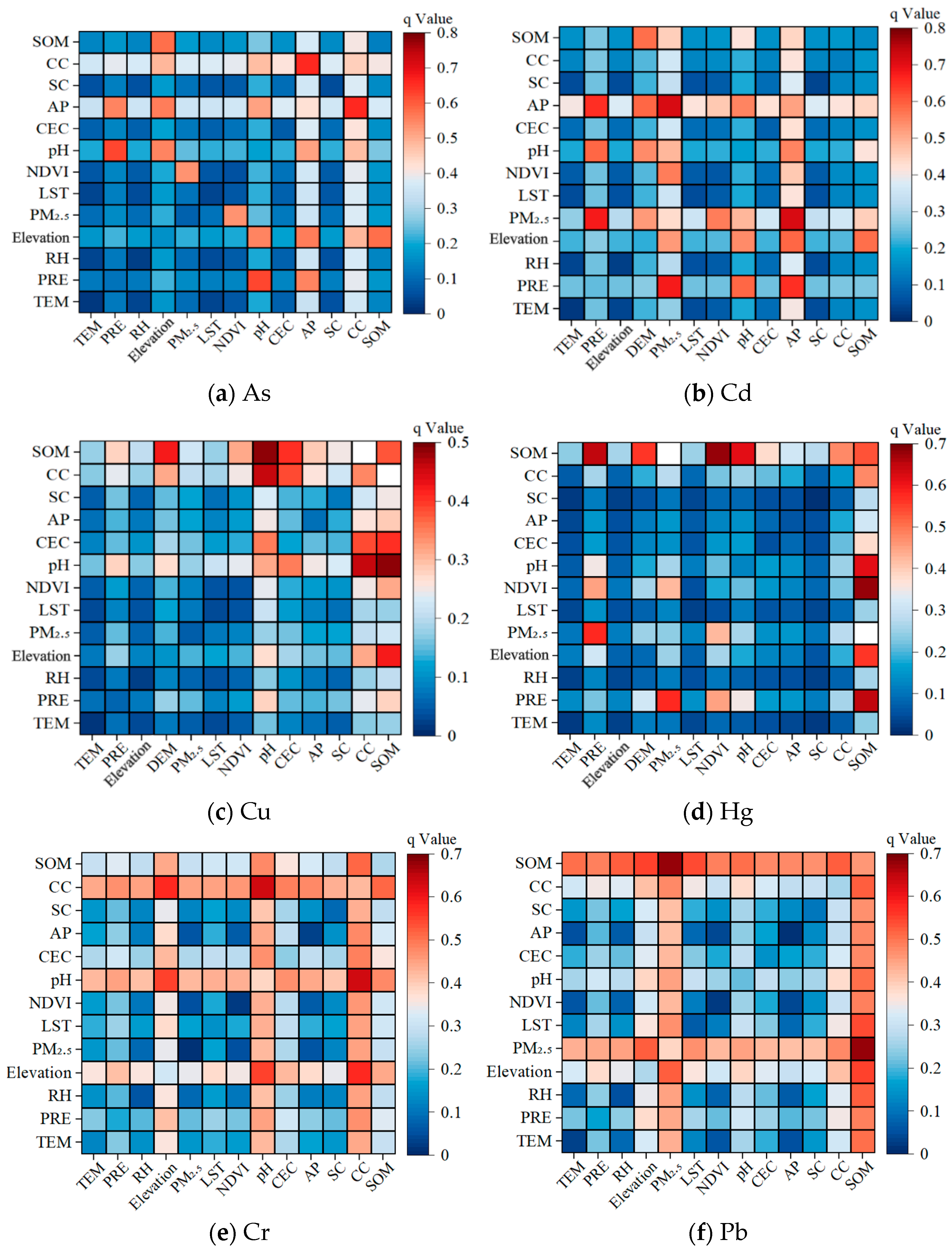
Figure 7 illustrates the results of the interaction detector for the study area. The interactions among the driving factors influencing soil HM concentrations were predominantly characterized by non-linear enhancement. Specifically, regarding As, the interaction between AP and CC (AP ∩ CC) yielded a substantial q-value of 0.66. This phenomenon is primarily ascribed to the robust adsorption capacity of CC within the purple soil for exogenous As [100]. Such pedological characteristics facilitate the sequestration of As derived from agrochemical fertilizers, thereby intensifying its spatial accumulation across the study region. This was followed by the interaction between AP and PRE, which reached a q-value of 0.62. It is postulated that PRE not only accelerates the dissolution and liberation of As from agricultural inputs but also promotes the lateral migration and convergence of the element in localized depressions via surface runoff, further elevating As concentrations in the study area [101]. Similarly, regarding Cd, the interaction between PM_2.5 and AP yielded a q-value of 0.71. This is likely driven by the concurrent influx of Cd into the pedosphere from both atmospheric deposition and agrochemical applications; the synchronous superposition of these two exogenous pathways significantly amplifies Cd accumulation within the study area. The secondary interaction was PM_2.5 ∩ PRE (q = 0.57), where the underlying mechanism involves precipitation-mediated wet deposition, which substantially accelerates the scavenging of Cd-bearing atmospheric aerosols into the soil matrix [102]. For Cu, the dominant interactive combination was SOM ∩ CC (q = 0.55). This phenomenon is attributed to the capacity of CC in purple soils to complex with SOM, forming stable organo-mineral aggregates. Under this CC–SOM coupling, the soil’s sorption affinity and retention capacity for Cu are markedly enhanced, subsequently promoting its spatial sequestration [103]. Finally, for Hg, the interaction between SOM and PM_2.5 exhibited the most pronounced enhancement (q = 0.72). This is likely because anthropogenic Hg-bearing particulates are readily captured and sequestered by SOM upon deposition; their synergistic effect exacerbates Hg enrichment [104]. Concurrently, the SOM ∩ PRE interaction (q = 0.60) suggests that precipitation not only facilitates the wet scavenging of gaseous and particulate Hg but also elevates soil moisture content. Increased moisture enables SOM to more effectively stabilize deposited Hg and inhibit its secondary volatilization, ultimately elevating Hg concentrations [105]. For Cr, the dominant interactive combination was elevation ∩ pH (q = 0.69). This phenomenon is attributed to the role of elevation in dictating geomorphological gradients, which in turn regulate regional soil weathering and the spatial distribution of soil pH. Under this elevation–pH coupling, the natural retention capacity for Cr is markedly enhanced, subsequently promoting its spatial sequestration [106]. The secondary interaction was pH ∩ CC (q = 0.65), where the underlying mechanism may involve a natural physicochemical coupling: clay minerals provide abundant binding sites, while the ambient pH governs their surface charge, thereby naturally sequestering Cr within the soil matrix [107]. Similarly, regarding Pb, the interaction between SOM and PM_2.5 yielded a substantial q-value of 0.7. Given that PM_2.5 serves as the primary particulate carrier for exogenous Pb, and Pb exhibits a comparable complexation affinity with SOM, its synergistic enrichment mechanism under this interactive coupling is highly analogous to that of Hg [108,109]. The secondary interaction was SOM ∩ elevation (q = 0.68), where the underlying mechanism may involve elevation-driven microclimatic variations, which potentially accelerate the natural accumulation of SOM to effectively immobilize the deposited Pb [110,111]. In summary, the results indicate that the spatial heterogeneity of the six soil HMs is profoundly governed by the synergistic coupling among SOM, CC, AP, PM_2.5, elevation, and pH.

3.4. Spatial Pattern Analysis of Local Coefficient

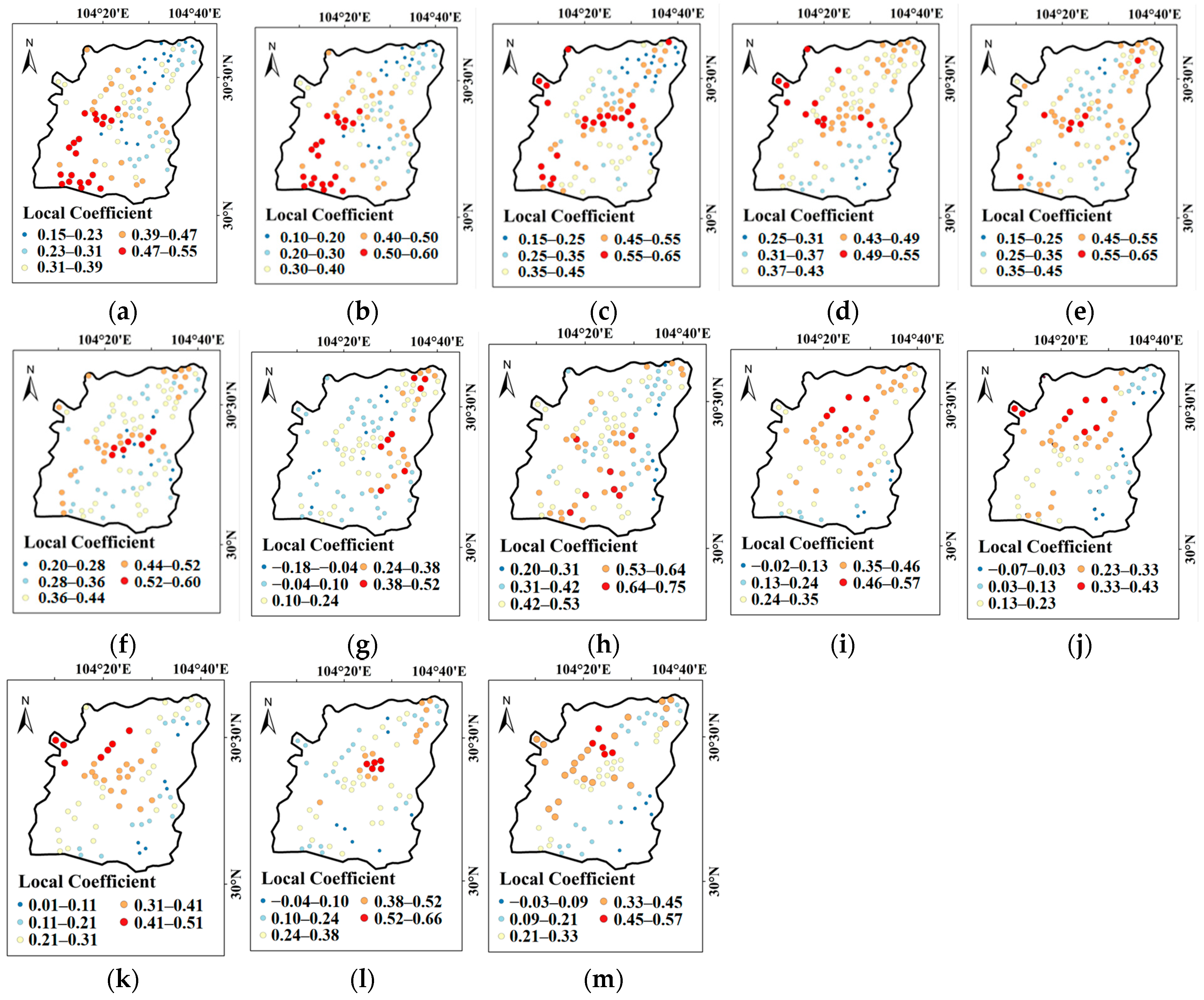
In this study, the MGWR model was employed to characterize the spatially non-stationary impacts of the investigated driving factors on soil HM accumulation across the study area. To ensure the statistical validity of the analysis, a variance inflation factor (VIF) test was initially conducted to screen for multicollinearity, where variables with a VIF > 10 are typically eliminated [112]. Since the VIF values for all 13 driving factors in this study were strictly less than 10, indicating the absence of significant multicollinearity, they were all retained for subsequent spatial modeling. The analysis was then implemented using the MGWR software, employing a Gaussian kernel function for spatial weighting and an AICc-minimized golden-section search algorithm for optimal bandwidth selection. Finally, the model was calibrated using the back-fitting algorithm proposed by Fotheringham et al. [76]. Spatially, As exhibits significant positive correlations with CC in the northern and southern regions and with AP in the central and southern regions (Figure 8a,b). This distribution pattern is likely driven by the strong As adsorption capacity of fine clay particles within the local purple soils, coupled with the sustained application of trace As-bearing agricultural fertilizers. Similarly, Cd is significantly and positively correlated with AP and PM_2.5 in the central-southern and central-western parts, respectively (Figure 8c,d). These associations are likely governed by Cd-containing agrochemical inputs alongside the monsoonal long-range transport of Cd-enriched fine particulate matter. Regarding Cu, significant positive correlations with SOM, CC, and pH are observed in the central, central-eastern, and northern areas of the study region, respectively (Figure 8e–g). This spatial heterogeneity is primarily dictated by the robust retention capacity of the soil organic carbon pool. Finally, Hg demonstrates a significant positive correlation with SOM across the central and southern regions (Figure 8h). This localized accumulation is largely attributable to the sequestration of Hg by SOM. For Cr, significant positive correlations with CC, elevation, and pH are notably clustered in the northern and northwestern sectors of the study area (Figure 8i–k). This distinct spatial configuration suggests that Cr distribution is primarily governed by natural pedogenic processes, where topographical variations and alkaline conditions facilitate the weathering of parent materials, with clay minerals acting as the main retention sites. In contrast, the spatial distribution of Pb is significantly influenced by SOM and PM_2.5, with the most pronounced positive correlations concentrated in the central region (Figure 8l,m). This localized pattern strongly implies an anthropogenically driven mechanism, wherein atmospheric Pb emissions are deposited as fine particulate matter and subsequently sequestered by the strong binding capacity of the local soil organic carbon pool.

3.5. Limitations and Prospects of the Proposed Method

To further validate the predictive superiority of the proposed HASM–ANN, its performance was benchmarked against the standard HASM and three conventional spatial interpolation techniques (OK, UK, and IDW). To achieve the optimal mapping accuracy for the spatial distribution of soil heavy metals, the parameters of the four interpolation models were rigorously calibrated through iterative experimentation. In the OK procedure, prior to variogram modeling, a log-transformation was applied to the highly skewed concentration data of Pb, Hg, and As to satisfy the normality assumption, whereas the remaining elements were processed using their untransformed data. A spherical semi-variogram model was subsequently selected for OK. To ensure an accurate representation of spatial autocorrelation, the lag size was configured to approximately 1/2 to 2/3 of the average minimum sampling distance, with the number of lags specified between 10 and 12. For the UK to account for spatial non-stationarity, a first-order polynomial was selected as the trend model, and the residuals were fitted using an exponential semi-variogram. The remaining parameters were kept consistent with those of the OK model. Lastly, for IDW, the distance power exponent was set to two. To account for the relatively sparse sample size and prevent excessive localized smoothing, the search neighborhood was defined using a “fixed number of points” strategy, specifically utilizing the 12 to 15 nearest neighbors for each prediction location. For the HASM model, the interpolation surfaces previously generated by the OK, UK, and IDW models were utilized as the iteration initial values. To achieve the optimal mapping accuracy for the spatial distribution of soil HMs, iterative parameter tuning was conducted. Specifically, the weight parameter, which controls the influence of the sampling points relative to the driving field, was set to 0.5. The relaxation coefficient, governing the flexibility of grid boundary constraints based on neighboring extreme values, was specified as 0.6. Furthermore, the local search neighborhood for boundary calculations was fixed at five adjacent points. Lastly, additional smoothing measures were deactivated to preserve the natural spatial heterogeneity of the raw concentration data. A comprehensive comparison of the accuracy metrics for these methods is detailed in

Table 6. Comparative accuracy mapping of ordinary kriging (OK), universal kriging (UK), inverse distance weighting (IDW), and HASM for soil heavy metals.

Element	OK		UK		IDW		HASM
	R2	RMSE	R2	RMSE	R2	RMSE	R2	RMSE
As 1	0.58	2.47	0.57	2.47	0.61	2.41	0.69	2.34
Cd 2	0.65	0.14	0.69	0.12	0.68	0.12	0.71	0.11
Cu 3	0.65	8.70	0.66	8.93	0.64	9.03	0.69	7.30
Hg 4	0.53	0.10	0.54	0.09	0.51	0.10	0.57	0.08
Cr 5	0.67	13.85	0.68	13.62	0.69	13.49	0.75	12.10
Pb 6	0.63	6.82	0.64	6.75	0.65	6.65	0.71	5.85

¹ Arsenic; ² Cadmium; ³ Copper; ⁴ Mercury; ⁵ Chromium; ⁶ Lead.

.

Previous studies have extensively applied traditional spatial interpolation methods to map the distribution of soil heavy metals, achieving varying degrees of accuracy. For instance, Ju et al. utilized IDW to map soil HM concentrations near a smelter in Henan Province, central China, reporting R² values of 0.74, 0.79, and 0.76 for Pb, Cd, and Cr, respectively [113]. Similarly, research by Xia et al. evaluated the OK model using soil samples from the Fuyang District in eastern China, yielding R² values of 0.55 for Pb, 0.60 for Cd, 0.66 for Cr, and 0.44 for As [114]. The constrained accuracy of these conventional models mainly stems from their inherent methodological limitations. Traditional methods, including OK, IDW, and UK, rely predominantly on the geographical coordinates of the sampling points. This direct, distance-based interpolation tends to overlook crucial environmental auxiliary variables. Given that the spatial heterogeneity of soil heavy metals is deeply driven by complex natural mechanisms relying solely on spatial distance without integrating these underlying natural driving factors inevitably restricts the models’ predictive capacity and their ability to accurately represent local spatial details [115].

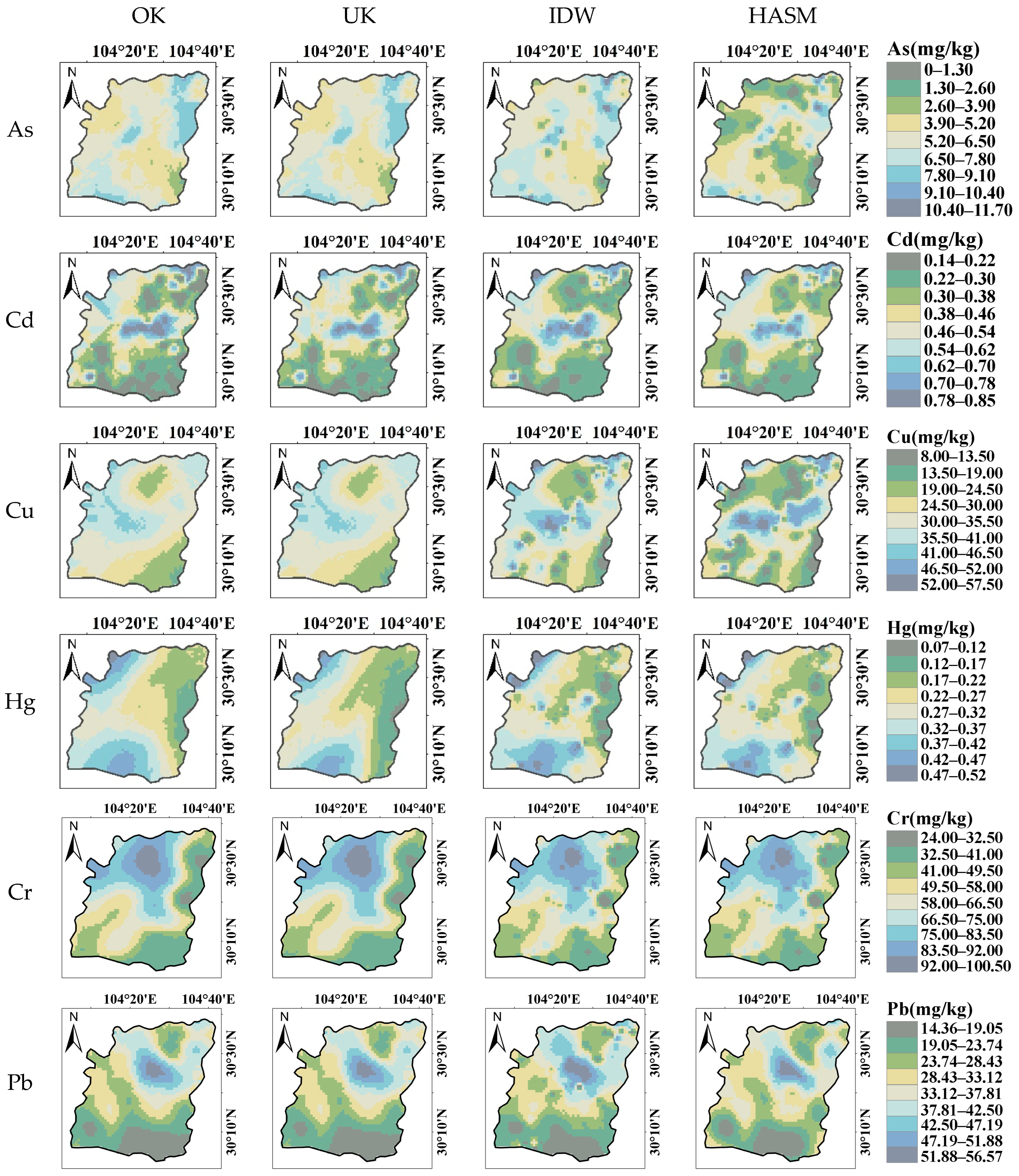
In contrast to the three conventional techniques, HASM significantly mitigates algorithmic biases, yielding superior predictive accuracy and minimizing deviation for soil HM mapping. This enhanced performance is evidenced by R² values spanning 0.57 to 0.71 and RMSE scores constrained between 0.081 and 7.298 mg/kg. The robustness of HASM stems from its least-squares optimization framework, which inherently resolves fundamental interpolation errors, multiscale complexities, and nonlinear spatial relationships [116]—a capability previously corroborated in the continuous spatial modeling of soil HMs [117]. However, previous studies have indicated that the HASM approach also has its inherent limitations. For example, Liu et al. [118] observed that the HASM’s effectiveness in characterizing soil properties can be compromised by inadequate interpolation precision and restricted adaptability. Jiang et al. [52] argued that the HASM’s reliance on oversimplified assumptions—specifically focusing on vertical and horizontal elevation gradients—often fails to capture the intricate directional fluctuations of natural surfaces, despite its proficiency in resolving amplitude-related undulations. Furthermore, when applied to high spatial resolution precipitation downscaling, the standard HASM frequently struggles to incorporate scale effects and auxiliary covariates, thereby limiting its capacity to refine downscaled remote sensing products [54]. As depicted in Figure 9, the four methods reveal distinct spatial patterns of soil HM contamination. Despite sharing similar global distributions, HASM-ANN and the HASM differ markedly in their local predictive capabilities. Specifically, the latter exhibits diminished accuracy in regions with low sampling density. However, the proposed HASM-ANN (Figure 5) effectively mitigates these limitations, demonstrating superior performance in handling unevenly distributed datasets and delivering higher spatial resolution in complex environments.

While the effectiveness of the HASM-ANN approach in mapping soil HMs, several directions for future improvement remain. First, addressing the limitations of sparse sampling and coarse environmental data is essential, particularly in regions with complex terrains. Integrating multi-source datasets from advanced satellites, such as the Sentinel series, offers a promising way to improve the spatiotemporal resolution of predictive variables and capture finer soil variations. Second, the computational complexity and time costs associated with building sophisticated hybrid models should be addressed. Future research should focus on balancing mapping precision with operational efficiency by developing more streamlined or parallelized coupling algorithms. Furthermore, the integration of HASM with a broader range of machine learning engines could further improve the ability to handle non-linear relationships and residuals in soil-environment systems. Finally, exploring the uncertainty of multi-source data within the HASM framework will be a key step toward providing more reliable spatial information for soil management and environmental protection. Furthermore, the aqueous solubility of HMs in agricultural soils carries meaningful environmental implications. It has recently garnered widespread attention as it can uncover the intrinsic link between HM speciation and leaching mechanisms in agricultural soils [119], accurately predict the migration risk of HMs toward groundwater systems [120], and effectively characterize the bioavailability of water-soluble fractions accumulated in crops via root uptake [121]. Building upon the HM concentrations in agricultural soils investigated in this study, future research could benefit from exploring the relationship between the aqueous solubility of HMs and their migration capacity, as well as the extent of contamination in agriculture.

In the future, the soil HM management should combine source control, risk-based zoning, and site-specific mitigation. Agricultural input regulation and atmospheric emission control should be strengthened in key risk areas. Suitable remediation measures, long-term monitoring, crop safety assessment, responsibility mechanisms, and special funding should also be established.

4. Conclusions

This study developed a novel hybrid downscaling framework, HASM-ANN, to finely map the spatial distribution of agricultural soil HMs (As, Cd, Cu, Hg, Cr, and Pb) in the eastern Longquan Mountain region, Chengdu, and quantitatively elucidated their underlying drivers. The HASM-ANN model effectively overcame the smoothing limitations of conventional interpolations (OK, UK, IDW), outperforming other machine learning hybrids with a superior predictive accuracy (R²: 0.75–0.86) and consistently achieved a significantly lower RMSE across all targeted soil heavy metals compared to the HASM. The HASM-ANN framework significantly enhances the accuracy of soil HMs mapping, providing a robust and reliable technical paradigm for regional agricultural contamination mapping and targeted environmental management. Furthermore, the GD and MGWR model analysis demonstrated that these spatial patterns are profoundly governed by the synergistic coupling of anthropogenic inputs and intrinsic soil properties. Specifically, strong non-linear enhancement interactions—such as AP combined with CC for As, PM_2.5 coupled with AP for Cd or SOM for Hg, SOM integrated with CC and pH for Cu, CC interacting with elevation and pH for Cr, and SOM paired with PM_2.5 for Pb—confirmed that localized enrichment is exacerbated by the interplay of external emissions and internal soil retention capacities.

References

1. Peng, Y.; Yu, G.I. Assessment of heavy metal pollution on agricultural land in Chengdu city under different anthropogenic pressures based on APCS-MLR modelling. Ecol. Indic. 2024, 165, 112183. [Google Scholar] [CrossRef]
2. Liu, Z.; Lu, Y.; Peng, Y.; Zhao, L.; Wang, G.; Hu, Y. Estimation of soil heavy metal content using hyperspectral data. Remote Sens. 2019, 11, 1464. [Google Scholar] [CrossRef]
3. Zhao, F.-J.; Ma, Y.; Zhu, Y.-G.; Tang, Z.; McGrath, S.P. Soil contamination in China: Current status and mitigation strategies. Environ. Sci. Technol. 2015, 49, 750–759. [Google Scholar] [CrossRef]
4. Wan, Y.; Liu, J.; Zhuang, Z.; Wang, Q.; Li, H. Heavy metals in agricultural soils: Sources, influencing factors, and remediation strategies. Toxics 2024, 12, 63. [Google Scholar] [CrossRef]
5. Ma, Y.; Su, Q.; Yue, C.; Zou, H.; Zhu, J.; Zhao, H.; Song, R.; Liu, Z. The effect of oxidative stress-induced autophagy by cadmium exposure in kidney, liver, and bone damage, and neurotoxicity. Int. J. Mol. Sci. 2022, 23, 13491. [Google Scholar] [CrossRef]
6. Park, R.M.; Bena, J.F.; Stayner, L.T.; Smith, R.J.; Gibb, H.J.; Lees, P.S.J. Hexavalent chromium and lung cancer in the chromate industry: A quantitative risk assessment. Risk Anal. 2004, 24, 1099–1108. [Google Scholar] [CrossRef]
7. Itoh, H.; Iwasaki, M.; Sawada, N.; Takachi, R.; Kasuga, Y.; Yokoyama, S.; Onuma, H.; Nishimura, H.; Kusama, R.; Kazuhito, Y.; et al. Dietary cadmium intake and breast cancer risk in Japanese women: A case–control study. Int. J. Hyg. Environ. Health 2014, 217, 70–77. [Google Scholar] [CrossRef]
8. Kapaj, S.; Peterson, H.; Liber, K.; Bhattacharya, P. Human health effects from chronic arsenic poisoning—A review. J. Environ. Sci. Health Part A 2006, 41, 2399–2428. [Google Scholar] [CrossRef]
9. Lin, H.-J.; Sung, T.-I.; Chen, C.-Y.; Guo, H.-R. Arsenic levels in drinking water and mortality of liver cancer in Taiwan. J. Hazard. Mater. 2013, 262, 1132–1138. [Google Scholar] [CrossRef] [PubMed]
10. Shi, P.; Xiao, J.; Wang, Y.; Chen, L. Assessment of ecological and human health risks of heavy metal contamination in agriculture soils disturbed by pipeline construction. Int. J. Environ. Res. Public Health 2014, 11, 2504–2520. [Google Scholar] [CrossRef] [PubMed]
11. Rashid, A.; Schutte, B.J.; Ulery, A.L.; Deyholos, M.K.; Sanogo, S.; Lehnhoff, E.A.; Beck, L. Heavy metal contamination in agricultural soil: Environmental pollutants affecting crop health. Agronomy 2023, 13, 1521. [Google Scholar] [CrossRef]
12. Tariq, M.; Iqbal, B.; Khan, I.; Khan, A.R.; Jho, E.H.; Salam, A.; Zhou, H.; Zhao, X.; Li, G.; Du, D. Microplastic contamination in the agricultural soil—Mitigation strategies, heavy metals contamination, and impact on human health: A review. Plant Cell Rep. 2024, 43, 65. [Google Scholar] [CrossRef]
13. Li, X.; Liu, H.; Meng, W.; Liu, N.; Wu, P. Accumulation and source apportionment of heavy metal(loid)s in agricultural soils based on GIS, SOM and PMF: A case study in superposition areas of geochemical anomalies and zinc smelting, Southwest China. Process Saf. Environ. Prot. 2022, 159, 964–977. [Google Scholar] [CrossRef]
14. Zeng, S.; Ma, J.; Yang, Y.; Zhang, S.; Liu, G.-J.; Chen, F. Spatial assessment of farmland soil pollution and its potential human health risks in China. Sci. Total Environ. 2019, 687, 642–653. [Google Scholar] [CrossRef] [PubMed]
15. El Behairy, R.A.; El Baroudy, A.A.; Ibrahim, M.M.; Mohamed, E.S.; Rebouh, N.Y.; Shokr, M.S. Combination of GIS and multivariate analysis to assess the soil heavy metal contamination in some arid zones. Agronomy 2022, 12, 2871. [Google Scholar] [CrossRef]
16. Shi, T.; Guo, L.; Chen, Y.; Wang, W.; Shi, Z.; Li, Q.; Wu, G. Proximal and remote sensing techniques for mapping of soil contamination with heavy metals. Appl. Spectrosc. Rev. 2018, 53, 783–805. [Google Scholar] [CrossRef]
17. Ha, H.; Olson, J.R.; Bian, L.; Rogerson, P.A. Analysis of heavy metal sources in soil using kriging interpolation on principal components. Environ. Sci. Technol. 2014, 48, 4999–5007. [Google Scholar] [CrossRef] [PubMed]
18. Lovynska, V.; Bayat, B.; Bol, R.; Moradi, S.; Rahmati, M.; Raj, R.; Sytnyk, S.; Wiche, O.; Wu, B.; Montzka, C. Monitoring heavy metals and metalloids in soils and vegetation by remote sensing: A review. Remote Sens. 2024, 16, 3221. [Google Scholar] [CrossRef]
19. Liu, K.; Zhao, D.; Fang, J.-Y.; Zhang, X.; Zhang, Q.-Y.; Li, X.-K. Estimation of heavy-metal contamination in soil using remote sensing spectroscopy and a statistical approach. J. Indian Soc. Remote Sens. 2017, 45, 805–813. [Google Scholar] [CrossRef]
20. Yang, Y.; Jia, M. 3D spatial interpolation of soil heavy metals by combining kriging with depth function trend model. J. Hazard. Mater. 2023, 461, 132571. [Google Scholar] [CrossRef]
21. Qiao, P.; Lei, M.; Yang, S.; Yang, J.; Guo, G.; Zhou, X. Comparing ordinary kriging and inverse distance weighting for soil as pollution in Beijing. Environ. Sci. Pollut. Res. Int. 2018, 25, 15597–15608. [Google Scholar] [CrossRef]
22. Han, H.; Suh, J. Spatial prediction of soil contaminants using a hybrid random forest–ordinary kriging model. Appl. Sci. 2024, 14, 1666. [Google Scholar] [CrossRef]
23. Khan, M.; Almazah, M.M.A.; EIlahi, A.; Niaz, R.; Al-Rezami, A.Y.; Zaman, B. Spatial interpolation of water quality index based on Ordinary kriging and Universal kriging. Geomat. Nat. Hazards Risk 2023, 14, 2190853. [Google Scholar] [CrossRef]
24. Mohamoud, A.M.; Halder, B.; Shakir, H.S.; Yaseen, Z.M. Soil heavy metal contamination analysis: A representative case study in New Zealand. J. Environ. Chem. Eng. 2025, 13, 116808. [Google Scholar] [CrossRef]
25. Zheng, Q.; Gao, X.; Qi, Y.; Li, J. Spatial distribution of heavy metal contamination in mollisol dairy farm. Environ. Pollut. 2020, 263, 114621. [Google Scholar] [CrossRef]
26. Man, J.; Zeng, L.; Luo, J.; Gao, W.; Yao, Y. Application of the deep learning algorithm to identify the spatial distribution of heavy metals at contaminated sites. ACS Es&T Engg. 2022, 2, 158–168. [Google Scholar] [CrossRef]
27. Goovaerts, P. Kriging and semivariogram deconvolution in the presence of irregular geographical units. Math. Geosci. 2008, 40, 101–128. [Google Scholar] [CrossRef]
28. Magnussen, S.; Næsset, E.; Wulder, M.A. Efficient multiresolution spatial predictions for large data arrays. Remote Sens. Environ. 2007, 109, 451–463. [Google Scholar] [CrossRef]
29. Yue, T.X.; Wang, S.H. Adjustment computation of HASM: A high-accuracy and high-speed method. Int. J. Geogr. Inf. Sci. 2010, 24, 1725–1743. [Google Scholar] [CrossRef]
30. Yue, T.X. Surface Modeling: High Accuracy and High Speed Methods; CRC Press: New York, NY, USA, 2011. [Google Scholar]
31. Yue, T.X.; Zhang, L.L.; Zhao, N.; Zhao, M.W.; Chen, C.F.; Du, Z.P.; Song, D.J.; Fan, Z.M.; Shi, W.J.; Wang, S.H.; et al. A review of recent developments in HASM. Environ. Earth Sci. 2015, 74, 6541–6549. [Google Scholar] [CrossRef]
32. Chen, C.F.; Yue, T.X.; Dai, H.L.; Tian, M.Y. The smoothness of HASM. Int. J. Geogr. Inf. Sci. 2013, 27, 1651–1667. [Google Scholar] [CrossRef]
33. Shi, W.; Liu, J.; Du, Z.; Song, Y.; Chen, C.; Yue, T. Surface modelling of soil pH. Geoderma 2009, 150, 113–119. [Google Scholar] [CrossRef]
34. Zhou, W.; Wang, T.; Peng, Y.; Yu, W.; Sun, X.; Tian, Y.; Li, S.; Du, Z.; Yue, T. Data fusion enhances the accuracy of soil organic carbon estimation by using high accuracy surface modeling. Soil Tillage Res. 2025, 261, 106945. [Google Scholar] [CrossRef]
35. Senanayake, I.P.; Pathira Arachchilage, K.R.L.; Yeo, I.-Y.; Khaki, M.; Han, S.-C.; Dahlhaus, P.G. Spatial downscaling of satellite-based soil moisture products using machine learning techniques: A review. Remote Sens. 2024, 16, 2067. [Google Scholar] [CrossRef]
36. Srivastava, P.K.; Han, D.; Rico-Ramirez, M.A.; Islam, T. Machine learning techniques for downscaling SMOS satellite soil moisture using MODIS land surface temperature for hydrological application. Water Resour. Manag. 2013, 27, 3127–3144. [Google Scholar] [CrossRef]
37. Tripathi, S.; Srinivas, V.V.; Nanjundiah, R.S. Downscaling of precipitation for climate change scenarios: A support vector machine approach. J. Hydrol. 2006, 330, 621–640. [Google Scholar] [CrossRef]
38. Luo, Q.; Liang, Y.; Guo, Y.; Liang, X.; Ren, C.; Yue, W.; Zhu, B.; Jiang, X. Enhancing spatial resolution of GNSS-R soil moisture retrieval through XGBoost algorithm-based downscaling approach: A case study in the Southern United States. Remote Sens. 2023, 15, 4576. [Google Scholar] [CrossRef]
39. Chen, Q.; Miao, F.; Wang, H.; Xu, Z.-X.; Tang, Z.; Yang, L.; Qi, S. Downscaling of satellite remote sensing soil moisture products over the Tibetan Plateau based on the random forest algorithm: Preliminary results. Earth Space Sci. 2020, 7, e2020EA001265. [Google Scholar] [CrossRef]
40. GB 15618-2018; Soil Environmental Quality Risk Control Standard for Soil Contamination of Agricultural Land. Standardization Administration: Beijing, China, 2018.
41. Huang, Y.; Wang, L.; Wang, W.; Li, T.; He, Z.; Yang, X. Current status of agricultural soil pollution by heavy metals in China: A meta-analysis. Sci. Total Environ. 2019, 651, 3034–3042. [Google Scholar] [CrossRef]
42. Moraru, S.-S.; Ene, A.; Stihi, C.; Dulama, I.-D. ICP-MS study of metal (Cd, Co, Cr, Cu, Fe, Mn, Ni, Pb, Al, Sr, Li, Zn, Ag) contamination of soils nearby steel industry and their transfer to crops. Rom. J. Phys. 2025, 70, 803. [Google Scholar] [CrossRef]
43. Peng, S.; Ding, Y.; Liu, W.; Li, Z. 1 km monthly temperature and precipitation dataset for China from 1901 to 2017. Earth Syst. Sci. Data. 2019, 11, 1931–1946. [Google Scholar] [CrossRef]
44. Zhao, K.; Yan, D.; Qin, T.; Li, C.; Peng, D.; Song, Y. A 1 km daily high-accuracy meteorological dataset of air temperature, atmospheric pressure, relative humidity, and sunshine duration across China (1961–2021). Earth Syst. Sci. Data. 2025, 17, 7251–7270. [Google Scholar] [CrossRef]
45. Wei, J.; Li, Z.; Lyapustin, A.; Sun, L.; Peng, Y.; Xue, W.; Su, T.; Cribb, M. Reconstructing 1-km-resolution high-quality PM2.5 data records from 2000 to 2018 in China: Spatiotemporal variations and policy implications. Remote Sens. Environ. 2021, 252, 112136. [Google Scholar] [CrossRef]
46. Jamaludin, N.N.J.; Abdullah, A.F.; Muhadi, N.N.A.; Wayayok, A. Assessment and enhancement of Landsat 8 land surface temperature retrieval using mono window algorithm and machine learning approaches. J. Atmos. Sol.-Terr. Phys. 2025, 276, 106618. [Google Scholar] [CrossRef]
47. Kumar, B.P.; Babu, K.R.; Anusha, B.N.; Rajasekhar, M. Geo-environmental monitoring and assessment of land degradation and desertification in the semi-arid regions using Landsat 8 OLI/TIRS, LST, and NDVI approach. Environ. Chall. 2022, 8, 100578. [Google Scholar] [CrossRef]
48. Li, P.; Xiao, C.; Feng, Z. Mapping rice planted area using a new normalized EVI and SAVI (NVI) derived from Landsat-8 OLI. IEEE Geosci. Remote Sens. Lett. 2018, 15, 1822–1826. [Google Scholar] [CrossRef]
49. Wu, Z.; Yao, F.; Zhang, J.; Liu, H. Estimating forest aboveground biomass using a combination of geographical random forest and empirical Bayesian kriging models. Remote Sens. 2024, 16, 1859. [Google Scholar] [CrossRef]
50. Mancino, G.; Ferrara, A.; Padula, A.; Nolè, A. Cross-comparison between Landsat 8 (OLI) and Landsat 7 (ETM+) derived vegetation indices in a Mediterranean environment. Remote Sens. 2020, 12, 291. [Google Scholar] [CrossRef]
51. Marsett, R.C.; Qi, J.; Heilman, P.; Biedenbender, S.H.; Watson, M.C.; Amer, S.; Weltz, M.; Goodrich, D.; Marsett, R. Remote sensing for grassland management in the arid Southwest. Rangel. Ecol. Manag. 2006, 59, 530–540. [Google Scholar] [CrossRef]
52. Jiang, L.; Zhao, M.; Yue, T.; Zhao, N.; Wang, C.; Sun, J. A modified HASM algorithm and its application in DEM construction. Earth Sci. Inform. 2018, 11, 423–431. [Google Scholar] [CrossRef]
53. Zhao, N.; Yue, T.X. A modification of HASM for interpolating precipitation in China. Theor. Appl. Climatol. 2014, 116, 273–285. [Google Scholar] [CrossRef]
54. Zhao, N.; Jiao, Y. A new HASM-based downscaling method for high-resolution precipitation estimates. Remote Sens. 2021, 13, 2693. [Google Scholar] [CrossRef]
55. Jordan, M.I.; Mitchell, T.M. Machine learning: Trends, perspectives, and prospects. Science 2015, 349, 255–260. [Google Scholar] [CrossRef] [PubMed]
56. Shi, S.; Hou, M.; Gu, Z.; Jiang, C.; Zhang, W.; Hou, M.; Li, C.; Xi, Z. Estimation of heavy metal content in soil based on machine learning models. Land 2022, 11, 1037. [Google Scholar] [CrossRef]
57. Zhao, P.; Li, K.; Zhou, N.; Chen, Q.; Zhou, M.; Qi, C. Enhanced prediction of occurrence forms of heavy metals in tailings: A systematic comparison of machine learning methods and model integration. Int. J. Miner. Metall. Mater. 2025, 32, 2406–2417. [Google Scholar] [CrossRef]
58. Wang, H.; Yilihamu, Q.; Yuan, M.; Bai, H.; Xu, H.; Wu, J. Prediction models of soil heavy metal(loid)s concentration for agricultural land in Dongli: A comparison of regression and random forest. Ecol. Indic. 2020, 119, 106801. [Google Scholar] [CrossRef]
59. Ye, M.; Zhu, L.; Li, X.; Ke, Y.; Huang, Y.; Chen, B.; Yu, H.; Li, H.; Feng, H. Estimation of the soil arsenic concentration using a geographically weighted XGBoost model based on hyperspectral data. Sci. Total Environ. 2023, 858, 159798. [Google Scholar] [CrossRef]
60. Mahmood, T.; Löw, J.; Pöhlitz, J.; Wenzel, J.L.; Conrad, C. Estimation of 100 m root zone soil moisture by downscaling 1 km soil water index with machine learning and multiple geodata. Environ. Monit. Assess. 2024, 196, 823. [Google Scholar] [CrossRef]
61. Zhou, J.; Liu, S.; Li, M.; Zhan, W.; Xu, Z.; Xu, T. Quantification of the scale effect in downscaling remotely sensed land surface temperature. Remote Sens. 2016, 8, 975. [Google Scholar] [CrossRef]
62. Ershadi, A.; McCabe, M.F.; Evans, J.P.; Walker, J.P. Effects of spatial aggregation on the multi-scale estimation of evapotranspiration. Remote Sens. Environ. 2013, 131, 51–62. [Google Scholar] [CrossRef]
63. Alemohammad, S.H.; Kolassa, J.; Prigent, C.; Aires, F.; Gentine, P. Global downscaling of remotely sensed soil moisture using neural networks. Hydrol. Earth. Syst. Sci. 2018, 22, 5341–5356. [Google Scholar] [CrossRef]
64. Zhao, W.; Ma, J.; Liu, Q.; Dou, L.; Qu, Y.; Shi, H.; Sun, Y.; Chen, H.; Tian, Y.; Wu, F. Accurate prediction of soil heavy metal pollution using an improved machine learning method: A case study in the Pearl River Delta, China. Environ. Sci. Technol. 2023, 57, 17751–17761. [Google Scholar] [CrossRef]
65. Jin, Y.; Ge, Y.; Liu, Y.; Chen, Y.; Zhang, H.; Heuvelink, G.B.M. A machine learning-based geostatistical downscaling method for coarse-resolution soil moisture products. IEEE J. Sel. Top. Appl. Earth Obs. Remote Sens. 2021, 14, 1025–1037. [Google Scholar] [CrossRef]
66. Chang, C.-C.; Lin, C.-J. LIBSVM: A library for support vector machines. ACM Trans. Intell. Syst. Technol. 2011, 2, 1–27. [Google Scholar] [CrossRef]
67. Zhao, W.; Sánchez, N.; Lu, H.; Li, A. A spatial downscaling approach for the SMAP passive surface soil moisture product using random forest regression. J. Hydrol. 2018, 563, 1009–1024. [Google Scholar] [CrossRef]
68. Taghizadeh-Mehrjardi, R.; Fathizad, H.; Ali Hakimzadeh Ardakani, M.; Sodaiezadeh, H.; Kerry, R.; Heung, B.; Scholten, T. Spatio-temporal analysis of heavy metals in arid soils at the catchment scale using digital soil assessment and a random forest model. Remote Sens. 2021, 13, 1698. [Google Scholar] [CrossRef]
69. Li, X.; Gu, H.; Tang, R.; Zou, B.; Liu, X.; Ou, H.; Chen, X.; Song, Y.; Luo, W.; Wen, B. A fusion XGBoost approach for large-scale monitoring of soil HM in farmland using hyperspectral imagery. Agronomy 2025, 15, 676. [Google Scholar] [CrossRef]
70. Zhu, H.; Liu, H.; Zhou, Q.; Cui, A. A XGBoost-based downscaling-calibration scheme for extreme precipitation events. IEEE Trans. Geosci. Remote Sens. 2023, 61, 4103512. [Google Scholar] [CrossRef]
71. Chicco, D.; Warrens, M.J.; Jurman, G. The coefficient of determination R-squared is more informative than SMAPE, MAE, MAPE, MSE and RMSE in regression analysis evaluation. PeerJ Comput. Sci. 2021, 7, e623. [Google Scholar] [CrossRef]
72. Lloyd, C.D. Assessing the effect of integrating elevation data into the estimation of monthly precipitation in Great Britain. J. Hydrol. 2005, 308, 128–150. [Google Scholar] [CrossRef]
73. Liu, Y.; Zhang, W.; Zhang, Z.; Xu, Q.; Li, W. Risk factor detection and landslide susceptibility mapping using Geo-Detector and Random Forest models: The 2018 Hokkaido Eastern Iburi earthquake. Remote Sens. 2021, 13, 1157. [Google Scholar] [CrossRef]
74. Wang, J.F.; Li, X.H.; Christakos, G.; Liao, Y.-L.; Zhang, T.; Gu, X.; Zheng, X. Geographical detectors-based health risk assessment and its application in the neural tube defects study of the Heshun Region, China. Int. J. Geogr. Inf. Sci. 2010, 24, 107–127. [Google Scholar] [CrossRef]
75. Zhang, L.; Su, Y.; Li, Y.; Lin, P. Estimating urban land subsidence with satellite data using a spatially multiscale geographically weighted regression approach. Measurement 2024, 228, 114387. [Google Scholar] [CrossRef]
76. Fotheringham, A.S.; Yang, W.; Kang, W. Multiscale geographically weighted regression (MGWR). Ann. Am. Assoc. Geogr. 2017, 107, 1247–1265. [Google Scholar] [CrossRef]
77. Zhu, H.; Zhou, Q.; Cui, A. Comparison and evaluation of machine-learning-based spatial downscaling approaches on satellite-derived precipitation data. ISPRS Ann. Photogramm. Remote Sens. Spat. Inf. Sci. 2023, 10, 919–924. [Google Scholar] [CrossRef]
78. Khosravi, V.; Doulati Ardejani, F.; Yousefi, S.; Aryafar, A. Monitoring soil lead and zinc contents via combination of spectroscopy with extreme learning machine and other data mining methods. Geoderma 2018, 318, 29–41. [Google Scholar] [CrossRef]
79. Hateffard, F.; Steinbuch, L.; Heuvelink, G.B.M. Evaluating the extrapolation potential of random forest digital soil mapping. Geoderma 2024, 441, 116740. [Google Scholar] [CrossRef]
80. Grekousis, G. Geographical-XGBoost: A new ensemble model for spatially local regression based on gradient-boosted trees. J. Geogr. Syst. 2025, 27, 169–195. [Google Scholar] [CrossRef]
81. Anagu, I.; Ingwersen, J.; Utermann, J.; Streck, T. Estimation of heavy metal sorption in German soils using artificial neural networks. Geoderma 2009, 152, 104–112. [Google Scholar] [CrossRef]
82. Naderi, A.; Delavar, M.A.; Kaboudin, B.; Askari, M.S. Assessment of spatial distribution of soil heavy metals using ANN-GA, MSLR and satellite imagery. Environ. Monit. Assess. 2017, 189, 214. [Google Scholar] [CrossRef]
83. Nourani, V.; Razzaghzadeh, Z.; Hosseini Baghanam, A.; Molajou, A. ANN-based statistical downscaling of climatic parameters using decision tree predictor screening method. Theor. Appl. Climatol. 2019, 137, 1729–1746. [Google Scholar] [CrossRef]
84. Lv, A.; Zhang, Z.; Zhu, H. A neural-network based spatial resolution downscaling method for soil moisture: Case study of Qinghai Province. Remote Sens. 2021, 13, 1583. [Google Scholar] [CrossRef]
85. Jiang, Z.; Yang, M.; Yang, L.; Su, W.; Liu, Z. Spatial–temporal evolution characteristics and driving mechanism analysis of the “three-zone space” in China’s Ili River Basin. Land 2024, 13, 1530. [Google Scholar] [CrossRef]
86. Mahimairaja, S.; Bolan, N.S.; Adriano, D.C.; Robinson, B. Arsenic contamination and its risk management in complex environmental settings. Adv. Agron. 2005, 86, 1–82. [Google Scholar] [CrossRef]
87. Wang, Y.; Zhang, L.; Wang, J.; Lv, J. Identifying quantitative sources and spatial distributions of potentially toxic elements in soils by using three receptor models and sequential indicator simulation. Chemosphere 2020, 242, 125266. [Google Scholar] [CrossRef]
88. Khatun, J.; Intekhab, A.; Dhak, D. Effect of uncontrolled fertilization and heavy metal toxicity associated with arsenic (As), lead (Pb) and cadmium (Cd), and possible remediation. Toxicology 2022, 477, 153274. [Google Scholar] [CrossRef]
89. Wang, K.; Yao, Y.; Mao, K. Seasonal variations of PM2.5 pollution in the Chengdu–Chongqing Urban Agglomeration, China. Sustainability 2024, 16, 9242. [Google Scholar] [CrossRef]
90. Luo, L.; Ma, Y.; Zhang, S.; Wei, D.; Zhu, Y.-G. An inventory of trace element inputs to agricultural soils in China. J. Environ. Manag. 2009, 90, 2524–2530. [Google Scholar] [CrossRef] [PubMed]
91. Jiang, H.-H.; Cai, L.-M.; Wen, H.-H.; Hu, G.-C.; Chen, L.-G.; Luo, J. An integrated approach to quantifying ecological and human health risks from different sources of soil heavy metals. Sci. Total Environ. 2020, 701, 134466. [Google Scholar] [CrossRef] [PubMed]
92. Bhuiyan, M.A.H.; Parvez, L.; Islam, M.A.; Dampare, S.B.; Suzuki, S. Heavy metal pollution of coal mine-affected agricultural soils in the northern part of Bangladesh. J. Hazard. Mater. 2010, 173, 384–392. [Google Scholar] [CrossRef] [PubMed]
93. Zhou, J.; Wang, Z.; Zhang, X.; Driscoll, C.T.; Lin, C.-J. Soil–atmosphere exchange flux of total gaseous mercury (TGM) at subtropical and temperate forest catchments. Atmos. Chem. Phys. 2020, 20, 16117–16133. [Google Scholar] [CrossRef]
94. Wang, X.; Sun, Y.; Guo, H.; Wang, H. Analysis of soil heavy metal Hg pollution source based on GeoDetector. Pol. J. Environ. Stud. 2022, 31, 501–510. [Google Scholar] [CrossRef]
95. Hu, H.; Zhou, W.; Liu, X.; Guo, G.; He, Y.; Zhu, L.; Chen, D.; Miao, R. Machine learning combined with geodetector to predict the spatial distribution of soil heavy metals in mining areas. Sci. Total Environ. 2025, 959, 178281. [Google Scholar] [CrossRef]
96. Jung, C.-C.; Chiang, T.-Y.; Chung, Y.-J.; Chou, C.C.-K.; Huang, Y.-T.; Chung, C.J. Lead (Pb) in PM2.5 exposure hotspots and pollution sources affecting adults and children in multiple urban environments. Build. Environ. 2025, 284, 113485. [Google Scholar] [CrossRef]
97. Cui, S.; Liu, L.; Zhang, F.; Fu, Q.; Ma, C.; Ding, Y. Compositional evolution of dissolved organic matter mobilized by straw incorporation and its climate-driven interactions with lead in cold-region black soil: Decoding mechanisms through PARAFAC and complexation modeling. Carbon Res. 2025, 4, 56. [Google Scholar] [CrossRef]
98. Marković, J.; Jović, M.; Smičiklas, I.; Pezo, L.; Šljivić-Ivanović, M.; Onjia, A. Chemical speciation of metals in unpolluted soils of different types: Correlation with soil characteristics and an ANN modelling approach. J. Geochem. Explor. 2016, 165, 71–80. [Google Scholar] [CrossRef]
99. Marković, J.; Jović, M.; Smičiklas, I.; Šljivić-Ivanović, M.; Onjia, A.; Trivunac, K.; Popović, A. Cadmium retention and distribution in contaminated soil: Effects and interactions of soil properties, contamination level, aging time and in situ immobilization agents. Ecotoxicol. Environ. Saf. 2019, 174, 305–314. [Google Scholar] [CrossRef]
100. Goldberg, S. Competitive adsorption of arsenate and arsenite on oxides and clay minerals. Soil Sci. Soc. Am. J. 2002, 66, 413–421. [Google Scholar] [CrossRef]
101. Park, J.; Lee, D.; Kim, H.; Woo, N.C. Effects of water-table changes following rainfall events on arsenic fate and transport in groundwater–surface water mixing zones. Sci. Total Environ. 2024, 933, 173200. [Google Scholar] [CrossRef]
102. Li, D.; Zheng, J.; Yang, M.; Meng, Y.; Yu, X.; Zhou, H.; Tong, L.; Wang, K.; Li, Y.; Wang, X.; et al. Atmospheric wet deposition of trace metal elements: Monitoring and modelling. Sci. Total Environ. 2023, 893, 164880. [Google Scholar] [CrossRef]
103. Sun, X.-L.; Wang, Y.; Xiong, H.-Q.; Wu, F.; Lv, T.-X.; Fang, Y.C.; Xiang, H. The role of surface functional groups of iron oxide, organic matter, and clay mineral complexes in sediments on the adsorption of copper ions. Sustainability 2023, 15, 6711. [Google Scholar] [CrossRef]
104. Wu, F.; Yang, L.; Wang, X.; Yuan, W.; Lin, C.-J.; Feng, X. Mercury accumulation and sequestration in a deglaciated forest chronosequence: Insights from particulate and mineral-associated forms of organic matter. Environ. Sci. Technol. 2023, 57, 16512–16521. [Google Scholar] [CrossRef]
105. Zhang, Z.-Y.; Li, G.; Yang, L.; Wang, X.-J.; Sun, G.-X. Mercury distribution in the surface soil of China is potentially driven by precipitation, vegetation cover and organic matter. Environ. Sci. Eur. 2020, 32, 89. [Google Scholar] [CrossRef]
106. Xue, W.; Wang, C.; Pan, S.; Zhang, C.; Huang, Y.; Liu, Z. Effects of elevation and geomorphology on cadmium, lead and chromium enrichment in paddy soil and rice: A case study in the Xiangtan basin of China. Sci. Total Environ. 2024, 912, 168613. [Google Scholar] [CrossRef] [PubMed]
107. Veselská, V.; Fajgar, R.; Číhalová, S.; Bolanz, R.M.; Göttlicher, J.; Steininger, R.; Siddique, J.A.; Komárek, M. Chromate adsorption on selected soil minerals: Surface complexation modeling coupled with spectroscopic investigation. J. Hazard. Mater. 2016, 318, 433–442. [Google Scholar] [CrossRef] [PubMed]
108. Gao, Q.; Zhu, S.; Zhou, K.; Zhai, J.; Chen, S.; Wang, Q.; Wang, S.; Han, J.; Lu, X.; Chen, H.; et al. High enrichment of heavy metals in fine particulate matter through dust aerosol generation. Atmos. Chem. Phys. 2023, 23, 13049–13060. [Google Scholar] [CrossRef]
109. Gustafsson, J.P.; Tiberg, C.; Edkymish, A.; Kleja, D.B. Modelling lead (II) sorption to ferrihydrite and soil organic matter. Environ. Chem. 2011, 8, 485–492. [Google Scholar] [CrossRef]
110. Cao, X.; Xu, Y.; Wang, F.; Zhang, Z.; Xu, X. Changes of soil organic carbon and aggregate stability along elevation gradient in Cunninghamia lanceolata plantations. Sci. Rep. 2024, 14, 31778. [Google Scholar] [CrossRef] [PubMed]
111. Yamada, N.; Katoh, M. Feature of lead complexed with dissolved organic matter on lead immobilization by hydroxyapatite in aqueous solutions and soils. Chemosphere 2020, 249, 126122. [Google Scholar] [CrossRef]
112. Lin, D.; Foster, D.P.; Ungar, L.H. VIF regression: A fast regression algorithm for large data. J. Am. Stat. Assoc. 2011, 106, 232–247. [Google Scholar] [CrossRef]
113. Ju, L.; Guo, S.; Ruan, X.; Wang, Y. Improving the mapping accuracy of soil heavy metals through an adaptive multi-fidelity interpolation method. Environ. Pollut. 2023, 330, 121827. [Google Scholar] [CrossRef]
114. Xia, F.; Hu, B.; Shao, S.; Xu, D.; Zhou, Y.; Zhou, Y.; Huang, M.; Li, Y.; Chen, S.; Shi, Z. Improvement of spatial modeling of Cr, Pb, Cd, As and Ni in soil based on portable X-ray fluorescence (PXRF) and geostatistics: A case study in East China. Int. J. Environ. Res. Public Health 2019, 16, 2694. [Google Scholar] [CrossRef]
115. Liu, C.; Chen, L.; Ni, G.; Yuan, X.; He, S.; Miao, S. Prediction of heavy metal spatial distribution in soils of typical industrial zones utilizing 3D convolutional neural networks. Sci. Rep. 2025, 15, 396. [Google Scholar] [CrossRef]
116. Mukherjee, S.; Joshi, P.K.; Garg, R.D. A comparison of different regression models for downscaling Landsat and MODIS land surface temperature images over heterogeneous landscape. Adv. Space Res. 2014, 54, 655–669. [Google Scholar] [CrossRef]
117. Yue, T.X.; Zhao, N.; Shi, W.J.; Fan, Z.M. Surface modelling of soil properties. In Eco-Environmental Informatics; Springer: Singapore, 2025. [Google Scholar] [CrossRef]
118. Liu, W.; Liu, Y.; Yang, M.; Xie, M. Soil property surface modeling based on ensemble learning for complex landforms. In Geo-Informatics in Sustainable Ecosystem and Society; Springer: Singapore, 2019; Volume 980, pp. 1–14. [Google Scholar] [CrossRef]
119. Wang, Z.; Tang, W.; Ding, X.; Dong, Q.; Guo, Y.; Liu, G.; Liu, Y.; Liang, Y.; Yin, Y.; Cai, Y.; et al. Different extractable pools of Cd and Pb in agricultural soil under amendments: Water-soluble concentration sensitively indicates metal availability. J. Environ. Sci. 2025, 150, 297–308. [Google Scholar] [CrossRef]
120. Sharafi, S.; Salehi, F. Comprehensive assessment of heavy metal (HMs) contamination and associated health risks in agricultural soils and groundwater proximal to industrial sites. Sci. Rep. 2025, 15, 7518. [Google Scholar] [CrossRef]
121. Feyisa, G.; Mekassa, B.; Merga, L.B. Human health risks of heavy metals contamination of a water-soil-vegetables farmland system in Toke Kutaye of West Shewa, Ethiopia. Toxicol. Rep. 2025, 14, 102061. [Google Scholar] [CrossRef]
Figure 1. Geographical location and sampling design of the eastern Longquan Mountain region study area: (a) topographic context across Chengdu, Meishan, and Ziyang City; (b) true-color satellite imagery of the region; and (c) spatial distribution of the calibration and validation sampling sites.
Applsci 16 05402 g001
Figure 2. Spatial distribution of potential driving factors for farmland soil heavy metals in the study area. (TEM: air temperature; PRE: precipitation; RH: relative humidity; LST: land surface temperature; NDVI: normalized difference vegetation index; CEC: cation exchange capacity; AP: available phosphorus; SC: sand content; CC: clay content; SOM: soil organic matter).
Applsci 16 05402 g002
Figure 3. Flowchart of the hybrid HASM–machine learning-based downscaling framework for farmland soil heavy metals.
Applsci 16 05402 g003
Figure 4. Comparison between the measured and estimated soil heavy metal concentrations.
Applsci 16 05402 g004
Figure 5. Spatial patterns of soil heavy metals by HASM–ANN at a 100 m spatial resolution in the study area.
Applsci 16 05402 g005
Figure 6. The q-values for each driving factor of the soil heavy metals in the study area.
Applsci 16 05402 g006
Figure 7. Interaction detection results among the driving factors for the soil heavy metals in the study area.
Applsci 16 05402 g007
Figure 8. Spatial distribution of local coefficients from the MGWR models. The maps depict the respective effects of the driving factors: (a) CC and (b) AP on As; (c) AP and (d) PM2.5 on Cd; (e) SOM, (f) CC, and (g) pH on Cu; (h) SOM on Hg; (i) CC, (j) pH, and (k) elevation on Cr; and (l) SOM and (m) PM2.5 on Pb.
Applsci 16 05402 g008
Figure 9. Soil heavy metal concentration interpolation results in the study area based on ordinary kriging (OK), universal kriging (UK), inverse distance weighting (IDW), and HASM.
Applsci 16 05402 g009