VDCrackGAN: A Generative Adversarial Network with Transformer for Pavement Crack Data Augmentation

Abstract

Addressing the challenge of limited samples arising from the difficulty and high cost of pavement crack, image collecting and labeling, along with the inadequate ability of traditional data augmentation methods to enhance sample feature space, we propose VDCrackGAN, a generative adversarial network combining VAE and DCGAN, specifically tailored for pavement crack data augmentation. Furthermore, spectral normalization is incorporated to enhance the stability of network training, and the self-attention mechanism Swin Transformer is integrated into the network to further improve the quality of crack generation. Experimental outcomes reveal that in comparison to the baseline DCGAN, VDCrackGAN achieves notable improvements of 13.6% and 26.4% in the Inception Score (IS) and Fréchet Inception Distance (FID) metrics, respectively.

1. Introduction

Cracks are the most prevalent type of pavement distress, representing an early stage of pavement degradation. If not repaired in time, they can rapidly evolve into more serious pavement distress, such as alligator cracks, looseness, or even potholes. Timely detection and repair of cracks are of great significance in preventing the deterioration of pavement damage and reducing pavement maintenance costs. Traditional crack detection relies heavily on visual inspection by engineering and technical personnel, which is subjective and inefficient [1]. In recent years, deep learning has achieved significant breakthroughs in the field of image recognition [2,3]. Many scholars have successfully applied convolutional neural networks (CNNs) to crack detection, significantly enhancing the efficiency and accuracy of crack detection [4,5].

However, deep learning methods are essentially data-driven approaches that require the support of a large amount of training sample data. In practice, it is difficult and expensive to collect and label pavement crack data, which results in a small-scale pavement crack dataset, thereby affecting the generalization ability and accuracy of the training model. In the case of insufficient training samples, it is necessary to investigate data augmentation methods specifically for crack detection.

Traditional data augmentation methods, such as rotation, brightness change, random cropping, etc., are essentially transformations based on certain rules applied to the original image. The distribution of the generated images tends to be relatively homogeneous, so although the number of samples is increased, the improvement in sample quality is limited. Another approach to data augmentation is to generate data directly based on generative deep learning models, such as variational autoencoders (VAEs) [6] and generative adversarial networks (GANs) [7]. VAEs tend to learn the overall structure of the data, which has the advantage of relatively stable training, but the generated results may be overly smooth and less diverse. The advantage of GANs is that the generated results are usually clearer. However, due to the lack of a definite control mechanism in the generation process, the diversity of generated results is difficult to control, sometimes generating strange, unreasonable images, and the training is relatively unstable.

Larsen et al. [8] put forward the VAE-GAN generative network, which integrates VAE and GAN model architecture, achieving good generative effectiveness. Liu et al. [9] proposed the Swin transformer model, which is a transformer model based on the window attention mechanism that captures feature representations of different types and scales more flexibly and has been widely applied in computer vision. Inspired by these two works, this paper presents a generative network for pavement crack data augmentation named VDCrackGAN.

The main contributions of this paper can be summarized as follows:

• Based on the idea of VAE-GAN, we propose a generative network for pavement crack data augmentation combining VAE and DCGAN [10]; network architecture was proposed, which integrates the advantages of VAE and DCGAN.
• We introduce spectral normalization [11] to improve the training stability of the network and integrate the self-attention mechanism SwinTransformer into the CNN architecture to improve the generation quality of the generative network.
• Compared with the original DCGAN, VDCrackGAN achieves significant performance improvements of 13.6% and 26.4% in the metrics of Inception Score (IS) and Fréchet Inception Distance (FID), respectively.

The rest of this paper is organized as follows: Section 2 reviews the previous work on data augmentation and generative adversarial network and its application in the field of crack detection. Then, in Section 3, we describe the network architecture, loss function, and model optimization method. Next, In Section 4, we conduct relevant verification experiments and ablation experiments and discuss our method. Finally, Section 5 summarizes our work and outlines future research plans.

2. Related Works

2.1. Data Augmentation

When the amount of training data is small, it is difficult for deep learning models to train robust models. Data augmentation can significantly help address the challenge of few-sample learning.

Traditional data augmentation methods are generally divided into three categories: (1) geometric transformation, which involves flipping, rotating, scaling, and other operations on the image to enrich the image data; (2) color transformation, which generates different color spaces by adjusting parameters such as hue, brightness, saturation, etc. on the RGB channel to enhance the model’s robustness to color variations; (3) pixel transformation, which disturbs the available information of the image by adding noise, such as Gaussian noise, salt and pepper noise, etc., to improve the model’s generalization ability. Yu et al. [12] generated data through random perturbations such as flipping along horizontal dimensions, shifting, and rotating images at random angles to expand sample data. Gonzalez et al. [13] adopted scaling, cropping, and distortion of images in the training process to expand the sample dataset and transmit it to the neural network for classification. Huang et al. [14] expanded the training dataset by comprehensively applying flipping, rotation, and picking methods. First, the collected crack image was rotated at a random angle, and then, the sliding window was used to intercept and generate sub-images from the rotated image. Although these traditional data augmentation methods expand the number of samples, they primarily apply certain regular transformations to the original image, resulting in a relatively homogeneous distribution of the generated images.

Subsequently, data augmentation methods that spliced different foregrounds and backgrounds became popular. The Mixup [15] algorithm uses a linear interpolation of feature vectors to mix two samples for the purpose of expanding the training distribution. The Cutout [16] method randomly discards a square area of the image to improve robustness. The Cutmix [17] method first mixes the two samples with linear interpolation similar to Mixup and then replaces one square area with a patch of another image rather than discarding it as Cutout does. New advanced data augmentation methods such as Mixup, Cutout, Cutmix, etc., although more effective, may require more computational resources, which not only increases the training time but also puts higher demands on hardware resources.

2.2. Generative Adversarial Network and Its Application in Crack Detection

The GAN, proposed by Goodfellow et al. [7], is a deep learning framework that trains generative models through adversarial learning methods in game theory. GANs can generate random features from noise vectors, which significantly enriches the diversity of generated images. Consequently, once GAN was proposed, it sparked a research upsurge into generative adversarial networks.

Radford et al. proposed DCGAN [10], which brought a significant impetus to the development of GANs. By combining convolutional neural networks (CNNs) with GANs, DCGAN ensured a higher quality and diversity of generated images. Diaz-Pinto et al. [18] presented a new retinal image synthesizer and a semi-supervised learning method for glaucoma assessment based on DCGAN, called SS-DCGAN. Chen et al. [19] proposed a method of combining VAE with GAN, which achieved an IS score 5.3% higher than the baseline DCGAN on the face dataset CelebA. Mirza et al. [20] proposed conditional generative adversarial network (CGAN). CGAN adds label input as a constraint condition on the basis of the original GAN so that GAN can generate images according to given labels. However, the problems of GAN training instability and model collapse have not been effectively addressed. Arjovsky et al. [21] proposed the WassersteinGAN model, which is a great progress in the evolution of GAN models. WGAN removes the sigmoid of the last layer of the discriminator, and the weights are forced to be limited to a given range after the update, which greatly alleviates the problems of GAN training instability and mode collapse. Gulrajani et al. [22] proposed a gradient penalty in WGAN-gp and improved the parameter truncation method in WGAN to satisfy the Lipschitz constraint. In addition, Zhu et al. applied style transfer to the GAN model and proposed the CycleGAN model [23]. Zhang et al. [24] introduced the self-attention mechanism into the GAN framework and proposed SAGAN.

At the same time, GAN has also been widely used in the field of road maintenance. Chen et al. [25] proposed a three-stage crack detection method based on GAN, CNN classifier, and Deeplabv3+, using GAN to generate crack images to improve the detection performance of CNN classifier and Deeplabv3+. Ma et al. [26] proposed a pavement crack generation network PCGAN to generate pavement crack images for data augmentation to train the YOLO-MF model. Hou et al. [27] used traditional data augmentation combined with WGAN-GP to significantly expand the training dataset and improve the accuracy of crack recognition. Maeda combines progressive growing GAN with Poisson blending to generate road damage images as new training data to improve the accuracy of road damage detection [28]. Jin et al. [29] proposed a method based on generative adversarial networks to establish a synthetic crack image dataset with pixel-level annotations, providing a new method for crack data augmentation. Zhang et al. [30] proposed FeatureGAN, which combined GAN and autoencoder to generate new crack images using crack-free images, crack images, and corresponding image masks and simultaneously achieved data augmentation and annotation.

3. Methods

3.1. Network Architecture

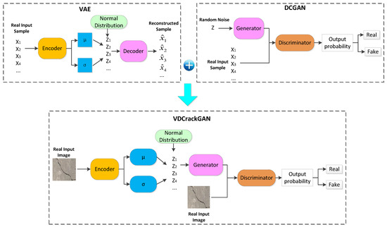
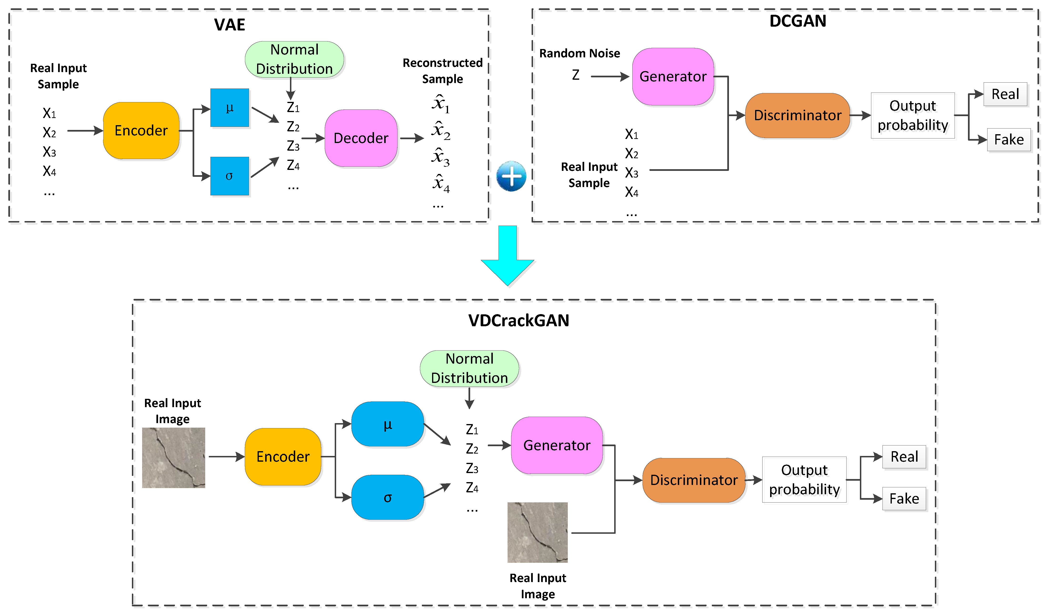
The structure of the generative network combining VAE and DCGAN is shown in Figure 1. The network consists of three parts: encoder; generator (also known as decoder); and discriminator. The encoder encodes the real road crack images in the training dataset, maps the crack images to the latent space, extracts the relevant feature information of the real road crack images, and outputs the mean and variance of the Gaussian distribution obeyed by the latent variables corresponding to the real sample vector. Subsequently, the latent variables are obtained by random sampling based on this Gaussian distribution. The generator (decoder) utilizes the latent variables as input and generates the corresponding crack images. Lastly, the discriminator discriminates the crack images generated by the generator and the real road crack images and outputs the probability value of an image being a real road crack.

Figure 1. The Network Architecture of VDCrackGAN.

3.1.1. Encoder

In this paper, the classic ResNet18 is employed directly as the encoder part, with the fully connected layer for classification subsequently removed. The specific network composition is shown in Table 1. Since the ResBlock module of ResNet18 is already well known to researchers, this paper does not delve into its details. For details, please refer to Reference [31]. In this study, the input image size is 256 × 256, and the output feature map is 8 × 8 after five downsamplings. Then, through the adaptive average pooling layer, the 1 × 1 feature output with 512 channels is obtained.

Table 1. Encoder Network Architecture.

Layer	Type	Filter Size	Stride	Out Channels	Feature Map Size	Activation
1	Conv	7 × 7	2	64	128 × 128	ReLu
2	Maxpool	3 × 3	2	64	64 × 64	ReLu
3	ResBlock1	3 × 3	1	64	64 × 64	ReLu
4	ResBlock2	3 × 3	2	128	32 × 32	ReLu
5	ResBlock3	3 × 3	2	256	16 × 16	ReLu
6	ResBlock4	3 × 3	2	512	8 × 8	ReLu
7	avgpool			512	1 × 1
8	fc(μ) *			100
9	fc(σ) *			100

* The fc layers of Layer 8 and Layer 9 are not serial but parallel after adaptive average pool layer. They output the mean μ and variance σ with 100 channels, respectively, which is also the commonly used number of channels of latent variable z.

Subsequently, through two fully connected layers, the mean and variance are outputs, respectively, which are the mean and variance of the Gaussian distribution of the latent variable corresponding to the true sample vector.

It is worth mentioning that the latent variable z is not sampled directly from the N (μ, σ) distribution. This is because it could lead to difficulties in calculating the backpropagation gradient due to the high variance. The specific approach is to set a differentiable transformation z = μ + ε × σ, where the noise variable ε is distributed according to N (0,1). The original direct sampling from N (μ, σ) is changed to sampling from N (0,1), and then, z = μ + ε × σ is calculated to obtain z. In this way, the derivation of z is transformed into the derivation of μ and σ, which solves the backpropagation problem.

3.1.2. Generator

The generator is mainly composed of a stack of multiple deconvolutional layers (also known as transposed convolutional layers). The input vector is the encoder’s output, Z, where the number of channels is usually set to 100. The generator needs to undergo 6 deconvolutional upsamplings with a stride of 2, ultimately producing a 256 × 256 crack image with 3 channels. The last deconvolutional layer of the generator employs the Tanh activation function, and the other layers use the ReLU activation function. The details of each network layer are shown in Table 2.

Table 2. Generator Network Architecture.

Layer	Type	Filter Size	Stride	Out Channels	Feature Map Size	Activation
1	Deconv	4 × 4	1	512	4 × 4	ReLU
2	Deconv	4 × 4	2	384	8 × 8	ReLU
3	Deconv	4 × 4	2	256	16 × 16	ReLU
4	Deconv	4 × 4	2	192	32 × 32	ReLU
5	Deconv	4 × 4	2	96	64 × 64	ReLU
6	Deconv	4 × 4	2	64	128 × 128	ReLU
7	Swin Transformer Block	—	—	—	128 × 128	—
8	Deconv	4 × 4	2	3	256 × 256	Tanh

3.1.3. Discriminator Network Architecture

The discriminator is also composed of multiple convolutional layers stacked together, similar to common image classification networks, as illustrated in Table 3. The input layer receives the raw image data, with the input dimension typically being (Batch_size, 3, H, W). The middle layers gradually reduce the feature map size from H×W to H/64 × W/64 through six convolution operations, each with a stride of 2. All convolution kernels employed are of size 4 × 4. The Sigmoid activation function is used for the last layer of the discriminator, and leakyReLU is used for other layers. The last convolutional layer converts the output into a 1-channel feature value, which is then passed through the Sigmoid function to produce a probability value of the input data being a real image.

Table 3. Discriminator Network Architecture.

Layer	Type	Filter Size	Stride	Out Channels	Feature Map Size	Activation
1	Conv	4 × 4	2	64	128 × 128	LeakyReLU
2	Conv	4 × 4	2	128	64 × 64	LeakyReLU
3	Conv	4 × 4	2	256	32 × 32	LeakyReLU
4	Conv	4 × 4	2	384	16 × 16	LeakyReLU
5	Conv	4 × 4	2	512	8 × 8	LeakyReLU
6	Conv	4 × 4	2	768	4 × 4	LeakyReLU
7	Conv	4 × 4	1	1	1 × 1	Sigmoid

3.2. Loss Function

3.2.1. Loss Function of VAE

As shown in Figure 1, VAE consists of two parts: encoder and decoder. The encoder is responsible for converting data samples x into latent representation z, while the decoder’s function is decoding the latent representation z back to the data space. It can be expressed as

$$z\sim Enc(x)=q(z\left|x\right.),\hspace{1em}\tilde{x}\sim Dec(z)=p(x\left|z\right.)$$

(1)

VAE regularizes the encoder by imposing a prior on the latent distribution p(z). z is usually chosen to follow the N (0, 1) distribution. The VAE loss is minus the sum of the expected log likelihood (the reconstruction error) and a prior regularization term [8]:

$$L_{VAE}=-E_{q(z\left|x\right.)}\left[\log {\displaystyle \frac{p(x\left|z\right.)p(z)}{q(z\left|x\right.)}}\right]=L_{llike}^{pixel}+L_{prior}$$

(2)

where $L_{llike}^{pixel}$ is the pixel reconstruction loss, and $L_{prior}$ is the prior regularization loss, i.e., KL divergence, which can be expressed as

$$L_{llike}^{pixel}=-E_{q(z\left|x\right.)}[\log p(x\left|z\right.)]$$

(3)

$$L_{prior}=D_{KL}(q(z\left|x\right.)‖p(z))$$

(4)

Reconstruction loss is used to measure the difference between the samples generated by the decoder and the real data and is commonly used as the mean square error (MSE). The mean square error evaluates the reconstruction quality by calculating the pixel difference between the reconstructed and real samples. However, the issue is that the mean square error, as a pixel-level difference metric, does not correspond to human visual perception. For example, a small image translation may bring a huge pixel difference (mean square error), while human vision does not notice this change at all. This limitation will be optimized and improved in the loss function of VDCrackGAN.

3.2.2. Loss Function of VDCrackGAN

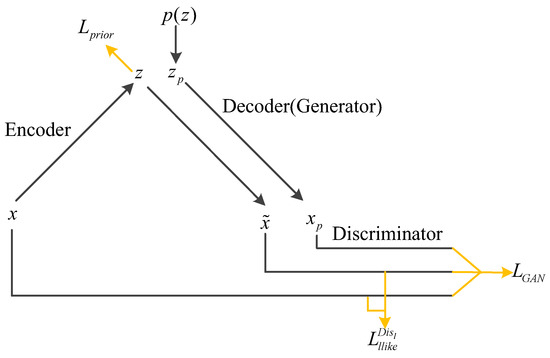
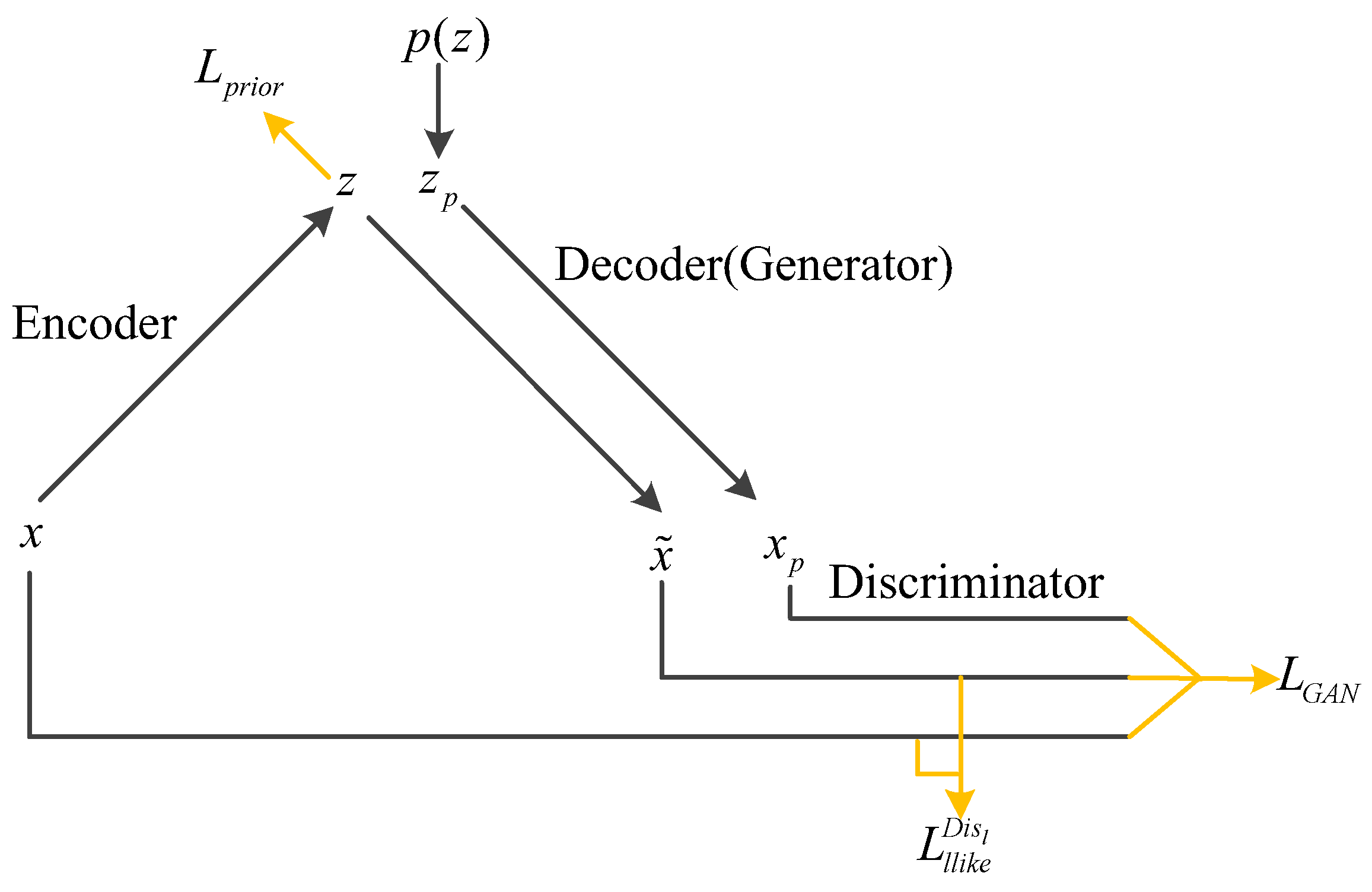
Since the pixel-wise reconstruction error is not very suitable for images, high-level feature matching loss will be used to optimize this problem in VDCrackGAN. The high-level feature matching loss function computes the difference between the generated image and the real image in the high-level feature space. It can not only measure the image similarity but also has sufficient invariance. Figure 2 is an information flow diagram for VDCrackGAN training, and this diagram is used to illustrate the composition of the VDCrackGAN loss function.

Figure 2. The information flow for VDCrackGAN training [8].

The total loss function consists of 3 terms:

$$L=L_{prior}+L_{llike}^{Di{s}_l}+L_{GAN}$$

(5)

The first item is the prior loss of the latent variable z, which is the KL loss of VAE, as shown in Equation (4). The second term is the high-level feature matching loss, which is used to replace the pixel reconstruction loss. The features are extracted in the discriminator. Assuming that it is in the lth layer of the discriminator, the feature matching loss can be expressed as

$$L_{llike}^{Di{s}_l}=-E_{q(z\left|x\right.)}[\log p(Di{s}_l(x)\left|z\right.)]$$

(6)

The third item is the discriminator loss of GAN that we are familiar with, expressed as

$$L_{GAN}=\log (Dis(x))+\log (1-Dis(\tilde{x}))+\log (1-Dis(x_p))$$

(7)

In order to study the impact of the three loss weights on model training, we actually added a weight term to the total loss:

$$L={\lambda }_p\times L_{prior}+{\lambda }_{\mathrm{l}}\times L_{llike}^{Di{s}_l}+{\lambda }_G\times L_{GAN}$$

(8)

3.3. Further Network Optimization

To further optimize the network, spectral normalization and Swin Transformer are introduced. Spectral normalization greatly improves the stability of network training, and Swin Transformer significantly improves the quality of samples generated by the network.

3.3.1. Spectral Normalization

Traditional GAN networks often suffer from the issue of low training stability. To tackle the problem of GAN training stability, WGAN directly restricts the elements in the parameter matrix, ensuring they do not exceed a certain value. Although this method can guarantee the Lipschitz constraint, it unfortunately destroys the parameter matrix structure. To address this problem, Takeru Miyato et al. [11] proposed a method that satisfied the Lipschitz condition without destroying the matrix structure, namely, spectral normalization (SN), and applied it to GAN. They found that by normalizing the weight matrix in the discriminator to the corresponding spectral norm, the Lipschitz constant of the discriminator can be effectively controlled, helping GAN to be more stable during training and improving its generalization performance.

The core idea of spectral normalization is to divide the network parameters of each layer by the spectral norm of the parameter matrix to achieve the condition that Lipschitz is equal to 1, which can be expressed as

$${\overline{W}}_{SN}(W):={\displaystyle \frac{W}{\sigma (W)}}$$

(9)

where σ(W) is the spectral norm of the matrix W (L2 matrix norm of W).

3.3.2. Swin Transformer

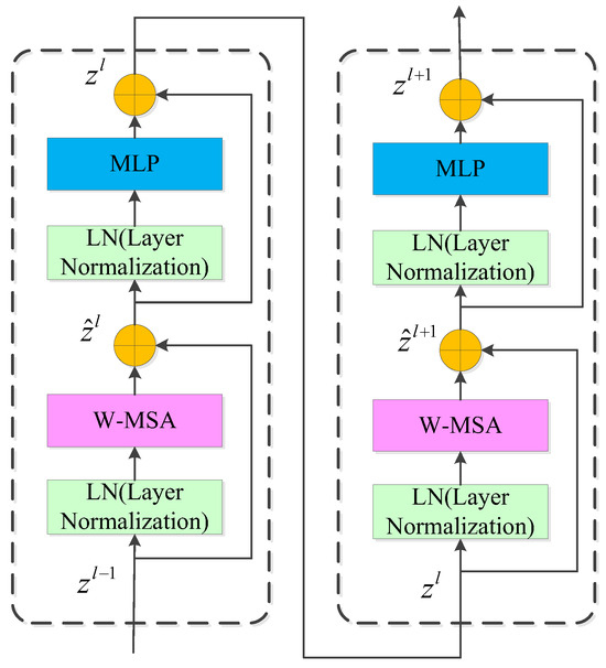
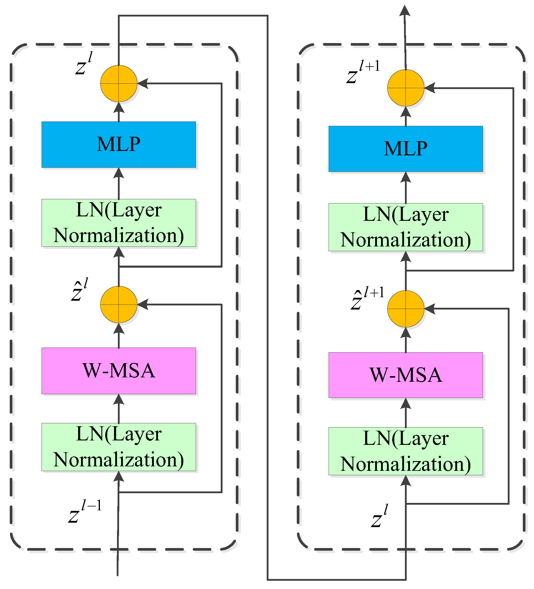
The Transformer model has been widely used in the field of computer vision due to its powerful feature extraction capability based on the self-attention mechanism. Liu et al. [9] proposed the Swin Transformer model, which is a Transformer model based on the window attention mechanism and can more flexibly capture feature information of different types and scales. The model divides the input image into windows of different sizes and independently calculates the attention weight on each window, thereby achieving flexible processing of features of different scales. This paper introduces the core component of the Swin Transformer, the Swin Transformer Block, and combines it with CNN to improve the performance of the generative adversarial network. The main composition of this component is shown in Figure 3. Compared with ViT Transformer, Swin Transformer replaces the standard multi-head self-attention module (MSA) with a window-based multi-head self-attention module (W-MSA) or a shifted window-based multi-head self-attention module (SW-MSA), while keeping other parts unchanged. As shown in Figure 3, the Swin Transformer module typically uses two modules together in succession, the former using W-MSA and the latter using SW-MSA. The stack of two Swin Transformer Blocks can be expressed as

$$\begin{array}{c}{\widehat{z}}^l=\mathit{W-MSA}(LN(z^{l-1}))+z^{l-1}\\ z^l=MLP(LN({\widehat{z}}^l))+{\widehat{z}}^l\\ {\widehat{z}}^{l+1}=\mathit{SW-MSA}(LN(z^l))+z^l\\ z^{l+1}=MLP(LN({\widehat{z}}^{l+1}))+{\widehat{z}}^{l+1}\end{array}$$

(10)

Figure 3. Two stacked Swin Transformer Blocks [9].

4. Experiment

4.1. Evaluation Metrics

This paper utilizes two common metrics for evaluating the performance of generative adversarial networks, Inception Score (IS) and Fréchet Inception Distance (FID), to evaluate the experimental results.

IS is an indicator based on the Inception network, which evaluates the quality of the generated samples by calculating the entropy of the output probability distribution of the generated image in the Inception network. Generally, a higher IS score signifies better quality of the generated samples.

FID, on the other hand, is an indicator based on the Fréchet distance employed to quantify the similarity between the generated image and the real image. It evaluates the quality of the generated samples by calculating the Fréchet distance between the feature distribution of the generated image and the real image in the Inception network. Usually, a lower FID indicates superior quality of the generated samples.

4.2. Dataset and Experimental Environment

The training dataset used in the experiment is Concrete Crack Images for Classification [32]. The software and hardware environment of the experiment is shown in Table 4. The settings of hyperparameters included the following: the basic learning rate was set to 0.0002; the batch size was set to 32; and the optimizer was Adam with betas (0.5, 0.999).

Table 4. Experiment environment.

Type	Configuration
CPU	Intel i9-10900X 3.7 GHz
GPU	NVIDIA GeForce RTX 3090 24 GB
RAM	DDR4 3000 MHz 64 GB
Soft	Python 3.7.6, Pytorch 1.9.0, Cuda 11.3

4.3. Experiment Results

4.3.1. Model Comparison Experiment

To verify the effectiveness of the method proposed in this paper, model comparison experiments were carried out, and the experimental results are shown in Table 5. The experimental data show that the VAE-DCGAN model, which combines VAE with DCGAN, improves the IS score and FID score by 8% and 11.2% over the original DCGAN model, respectively. The introduction of spectral normalization is effective. The IS score and FID score of the VAE-DCGAN+SN model are improved by 1.3% and 1.8%, respectively, compared with the VAE-DCGAN model, and by 9.7% and 12.8%, respectively, compared with DCGAN. Finally, the introduction of the Swin Transformer is also effective, again improving the IS score and FID score by 2.8% and 15.6% on top of VAE-DCGAN+SN, and the optimization improvement effect of this paper’s method on IS score and FID score reaches 13.6% and 26.4%, respectively, when compared to the original DCGAN. In addition, the IS and FID indicators of VDCrackGAN outperform those of SAGAN and WGAN in the crack generation task, as shown in Table 5. Moreover, the IS scores of the generated samples of VDcrackGAN are very close to the real crack samples, which also indicates the high quality of the generated crack images by VDcrackGAN.

Table 5. Comparison of different generative models.

Models	IS		FID
	Score	std	Score	std
real crack dataset	3.259	0.216	—	—
SAGAN	3.212	0.036	27.139	0.075
WGAN	3.176	0.048	38.762	0.092
DCGAN	2.923	0.037	36.414	0.085
VAE-DCGAN	3.106 (↑8.0 *)	0.046	32.331 (↑11.2)	0.081
VAE-DCGAN +SN	3.146 (↑9.7)	0.039	31.751 (↑12.8)	0.081
VAE-DCGAN +SN + Swin Transformer (our VDCrackGAN)	3.235 (↑13.6)	0.040	26.812 (↑26.4)	0.072

* The arrow ↑ represents the improvement in performance index, and the number after ↑ represents the percentage improvement in performance index relative to DCGAN.

4.3.2. Ablation Study

In order to obtain the optimal model, this paper mainly conducts ablation experiments on the position of the Swin Transformer module in the network layer of the generator network, the number of heads in the Swin Transformer’s multi-head attention, and the weight of each loss function in the weighted loss function.

The Influence of Different Swin Transformer Block Locations

Table 6 shows the comparison of IS and FID scores of crack image samples generated by VDCrackGAN, with the Swin Transformer Block located in different network layers. It can be found that the location of the Swin Transformer Block has an important influence on the model performance. When the Swin Transformer Block is located behind the 128 × 128 feature map (namely, feat128 in Table 6), it is obviously superior to other positions. The IS scores of feat128 are 2.3%, 0.7%, 8.0%, and 2.8% higher than that of feat64, feat32, feat16, and feat8, respectively, and it is very close to the IS score of the real crack dataset. Similarly, the FID score of feat128 is better than that of feat64, feat32, feat16, and feat8 by 42.2%, 28.2%, 56.0%, and 29.5%, respectively.

Table 6. Comparison of different Swin Transformer Block locations.

Position of Swin Transformer Block	IS		FID
	Score	std	Score	std
real crack dataset	3.259	0.216	—	—
feat128 1	3.235	0.040	26.812	0.072
feat64	3.162	0.038	46.410	0.097
feat32	3.214	0.046	37.333	0.086
feat16	2.995	0.033	60.955	0.091
feat8	3.148	0.038	38.033	0.083

¹ Feat128 represents the position of Swin Transformer Block located behind the feature map with the size of 128 × 128, that is, after layer 6 (as shown in Table 2), and so on.

The Influence of the Number of Heads in Swin Transformer’s Multi-Head Attention

Table 7 shows the influence of different head numbers of the Swin Transformer Block’s multi-head attention mechanism on the model performance. It can be found that when the head number is 4, the IS scores are 6.3% and 7.6% higher than when the head number is 8 and 16, respectively, and the FID score promotion percentages reach 42.2% and 45.8%, respectively.

Table 7. Comparison of different head numbers of Swin Transformer Block.

Num_Heads	IS		FID
	Score	std	Score	std
4	3.235	0.040	26.812	0.072
8	3.044	0.036	46.383	0.099
16	3.006	0.033	49.501	0.101

The Influence of the Weight of Each Loss Function

In this paper, the weighted loss function is used, and in order to study the influence of the weight of the loss function on the training results of the model, the related ablation experiments are also carried out. As shown in Equation (8), the weights of prior loss (KL loss) $L_{prior}$, feature matching loss $L_{llike}^{Di{s}_l}$, and discriminator loss $L_{GAN}$ are ${\lambda }_p$, ${\lambda }_{\mathrm{l}}$, and ${\lambda }_G$, respectively. Table 8 shows the influence of different weights on the training results. The optimal parameter group is 1.5 for ${\lambda }_p$, 0.01 for ${\lambda }_{\mathrm{l}}$, and 1.0 for ${\lambda }_G$.

Table 8. Comparison of different weights of loss functions.

Weight of Loss Function		IS		FID
		Score	std	Score	std
${\lambda }_p$	1	3.222	0.036	30.142	0.078
	1.5	3.235	0.040	26.812	0.072
	2	3.203	0.045	29.325	0.075
	3	3.112	0.037	37.858	0.087
	5	3.232	0.038	30.831	0.078
${\lambda }_{\mathrm{l}}$	0.01	3.235	0.040	26.812	0.072
	0.02	3.007	0.036	37.258	0.086
	0.05	2.893	0.042	73.874	0.130
${\lambda }_G$	1	3.235	0.040	26.812	0.072
	1.5	3.199	0.040	41.600	0.089
	2	3.144	0.039	43.460	0.094
	5	3.159	0.038	72.186	0.116

4.3.3. Crack Generating Effect

To further examine the generative effectiveness of VDCrackGAN, we conducted the following two comparative studies:

• We directly compared the human visual effects of the crack samples generated by VDCrakGAN with the real crack images;
• Crack samples generated by VDCrakGAN were used to train the image classification network to evaluate the effectiveness of VDCrakGAN for crack data augmentation.

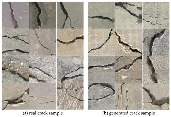
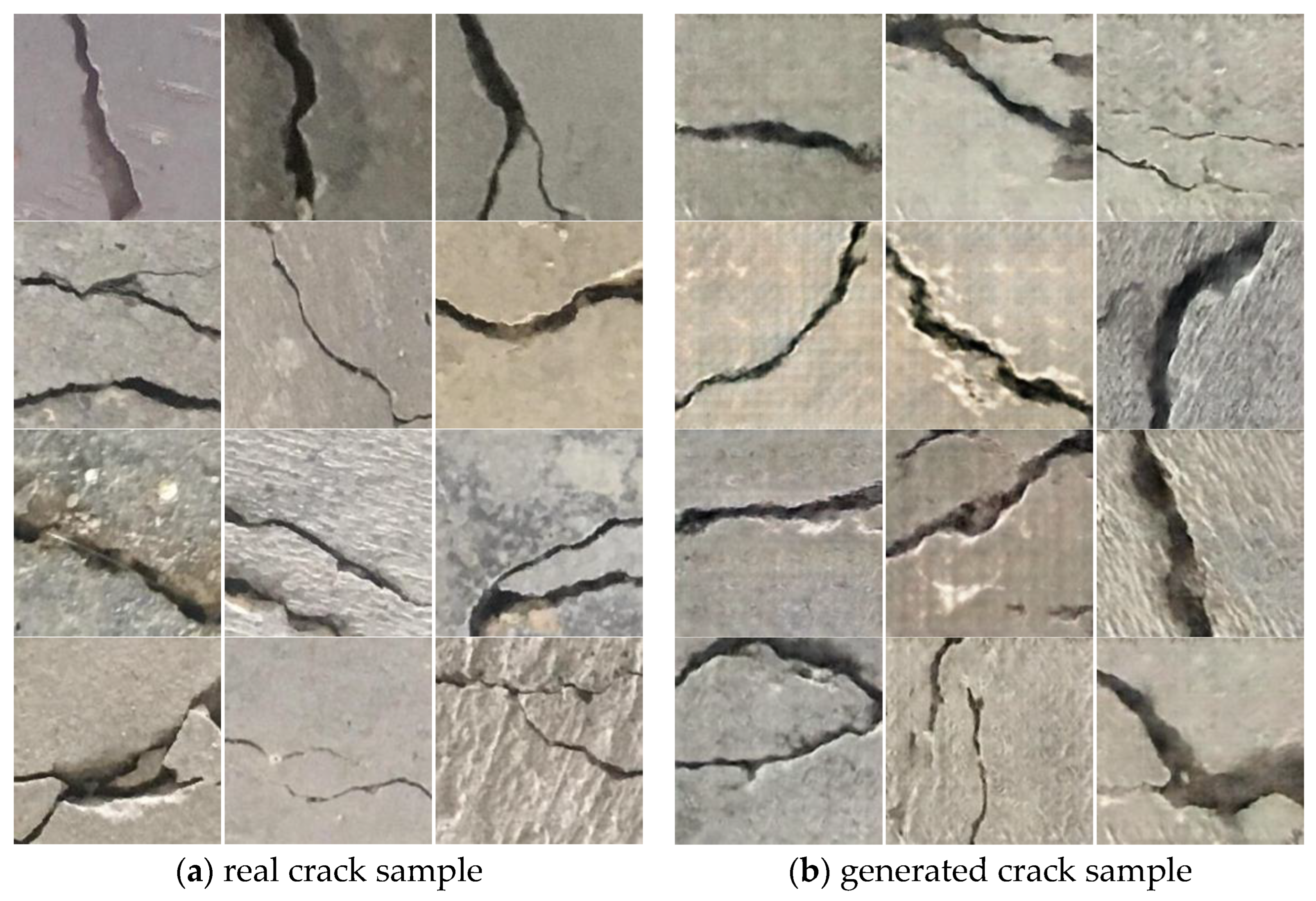
Figure 4 visualizes the effect of crack generation, with the left three columns displaying real crack samples and the right three columns showing generated crack samples by VDCrakGAN. As can be seen in the figure, the generated cracks are not only of high clarity but also of various morphologies, such as wide cracks, thin cracks, complex backgrounds, and intricate topologies. It is difficult to distinguish between the real cracks and the generated cracks only with the naked eye.

Figure 4. Human visual effect comparison of generated crack sample and real crack sample.

Furthermore, a classification experiment comparison between generated cracks and real cracks was conducted. The classic ResNet18 model was used for crack classification experiments. The experimental results are shown in Table 9. As can be seen from Table 9, augmenting the training set with generated crack samples can significantly improve the classification accuracy. Experiments 1, 2, and 3 show that when the original dataset is 500 real crack images, adding 1000 and 2000 generated cracks can improve the training outcomes by 0.9% and 1.6%, respectively. Similarly, experiments 4, 5, and 6 indicate that when the original dataset is 1000 real crack images, adding 1000 and 2000 generated cracks can improve the training results by 0.8% and 1.4%, respectively. In addition, the comparison between Experiments 2 and 4 reveals that adding 1000 generated cracks can achieve the same improvement effect as adding 500 real cracks and even slightly better. In summary, the generative network proposed in this paper proves effective for crack data augmentation.

Table 9. Effect of generated cracks for classification experiment.

Experiment No.	Training Dataset	Accuracy
1	500 real cracks	0.9583
2	500 real cracks + 1000 generated crack	0.9667
3	500 real cracks + 2000 generated cracks	0.9732
4	1000 real cracks	0.9655
5	1000 real cracks + 1000 generated crack	0.9735
6	1000 real cracks+ 2000 generated cracks	0.9788

5. Conclusions

In this paper, a VDCrackGAN network for crack generation was proposed by combining two classical generative models, VAE and DCGAN, and the network was further optimized by introducing spectral normalization and Swin Transformer. The IS and FID metrics of the crack samples generated using VDCrackGAN are improved by 13.6% and 26.4% compared with the original DCGAN. The results of generating crack samples for classification experiments also show that the generative network proposed in this paper is feasible for crack data augmentation. The crack generation in this paper is mainly used for crack classification and recognition, and crack generation in the fields of object detection and semantic segmentation will be carried out in the future.

References

- Zakeri, H.; Nejad, F.M.; Fahimifar, A. Image Based Techniques for Crack Detection, Classification and Quantification in As-phalt Pavement: A Review. Arch. Comput. Methods Eng. 2017, 24, 935–977. [Google Scholar] [CrossRef] [Scilit]
- Lecun, Y.; Bengio, Y.; Hinton, G. Deep Learning. Nature 2015, 521, 436–444. [Google Scholar] [CrossRef] [Scilit]
- Schmidhuber, J. Deep Learning in Neural Networks: An Overview. Neural Netw. 2015, 61, 85–117. [Google Scholar] [CrossRef] [Scilit] [PubMed]
- Cha, Y.J.; Choi, W.; Büyüköztürk, O. Deep Learning-Based Crack Damage Detection Using Convolutional Neural Networks. Comput. Civ. Infrastruct. Eng. 2017, 32, 361–378. [Google Scholar] [CrossRef] [Scilit]
- Zou, Q.; Zhang, Z.; Li, Q.; Qi, X.; Wang, Q.; Wang, S. DeepCrack: Learning Hierarchical Convolutional Features for Crack Detection. IEEE Trans. Image Process. 2019, 28, 1498–1512. [Google Scholar] [CrossRef] [Scilit]
- Doersch, C. Tutorial on Variational Autoencoders. arXiv 2016, arXiv:1606.05908. [Google Scholar]
- Goodfellow, I.; Pouget-Abadie, J.; Mirza, M.; Xu, B.; Warde-Farley, D.; Ozair, S.; Courville, A.; Bengio, Y. Generative Adversarial Networks. Commun. ACM 2020, 63, 139–144. [Google Scholar] [CrossRef] [Scilit]
- Larsen, A.B.L.; Sønderby, S.K.; Larochelle, H.; Winther, O. Autoencoding beyond Pixels Using a Learned Similarity Metric. In Proceedings of the 33rd International Conference on Machine Learning, ICML 2016, New York City, NY, USA, 19–24 June 2016; Volume 4, pp. 2341–2349. [Google Scholar]
- Liu, Z.; Lin, Y.; Cao, Y.; Hu, H.; Wei, Y.; Zhang, Z.; Lin, S.; Guo, B. Swin Transformer: Hierarchical Vision Transformer Using Shifted Windows. In Proceedings of the IEEE/CVF International Conference on Computer Vision (ICCV), Montreal, BC, Canada, 11–17 October 2021; pp. 9992–10002. [Google Scholar] [CrossRef] [Scilit]
- Radford, A.; Metz, L.; Chintala, S. Unsupervised Representation Learning with Deep Convolutional Generative Adversarial Networks. In Proceedings of the 4th International Conference on Learning Representations, ICLR 2016-Conference Track Proceedings, San Juan, Puerto Rico, 2–4 May 2016; pp. 1–16. [Google Scholar]
- Miyato, T.; Kataoka, T.; Koyama, M.; Yoshida, Y. Spectral Normalization for Generative Adversarial Networks. In Proceedings of the 6th International Conference on Learning Representations, ICLR 2018-Conference Track Proceedings, Vancouver, BC, Canada, 30 April–3 May 2018. [Google Scholar]
- Yu, X.; Wu, X.; Luo, C.; Ren, P. Deep Learning in Remote Sensing Scene Classification: A Data Augmentation Enhanced Convolutional Neural Network Framework. GIScience Remote Sens. 2017, 54, 741–758. [Google Scholar] [CrossRef] [Scilit]
- González, R.E.; Muñoz, R.P.; Hernández, C.A. Galaxy Detection and Identification Using Deep Learning and Data Augmentation. Astron. Comput. 2018, 25, 103–109. [Google Scholar] [CrossRef] [Scilit]
- Huang, H.; Li, Q.; Zhang, D. Deep Learning Based Image Recognition for Crack and Leakage Defects of Metro Shield Tunnel. Tunn. Undergr. Space Technol. 2018, 77, 166–176. [Google Scholar] [CrossRef] [Scilit]
- Zhang, H.; Cisse, M.; Dauphin, Y.N.; Lopez-paz, D. Mixup: Beyond Empirical Risk Minimization. arXiv 2017, arXiv:1710.09412. [Google Scholar]
- Devries, T.; Taylor, G.W. Improved Regularization of Convolutional Neural Networks with Cutout. arXiv 2017, arXiv:1708.04552. [Google Scholar]
- Yun, S. CutMix: Regularization Strategy to Train Strong Classifiers with Localizable Features. In Proceedings of the 2019 IEEE/CVF International Conference on Computer Vision (ICCV), Seoul, Republic of Korea, 27 October–2 November 2019; pp. 6022–6031. [Google Scholar] [CrossRef] [Scilit]
- Diaz-Pinto, A.; Colomer, A.; Naranjo, V.; Morales, S.; Xu, Y.; Frangi, A.F. Retinal Image Synthesis and Semi-Supervised Learning for Glaucoma Assessment. IEEE Trans. Med. Imaging 2019, 38, 2211–2218. [Google Scholar] [CrossRef] [Scilit] [PubMed]
- Chen, J.; Song, W. GAN-VAE: Elevate Generative Ineffective Image Through Variational Autoencoder. In Proceedings of the 2022 5th International Conference on Pattern Recognition and Artificial Intelligence, PRAI 2022, Chengdu, China, 19–21 August 2022; pp. 765–770. [Google Scholar] [CrossRef] [Scilit]
- Mirza, M.; Osindero, S. Conditional Generative Adversarial Nets. arXiv 2014, arXiv:1411.1784. [Google Scholar]
- Arjovsky, M.; Chintala, S.; Bottou, L. Wasserstein GAN. arXiv 2017, arXiv:1701.07875. [Google Scholar]
- Gulrajani, I.; Ahmed, F.; Arjovsky, M.; Dumoulin, V.; Courville, A. Improved Training of Wasserstein GANs. Adv. Neural Inf. Process. Syst. 2017, 30, 5768–5778. [Google Scholar]
- Zhu, J.; Park, T.; Efros, A.A.; Ai, B.; Berkeley, U.C. Unpaired Image-to-Image Translation Using Cycle-Consistent Adversarial Networks. In Proceedings of the 2017 IEEE International Conference on Computer Vision (ICCV), Venice, Italy, 22–29 October 2017; pp. 2242–2251. [Google Scholar] [CrossRef] [Scilit]
- Zhang, H.; Goodfellow, I.; Metaxas, D.; Odena, A. Self-Attention Generative Adversarial Networks. In Proceedings of the 36th International Conference on Machine Learning, ICML 2019, Long Beach, CA, USA, 9–15 June 2019; pp. 12744–12753. [Google Scholar]
- Chen, G.; Teng, S.; Lin, M.; Yang, X.; Sun, X. Crack Detection Based on Generative Adversarial Networks and Deep Learning. KSCE J. Civ. Eng. 2022, 26, 1803–1816. [Google Scholar] [CrossRef] [Scilit]
- Ma, D.; Fang, H.; Wang, N.; Zhang, C.; Dong, J.; Hu, H. Automatic Detection and Counting System for Pavement Cracks Based on PCGAN and YOLO-MF. IEEE Trans. Intell. Transp. Syst. 2022, 23, 22166–22178. [Google Scholar] [CrossRef] [Scilit]
- Hou, Y.; Liu, S.; Cao, D.; Peng, B.; Liu, Z.; Sun, W.; Chen, N. A Deep Learning Method for Pavement Crack Identification Based on Limited Field Images. IEEE Trans. Intell. Transp. Syst. 2022, 23, 22156–22165. [Google Scholar] [CrossRef] [Scilit]
- Maeda, H.; Kashiyama, T.; Sekimoto, Y.; Seto, T.; Omata, H. Generative Adversarial Network for Road Damage Detection. Comput.-Aided Civ. Infrastruct. Eng. 2021, 36, 47–60. [Google Scholar] [CrossRef] [Scilit]
- Jin, T.; Ye, X.W.; Li, Z.X. Establishment and Evaluation of Conditional GAN-Based Image Dataset for Semantic Segmentation of Structural Cracks. Eng. Struct. 2023, 285, 116058. [Google Scholar] [CrossRef] [Scilit]
- Zhang, X.; Peng, B.; Al-Huda, Z.; Zhai, D. FeatureGAN: Combining GAN and Autoencoder for Pavement Crack Image Data Augmentations. Int. J. Image Graph. Signal Process. 2022, 14, 28–43. [Google Scholar] [CrossRef] [Scilit]
- He, K.; Zhang, X.; Ren, S.; Sun, J. Deep Residual Learning for Image Recognition. In Proceedings of the 2016 IEEE Conference on Computer Vision and Pattern Recognition (CVPR), Las Vegas, NV, USA, 27–30 June 2016. [Google Scholar]
- Zhang, L.; Yang, F.; Daniel Zhang, Y.; Zhu, Y.J. Road Crack Detection Using Deep Convolutional Neural Network. In Proceedings of the 2016 IEEE International Conference on Image Processing (ICIP), Phoenix, AZ, USA, 25–28 September 2016; pp. 3708–3712. [Google Scholar] [CrossRef] [Scilit]
Disclaimer/Publisher’s Note: The statements, opinions and data contained in all publications are solely those of the individual author(s) and contributor(s) and not of MDPI and/or the editor(s). MDPI and/or the editor(s) disclaim responsibility for any injury to people or property resulting from any ideas, methods, instructions or products referred to in the content. |
© 2024 by the authors. Licensee MDPI, Basel, Switzerland. This article is an open access article distributed under the terms and conditions of the Creative Commons Attribution (CC BY) license (https://creativecommons.org/licenses/by/4.0/).