


Abstract
Adjacency matrix visualization is a common method for presenting graph data, and the Focus+Context technique can be used to explore the details of the ROI (region of interest). Embedded views and multi-view approaches are usually applied when locating and comparing attributes among multiple nodes. However, the embedded view has an issue of edge occlusion, while the multi-view would cause repeated perspective switching. In this paper, we propose a Multivariate Fence (MVF) model as a focus view of the adjacency matrix to locate and compare attributes among nodes. An additional spatial parallel coordinate is added to the 2D adjacency matrix in an immersive environment so that the attribute information can be shown in a single view without blocking edge information. We also conduct a user study to evaluate the performance of the MVF. The results show that the MVF has better efficiency and accuracy in locating and comparing the multivariate adjacency matrix in the immersive environment against the existing focus model. Moreover, the MVF model is easier to understand and is preferred by users.
1. Introduction
In graph visualization, the adjacency matrix is a commonly used method that expresses the relationship between N nodes through an N × N matrix [1]. Multivariate node attributes are also important information in the adjacency matrix. Still, little space is left for attributes display because the adjacency matrix expresses whether the relationship exists between two nodes and makes vital information in conspicuous [2]. The Focus+Context (F+C) technique is used to solve this issue.
The F+C technique displays node attributes mainly by using the embedded view and multi-view method [3,4]. In the embedded view [5,6], the attributes of the corresponding two nodes are superimposed on the edge of the focus, which will lead to the occlusion of edge information (such as color mapping). The multi-view [3,7] changes the encoding of the focus area for attribute displacement so that the original edge information will be covered entirely. Hence, the analyst has to constantly switch between the two views in the process of data analysis [6,7]. Therefore, showing edge and node attributes without occlusion is challenging in the traditional F+C focus view.
An immersive environment can be led by Virtual/Augmented/Mixed Reality, wall-size displays, and tabletops [8]. A survey of Immersive Analytics [9] reports that 3D graphics, stereo vision, and head tracking are the necessary components that should be provided in this environment. The application of immersive environments in data visualization has become a new data analysis technology [10]. Compared with the 2D view, it adds depth to increase the display space and provides new possibilities for display mode and layout [11]. In addition, new interaction methods offer a new interactive experience and help users explore data more naturally and coherently.
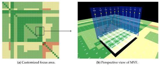
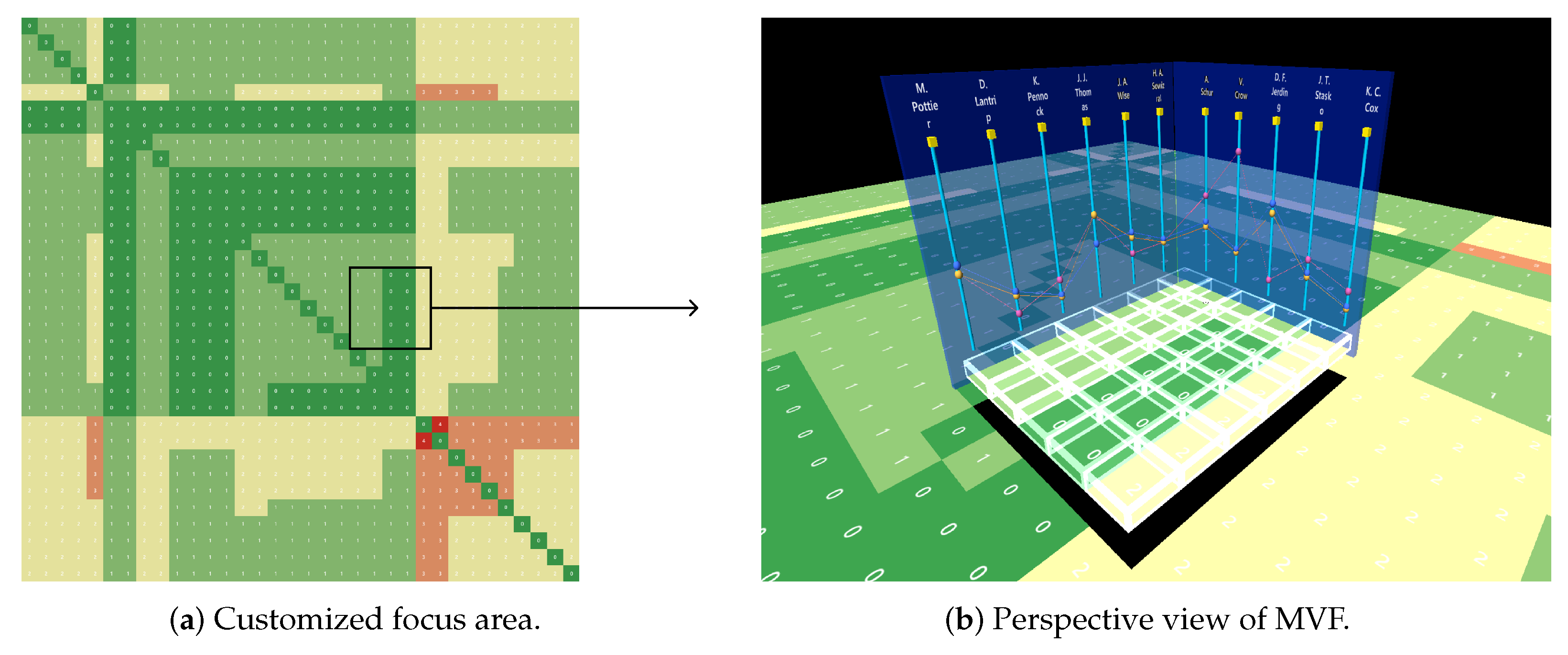
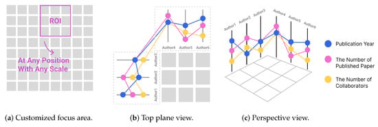
Therefore, we propose a focus view model named Multivariate Fence (MVF), which uses the spatial parallel coordinate in the immersive environment to display node attributes. The MVF (Figure 1), together with the focus area, constitutes a focus data analysis workspace, which displays all information of nodes and edges simultaneously without blocking edges. This method improves the efficiency and accuracy of locating and comparing attributes between nodes and enhances the understanding of the relationship between nodes and edges of the adjacency matrix. We also conducted a controlled experiment to evaluate the performance of the MVF.
Figure 1.
Multivariate Fence—A focus view model for adjacency matrix showing node attributes.
This work contributes the following: (1) a visualization model for visualizing multidimensional properties of graph data using an immersive environment; (2) a visualization method for locating and comparing adjacency matrix nodes in an immersive environment; and (3) a VR-based prototype system for visualizing high-dimensional graph data and an evaluation.
2. Related Work
2.1. Interactions in Adjacency Matrix
Three main interaction techniques are used to explore the adjacency matrix [12]: Focus+Context, Overview+Detail, and Pan&Zoom. Focus+Context technology distorts the information space; Overview+Details requires additional view assistance to display information and user effort to correlate the two; and Pan&Zoom results in higher working memory because the user can see only one view at a time.
Focus+Context comes in two major forms: lens and fold. The lens usually emphasizes the contents of an area using magnification, such as suppressing scattered information, showing details, and changing mappings. PaperLens [13] uses square hardware as a lens to transform the view of the covered area, and the size of the lens coverage area is relatively fixed. RMC [6] solves this problem by scaling the lens view transformation area. BodyLens [14], SpiderEye [15], and ShadowTouch [16] use lenses with different shapes (round, rectangular, humanoid outline) to change the view mapping to show details, and can adjust the size of the covered area. However, the above directly overwrites the original view due to insufficient display space, resulting in information loss. Melang [17] is a 3D distortion technology that folds the uninterested part to the rear to reduce the display area. Similarly, SpaceFold [18] and Multi-touch document folding [19,20] support multiple focal points to be displayed at the same time. Still, the focus shape is relatively fixed, the number of focal points is limited, the deformation is more serious, and more information is lost.
Overview+Details comes in three major forms: mini-maps, different views from different perspectives, and view slices. A mini-map is a small map of the whole world, providing an overview of the user and the relationship between the details and the entire world. Different views from different perspectives are used to display details of new areas through other views. MARVIS [21] displays node attributes in the figure as bar charts beside the Overview area. View slicing extracts part of the global view as details and zooms in to display. Visualizing Dynamic Networks [22] uses this method to show details of the matrix cube. This interaction technique can take up limited view space or require the new view presentation space to be expanded.
Pan&Zoom technology includes geometric and semantic zooming. The former specifies the scale of the enlarged spatial scales, while the latter changes the level of detail by changing the visual code. Van Wijk and Nuij summarized smooth and efficient geometric zooming and panning techniques and presented a model to calculate a solution for optimal-view animations [12,23]. ZAME [5] and TimeMatrix [24] are content-aware technologies that rely on semantic zooming to display different encoding details based on the scale level. Semantic scaling is also included in RMC [6], where four levels of details (LOD) are designed based on the scale level. Pan&Zoom technology provides users with more multivariate information through zoom operation.
This work mainly aims to improve the problems of space limitation and occlusion, display multiple attributes of nodes without blocking the region of interest (ROI), and support more free zooming.
2.2. ROI Presentation Techniques of Adjacency Matrix
We investigate three methods of visualizing multiple attributes of the adjacency matrix when selecting the ROI. They are embedded view, multi-view, and juxtaposed view.
The embedded view usually encodes multiple attributes on edges, which can be embedded into the unit cell (for one edge/two nodes) and meta cells (for cluster). When embedding in the unit cell, due to the small area allocated by the adjacency matrix to each cell, multi-attribute does not have sufficient display room and will block edge coding, which makes it difficult for users to observe. For meta cells, ZAME [5] calculates the attribute values to obtain the final color map, which loses many details. RMC [6] justifies all the attribute information on the edge, making the positional relationship among attributes, nodes, and edges challenging to understand.
Multi-view uses an auxiliary view to display multivariate, which solves the problem of insufficient display room in the adjacency matrix. Visualization in GraSp [3] uses mobile devices to display graphs on a large display. Although it expands the new display space, it requires frequent view switching when mapping between two graphs. The multi-view technique can also be completed by view switching, completely covering the original visual information and requiring frequent page switching to complete the task. These conditions all lead to user fatigue. Multi-view may also need to be accessed through multiple software, which not only causes window switching but also increases software installation requirements that is not convenient.
The juxtaposed view displays multiple attributes by placing different encoding views at the side of the original view. This method does not affect the encoding of the original view. However, it is not easy to match specific items [25]. As a result, of the limited display area this technique needs interaction widgets such as sliders for auxiliary observation, or requires the user to switch the view back and forth. For example, Matrix Zoom [26] provides views of different encoding. Some views need scroll-view [27,28,29] to show complete content, which is hard to match items. Hence, the interaction process is cumbersome.
In this work, we place the multivariate information on the side of the ROI to make the relationship among attributes, nodes, and edges more intuitive and use spatial dimensions to display information without blocking any mapping codes in the original view.
2.3. Immersive Analytics
Immersive Analytics (IA) was defined in 2015 as “the applicability and development of emerging user interface technologies for creating more engaging and immersive experiences and seamless workflows for data analysis applications” and more recently as “the use of engaging, embodied analysis tools to support data understanding and decision making” [10]. A recent survey by Fonnet et al. [9] provides an extensive overview of IA. The visual analysis of multi-dimensional data in immersive environment consists of four aspects: immersive visualization, multi-dimensional data, ultimate space, and interaction input. We summarize each in the following paragraphs.
Immersive visualization. Immersive visualization is an engaging, multi-sensory, and embodied analysis tool to support exploration, communication reasoning, and decision making. Recent advances in immersive technologies (VR, AR, MR, large display, tangible surfaces, etc.) show new opportunities to analyze, explore, and present data using these technologies [30]. It has been applied to applications such as information visualization and image immersion. It has proven effective in many other scientific applications, such as brain tumor analysis, archaeology, geographic information systems, geosciences, and physics [31]. Immersion technology provides a broader space, changes the traditional windows, icons, menus, pointer (WIMP) interaction paradigm, and provides a new interactive experience.
Multidimensional data. Analyzing multidimensional datasets to find insights and trends has been a popular topic within IA. Several visualization tools and case studies have emerged. DXR [32], ImAxes [31], IATK [33], and other tools that support multi-dimensional data rendering in immersive environments. In a case study, MARVIS [21] combined AR and mobile devices to display more data dimensions in different views in space, providing more possibilities for view combination. Personal Augmented uses large displays to combine with AR and proposes a design space suitable for multi-person collaborative data analysis. For example, Liu et al. [34] found that users were faster and more accurate when using a flat layout with a small number of multiples. Still, as multiples increased, a half-circle layout provided the best performance. The visual layout is relatively fixed in the above cases, and the space is not fully utilized.
Ultimate space. DataHop [35] and Maps Around Me [36] have a higher degree of expansion and utilization of space. Maps Around Me expands multiple hierarchies of map data in a spherical layout and provides an automatic layout technique to help users quickly organize data locations. DataHop uses the process of user data exploration as the layout, which can not only expand the space of data display; but also record the process of user exploration. However, one can easily get lost in that environment.
Interaction input. IA changes the traditional input, abandoning the WIMP paradigm, usually using new input methods such as air gestures and head rotation. Regarding navigation, devices with six degrees of freedom (6DOF) can recognize the movement of characters in space and support users to walk and observe directly. Other ways, such as teleportation, can be used to facilitate quick movement in large spaces. Gesture interaction technology is also maturing. One paper studied the effect of different input methods on low-level tasks in a 3D node-link graph [37,38], and the results showed no effect on accuracy. Still, for complex graphs, gestures were significantly faster. Immersive interactive environments also have limitations, such as color distortion, perspective, and occlusion, which must be explored and solved.
At present, VR is a relatively mature technology among interactive devices that can provide an immersive environment with a reasonably good effect on display resolution and color. Therefore, VR is adopted in this project to provide an immersive environment, and gesture interaction is used to provide a new way of natural interaction.
2.4. Parallel Coordinate Plot
Parallel Coordinate Plot (PCP) is a multidimensional data visualization technique [39], which can arrange multiple attributes in parallel on a 2D plane. Parallel axes are usually used to represent attributes, and the location of data items on the axis helps in understanding the distribution interval of the attribute [40] and identify outliers. Through line patterns in PCP, such as tilt degree and density, the relationship between clusters of data items, adjacent attributes, and correlation can be perceived easily.
PCP allows users to understand an overview of the data, but representing a large amount of data can cause overdrawn links. At present, many ways are applied to solve this problem, such as using a clustering algorithm [41,42] and adding another visual coding [40,43].
We change the traditional mapping method of parallel coordinates and use an axis to map nodes in graph data to sense the distribution of node attributes through the axis. The advantage of parallel coordinate attribute relation perception is that it allows us to observe and compare the correlation between nodes and identify outliers.
3. Design of the MVF
We propose Multivariate Fence (MVF) as a flexible focus view model for locating and comparing attributes between multiple nodes in the third spatial dimension. The MVF is placed in a space perpendicular to a 2D adjacency matrix to provide multivariate information (Figure 1b). In this section, we describe the MVF design objectives, provide an overview of the general approach, and elaborate on the visual design of the MVF.
3.1. Design Goals
On the basis of the previous analysis of the adjacency matrix focus view, we propose the following design objectives, because these issues have a greater impact on the task of locating and comparing node attributes.
- G1:
- Improve node attribute location and comparison efficiency.
Each edge of an adjacency matrix corresponds to two nodes, and multiple consecutive links refer to the same node multiple times. Such redundant information should be reduced in visualization to locate the results quickly.
- G2:
- Minimize information occlusion.
Our approach must present both edge and node information in the ROI. In this case, the analyst will not lose important information, which is convenient for locating the nodes and their attributes for comparison.
- G3:
- Assist users to understand the adjacency matrix.
Our approach reduces the correspondence issue in the adjacency matrix, which leads to information redundancy, and results in cognitive and memory burden on the analyst.
3.2. Overview of the MVF
The core idea of the MVF approach is illustrated in Figure 1. The MVF embedded into the matrix provides attribute information, forming an analysis space with a spatial parallel coordinate and focal cluster plane.
As for mapping the adjacency matrix, rows and columns correspond to the set of nodes. Edges are encoded through color channel to represent relationships between nodes. The ROI plane of the adjacency matrix is custom selected by users and will be lifted.
The MVF is perpendicular to the ROI plane and displayed at the margin without blocking edge information, allowing users to observe edge and node attributes simultaneously (G2). Nodes and attributes are represented as axes with value points, and are placed at the side of the corresponding edge and the margin of ROI. In addition, multiple attributes of each node are displayed only once in the MVF without redundant information. The position of axes and unique attributes reduce the user’s cognitive burden, facilitating user observation and comparison (G1). We group elements through position factors to reduce the memory burden of users and make it easier to understand the relationship between the elements in the adjacency matrix (G3).
3.3. Construction of the MVF
The MVF is composed of attribute points, axes, and links. The overall parallel coordinate is divided into two parts, vertically placed on the left and top of ROI.
3.3.1. Axis and Point
For multi-attribute displays, we expect that the MVF can improve the efficiency of localization and comparison. Therefore, the design is implemented from position mapping (PM) and the number of occurrences (NoO) of attributes.
In terms of PM, to facilitate localization, the relationship among attributes, nodes, and edges should be considered first. A node has multiple attributes, and the relationship between nodes and edges can be grouped. The proximity principle of Gestalt can reduce the user’s cognitive cost by grouping elements close in distance/position into a whole (G1, G3). Therefore, attributes need to be close to nodes, and nodes need to be close to their corresponding edges. Secondly, considering the user’s learning cost, the traditional adjacency matrix node name is placed on the left and upper sides of the whole. Traditional location mapping can reduce the learning cost and speed up locating (G1). To facilitate comparison, the relative position of different node attributes needs to be considered. In general, visual comparison of two objects can be supported by showing the two objects in parallel (superimposed or juxtaposed) or by computing and visualizing their difference directly [25]. Common visualization methods include bar charts and star plots. What they have in common is the need to have the same baseline for comparison through location mapping. Referring directly to these views is inappropriate, which is why we will stick with their typical characteristics (G1).
In terms of NoO, the relationship between nodes and edges is not one-to-one. Therefore, in an M * N matrix, each row and column will correspond to the same node, so each node will appear M or N times when it reaches the edges. However, multiple occurrences of a node in the matrix will cause information redundancy, which is not conducive to identification and comparison. Thus, we expect that each node with its attributes appears only once (G1).
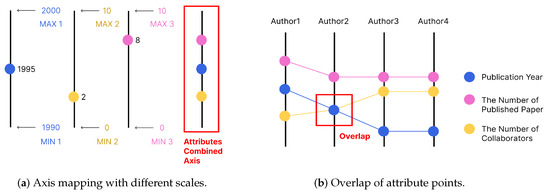
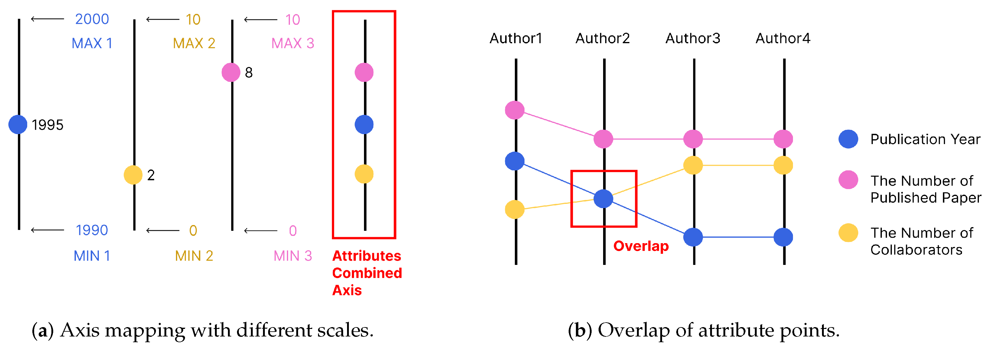
Finally, nodes are represented as axes, multivariate values of nodes are defined as points, and multiple attribute points are mapped on the same axis with length and color-code attribute categories. The attribute and node were combined based on the proximity principle. Axes are placed on the left and above ROI at corresponding nodes to maintain users’ original cognition of the traditional adjacency matrix and ensure the same starting point of nodes for easy comparison. In addition, each attribute’s value interval and distribution may differ significantly when multiple attributes are mapped on the axis simultaneously, and the problem of uneven distribution and severe occlusion will occur (G2). Therefore, we use a different scale approach: The maximum and minimum values of each attribute in the datasets are taken as their scale, and attributes of different scales are simultaneously mapped on the same axis (Figure 2a).
Figure 2.
Visual mapping of MVF.
3.3.2. Link
After axis and point visualization is completed, two problems are found: Points with different attributes may overlap completely on the axis (Figure 2b), and the location of covered points cannot be identified, resulting in information loss. A three-dimensional perspective environment will produce a parallax effect, and even attribute points have a common baseline, but the vanishing point of perspective angle causes length deformation, which is not convenient for attribute comparison between different nodes. To solve these problems, the link is added to the MVF.
The link connects the same attributes of adjacent nodes, and the slope of the link can be used to observe the changing trend of attribute values and identify outliers. Links with different slopes can identify completely overlapping points, alleviating the point overlap problem to some extent. The color mapping of the link is consistent with the attributes, which uses the similarity principle in Gestalt to connect the same attributes of different nodes with colors to form a whole to reduce users’ cognitive burden. All the above considerations aim to improve the efficiency of attribute recognition and comparison (G1).
3.4. Parallel Coordinate
An analysis of the tasks of the multivariate network shows that the detail display and comparison usually occur after target cluster identification. Therefore, the MVF is designed as a flexible auxiliary detail view of the ROI.
After the ROI selection is completed, the parallel coordinate will display all node attributes involved in the selected ROI, which is divided into two parts and placed perpendicular to the ROI plane (Figure 3c) to avoid the occlusion problem of all ROI edges and nodes and multivariate (G2).
Figure 3.
Details of MVF.
3.5. Interactions in Immersive Environment
The user can access and observe objects freely in the 6DOF immersion environment provided by virtual reality head-mounted display (VR HMD). The size and observation angle of the object can be directly adjusted with the movement of the body position and the rotation of the head. The basic interaction zoom and pan do not need to be completed indirectly through the traditional WIMP paradigm, thus speeding up exploration in the MVF.
4. Comparison with Embedded Model
4.1. Dataset
As an example dataset, we use a graph of DBLP to visualize the adjacency matrix. The dataset is provided in the supplementary Dataset S1 https://www.mdpi.com/article/10.3390/app122312182/s1. The graph consists of 12 articles, including 34 authors (the node of the graph). Three attributes (node multiple attributes) are taken for each author: the earliest publication year, the number of published papers, and the number of collaborators. The top notes are arranged in the same order from left to right, and the left nodes are from top to bottom.
The graph has 1156 edges. An edge represents the cooperation times of two authors, that is, how many articles they wrote together. The edge attributes are color-coded, and no other edge-related attributes are present in the dataset.
For our tasks, we assume the goal of an analyst is to locate author attributes and compare attributes through multiple nodes.
4.2. Scenarios for Comparison
- Scene 1:
- Adjacency Matrix with MVF
The MVF adjacency matrix focus view model is shown in Figure 4a. The parallel coordinate is divided into two segments arranged on the left and top of the ROI cluster. The axes that represent nodes are placed at the central point of the corresponding edges, and the attributes of each node are mapped on the axis. Links connect the same properties of adjacent nodes (see Figure 1b).
Figure 4.
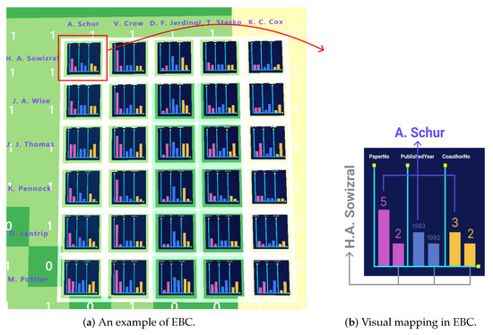
Details of the EBC model.
- Scene 2:
- Adjacency Matrix with Embedded Bar Chart (EBC)
To control variables, we migrate the traditional embedded view of the Embedded Bar Chart (EBC) to the same immersive environment as the MVF. The EBC model is shown in Figure 4a; attribute values are presented as a bar chart and placed on each edge. Each edge contains six attribute values belonging to two nodes, with three attribute values for each. The placing order of each group of attributes is consistent. That is, the value on the left of each group of attribute values belongs to the upper node, and the value on the right belongs to the left node. Attribute values are color-coded, consistent with the MVF (Figure 4b).
5. User Study
We conducted a controlled experiment to assess the performance of the MVF in terms of locating and comparing attributes of the ROI. The EBC was selected to be compared with the MVF. It is a between-subjects design, and the measures include task completion time, accuracy, and subjective satisfaction. The experiment program automatically recorded the task completion time and accuracy rate. After the experiment, users were required to fill in the questionnaire and participate in an interview.
5.1. Hypotheses
When the EBC is used, attributes often cause information redundancy, substantial limitation of attribute display space, and edge occlusion. All the above problems cause interference with the user’s judgment and lead to a long task completion time. On the basis of these considerations, we developed the following hypotheses, in the task of attribute localization and comparison:
- H1: The MVF accomplishes tasks faster than the traditional focus view model EBC.
- H2: MVF is more accurate than EBC when locating and comparing.
- H3: MVF can locate more easily than EBC.
- H4: MVF can perform comparisons more easily than EBC.
- H5: MVF is easier to understand than EBC.
- H6: Users prefer MVF to the EBC model.
5.2. Task
On the basis of the taxonomy of multidimensional visualization tasks by Eliane et al. (2006) [44], five tasks can be considered as goals: identity, determine, compare, infer, and locate. In Multivariate Network Visualization [45], tasks are divided into four categories: structure-based task, attribute-based task, browsing task, and estimation task. The attribute-based task contains node tasks and links tasks. We combine the two taxonomy methods above and focus our tasks on locating and comparing nodes’ attributes.
On the basis of Multivariate Network Visualization, the task is affected by the number of attributes involved. Hence, we designed four tasks, as shown below (Table 1). The first two tasks are for localizing, and the last two are for comparing. All four are independent tasks. The answer to the task may be one or more. The following is an example set of tasks:
Table 1.
Task taxonomy.
- T1: The name of the author with two publications in the cluster.
- T2: The name of the author with one cooperator and the publication year of 1993 in the cluster.
- T3: The name of the author with the fewest publications.
- T4: The name of the author with the earliest publication year and the largest number of publications.
The size of the selected cluster is also a variable that affects the experiment. The cluster in the experiment is divided into small, medium, and large sizes according to the total number of nodes (34 authors). Small size involves authors in the range of 1–11, medium size involves authors in the range of 12–22, and large size involves authors in the range of 23–34.
To ensure that every participant can complete the experiment, the answer for each task is set as the author’s name, which may be unique or multiple. If a wrong choice is made, then the correct rate is 0. If less is chosen, then the correct rate is calculated as the proportion of the number of correct answers.
We used the same selected cluster and tasks in the control group, with small, medium, and large clusters. Each cluster consists of four tasks. After all tasks in a cluster are complete, the next cluster will be replaced. The selected cluster and task order of T1–T4 were random. To control variables, the interaction (hovering and clicking) with gestures was consistent in both experiments. The two models were randomly assigned to different participants.
5.3. Apparatus
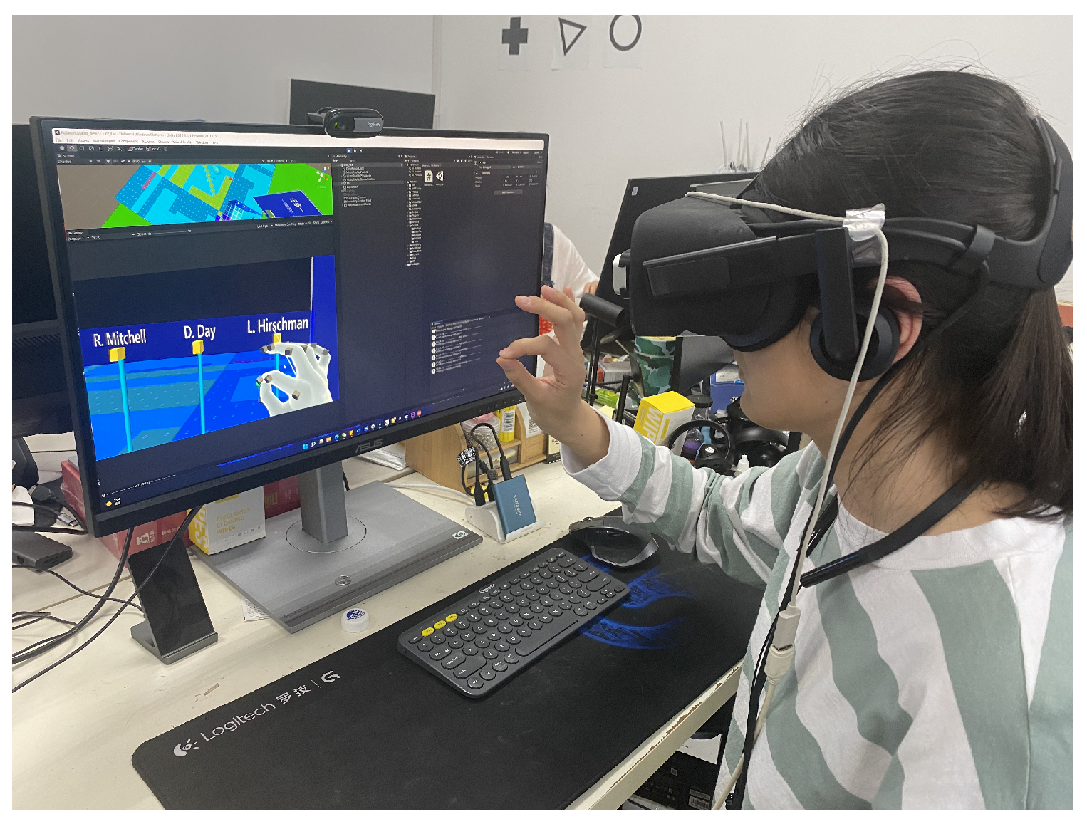
The hardware in the experiment is Oculus Rift VR HMD and Leap Motion. Oculus Rift is a VR device that provides a 3D virtual environment. Leap Motion is a hand-tracking device placed in front of Oculus Rift HMD for identifying hands in an immersive environment. It is only used for basic selection operations required in the task and will not substantially affect the experiment results. The experimental program is developed using the Unity platform and MRTK toolkit. The experiment was run on Windows 11 64-bit operation system, with an Intel (R) Core (TM) i5-9400F CPU 2.90 GHz, 32 GB RAM processor. The graphics card is NVIDIA GTX1060 (Figure 5).
Figure 5.
Hardware setup and experimental program interface.
5.4. Procedure
We recruited 20 graduate students on campus as participants, including 5 men and 15 women, who have normal color vision (no color blindness) and are right-handed. Fifteen of them knew the adjacency matrix in graph visualization, and six had experience in immersive analytics. We used a between-subjects design, and the participants were randomly assigned to two groups. Ten students participated in the experimental Scene1-MVF (two men, eight women), and the other 10 students participated in the experimental Scene2-EBC (three men, seven women). The participants wore a VR HMD display and sat on a chair with their hands about 15 cm in front of the Leap Motion (Figure 5).
The participants were first introduced to the basic knowledge of graph visualization, adjacency matrix mapping rules, multi-attribute mapping rules, and experimental tasks, then introduced to the essential operation in the virtual environment, and a group of pre-experiments were conducted the same VR experimental scenario. The pre-experiment was conducted in the order of small, medium, and large clusters to help the users gradually adapt to the difficulty. The formal experiment consisted of 9 clusters (three small, three medium, and three large). Only a pinch gesture was used in the whole experiment. The participants were advised to take a 5–10 min break in the middle of the experiment, and each participant spent about 60 min completing the experiment.
Each participant completed 4 tasks ∗ 9 clusters = 36 tasks in this scenario. Finally, we collected 20 participants ∗ 2 techniques ∗ 36 tasks = 1440 trials.
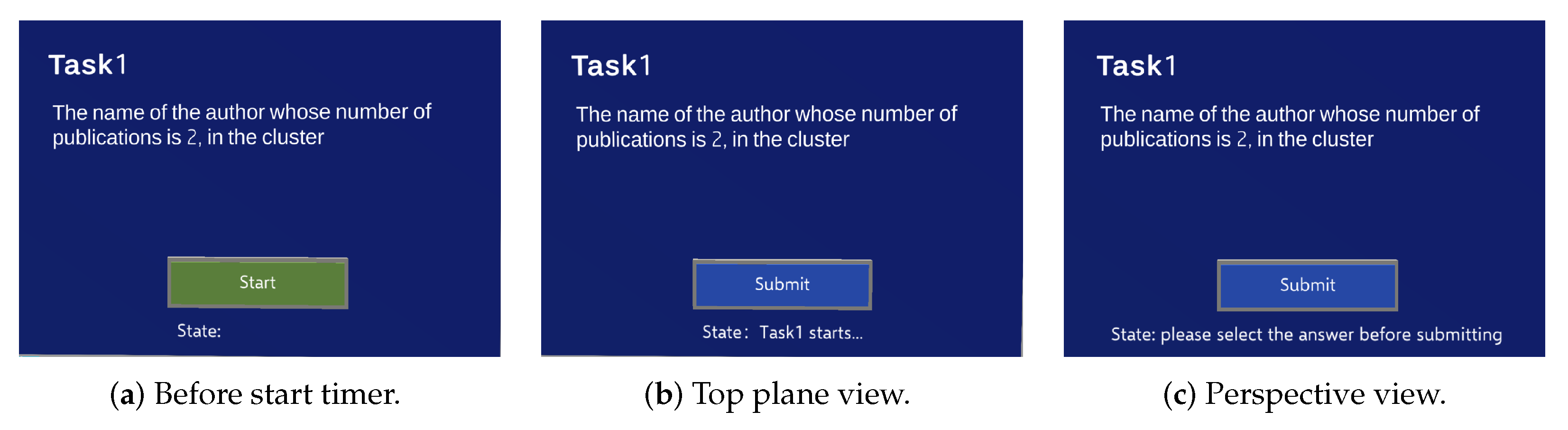
A task panel in VR includes the task number, task content, and a button that controls the start and end of the timer (Figure 6). After the user understands the task, they pinched “Start” button in the task panel to start timing, pinched the name tag of the node to select the task answer, and pinched the “Submit” button in the task panel to end timing and submit the answer after finishing the task. If the submitted answer is empty, then the submission cannot be made, and the timing will not end until one or more answers are successfully submitted. Once a trial is completed, the subsequent trial is displayed automatically until all four cluster trials have been conducted, and then, the next cluster with its tasks would appear.
Figure 6.
Task panel for timing in VR.
We asked the participants to complete tasks as quickly and accurately as possible, with each task completion time measured by the user pinching on the “Start” button and “Submit” buttons and accuracy as measured by the number of correct tasks in the group. After the user completes the task, the program automatically records and calculates the data. At the end of the experiment, the users were asked to experience the other model and then fill out Likert scales to reflect their subjective satisfaction. The questionnaire aims to evaluate the influence of two factors (position mapping and attribute occurrence quantity) on location, comparison, and comprehension. Q1–Q3 belong to the position factor, Q4–Q6 belong to the attribute occurrence quantity factor, and Q7 belongs to the preference of the two models. Except for Q7, each question has five choices: strongly disagree (1), disagree (2), not sure (3), agree (4), and strongly agree (5). These questions include the following:
- Q1: You think that the position mapping of the author and attributes is helpful for you to locate the attribute value.
- Q2: You think that the position mapping of the author and attributes is helpful for you to compare attribute values.
- Q3: You think that the position mapping of the author and attributes is helpful for you to understand the relationship between author and their attributes.
- Q4: You think that the attribute occurrence number is helpful for you to locate attribute values.
- Q5: You think that the attribute occurrence number is helpful for your to compare attribute values.
- Q6: You think that the attribute occurrence number is helpful for you to understand the relationship between the author and their attributes.
- Q7: Which model do you prefer?
5.5. Result
We used the paired t-test to analyze the collected completion time, accuracy, and questionnaire Likert scale data.
5.5.1. MVF Is Faster Than EBC
Table 2.
Means of completion time, with the standard deviation of the measured mean in seconds. Differences in accuracy are indicated by *. Significant differences in accuracy are indicated by **.
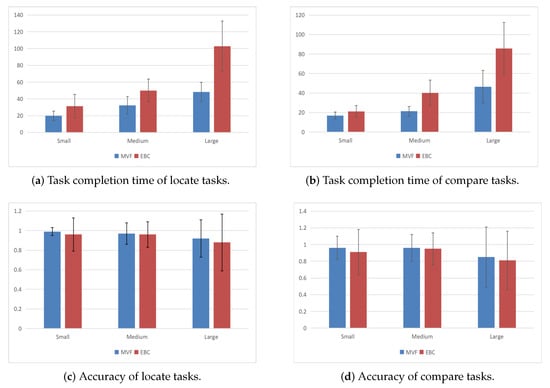
Figure 7.
Results regarding task completion time in seconds. Error bars indicate the standard deviation of the measured mean.
We found a significant effect of time for the model type. For both localization and comparison tasks, the MVF takes significantly less time than EBC. For the localization tasks, the completion time of the MVF is 63.6% (Table 2-➀ ➁), 64.6% (Table 3-➂ ➃), and 47% (Table 2-➄ ➅) of EBC in S (small), M (medium), and L (large) sizes, respectively. For L clusters, the advantage of the MVF is more obvious, and the completion time of the MVF is only 47% of that of EBC (Table 2-➄ ➅). For the comparison task, the completion time of the MVF was 80% (Table 2-➆ ➇), 52.8% (Table 2-➈ ➉), and 54.1% (Table 2-⑪ ⑫) of EBC on the scale of S, M, and L, respectively. For M and L clusters, the MVF has more obvious advantages, and its completion time accounts for only 52.8% (Table 2-➈ ➉) and 54.1% (Table 2-⑪ ⑫) of EBC (see Figure 7a).
Table 3.
Means of accuracy, with the standard deviation of the measured mean in percentages.
We also found a significant effect of size. As expected, completion time increased for the L cluster, especially the EBC. In terms of the localization tasks, for L clusters, the completion time of the EBC increased by 106% (Table 2- ➃ ➅), while the MVF increases by only 50% (Table 2-➂ ➄). In terms of comparison ability, for M clusters, the completion time of the EBC increased by 90.2% (Table 2-➇ ➉) while the MVF increased by only 25.6% (Table 2-➆ ➈) (Figure 7b). Hence, H1 was accepted.
5.5.2. No Significant Difference in Accuracy between MVF and EBC
The accuracy results are summarized in Table 3 and Figure 7c,d. No significant difference in accuracy was found between MVF and EBC for localization or comparison tasks. With the increase of the selected cluster size, the accuracy of localization and comparison tasks of both models decreased. Hence, H2 was rejected.
5.5.3. MVF Can Locate More Easily Than EBC
Table 4.
Means of Likert scale questionnaire, with the standard deviation of the measured mean in seconds. Differences in accuracy are indicated by *. Significant differences in accuracy are indicated by **.
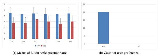
Figure 8.
Results of task completion time in seconds. Error bars indicate the standard deviation of the measured mean.
From Q1, “You find it easier to locate the attribute if it appears only/more than once” and Q4, “You find the position mapping of the attributes is easier for you to locate the attribute”, we found that the MVF and the EBC have a significant difference in how easily they can locate. Users generally think the MVF can locate more easily. The scores of the MVF were significantly higher than those of the EBC for both attribute occurrence times (Table 4-➀ ➂) and position mapping (Table 4-➂ ➃) factors. Hence, H3 was accepted.
5.5.4. MVF Can Perform Comparisons More Easily Than EBC
From Q2, “You find it’s easier to compare attribute values between authors if the attribute appears only/more than once” and Q5, “You find the position mapping of the attributes is easier for you to compare attribute values between authors”, we found that the MVF and EBC have significant differences in comparability. The MVF can perform comparisons more easily for common tasks. The score of the MVF was significantly higher than that of EBC in both attribute occurrence times (Table 4-➄ ➅) and position mapping (Table 4-➆ ➇) factors. In addition, the MVF was larger than the EBC (Table 4-➆ ➇) with an average difference of 1.3 points in position mapping, indicating that the attribute location of the MVF was conducive to attribute comparison. At the same time, EBC was relatively unfavorable to the comparison. Hence, H4 was accepted.
5.5.5. MVF Is Easier to Understand Than EBC
From Q3, “You find it’s easier to understand the relationship between the author and attributes if the attribute appears only/more than once” and Q6, “You find the position mapping of the attributes is easier for you to understand the relationship between the author and attributes”, we found that the MVF and the EBC have significant differences in incomprehensibility. The MVF is easier to understand for common tasks. The scores of the MVF were significantly higher than those of the EBC for both quantitative factors (Table 4-➈ ➉) and location factors (Table 4-⑪ ⑫). Moreover, the difference between the quantitative factors MVF and EBC was larger (Table 4-⑪ ⑫), with an average difference of 1.7 points, indicating that the occurrence times of the MVF attributes were helpful to the understanding of the model. At the same time, the EBC was relatively unfavorable to the understanding. Hence, H5 was accepted.
5.5.6. Users Prefer MVF to EBC Model
The results are summarized in Figure 8b.
From Q7, “Compare the MVF and the EBC and choose the model you prefer”, we found that users prefer the MVF to the EBC model. All users prefer the MVF model, while no users prefer the EBC model. This finding indicates that the MVF model is significantly better than the EBC model in completing the localization and comparison tasks. Hence, H6 was accepted.
6. Discussion
6.1. Efficiency
During the localization, the MVF was less affected by community size because all attributes of the MVF had a unified baseline. A specific attribute could be used as the basis for screening and positioning, significantly improving localization efficiency. However, no unified baseline was available the EBC column elements, making comparison difficult. Moreover, the MVF can see more attributes in the diagonal corner, and the head rotation amplitude is smaller when browsing all attributes, thus saving more time. During the comparison, the EBC was more affected by community size because when too many column nodes were present (M, L clusters), the attributes that were not on the same baseline increased. Moreover, because the column was too long, head rotation was needed to assist observation, so it took more time. Unlike localization, which requires only a single browse, the comparison may require repeated observations between distant areas, which is why the time assumption increased dramatically in M and L clusters. However, in the MVF, users could find a suitable angle to view more attributes in the immersive environment, and the head rotation amplitude and times were less than the EBC, thus taking less time. Some users said in the interview that the redundant information of EBC is too much and dense, which disturbs their judgment. Observing large clusters even requires large body movements, which makes it impossible to derive an overview of the data, increasing the burden of memory and making it more time consuming. The above findings show that the MVF has higher efficiency than the EBC when localizing and comparing, suggesting that the MVF has no redundant data and makes the interface simpler. The MVF provides a unified baseline for all attributes, which is more intuitive. The VR immersion environment can give an overview angle in the MVF, decreasing the need to remember the data from the visual field. Moreover, users can observe details without tremendous body and head movements.
6.2. Accuracy
No significant difference in accuracy was found between the MVF and the EBC, and the accuracy decreased with the increase in cluster size. We suggest that the MVF could increase efficiency while maintaining accuracy. When the cluster size increases, more nodes and attributes are involved, which is why the error probability is higher.
6.3. Localization Ability
The MVF can locate more accessible than the EBC. Regarding the number of attribute occurrences, EBC’s fastest and most accurate localization method (observing one row and one column) still causes redundant information about one author’s attribute. At the same time, no duplicate data exist in the MVF model. Hence, the MVF is more concise and clear. Regarding position mapping, the order of two juxtaposed attributes in the EBC needs to be memorized repeatedly, which causes a cognitive burden. The MVF has a unified baseline, which is why it convenient for users to quickly filter and locate through height based on a specific value. However, this locating method may cause some errors due to the perspective effect in an immersive environment. Some users mentioned in the interview that the attributes on the left will be unconsciously regarded as the attributes of the author on the left, but this is not the mapping rule in EBC. However, the left column contains the attributes of the author on the top, making it difficult to remember. Moreover, the attributes in the middle are far away from the author’s name, whch is why they may deviate from the row or column when locating. The MVF, on the other hand, does not need to remember the relationship between the author and their attribute because they are placed closer.
6.4. Comparison Ability
The MVF can compare more accessible than the EBC. Regarding the number of attribute occurrences, EBC may repeatedly compare attributes because the corresponding author of the juxtaposition attribute can easily remember incorrectly. Regarding position mapping, all attributes of MVF are on the same horizontal plane, and attribute values can be intuitively compared through the broken line trend. In addition, the upper and left parallel coordinates form an angle, significantly reducing the user’s browsing range.
6.5. Comprehensive Ability
The MVF is easier to understand than the EBC. Regarding the number of attribute occurrences, most users overthought information in the EBC, bringing negative emotions and causing loss of interest, whereas the MVF is more intuitive and straightforward. Regarding position mapping, according to the Gestalt proximity principle, users take the information close as a group. In the EBC, the column on the lower right is far away from the author’s name, thus causing serious confusion to users. However, the MVF uses axes to connect the author’s name with attributes, which fits the property and is easier to understand.
6.6. User Preference
In quantity, users dislike redundant information, which interferes with their judgment. In terms of position, users want to group elements directly through location placement to minimize memory burden. In terms of physical exertion, users prefer not to move too much. Therefore, the MVF is more consistent with user preferences than the EBC.
6.7. VR Immersive Environment Influence
The VR immersive environments have both advantages and disadvantages for data analysis. The advantage is that VR supports natural observation, and slight zoom, and angle rotation are easy to achieve. Finding the perfect viewing angle is easy in a VR environment. The disadvantage is that significant scale movement may cause fatigue. Moreover, VR can cause vertigo due to the low frame rate. Moreover, VR is not suitable for long-time wear. Continuous use of VR for more than 1 h causes apparent visual fatigue.
7. Conclusions
We propose a focus view model of an adjacency matrix named MVF, using parallel coordinates and the third spatial dimension to provide node attributes. Through this approach, all ROI information will not be blocked, and the relationship between nodes and attributes will be clear. No redundant multivariate information is present in the MVF, and the position mapping conforms to users’ cognition of the traditional adjacency matrix, allowing users to quickly locate and compare node attributes. We conducted a user study to evaluate the performance of the MVF. The results show that the MVF is more efficient and accurate than the EBC in locating and comparing attributes. The position mapping and single attribute occurrence in the MVF are easier to understand than in the EBC. Users have a strong preference for the MVF. In future work, we will improve the perspective of space and apply our model to the focus view in other multivariate graphs.
Supplementary Materials
The following supporting information can be downloaded at: https://www.mdpi.com/article/10.3390/app122312182/s1, Dataset S1: Datasets and Details for MVF Evaluation.
Author Contributions
Conceptualization, T.L.; Software, Y.J. and S.L.; Validation, S.W.; Resources, S.W.; Writing—original draft, T.L. and Y.J.; Writing—review & editing, T.L.; Visualization, Y.J.; Project administration, T.L.; Funding acquisition, T.L. All authors have read and agreed to the published version of the manuscript.
Funding
This work was supported by the National Natural Science Foundation of China (61702042).
Institutional Review Board Statement
Not applicable.
Informed Consent Statement
Written informed consent has been obtained from the participant(s) to publish this paper.
Data Availability Statement
Not applicable.
Conflicts of Interest
The authors declare no conflict of interest. The funders had no role in the design of the study; in the collection, analyses, or interpretation of data; in the writing of the manuscript, or in the decision to publish the results.
Abbreviations
The following abbreviations are used in this manuscript:
| VR | Virtual Reality |
| IA | Immersive Analytics |
| ROI | Region of Interest |
| F+C | Focus + Context |
| HMD | Virtual Reality Head-Mounted Display |
| MVF | Multivariate Fence |
| EBC | Embedded Bar Chart |
| PCP | Parallel Coordinate Plot |
| PM | Position Mapping |
| NoO | Number of Occurrence |
References
- Chen, Y.; Guan, Z.; Zhang, R.; Du, X.; Wang, Y. A survey on visualization approaches for exploring association relationships in graph data. J. Vis. 2019, 22, 625–639. [Google Scholar] [CrossRef] [Scilit]
- Dinkla, K.; Westenberg, M.A.; Van Wijk, J.J. Compressed Adjacency Matrices: Untangling Gene Regulatory Networks. IEEE Trans. Vis. Comput. Graph. 2012, 18, 2457–2466. [Google Scholar] [CrossRef] [Scilit] [PubMed]
- Kister, U.; Klamka, K.; Tominski, C.; Dachselt, R. G ra S p: Combining Spatially-aware Mobile Devices and a Display Wall for Graph Visualization and Interaction. Comput. Graph. Forum 2017, 36, 503–514. [Google Scholar] [CrossRef] [Scilit]
- Burch, M.; Brinke, K.B.T.; Castella, A.; Peters, G.K.S.; Shteriyanov, V.; Vlasvinkel, R. Dynamic graph exploration by interactively linked node-link diagrams and matrix visualizations. Vis. Comput. Ind. Biomed. Art 2021, 4, 23. [Google Scholar] [CrossRef] [Scilit] [PubMed]
- Elmqvist, N.; Do, T.-N.; Goodell, H.; Henry, N.; Fekete, J.-D. ZAME: Interactive Large-Scale Graph Visualization. In Proceedings of the 2008 IEEE Pacific Visualization Symposium, Kyoto, Japan, 5–7 March 2008; pp. 215–222. [Google Scholar] [CrossRef] [Scilit]
- Horak, T.; Berger, P.; Schumann, H.; Dachselt, R.; Tominski, C. Responsive Matrix Cells: A Focus+Context Approach for Exploring and Editing Multivariate Graphs. IEEE Trans. Vis. Comput. Graph. 2020, 27, 1644–1654. [Google Scholar] [CrossRef] [Scilit] [PubMed]
- Henry, N.; Fekete, J.-D. MatrixExplorer: A Dual-Representation System to Explore Social Networks. IEEE Trans. Vis. Comput. Graph. 2006, 12, 677–684. [Google Scholar] [CrossRef] [Scilit]
- Dwyer, T.; Marriott, K.; Isenberg, T.; Klein, K.; Riche, N.; Schreiber, F.; Stuerzlinger, W.; Thomas, B.H. Immersive Analytics: An Introduction. In Immersive Analytics. Lecture Notes in Computer Science; Springer: Cham, Switzerland, 2018; Volume 11190. [Google Scholar] [CrossRef]
- Fonnet, A.; Prié, Y. Survey of Immersive Analytics. IEEE Trans. Vis. Comput. Graph. 2021, 27, 2101–2122. [Google Scholar] [CrossRef] [Scilit]
- Chandler, T.; Cordeil, M.; Czauderna, T.; Dwyer, T.; Glowacki, J.; Goncu, C.; Klapperstueck, M.; Klein, K.; Marriott, K.; Schreiber, F.; et al. Immersive Analytics. In Proceedings of the 2015 Big Data Visual Analytics (BDVA), Hobart, Australia, 22–25 September 2015; pp. 1–8. [Google Scholar] [CrossRef] [Scilit]
- Yang, Y.; Dwyer, T.; Marriott, K.; Jenny, B.; Goodwin, S. Tilt Map: Interactive Transitions between Choropleth Map, Prism Map and Bar Chart in Immersive Environments. IEEE Trans. Vis. Comput. Graph. 2020, 27, 4507–4519. [Google Scholar] [CrossRef] [Scilit] [PubMed]
- Yang, Y.; Xia, W.; Lekschas, F.; Nobre, C.; Krüger, R.; Pfister, H. The Pattern is in the Details: An Evaluation of Interaction Techniques for Locating, Searching, and Contextualizing Details in Multivariate Matrix Visualizations. In Proceedings of the 2022 CHI Conference on Human Factors in Computing Systems (CHI’22), New Orleans, LA, USA, 29 April–5 May 2022; Article 84. Association for Computing Machinery: New York, NY, USA, 2022; pp. 1–15. [Google Scholar] [CrossRef] [Scilit]
- Spindler, M.; Stellmach, S.; Dachselt, R. PaperLens: Advanced magic lens interaction above the tabletop. In Proceedings of the ACM International Conference on Interactive Tabletops and Surfaces (ITS’09), Banff, AB, Canada, 23–25 November 2009; Association for Computing Machinery: New York, NY, USA, 2009; pp. 69–76. [Google Scholar] [CrossRef] [Scilit]
- Kister, U.; Reipschläger, P.; Matulic, F.; Dachselt, R. BodyLenses: Embodied Magic Lenses and Personal Territories for Wall Displays. In Proceedings of the 2015 International Conference on Interactive Tabletops & Surfaces (ITS’15), Madeira, Portugal, 15–18 November 2015; Association for Computing Machinery: New York, NY, USA, 2015; pp. 117–126. [Google Scholar] [CrossRef] [Scilit]
- Dostal, J.; Hinrichs, U.; Kristensson, P.O.; Quigley, A. SpiderEyes: Designing attention- and proximity-aware collaborative interfaces for wall-sized displays. In Proceedings of the 19th International Conference on Intelligent User Interfaces (IUI’14), Haifa, Israel, 24–27 February 2014; Association for Computing Machinery: New York, NY, USA, 2014; pp. 143–152. [Google Scholar] [CrossRef] [Scilit]
- Elhart, I.; Scacchi, F.; Niforatos, E.; Langheinrich, M. ShadowTouch: A Multi-user Application Selection Interface for Interactive Public Displays. In Proceedings of the 4th International Symposium on Pervasive Displays (PerDis’15), Saarbruecken, Germany, 10–12 June 2015; Association for Computing Machinery: New York, NY, USA, 2015; pp. 209–216. [Google Scholar] [CrossRef] [Scilit]
- Elmqvist, N.; Henry, N.; He, Y.R.; Fekete, J.-D. Melange: Space folding for multi-focus interaction. In Proceedings of the SIGCHI Conference on Human Factors in Computing Systems (CHI’08), Florence, Italy, 5–10 April 2008; Association for Computing Machinery: New York, NY, USA, 2015; pp. 1333–1342. [Google Scholar] [CrossRef] [Scilit]
- Butscher, S.; Hornbæk, K.; Reiterer, H. SpaceFold and PhysicLenses: Simultaneous multifocus navigation on touch surfaces. In Proceedings of the 2014 International Working Conference on Advanced Visual Interfaces (AVI’14), Como, Italy, 27–29 May 2014; Association for Computing Machinery: New York, NY, USA, 2014; pp. 209–216. [Google Scholar] [CrossRef] [Scilit]
- Butscher, S. Explicit & Implicit Interaction Design for Multi-Focus Visualizations. In Proceedings of the Ninth ACM International Conference on Interactive Tabletops and Surfaces (ITS’14), Dresden, Germany, 16–19 November 2014; Association for Computing Machinery: New York, NY, USA, 2014; pp. 455–460. [Google Scholar] [CrossRef] [Scilit]
- Chiu, P.; Liao, C.; Chen, F. Multi-touch document folding: Gesture models, fold directions and symmetries. In Proceedings of the SIGCHI Conference on Human Factors in Computing Systems (CHI’11), Vancouver, BC, Canada, 7–12 May 2011; Association for Computing Machinery: New York, NY, USA, 2011; pp. 1591–1600. [Google Scholar] [CrossRef] [Scilit]
- Langner, R.; Satkowski, M.; Büschel, W.; Dachselt, R. MARVIS: Combining Mobile Devices and Augmented Reality for Visual Data Analysis. In Proceedings of the 2021 CHI Conference on Human Factors in Computing Systems (CHI’21), Yokohama, Japan, 8–13 May 2021; Article 468. Association for Computing Machinery: New York, NY, USA, 2021; pp. 1–17. [Google Scholar] [CrossRef] [Scilit]
- Bach, B.; Pietriga, E.; Fekete, J.-D. Visualizing dynamic networks with matrix cubes. In Proceedings of the SIGCHI Conference on Human Factors in Computing Systems (CHI’14), Toronto, ON, Canada, 26 April–1 May 2014; Association for Computing Machinery: New York, NY, USA, 2014; pp. 877–886. [Google Scholar] [CrossRef] [Scilit]
- Alper, B.; Bach, B.; Riche, N.H.; Isenberg, T.; Fekete, J.-D. Weighted graph comparison techniques for brain connectivity analysis. In Proceedings of the SIGCHI Conference on Human Factors in Computing Systems (CHI’13), Paris, France, 27 April–2 May 2013; Association for Computing Machinery: New York, NY, USA, 2013; pp. 483–492. [Google Scholar] [CrossRef] [Scilit]
- Yi, J.S.; Elmqvist, N.; Lee, S. TimeMatrix: Analyzing Temporal Social Networks Using Interactive Matrix-Based Visualizations. Int. J. Human-Computer Interact. 2010, 26, 1031–1051. [Google Scholar] [CrossRef] [Scilit]
- Nobre, C.; Meyer, M.; Streit, M.; Lex, A. The State of the Art in Visualizing Multivariate Networks. Comput. Graph. Forum 2019, 38, 807–832. [Google Scholar] [CrossRef] [Scilit]
- Abello, J.; van Ham, F. Matrix Zoom: A Visual Interface to Semi-External Graphs. In Proceedings of the IEEE Symposium on Information Visualization, Austin, TX, USA, 10–12 October 2004; pp. 183–190. [Google Scholar] [CrossRef] [Scilit]
- Viau, C.; McGuffin, M.J.; Chiricota, Y.; Jurisica, I. The FlowVizMenu and Parallel Scatterplot Matrix: Hybrid Multidimensional Visualizations for Network Exploration. IEEE Trans. Vis. Comput. Graph. 2010, 16, 1100–1108. [Google Scholar] [CrossRef] [Scilit]
- Ko, S.; Afzal, S.; Walton, S.; Yang, Y.; Chae, J.; Malik, A.; Jang, Y.; Chen, M.; Ebert, D. Analyzing high-dimensional multivaríate network links with integrated anomaly detection, highlighting and exploration. In Proceedings of the 2014 IEEE Conference on Visual Analytics Science and Technology (VAST), Paris, France, 25–31 October 2014; pp. 83–92. [Google Scholar] [CrossRef] [Scilit]
- Bezerianos, A.; Chevalier, F.; Dragičević, P.; Elmqvist, N.; Fekete, J. GraphDice: A System for Exploring Multivariate Social Networks. Comput. Graph. Forum 2010, 29, 863–872. [Google Scholar] [CrossRef] [Scilit]
- Bach, B.; Dachselt, R.; Carpendale, S.; Dwyer, T.; Collins, C.; Lee, B. Immersive Analytics: Exploring Future Interaction and Visualization Technologies for Data Analytics. In Proceedings of the 2016 ACM International Conference on Interactive Surfaces and Spaces (ISS’16), Niagara Falls, ON, Canada, 6–9 November 2016; Association for Computing Machinery: New York, NY, USA, 2016; pp. 529–533. [Google Scholar] [CrossRef] [Scilit]
- Cordeil, M.; Cunningham, A.; Dwyer, T.; Thomas, B.H.; Marriott, K. ImAxes: Immersive Axes as Embodied Affordances for Interactive Multivariate Data Visualisation. In Proceedings of the 30th Annual ACM Symposium on User Interface Software and Technology (UIST’17), Quebec City, QC, Canada, 22–25 October 2017; Association for Computing Machinery: New York, NY, USA, 2017; pp. 71–83. [Google Scholar] [CrossRef] [Scilit]
- Sicat, R.; Li, J.; Choi, J.; Cordeil, M.; Jeong, W.-K.; Bach, B.; Pfister, H. DXR: A Toolkit for Building Immersive Data Visualizations. IEEE Trans. Vis. Comput. Graph. 2018, 25, 715–725. [Google Scholar] [CrossRef] [Scilit] [PubMed]
- Cordeil, M.; Cunningham, A.; Bach, B.; Hurter, C.; Thomas, B.H.; Marriott, K.; Dwyer, T. IATK: An Immersive Analytics Toolkit. In Proceedings of the 2019 IEEE Conference on Virtual Reality and 3D User Interfaces (VR), Osaka, Japan, 23–27 March 2019; pp. 200–209. [Google Scholar] [CrossRef] [Scilit]
- Liu, J.; Prouzeau, A.; Ens, B.; Dwyer, T. Design and Evaluation of Interactive Small Multiples Data Visualisation in Immersive Spaces. In Proceedings of the 2020 IEEE Conference on Virtual Reality and 3D User Interfaces (VR), Atlanta, GA, USA, 22–26 March 2020; pp. 588–597. [Google Scholar] [CrossRef] [Scilit]
- Hayatpur, D.; Xia, H.; Wigdor, D. DataHop: Spatial Data Exploration in Virtual Reality. In Proceedings of the 33rd Annual ACM Symposium on User Interface Software and Technology (UIST’20), Virtual Event, 20–23 October 2020; Association for Computing Machinery: New York, NY, USA, 2020; pp. 818–828. [Google Scholar] [CrossRef] [Scilit]
- Satriadi, K.A.; Ens, B.; Cordeil, M.; Czauderna, T.; Jenny, B. Maps Around Me. Proc. ACM Hum.-Comput. Interact. 2020, 4, 201. [Google Scholar] [CrossRef] [Scilit]
- Zhao, Y.; Shi, J.; Liu, J.; Zhao, J.; Zhou, F.; Zhang, W.; Chen, K.; Zhao, X.; Zhu, C.; Chen, W. Evaluating Effects of Background Stories on Graph Perception. IEEE Trans. Vis. Comput. Graph. 2021, 28, 4839–4854. [Google Scholar] [CrossRef] [Scilit]
- Whitlock, M.; Smart, S.; Szafir, D.A. Graphical Perception for Immersive Analytics. In Proceedings of the 2020 IEEE Conference on Virtual Reality and 3D User Interfaces (VR), Atlanta, GA, USA, 22–26 March 2020; pp. 616–625. [Google Scholar] [CrossRef] [Scilit]
- Inselberg, A.; Dimsdale, B. Parallel coordinates: A tool for visualizing multi-dimensional geometry. In Proceedings of the First IEEE Conference on Visualization: Visualization’90, San Francisco, CA, USA, 23–26 October 1990; pp. 361–378. [Google Scholar] [CrossRef] [Scilit]
- Kobayashi, H.; Furukawa, T.; Misue, K. Parallel Box: Visually Comparable Representation for Multivariate Data Analysis. In Proceedings of the 2014 18th International Conference on Information Visualisation, Paris, France, 16–18 July 2014; pp. 183–188. [Google Scholar] [CrossRef] [Scilit]
- Johansson, J.; Cooper, M.; Jern, M. 3-dimensional display for clustered multi-relational parallel coordinates. In Proceedings of the Ninth International Conference on Information Visualisation (IV’05), London, UK, 6–8 July 2005; pp. 188–193. [Google Scholar] [CrossRef] [Scilit]
- Artero, A.O.; de Oliveira, M.C.F.; Levkowitz, H. Uncovering clusters in crowded parallel coordinates visualizations. In Proceedings of the IEEE Symposium on Information Visualization, Austin, TX, USA, 10–12 October 2004; pp. 81–88. [Google Scholar]
- Bok, J.; Kim, B.; Seo, J. Augmenting Parallel Coordinates Plots With Color-Coded Stacked Histograms. IEEE Trans. Vis. Comput. Graph. 2020, 28, 2563–2576. [Google Scholar] [CrossRef] [Scilit] [PubMed]
- Valiati, E.R.A.; Pimenta, M.S.; Freitas, C.M.D.S. A taxonomy of tasks for guiding the evaluation of multidimensional visualizations. In Proceedings of the 2006 AVI Workshop on BEyond Time and Errors: Novel Evaluation Methods for Information Visualization (BELIV’06), Venice Italy, 23 May 2006; Association for Computing Machinery: New York, NY, USA, 2006; pp. 1–6. [Google Scholar] [CrossRef] [Scilit]
- Archambault, D.; Abello, J.; Borner, K.; Diehl, S.; Dwyer, T.; Elmqvist, N.; Fekete, J.D.; Gou, L.; Hagen, H.; Holten, D.; et al. Multivariate Network Visualization. In Proceedings of the Dagstuhl Seminar 13201, Dagstuhl Castle, Germany, 12–17 May 2013; Springer: Cham, Switzerland, 2013; Volume 8380. [Google Scholar]

Publisher’s Note: MDPI stays neutral with regard to jurisdictional claims in published maps and institutional affiliations. |
© 2022 by the authors. Licensee MDPI, Basel, Switzerland. This article is an open access article distributed under the terms and conditions of the Creative Commons Attribution (CC BY) license (https://creativecommons.org/licenses/by/4.0/).