


Abstract
Methane emissions from plugged and unplugged abandoned wells dilute rapidly with air, causing conventional detection methods to fall short of detecting methane leaks from these sources. Commonly used technologies for methane emission detection often fall short of the detection limit required for low-rate emissions from abandoned wells, and are either dependent on environmental conditions or costly and highly energy consuming, barring them from becoming a scalable solution to this problem. We introduce here a new system for outdoor testing and show how the flux chamber detection limit is progressively reduced from 700 g/h to 2 g/h and ultimately to 1 g/h, meeting the US Department of the Interior (DOI) standard for monitoring equipment used on abandoned wells. Field deployment on an actual abandoned well also revealed intermittent emissions, which may serve as an indicator of deteriorating well integrity over time when monitored periodically. To forecast the emission event timing and intensity, a Liquid Time-Constant (LTC) and a gated recurrent neural network were trained on methane concentration time series collected during field deployment. As available well sites for physical testing are limited and atmospheric conditions are not controllable, a computational fluid dynamics (CFD) simulation framework integrated with machine learning (ML) was developed to optimize wellhead chamber geometry and size for both detectability and safety. This chamber is designed to be used for testing well sites in mass number that helps well abandonment ranking systems for both operators and regulatory bodies.
1. Introduction
According to the 2024 Orphaned Wells Program Annual Report to Congress [1], 141,959 wells have been reported as orphaned by the Interstate Oil and Gas Compact Commission. As orphaned wells do not have a solvent operator, their responsibility is transferred to the federal government or states, which can affect their monitoring due to lack of funding. This lack of testing makes a low-cost, scalable testing method urgently necessary. An orphaned well, by its technical definition, is a well that does not have an assigned operator, which is distinct from a plugged and abandoned well, where the well has been sealed using cement and flow barriers. This study targets abandoned wells, defined as wells that have been left in either a plugged or unplugged state, regardless of their ownership. Estimated numbers of potential sources are reported by several studies: Townsend-Small et al. (2016) [2] estimate at least 2.3 million abandoned wells in the onshore United States, the California Council on Science and Technology [3] reports 2.5 million non-productive wells, and Kang et al. (2014) [4] cite an estimated 3 million abandoned wells nationwide. The differences among these estimates are due to incomplete historical records and wells that were drilled before the advent of regulatory documentation requirements.
Commonly used methods in methane emission detection and measurement vary in detection limit and coverage area. This variance can fundamentally change the usefulness of each case. Methane detection satellites such as TROPOMI cover a larger land area but have high detection limits. Dubey et al. [5] reported a detection limit of 500–8800 kg/h/pixel in a single overpass, which is more suitable for landfills and coal mines and is unsuitable for abandoned wells with low emission rates [6]. Aerial technologies, including LiDAR-based airborne methods, detect emissions in the 100–1000 kg/h range at high altitude, with sensitivity improving to approximately 0.5 kg/h in close proximity to the source [6]. Ground surveys carried out by high-flow samplers and static flux chambers are useful for detecting emissions at 1 g/h or lower [6].
Qi et al. (2021) [7] examined the time required for gas to migrate to the top of a low-permeability cement column. Simulations covered different API gravity oils and vertical permeabilities. Results demonstrated that vertical permeability in the cement works as a path for gas emission to the top of the well.
The US Department of the Interior Methane Measurement Guidelines [6] classify wells into four types based on measurement feasibility. A Type 1 well, by definition, is a well that can be easily covered by a portable chamber. This research focuses only on Type 1 wells, which lack wellhead assemblies or production lines. The guidelines set the minimum detection limit for measurement equipment used on abandoned wells at 1 g/h. Previous ground-based studies report wide-ranging emission rates from abandoned wells. Townsend-Small et al. (2016) [2] measured a national average leak rate of 1.38 g/h across 138 plugged and unplugged wells using flux chambers and high-flow samplers, with only 1 of the plugged wells and 8 of 20 unplugged wells showing detectable emissions. Kang et al. (2014) [4] reported an average of 0.27 kg/d using a static flux chamber, though this value was strongly influenced by a small number of super-emitting wells, as the mean leak rate of all tested wells exceeded the median by three orders of magnitude. Riddick et al. (2020) [8] observed that emissions at individual wells varied over 24 h periods with rates ranging from 0.2 to 81,000 mg of CH4/h. The average of the recorded emission rates varied by a factor of 18, with variability ranging from factors of 1.1 to 142 across different wells.
Haase et al. (2025) [9] demonstrated that burying the edges of a rigid flux chamber to a depth of at least 18 cm, combined with wetting the surrounding soil to reduce pore volume and improve compaction, significantly reduced gas leakage around the chamber base and improved measurement reliability. Consistent with these findings, the edges of our chamber were similarly buried in wet soil to minimize lateral gas escape and ensure a tight seal around the well.
Currently, no existing method provides continuous, low-cost monitoring of Type 1 wells at detection limits consistent with DOI standards. This study fills this gap through three contributions. First, it presents the iterative process of the physical design of a smart static flux chamber, progressing through controlled outdoor experiments and optimized by analyzing the data collected during the experiments to achieve a detection limit of 1 g/h, which was later validated on an abandoned well. Second, it demonstrates the use of a recurrent neural network, such as a Liquid Time-Constant neural network, to forecast leak event timing and intensity using live data collected in the field, enabling the chamber to function without the need for long-term or permanent installation. Third, it provides a computational fluid dynamics framework combined with machine learning-based optimization of chamber geometry for both detectability and safety. Results of simulation and optimization are used to design a chamber tailored to each well’s dimensions. The prototype tested in this study is inexpensive and can be redeployed on multiple wells, reducing per-well monitoring costs, which can be further lowered through mass production.
2. Materials and Methods
The methodology follows four phases: (1) sensor development through controlled indoor and outdoor testing for iterative chamber design, (2) field deployment on an abandoned well, (3) time-series forecasting using neural networks on field recorded data, and (4) computational fluid dynamics simulation coupled with machine learning optimization. Throughout this paper, the terms ’static flux chamber’ and ’canopy’ are used interchangeably; ’static flux chamber’ is the standard terminology used in the methane monitoring literature, while ’canopy’ refers to the specific ventilated structure developed in this study.
2.1. Sensor Development and Smart Integration
The methane sensor used in this study is a Molecular Property Spectrometer (MPS)-type sensor with a micromachined silicon transducer that measures the molecular properties of air to identify its composition. The sensor model is MPS003 (NevadaNano) with a lower detection limit of 50 parts per million (ppm) according to the specification provided by the manufacturer. This sensor is programmed to sample at a 3 s rate.
The MPS methane sensor is calibration-free according to the manufacturer specification. The sensor is certified with a 50 ppm detection limit which is validated by the manufacturer across the full −40 to 75 °C temperature range and 0 to 100% relative humidity, with built-in compensation for temperature, pressure, and humidity. The sensor holds Class 1, Division 1 intrinsic safety, which are relevant for deployment near leaking wells where flammable atmospheres may be present. It is important to mention that efforts mentioned in this paper have been around the safety-first mindset of the team. The sensor used in this project has a real-time monitoring capability and simulations have accounted for the most extreme scenarios that we have not witnessed in the field test. Experiments both conducted controlled and field conditions have shown concentration levels recorded are not rising to the lower explosive limit (LEL) of methane as the chamber is open to the atmosphere. The sensor was tested once in the laboratory using a pure methane high-pressure flux chamber and required no further field calibration during the duration of this study, consistent with the manufacturer specification operational lifetime without recalibration. Information regarding the sensor specification is available at manufacturer sensor documents [10,11].
A wind sensor manufactured by Calypso Instruments (Ultra-Low-Power Ultrasonic Wind Meter PRO, ULP PRO) was used to measure wind speed. This sensor was always deployed within 2 m of the methane sensor at 85 cm height from the ground to reduce near-ground wind speed noise and to approximate the height of the chamber opening. The sensor covers a wind speed range of 0.5–45 m/s.
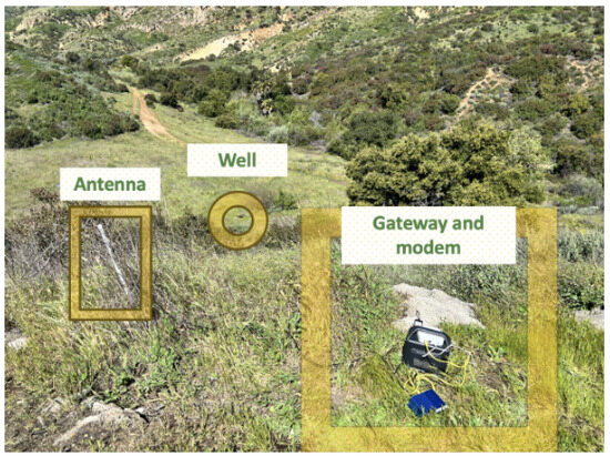
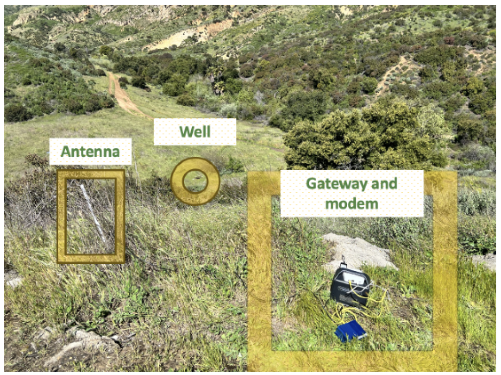
Both sensors were integrated into a communication system that transmits data to a USC-owned cloud storage platform via a cellular network or local gateway. Figure 1 shows the antenna connected to the local gateway, as cellular coverage was not available at the field test location. When cellular coverage is available, the sensor connects to the cloud via a SIM card and operates on a power bank with solar power generation capabilities. When cellular coverage is unavailable, a local antenna and lithium battery pack are required. The sensor system is estimated to last approximately 2 months without solar power generation, which far exceeds the 4–7 h data collection sessions conducted in this study.
Figure 1.
Field deployment of the IoT communication system. The local antenna (left) is positioned near the edge of the valley for optimal connectivity to the flux chamber deployed at the well location (center). A mobile power unit (right) connects the modem and gateway to the antenna.
2.2. Controlled Outdoor Testing: Iterative Design Optimization
Because the chamber performance must be evaluated under varying wind speeds and gusts, the testing was conducted outdoors. A high-pressure methane canister with 99.9% purity (GASCO) was connected to high-precision rotameters (FM-1050 Series, MATHESON, ±5% full-scale accuracy) to simulate a leaking well and optimize chamber geometry before field deployment on an abandoned well. Different chamber configurations were tested to determine how detection performance varies with design parameters.
2.2.1. First Design: Suspended Sensors
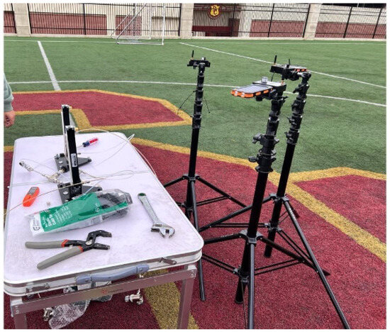
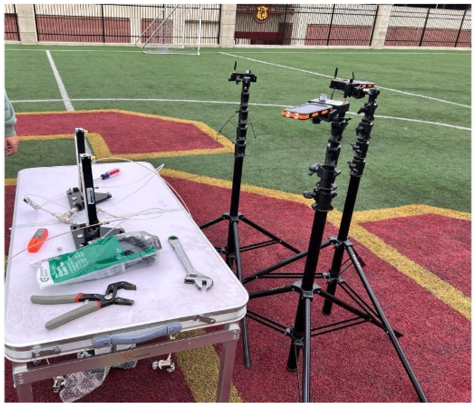
The first attempt at methane detection was through sensors that were hung on tripods at different heights around leak sources to establish the baseline of the methane detection capability of our sensor without an isolating chamber. Figure 2 shows the three sensors on tripods positioned 25–35 cm from the leaking rotameters at 150 cm above ground level. Based on this configuration, partial isolation of the emission source by a chamber was determined to be necessary to reduce the rate of methane–air mixing.
Figure 2.
Baseline detection configuration with sensors mounted on tripods at 15–25 cm horizontal distance from the leak sources and 150 cm above ground level. Two rotameters (left) are placed on a table, one can leak at 0.5–70 g/h and the other at 50–1200 g/h.
2.2.2. Second Design: Aluminum Ventilation Chamber
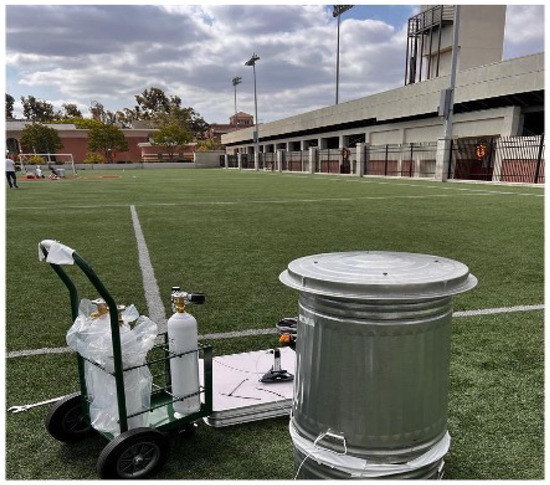
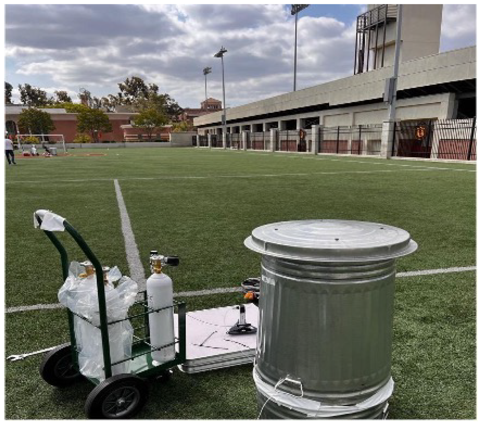
The next major variation tested was a 32-gallon aluminum cylindrical chamber with a circular lid (21 inches in diameter) placed on top of the chamber. The top of the chamber has a punched hole covered by the lid (different punched hole radii were tested, covering 10–75% of the lid radius), with a 1–5 cm height difference between the top of the chamber and the lid; this configuration is shown in Figure 3.
Figure 3.
The aluminum chamber with its lid (right). The chamber top has a punched hole, and the lid has a slight height difference, allowing air inside and methane outside of the chamber. The methane canister connected to rotameters (left) simulates a continuously leaking well. Wind speed during this test has been conducted in calm conditions where wind speed does not rise higher than 2 m/s.
2.2.3. Third Design: Wind-Shielded Configuration
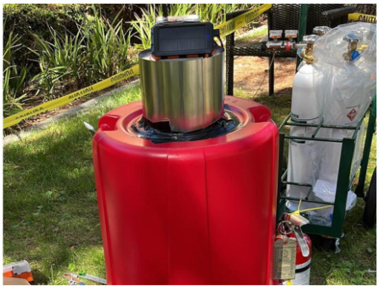
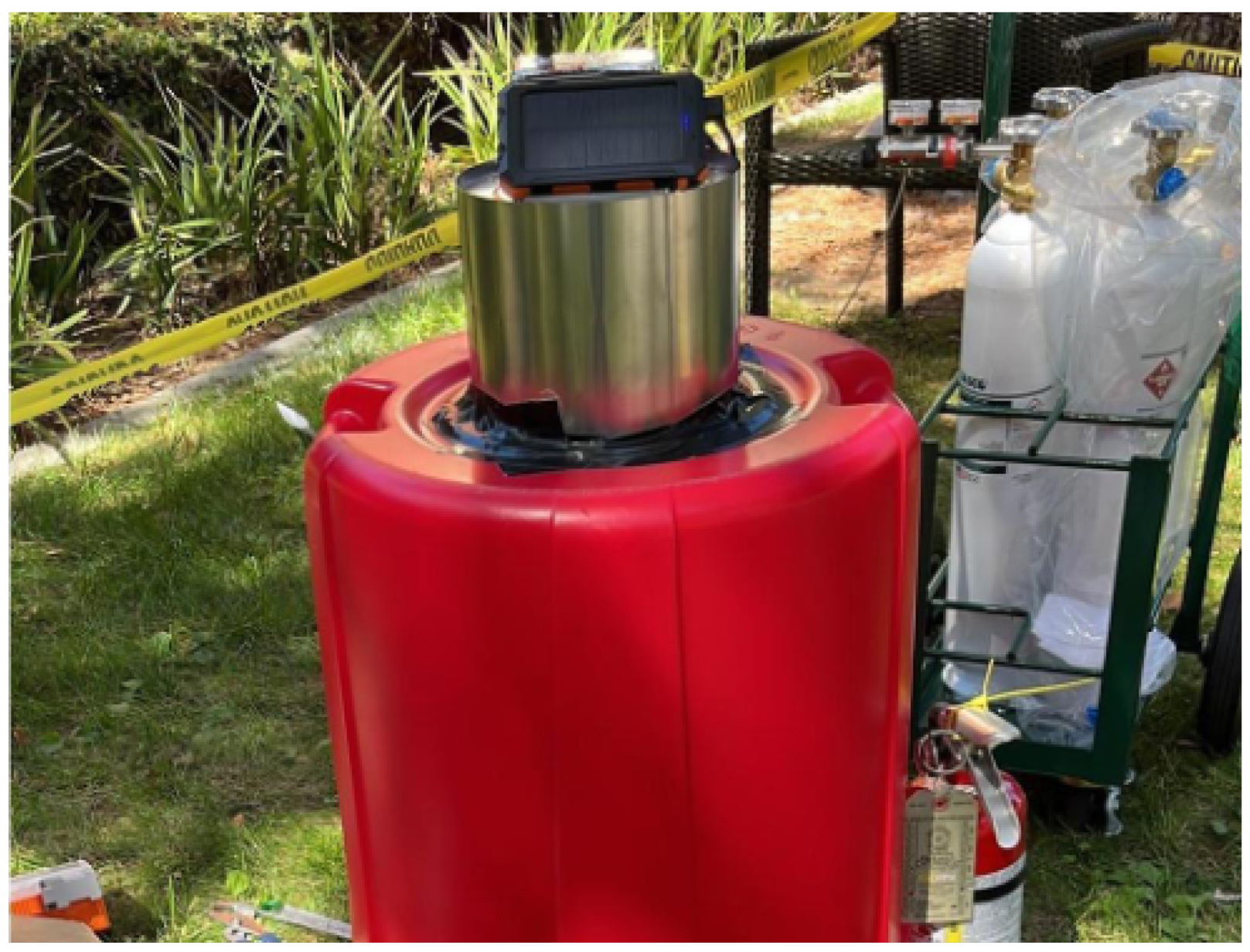
To address signal fluctuation observed in the second design and to accommodate the possibility of intermittent emissions at real well sites, a steel sheet was wrapped around the wind cap to further limit methane–air mixing. The wind cap is a Dura-Vent model with a 10.5-inch outer diameter, wrapped in a steel sheet with a 1 mm air gap between the vent and the wrapping. The methane sensor was suspended within the wind cap at 15 inches from the top of the wind cap, which is approximately 3 inches lower than the punched hole opening. The communication kit and battery pack were mounted atop the wind cap, as shown in Figure 4. Different chamber configurations were tested at 10 distinct methane leak rate steps over 40 h of outdoor controlled testing, with a minimum duration of 20 min per testing step. Chamber geometry and methane leak rate were controlled variables in these experiments, while wind speed varied naturally with ambient atmospheric conditions.
Figure 4.
The third chamber design, constructed from plastic for improved portability with a steel-wrapped wind cap on top. The wind cap provides ventilation so that the space under the chamber is not isolated from the atmosphere. The methane sensor is housed inside the wind cap (not visible), while the communication kit and battery pack are mounted on top. This test has been conducted in calm conditions where wind speed does not rise higher than 3 m/s.
2.3. Field Deployment on Abandoned Well
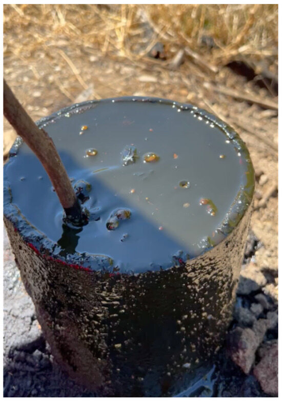
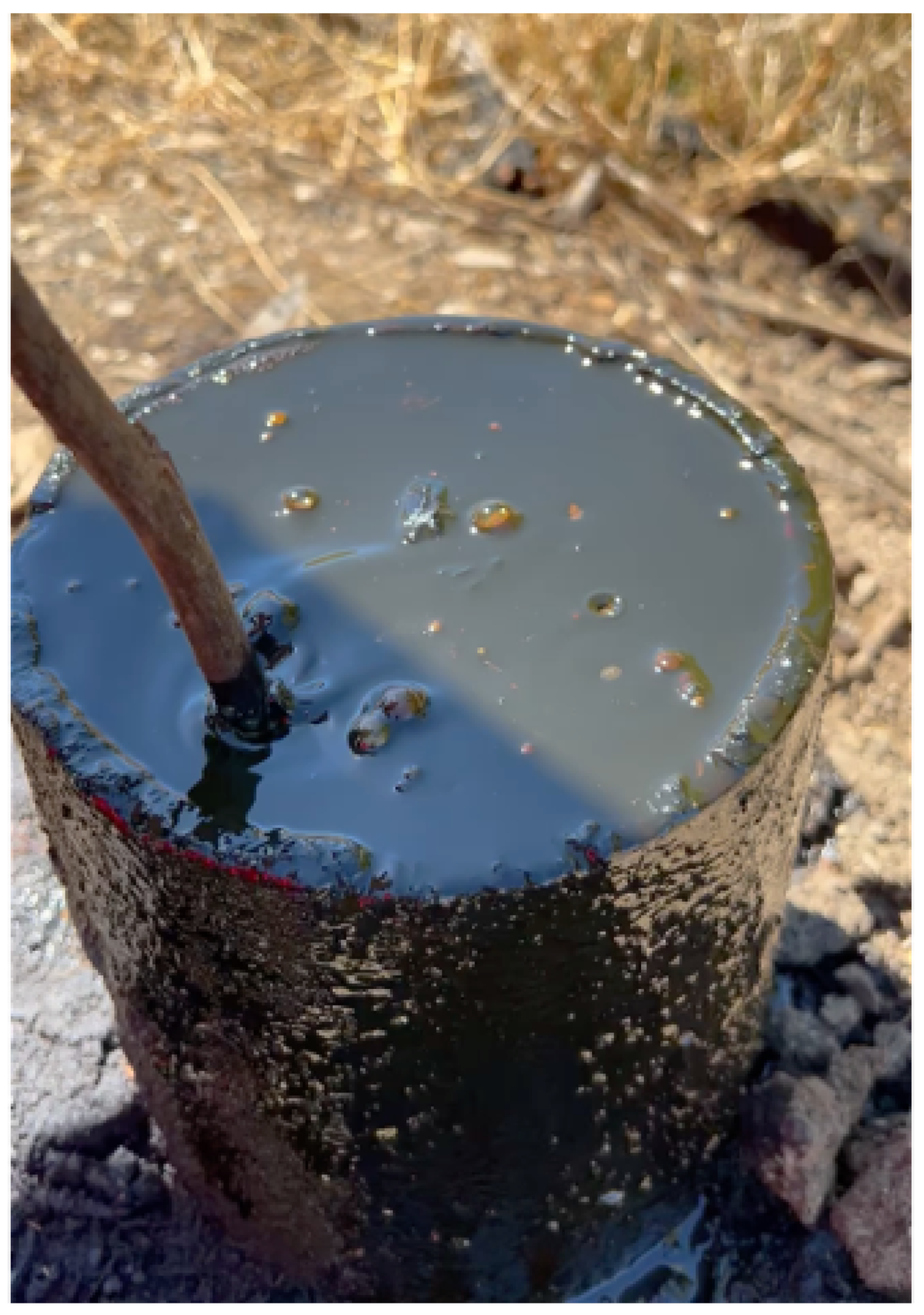
Site selection criteria included a publicly accessible location and a visible surface with dimensions matching the Type 1 category of the DOI guidelines. The tested well is located in the north of Los Angeles county and was abandoned in 1951 using partial cementing and a wooden plug, according to CalGEM WellFinder records. The well exhibited gas bubbling and fresh crude seepage at the time of testing. As the chamber could not be left at the well site overnight, the well was tested during multiple sessions lasting 4–7 h within a 6-month period. The lower detection limit of the methane sensor (50 ppm), combined with the sensor being positioned inside the chamber, reduces the risk of interference from methane plumes originating from nearby sources other than the well itself. Figure 5 shows the condition of this well, including oil seepage and gas bubbling.
Figure 5.
The abandoned well used for field testing, showing crude oil seepage and gas bubbling at the surface. The site is located in the Los Angeles area on a publicly accessible hiking path.
2.4. Time-Series Forecasting with Neural Networks
Permanent chamber installation increases theft risk and potential methane accumulation in addition to having a large physical footprint. As permanent installation or long-term testing is not possible, time-series forecasting models were developed to predict methane leak events from limited field data to capture the statistical profile of each well that enables assessment of well integrity degradation with time through periodic monitoring.
Two recurrent neural network architectures were evaluated: Gated Recurrent Unit (GRU) and Liquid Time-Constant (LTC) networks [12,13]. Both models were trained during a deployment session (6279 samples, 7 h and 11 min) using an 80–20 train–test split. Data were normalized to the 0–1 range prior to training. The deployment sensor recorded methane concentration, temperature, pressure, and relative humidity at a programmed interval of 3 s. Initial training attempts incorporated all environmental features alongside methane concentration, which showed no performance improvement; therefore, in the final model, the methane concentration time series was used as the sole input.
The goal of using AI in this study is not to predict instantaneous leak values from a single deployment, but rather to capture the statistical profile of leak events at a given well from a few hours of testing that the chamber can practically perform. After consulting with stakeholders, leaving the flux chamber on the well site overnight was determined to be impractical due to theft risk and the large footprint of the chamber in the open environment. Periodic deployments, in which the chamber is brought back to the same well site after several months (for example, three months, six months, or one year later), yield new test data that can be modeled using the predictions of the model trained on the prior deployment data. The difference between predicted and newly recorded leak frequency and intensity can indicate how the condition of the well has deteriorated during the elapsed period. The underlying assumption here is that the formation pressure and gas available near the well have not changed, which is reasonable for plugged and abandoned wells as they do not leak substantial methane volume. To prevent the model from memorizing the data, the time series was split chronologically rather than randomly, with the first 80% used for training and the final 20% held out for testing. This split guarantees that the test set consists entirely of future observations that the model has never seen during training. The model is trained to predict the next single sample, which forces it to learn the temporal dependence structure rather than memorize specific leak concentration values. The 15 to 25% undershooting in the prediction of peak concentrations reported in Section 3.3 is consistent with a model that has learned the average temporal pattern of the data rather than memorized individual extreme events.
To improve model performance, hyperparameter optimization was performed using the Optuna framework with 30 trials per model configuration. Table 1 summarizes parameters that were optimized using the hyperparameter optimizer over the range specified and Table 2 presents specific information regarding the final architecture of the models used.
Table 1.
Hyperparameter search configuration (applied to all models).
Table 2.
Optimized model’s configuration.
2.5. COMSOL-MATLAB-ML Optimization Framework
As most wells are unavailable for testing in Southern California, and atmospheric conditions such as wind speed are not controllable, optimizing chamber geometry to enhance detection capability while minimizing unsafe methane concentration buildup was conducted through computational fluid dynamics sweep simulations across all design parameters.
2.5.1. Computational Model (COMSOL Multiphysics 6.4)
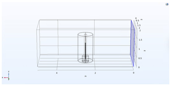
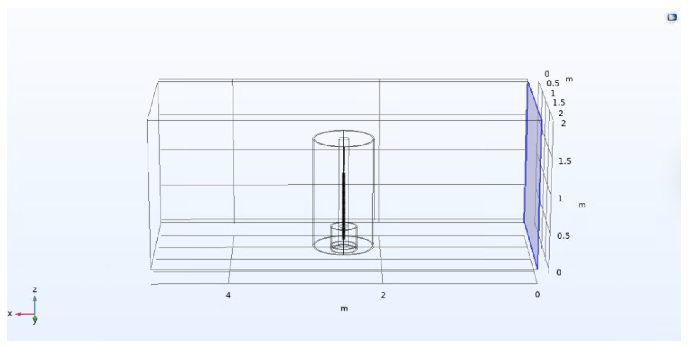
A cylindrical chamber was modeled in the center of a rectangular domain (5 m × 2 m × 2 m) in the COMSOL Multiphysics 6.4 geometry environment; a well was placed inside the chamber cylinder, and a hole was placed on top of the chamber cylinder. Wind enters from one side of the domain under an inflow velocity boundary condition. Initial methane concentration was set to zero throughout the domain at . The bottom of the chamber and the domain was assigned a closed (no-slip) boundary condition, while all other surfaces (except the inlet) were set to zero gauge pressure. The computational domain, including the well and chamber geometry, is shown in Figure 6. Species transport was modeled using a methane–air binary diffusion coefficient of 0.221 cm2/s at standard temperature (298 K) and atmospheric pressure (101.325 kPa) with gravity enabled, as reported in NIST Technical Note 2279; Burgess, 2024 [14]. The simulations in this study employ a laminar flow model, which accounts for both convective transport by the velocity field and molecular diffusion. In practice, wind in when it comes in contact with structures is expected to produce turbulent flow, where additional mixing occurs due to velocity fluctuations and eddies that are absent in laminar flow. Karim et al. (1987) [15] showed experimentally that methane disperses into air significantly faster under turbulent conditions. The diffusion coefficient in turbulent airflow is three to four orders of magnitude larger than molecular diffusion due to these turbulent eddies. As the laminar model does not capture this additional turbulent mixing, it will overestimate local methane concentrations compared to what would occur under turbulent conditions. As a result, the danger zones identified in this study represent conservative estimates, and the recommended flux chamber designs carry a built-in safety margin when applied to actual field conditions where turbulent mixing is present.
Figure 6.
Computational domain used in COMSOL Multiphysics simulations. The dark blue surface indicates the wind inlet boundary with an inflow velocity condition. The domain bottom is assigned a closed boundary, and all remaining surfaces are set to zero gauge pressure.
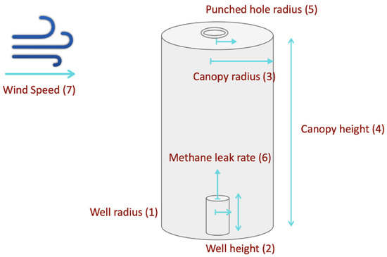
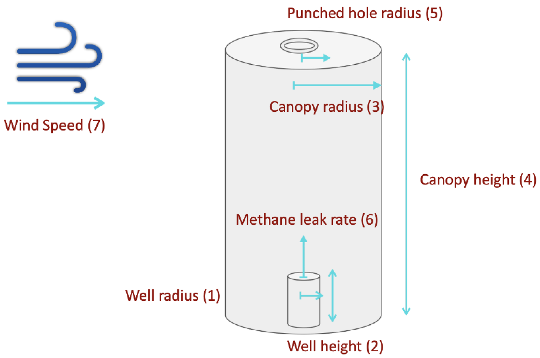
The seven governing design parameters are shown in Figure 7. Simulating methane dispersion under the chamber requires modeling both convection and diffusion, which is achieved using the Laminar Flow (spf) and Transport of Concentrated Species (tcs) modules in COMSOL Multiphysics 6.4.
Figure 7.
The seven governing design parameters for chamber optimization. Well height (W_height) and well radius (W_r) are the only parameters known to the operator; wind speed (A_q) and methane leak rate (M_q) are not under operator control. The remaining three parameters (C_height, C_r, PH_r) are determined through optimization. The arrows in this figure are either pointing at the direction of the fluid flow or helping to locate the parameter used in design.
The laminar flow module solves the incompressible Navier–Stokes equations for the velocity field. The momentum and continuity equations are given by Equation (1) (Incompressible Equation (2) Navier–Stokes COMSOL, 2024)):
where is the fluid density (kg/m3), is the velocity vector (m/s), t is time (s), p is the pressure (Pa), is the identity matrix, is the viscous stress tensor defined for a Newtonian incompressible fluid as with being the dynamic viscosity (Pa×s), is the volume force vector (N/m3), and is the gravitational acceleration vector (m/s2). Gravity is enabled in the simulation with a reference pressure of 1 atm and a reference temperature of 293.15 K.
The Transport of Concentrated Species module solves a mass balance equation governing the diffusion of methane into air. The nonconservative form of the species transport equation, as implemented in (COMSOL 2024), is given by Equation (3):
where is the mass fraction of species i (dimensionless), is the diffusive mass flux vector of species i (kg/(m2 × s)), and is the reaction rate for species i (kg/(m3 × s)). In this study, no chemical reactions occur between methane and air; therefore .
2.5.2. Two-Phase Parametric Study
Three objectives were formulated based on the fraction of the 1000 observation points falling within each methane concentration zone at min. The primary objective of this part of our research is to maximize the fraction of space inside of the chamber to fall within the detection window (50–50,000 ppm). This window is based on the sensor’s detection limit and lower explosive limit of methane (50,000 ppm), which ensures leaked methane is detected safely. Another optimization constraint in this task is minimizing the fraction of space inside the chamber that is above the lower explosive limit (LEL ≥ 50,000 ppm). Minimizing space above this threshold prevents unsafe methane accumulation inside the chamber. The last objective of this optimization is to minimize the volumetric fraction below the detection limit (<50 ppm), which reduces the probability of missed detection events.
The safety constraint is treated as a hard constraint and takes more weight over the two other objectives. Among feasible designs satisfying the safety constraint, the primary detection objective governs the optimization, with the secondary objective used to distinguish between designs of equivalent primary performance. Table 3 demonstrates each parameter baseline and range.The baseline is only used in phase 1 (35 simulations) of the simulation attempt where one parameter is swept and others are kept at the baseline. Phase 2 (193 simulations) of the simulations uses the Latin hypercube sampling technique to randomly choose one specific set of parameters for each simulation. Two geometric feasibility constraints were enforced during sampling: flux chamber height must exceed well height by at least 1 cm (C_height > W_height + 0.01 m), and flux chamber radius must exceed well radius by at least 1 cm (C_r > W_r + 0.01 m). The opening radius was sampled as a fraction of the flux chamber radius (PH_r = [0.10 to 0.90] × C_r) to maintain geometric proportionality.
Table 3.
Parameter baselines and ranges used in the two-phase parametric study. Baseline values are used in Phase 1, where one parameter is swept while all others are held constant. Phase 2 uses Latin hypercube sampling to simultaneously vary all parameters across the full range. All simulations are time-dependent and range from 0 to 1 min in 0.1 min steps.
2.5.3. Machine Learning Design Optimization Model
One recurrent neural network (GRU) was trained to predict the fraction of observation points falling within each concentration level (over LEL, detection window, and below detection limit) within the chamber as a function of the seven design parameters and time rather than predicting raw concentration values. The outputs of this model are indicators of optimization performance in fulfilling the objectives.
The network takes an eight-dimensional input at each of the 11 timesteps, corresponding to the seven design parameters (A_q, C_height, W_height, C_r, W_r, PH_r, M_q) and time. The input is processed by two stacked GRU layers with 128 and 64 hidden units respectively, each followed by batch normalization and dropout (rates of 0.3 and 0.2). The GRU output is then passed through two time-distributed dense layers of 32 and 16 neurons with ReLU activation and dropout (rates of 0.2 and 0.1), followed by a three-neuron Softmax output layer that ensures the three predicted zone fractions sum to 100% at each timestep. The network was compiled with the Adam optimizer (initial learning rate = 0.0005, loss function = categorical cross-entropy) and trained for up to 500 epochs with a batch size of 16. Early stopping (patience = 40 epochs) and learning rate reduction on plateau (factor = 0.5, patience = 15 epochs, minimum learning rate = ) were applied to prevent overfitting and ensure convergence. The simulation dataset was partitioned into training (80%), validation (10%), and test (10%) sets using random splitting with a fixed seed for reproducibility.
2.5.4. Design Recommendation Software
A design recommendation tool was developed based on the trained model that is computationally cheaper, faster, and easier to use for field operators without requiring knowledge of computational fluid dynamics or machine learning. The tool accepts two inputs, which are well radius (W_r) and well height (W_height). These two parameters are the only parameters known by the operators prior to the deployment. The results of this optimization are the chamber radius, chamber height, and punched hole radius for the given well. Optimization was performed using differential evolution, a global optimization algorithm well-suited to multi-parameter design spaces, applied over the full feasible parameter ranges defined in Table 3.
One recommended design is a conservative configuration, which prioritizes the safety objective, while the second design recommendation is a detection-optimized configuration that prioritizes the maximization of space under the chamber that falls in the detection window. The optimization software uses two inputs, which are well radius and well height, and the output of the software is the rest of the design parameters, such as chamber radius, chamber height, and punched hole radius, which are optimized by objective functions. The choice of weighting coefficients (1000 vs. 0.5 vs. 1 for the conservative design and 50 vs. 10 vs. 1 for the detection-optimized design) reflects the hierarchy in which safety, detection, and missed-detection penalties are ranked by the operator. A sensitivity analysis exploring the robustness of the recommended chamber geometries to variations in these weights is provided in the Supplementary Materials.
Conservative design objective function:
Detection-optimized design objective function:
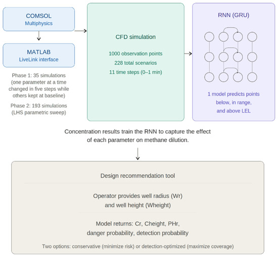
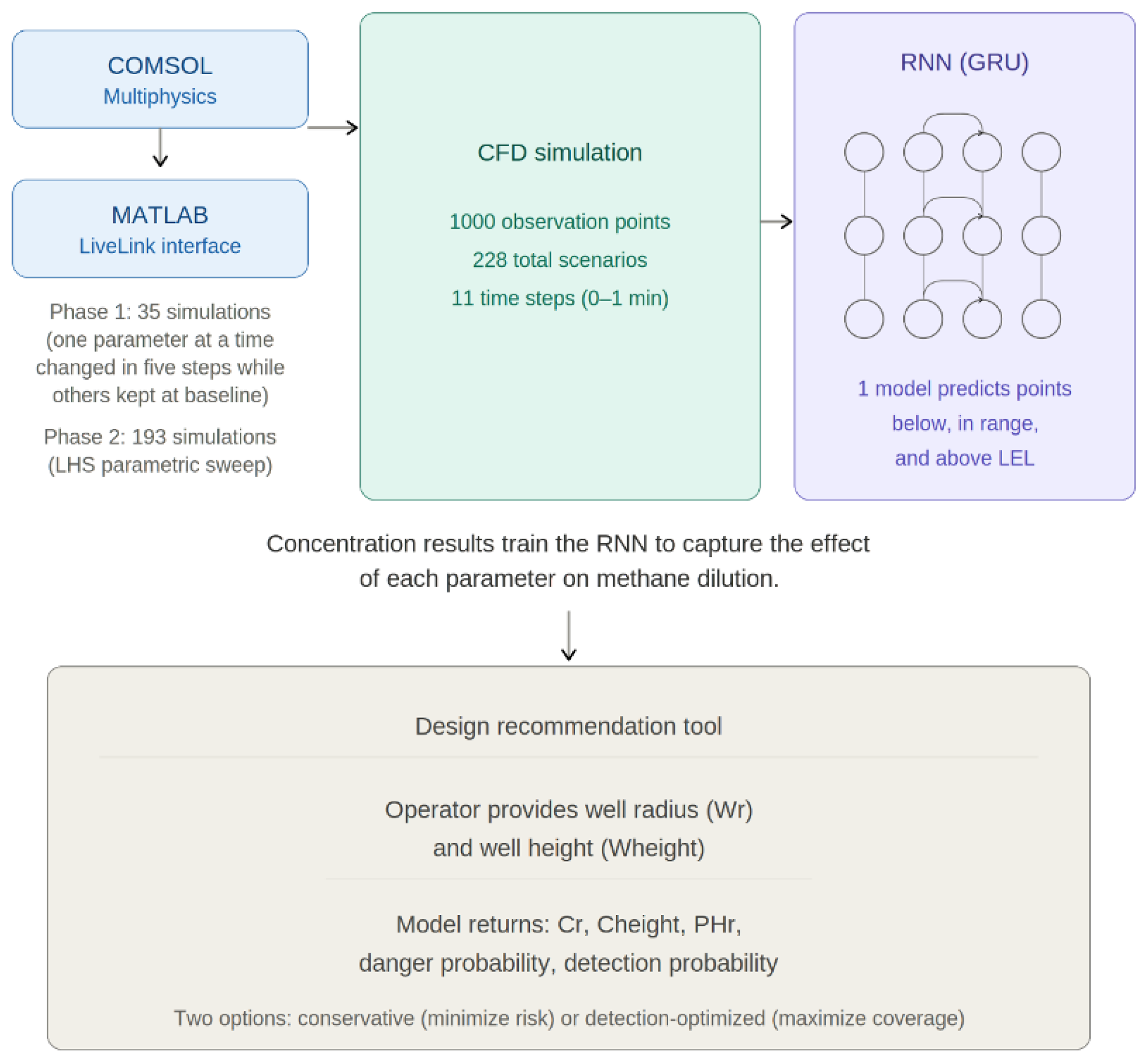
where , , and are the predicted number of observation points (out of 1000) in the above-LEL, detection-window, and below-detection zones, respectively. The conservative design applies a 1000-fold penalty to unsafe zone points and only a 0.5-fold reward to detection, prioritizing elimination of explosive risk. The detection-optimized design reduces the LEL penalty to 50-fold while increasing the detection reward to 10-fold, allowing the optimizer to accept marginally higher LEL risk in exchange for substantially improved detection coverage. In both formulations, below-detection points carry a unit penalty. The workflow of this optimization is demonstrated in Figure 8, which is a combination of COMSOL Multiphysics and its MATLAB LiveLinks interface and recurrent neural networks.
Figure 8.
The integrated COMSOL–MATLAB–ML optimization workflow. Parameter combinations are generated via Latin hypercube sampling and evaluated through automated COMSOL 6.4 simulations using MATLAB Livelink, producing 1000 spatially distributed methane concentration observations per run. The resulting dataset trains one recurrent neural network to predict concentration zone distributions. The trained surrogate model is subsequently used by the design optimization software to recommend chamber configurations within minutes.
Although the total number of simulations (228) may appear modest, each simulation records methane concentration at 1000 spatially randomly distributed observation points across 11 timesteps. The dataset was partitioned into training (80%), validation (10%), and test (10%). It is important to note that the task of the surrogate model is not to predict the exact concentration in parts per million at every observation point, which would be a substantially harder prediction problem. Instead, the model predicts the fraction of the 1000 observation points falling within each of three concentration zones (below detection, detection window, and above LEL) at each timestep. This aggregate metric is what governs the optimization objectives defined in Equations (4) and (5), so the accuracy required from the surrogate is the accuracy of the zone-fraction prediction rather than the accuracy of the point-wise concentration prediction. Model codes are available in the depository (link to this depository can be found in the data availability section).
3. Results
3.1. Controlled Outdoor Testing
The DOI has published guidelines that set methane detection from plugged and unplugged wells at 1 g/h; this standard shaped our goal for designing our static flux chamber. The progression of design iterations produced a decrease in detection limit from 700 g/h to 1 g/h. The first design, consisting of sensors mounted on poles, achieved detection only at 700 g/h of continuous methane leak and only when wind speed was below 1 m/s and blowing toward the sensors. The second design incorporated an aluminum chamber, which reduced the detection limit to 2 g/h. This design was highly unstable, showing washout and fluctuations. The third design achieved the target detection limit of 1 g/h with improved signal stability, making it suitable for testing on an abandoned well.
The 1 g/h detection limit reported in this study is defined by the methane leak rate controlled by the high-precision rotameters used to simulate the well leak. The rotameters were operated at a set point of 1 g/h, which corresponds to the established leak rate that the chamber successfully detected during the outdoor testing sessions.
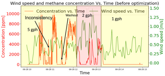
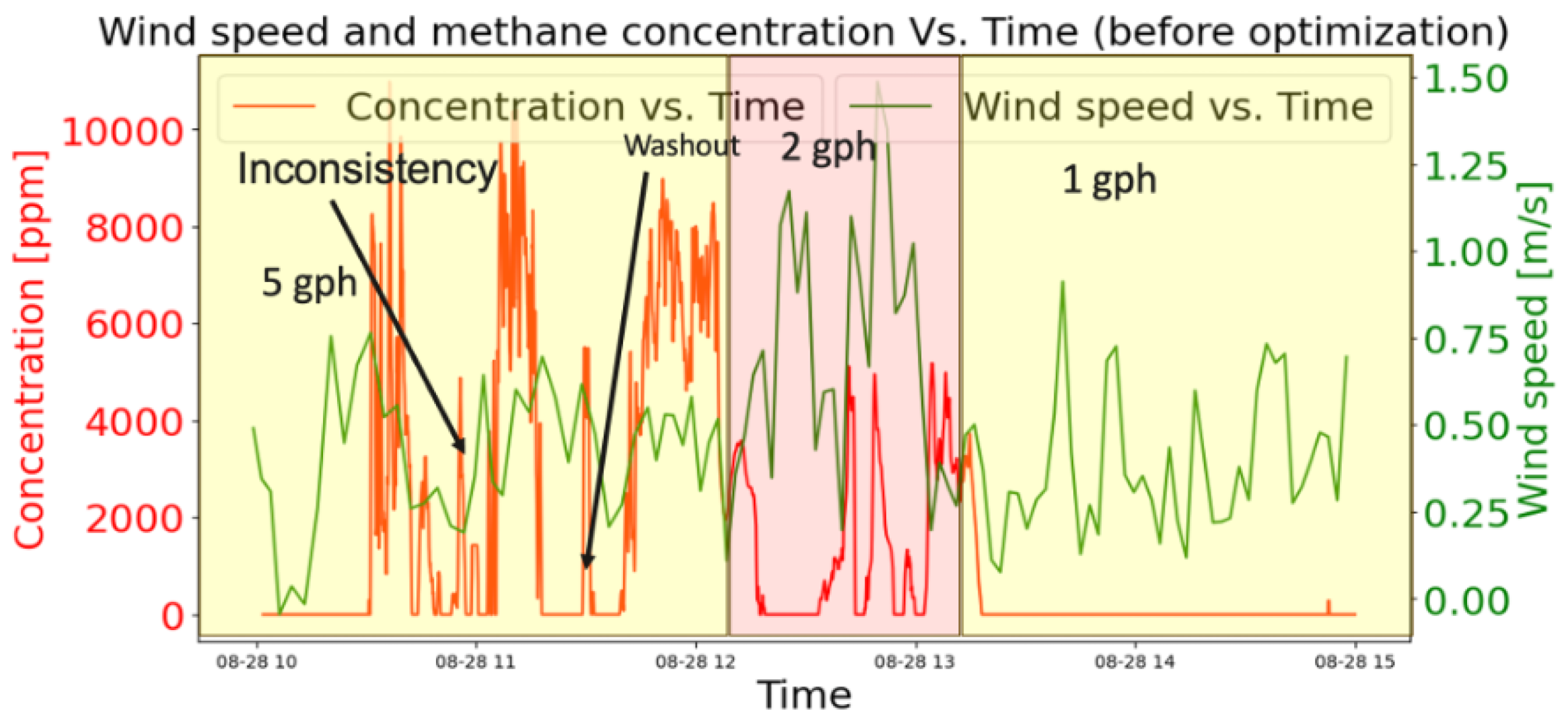
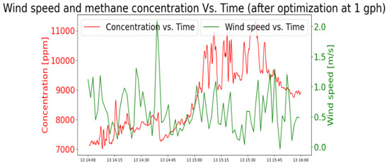
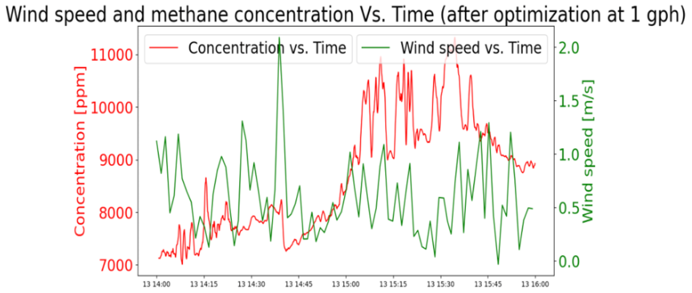
Washout happens when methane dilutes with air and falls below the sensor’s detection limit. After a washout, the methane concentration needs to build back up to reach a detectable limit again, which can leave some leak events undetected during the buildup process. Methane washout and signal fluctuation in the second design are visible in Figure 9, while the third design shows no evidence of washout and reduced fluctuation, as shown in Figure 10.
Figure 9.
Time-series methane concentration measurements from the second chamber design under varying leak rates, illustrating signal instability and washout behavior. As the leak rate decreases from 5 g/h to 2 g/h, the signal becomes increasingly intermittent and unstable, consistent with wind-driven dilution effects within the chamber. At 1 g/h, the methane concentration falls entirely below the sensor detection threshold, rendering the leak undetectable with this design.
Figure 10.
Methane concentration (red) and wind speed (green) time series for the third chamber design at a 1 g/h leak rate, recorded during controlled outdoor testing. Concentration remains consistently within the detection window (50–50,000 ppm) throughout the measurement period with no washout events observed.
3.2. Field Deployment Results
A third variation of the chamber was deployed on a plugged and abandoned well in the Los Angeles area. This test, which was redone multiple times, showed that recorded methane leaks have an intermittent pattern. This intermittency was initially expected by our research team when designing the chamber. It is important to note that the observed intermittency in the recorded data is influenced by multiple factors acting together: environmental conditions (temperature, pressure differences, and humidity fluctuations), changing wind speed and direction around the chamber opening, geological activities in the formations in contact with the well, and the deteriorating condition of the well itself. In the recorded data, temperature, pressure, and humidity showed no correlation with the observed leak patterns, but this does not exclude their contribution to short-term variability. A successfully plugged well should stop methane migration to the surface completely; the fact that the tested well exhibits detectable and repeated methane release indicates that its plugging integrity has been compromised, which is consistent with the 1951 partial cementing and wooden plug completion recorded for this well. Proving that any specific portion of the observed intermittency is attributable solely to well integrity, versus atmospheric or chamber effects, is not feasible with the static chamber design and uncontrollable wind conditions of this study. This limitation of interpretation is one of the reasons that motivated the shift toward time-series forecasting: rather than attributing individual intermittent events to specific causes, the forecasting model captures the overall statistical profile of the leak activity at the well, which can then be compared against follow-up deployments at the same site to assess changes over time.
Table 4 shows the statistical information about the recorded leak events. The first recorded leak event (154 ppm) was recorded 35 min after deployment began, with 93.1% of all recorded data showing zero concentration.
Table 4.
Statistical information of the recorded leak events on 20 September 2023.
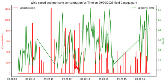
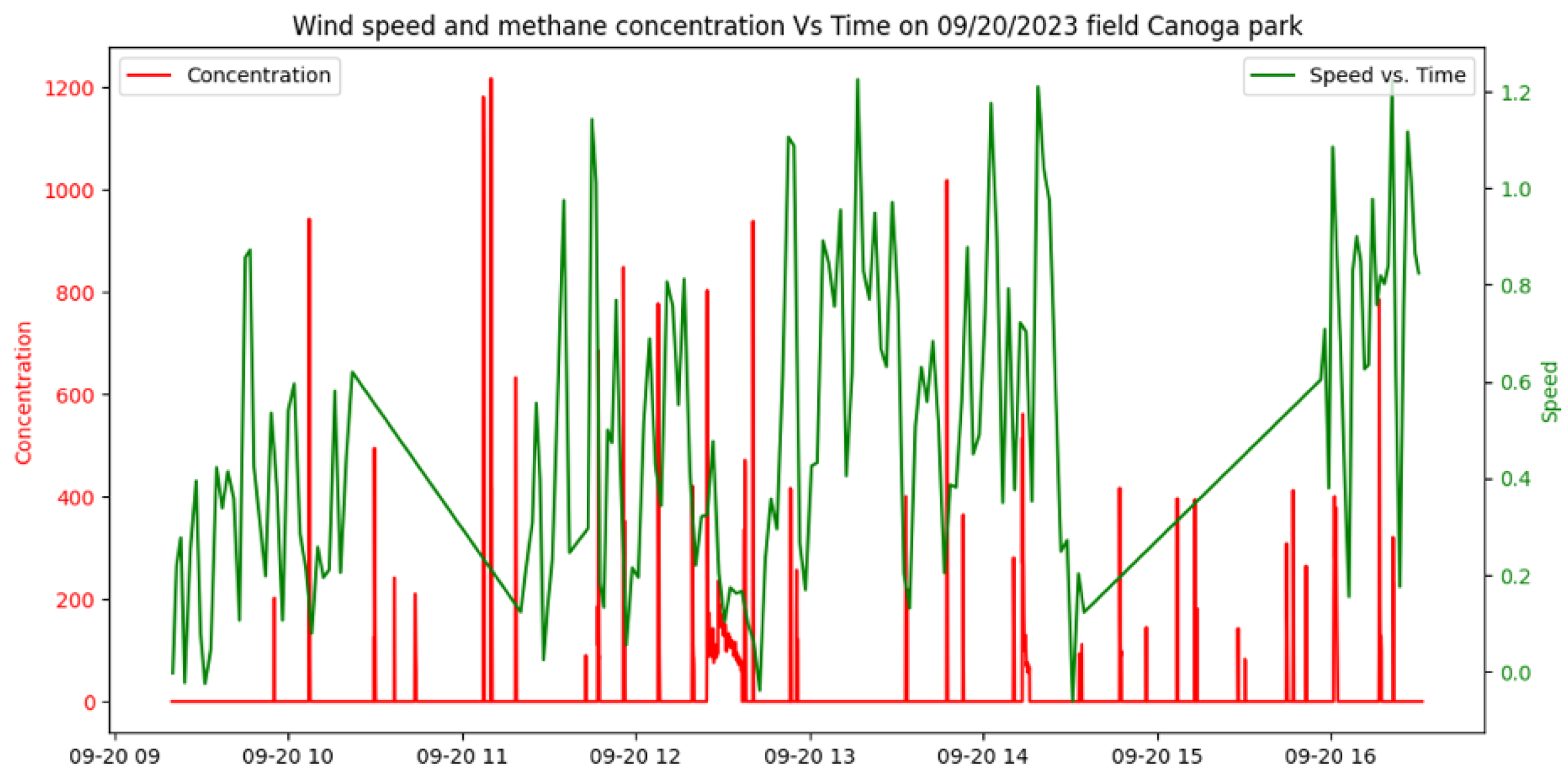
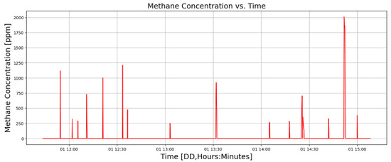
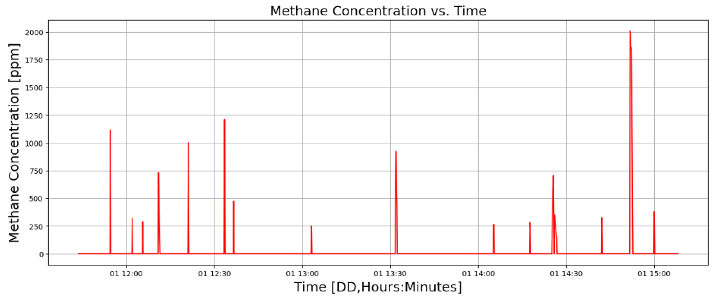
Results of the test conducted on 20 September 2023 are shown in Figure 11. During this test temperature changed between 22.77 and 38.94 centigrade. Another test conducted at the same location with the same configuration is shown in Figure 12, but this lacks wind data due to a technical failure of the wind sensor. These tests demonstrate the successful performance of the designed chamber in the field environment in detecting and monitoring methane emissions from plugged and unplugged wells.
Figure 11.
Methane concentration (red, left axis, ppm) and wind speed (green, right axis, m/s) recorded during the 20 September 2023 field deployment session at Canoga Park, spanning 7 h and 11 min from 09:19 AM to 4:31 PM. The co-plotted wind speed record demonstrates that emission spikes do not correlate consistently with any single wind speed condition.
Figure 12.
Methane concentration time series recorded during a 4 h field deployment session, showing highly intermittent emission spikes with no regular periodicity. Wind speed data are unavailable for this session due to a technical malfunction of the ultrasonic wind sensor. Peak concentrations exceeding 1000 ppm were recorded alongside extended periods of zero concentration, highlighting rapid mixing of methane and air.
3.3. Emission Forecasting Results
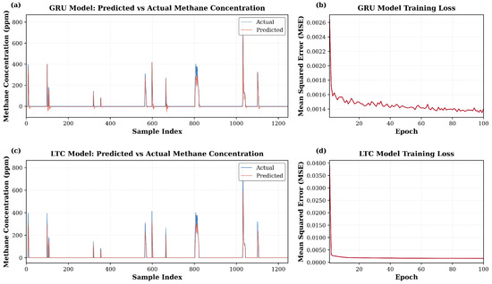
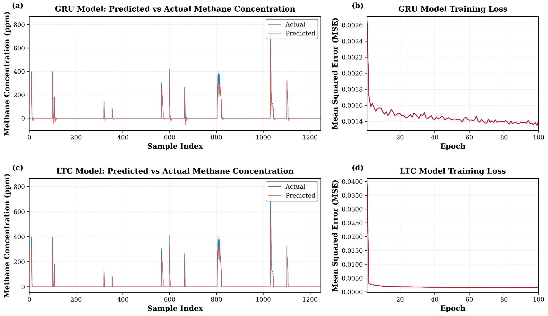
Performance of the two models used for time series forecasting of methane leak data is shown in Table 5, with LTC achieving a 2.7% better accuracy than GRU. Higher marginal accuracy of the LTC model came at a substantial computational cost (58-fold time difference). Leak event timing is predicted successfully, as shown in Figure 13 for both models. Undershooting of the predicted leak events is seen in both models, with predicted values averaging 15–25% below recorded leaks. In cases in which computational resources are limited, the GRU model can work ideally, but if the precision of the predictions is the priority, the LTC model is a better choice. Limited collected live data is one of the shortcomings of our models, which does not allow for the temporal and seasonal behavior of the leak profile.
Table 5.
Performance comparison of GRU and LTC forecasting models.
Figure 13.
Predicted (orange) versus measured (blue) methane leak event concentration on the held-out test set for the GRU (top) and LTC (bottom) models. Both models capture the timing and general pattern of intermittent emission events. Systematic under-prediction of peak concentrations (15–25% below measured values) is observed in both architectures. The LTC model achieves marginally lower prediction error (RMSE = 35.52 ppm, R2 = 0.6553) but reaches this error level earlier in training compared to GRU (RMSE = 36.49 ppm, R2 = 0.6362).
3.4. COMSOL-ML Optimization Results
3.4.1. Neural Network Accuracy
A recurrent neural network was trained to predict the fraction of observation points falling within each of the three concentration zones which are below detection, detection window or in range, and above LEL. The first detection window is between 50 ppm and 50,000 ppm (in range), and unsafe zones, which are above 50,000 ppm (above LEL), are considerably larger concentration ranges than the below-detection zone (<50 ppm), which causes greater variance in training targets and makes them inherently more challenging to predict accurately. In every simulation, 1000 observation points are placed inside the chamber to record the concentration in 1 min of transient simulation in 0.1 of a minute time steps. Recorded concentrations in each time step are used to train the neural network on the effect of each design parameter (methane leak rate, wind speed, chamber radius, chamber height, punched hole radius, well radius, and well height).
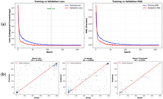
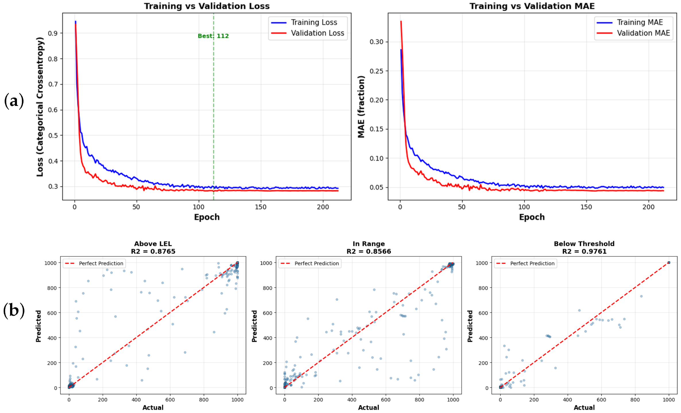
This is reflected in the test set performance reported in Table 6, where below-detection predictions achieved the highest accuracy. RMSE and MAE represent the average prediction error in the number of observation points (out of 1000) that were misclassified into the wrong concentration zone per simulation per timestep. The training achieved early stopping at 212 epochs, and its results are shown in Figure 14. Once trained, the surrogate model replaces direct COMSOL evaluation during optimization, reducing design computation time from approximately 6–8 h per simulation to 5–10 min for a complete optimization run.
Table 6.
RNN model test set performance. The splits are approximately 80% train, 10% validation, and 10% test (total of 228 simulations each containing 1000 observation points and 10 timesteps).
Figure 14.
RNN model training performance for all three concentration zone predictors: (a) training versus validation loss curves showing smooth convergence without overfitting, with dashed vertical lines indicating the best validation epoch for the model; (b) predicted versus actual scatter plots on the held-out test set, with dashed lines indicating perfect prediction.
3.4.2. Design Trade-Offs
This difference in optimization function weights produces two different sets of designs, as demonstrated in Table 7 for an example well with a radius of 0.07 m and height 0.3 m. The conservative design recommends a larger chamber radius (0.8675 m vs. 0.7322 m) and a taller chamber height (0.8614 m vs. 0.6397 m), providing a greater enclosed volume that reduces peak methane concentrations within the chamber. Conservative design lowers LEL risk from 1.1% to 0.9% at the cost of reducing detection coverage from 93.3% to 90.1%. The detection-optimized design achieves higher detection coverage by using a smaller, more compact chamber that keeps methane in the detectable range, reducing the below-detection percentage from 9% to 5.6%. The larger chamber volume in the conservative design allows more spacing for methane to disperse, which keeps concentrations within the safer but less detectable lower range. Operators with higher safety risk tolerance or working with wells exhibiting lower leak rates may prefer the detection-optimized design, while the conservative design is recommended for high-leak-rate scenarios or sites with limited ventilation. The surrogate model produces both designs in approximately 5 min, compared to the 6–8 h required per single COMSOL simulation on the same hardware [18 core Intel Xeon (R) CPU, 256 GB of RAM].
Table 7.
Example design recommendations for well radius = 0.07 m, well height = 0.30 m under worst-case wind and leak rate conditions.
4. Discussion
California had one of the biggest oil-producing fields, which caused an economic boom especially in Southern California, encouraging a mass number of individuals to move to California for better economic incentives. As cities in California expanded and productivity of the active fields declined over time, oil and gas assets were abandoned to end responsibility of the asset’s operators and to provide land for the rapidly expanding Southern California cities. Many of these wells were drilled and abandoned before modern abandonment regulations, and some have been left without any plugging and are now located underneath our homes, parks, parking lots, schools, and critical infrastructure such as ports and airports. Because these wells were abandoned without modern plugging techniques, open pathways are now available for crude and more importantly methane gas from these wells to leak to the surface.
Every year more operators in California and the United States leave their wells to become orphaned due to financial issues, which leaves states and the federal government responsible for the costly plug and abandonment that is not performed in a timely manner due to lack of funds and professional abandonment personnel. This issue continues to grow every year in size, leaving our communities at risk, while it adds to worsening global hazards of methane leaks as well.
Methane is a colorless and odorless gas with significant global warming potency, and could explode if it reached a lower explosive limit concentration. Several explosions have been tied to abandoned oil and gas wells, one of them being in Wheatley, which is located in Canada’s Ontario province. Since the methane leakage from these plugged and unplugged wells is reported to be intermittent with low leak rates, detection of these leaks is very challenging and costly through commonly used methane emission detection techniques such as thermal and lidar cameras or airborne monitoring systems. While wells that leak higher amounts of methane are discoverable with older techniques, many of the leaking assets are falsely flagged as non-leaking due to the shortcomings of technology and methane diluting with air immediately after release, leaving the concentration undetectable.
In this project a static flux chamber with an internet of things capability that records methane leak events from the plugged and unplugged Type 1 abandoned wells up to 1 g/h at a considerably lower cost was tested and designed. This was done by analyzing and processing recorded methane concentration, wind speed, pressure, temperature, and humidity from indoor and outdoor controlled tests so as to design the canopy to lower the methane and air dilution speed while leaving room for the canopy to be open to the atmosphere so the methane can leave the canopy area and not accumulate to dangerous concentration levels. This design was developed through extensive and iterative experiments that reduced the detection limit from 700 g in open air to 1 g/h. The trade off of safety and detectability is a multifaceted and complex engineering issue that was addressed in the chamber design. On the one hand, allowing more air to enter the chamber at higher speeds will cause the methane concentration to drop rapidly, which decreases the chance of detectability by the sensor; on the other hand, closing off the chamber and allowing less air to enter the chamber causes methane to build up in the chamber, making it potentially unsafe, and in the case of intermittent and low rate leaks allowing more methane to be absorbed by the soil at the bottom of the chamber. The sweet spot of the design parameters is where the risk tolerance and leak source behavior balance the trade off which can be handled by the design software. The software shows very high accuracy in predicting detectability and risk probability. The pipeline that was used in this section of the research can be expanded to match the specific needs of the operators.
The repeated field deployments showed an intermittent leak pattern, with 93.1% of recorded data showing zero concentration. A successfully plugged well should stop methane migration completely, so the detectable and repeated release from this well indicates compromised plugging integrity, consistent with its 1951 partial cementing and wooden plug completion. Under the reasonable assumption that formation pressure and available gas near the well are unchanged, the difference between predicted and newly recorded leak frequency and intensity in periodic re-deployments can indicate how the well’s condition has deteriorated over the elapsed period.
Both time-series prediction models predict leak timing successfully (LTC R2 = 0.6553 vs. GRU R2 = 0.6362) but show prediction undershooting by 15 to 25%, consistent with a model that has learned the average temporal pattern rather than memorizing individual extreme events. Because the goal is to capture the statistical profile of leak events for comparison against follow-up deployments, this under-prediction of extremes is acceptable and can be improved with more data collection. The LTC’s marginally higher accuracy came at a 58-fold computational cost, so the GRU is preferable when resources are limited and the LTC when prediction precision is the priority.
The canopy was deployed after extensive controlled tests on a plugged and abandoned well in the Los Angeles County which showed signs of fresh crude and gas leaks. After several deployments on this well site, the recorded dataset was used for AI-assisted time-series forecasting. This forecasting analysis helps extract the statistical profile of the methane leak for a well, allowing for periodic deployments instead of permanent installation. Periodic testing is a crucial capability of the canopy designed as it reduced theft risk, methane accumulation risk, and physical footprint on potentially thousands of wells that can be tested using this canopy. In addition to reducing the risks, periodic testing can answer the question of a well’s integrity declining rate with time. Cement-based plugging materials commonly used in oil and gas abandonment operations perform well at the time when the well is abandoned, but their integrity can be compromised with time due to tectonic movements and chemical reactions in the brine- and oil-bearing formations which cement and wells casing come in contact with. This has left a crucial question of how fast a plugged well’s integrity can be compromised, causing methane and crude to leak to the surface. This question can be answered using the designed canopy with time-series forecasting.
Plugged or unplugged abandoned wells can have different heights and diameters due to well-drilling time differences, targeted depths and socio-economic issues at the time of drilling or abandonment. These differences bring up an important question of what the physical design parameters of the canopy should ideally be to perform effectively in detectability and safety when well height and radius differ from one site to the other. The second important question is how a canopy can be designed to perform well in safely detecting methane leaks, as safety and detectability are two contradicting goals.
In Southern California many well sites are located under buildings or on privately owned land, which makes accessing them for testing challenging. In addition to the accessible sites issue, the methane leak rate and wind speed are the two main factors that a testing team has no control over during testing. Because of the mentioned issues, the ideal canopy shape based on the well height and radius can only be determined through computational fluid dynamics simulations. Some chambers use the controlled inflow of air or other gasses and measure the outflow of methane mixed with other gasses. The main aim of these chambers is to record the methane flow rate. The chamber designed in this study’s main aim is to record leak events from concentration levels (ppm) and does not tend to record flow rate. Using a gas container to establish a stable gas inflow will add major obstacles to the scalable solution that we had in mind, as the gas container is hard to move. Its volume is limited and may pose safety risks if left unattended in the field.
There are two main governing principles that a simulation of the canopy must account for. The first principle is advection force due to methane buoyancy and release and diffusion, which governs the general dispersion of methane into air. In the series of simulations conducted, laminar flow acts as the governing equation for the advection principle, and transport of concentrated species (TCS in COMSOL) accounts for the diffusion principle. The laminar flow equation is the Navier–Stokes equation and the TCS equation is a mass balance controlled by the binary diffusion coefficient of methane and air.
Real-world wind consists of local eddies and is multi-directional due to topographic and urban area effects, which makes the diffusion of methane and air much faster than a laminar flow. In the simulations, air flow is assumed to be laminar, which is a shortcoming because wind around the canopy structure reaches turbulent flow and it causes more pressure drops around the wind cap. A turbulent flow in the simulator is computationally very expensive (taking 10 times longer than a laminar flow), and it is much more likely not to converge by the end of simulation in a sweep simulation. The main goal of the simulation is to ensure the canopy is designed for safety, and since turbulent flow makes for faster methane and air dilution, it does not account for the most extreme and worst-case scenarios. Thus, a laminar flow was used instead of the turbulent flow for the air.
The next shortcoming of this methodology and system is that it has been designed to serve as the best possible system for Type 1 wells (according to the DOI guideline (2024) [1]), which means that the structure of the canopy is a rigid plastic-made structure. Abandoned wells come in different shapes and heights for which a rigid structure is not practically a suitable solution. Future research on non-rigid structure canopies can expand this work beyond Type 1 wells and fit different well sizes.
Due to resource limitations, no emergency vents were added to the canopy design. Vent locations and mechanisms can push the canopy shape focused on detectability, making the overall footprint and mobility of the canopy better. This project has been focused on establishing the methodology and shedding light on the physical principles important in methane air dilution modeling rather than producing a market-ready product. A market-ready product can benefit from emergency vents based on the operator and electricity resources of the well site.
The local wind sensor developed and used in this project malfunctioned in the field due to excessive heat and the physical shape of the wind sensor itself. Wind is one of the most important parameters in canopy design and the detection of methane leak events. As wind touches the sides of the canopy and its wind cap, it causes the Venturi effect. This effect causes methane to leak out of the canopy while wind is also entering the canopy and diluting the methane plume. A completely sealed canopy design was shown to perform poorly in methane emission detection as not enough buoyant forces are available between the leaked methane and air under the canopy to stop methane leakage from the canopy bottom and through the soil. The wind speed entering the canopy and the pressure drop caused by the wind at the canopy opening are the most important parameters in designing a canopy’s shape; thus, developing and using a wind sensor small enough to fit inside the wind cap can ensure that the overall design is based on accurately recorded wind speed.
Simulating outdoor and field wind speeds, especially under a turbulent regime, is very challenging unless the canopy structure and methane source are in a wind tunnel where wind speed and environmental conditions such as temperature and relative humidity can be fully controlled. Using laminar flow for the wind is one of the shortcomings. This shortcoming was realized by the research team during the simulation effort that could not be solved due to the high computation cost and because a laminar flow assumption will result in more extreme leak scenarios. Due to the limited resources and lack of experience in working with wind tunnels, the design of the canopy in this project was done without a wind tunnel.
The shortcomings of this canopy and the project mentioned above can be studied in future work. One of the most important future studies would be examining the canopy shape in a wind tunnel that can actively leak methane using a given frequency, which can shed light on the Venturi effect’s importance and also validate CFD simulations. Another important topic that can help in canopy design is studying the sinking effect of high-permeability loose soil where the canopy is deployed. Experimental results from our indoor, outdoor and field level tests in addition to Haase et al. (2025) [9] show that a considerable amount of gas can sink to the soil or leak from the canopy sides if the canopy is not buried in the soil or the soil is not wet. A sealing material that can be deployed on the canopy’s bottom can also increase methane detection performance.
Due to limited resources and the lead time required to source a suitable flow meter, no flow meter was installed inside the canopy to record the methane flow rate leaving it. Instead, an MPS methane sensor was used to record concentration during leak events, which can be complex and intermittent. Incorporating a flow meter in the canopy when a controllable wind source such as a wind tunnel is available can help build the right relationship between the leak rate, wind speed effect and concentration.
One of the main requirements of making this solution a scalable solution is reducing the cost of the detection system. Due to mechanical complexity and the need for personnel, previously proposed solutions had higher costs, which makes using them at scale challenging with the high number of potential leaking sources that are increasing every year. This canopy costs 250 US dollars (based on a September 2023 cost estimation by the research team) as a prototype with more than 80% of the cost allocated to the system’s sensor. The cost breakdown of the chamber is provided in the Supplementary Materials. The most affordable solution other than this canopy is marketed at USD 6000, which needs to be placed permanently at the well site, making an immobile and non-temporary solution. The cost of storing, analyzing and the communication of each canopy is calculated to be USD 8 per month per well if installed permanently. Research on using less expensive analogue methane emission detection sensors with a lower detection limit is currently going on at the USC Viterbi school of Engineering Electrical department, which can decrease the acquiring and prototype price of this canopy, making it a marketable and scalable solution.
Atmospheric and geographic conditions such as temperature, rain, humidity and accessibility in the oil and gas industry can pose problems for the systems that operate on valves, high pressure gas canisters, high-capacity batteries and any system that has complex mechanical components built into it. Operators need a user-friendly system that can be safely maintained in the field with basic tools and limited experience. Canopy design in this project incorporated the minimum number of components needed for a detection system to cover field conditions and operator’s resources. The lack of experienced personnel who need to be actively on site for the tests is one major issue that our designed canopy fixes with its IoT and real-time monitoring capability. Reducing the number of personnel needed per testing site reduces the funds needed for the methane emission detection of all plugged and unplugged wells significantly.
Because scalable solutions were not available to test a large number of wells with a standard method, existing data sets lack the size of tests conducted and confidence in accuracy. The designed canopy in this project expands the opportunity for testing a large number of wells with a standard testing protocol that can result in a comprehensive national and international data set which can later be used for data analysis tasks.
Many regulatory organizations and operators have limited resources to allocate across the many wells that require abandonment at a time; thus, a pre-screening solution using this canopy can help them allocate their limited resources to the wells that require the most attention faster than the ones that are not posing an immediate safety and financial risk. In the voluntary carbon credit markets, buyers are increasingly asking for long-term monitoring. The abandoned assets need to be monitored in a cost-effective, safe and easy-to-interpret way. This canopy also provides the right tool for this market as it can be permanently installed on an abandoned well.
The chamber developed in this study is designed for Type 1 wells based on the DOI methane measurement guidelines [6]. Type 1 wells, by definition, only have a limited small structure at the surface that can easily be covered by a portable chamber. Wells that are not plugged and abandoned, idle, or orphaned typically have a production line connected to them, or they are larger in height and radius with a wellhead assembly attached. Such configurations cannot practically fit under a flux chamber of the rigid design used in this study. Future research on flexible, non-rigid structure canopies can extend this work beyond Type 1 wells and accommodate larger wells across all categories. Validation of the chamber and the forecasting models was constrained by the limited number of wells accessible for testing. In California, the majority of plugged and abandoned wells are located on privately owned land and are not accessible to the public, which restricted field deployment in this study to a single publicly accessible Type 1 well site. Expanding validation to additional wells across multiple geographic regions and well types is a priority for future work and will require partnerships with state regulatory agencies and private landowners to gain access. Independent deployment sessions on additional wells would also strengthen the assessment of the forecasting models’ generalization beyond the single well used for training in this study.
This manuscript integrates the prior chamber design iterations, field deployment results, and computational fluid dynamics work into a single unified framework with new outdoor testing iterations, time-series forecasting, and machine learning-based design optimization not included in those earlier publications.
5. Conclusions
Using this canopy and incorporating future studies on methane emission detection from plugged, unplugged, orphaned, and abandoned wells can ensure the safety of communities in proximity to historical well sites, improve methane emission inventory accuracy, and enable states and the federal government to allocate funds efficiently and in a timely manner. The urgency of these efforts is reinforced by recent analysis from Purvis (2026) [16], which estimates that between 4.4 and 5.7 million onshore oil and gas wells exist in the United States, with 142,000 currently classified as orphan wells and an additional 2.7 to 3.2 million wells at risk of becoming wards of the state in the future through either operator bankruptcy or post-plugging leakage and best technologies and practices review by the National Academies of Science, Engineering and Medicine (2026) [17].
Supplementary Materials
The following supporting information can be downloaded at: https://www.mdpi.com/article/10.3390/environments13070411/s1, S1: Mesh Independence Study including parameters, results table, and discussion of mesh convergence.
Author Contributions
N.D. is the lead researcher of this project in experimental, artificial intelligence and computational fluid dynamic simulations tasks. Y.P.G. assisted with the time series prediction modeling task. Y.C. is the lead scientist behind sensor and communication kit development. R.K. has been the supervisor behind artificial intelligence models. S.F., I.E. and D.P. have been supervising all of the project steps. All authors have read and agreed to the published version of the manuscript.
Funding
This research was funded by Beyond Limits, University of Southern California and Ershaghi Center for Energy Transition.
Institutional Review Board Statement
Not applicable.
Data Availability Statement
All source code, trained machine learning model weights, and simulation configuration files generated during this study are publicly available at the StaticFlowChamber repository [https://doi.org/10.5281/zenodo.19770457]. Experimental calibration data, field deployment records, and full COMSOL simulation datasets are available from the corresponding author upon reasonable request, as file sizes exceed repository storage limitations.
Acknowledgments
The authors gratefully acknowledge the Ershaghi Center for Energy Transition at the University of Southern California and Beyond Limits for providing the platform and resources for this research. We also acknowledge Pooya Khodaparast, Cyrus Ashayeri, and Tedrik Hayrapetian for their mentorship and efforts in this research. During the preparation of this manuscript, the authors used Claude (Anthropic, Claude Opus 4.7) for manuscript conversion from Microsoft Word to LaTeX format, grammar and language editing, and code debugging. The authors have reviewed and edited the output and take full responsibility for the content of this publication.
Conflicts of Interest
Shahram Farhadi was employed by Beyond Limits at the time when project was ongoing and is an employee of Ensense AI during the preparation of this article. The authors declare that this study received funding from Beyond Limits. The funder was not involved in the study design, collection, analysis, interpretation of data, the writing of this article, or the decision to submit it for publication.
Abbreviations
The following abbreviations are used in this manuscript:
| CFD | Computational fluid dynamics |
| DOI | Department of the Interior |
| GRU | Gated Recurrent Unit |
| IoT | Internet of Things |
| LEL | Lower explosive limit |
| LHS | Latin Hypercube Sampling |
| LTC | Liquid Time-Constant |
| ML | Machine learning |
| PPM | Parts per million |
| SPE | Society of Petroleum Engineers |
| RNN | Recurrent neural network |
References
- U.S. Department of the Interior, Orphaned Wells Program Office. FY 2024 Orphaned Wells Program Annual Report to Congress; U.S. Department of the Interior: Washington, DC, USA, 2024. Available online: https://www.doi.gov/sites/default/files/documents/2024-11/fy-2024-owpo-annual-congressional-reportfinal-publishing.pdf (accessed on 18 February 2026).
- Townsend-Small, A.; Ferrara, T.W.; Lyon, D.R.; Fries, A.E.; Lamb, B.K. Emissions of Coalbed and Natural Gas Methane from Abandoned Oil and Gas Wells in the United States. Geophys. Res. Lett. 2016, 43, 2283–2290. [Google Scholar] [CrossRef] [Scilit]
- California Council on Science and Technology. Orphan Wells in California: An Initial Assessment of the State’s Potential Liabilities to Plug and Decommission Orphan Oil and Gas Wells; CCST: Sacramento, CA, USA, 2020; Available online: https://ccst.us/wp-content/uploads/CCST-Orphan-Wells-in-California-An-Initial-Assessment.pdf (accessed on 18 February 2026).
- Kang, M.; Kanno, C.M.; Reid, M.C.; Zhang, X.; Mauzerall, D.L.; Celia, M.A.; Chen, Y.; Onstott, T.C. Direct Measurements of Methane Emissions from Abandoned Oil and Gas Wells in Pennsylvania. Proc. Natl. Acad. Sci. USA 2014, 111, 18173–18177. [Google Scholar] [CrossRef] [Scilit] [PubMed]
- Dubey, L.; Cooper, J.; Hawkes, A. Minimum Detection Limits of the TROPOMI Satellite Sensor across North America and Their Implications for Measuring Oil and Gas Methane Emissions. Sci. Total Environ. 2023, 872, 162222. [Google Scholar] [CrossRef] [Scilit] [PubMed]
- U.S. Department of the Interior, Orphaned Wells Program Office. Assessing Methane Emissions from Orphaned Wells to Meet Reporting Requirements of the 2021 Infrastructure Investment and Jobs Act: Methane Measurement Guidelines; U.S. Department of the Interior: Washington, DC, USA, 2023. Available online: https://www.doi.gov/sites/default/files/orphaned-wells-methane-measurement-guidelines-july-2023-version.pdf (accessed on 15 July 2026).
- Qi, Q.; Khoja, G.; Ershaghi, I. Reservoir Engineering and Geomechanical Aspects of Well Plugging and Abandonment. In Proceedings of the SPE Middle East Oil & Gas Show and Conference, Manama, Bahrain, 28 November–1 December 2021. [Google Scholar] [CrossRef] [Scilit]
- Riddick, S.N.; Mauzerall, D.L.; Celia, M.A.; Kang, M.; Bandilla, K. Variability Observed over Time in Methane Emissions from Abandoned Oil and Gas Wells. Int. J. Greenh. Gas Control 2020, 100, 103116. [Google Scholar] [CrossRef] [Scilit]
- Haase, K.B.; Gianoutsos, N.J. Evaluating Mass Flow Meter Measurements from Chambers for Greenhouse Gas Emissions from Orphan Wells and Other Point Sources. Atmos. Meas. Tech. 2025, 18, 4207–4226. [Google Scholar] [CrossRef] [Scilit]
- NevadaNano. MPS Methane Gas Sensor Brochure; Nevada Nanotech Systems Inc.: Sparks, NV, USA, 2021; Available online: https://nevadanano.com/wp-content/uploads/2021/09/NN_Brochure_MethaneSept2021•DIGITAL.pdf (accessed on 2 July 2026).
- NevadaNano. MPS Methane Gas Sensor Online Brochure; MPS flammable gas sensor specification; Nevada Nanotech Systems Inc.: Sparks, NV, USA, 2026; Available online: https://nevadanano.com/products/mps-flammable-gas-sensor/ (accessed on 2 July 2026).
- Hasani, R.; Lechner, M.; Amini, A.; Rus, D.; Grosu, R. Liquid Time-Constant Networks. In Proceedings of the AAAI Conference on Artificial Intelligence, Virtual, 2–9 February 2021; Volume 35, pp. 7657–7666. [Google Scholar] [CrossRef] [Scilit]
- Hasani, R.; Lechner, M.; Amini, A.; Liebenwein, L.; Ray, A.; Tschaikowski, M.; Teschl, G.; Rus, D. Closed-Form Continuous-Time Neural Networks. Nat. Mach. Intell. 2022, 4, 992–1003. [Google Scholar] [CrossRef] [Scilit]
- Burgess, D.R. NIST Technical Note 2279; National Institute of Standards and Technology: Gaithersburg, MD, USA, 2024. Available online: https://nvlpubs.nist.gov/nistpubs/TechnicalNotes/NIST.TN.2279.pdf (accessed on 12 March 2025).
- Karim, G.A.; Lam, H.T.; Petela, R.; Rowe, R. Experimental and Analytical Investigation of the Convective Diffusion of Methane Into Air. J. Energy Resour. Technol. 1987, 109, 230–234. [Google Scholar] [CrossRef] [Scilit]
- Purvis, D. Impending Risk of Orphaning: The Number and Status of Onshore U.S. Oil and Gas Wells; Purvis Energy Advisors: Fort Worth, TX, USA, 2026; Available online: https://www.purvisenergyadvisors.com/impending-risks-landing-page (accessed on 19 June 2026).
- National Academies of Sciences, Engineering, and Medicine. Technologies and Practices for Plugging and Remediating Orphan Oil and Gas Wells; The National Academies Press: Washington, DC, USA, 2026. [Google Scholar] [CrossRef] [Scilit] [PubMed]

Disclaimer/Publisher’s Note: The statements, opinions and data contained in all publications are solely those of the individual author(s) and contributor(s) and not of MDPI and/or the editor(s). MDPI and/or the editor(s) disclaim responsibility for any injury to people or property resulting from any ideas, methods, instructions or products referred to in the content. |
© 2026 by the authors. Licensee MDPI, Basel, Switzerland. This article is an open access article distributed under the terms and conditions of the Creative Commons Attribution (CC BY) license.