


Abstract
Landfills are important sources of particulate matter emissions (PM10 and PM2.5) generated by heavy machinery, vehicle traffic and particle resuspension. This study aimed to assess the dispersion of PM10 and PM2.5 at a Mexican sanitary landfill by coupling mathematical modeling with field monitoring. Using site-specific operational data and five years of meteorological data from the Toluca 76675 station (2021–2025), emission rates were estimated with the US EPA AP-42 emission factors for unpaved roads, aggregate handling and storage piles, and industrial wind erosion. Atmospheric dispersion was then simulated with the AERMOD modeling system on a grid of 100 × 100 receptors with 50 m spacing (4.95 km × 4.95 km). Field monitoring was conducted for one year at nine strategic points within the landfill with portable optical particle counters (Dust Particle Counter TC-8100), three days per week during the 12 h operating shift. In situ monitoring recorded the highest values at the excavation zone (PM10: 225.23 µg/m3; PM2.5: 173.08 µg/m3) and at the active working face (PM10: 212.43 µg/m3; PM2.5: 200.61 µg/m3), as annual averages of the operating shift; these concentrations exceed the WHO ambient air quality guideline values, although they are below the occupational exposure limits of NOM-010-STPS-2014. The model indicates that the plumes are oriented toward the SW and that the highest concentrations are located over the unpaved access road, the dominant source in the inventory.
1. Introduction
1.1. Particulate Matter Emissions at Waste Disposal Facilities
The World Bank reports that global municipal solid waste (MSW) generation reached 2.6 billion tons in 2022 and, more worryingly, is projected to reach 3.9 billion tons by 2050, a 50% increase between 2022 and 2050 [1,2]. This growth in waste volume not only represents a management challenge but also aggravates the environmental problems associated with final disposal. This last stage is an important source of particulate matter emissions to the atmosphere through multiple activities that release these pollutants: the daily operation of heavy machinery, the constant traffic of waste collection vehicles, wind-driven resuspension of particles from exposed surfaces and, in many cases, accidental or controlled fires [3]. Thus, an increase in the amount of waste disposed of implies more collection-vehicle trips, more material handled and larger exposed surfaces, which are precisely the activity variables that determine particle emissions in the US EPA estimation methods [4].
Particulate matter has potential impacts on air quality and on the health of nearby populations [5]. Particles smaller than 10 µm and 2.5 µm, PM10 and PM2.5, are of particular concern because they can penetrate deep into the respiratory system and reach the bloodstream, and because of their association with cardiovascular, respiratory and neurological diseases [6,7]. Particulate matter is a mixture of solid and liquid particles suspended in air; PM10 and PM2.5 correspond to the fractions with an aerodynamic diameter less than or equal to 10 and 2.5 µm, respectively. In addition to final disposal sites, their main sources are combustion in vehicles and industry, biomass burning, and dust resuspension from roads and from construction and mining activities. The World Health Organization (WHO) sets recommended short-term (24 h) air quality guideline levels for particulate matter of 45 µg/m3 for PM10 and 15 µg/m3 for PM2.5 [8]. These air quality levels are necessary to protect public health worldwide [9]. In Mexico, NOM-025-SSA1-2021 sets 24 h limit values of 70 µg/m3 for PM10 and 41 µg/m3 for PM2.5, and annual values of 36 and 10 µg/m3, respectively; compliance is assessed with 24 h averages obtained from continuous measurements in air quality monitoring networks [10].
In Mexico, challenges persist in the disposal of MSW at uncontrolled sites, controlled sites and sanitary landfills, where limited infrastructure and operational deficiencies can intensify pollutant emissions [11]. To understand the actual extent of the impact on the environment and on the health of nearby communities, the dispersion of PM10 and PM2.5 within and around final disposal sites must be assessed. However, quantitative information on air quality at these sites is scarce: the studies available in Mexico have focused on fire episodes [5] or on assessments of the environmental impacts of the site as a whole [11] and, to the best of our knowledge, no year-long monitoring campaigns inside operating sanitary landfills, or evaluations of dispersion model performance against on-site measurements, have been published. This lack of information limits the ability of environmental authorities to implement effective mitigation measures and to design risk-based response protocols. This information is relevant not only to the exposed population but also to the workers who carry out their daily tasks on site. Although Mexico has a regulatory framework for the prevention of occupational risks, such as NOM-017-STPS-2008 and NOM-030-STPS-2009 [12,13], the consistent application of these standards remains a challenge. The documented exposure of Mexican landfill workers to respiratory diseases and skin complications reveals a substantial gap between regulations and their effective implementation [14]; measures should therefore be proposed to reduce the risk of occupational diseases and to contribute to workforce sustainability and to the social responsibility of landfill operators [15,16].
1.2. Tools for Assessing Airborne Particulate Matter
To verify regulatory compliance and assess air quality in real time, various field instruments are used, such as portable particle counters, including the PCE-MPC 10, the Purple Air PIXEL BMV080, the Pollusense, Graywolf instruments and the Temtop PMD 351 [17,18,19], which allow in situ monitoring of PM2.5 and PM10 concentrations through direct and continuous measurements, facilitating the identification of emission sources. Another indispensable tool is atmospheric dispersion modeling, which makes it possible to assess the territorial and environmental impact of emissions by simulating the dispersion of pollutants in space and time, integrating meteorological, topographic and operational variables within a mathematical framework [20,21]. Several modeling programs exist, such as the California PUFF Model, the Atmospheric Dispersion Modelling System, the Community Multiscale Air Quality model and AERMOD [22]. These models differ in their formulation and scale of application: CALPUFF is a Lagrangian puff model suited to transport over distances of tens to hundreds of kilometers and to complex wind fields; CMAQ is a regional-scale Eulerian photochemical model whose cells of several kilometers do not resolve the near field of a source; ADMS and AERMOD are steady-state Gaussian models based on boundary layer theory, designed for distances of up to 50 km. AERMOD was selected in this study because it is the US EPA preferred model for the near field, includes algorithms for area sources and for terrain effects (through AERMAP), and is the most widely used model in assessments of final disposal sites, which facilitates the comparison of results [23]. AERMOD is the model recommended by environmental agencies such as the United States Environmental Protection Agency (EPA). It simulates pollutant behavior under different meteorological (wind speed and direction, atmospheric stability, temperature) and topographic (flat or complex terrain) conditions and generates surface concentration maps resulting from the modeled dispersion processes [22,23]. AERMOD has been used in research on pollutant dispersion at sanitary landfills and uncontrolled sites, such as the study by Jawwad et al. [16] at the TPA Klotok landfill in Kediri, Indonesia, which found a rapid decrease in PM10 and PM2.5 concentrations beyond 100 m from the dump, as well as in impact analyses on receptor communities in Nigeria [24]. In these studies, concentrations depend mainly on traffic intensity on unpaved roads, on the silt and moisture content of surfaces, and on wind speed and atmospheric stability, which control both emission and dilution [4,24,25].
The objective of this study was to assess the dispersion of PM10 and PM2.5 emitted at the Zinacantepec Integrated Waste Center (IWC), Mexico, by combining an AP-42-based emission inventory, AERMOD modeling and on-site field monitoring. Specifically, we sought to: (i) describe the spatial pattern of dispersion of the site emissions and identify the zones of highest concentration; (ii) characterize PM10 and PM2.5 concentrations at the monitoring points during the operating shift; (iii) identify the sources with the largest contribution in the emission inventory; and (iv) estimate worker exposure. The contribution of this study lies not in the tools, which are well established, but in providing one year of measurements inside an operating sanitary landfill in a middle-income country and in identifying, by contrasting them with the AP-42/AERMOD approach, the limitations of this approach and the requirements for applying it, particularly for the fine fraction.
2. Study Area
The final disposal site selected as the study area was the Zinacantepec site, located in Paraje Tepetatal (geographic coordinates: 19.327999713499576, −99.7725206978884), at 2764 m a.s.l. [26], in the SW part of the State of Mexico. According to the Consultation Portal of the Integrated Waste System of the State of Mexico, it is registered as an IWC and covers a total area of 213,525.69 m2. The site hosts various facilities and operating systems for MSW management and treatment, including a vermicomposting system to treat the organic fraction, eleven final disposal cells built according to the guidelines of the Mexican Official Standard NOM-083-SEMARNAT-2003, a biogas capture and control system consisting of 53 venting wells, and a set of six stabilization ponds for the management and containment of the leachate generated [27,28].
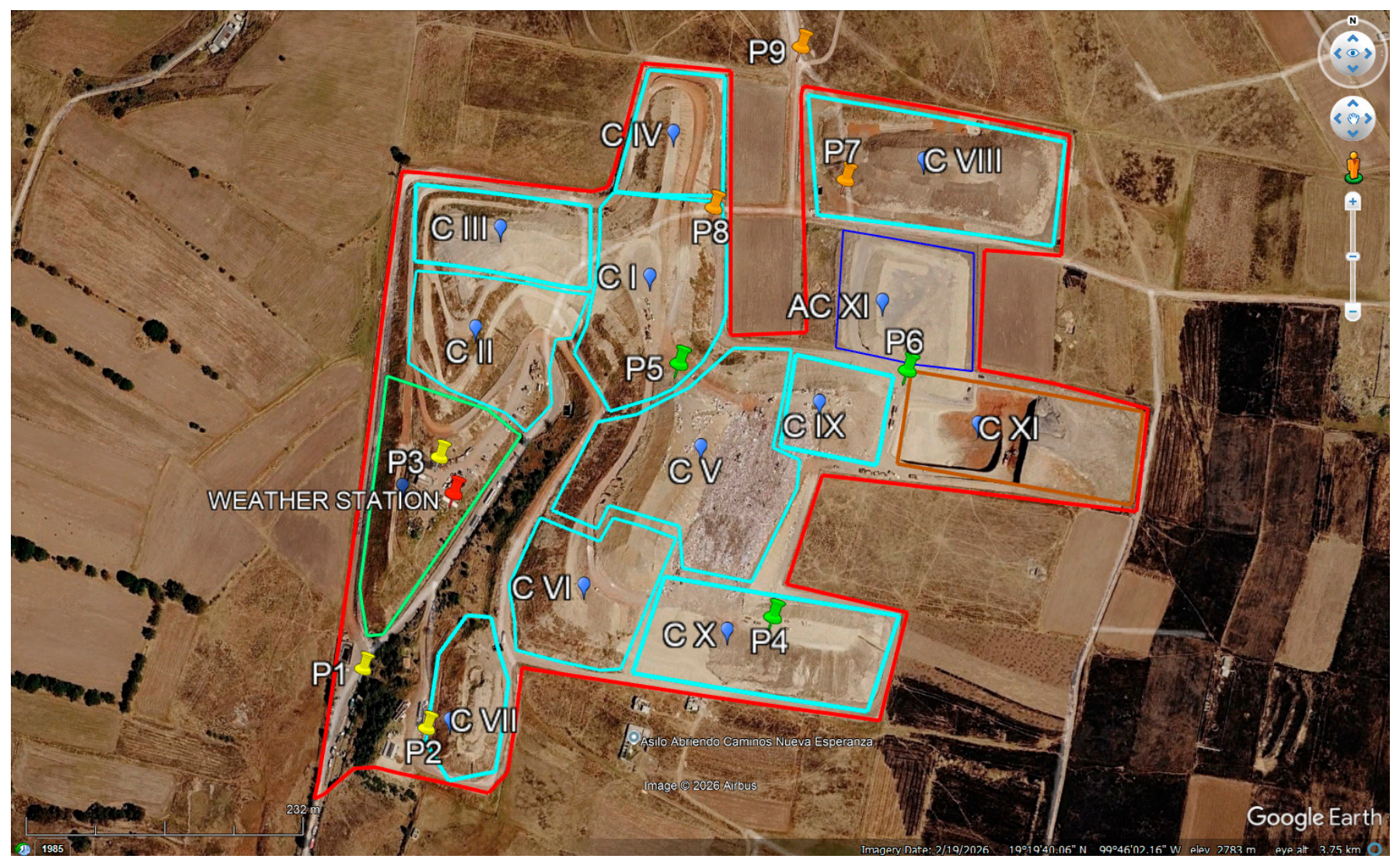
Notably, the Zinacantepec IWC is intermunicipal, as it provides final disposal services to a total of 12 adjacent and neighboring municipalities, which underlines its relevance in regional waste management. Based on its operating capacity and the volume of waste it receives, the site is classified as a type A final disposal site, since it receives on average 1352 t/d (Table 1). In Figure 1, the shaded areas correspond to: closed cells I to X (cyan); active cell XI, where the working face is located (brown); cell expansion, AC (blue); remediated cell, Cs (green); the numbered symbols indicate the monitoring points P1–P9, and the red symbol indicates the location of the meteorological station. Waste is currently deposited exclusively in Cell XI, during a single daily 12 h operating shift.
Table 1.
Data collected on landfill operation.
Figure 1.
Location and layout of the facilities of the Zinacantepec IWC (State of Mexico).
3. Materials and Methods
To meet the objectives of the study, a methodology structured in sequential phases was implemented, integrating the collection of primary and secondary information (meteorological, topographic and site operation data), atmospheric modeling of emission rates and particle dispersion, field monitoring of particulate matter and a comparative analysis of the results.
3.1. Meteorological and Topographic Data
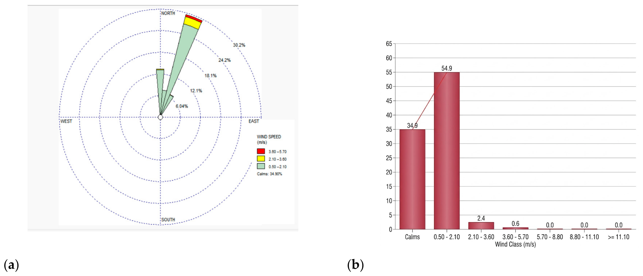
The modeling used the surface and upper-air (radiosonde) meteorological files of the Toluca station (Toluca station 76675) for the period from 1 January 2021 to 31 December 2025 (five years of hourly data), processed with AERMET; surface characteristics were estimated with AERSURFACE from the surrounding land use (albedo of 0.6, Bowen ratio of 2.0 and surface roughness length of 0.1 m) [22]. The wind rose and the wind speed frequency distribution (Figure 2) were prepared with WRPLOT View (Version 8.0, Lakes Environmental Software, Waterloo, ON, Canada) from the same data. In addition, the DAVIS Vantage Vue (Davis Instruments, Hayward, CA, USA) station installed on the roof of the IWC administrative offices, about 12 m above ground level, recorded local conditions during the monitoring period.
Figure 2.
(a) Annual wind rose (petals indicate the direction from which the wind blows) and (b) wind speed frequency distribution, prepared with WRPLOT View from the hourly data of the Toluca station (2021–2025) used in AERMOD.
Topographic and terrain elevation data were obtained from the Digital Elevation Models of the National Institute of Statistics and Geography (INEGI) [29]. Specifically, vector and raster data layers covering the IWC area of influence were used, with a spatial resolution of 15 m (scale 1:50,000). This information was processed with geographic information systems, such as the State of Mexico Atlas Viewer and the INEGI Digital Map, to characterize the surrounding topography (Figure 3); source and receptor elevations in AERMOD were obtained with AERMAP from the SRTM3 digital elevation model.
Figure 3.
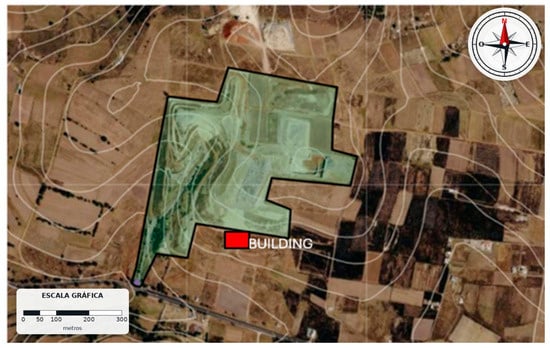
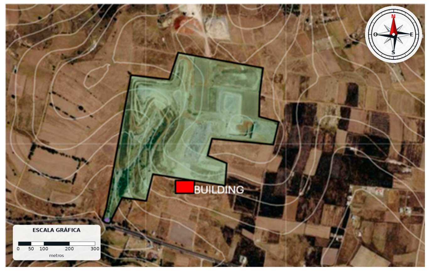
Topography around the Zinacantepec IWC: contour lines obtained from the INEGI digital elevation model (15 m resolution), IWC boundary (black line) and the nearest building in the SW sector (red box).
3.2. Landfill Operation Data
The site activity data needed to estimate emissions were obtained through a one-year in situ survey, with the support of the landfill operating staff, who record at the weighbridge the types and number of incoming vehicles and the amount of waste they carry. Vehicles were classified as: (i) municipal collection vehicles (two-axle compactor trucks), (ii) private vehicles and (iii) heavy-duty vehicles (trailers and dump trucks). For each category, the route traveled within the IWC was documented, including the distances traveled on unpaved roads (from the entrance to the final disposal cell). The fuel used by each vehicle type was investigated, and the IWC administration provided information on the technical specifications of the vehicle fleet and machinery (backhoes and compactors).
The MSW from the active cell was physicochemically characterized following the methodology reported by Hernández-Contreras et al. (2026) [30], also determining the moisture content of the fine fraction, since this parameter is relevant for assessing waste behavior during degradation and its possible influence on the generation of gaseous and particulate emissions. The road soil and the cover material of the closed cells were characterized according to the standards NMX-AA-015-1985, NMX-AA-022-1985 and NMX-AA-016-1984 [31,32,33,34,35,36].
3.3. Estimation of Particle Emission Rates
The main particle emission sources considered were waste transport operations, handling and unloading operations, and the diffuse release of particles by wind erosion of unvegetated surfaces. PM10 and PM2.5 emission factors were obtained following the methodology of the EPA Compilation of Air Pollutant Emission Factors (AP-42) [4]. For the sources associated with waste transport, Chapter 13 (“Miscellaneous Sources”) was used, specifically Section 13.2.2 for unpaved roads, which provides Equation (1), adapted to metric units (g per vehicle-kilometer traveled, g/VKT).
where k is the particle size multiplier (42.3 g/VKT for PM2.5 and 422.8 g/VKT for PM10, equivalent to 0.15 and 1.5 lb/VMT for industrial unpaved roads), s is the silt content in the AP-42 sense, i.e., the fraction of surface material passing a No. 200 sieve (<75 µm), determined by sieving road surface samples according to AP-42 Appendix C [4] (%), W is the mean fleet weight in short tons (13.5 t = 14.9 short tons), and the exponents a and b take values of 0.9 and 0.45, respectively (AP-42 Table 13.2.2-2). Emissions from the handling and storage of waste and other aggregate materials (such as material piles, MSW movement and the cover material used at the IWC) were estimated with Equation (2), based on the methodology of Section 13.2.4 (“Aggregate Handling and Storage Piles”).
where E is the emission factor (kg per tonne of material handled), k is the particle size multiplier (0.053 for PM2.5 and 0.35 for PM10, which multiply the constant 0.0016), U is the wind speed (m/s), M is the material moisture content (%), and the exponents of the wind speed and moisture terms take values of 1.3 and 1.4, respectively. This equation accounts for both emissions from material drop during loading and unloading operations and emissions from wind resuspension. Total aggregate handling emissions were calculated by multiplying the emission factor by the amount of material handled daily (Mmat), expressed in t/d, using Equation (3).
Wind-driven fugitive particulate emissions from the exposed surfaces of the site (inactive cells and areas without vegetation cover) were quantified with the methodology of Section 13.2.5 (“Industrial Wind Erosion”). Following AP-42, the erosion potential P (g/m2) of each surface disturbance was estimated as P = 58 (u* − u*t)2 + 25 (u* − u*t) for u* > u*t (P = 0 otherwise), where u* is the friction velocity (m/s), obtained from the maximum (fastest-mile) wind speed at 10 m (u* = 0.053 u+10), and u*t is the threshold friction velocity of the material (0.28 m/s); the emission is obtained as E = k Σ Pi, with k = 0.5 for PM10 and 0.075 for PM2.5 (Equation (4)) [4].
where Ee is the emission per unit area (g/m2) and Pi is the erosion potential of each surface disturbance during the period considered. Total wind erosion emissions (Ee) were obtained by multiplying the emission factor by the exposed area (Aexp) in m2 (Equation (5)):
Once the emission factor (E) of each equation had been estimated, the total daily emission (M) was calculated with Equation (6).
where N is the number of daily trips and Lkm is the distance traveled in km.
Finally, to obtain the area emission rate (Q) required by AERMOD for area sources, Equation (7) was applied.
where Mkg/d is the daily emitted mass in kg/day, Tact is the daily activity time in seconds (considering 12 h of operation) and is the source area in m2.
The correspondence between activities and emission factors was as follows: (i) Section 13.2.2, vehicle traffic on the internal unpaved roads, represented in the model by two polygons (E1 and E2; 43,686 m2 in total) along which P1, P2, P3, P5 and P8 are located; the number of trips and the vehicle type were obtained from the daily weighbridge records, the mean fleet weight from the technical specifications provided by the IWC administration, and the distance traveled per trip was measured along each route with a geographic information system; (ii) Section 13.2.4, excavation (D, P4; 9504 m2), cover-material borrow area (I, P9; 10,671 m2) and MSW unloading and spreading at the working face (F, P6; 9720 m2), with the amount of material handled obtained from the weighbridge records and machinery logs and the moisture content from the characterizations described in Section 3.2; for the working face, the estimated emission was negligible (1.0 × 10⁻¹² g/(s·m2)) owing to the moisture content of the MSW, so it was entered into the model as zero; and (iii) Section 13.2.5, wind erosion of the remediated cell (G, P7; 21,265 m2), whose area was delineated on an orthophoto and for which only the PM10 emission was estimated. The service areas (P1–P3) and the pumping sump (P8) were included in the model only as references, without emissions. Exhaust emissions from diesel vehicles and machinery and traffic on the working face were not included in the inventory, as discussed in Section 4.7.
3.4. Modeling of PM10 and PM2.5 Dispersion
Using the IWC-specific emission factors and activity data, the dispersion of PM10 and PM2.5 was modeled with AERMOD (version 24142; U.S. Environmental Protection Agency, Research Triangle Park, NC, USA) through the AERMOD View interface (version 13.0.0; Lakes Environmental Software, Waterloo, ON, Canada), with the default regulatory options, rural dispersion coefficients and elevated terrain. Each activity was represented as a polygonal area source (AREAPOLY) whose geometry matches the surface on which it takes place (Table 2), with a release height of 0 m. Concentrations were calculated on a uniform Cartesian grid of 100 × 100 receptors with 50 m spacing (4.95 km × 4.95 km), at a height of 1.2 m above ground; no discrete receptors were defined at the monitoring points. The dry and wet deposition and plume depletion options were not activated. Emission rates, calculated for the 12 h operating shift (Equation (7)), were applied constantly over the 24 h of the day, since no hourly emission profile was defined; consequently, the simulated daily mass of the operational sources is twice that of the inventory. Therefore, the model results are used only to describe the spatial pattern of dispersion (plume orientation and relative location of the zones of highest concentration) and not to quantify concentrations, distances at which standards are exceeded or mitigation requirements (Section 4.7).
Table 2.
PM10 and PM2.5 emission rates per unit area assigned to each area source modeled in AERMOD. The control points indicate the area source in which each monitoring point is located.
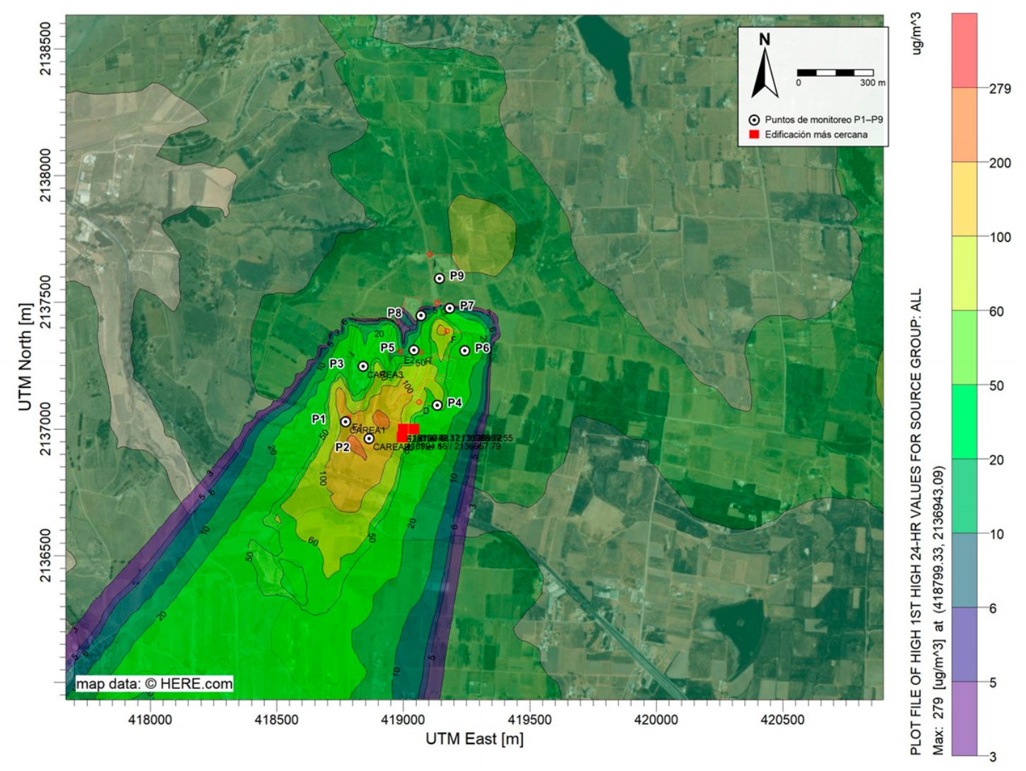
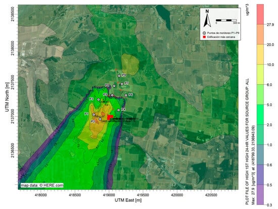
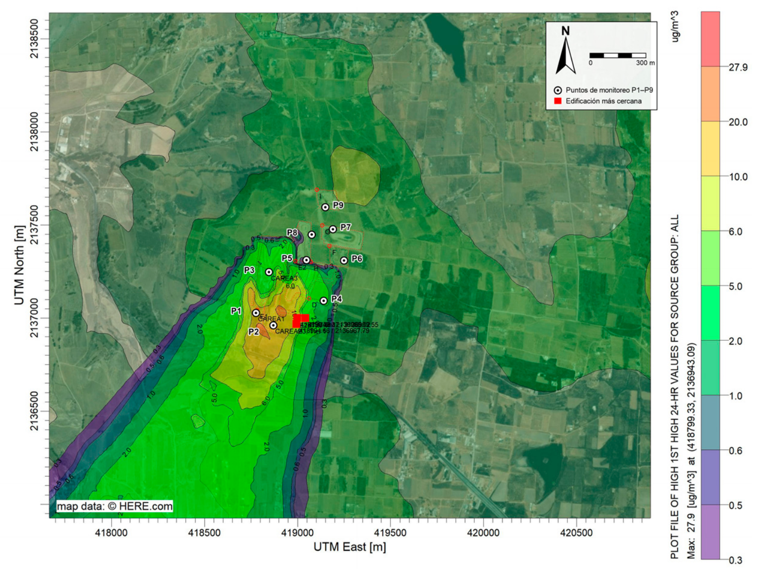
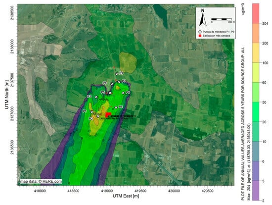
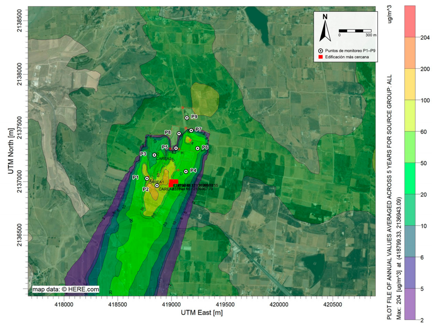
The input meteorology corresponds to the five years of hourly data (2021–2025) described in Section 3.1. With it, AERMOD calculated the concentration at each receptor for every hour of the period; from these, the 24 h averages of each day and the annual averages were obtained. The 24 h maps (Figure 4 and Figure 5) represent, at each receptor, the maximum 24 h concentration over the five years (first-highest value), i.e., the most unfavorable meteorological scenario of the period, appropriate for comparison with the 24 h limit values of NOM-025-SSA1-2021 and the WHO; the annual maps (Figure 6 and Figure 7) represent the five-year average and are representative of chronic exposure. Results were expressed in µg/m3 and presented as isopleth maps.
Figure 4.
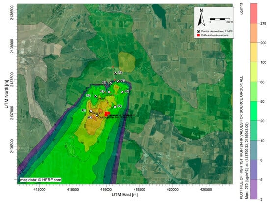
Distribution of the maximum 24 h PM10 concentration (first-highest value over the five years of meteorology, 2021–2025). Monitoring points P1–P9 and the nearest building (red box) are shown. The upper legend value (279 µg/m3) corresponds to the maximum concentration in the domain.
Figure 5.
Distribution of the maximum 24 h PM2.5 concentration (first-highest value over the five years of meteorology, 2021–2025). Monitoring points P1–P9 and the nearest building (red box) are shown. The upper legend value (27.9 µg/m3) corresponds to the maximum concentration in the domain.
Figure 6.
Distribution of the annual average PM10 concentration (average over the five years of meteorology, 2021–2025). Monitoring points P1–P9 and the nearest building (red box) are shown. The upper legend value (204 µg/m3) corresponds to the maximum concentration in the domain.
Figure 7.
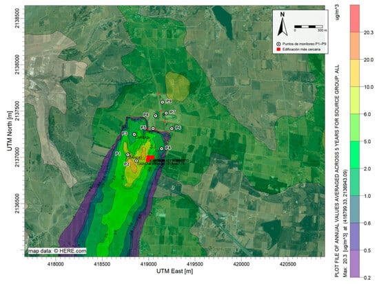
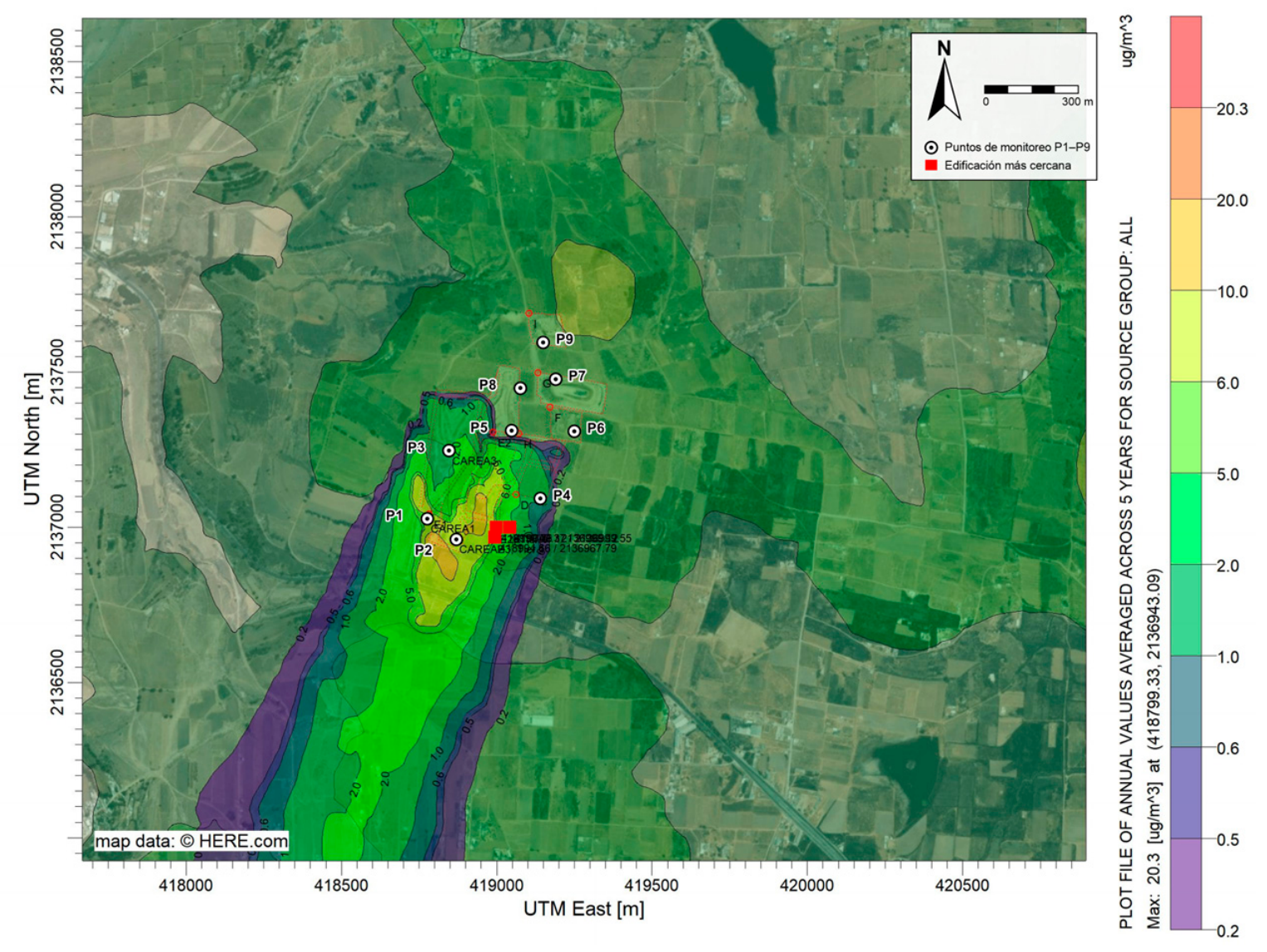
Distribution of the annual average PM2.5 concentration (average over the five years of meteorology, 2021–2025). Monitoring points P1–P9 and the nearest building (red box) are shown. The upper legend value (20.3 µg/m3) corresponds to the maximum concentration in the domain.
Calm hours (34.9% of the records) were processed with the standard AERMOD routine, which does not calculate concentrations for those hours and adjusts the divisor of the 24 h averages according to the US EPA calms policy [22]; since this treatment tends to underestimate concentrations under stagnant conditions, its effect is discussed in Section 4.7. The 500 m radius is the area of interest in the near field, where the monitoring points and the nearest building are located; the modeling domain (4.95 km × 4.95 km) covers the full extent of the plumes. The model results represent only the contribution of the IWC; the regional background concentration, estimated from the data of the nearest station of the Toluca Metropolitan Area (103 µg/m3 of PM10 and 97 µg/m3 of PM2.5 in 2025), is not part of the model output and was considered in the comparison with the measurements (Section 4.7). Finally, since the run does not include deposition or chemical transformation, the concentration at each receptor is the sum of the source contributions, each proportional to its emission rate. This linearity was used to: (i) identify the dominant source at the maximum-concentration receptor from the PM2.5/PM10 ratio of road emissions (0.1), which differs from that of the other sources; and (ii) evaluate the relative sensitivity of the concentrations to the input variables of Equation (1) (Section 4.8).
3.5. Particle Monitoring and Comparative Analysis
For particulate matter monitoring, a network of three portable particle counters was installed, arranged in a configuration of three triangles (Figure 1), each triangle covering critical areas of interest: the entrance gatehouse (P1), the vermicomposting area (P2), the administrative and maintenance area (P3), the excavation zone (P4), the heavy-vehicle traffic roads (P5), the working face (P6), the remediated cell (P7), the pumping station (P8) and the cover-material storage area (P9). Sampling was carried out from January to December 2025, three days per week, with continuous measurements throughout the site operating shift. Table 3 presents the measured concentrations together with the range of the AERMOD maximum 24 h concentration isopleths at the location of each point. Since the former are operating-shift averages and the latter are five-year maximum 24 h values, and since the run included neither discrete receptors nor hourly output, the two sets of values are not comparable and were not used to evaluate model performance (Section 4.7).
Table 3.
Measured concentration (12 h operating-shift average) and range of the AERMOD maximum 24 h concentration isopleths at the location of each monitoring point.
The nine points were selected based on the following criteria: proximity to each source type identified in the emission inventory, permanent presence of workers, accessibility and equipment safety. Dust Particle Counter TC-8100 (ZQFEE, Dongguan, China) portable optical counters were used, which measure by laser light scattering in the 0.3–10 µm range and log data every 5 min; they were placed 1.5 m above ground level, a height representative of the workers’ breathing zone. Each sampling day covered the full operating shift (07:00–19:00 h); the three instruments rotated among the vertices of their triangle according to a predefined schedule, so that the samples at each point were distributed across different days of the week and seasons of the year. Before the campaign and every 2 months, the three instruments were co-located for 1 h to verify their agreement and were compared with the records of the nearest station (Toluca 76675); in addition, the cleaning and zero calibration indicated by the manufacturer were performed. For quality control, records with relative humidity above 85% were removed, a condition under which hygroscopic particle growth causes overestimation in optical sensors [17,18,19], as were records with power failures or outside the measurement range; sampling days with less than 75% valid data were discarded. For each point, the mean concentration over the sampling period was calculated (Table 4).
Table 4.
PM10 and PM2.5 concentrations measured at the IWC monitoring points during the 12 h operating shift (07:00–19:00 h), January to December 2025.
4. Results and Discussion
4.1. Meteorological Data
Figure 2a shows the wind rose of the Toluca station for the 2021–2025 period, the same meteorology used in AERMOD. The analysis of the frequency distribution by direction and speed shows that winds from the NNE–NE sector are the most frequent, with ≈30% of the hours, followed by those from the N sector, with ≈14%; the values on the concentric circles of Figure (6.04–30.2%) correspond to the frequency scale. This predominance of NNE–NE and N winds correlates directly with the direction of travel of the air pollutant plume, indicating that IWC emissions are preferentially transported toward the W and SW of the site, affecting the communities located in that direction.
Regarding the wind speed distribution, the frequency plot (Figure 2b) shows that calm conditions (speed < 0.5 m/s) account for 34.9% of all records, a substantial proportion that favors the accumulation of pollutants near the site owing to poor horizontal ventilation. The most frequent speeds under active wind conditions lie in the 0.50–2.10 m/s range, which groups 54.9% of the records, followed by the 2.10–3.60 m/s (2.4%) and 3.60–5.70 m/s (0.6%) ranges. No speeds above 5.70 m/s were recorded, indicating a regime of predominant light to moderate winds. This combination of low speeds and a high frequency of calms, together with the predominant transport toward the SW, has implications for particle dispersion.
4.2. Topography
The topography of the study area, represented by the contour lines in Figure 3, shows elevations of 2680 to 2900 m a.s.l. in the vicinity of the IWC. The contour lines are relatively dense in the E and SE sectors of the site, indicating steep slopes, whereas toward the W and NW the contours gradually spread apart, showing flatter terrain. The IWC is therefore located in a transition zone, where wind flows descend the slopes and favor pollutant transport, as confirmed by the wind rose, which shows a predominance of flows from the NE and N sectors. As for its setting, the IWC sits in a slight topographic depression surrounded by natural elevations that can act as physical barriers modifying the dispersion of the pollutant plume.
The closely spaced contour lines to the east and south of the IWC indicate the presence of slopes that can induce wind channeling effects, accelerating the flow and transporting particles toward the southwest, while the flatter areas to the west could favor particle accumulation owing to lower wind speeds and greater atmospheric stability. Buildings can also alter the wind flow at the local scale, generating turbulent wakes that modify the dispersion and deposition of particles in their vicinity, a phenomenon that should be considered when configuring the AERMOD receptor grid and interpreting the isoconcentration maps. In addition, Figure 3 shows the proximity of buildings and human settlements in the SW sector of the IWC, at an approximate distance of 10 m from the nearest building, identified as point structures in the satellite image [22,29].
4.3. Operation Data
Table 1 presents the average data obtained during the monitoring year, which reflects the typical operating conditions of the site. Regarding the physicochemical characteristics of the MSW and soil, the physical composition of the by-products was grouped into organic waste (25%), inorganic waste (71%) and fines (4%); since the latter contribute to particulate matter, a soil textural composition of 63% sand, 36% silt and 1% clay was determined (it should be noted that textural silt, 2 to 50 µm, does not correspond to the AP-42 silt content, the <75 µm fraction obtained by sieving, which was 0.98% and is the value used in Equation (1)), with a soil moisture content of 1.05% (wet basis). The MSW, in turn, had an average moisture content of 11.09% (wet basis), a determining factor for estimating resuspension and material handling emissions.
4.4. Estimation of Particle Emissions
Based on the emission factors estimated with the AP-42 methodology [4] and the activity data collected during the monitoring year (Table 1), PM10 and PM2.5 emission rates were calculated for each of the sources identified at the Zinacantepec IWC. Table 2 presents the results for the main site activities, for which a release height of 0 m (ground-level emission) was used for all area sources. It should be noted that the control points (P1–P9) were not modeled as point sources: they are used only to identify the area source in which each monitoring point is located. The emission of each activity, calculated with Equations (1)–(6), was divided by the area of the corresponding polygon (Equation (7)) and distributed uniformly over it. Thus, the internal roads (along which P1, P2, P3, P5 and P8 are located) were represented by two polygons with a total area of 43,686 m2, the excavation zone (P4) by a 9504 m2 polygon, the working face (P6) by a 9720 m2 polygon, the remediated cell (P7) by a 21,265 m2 polygon and the cover-material area (P9) by a 10,671 m2 polygon (Table 2). PM2.5 emission rates were calculated independently for each source and modeled in a separate AERMOD run. For the roads, the PM2.5 rate is 10% of the PM10 rate, according to the ratio of the AP-42 particle size multipliers for industrial unpaved roads (0.15/1.5 lb/VMT) [4]. Since, in the absence of deposition, concentration is proportional to the emission rate and the roads are the dominant source at the maximum-concentration receptor, the ratio between the maximum modeled PM2.5 and PM10 concentrations is also 0.10. As shown, at control points P1, P2, P3, P5 and P8, vehicle resuspension was the most important source of PM2.5, resulting from the intense heavy-vehicle traffic and the extensive network of unpaved roads within the site. In the model, the excavation (P4) was entered without PM2.5 emissions, whereas the cover-material borrow area (P9) emits both fractions; this assignment is one of the causes of the PM2.5 underestimation discussed in Section 4.7. That the roads are the main source of particulate matter is consistent with the literature. The European Environment Agency sets emission factors for category 5.A “Solid waste disposal on land”, with values of 0.219 g/Mg for PM10 and 0.033 g/Mg for PM2.5 in mineral waste handling operations [37]. Finally, the remediated cell, a closed and covered area, showed PM10 emissions from wind erosion (1.0 × 10⁻⁶ g/(s·m2)); the PM2.5 emission of this source was not estimated, although AP-42 indicates a PM2.5/PM10 ratio of 0.15 for wind erosion [4]. On the other hand, the negligible emission from the working face, attributable to the moisture content of the MSW (Section 3.3), agrees with previous research showing the suppressive effect of moisture content on fugitive dust emissions [38].
4.5. Results of PM10 and PM2.5 Dispersion Modeling
Table 5 presents the PM10 and PM2.5 concentrations obtained with AERMOD. For PM10, the maximum 24 h concentration was 279.19 µg/m3 and the annual concentration 203.63 µg/m3, and for PM2.5, 27.92 µg/m3 and 20.26 µg/m3, respectively. The limit values of NOM-025-SSA1-2021 and the WHO guideline values [8,10] are included in Table 5 for reference only: because operational emissions were simulated over 24 h, the inventory omits sources and the model output does not include the background concentration (Section 3.4), these values are not used to assess regulatory compliance.
Table 5.
Maximum PM10 and PM2.5 concentrations in the modeling domain (24 h maximum and annual average) obtained with AERMOD.
Figure 4 shows the distribution of the maximum 24 h PM10 concentration. The highest values are located over the unpaved access road, next to P1 and P2; along the remaining internal roads (P3, P5 and P8), concentrations are lower, and a secondary local maximum appears over the remediated cell owing to wind erosion, consistent with the sources with the highest emission rate per unit area in Table 2 [20,25]. The prevailing NNE–NE winds (Figure 2a) transport the plume toward the SW, beyond the IWC perimeter and in the direction of the nearest building (red box). Since the mass emitted by the operational sources is overestimated and the inventory and the model output do not include all sources or the background concentration (Section 3.4), the map describes the orientation and shape of the plume but does not allow the extent of the zones where standards are exceeded, or the concentration at the building, to be established.
Figure 5 shows the maximum 24 h PM2.5 concentration. The highest values are located over the internal roads (Figure 1), which are the only relevant source of PM2.5 in the model [39,40]. The plume moves toward the SW, with the same orientation as the PM10 plume. As discussed in Section 4.7, the inventory does not include the PM2.5 sources of excavation, the working face and the remediated cell, or exhaust emissions, so the map does not represent the distribution of the fine fraction in those areas.
Figure 6 shows the annual average PM10 concentration, with the maximum in the vicinity of the sources (203.63 µg/m3). The annual plume is more compact than the 24 h plume and has the same SW orientation, indicating that the highest chronic exposure is concentrated within the IWC and along its SW boundary [41,42].
Figure 7 shows the annual average PM2.5 concentration. The maximum (20.26 µg/m3) is located over the unpaved access road, in the SW sector of the IWC (418799, 2136943; Figure 1). In line with the input meteorology described in Section 3.4, the prevailing NNE–NE winds transport the plume toward the SW, and concentrations decrease rapidly with distance from the roads [8].
Since the fine fraction has a longer atmospheric residence time than PM10, the plume orientation indicates that the agricultural land located SW of the IWC is the area in which an effect on air quality and on fine-particle deposition could be expected; its magnitude should be quantified with a corrected run.
4.6. Particle Monitoring
Table 4 presents the results of the air quality monitoring carried out at nine strategic points within the Zinacantepec IWC, corresponding to the average PM10 and PM2.5 concentrations during the 12 h operating shift over the sampling year. The recorded values reveal differences among the zones evaluated, reflecting the intensity of the operating activities closest to each area and their contribution to particulate matter generation. For PM10, the highest concentrations were observed at P4 and P6, followed by P5, P1, P2, P3 and P7, showing that earthmoving, waste unloading and compaction, and resuspension from vehicle traffic on unpaved roads are the main sources of PM10 within the site. In contrast, the lowest concentrations were recorded at P8 and P9, areas with lower operating activity or with characteristics that limit particle generation.
For PM2.5, the observed pattern is similar, although with markedly lower values than for PM10, which is consistent with the smaller particle size and its different behavior in the atmosphere. The highest concentrations were recorded at P6 and P4, followed by P1 and P7. These values indicate that the same sources that generate PM10 also contribute substantially to fine particle emissions, albeit to a lesser extent, since the fine fraction represents a smaller proportion of total fugitive dust emissions. The zone with the lowest PM2.5 concentration was P9, followed by P8, suggesting that these areas have a smaller impact on local air quality.
The operating-shift averages exceed the 24 h reference values of NOM-025-SSA1-2021 and the WHO at all points. This comparison is only indicative, since those values refer to 24 h averages and to the exposure of the general population, whereas the measurements correspond to 12 h within a workplace [43]; the assessment of occupational exposure is presented in Section 4.8. The excavation zone (P4) stands out as the critical point for both particle fractions, probably owing to the high intensity of earthmoving and the exposure of unwetted surfaces. Similarly, P6 shows high values due to daily waste handling, while the vehicle traffic road shows the impact of resuspension caused by heavy traffic at P1, P2, P3, P5 and P8.
The Lockwood landfill reported controlled annual emissions of 309.73 tons of PM10 and 30.97 tons of PM2.5 from unpaved roads, using AP-42 Section 13.2.2 emission factors, which underlines the magnitude of vehicle resuspension emissions [44]. In Medan, Indonesia, a study reported daily PM10 concentrations of 46.84 to 184.2 µg/m3 and PM2.5 concentrations of 38.94 to 163.1 µg/m3 at the Terjun dumpsite, with the highest concentrations in the active zone of the site. The same study found a strong relationship between air quality and the prevalence of acute respiratory infections in nearby communities, underlining the health impact of these emissions [45]. At the Pirana dumpsite in Ahmedabad, India, a 2024 study recorded daily concentrations of 200 µg/m3 for PM10 and 60 µg/m3 for PM2.5, both above the limits recommended by the WHO [46]. These values are close to those found at Zinacantepec, although the PM2.5 concentration at this site was higher, which could indicate differences in operating activities. This finding supports the site results, where the highest concentrations were associated with P4 and P6, areas of high operating intensity.
4.7. Comparative Assessment
Field monitoring was carried out exclusively during the 12 h operating shift in the IWC, so the values in Table 4 are 12 h rather than 24 h averages; consequently, their comparison with the 24 h limit values should be interpreted with caution. The AERMOD run did not include discrete receptors at the monitoring points or hourly output, so it was not possible to obtain modeled concentrations averaged over the same hours and days as the measurements or to calculate statistical performance indicators with paired values, such as FB, NMSE and FAC2 [47]. In addition, operational emissions were simulated over 24 h, although their rate was calculated for 12 h of operation (Section 3.4), so the simulated daily mass is twice that of the inventory. For these reasons, Table 3, which presents the measurements together with the isopleth range of the maximum 24 h concentration map at each point, does not allow model performance to be evaluated or the model to be said to reproduce the measurements at any point.
The only observation that does not depend on these differences is one of order of magnitude: at all points, the measured PM2.5 (109.43–200.61 µg/m3) is far higher than the isopleth range at its location (<0.3–20.0 µg/m3). A difference in this magnitude cannot be attributed to the different averaging periods and points to fine-particle sources that the inventory does not represent.
The PM2.5 underestimation suggests that the emission factors used do not adequately reflect fine particle generation in IWC operations. Notably, the measured PM2.5/PM10 ratio (0.69–0.94) is considerably higher than that implied by the AP-42 particle size multipliers for mechanically generated fugitive dust (≈0.10–0.15 in Sections 13.2.2 and 13.2.4) [4]. This difference may be due to fine particle sources not included in the inventory (e.g., exhaust emissions from diesel vehicles and machinery) and to the fact that optical particle counters can overestimate the fine fraction under high relative humidity or in the presence of mineral dust [17,18,19]. In any case, the difference between the measured values (often above 100 µg/m3) and the modeled values (below 30 µg/m3) indicates that the risk associated with PM2.5 could be underestimated if the assessment were based solely on the model.
The largest discrepancies were observed at P5–P9, away from the access road, where the modeled PM2.5 is below 0.6 µg/m3 compared with 109.43–200.61 µg/m3 measured. In the model, the excavation (D) and the remediated cell (G) do not emit PM2.5, the working face (F) emits neither fraction and the cover-material borrow area (I) has a very low emission (Table 2), so the modeled PM2.5 at those points comes almost exclusively from the roads; the PM2.5 sources of these areas and the exhaust emissions from machinery are not represented. Moreover, the regional background concentration is not part of the model output, and the high frequency of calms (34.9%), hours for which AERMOD does not calculate concentrations, favors underestimation under stagnant conditions [48,49].
AERMOD, by using AP-42 emission factors based on studies conducted in other contexts, may not fully reflect the high PM2.5 generation associated with the specific operations of the Zinacantepec IWC, such as the compaction of waste with a high organic content (11.09% moisture), the resuspension of fine waste at P6, earthmoving or the resuspension of fine particles by heavy-vehicle traffic on the roads. Likewise, the high frequency of calms (34.9%) and the occurrence of thermal inversions in the Toluca Valley can generate fine-particle accumulation conditions that the model, in its standard configuration, does not reproduce accurately owing to its limitations in simulating low-wind conditions, particularly the absence of plume meander treatment for area sources [50].
This comparison reinforces the need to complement modeling with intensive monitoring campaigns that capture the spatial and temporal variability of concentrations. The model provides an overview of dispersion and allows the plume orientation and critical areas to be identified, while monitoring provides empirical data that reflect the actual conditions of the site. Integrating both approaches—modeling and monitoring—strengthens air quality assessment [51], provided that the modeling represents the actual operating schedule and a complete inventory and that the comparison is made with values matched in time and space.
4.8. Implications
The application of AERMOD provides information that point monitoring within the IWC cannot offer, although in this study it can be used only in spatial and relative terms. First, it shows that the plumes are oriented toward the SW, beyond the site perimeter and in the direction of the nearest building and the agricultural land, which indicates where off-site monitoring and control measures should be prioritized. Second, it allows the dominant source to be identified: since the concentration is the sum of contributions proportional to the emission of each source (Section 3.4) and the PM2.5/PM10 ratio of road emissions (0.1) differs from that of the other sources (0 for the excavation and the remediated cell), the contribution of the roads to PM10 equals 10 times the modeled PM2.5; at the maximum-concentration receptor, the roads are practically the only modeled source. Third, the concentration is directly proportional to road emissions, so a ±20% variation in vehicle-kilometers traveled, silt content or fleet weight changes the concentration by ±20%, +17.8/−18.2% and +8.6/−9.6%, respectively (Equation (1), with a = 0.9 and b = 0.45), whereas the moisture content, which only affects the material handling sources, has an effect of less than 1%. In contrast, absolute concentrations, the extent of the zones where standards are exceeded and the emission reductions required to meet them require repeating the run with a 12 h hourly emission profile, an inventory that includes exhaust emissions and traffic on the working face, and the background concentration; they are therefore not quantified in this study.
Regarding health implications, it is necessary to distinguish between ambient air quality, worker exposure and health effects. The reference values of NOM-025-SSA1-2021 and the WHO [8,10] protect the general population and refer to 24 h and annual averages; they are therefore applicable only to off-site receptors, where concentrations were estimated with the model and not measured. For workers, the applicable framework is NOM-010-STPS-2014, which sets time-weighted average exposure limit values of 2.5 mg/m3 for the respirable fraction and 10 mg/m3 for the inhalable fraction of particles not otherwise specified [52]. The 8 h time-weighted average concentration estimated from the 12 h shift measurements (338 µg/m3, i.e., 0.34 mg/m3 of PM10 at the most exposed point, P4, considering a 12 h shift) is below these values; nevertheless, it far exceeds the WHO guideline values, which are based on health effects documented even at low concentrations, so the daily and prolonged exposure of workers during 12 h shifts constitutes a risk that should be reduced [41,53]. Since no concentrations were measured beyond the site perimeter and no health indicators were assessed, the results of this study identify zones with high concentrations but do not allow the exposure of nearby communities to be quantified or effects on their health to be demonstrated.
Based on these results, the priority measure is dust control on the internal roads, the dominant source in the inventory and in the model, and, since the highest measured concentrations were recorded at the excavation and the working face, also in these areas. The control efficiency required to meet the standards should be established with a corrected run; the efficiency of watering depends on its frequency and intensity [4], so its effectiveness should be verified through monitoring before and after implementation. Complementary measures are as follows. Source control measures include frequent watering of unpaved roads and active areas to reduce dust resuspension, paving the priority roads with the highest vehicle traffic, and reducing vehicle speeds within the site to limit fugitive dust generation.
Regarding personal protection, it is essential to provide workers with adequate personal protective equipment (PPE), in particular N95 or higher-grade respirators (such as N99 or P100), which offer a filtration efficiency of 95% or more for fine and ultrafine particles, and to ensure their training in the use and maintenance of this equipment [54,55]. Studies at final disposal sites have shown that the use of surgical or cloth masks, common among workers at this type of facility, is insufficient to protect them against the inhalation of fine particles and toxic compounds, so certified PPE must be provided [41]. In addition, it is suggested to install a continuous air quality monitoring system at strategic points within the landfill to warn of critical pollution episodes and trigger safety protocols, such as suspending activities or requiring higher-protection PPE under adverse conditions. These measures will not only help reduce worker exposure but will also help minimize the impact on communities located in the prevailing wind direction, improving the environmental and social sustainability of the site [20,43].
Finally, these results have implications for land-use planning. Impact assessments usually analyze each facility in isolation, although the plumes of nearby sources (other disposal sites, borrow pits, industries and roads) overlap over the same residential and commercial areas. AERMOD allows multiple sources and facilities within a radius of up to 50 km to be included in a single run and the background concentration to be added, so the approach presented here can be extended to a cumulative assessment if the emission inventories of the other sources are available; for transport over longer distances or in complex wind fields, Lagrangian (CALPUFF) or regional Eulerian (CMAQ) models are required [22,23]. In this context, maps such as those in Figure 4, Figure 5, Figure 6 and Figure 7, obtained with an hourly emission profile and a complete inventory, can be used to: (i) define buffer zones in which residential development is restricted; (ii) assess, before authorizing a new facility or the expansion of an existing one, whether its contribution, added to that of existing sources, would exceed the standards at sensitive receptors; and (iii) prioritize control measures and monitoring in the prevailing wind directions. For this information to effectively influence decisions, it is recommended that environmental authorities require cumulative modeling in the environmental impact statements of final disposal sites and neighboring facilities.
5. Conclusions
Using five years of meteorology (2021–2025), AERMOD indicates that the PM10 and PM2.5 plumes of the IWC are oriented toward the SW, beyond the site perimeter and in the direction of the nearest building, and that the highest concentrations are located over the unpaved access road. Because operational emissions were simulated over 24 h instead of the 12 h shift, the inventory omits relevant sources and the model output does not include the background concentration, the modeled values were not used to quantify concentrations or distances at which standards are exceeded.
The concentrations measured during the operating shift (PM10: 140.33–225.23 µg/m3; PM2.5: 109.43–200.61 µg/m3) exceed the WHO ambient air quality guideline values at all points, although they are below the occupational exposure limits of NOM-010-STPS-2014. PM2.5 concentrations should be confirmed with a reference method, given the possible bias of optical sensors.
According to the emission inventory and the source contributions estimated with AERMOD, the internal unpaved roads are the dominant source of PM10 at the maximum-concentration receptor. The measurements, however, show the highest concentrations at the excavation zone (P4) and the working face (P6), so emissions from these areas should be characterized in greater detail.
Measured concentrations exceed the WHO guideline values in the operational areas of the IWC. Dust control on the internal roads, together with measures at the excavation and the working face (reducing traffic speed, paving the most heavily trafficked sections and using certified respirators), is a priority; the control efficiency required to meet the standards should be established with a corrected run, and the effectiveness of the measures should be verified through continuous monitoring before and after implementation.
Author Contributions
Conceptualization, S.F.R., M.d.C.H.-B. and F.C.-R.; methodology, S.F.R., M.d.C.H.-B., A.L.G.d.C. and M.d.C.M.-S.; validation, S.F.R., A.L.G.d.C., F.C.-R., M.d.C.M.-S. and D.G.-L.; formal analysis, S.F.R., A.L.G.d.C., F.C.-R., M.d.C.M.-S. and D.G.-L.; investigation, S.F.R. and M.d.C.H.-B.; resources, S.F.R., M.d.C.H.-B., F.C.-R. and M.d.C.M.-S.; data curation, M.d.C.H.-B., F.C.-R., A.L.G.d.C. and D.G.-L.; writing—original draft preparation, S.F.R., M.d.C.H.-B., A.L.G.d.C. and M.d.C.M.-S.; writing—review and editing, S.F.R., M.d.C.H.-B., A.L.G.d.C., D.G.-L., F.C.-R. and M.d.C.M.-S.; supervision, M.d.C.H.-B. and F.C.-R.; project administration, F.C.-R. and M.d.C.M.-S. All authors have read and agreed to the published version of the manuscript.
Funding
This research received no external funding.
Data Availability Statement
The original PM10 and PM2.5 monitoring records are not available owing to the loss of the measurement instrument files. The average concentrations at each monitoring point are presented in Table 4.
Acknowledgments
The authors thank the company “Mantenimientos y Servicios Ambientales S.A. de C.V.” for the facilities provided for the in situ characterization of the disposed MSW. They also thank the Secretariat of Science, Humanities, Technology and Innovation (SECIHTI) for the scholarship granted to a doctoral student in Environmental Sciences at the Tecnológico Nacional de México/Instituto Tecnológico de Toluca, Graduate Studies and Research Division.
Conflicts of Interest
The authors declare no conflicts of interest.
Abbreviations
The following abbreviations are used in this manuscript:
| PM10 | Particulate matter < 10 micrometers |
| PM2.5 | Particulate matter < 2.5 micrometers |
| MSW | Municipal solid waste |
| WHO | World Health Organization |
| EPA | Environmental Protection Agency |
| IWC | Integrated Waste Center |
| C | Cell |
| P | Monitoring point |
| AC | Cell expansion |
| Cs | Remediated cell |
| INEGI | National Institute of Statistics and Geography |
| m | meter |
| h | hour |
| s | second |
| N | North |
| E | East |
| W | West |
| S | South |
| SW | Southwest |
| NE | Northeast |
| µg | Microgram |
| m3 | Cubic meter |
References
- Cook, E.; Ionkova, K.; Bhada-Tata, P.; Yadav, S.; van Woerden, F. What a Waste 3.0: Global Snapshot of Solid Waste Management Toward Circularity Until 2050; Urban Development Series; World Bank Group: Washington, DC, USA, 2026. [Google Scholar] [CrossRef] [Scilit]
- Kaza, S.; Yao, L.C.; Bhada-Tata, P.; Van Woerden, F.; Levine, D. What a Waste 2.0: A Global Snapshot of Solid Waste Management to 2050; The World Bank: Washington, DC, USA, 2018. [Google Scholar] [CrossRef] [Scilit]
- Bihałowicz, J.S.; Rogula-Kozłowska, W.; Krasuski, A. Contribution of landfill fires to air pollution—An assessment methodology. Waste Manag. 2021, 125, 182–191. [Google Scholar] [CrossRef] [Scilit] [PubMed]
- Compilation of Air Pollutant Emission Factors (AP-42), 5th ed.; U.S. Environmental Protection Agency: Research Triangle Park, NC, USA, 1995; Volume I. Available online: https://www.epa.gov/air-emissions-factors-and-quantification/ap-42-compilation-air-emissions-factors-stationary-sources (accessed on 26 July 2026).
- Zamorategui-Molina, A.; Álvarez Guzmán, G.; Esquivel Longoria, M.I.; Baltazar Vera, J.C.; Serafín Muñoz, A.H. Dispersion of PM2.5 particles emitted by the waste dump fire in the city of Guanajuato, Mexico. Asian J. Atmos. Environ. 2025, 19, 27. [Google Scholar] [CrossRef] [Scilit]
- Carter, W.; Feig, G.; De Vos, S. Quantifying the air quality benefits of a waste collection offsetting intervention in the Vaal Triangle Airshed Priority Area (VTAPA). Clean Air J. 2025, 35, 1–7. [Google Scholar] [CrossRef] [Scilit]
- Hamidah, F.J.; Ariska, D.O.; Asih, A.Y.P.; Muna, K.U.N.E.; Wikurendra, E.A.; Rangga, J.U. Impact of particulate matter exposure on forced vital capacity and respiratory symptoms in landfill worker. J. Air Pollut. Health 2025, 10, 341–362. [Google Scholar] [CrossRef] [Scilit]
- World Health Organization. Global Air Quality Guidelines 2021: Particulate Matter (PM2.5 and PM10), Ozone, Nitrogen Dioxide, Sulfur Dioxide and Carbon Monoxide. Available online: https://www.who.int/publications/i/item/9789240034228 (accessed on 21 July 2026).
- Stroh, E. Air Pollution in Europe and Children’s Health (Briefing and Factsheet). AirClim 2023. Available online: https://lup.lub.lu.se/search/files/146390559/air_pollution_in_europe_and_childrens_health.pdf (accessed on 21 July 2026).
- NOM-025-SSA1-2021; Salud Ambiental. Valores Límite Permisibles para la Concentración de Partículas Suspendidas PM10 y PM2.5 en el Aire Ambiente y Criterios para su Evaluación. Diario Oficial de la Federación: Mexico City, México, 2021. Available online: https://dof.gob.mx/nota_detalle.php?codigo=5633855&fecha=27/10/2021#gsc.tab=0 (accessed on 26 July 2026).
- Dávila-Samano, A.R.; Castillo-Suárez, L.A.; Linares-Hernández, I.; García-Colindres, M.A.; Martínez-Miranda, V. Efectos ambientales en el aire, agua y suelo de los residuos sólidos urbanos de un relleno sanitario del Estado de México [Environmental effects on air, water and soil of municipal solid waste from a sanitary landfill in the State of Mexico]. Investig. Cienc.-Univ. Autónoma Aguascalientes 2024, 91, 1–23. [Google Scholar] [CrossRef] [Scilit]
- NOM-017-STPS-2008; Equipo de Protección Personal-Selección, uso y Manejo en los Centros de Trabajo. Diario Oficial de la Federación: México City, México, 2008. Available online: https://www.dof.gob.mx/normasOficiales/3558/stps/stps.htm (accessed on 22 July 2026).
- NOM-030-STPS-2009; Servicios Preventivos de Seguridad y Salud en el Trabajo-Funciones y Actividades. Diario Oficial de la Federación: México City, México, 2009. Available online: https://sidof.segob.gob.mx/notas/docFuente/5125949 (accessed on 22 July 2026).
- Opara, A.; Akaolisa, C.; Akakuru, C.; Nkwoada, A.; Ibe, F.; Verla, A.; Chukwuemeka, I. Particulate matter exposure and non-cancerous inhalation health risk assessment of major dumpsites of Owerri metropolis, Nigeria. Environ. Anal. Health Toxicol. 2021, 36, e2021025. [Google Scholar] [CrossRef] [Scilit] [PubMed]
- Peter, A.; Nagendra, S. Dynamics of PM2.5 pollution in the victinity of the old municipal waste dumpsite. Environ. Monit. Assess. 2021, 193, 281. [Google Scholar] [CrossRef] [Scilit] [PubMed]
- Jawwad, M.A.S.; Adibhaskara, A.R.; Murti, R.H.A. Particulate matter dispersion patterns near Klotok landfill site. IOP Conf. Ser. Earth Environ. Sci. 2025, 1454, 012026. [Google Scholar] [CrossRef] [Scilit]
- Atfeh, B.; Barcza, Z.; Groma, V.; Tordai, Á.V.; Mészáros, R. Performance Assessment of Low- and Medium-Cost PM2.5 Sensors in Real-World Conditions in Central Europe. Atmosphere 2025, 16, 796. [Google Scholar] [CrossRef] [Scilit]
- Badura, M.; Batog, P.; Drzeniecka-Osiadacz, A.; Modzel, P. Evaluation of Low-Cost Sensors for Ambient PM2.5 Monitoring. J. Sens. 2018, 2018, 5096540. [Google Scholar] [CrossRef] [Scilit]
- Lee, H.; Kang, J.; Kim, S.; Im, Y.; Yoo, S.; Lee, D. Long-Term Evaluation and Calibration of Low-Cost Particulate Matter (PM) Sensor. Sensors 2020, 20, 3617. [Google Scholar] [CrossRef] [Scilit] [PubMed]
- Abidin, A.; Maziya, F.; Susetyo, S.; Yoneda, M.; Matsui, Y. Exposure particulate matter (PM2.5) and health risk assessment on informal workers in landfill site, Indonesia. Environ. Chall. 2023, 13, 100795. [Google Scholar] [CrossRef] [Scilit]
- Kermani, M.; Farzadkia, M.; Kalantari, R.R.; Bahmani, Z. Fine particulate matter (PM2.5) in a compost facility: Heavy metal contaminations and health risk assessment, Tehran, Iran. Environ. Sci. Pollut. Res. 2018, 25, 15715–15725. [Google Scholar] [CrossRef] [Scilit] [PubMed]
- U.S. Environmental Protection Agency. AERMOD Model Formulation and Evaluation; EPA-454/R-20-001; U.S. Environmental Protection Agency: Washington, DC, USA, 2006. Available online: https://www.epa.gov/scram/air-quality-dispersion-modeling-preferred-and-recommended-models (accessed on 22 July 2026).
- Air Quality Monitoring and Data Analysis. Available online: https://www.epa.gov/air-quality-analysis (accessed on 22 July 2026).
- Popoola, A.O.; Jimoda, L.A.; Olu-Arotiowa, O.A.; Ogunkunle, O.; Laseinde, O.T.; Adebanjo, S.A.; Raji, W.A. Dispersion of PM and VOC pollutants from open burning of municipal solid wastes on host communities: Emission inventory estimation and dispersion modelling study. Environ. Sci. Atmos. 2023, 3, 1090–1109. [Google Scholar] [CrossRef] [Scilit]
- Ramadan, B.S.; Budihardjo, M.A.; Syafrudin; Huboyo, H.S.; Sari, S.A. Analysis of particulate matter (PM10 and PM2.5) emissions from Jatibarang landfill: Implications for air quality and health. IOP Conf. Ser. Environ. Earth Sci. 2025, 1477, 012033. [Google Scholar] [CrossRef] [Scilit]
- Gobierno del Estado de México. Portal de Consulta del Sistema Integral de Residuos del Estado de México. Available online: http://187.188.85.202:8095/consulta-sirem/ (accessed on 24 July 2026).
- NOM-083-SEMARNAT-2003; Especificaciones de Protección Ambiental para la Selección del sitio, Diseño, Construcción, Operación, Monitoreo, Clausura y Obras Complementarias de un sitio de Disposición Final de Residuos Sólidos Urbanos y de Manejo Especial. Diario Oficial de la Federación (DOF): México City, México, 2003. Available online: https://dof.gob.mx/nota_detalle.php?codigo=658648&fecha=20/10/2004#gsc.tab=0 (accessed on 24 July 2026).
- NTEA-020-SeMAGEM-RS-2019; Establece los Requisitos Para la Instalación y Operación de los Centros Integrales de Residuos en el Estado de México. Gobierno del Estado de México: Toluca, México, 2019. Available online: http://legismex.mty.itesm.mx/estados/ley-edm/EM-NT-NTEA-020-SEMAGEM-RS-2019.pdf (accessed on 24 July 2026).
- Instituto Nacional de Geografía e Informática. Mapa Digital V.6.3.0. Instituto Nacional de Estadística y Geografía. Available online: https://gaia.inegi.org.mx/mdm6/?v=bGF0OjE5LjI0OTUwLGxvbjotOTkuODc5NDksejoxMCxsOmMxMTFzZXJ2aWNpb3N8dDExMXNlcnZpY2lvc3xjcnN1X3NpdGlvX2Rpc3Bvc2ljaW9u (accessed on 24 July 2026).
- Hernández-Contreras, G.I.; Díaz-Archundia, L.V.; Szanto-Narea, M.; Mañon-Salas, M.C.; Hernández-Berriel, M.C.; Cuellar-Robles, F. Methodological Proposal for the “In Situ” Characterization of Municipal Solid Waste After Final Disposal. Recycling 2026, 11, 131. [Google Scholar] [CrossRef] [Scilit]
- NMX-AA-022-1985; Protección al Ambiente-Contaminación del Suelo Residuos Sólidos Municipales-Selección y Cuantificación de Subproductos. Secretaría de Economía: Ciudad de México, México, 1985. Available online: http://legismex.mty.itesm.mx/normas/aa/aa022.pdf (accessed on 24 July 2026).
- NMX-AA-132-SCFI-2016; Muestreo de Suelos Para la Identificación y la Cuantificación de Metales y Metaloides, y Manejo de la Muestra. Diario Oficial de la Federación (DOF): Ciudad de México, México, 2016. Available online: http://www.economia-nmx.gob.mx/normas/nmx/2010/nmx-aa-132-scfi-2016.pdf (accessed on 24 July 2026).
- Food and Agriculture Organization of the United Nations (FAO). Guía para la Descripción de Suelos, 4th ed. (Spanish version); FAO: Rome, Italy, 2009; Available online: https://openknowledge.fao.org/server/api/core/bitstreams/b54d0348-dfce-413c-bd5d-142b3a14a049/content (accessed on 24 July 2026).
- NMX-AA-015-1985; Protección al Ambiente—Contaminación del Suelo—Residuos Sólidos Municipales—Muestreo—Método de Cuarteo. Secretaria de Comercio y Fomento Industrial: Ciudad de México, México, 1985. Available online: https://biblioteca.semarnat.gob.mx/janium/Documentos/Ciga/agenda/DOFsr/NMX-AA-015-1985.pdf (accessed on 24 July 2026).
- NMX-AA-016-1984; Protección al Ambiente-Contaminación del Suelo-Residuos Sólidos Municipales-Determinación de Humedad. Secretaría de Economía: Ciudad de México, México, 1985. Available online: https://biblioteca.semarnat.gob.mx/janium/Documentos/Ciga/agenda/DOFsr/NMX-AA-016-1984.pdf (accessed on 26 July 2026).
- NMX-AA-018-1984; Protección al Ambiente-Contaminación de Suelo Residuos Sólidos Municipales-Determinación de Cenizas. Secretaría de Economía: Ciudad de México, México, 1984. Available online: https://biblioteca.semarnat.gob.mx/janium/Documentos/Ciga/agenda/DOFsr/NMX-AA-018-1984.pdf (accessed on 27 July 2026).
- EMEP/EEA Air Pollutant Emission Inventory Guidebook 2023: 5.A Solid Waste Disposal on Land. Available online: https://www.eea.europa.eu/publications/emep-eea-guidebook-2023 (accessed on 26 July 2026).
- Traven, L.; Linšak, Ž.; Crvelin, G. Mitigating landfill gas emissions: The effectiveness of HDPE covers in reducing atmospheric concentrations of H2S, NH3, and PM10. Arh. Hig. Rada Toksikol. 2024, 75, 259–269. [Google Scholar] [CrossRef] [Scilit] [PubMed]
- Arya, R.; Ahlawat, S.; Yadav, L.; Jangirh, R.; Mondal, A.; Sharma, S.; Gurjar, B.; Nemitz, E.; Mandal, T. Particle Size Distribution from Municipal Solid Waste Burning Over National Capital Territory, India. Environ. Sci. Proc. 2022, 19, 26. [Google Scholar] [CrossRef] [Scilit]
- Méndez, J.; Pinto, L.; Galvis, B.; Pachón, J. Estimation of resuspended dust emission factors before, during and after road paving process in Bogota. Cienc. Ing. Neogranadina 2017, 27, 43–60. [Google Scholar] [CrossRef] [Scilit]
- Senthilnathan, R. Occupational exposure to size-segregated particulate matter in solid waste handling: A Multi-analytical and Dosimetric study. Environ. Prot. Eng. 2026, 52, 45–63. [Google Scholar] [CrossRef] [Scilit]
- Giosanu, D.; Marian, M.; Zaharia, A. The influence of meteorological topographical parameters on the dispersion of PM10 and CO pollutants. Curr. Trends Nat. Sci. 2021, 10, 92–98. [Google Scholar] [CrossRef] [Scilit]
- Kwarteng, L.; Devasurendra, A.M.; Laskaris, Z.; Arko-Mensah, J.; Amoabeng Nti, A.A.; Takyi, S.; Acquah, A.A.; Dwomoh, D.; Basu, N.; Robins, T.; et al. Occupational exposures to particulate matter and PM2.5-associated polycyc lic aromatic hydrocarbons at the Agbogbloshie waste recycling site in Ghana. Environ. Int. 2022, 158, 106971. [Google Scholar] [CrossRef] [Scilit] [PubMed]
- Washoe County. Lockwood Landfill Technical Support Document. Available online: https://washoe-nv.legistar.com/Calendar.aspx (accessed on 27 July 2026).
- Intan, T.K.; Munir, D.; Soeroso, N.N.; Ichwan, M.; Khair, H.; Suryati, I. The relevancy-analysis of air quality index to Acute Respiratory Infection (ARI) in a landfill site of Medan. IOP Conf. Ser. Environ. Earth Sci. 2023, 1241, 012117. [Google Scholar] [CrossRef] [Scilit]
- D’Costa, J.; Keita, D.S.; Braganza, V.J.; Patel, H. Environmental Impact Assessment of the Solid Waste Landfill in Ahmedabad. J. Inst. Eng. India Ser. A. 2024, 105, 589–601. [Google Scholar] [CrossRef] [Scilit]
- Chang, J.C.; Hanna, S.R. Air quality model performance evaluation. Meteorol. Atmos. Phys. 2004, 87, 167–196. [Google Scholar] [CrossRef] [Scilit]
- Askariyeh, M.H.; Kota, S.H.; Vallamsundar, S.; Zietsman, J.; Ying, Q. AERMOD for near-road pollutant dispersion: Evaluation of model performance with different emission source representations and low wind options. Transp. Res. D Transp. Environ. 2017, 57, 392–402. [Google Scholar] [CrossRef] [Scilit]
- Srivastava, A.; Kumar, A.; Elumalai, S. Evaluating Dispersion Modeling of Inhalable Particulates (PM10) Emissions in Complex Terrain of Coal Mines. Environ. Model 2021, 26, 385–403. [Google Scholar] [CrossRef] [Scilit]
- Venkatram, A.; Pandey, G.; Arunachalam, S. Incorporating meander to account for the impact of low winds in area source modeling; AERMOD as a case study. J. Air Waste Manag. Assoc. 2025, 75, 27–36. [Google Scholar] [CrossRef] [Scilit] [PubMed]
- Kumar, A.; Dikshit, A.K.; Patil, R.S. Use of simulated and observed meteorology for air quality modeling and source ranking for an industrial region. Sustainability 2021, 13, 4276. [Google Scholar] [CrossRef] [Scilit]
- NOM-010-STPS-2014; Agentes Químicos Contaminantes del Ambiente Laboral-Reconocimiento, Evaluación y Control. Diario Oficial de la Federación: Mexico City, Mexico, 2014. Available online: https://dof.gob.mx/normasOficiales/5359/stps2a11_C/stps2a11_C.html (accessed on 30 October 2026).
- Schraufnagel, D.E.; Balmes, J.R.; Cowl, C.T.; De Matteis, S.; Jung, S.H.; Mortimer, K.; Perez-Padilla, R.; Rice, M.B.; Riojas-Rodriguez, H.; Sood, A.; et al. Air pollution and noncommunicable diseases: A review by the Forum of International Respiratory Societies’ Environmental Committee, Part 1: The damaging effects of air pollution. Chest 2019, 155, 409–416. [Google Scholar] [CrossRef] [Scilit] [PubMed]
- 29 CFR 1910.134; Respiratory Protection Standard. U.S. Department of Labor: Washington, DC, USA, 1998. Available online: https://www.osha.gov/laws-regs/regulations/standardnumber/1910/1910.134 (accessed on 27 July 2026).
- National Institute for Occupational Safety and Health. Respiratory Protective Devices: Certification and Standards. Centers for Disease Control and Prevention. Available online: https://www.cdc.gov/niosh/ (accessed on 27 July 2026).

Disclaimer/Publisher’s Note: The statements, opinions and data contained in all publications are solely those of the individual author(s) and contributor(s) and not of MDPI and/or the editor(s). MDPI and/or the editor(s) disclaim responsibility for any injury to people or property resulting from any ideas, methods, instructions or products referred to in the content. |
© 2026 by the authors. Licensee MDPI, Basel, Switzerland. This article is an open access article distributed under the terms and conditions of the Creative Commons Attribution (CC BY) license.