


Abstract
Coal handling port terminals are a recognized source of particulate matter (PM) in tropical coastal settings, where the exposure of nearby communities is a growing environmental justice concern. This study describes the spatial distribution of PM10 and PM2.5 and evaluates the exposure of a Zenú Indigenous community in the Gulf of Morrosquillo (Santiago de Tolú, Sucre, Colombia), in the area of influence of a coal export terminal, under a monitoring program mandated by Constitutional Court Ruling T-433 of 2023. A receptor–reference design (two exposed receptor stations and one reference station) was sampled over a rainy and dry season campaign in 2024 (105 valid daily records) and read together with an emission inventory, an AERMOD/WRF dispersion model run for six production scenarios, the terminal’s operational record and an environmental sanctioning file. No daily value exceeded the national 24 h limits (Resolution 2254 of 2017); all station days fell in the “Good” band of the national Air Quality Index except one PM2.5 day at the reference station (18.96 µg m−3, “Acceptable”) that coincided with a field-logged biomass burning episode, and the ratio of campaign mean PM2.5 to PM10 (0.29–0.42) indicates a coarse-dominated mass. In the dispersion model, the terminal source increment alone does not exceed the 24 h or annual limits at any community receptor or monitoring point in any scenario; this refers to the modelled increment, not to total ambient concentrations. A model-based screening comparison (not a source apportionment) between the modelled terminal maximum and the measured maximum 24 h PM10 at the monitoring points gave ratios of 41–118%, with values above 100% where the maximum modelled over two meteorological years exceeds the maximum measured in a short campaign, the two maxima being unpaired in time, and the environmental authority documented coal piles exceeding containment barriers. We argue that compliant results should not be read on their own, as evidence of no impact, because mass concentration standards do not register composition, deposition or source contributions below the threshold. Implications for the Prior Consultation process are discussed, together with the complementary metrics that would constrain the port contribution observationally (quantitative dustfall monitoring, identified as a priority, and elemental/black carbon speciation). Finally, deep learning architectures were employed to predict PM10 and PM2.5 concentrations, achieving RMSE values ranging from 0.36 µg/m3 during the dry season to 0.002 µg/m3 during the wet season for PM10, and from 0.03 µg/m3 during the dry season to 0.0007 µg/m3 during the wet season for PM2.5 during the training stage, as exploratory DL model is presented in this research.
1. Introduction
1.1. Particulate Matter in Coastal Settings Influenced by Coal Ports
Airborne particulate matter (PM) is one of the environmental risk factors most consistently associated with adverse human health outcomes, and the World Health Organization (WHO) treats it as a public health problem of global scale [1,2]. The health burden of PM is size-dependent: the fine fraction (PM2.5) penetrates deeper into the respiratory tract and reaches the alveolar region, so it carries greater sanitary relevance than the coarse fraction (PM2.5–10), which is largely deposited in the upper airways [3,4]. Short- and long-term exposure to PM2.5 has been linked to increased respiratory and cardiovascular morbidity and mortality across a wide range of settings and concentrations [4,5,6,7].
Coal handling port terminals are a well-documented source of PM in coastal and tropical environments. The unloading, stacking, reclaiming and shiploading of coal, together with wind erosion of open stockpiles and the movement of heavy vehicles on unpaved surfaces, release both coarse and fine particles enriched in carbonaceous material [8,9]. Recent community monitoring next to a coal export terminal showed higher PM and black carbon when the monitors were downwind of the terminal and during visible stockpile handling [10]. In the Colombian Caribbean, where a large share of the national coal output is exported, studies along the Cesar–La Guajira–Magdalena mining and transport corridor have reported measurable respiratory effects in communities living near coal railways and terminals, even where ambient concentrations remain moderate [11,12,13]. The atmospheric particularities of the Gulf of Morrosquillo—an open, low-relief coastline swept by the trade winds and a diurnal sea breeze and periodically reached by long-range Saharan dust intrusions—strongly modulate the local transport, dilution and composition of PM [14,15,16].
1.2. From a Temporal to a Spatial and Exposure-Oriented Reading
Community-scale monitoring program typically record meteorology at station visits. In such programs, the seasonal (rainy vs. dry) contrast integrates emission, transport and removal processes in a single signal, so the spatial gradient between stations and the relative weight of the fine fraction are more informative than the temporal contrast for the specific question of community exposure [17,18,19]. This study therefore adopts a receptor–reference design (two exposed receptor stations plus one reference station) as a pragmatic instrument to size the exposure of the community and to compare it against health-based thresholds, treating season as a modulating covariate.
This reframing also exposes a deeper question that motivates the present work. Regulatory air quality standards are written as mass concentration limits averaged over fixed windows: a station “complies” when its 24 h gravimetric mass stays below a numerical threshold, irrespective of what the mass is made of or where it settles. Such standards are, by construction, blind to chemical composition, to dry deposition and surface soiling, to the total emitted mass, and to source contributions that remain below the threshold. In a setting where a coal terminal coexists with marine and crustal particle sources, this blindness is not academic: a compliant, coarse-dominated result can coexist with a localized coal dust impact, if one is present, that the standard would not register. We examine this question with three lines of evidence gathered in the same study: field monitoring, a modelling chain (an emission inventory and a dispersion model driven by it, which are therefore not independent of each other) and the environmental administrative record. Throughout the paper, direct observations (the measured concentrations, the compliance results and the station ranking), model-based inferences (the inventory, the dispersion results and any terminal contribution derived from them) and community-reported information (the perceived morbidity survey and descriptions of surface soiling) are reported and interpreted separately.
1.3. Local Problem, Legal Framework and Environmental Background
The study responds to a specific legal mandate. Ruling T-433 of 2023 of the Constitutional Court of Colombia ordered the National Authority for Prior Consultation (DANCP, Ministry of the Interior) to establish whether the activities of a coal export port facility affect the Zenú Indigenous community of the area, and thus whether a Prior Consultation (Consulta Previa) process is warranted [20]. The community lies in the direct area of influence of the terminal (Figure 1), in a context marked by a near-total absence of prior local air quality information. The monitoring program reported here—executed under Contract No. 1832 of 2024—was designed to fill that gap with primary, community-witnessed field data.
Figure 1.
Location of the study area.
The community’s concern is documented in the environmental administrative record. The regional environmental authority (Regional Autonomous Corporation of Sucre, CARSUCRE) reports having attended seven air quality complaints related to the terminal over five years, and in 2022 it opened environmental sanctioning file No. 153 of 2022 against the operator (Figure 2). The file was triggered by a formal complaint that the Tolú municipality relayed on behalf of the El Palmar community; field inspections found coal piles 10–12 m high exceeding the artificial containment barriers, patios without adequate dust barriers, water pooling and no pile temperature control, leading the authority to formulate charges [21]. Critically, for the argument developed below, the same authority also concluded that the 2023 criteria pollutant results did not exceed the limits of Resolution 2254 of 2017—so a documented dust problem, community complaints and a sanctioning procedure coexisted with formal “compliance”.
Figure 2.
Timeline of environmental sanctioning file CARSUCRE No. 153 of 2022 against the coal terminal, reconstructed from the administrative record. PMA = environmental management plan (acronym in Spanish).
A second element of context is the marked variability of port operations. Colombia is the world’s fifth-largest coal exporter (about 54.5 Mt), and national production averaged 63.8 Mt yr−1 over 2020–2023; the terminal’s exports are 98.9% coal in bulk [21]. At the Tolú terminal, coal movement rose steeply in 2021–2022 and then declined; annual coal exports were 894 and 828 kt in 2022 and 2023 and 891 kt in the September 2023–August 2024 window, of which about 515 kt was shipped in September–December 2023 and 375.7 kt in January–August 2024, while inbound coal-hauling trucks fell from 26,803 in 2022 to 15,365 in the September 2023–August 2024 window (about 40% fewer; Figure 3). The January–August 2024 throughput (375.7 kt) is about 45% of the 2023 annual total, which corresponds to roughly 68% of the 2023 average monthly throughput once the shorter period is considered, and national production did not reach 50% of prior years [21]. These figures indicate that terminal activity in 2024, up to the months immediately preceding the campaigns, was lower than in 2022–2023, which is relevant to the interpretation of the measured concentrations (Section 4.5).
Figure 3.
Coal handling activity at the Tolú terminal: coal exported (left) and inbound coal-hauling trucks (right) for 2022, 2023 and the September 2023–August 2024 window. Truck traffic fell by about 40%.
1.4. Objective and Hypothesis
The general objective is to describe the spatial distribution of PM10 and PM2.5 across the three stations and to evaluate the exposure of the community against the national standard (Resolution 2254 of 2017) and the WHO 2021 guidelines, using the fine fraction (PM2.5 and the PM2.5/PM10 ratio) as the metric of greatest health relevance and season as a covariate. The working hypothesis is that, if the port facility were the dominant source of PM in the community, the concentrations at the two community stations would tend to exceed those at the reference station. Because the reference station is itself affected by local sources and can also be reached by the terminal plume under some wind directions (Section 2.1 and Section 2.4), terminal dominance need not produce this ordering, so the station contrasts are read as differences between sites rather than as a test of the terminal contribution. The field results, read with the site-specific character of the reference station in mind (Section 2.1 and Section 4.1), are contrasted against this expectation and against the emission inventory, the dispersion model screening comparison and the administrative record, and their regulatory reading is examined critically. Finally, this research evaluated eight (8) deep learning algorithms for predicting PM10 and PM2.5 concentrations, which are employed as exploratory analysis for estimating pollutant concentrations in regions with limited financial resources and reduced monitoring infrastructure.
2. Materials and Methods
2.1. Study Area and Receptor–Reference Design
The study area is located in the rural south of the municipality of Santiago de Tolú (Sucre), on the Gulf of Morrosquillo, in the Colombian Caribbean (Figure 1). The landscape is a low coastal alluvial plain, with soils derived from claystones, calcareous mudstones and clayey sandstones and narrow bioclastic (light-colored, sand-rich) beaches; there is no significant relief between the coal terminal and the community, a geomorphology that favors the dispersion of particulate matter rather than its accumulation [21]. The climate is monomodal, with a dry season (roughly December–April) and a wet season (May–November).
Three fixed stations were deployed under a receptor–reference logic (Figure 4). Two are exposed receptor stations: Station 1 (the La Conquista parcel; 9.4774° N, 75.5723° W), south of the community, and Station 2 (9.5009° N, 75.5747° W; the northernmost station, closest to the town and terminal, on private property). The third, Station 3 (the reference or “blank point”; 9.4877° N, 75.5671° W, specifically located in Macondo Ranch), is the reference station, sited inland and away from the presumed main source–receptor axis. Siting followed the Colombian air quality monitoring protocol, which requires a background or reference station and at least one station downwind of the source, the representativeness criteria of the U.S. Environmental Protection Agency (EPA) in Title 40 of the Code of Federal Regulations (CFR), Part 58, historical wind roses (2022–2023) and practical constraints (open exposure, distance to local sources such as roads and power lines, power supply and security); six candidate sites were inspected and the final locations were agreed with the community [21]. The wind roses used for siting show resultant directions that differ between the annual and seasonal subsets (Section 2.4), so the position of Station 3 relative to the terminal plume changes with wind direction and no prevailing upwind position is assigned to it. Given the variable wind direction (Section 2.4), the proximity of an unpaved road and the biomass burning event logged next to it on 24 October 2024, it is designated a reference station (rather than a source-free background), and the comparisons in Section 3.2 are interpreted as differences between sites. The implications of this site-specific reference for the spatial gradient are discussed in Section 4.1 and Section 4.5. All stations lie within the socio-territorial area of the Zenú community.
Figure 4.
Receptor–reference monitoring network: two exposed receptor stations (Station 1, the La Conquista parcel, and Station 2) and one inland reference station (Station 3, the “blank point”). Relative positions from field coordinates; the Caribbean Sea lies to the west and the coal terminal and town to the north.
2.2. Sampling Campaigns, Instrumentation and Measured Parameters
Two campaigns were conducted in 2024. Campaign 1 (rainy season, 20 September–26 October) used an every other day scheme, yielding 18 valid 24 h samples per station; Campaign 2 (dry season, 1–21 December) used daily sampling, yielding 17 valid samples per station (13 dry season dates are common to all three stations and form the paired set of Section 2.7), for a total of 105 valid station days (54 rainy, 51 dry). Every sample passed through the laboratory quality control review, which excluded one planned dry season sample per station. All pollutants were measured with U.S. EPA reference or equivalent methods (Table 1); samples were handled under a documented chain of custody with community oversight (veeduría), and sampling and analyses were carried out by Control de la Contaminación Ltda. (Barranquilla, Colombia), which supplied and operated all equipment and held accreditation from the Institute of Hydrology, Meteorology and Environmental Studies (IDEAM), as required by Colombian regulations. PM10 filters were conditioned in a desiccator under controlled temperature and humidity, and PM2.5 polytetrafluoroethylene (PTFE) filters (47 mm) in a humidity-controlled chamber (20–23 °C, 30–40% relative humidity), in both cases for at least 24 h before and after exposure, and all filters were weighed on an analytical balance. The PM10 high-volume samplers were flow-calibrated against a high-volume reference flowmeter before sampling; the PM2.5 samplers were calibrated at 16.67 L min−1 against a certified reference flowmeter (DeltaCal) before the campaign and re-calibrated every 360 h of operation; and the CO analyzer was calibrated with a reference gas calibrator supplying CO of known concentration and CO-free air. Calibration certificates are reported in [21].
Table 1.
Instrumentation and reference methods for the criteria pollutants.
2.3. Reference Standards and Air Quality Index
The national standard is Resolution 2254 of 2017 of the Ministry of Environment and Sustainable Development, which sets 24 h maximum permissible levels of 75 µg m−3 for PM10, 37 µg m−3 for PM2.5, 50 µg m−3 for SO2, 200 µg m−3 for NO2 (1-h), 100 µg m−3 for O3 (8 h) and 5000 and 35,000 µg m−3 for CO (8 h and 1 h), and annual levels of 50 and 25 µg m−3 for PM10 and PM2.5 [25]. The same resolution defines the national Air Quality Index (AQI), a dimensionless scale banded as Good (0–50, green), Acceptable (51–100, yellow), Harmful to sensitive groups (101–150, orange), Harmful (151–200, red) and above. The health-based WHO 2021 Global Air Quality Guidelines set 24 h levels of 45 µg m−3 (PM10), 15 µg m−3 (PM2.5), 40 µg m−3 (SO2) and 25 µg m−3 (NO2); a 1 h level of 200 µg m−3 for NO2; and 8 h levels of 100 µg m−3 for O3 and 10 mg m−3 for CO. Because the campaigns cover 54 and 51 station days, comparisons with the 24 h limits are made day by day. Annual limits and annual guidelines refer to a full year of data and lie outside the scope of the two campaigns, and the WHO 24 h guidelines, which are defined as the 99th percentile of the daily values of a year, are applied as a day-by-day screening reference. Daily AQI categories were computed for PM10 and PM2.5 with the breakpoints of Resolution 2254 of 2017 [25].
2.4. Meteorological Context
During the campaigns, the field crew recorded temperature, relative humidity, wind speed and direction and solar radiation at each daily station visit; these are spot readings taken at the time of the visit, not 24 h averages or a continuous series, and no continuous meteorological station was co-located with the samplers. The long-term wind and climate fields were characterized with WRF (Weather Research and Forecasting) simulations for 2022–2023, which also drove the dispersion model; the nearest IDEAM station (Tolú, code 13090070, 2.7–5.0 km from the stations) provided daily precipitation. The station-level correlation analysis in Section 3.2 used the meteorological records of the rainy campaign (temperature, relative humidity and wind speed recorded by the field crew at each station, and IDEAM daily precipitation) [21]. In the hourly WRF series for 2022 and 2023, the most frequent sectors from which the wind blows are north-east and east-north-east (trade winds), with a diurnal sea breeze component and nighttime winds from north-north-east to north-north-west. The resultant vectors computed for annual and seasonal subsets differ markedly (for example, winds from about 321° for the combined 2022–2023 rose and from about 268° for September–October), which reflects substantial directional variability rather than a single prevailing transport direction (Figure 5). Monthly mean air temperature was 27–29 °C (maxima of 34.7 °C in April 2022 and 37.4 °C in May 2023), relative humidity ranged from 33% to 89% (monthly means 60–80%), and precipitation followed the monomodal pattern. This open, variable, well-ventilated regime favors dilution and spreads the terminal’s emissions across a broad sector rather than along a single source receptor line.
Figure 5.
Wind rose for 2022–2023 (WRF), showing wind speed classes, the frequency of each direction and the resultant vector. Directions are those from which the wind blows; the rose summarizes the hourly WRF output for January 2022 to December 2023. The open, directionally variable regime with a marine breeze component favors dispersion.
2.5. Emission Inventory and Dispersion Modelling
As complementary lines of evidence, the study built a terminal emission inventory and ran a Gaussian dispersion model. Emission factors followed the U.S. EPA Compilation of Air Pollutant Emission Factors (AP-42) [26]: §11.9 (Western Surface Coal Mining) for coal unloading, stockpiling and wind erosion, conveyor transfer and ship loading; §9.9.1 (Grain Elevators and Processes) for the bulk food import line (hoppers, conveyors, silos and dispatch); and §13.2.1 for road resuspension. They were applied to the terminal’s activity data (annual throughput and truck counts for 2022, 2023 and September 2023–August 2024) with control efficiencies taken from the Australian National Pollutant Inventory manual for mining [27]: 99% for the enclosed ship-loading step, 70% for stockpiles with sprinklers and wind barriers and for the enclosed coal and bulk conveyors, 50% for the wetted internal roads, and 0% for the national road, coal unloading and the bulk-import hoppers, silos and dispatch points. Dispersion was simulated with AERMOD (American Meteorological Society/Environmental Protection Agency Regulatory Model; AERMOD View 9.9.0, Gaussian), driven by WRF-derived surface and profile meteorology, over an 8.5 × 6.5 km domain (55.25 km2, 5 km radius) with a regular receptor grid, the three air quality (monitoring) points and the community sensitive receptors. Six scenarios were modelled (2022, 2023 and 2023–2024 production, each with and without emission controls) for PM10 and PM2.5 at 24 h and annual averaging, and evaluated against Resolution 2254 of 2017 [28,29]. In line with U.S. EPA Appendix W [30], the model was applied in its regulatory screening configuration, without site-specific calibration, and driven by full-year WRF meteorology (2022–2023), so its maxima are the highest values over the two meteorological years used; they are not a demonstrated upper bound for other years or for episodic emissions. The modelling is therefore used here to describe the expected spatial structure of the terminal plume and to provide a screening comparison with the measured concentrations, complementing the field measurements; its assumptions and scope are discussed in Section 4.5.
Two considerations frame the use of the inventory. First, AP-42 §11.9 was developed for surface coal mines in the western United States, and its handling and wind erosion factors depend on site-specific inputs (material moisture, silt content, wind speed and pile geometry), which were set to the AP-42 default values; the equations of AP-42 §13.2.4 (aggregate handling and storage piles) and §13.2.5 (industrial wind erosion), which are more specific to a port stockyard, will be applied with site-measured inputs in future inventories. Second, with AP-42 default inputs, the uncontrolled PM10 estimate corresponds to about 5.5% of the exported coal mass and about 7.8% of the imported bulk mass in 2022, which is high for bulk handling operations. Because AP-42 factors are averages for their source categories rather than upper bounds, the totals are not treated as an upper bound on the emitted mass but as a screening estimate with unquantified uncertainty, used to rank sources and to drive the screening model.
2.6. Local Socio-Environmental Context
Two features of the local setting are relevant to the interpretation of PM data and were documented in the baseline. First, domestic combustion is prevalent: about four-fifths of surveyed households cook with firewood, a strong indoor and near-field source of fine PM. Second, the rural road network around the community and the reference station is largely unpaved, and there are patches of exposed soil, both of which generate resuspended coarse (crustal) particles under the local wind [31]. These sources are independent of the terminal and must be weighed when attributing the measured PM.
Land cover around the stations, mapped in the baseline of the technical study [21], is a mosaic of crops, pastures and natural areas around the dwellings of the community, surrounded by clean and wooded pastures used for semi-intensive cattle ranching, with areas of light erosion. The surroundings of Station 3 (Macondo Ranch) combine pastures with an adjacent unpaved access road, and burning on neighboring plots was recorded by the field crew during the rainy campaign, including the event of 24 October 2024 next to the station. Within the community, 51 of the 64 surveyed households (80%) cook with firewood, 45 (70%) have the kitchen outside the dwelling and 39 (61%) burn their solid waste; these near-field combustion sources are distributed across the settlement.
Perceived morbidity was assessed with a structured questionnaire (113 questions in twelve sections) designed by the research team, reviewed for content validity by three experts in public health and environmental engineering, endorsed by the board of the indigenous community and piloted in the community on 16 September 2024 [21]. The sampling frame was the projection of the National Administrative Department of Statistics (DANE) for El Palmar (N = 767). The planned sample of 67 individuals was computed with the finite population formula for 95% confidence and a 5% absolute margin of error, using an expected proportion of 0.05 as the design assumption; that margin applies to outcomes with a prevalence close to 5%, and outcomes with higher prevalence carry wider intervals, which are reported in Section 3.8. The sample was allocated proportionally across nine age strata, with a systematic selection interval of k = 11.45 on the population frame [21]. The questionnaire was administered face to face in the respondents’ homes on 8, 9 and 22 October 2024 by a trained team of health and environmental professionals using ArcGIS Survey123 on tablets; respondents were residents who usually spend the night in the El Palmar settlement. Each respondent confirmed informed consent within the questionnaire before answering, and no minor was interviewed directly: for the 30 sampled individuals under 18 years of age, the questionnaire was answered by a parent or caregiver (proxy response), who gave the consent. The cleaned database contains 64 complete records (95.5% of the planned sample; the 20–29-year stratum has 7 of the 10 planned records). Symptom questions used defined recall periods: physician-diagnosed chronic conditions (ever), cough or expectoration for more than 15 days in the past 5 years, and respiratory symptoms (cough, difficulty breathing, nasal congestion, cold or voice impairment) and dermatological problems (irritation, eruptions or skin allergies) in the past 6 months. Responses are self-reported and are analyzed descriptively at community level as perceived morbidity, not as an exposure–response analysis; clinical confirmation and household-level exposure assignment belong to the community health studies recommended in Section 5. The questionnaire is provided as Supplementary Materials.
2.7. Data Analysis
The analysis was organized by analytical priority:
- Descriptive statistics by station, campaign and parameter (mean, median, percentiles, maximum, standard deviation) and a Shapiro–Wilk normality test.
- Main axis, spatial contrast: Because the three stations were sampled on the same days, the comparison was treated as a repeated measures design restricted to dates with valid data at all three stations (18 dates in the rainy and 13 in the dry campaign), using the Friedman test and pairwise Wilcoxon signed rank tests with Holm correction, and reporting the median of the paired differences with a 95% moving block bootstrap confidence interval (CI; block length of 3 samples, 5000 resamples) to account for possible serial correlation; the lag-1 autocorrelation of the paired differences was also computed. The unpaired Kruskal–Wallis test on all valid samples is reported for comparison.
- Secondary axis: Seasonal modulation (Mann–Whitney U, unpaired between campaigns) and exploratory PM–meteorology association (Spearman correlation, rainy campaign) within each station.
- Fine fraction and health: PM2.5/PM10 ratio by station and campaign.
- Compliance and AQI evaluation against the national standard and the WHO 2021 guidelines.
- Emission inventory and a screening comparison between the modelled and the measured maximum 24 h concentrations at each monitoring point.
Non-parametric tests were selected because several distributions departed from normality (Shapiro–Wilk p < 0.05), particularly in the rainy season. Statistical significance was set at α = 0.05. Computations were performed in Python 3 (pandas, SciPy) and figures in Matplotlib 3.10.0; dispersion in AERMOD View 9.9.0.
2.8. Deep Learning Methodology
This section presents the methodology employed to compute the time series data for PM10 and PM2.5, which are relevant indicators. The objective of the proposed algorithms is to predict measurements at a target monitoring station based on data from at least two reference monitoring stations and the daily rainfall data available for a case study. Specifically, two monitoring stations with available measurements are used as reference stations, while a third station is considered the target station for which predictions are generated over a specified period. This configuration enables the models to estimate the pollutant concentrations at the target station using the information provided by the reference stations.
Eight deep learning models were evaluated to identify the model achieving the lowest root mean square error (RMSE). Recurrent (LSTM, GRU), convolutional and multilayer perceptron networks learn non-linear temporal dependencies directly from data [32,33] and have been widely applied to time series air quality forecasting, where their performance depends strongly on the length of the training series and on independent validation [34]; given the short series available here, the analysis is presented as exploratory.
where N is the number of time steps, Pi corresponds to the predicted value using the DL approach, and Oi refers to the measurements.
The models considered included gated recurrent unit (GRU), convolutional neural network (CNN), long short-term memory (LSTM), and multilayer perceptron (MLP) architectures. Each architecture was implemented using two configurations, namely small and large, as presented in Table 2. These configurations were designed to assess the effect of model complexity on predictive performance by varying the network depth, number of hidden units, dropout probability, and number of trainable parameters.
Table 2.
Configurations of deep learning algorithms.
For all models, past values of the response variable were considered as input features using a time step expressed in days, according to the measurement frequency and temporal resolution of the data collected in this study. The time step can be adjusted depending on the amount and temporal resolution of the available historical information. In addition, the observations were normalized prior to model training for all configurations.
For the CNN models, the number of filters ranged from 32 to 64, with filter sizes varying from 3 to 5. The network depth ranged from one to three blocks, depending on the configuration. The remaining model-specific hyperparameters are also reported in Table 2. For all models, an initial learning rate of 0.001 and a maximum of 150 epochs were used. The mini-batch size was set between 12 and 32, depending on the model configuration. The number of trainable parameters ranged from 161 for the MLP (Small) model to 199.3k for the LSTM (Large) model, thereby providing a range of model complexities for comparison.
The DL models were implemented and executed using the Time Series Modeler App in MATLAB R2026b, following the architectures presented in Figure 6. An open-loop prediction scheme was configured for all simulations. Figure 6a illustrates the architecture of the GRU-Small model, which consists of four layers: Sequence Input, GRU, Fully Connected (FC), and Inverse. The GRU-Large configuration employs two GRU layers combined with dropout layers (see Figure 6b). The remaining model configurations are presented in Figure 6b–h, including the CNN-Small, CNN-Large, LSTM-Small, LSTM-Large, MLP-Small, and MLP-Large architectures. To ensure reproducibility of the data the command rng(42,’twister’) must be executed.
Figure 6.
Deep learning architectures employed in this research: (a) GRU—Small; (b) GRU—Large; (c) CNN—Small; (d) CNN—Large; (e) LSTM—Small; (f) LSTM—Large; (g) MLP—Small; and (h) MLP—Large.
3. Results
3.1. Overview, Regulatory Compliance and Air Quality Index
All concentrations of every criteria pollutant remained well below the national standard in all stations and both campaigns, with no exceedances of Resolution 2254 of 2017. Peak 24 h PM levels reached at most about half of the national limit (PM10 up to 39.5 µg m−3, 53% of 75 µg m−3, and PM2.5 up to 19.0 µg m−3, 51% of 37 µg m−3, both at the reference station), while the criteria gases stayed below one third of their limits (highest: NO2 1 h maximum of 60.7 µg m−3, 30% of the 200 µg m−3 limit; Figure 7, Table 3). On the national AQI, 104 of the 105 station days fell in the “Good” (green) band for both PM fractions; the exception was PM2.5 at Station 3 on 24 October 2024 (18.96 µg m−3), which falls in the “Acceptable” (yellow) band. The same value is the only daily concentration above the WHO 2021 24 h guideline (15 µg m−3). The field log records a biomass burning event next to Station 3 on that date, and CO and SO2 also reached their campaign maxima there on the same day, so this maximum reflects a local combustion episode rather than typical conditions at the site. Because the WHO short-term guidelines are defined as the 99th percentile of a year of daily values, and annual values refer to a full year, these results characterize the 35 monitored days per station; annual compliance lies outside the scope of the two campaigns.
Figure 7.
Maximum observed concentration by station as a percentage of the national limit for the corresponding averaging period (Resolution 2254 of 2017 = 100%): 24 h for PM10, PM2.5 and SO2; 1 h for NO2; 8 h for O3 and CO. Every pollutant at every station remains well below the standard.
Table 3.
Maximum concentrations by pollutant for the averaging period of each limit (24 h for PM10, PM2.5 and SO2; 1 h for NO2; 8 h for O3 and CO), highest across stations and campaigns, against the national standard (Resolution 2254 of 2017) and the WHO 2021 guidelines, with the total number of daily exceedances.
3.2. Spatial Distribution of Particulate Matter
The spatial pattern is the central and most unexpected field finding. In both seasons the reference station (Station 3) recorded the highest mean PM10 and PM2.5, above the two exposed receptor stations on average (Table 4, Figure 8 and Figure 9). Mean PM10 rose from 11.8–12.5 µg m−3 at the exposed stations to 16.1 µg m−3 at the reference station in the rainy season, and from 15.8–17.4 to 19.8 µg m−3 in the dry season; the contrast is sharper for PM2.5 (6.7 vs. 3.7 µg m−3 in the rainy season). The single largest daily values of both PM10 (39.5 µg m−3) and PM2.5 (19.0 µg m−3) also occurred at the reference station, on 24 October 2024.
Table 4.
Mean PM10 and PM2.5 concentrations (µg m−3) by station and campaign. The highlighted row is the reference station.
Figure 8.
Daily PM10 (top) and PM2.5 (bottom) time series by station for the rainy (left) and dry (right) campaigns. Dashed red lines mark the WHO 2021 24 h guideline (45 and 15 µg m−3). Values are plotted on the actual sampling start dates (every other day in the rainy campaign, daily in the dry campaign); line breaks mark invalid or non-sampled dates.
Figure 9.
Distribution of PM10 and PM2.5 by station and season (box = interquartile range; line = median; R = rainy; D = dry). The reference station (Station 3) has the highest medians in both fractions and both seasons.
With the paired design, the station contrast is statistically significant for PM2.5 in the rainy campaign (Table 5). For that series the Friedman test rejected equal concentrations across stations (χ2 = 12.44, n = 18 dates, p = 0.002), and Station 3 exceeded Station 1 and Station 2 on matched dates by a median of 2.9 µg m−3 (95% CI 1.7–4.7; Holm-adjusted p = 0.013) and 2.5 µg m−3 (0.5–4.3; p = 0.012), respectively, while the two exposed stations did not differ. The result holds when the 24 October burning episode is excluded (Friedman p = 0.003). For rainy season PM10, Station 3 was also higher on matched dates (median differences of 6.9 and 4.5 µg m−3, with bootstrap intervals excluding zero), while the rank-based tests did not reach significance (Friedman p = 0.056; Holm-adjusted Wilcoxon p = 0.22). In the dry campaign, on the 13 dates with valid data at all three stations, the station differences were not statistically significant (Friedman p = 0.58 for PM10 and 0.23 for PM2.5), and the paired analysis is retained as the reference test over the unpaired Kruskal–Wallis result for dry season PM2.5 (p = 0.009). Lag-1 autocorrelation of the paired differences was low (|r| ≤ 0.40). In field terms, the reference station was at least as high as the exposed stations in both campaigns and clearly higher for rainy season PM2.5, and the screening model also places its highest modelled terminal maximum at Station 3 (Section 3.7), so the measured and modelled station rankings are consistent.
Table 5.
Spatial contrast among stations on matched sampling dates: Friedman test p-values, and median paired differences (µg m−3) with 95% moving block bootstrap confidence intervals and Holm-adjusted Wilcoxon signed-rank p-values; the unpaired Kruskal–Wallis test is shown for reference.
An exploratory Spearman analysis of rainy campaign PM10 against the campaign meteorological records (Section 2.4; n = 18 per station) showed that, at the two exposed stations, PM10 was inversely related to air temperature (p < 0.05) and, at Station 1, also to precipitation and positively to relative humidity, whereas wind speed was not significant. At Station 3, PM10 showed no significant correlation with any meteorological variable. These associations are descriptive and compare 24 h PM with spot readings taken at the time of the station visit, so they do not represent the meteorology of the whole sampling period; the absence of a significant association at Station 3 does not by itself identify any particular source. PM10 and PM2.5 were highly correlated across the network (Pearson r = 0.87, n = 105 station days).
3.3. Fine Fraction of Particulate Matter (PM2.5/PM10 Ratio)
The PM2.5/PM10 ratio ranged from 0.29 to 0.42 across all stations and seasons (Table 6, Figure 10). These values sit at or slightly above the 0.3 level typical of mineral/crustal dust and well below the 0.5 level associated with combustion-dominated aerosols [35,36], indicating that the coarse fraction predominates everywhere. The reference station shows the highest ratios (0.38–0.42). The ratio describes mass proportions, whereas source identification is the role of chemical speciation; within this scope, the higher ratio at the reference station is more compatible with a somewhat larger combustion or secondary contribution (such as the burning episode of 24 October) than with purely resuspended soil. On a mass basis, a coarse-dominated aerosol implies a smaller share of the fine fraction, which is a statement about mass proportions rather than about the toxicity or the source of the particles.
Table 6.
PM2.5/PM10 ratio (ratio of campaign means) by station and campaign.
Figure 10.
Fine-fraction indicator (PM2.5/PM10) by station and season, against reference bands for mineral/crustal dust (≈0.3) and combustion-dominated aerosols (≈0.5). All stations are coarse dominated.
3.4. Criteria Gases
The criteria gases were uniformly low and showed no marked spatial combustion signal (Table 7). Across all stations and campaigns, SO2 (24-h) peaked at 12.4 µg m−3, NO2 (1 h maximum, hourly records) at 60.7 µg m−3, O3 (8-h) at 16.1 µg m−3 and CO at 867 µg m−3 (8 h) and 1213 µg m−3 (1 h), all far below their national limits (at most 30% of the limit, for NO2). The uniformly low SO2 and NO2 levels at the exposed stations are consistent with the PM result; coal dust itself is a mechanically generated, largely non-combustion aerosol characterized through the PM measurements, while the gases mainly reflect traffic and local combustion.
Table 7.
Criteria gases: maximum and mean concentrations (µg m−3) across all stations and campaigns, with the national limit. NO2 and CO values are computed from the hourly analyzer records; for the 1 h and 8 h metrics the mean is the mean of the daily maxima.
3.5. Seasonal Modulation
Season modulated the concentrations but did not reorder the spatial pattern. PM tended to be higher in the dry season at all stations—median PM10 rose from about 9–15 µg m−3 in the rainy season to 16–20 µg m−3 in the dry season—and the within-station rainy-vs-dry difference was statistically significant for five of the six PM series (Mann–Whitney p = 0.001–0.042), the exception being PM2.5 at the reference station. The gases showed mixed seasonal behavior. In both seasons the reference station remained the highest: season shifts the level, not the ranking.
3.6. Emission Inventory
As reported in the technical study [21], the inventory gives PM10 emissions of 100–115 kt yr−1 without controls (115.4, 99.9 and 103.6 kt yr−1 for 2022, 2023 and 2023–2024) and 62–70 kt yr−1 with controls, and PM2.5 emissions of 23.9–26.0 kt yr−1 without controls and 12.8–14.8 kt yr−1 with controls (Table 8, Figure 11). The bulk food import line accounts for 57–63% of uncontrolled PM10 and, because its hoppers, silos and dispatch points carry no control in the inventory, for 73–78% of controlled PM10; within the coal line, the three open stockpiles account for about 80% of uncontrolled PM10, followed by the national access road, ship loading before control and unloading. For PM2.5 the coal line is the larger contributor (56–61% of uncontrolled PM2.5). Under the control efficiencies assigned in the inventory (not measured control effectiveness), the calculated reductions are 37–40% for PM10 and 43–47% for PM2.5; the larger relative reduction for PM2.5 reflects that the controls act mainly on the coal line (stockpiles, conveyors and ship loading), which carries a larger share of PM2.5 than of PM10. Gaseous emissions (2022) were 3673 t yr−1 of NO2 (dominated by road traffic), 371 t yr−1 of CO and 0.9 t yr−1 of SO2. As discussed in Section 2.5, these totals are a screening estimate; they are used to rank sources and to drive the dispersion model, not as a measure of impact.
Table 8.
Estimated annual PM and gas emissions from terminal operations (coal export + bulk import), with and without emission controls, in tonnes per year.
Figure 11.
Estimated annual PM10 (left) and PM2.5 (right) emissions from terminal operations, with and without emission controls. Calculated reductions under the assigned control efficiencies: PM10 37–40%, PM2.5 43–47%; totals are a screening estimate.
3.7. Dispersion Modelling and Screening Comparison with Measurements
The AERMOD/WRF model provides two complementary results: the spatial structure of the plume and a screening comparison between modelled and measured maximum concentrations at the monitoring points. The modelled 24 h plumes are strongly centered on the terminal, with the highest concentrations over the port and the adjacent coastline and a rapid decay toward the community, so that the community receptors sit at the low-concentration edge of the plume (Figure 12); the annual plumes show the same geometry at much lower absolute values (Figure 13).
Figure 12.
Modelled 24 h dispersion of (a) PM10 and (b) PM2.5 (µg m−3) from the terminal (AERMOD/WRF, 2022 production scenario without emission controls). Contour labels are concentrations; blue markers are the air quality (monitoring) points and green markers the sensitive receptors of the El Palmar community. The color bar gives the concentration classes (µg m−3); the scale bar is 3 km and north is up; the maps cover the full modelling domain.
Figure 13.
Modelled annual dispersion of (a) PM10 and (b) PM2.5 (µg m−3) for the same scenario. Annual concentrations are far lower than the 24 h values, and the community receptors lie in the low-concentration zone. Color bar, scale bar and markers as in Figure 12.
Across all six scenarios and both averaging periods, no modelled concentration exceeded Resolution 2254 of 2017 at any of the 60 community sensitive receptors or at the three monitoring points (Table 9). The highest receptor values were 35.8 µg m−3 for 24 h PM10 (2023, without controls), 3.5 µg m−3 for annual PM10, 10.4 µg m−3 for 24 h PM2.5 and 1.6 µg m−3 for annual PM2.5. The isopleth maps of the technical study show areas close to the terminal where the 24 h PM10 limit (75 µg m−3) is exceeded in several scenarios, but these areas remain within the immediate surroundings of the terminal and do not reach any community receptor. The values in Table 9 are terminal source increments and exclude other sources and background; their being below the limits does not establish that total ambient concentrations comply, and annual total ambient compliance cannot be inferred from two campaigns.
Table 9.
Maximum modelled PM concentrations (µg m−3) over the 60 community sensitive receptors for each of the six scenarios, against the national 24 h and annual limits.
The technical study also compared, at each monitoring point, the maximum 24 h concentration modelled for the terminal sources (scenarios with controls, which were operating during the campaigns, driven by 2022–2023 WRF meteorology) with the maximum 24 h concentration measured during the rainy campaign [21]. The ratio of the two (Table 10) is 41%, 83% and 118% for PM10 at Stations 1, 2 and 3 in the 2023–2024 scenario (41–118% across all scenarios), and 30%, 75% and 53% for PM2.5. This ratio is a screening comparison rather than a source apportionment: the two maxima occur under different meteorology and on different days, the measured maxima at Station 3 (39.5 µg m−3 for PM10 and 19.0 µg m−3 for PM2.5) correspond to the 24 October burning episode, and the modelled maximum is the worst day over a full year of meteorology, whereas the measured maximum comes from 18 sampling days. A ratio above 100% thus indicates that the modelled maximum over the two meteorological years exceeds the maximum observed during the campaign, not that more than all of the measured PM came from the terminal; the uncertainties of the emission factors, of the model configuration and of the field measurements behind such values are discussed in Section 4.1. Table 10 therefore provides a model-based screening indication (not an observational measure of the terminal share of the measured mass) that, under the inventory and meteorology used, the modelled terminal contribution at the monitoring points is of the same order as the measured concentrations, with the highest modelled and measured values both at Station 3. The gaseous ratios were small (SO2 < 0.01%, CO < 0.2%, NO2 13–25%).
Table 10.
Screening ratio between the maximum modelled 24 h concentration from terminal sources (AERMOD/WRF, scenario with controls) and the maximum measured 24 h concentration (rainy campaign) at each monitoring point. PM values are for the 2023–2024 scenario; NO2 uses 1 h maxima. The ratios are screening comparisons rather than a source apportionment (see text).
3.8. Community Perception and Perceived Morbidity
In the perceived morbidity survey (64 complete records; Section 2.6), respiratory symptoms in the past 6 months were reported for 30 individuals (46.9%; 95% CI 35.2–58.9%, Wilson interval) and dermatological problems in the past 6 months for 24 (37.5%; 26.7–49.7%). Cough or expectoration for more than 15 days in the past 5 years was reported for 19 of the 60 individuals who answered this item (31.7%; 21.3–44.2%; four item non-responses). At least one physician-diagnosed respiratory condition (chronic obstructive pulmonary disease (COPD), asthma or another respiratory condition) was reported for 11 individuals (17.2%; 9.9–28.2%), and at least one skin, eye or allergic rhinitis condition for 11 (17.2%). These figures are shares of surveyed individuals; they replace the shares of the multiple-response total reported in [21], which used a different denominator. Contaminated air was named as a health risk factor by 32 respondents, 12 of them as the only factor. These figures describe community-reported perceived morbidity; they are not linked to individual exposure measurements and do not establish a relationship with terminal emissions. Residents also report, anecdotally, dark particulate soiling on roofs, leaves and water surfaces; these qualitative reports are presented as a hypothesis for future deposition monitoring and point to an exposure pathway (deposition and soiling) that lies outside the scope of 24 h suspended mass measurements and is the target of the dustfall monitoring recommended in Section 5.
3.9. Deep Learning Results
Exploratory forecasting was performed for Station 3 based on the measurements from Stations 1 and 2. This approach assumes that Station 3 can be a temporary monitoring station, where measurements are collected over a short period for calibration purposes.
During the wet season, the predictors comprised precipitation on the day of measurement, together with the corresponding PM10 and PM2.5 concentrations. During the dry season, only the PM10 and PM2.5 concentrations were used as predictors.
This strategy can be particularly useful in regions with limited financial resources, where the installation and maintenance of permanent monitoring stations may not be feasible. Instead, pollutant concentrations at temporary locations can be estimated using measurements from existing monitoring stations, enabling PM10 and PM2.5 concentrations to be assessed at locations without permanent monitoring infrastructure. Considering the collected dataset, an exploratory deep learning analysis focusing exclusively on the training stage was conducted in this study. Exploratory forecasting was carried out using the training data. A total of 18 samples were used for the wet season, whereas only 10 samples were available for the dry season.
Table 11 presents the RMSE values obtained for the eight deep learning architectures evaluated in this exploratory study. Model selection was based on the minimum root mean square error (RMSE). In this study, an open-loop approach was adopted to perform exploratory forecasting for the next time step, using a sequence of input data only. Accordingly, the forecasting analysis was conducted using the observed PM10 and PM2.5 concentrations from the dataset as inputs. In the open-loop forecasting approach, observed values from the original dataset are used as inputs at each subsequent time step, rather than using the model’s previous predictions.
Table 11.
RMSE values for the exploratory DL algorithms in the training stage, in µg/m3.
During the wet season, the CNN-Large architecture achieved the best performance for PM10, with an RMSE of 0.002 µg/m3, whereas during the dry season, the CNN-Small architecture yielded the best performance. For PM2.5, the CNN-Large and MLP-Large architectures achieved the best performance during the wet and dry seasons, with RMSE values of 0.0007 and 0.03 µg/m3, respectively. Including daily rainfall as an additional predictor during the wet season improved the model’s performance for most architectures compared with the scenario in which this variable was excluded from the predictor set (MLP-Large for PM10 being the exception, 1.82 versus 1.83 µg/m3). The lack of numerical convergence observed for the large CNN architecture under one of the evaluated configurations may be attributed to the limited size of the training dataset and the complexity of the model. Wind speed was recorded only as spot readings during the daily station visits and was therefore not used as a daily predictor.
The exploratory predictions were performed using the deep learning models that achieved the best RMSE performance, as highlighted by the grey cells in Table 11. A two-day time step was used for the wet season campaign, whereas a daily time step was adopted for the dry season campaign, based on the measurement frequency during the fieldwork period, considering the measurements conducted in the current investigation. Figure 14 and Figure 15 present the exploratory predictions obtained using the best-performing DL models for PM10 and PM2.5, respectively. When data were unavailable for a given daily time step (dry campaign), linear interpolation was performed to estimate the missing values. Although the December campaign was conducted from 1 to 21 December, measurements were not collected at all monitoring stations throughout the entire period. Consequently, the period from 3 to 15 December was selected for the exploratory deep learning analysis.
Figure 14.
DL exploratory forecasting for PM10: (a) wet season; (b) dry season.
Figure 15.
DL exploratory forecasting for PM2.5: (a) wet season; (b) dry season.
Figure 14a shows that the observed PM10 concentrations during the wet season can be reasonably reproduced using the CNN-Large architecture. In contrast, during the dry season, the PM10 concentrations are captured more accurately by the CNN-Small architecture, showing a closer agreement between the exploratory forecasting and observed values. A similar behavior is observed for PM2.5 (Figure 15), with excellent agreement during the wet season, whereas excellent agreement between the exploratory forecasts and observed concentrations is achieved during the dry season.
A deep learning model can be employed to forecast future values using the selected predictor variables as inputs.
4. Discussion
4.1. The Field Gradient, the Modelled Plume and the Port Plume Hypothesis
The field data and the model are complementary and must be read together. The measured gradient does not show the two community stations (Stations 1 and 2) as the most affected sites, since the reference station records the highest mean values in both seasons and both size fractions (robustly so on matched dates for rainy season PM2.5); the exploratory Spearman analysis, in which that station’s PM10 showed no significant association with any meteorological variable, does not by itself identify a source; the adjacent unpaved road and the burning recorded on 24 October are possible local influences [31,35]. The dispersion model gives maxima over the two meteorological years at the monitoring points of the same order as the measured maxima, indicating, as a model-based inference, that under some meteorological conditions the terminal plume can reach the monitoring points. The screening model also gives its highest full-year maximum at Station 3 (Table 10), so the measured and modelled rankings are consistent, and the elevated values at the reference station are compatible both with local sources next to the station and with occasional reach of the terminal plume under winds from the port sector; separating these two contributions is the role of chemical speciation, and precisely the kind of question that a mass concentration standard does not address (Section 4.4). The two lines describe different things: the field gradient reflects the total measured mass over 35 sampling days per station, including local sources, whereas the model describes the potential reach of the terminal plume over a full year. The fixed site measurements characterize total ambient concentrations at the three sites, which include any terminal contribution. Gravimetric mass integrates all contributing sources (the terminal, marine aerosol, Saharan dust intrusions, local soil resuspension and domestic biomass burning), so in this study the concentrations, the compliance results and the station ranking are direct observations, whereas any terminal contribution is a model-based inference; constraining that contribution observationally at the community is the next step, through chemical speciation and continuous co-located meteorology.
Station 3 is a site-specific reference rather than a clean background (Section 2.1), and its local influences bear directly on how the spatial contrasts are read. The adjacent unpaved road and the burning on neighboring plots (Section 2.6), together with the occasional reach of the terminal plume indicated by the screening model, all raise the concentrations at the reference station. Because the non-terminal backgrounds of the three sites are not known to be comparable, the contrasts of Table 5 are differences between sites and do not bound the terminal contribution in either direction. The observed ranking (reference station at least as high as the exposed stations) is therefore interpreted as a property of the three sites, and not as evidence that the terminal makes no contribution at Stations 1 and 2; equally, it is not a measure of that contribution. Estimating the port increment as a receptor-minus-background difference is the purpose of the background site planned for future campaigns (Section 4.5).
The screening ratios above 100% at Station 3 (Table 10) do not imply that the terminal contributes more than the measured mass, a share that is physically bounded by 100%; they arise because the numerator and the denominator are maxima of different kinds, each with its own uncertainty. First, the emission rates come from AP-42 factors, which are averages for their source categories and carry quality ratings that express the strength of the underlying test data; §11.9 was derived for surface coal mines in the western United States, and its moisture, silt content and wind speed inputs were set to default values, so the uncertainty of the inventory is not quantified (Section 2.5). Second, the dispersion model was applied in its regulatory screening configuration, with the terminal operations represented as fugitive and line sources whose emission rates derive from annual activity data, and with full-year WRF meteorology for 2022–2023, which spans a wider range of dispersion conditions than the campaign days; because the modelled field has steep spatial gradients around the terminal (Figure 12), the modelled maximum at a point is the highest daily value over the whole meteorological period and depends on the source characterization and on the position of the point relative to the plume axis. Third, the measured maximum is the highest of 18 rainy season samples taken every other day, which is statistically a lower estimate of the maximum over a full year, and, as for any gravimetric method, the relative analytical uncertainty is largest at the low filter loadings typical of well-ventilated coastal air. The default input inventory, the two-year meteorological period and the short campaign can each raise the modelled maximum relative to the measured one, whereas the burning episode of 24 October, a local event outside the inventory, raises the measured maximum at Station 3. A ratio above 100% therefore reflects a comparison of unpaired maxima subject to these uncertainties; it does not demonstrate that the model is conservative, and the modelled maxima are not a demonstrated upper bound for other years or for episodic emissions. In line with U.S. EPA Appendix W [30], which bases model evaluation on the highest modelled and observed concentrations unpaired in time and advises against calibrating models on such comparisons, the ratios are used only as screening indicators; matched day evaluation with continuous co-located meteorology, together with chemical speciation, will provide observational constraints on the terminal share.
4.2. Fine Fraction and Health Relevance
The low PM2.5/PM10 ratio indicates that, by mass, the fine fraction (the particles of greatest respiratory penetration) is a comparatively small share of the measured PM [3,4,35]; this describes measured mass proportions and does not by itself establish a lower inhalation risk. The ratio is a bulk screening indicator of mass proportions: identifying the origin of the fine particles, including any coal contribution to PM2.5, is the role of chemical speciation, and health outcomes are the domain of epidemiological study.
A hypothetical illustration of the health relevance of the modelled terminal increment was computed for the most exposed community receptor. For each endpoint, the fraction of the baseline rate associated with a concentration increment ΔC was computed as AF = 1 − exp(−β·ΔC), with β = ln(RR)/10 and RR the relative risk per 10 µg m−3; AF is the attributable fraction among persons exposed to that increment, the counterfactual is no terminal increment (ΔC = 0), and the concentration–response functions are taken as log linear without threshold [1]. ΔC was the modelled annual PM2.5 increment from terminal sources at the receptor with the highest value (0.65, 1.4 and 1.6 µg m−3 for the 2022, 2023 and 2023–2024 scenarios with controls; Table 9) and, for the short-term endpoint, the maximum modelled 24 h increment (3.9–6.5 µg m−3). For natural cause mortality from long-term exposure in adults, RR = 1.08 (95% CI 1.06–1.09) [7] gives AF = 0.5–1.2% of the baseline natural cause mortality rate of persons exposed at that receptor (range of the CI bounds 0.4–1.4%). For respiratory hospital admissions from short-term exposure (all ages), RR = 1.019 (95% CI 0.998–1.040) [37] gives 0.7–1.2% on the days of the highest modelled increment, with a confidence interval (−0.1% to 2.5%) that includes no effect. These values are hypothetical for one receptor: they are not population-weighted and do not represent a community-wide burden, they do not include the uncertainty of the modelled concentrations (not quantified, Section 4.1), and they assume that generic ambient PM2.5 functions, derived mainly from urban populations, apply to the particle mixture of this coastal setting, which has not been established. They do not describe health outcomes observed in the community and are not evidence of port-attributable harm; they illustrate that, under the no threshold assumption of the WHO evidence base, a modelled increment below the standard is not associated with a zero expected effect. Composition-specific estimates for coal handling particles would require the chemical speciation recommended in Section 5.
4.3. Community Exposure, Complaints and the Compliance Paradox
Measured against both the national standard and the health-based WHO 2021 guidelines on the monitored days, ambient concentrations at the three sites were low; the dispersion model indicates that the terminal source increment alone stays below the 24 h and annual limits at the community receptors, but annual total ambient concentrations were not observed. The single value above the WHO PM2.5 guideline occurred at the reference station during a local burning episode. Yet the community-reported symptoms (respiratory symptoms in the past 6 months for 47% and dermatological problems for 38% of the 64 surveyed individuals) and the documented history of complaints reflect community concerns that the concentration results alone do not address. These self-reported symptoms are not attributed to any specific source, including the terminal: about four-fifths of households cook with firewood, while crowding and untreated well water are also prevalent, all of which may independently contribute to respiratory and dermatological symptoms [11,38]. The administrative record provides additional context: the same regulatory authority that found 2023 concentrations compliant with Resolution 2254 of 2017 had, during the same period, attended seven air quality complaints and opened a sanctioning file documenting coal piles above the containment barriers. Thus, regulatory compliance during the monitoring period coincided with documented dust management concerns.
4.4. Regulatory Blind Spots: Why Compliance Is Not the Same as Absence of Impact
The results invite a reflection on what a mass concentration standard can and cannot certify. Resolution 2254 of 2017, like most ambient standards, evaluates compliance as the gravimetric mass of PM against a fixed numerical limit. This design has four structural blind spots that are directly relevant here. First, it describes the receptor, not the source: a concentration standard says nothing about how much material a facility emits or deposits off-site, and closing such a mass balance is the role of a site-specific inventory that will build on the screening estimate presented here (Section 2.5). Second, it is blind to composition: one microgram of coal-derived particles and one microgram of marine or crustal dust count identically, even though their toxicity and oxidative potential may differ [39]; establishing whether coal particles form a meaningful part of the measured mass requires chemical speciation, which is proposed for future campaigns. Third, it is blind to deposition and soiling: it measures what is suspended in a 24 h sample, not what settles onto leaves, roofs and water surfaces, the pathway that residents describe qualitatively and that vegetation can intercept [8]. Fourth, it does not register source contributions below the threshold: even if the modelled terminal contribution at the monitoring points were confirmed to be of the same order as the measured concentrations (Table 10; a screening ratio of 41–118% for PM10, to be refined with matched day model evaluation), it would carry no consequence under the concentration limit comparison while absolute concentrations stay below the limit.
These blind spots are structural and would apply to any inventory and model. Taken together, they mean that a “no-exceedance” verdict, in a case like this one, does not by itself resolve whether there is an impact. This is not an argument that the community faces a high-concentration hazard (the field data and the model agree that it did not during these campaigns), but that the instrument, as written, would not detect a localized, composition-specific or deposition-driven coal dust impact if one existed, and could foreclose management measures whose deficiencies the environmental authority itself documented. Whether such an impact exists here remains a hypothesis to be tested with deposition and speciation measurements. For the deposition pathway, which this study documents through qualitative evidence (community descriptions of surface soiling and the administrative record), quantitative dustfall monitoring is a priority requirement for the regulatory assessment of coal handling ports, since it measures a pathway that 24 h suspended mass standards do not register.
4.5. Operational Representativeness, Scope and Future Work
The following considerations define the scope of these findings and the priorities for future work:
- Operational phase of the source. The available records indicate lower terminal activity in 2024 than in 2022–2023: during January–August 2024 the terminal moved about 45% of the previous year’s annual coal tonnage (about 68% of the 2023 monthly average), and inbound coal truck traffic in September 2023–August 2024 was about 40% lower than in 2022 (Figure 3). Because these records end in August 2024, the operational intensity on the campaign days is uncertain, and the measured concentrations describe the campaign days at a well-ventilated coastal site; campaigns during high-throughput periods, such as those associated with the community complaints and the 2022 sanctioning file documenting coal piles exceeding containment barriers, will extend the record to higher operational intensity. The representativeness of an air quality campaign is thus conditional on the operational phase of the source, a condition that a pass/fail comparison against regulatory limit values does not register. The modelled scenarios provide an illustration for high operation. The highest-throughput year in the terminal record is 2022 (894 kt of coal exported, compared with 436 kt in 2021), and for that year the maximum modelled 24 h terminal contribution at the 60 community receptors is 22.0 µg m−3 for PM10 and 3.9 µg m−3 for PM2.5 with controls in place (33.6 and 7.2 µg m−3 without controls; Table 9). Adding these maxima to the highest values measured at the exposed stations (25.4 µg m−3 for PM10 and 9.4 µg m−3 for PM2.5) gives an illustrative sum of 47–59 µg m−3 for PM10 and 13–17 µg m−3 for PM2.5, which combines maxima from different sites and periods and double-counts the terminal share already contained in the measurements. This sum is not an upper envelope or an expected operational range, because the measurements do not bound background during peak operation. It is below the national 24 h limits (75 and 37 µg m−3); the PM10 sum lies entirely above the WHO 2021 24 h guideline value of 45 µg m−3, and the PM2.5 sum reaches the 15 µg m−3 guideline in its upper part; the calculation does not establish a percentile-based guideline exceedance frequency. Between the 2022 and 2023 scenarios with controls, an 11% reduction in modelled PM10 emissions corresponded to a 14% reduction in the maximum 24 h receptor concentration from terminal sources, that is, an approximately proportional response of about 12% per 10% change in emissions; between 2023 and 2023–2024 the receptor maximum remained stable (18.9 and 19.0 µg m−3) because the additional emissions came from the bulk import line.
- Meteorological inputs. Campaign meteorology combines readings taken by the field crew at each station visit with IDEAM daily precipitation, and the dispersion model uses full-year WRF meteorology for 2022–2023, whose maxima are the highest values over those two years. Future campaigns will add continuous co-located meteorological stations so that measured and modelled concentrations can be compared on matched days.
- Emission inventory. The inventory applies standardized AP-42 emission factors with default inputs, a choice whose uncertainty is not quantified (Section 2.5). Site-specific inputs (coal characteristics, material moisture and silt content, handling practices, vehicle activity and measured control effectiveness) will refine future inventories, and the modelled-to-measured ratios of Table 10 are accordingly screening indicators rather than source contributions.
- Paired sample size. The 18 and 13 matched dates per campaign are suited to detecting consistent differences between sites, as shown for rainy season PM2.5; single episodes (such as the burning event of 24 October at Station 3) shape the maxima and screening ratios, and longer campaigns will resolve smaller and dry season differences.
- Reference station. Station 3 is a site-specific reference (Section 4.1), so the exposed-minus-reference contrasts are differences between sites and do not bound any terminal increment. A background site selected with continuous co-located wind data, away from unpaved roads and burning plots and outside the modelled plume, will allow for future campaigns to estimate the port increment directly.
- Chemical speciation and dust deposition. The program was designed to answer the question posed by Ruling T-433 of 2023 within the timeframe of the court-ordered task, namely whether the criteria pollutant concentrations in the community comply with the national standard, and it therefore measured the regulated metrics with reference methods. Recommended follow-up monitoring comprises (i) elemental and organic carbon and trace elements on the PM2.5 and PM10 filters, (ii) monthly dustfall at the three stations and at the terminal boundary, and (iii) campaigns covering high-throughput months with continuous co-located meteorology. Chemical speciation and dustfall monitoring, the next steps recommended in Section 5, will quantify the coal handling share of the measured mass and the port contribution to surface deposition and soiling, distinguishing port-related contributions from regional and domestic sources. Because the deposition evidence of this study is qualitative (Section 4.4), quantitative dustfall monitoring is the priority among these measurements and a priority requirement for the regulatory assessment of coal handling ports.
- Perceived morbidity and surface soiling data. Respiratory and dermatological symptoms and surface soiling were self-reported and coexist with domestic exposures (widespread firewood use, household crowding and untreated water). These data identify community concerns and generate hypotheses for the community health studies recommended in Section 5; they describe community-reported symptom prevalence and are not epidemiological evidence of port-attributable health effects.
These considerations bear differently on conclusions. The central conclusion, that compliance with a mass concentration standard does not by itself exclude impact, rests on the structure of the standard (Section 4.4) and on the documented administrative record, and is independent of speciation, of the inventory totals and of the operational phase sampled. The compliance results for the monitored days and the station ranking (highest values at Station 3) are direct measurements and are likewise independent of the modelling inputs; that ranking is a difference between sites rather than a bound on the port signal (Section 4.1). The inventory inputs, the meteorological inputs and the paired sample size affect the numerical precision of the screening ratios in Table 10, of the illustrative high-operation sum and of the dry season contrasts, but not their direction. Chemical speciation and dustfall determine the coal share of the measured mass and the magnitude of the deposition pathway, which are the questions identified here for follow-up.
5. Conclusions
During the monitored days, no daily value exceeded Resolution 2254 of 2017 at any station; 104 of 105 station days fell in the “Good” AQI band (the exception, in the “Acceptable” band, was a PM2.5 day at the reference station during a local burning episode, which was also the only value above the WHO 2021 24 h guideline); and the modelled terminal source increment did not exceed the 24 h or annual limits at any community receptor in any of the six scenarios (an increment, not total ambient concentrations). Annual compliance, which requires a full year of data, lies outside the scope of the two campaigns. The reference station recorded the highest mean PM10 and PM2.5 in both seasons, a difference that was statistically significant on matched dates for rainy season PM2.5 (Friedman p = 0.002), and the screening model also places its highest modelled terminal maximum at Station 3, so the measured and modelled station rankings are consistent. The PM2.5/PM10 ratio was low at all stations (0.29–0.42), indicating a coarse-dominated mass. Compliance with a mass concentration standard is not, by itself, evidence of absence of impact. A sanctioning file documents coal piles exceeding barriers, the available records indicate lower terminal activity in 2024 than in 2022–2023 (activity on the campaign days being uncertain), and the screening model indicates, as a model-based inference to be tested with chemical speciation, a terminal contribution at the monitoring points of the same order as the measured concentrations; none of this is registered by a pass/fail comparison against a concentration limit, which does not account for composition, deposition, contributions below the threshold or the operational phase of the source. Because the inventory uses default AP-42 inputs and the model two years of meteorology, the modelling results are screening estimates. Likewise, the survey describes community-reported symptom prevalence, and the health calculation of Section 4.2 is a hypothetical illustration for one receptor; neither constitutes epidemiological evidence of port-attributable health effects, which is the object of the community health studies recommended below. Coal port settings therefore warrant metrics that a mass standard does not require: chemical speciation (elemental/black carbon, petrographic analysis) to fingerprint the coal fraction; quantitative sedimentable particulate (dustfall) monitoring to quantify the soiling pathway, a priority requirement because deposition and soiling are documented here through qualitative evidence (community descriptions and the administrative record); campaigns spanning representative operational phases with in situ meteorology; and, eventually, community health studies.
For the decision at hand under Ruling T-433 of 2023, the evidence supports a nuanced rather than a binary conclusion. The field data and the dispersion model agree that, during the two campaigns, ambient concentrations in the community were low and legally compliant; they do not show that the terminal has no effect on local air quality. Given the documented history of complaints and sanctioning, the screening model results, the community’s reports of surface soiling, and the structural inability of a mass-based standard to register a localized coal dust impact, a precautionary stance is better aligned with the evidence than a compliance-only conclusion. Concretely, we recommend (i) that “compliance with the air-quality standard” not be used as the sole criterion for ruling out environmental impact or the pertinence of management measures; (ii) the adoption of dust-control measures at the terminal (stockpile enclosure or covering, systematic wetting, covered conveyors, and enforcement of barrier heights); and (iii) the incorporation of quantitative dustfall monitoring, as a priority requirement, and of elemental carbon metrics into the monitoring required of coal handling ports. Environmental justice for a vulnerable Indigenous community is served by making the limits of the regulatory instrument explicit, not by treating “no exceedance” as the end of the inquiry.
This research also employs deep learning algorithms in an exploratory stage for estimating PM10 and PM2.5 concentrations in regions with limited financial resources, where pollutant characterization is nevertheless required. In the training stage, the lowest RMSE values were obtained with CNN-Large for PM10 and PM2.5 in the wet season (with daily rainfall as predictor), with CNN-Small for PM10 in the dry season and with MLP-Large for PM2.5 in the dry season; including rainfall reduced the training RMSE for most, but not all, architectures (for MLP-Large, PM10 changed from 1.82 to 1.83 µg m−3). These are training errors and do not establish predictive performance.
Supplementary Materials
The following supporting information can be downloaded at: https://www.mdpi.com/article/10.3390/environments13110634/s1, File S1: Perceived morbidity questionnaire; File S2: Air quality database.
Author Contributions
Conceptualization, M.J.R.P. and A.B.R.; methodology, M.J.R.P., O.E.C.-H., R.D.M.-A. and H.T.Q.; formal analysis, O.E.C.-H. and M.J.R.P.; investigation, A.B.R., H.T.Q. and M.J.R.P.; data curation, R.D.M.-A. and A.B.R.; writing—original draft preparation, M.J.R.P.; writing—review and editing, all authors; visualization, M.J.R.P.; supervision, A.B.R. All authors have read and agreed to the published version of the manuscript.
Funding
This research was funded by the Ministry of the Interior of Colombia under Contract No. 1832 of 2024.
Institutional Review Board Statement
The perceived morbidity survey was conducted with the free, prior and informed participation of the Zenú Indigenous community under the framework of Ruling T-433 of 2023 and Contract No. 1832 of 2024; participation was voluntary and anonymized. The survey was classified as minimal risk research under Resolution 8430 of 1993 of the Colombian Ministry of Health; the study was presented to the community leaders and to the Health Secretariat of Santiago de Tolú, from whom institutional endorsement was requested, and the questionnaire was endorsed by the board of the indigenous community. Individual informed consent, distinct from the community’s collective participation, was confirmed by each respondent within the questionnaire before answering, with the option to withdraw at any time. No minor was interviewed directly: for sampled individuals under 18 years of age, a parent or caregiver answered on their behalf and gave consent. Responses were recorded with coded identifiers.
Data Availability Statement
The processed air quality database supporting the reported results is available from the corresponding author on reasonable request, subject to the confidentiality conditions of Contract No. 1832 of 2024. The daily database used for the statistical analyses (105 station-days) and the Python scripts used to compute the statistics and Figure 7, Figure 8 and Figure 11 are provided as Supplementary Materials.
Acknowledgments
The authors thank the University of Córdoba and the GIRAS research group.
Conflicts of Interest
The authors declare no conflicts of interest.
Abbreviations
The following abbreviations are used in this manuscript:
| PM | Particulate matter |
| PM10 | Particulate matter ≤ 10 µm aerodynamic diameter |
| PM2.5 | Particulate matter ≤ 2.5 µm aerodynamic diameter |
| EC/BC | Elemental carbon/black carbon |
| AQI | Air Quality Index |
| WHO | World Health Organization |
| MADS | Ministry of Environment and Sustainable Development (Colombia) |
| DANCP | National Authority for Prior Consultation |
| CARSUCRE | Regional Autonomous Corporation of Sucre |
| AERMOD | American Meteorological Society/EPA Regulatory Model |
| WRF | Weather Research and Forecasting model |
| AP-42 | U.S. EPA Compilation of Air Pollutant Emission Factors |
| IDEAM | Institute of Hydrology, Meteorology and Environmental Studies |
| GIRAS | Environmental Resilience and Sustainability Research Group |
References
- WHO. WHO Global Air Quality Guidelines: Particulate Matter (PM2.5 and PM10), Ozone, Nitrogen Dioxide, Sulfur Dioxide and Carbon Monoxide: Executive Summary; World Health Organization: Geneva, Switzerland, 2021; Available online: https://www.who.int/publications/i/item/9789240034433 (accessed on 18 September 2026).
- Fuller, R.; Landrigan, P.J.; Balakrishnan, K.; Bathan, G.; Bose-O’REilly, S.; Brauer, M.; Caravanos, J.; Chiles, T.; Cohen, A.; Corra, L.; et al. Pollution and health: A progress update. Lancet Planet. Health 2022, 6, e535–e547, Erratum in Lancet Planet. Health 2022, 6, e553. [Google Scholar] [CrossRef] [Scilit] [PubMed]
- Brook, R.D.; Rajagopalan, S.; Pope, C.A., III; Brook, J.R.; Bhatnagar, A.; Diez-Roux, A.V.; Holguin, F.; Hong, Y.; Luepker, R.V.; Mittleman, M.A.; et al. Particulate matter air pollution and cardiovascular disease: An update to the scientific statement from the American Heart Association. Circulation 2010, 121, 2331–2378. [Google Scholar] [CrossRef] [Scilit] [PubMed]
- Pope, C.A.; Dockery, D.W. Health effects of fine particulate air pollution: Lines that connect. J. Air Waste Manag. Assoc. 2006, 56, 709–742. [Google Scholar] [CrossRef] [Scilit] [PubMed]
- Kim, K.-H.; Kabir, E.; Kabir, S. A review on the human health impact of airborne particulate matter. Environ. Int. 2015, 74, 136–143. [Google Scholar] [CrossRef] [Scilit] [PubMed]
- Orellano, P.; Reynoso, J.; Quaranta, N.; Bardach, A.; Ciapponi, A. Short-term exposure to particulate matter (PM10 and PM2.5), nitrogen dioxide (NO2), and ozone (O3) and all-cause and cause-specific mortality: Systematic review and meta-analysis. Environ. Int. 2020, 142, 105876. [Google Scholar] [CrossRef] [Scilit] [PubMed]
- Chen, J.; Hoek, G. Long-term exposure to PM and all-cause and cause-specific mortality: A systematic review and meta-analysis. Environ. Int. 2020, 143, 105974. [Google Scholar] [CrossRef] [Scilit] [PubMed]
- Grantz, D.A.; Garner, J.H.B.; Johnson, D.W. Ecological effects of particulate matter. Environ. Int. 2003, 29, 213–239. [Google Scholar] [CrossRef] [Scilit] [PubMed]
- Jaffe, D.A.; Putz, J.; Hof, G.; Hof, G.; Hee, J.; Lommers-Johnson, D.A.; Gabela, F.; Fry, J.L.; Ayres, B.; Kelp, M.; et al. Diesel particulate matter and coal dust from trains in the Columbia River Gorge, Washington State, USA. Atmos. Pollut. Res. 2015, 6, 946–952. [Google Scholar] [CrossRef] [Scilit]
- Deanes, L.N.; Salmerón, B.D.; Aubourg, M.A.; Schmidt, L.E.; Spicer, K.; Wagar, C.; Sawtell, G.G.; Sanchez-Gonzalez, C.C.; Jones, D.; Shaneyfelt, A.; et al. Relation of wind direction and coal terminal activity patterns with air pollution burden in a community bordering a coal export terminal, Curtis Bay, Maryland, USA. Air Qual. Atmos. Health 2025, 18, 2805–2821. [Google Scholar] [CrossRef] [Scilit] [PubMed]
- Amaya-Lara, J.L.; Rodríguez-García, J.; Peñaloza-Quintero, R.E.; Mejía-Rocha, M.M. Factors associated with respiratory symptoms in communities living near to and away from the railway used for coal transportation in La Guajira, Colombia. Int. J. Occup. Med. Environ. Health 2025, 38, 545–558. [Google Scholar] [CrossRef] [Scilit] [PubMed]
- Montoya-Hernández, M.R. Health effects on the population of the mining corridor due to air pollutants from particulate matter originating in the coal sector: Cesar, La Guajira, and Magdalena 2024–2025. Int. J. Environ. Med. 2026, 1, 9. [Google Scholar] [CrossRef] [Scilit]
- Arregocés, H.A.; Rojano, R.; Angulo, L.; Restrepo, G. Intake Fraction of PM10 from Coal Mine Emissions in the North of Colombia. J. Environ. Public Health 2018, 2018, 8532463. [Google Scholar] [CrossRef] [Scilit] [PubMed]
- Instituto de Hidrología, Meteorología y Estudios Ambientales (IDEAM). Atlas de Viento de Colombia; Instituto de Hidrología, Meteorología y Estudios Ambientales (IDEAM): Bogotá, Colombia, 2017. [Google Scholar]
- Prospero, J.M.; Lamb, P.J. African Droughts and Dust Transport to the Caribbean: Climate Change Implications. Science 2003, 302, 1024–1027. [Google Scholar] [CrossRef] [Scilit] [PubMed]
- Prospero, J.M.; Delany, A.C.; Delany, A.C.; Carlson, T.N. The discovery of African dust transport to the Western Hemisphere and the Saharan air layer: A history. Bull. Am. Meteorol. Soc. 2021, 102, E1239–E1260. [Google Scholar] [CrossRef] [Scilit]
- Criteria for EUROAIRNET—The EEA Air Quality Monitoring and Information Network. Available online: https://www.eea.europa.eu/en/analysis/publications/tec12/tec12 (accessed on 18 September 2026).
- Viana, M.; Kuhlbusch, T.; Querol, X.; Alastuey, A.; Harrison, R.; Hopke, P.; Winiwarter, W.; Vallius, M.; Szidat, S.; Prévôt, A.; et al. Source apportionment of particulate matter in Europe: A review of methods and results. J. Aerosol Sci. 2008, 39, 827–849. [Google Scholar] [CrossRef] [Scilit]
- Hopke, P.K.; Dai, Q.; Li, L.; Feng, Y. Global review of recent source apportionments for airborne particulate matter. Sci. Total Environ. 2020, 740, 140091. [Google Scholar] [CrossRef] [Scilit] [PubMed]
- Corte Constitucional de Colombia. Sentencia T-433 de 2023; Corte Constitucional de Colombia: Bogotá, Colombia, 2023. Available online: https://www.corteconstitucional.gov.co/sentencias/2023/T-433-23.rtf (accessed on 18 September 2026).
- Universidad de Córdoba, Grupo de Investigación en Resiliencia Ambiental y Sostenibilidad (GIRAS). Monitoreo de la Calidad del Aire Que Permita Determinar la Procedencia y Oportunidad de la Consulta Previa en Relación Con la Comunidad Indígena Zenú El Palmar (Contrato No. 1832 de 2024): Informe Técnico; Ministerio del Interior de Colombia: Montería, Colombia, 2024. [Google Scholar]
- U.S. Environmental Protection Agency. 40 CFR Part 50, Appendix J; Reference Method for the Determination of Particulate Matter as PM10 in the Atmosphere; U.S. Environmental Protection Agency: Washington, DC, USA, 1987.
- ASTM D2986-95a(1999); Standard Practice for Evaluation of Air Assay Media by the Monodisperse DOP (Dioctyl Phthalate) Smoke Test. ASTM International: West Conshohocken, PA, USA, 1999.
- U.S. Environmental Protection Agency. 40 CFR Part 50, Appendix L; Reference Method for the Determination of Fine Particulate Matter as PM2.5 in the Atmosphere; U.S. Environmental Protection Agency: Washington, DC, USA, 1997.
- Ministerio de Ambiente y Desarrollo Sostenible. Resolución 2254 de 2017, Por la Cual se Adopta la Norma de Calidad Del Aire Ambiente y se Dictan Otras Disposiciones; Ministerio de Ambiente y Desarrollo Sostenible: Bogotá, Colombia, 2017. Available online: https://www.minambiente.gov.co/documento-normativa/resolucion-2254-de-2017/ (accessed on 18 September 2026).
- U.S. Environmental Protection Agency. AP-42: Compilation of Air Pollutant Emission Factors, Fifth Edition, Volume I: Stationary Point and Area Sources; U.S. Environmental Protection Agency: Durham, NC, USA. Available online: https://www.epa.gov/air-emissions-factors-and-quantification/ap-42-compilation-air-emissions-factors-stationary-sources (accessed on 18 September 2026).
- Australian Government, Department of Sustainability, Environment, Water, Population and Communities. National Pollutant Inventory: Emission Estimation Technique Manual for Mining; Version 3.1; Australian Government, Department of Sustainability, Environment, Water, Population and Communities: Canberra, Australia, 2012.
- Cimorelli, A.J.; Perry, S.G.; Venkatram, A.; Weil, J.C.; Paine, R.J.; Wilson, R.B.; Lee, R.F.; Peters, W.D.; Brode, R.W. AERMOD: A Dispersion Model for Industrial Source Applications. Part I: General Model Formulation and Boundary Layer Characterization. J. Appl. Meteorol. Climatol. 2005, 44, 682–693. [Google Scholar] [CrossRef] [Scilit]
- Skamarock, W.C.; Klemp, J.B.; Dudhia, J.; Gill, D.O.; Liu, Z.; Berner, J.; Wang, W.; Powers, J.G.; Duda, M.G.; Barker, D.M.; et al. A Description of the Advanced Research WRF Model Version 4. In NCAR Technical Notes NCAR/TN-556+STR; National Center for Atmospheric Research: Boulder, CO, USA, 2019. [Google Scholar] [CrossRef]
- U.S. Environmental Protection Agency. Revisions to the Guideline on Air Quality Models: Enhancements to the AERMOD Dispersion Modeling System and Incorporation of Approaches to Address Ozone and Fine Particulate Matter (40 CFR Part 51, Appendix W). Fed. Regist. 2017, 82, 5182–5235. [Google Scholar]
- Watson, J.G.; Chow, J.C. Reconciling Urban Fugitive Dust Emissions Inventory and Ambient Source Contribution Estimates: Summary of Current Knowledge and Needed Research; DRI Document No. 6110.4F; Desert Research Institute: Reno, NV, USA, 2000; Available online: https://www.dri.edu/publication/7425/ (accessed on 18 September 2026).
- LeCun, Y.; Bengio, Y.; Hinton, G. Deep learning. Nature 2015, 521, 436–444. [Google Scholar] [CrossRef] [Scilit] [PubMed]
- Hochreiter, S.; Schmidhuber, J. Long short-term memory. Neural Comput. 1997, 9, 1735–1780. [Google Scholar] [CrossRef] [Scilit] [PubMed]
- Zaini, N.; Ean, L.W.; Ahmed, A.N.; Malek, M.A. A systematic literature review of deep learning neural network for time series air quality forecasting. Environ. Sci. Pollut. Res. 2022, 29, 4958–4990. [Google Scholar] [CrossRef] [Scilit] [PubMed]
- Sugimoto, N.; Shimizu, A.; Matsui, I.; Nishikawa, M. A method for estimating the fraction of mineral dust in particulate matter using PM2.5-to-PM10 ratios. Particuology 2016, 28, 114–120. [Google Scholar] [CrossRef] [Scilit]
- Xu, H.; Léon, J.-F.; Liousse, C.; Guinot, B.; Yoboué, V.; Akpo, A.B.; Adon, J.; Ho, K.F.; Ho, S.S.H.; Li, L.; et al. Personal exposure to PM2.5 emitted from typical anthropogenic sources in southern West Africa: Chemical characteristics and associated health risks. Atmos. Chem. Phys. 2019, 19, 6637–6657. [Google Scholar] [CrossRef] [Scilit]
- World Health Organization Regional Office for Europe. Health Risks of Air Pollution in Europe (HRAPIE Project): Recommendations for Concentration–Response Functions for Cost–Benefit Analysis of Particulate Matter, Ozone and Nitrogen Dioxide; WHO Regional Office for Europe: Copenhagen, Denmark, 2013. [Google Scholar]
- Smith, K.R.; Bruce, N.; Balakrishnan, K.; Adair-Rohani, H.; Balmes, J.; Chafe, Z.; Dherani, M.; Hosgood, H.D.; Mehta, S.; Pope, D.; et al. Millions dead: How do we know and what does it mean? Methods used in the comparative risk assessment of household air pollution. Annu. Rev. Public Health 2014, 35, 185–206. [Google Scholar] [CrossRef] [Scilit] [PubMed]
- Daellenbach, K.R.; Uzu, G.; Jiang, J.; Cassagnes, L.-E.; Leni, Z.; Vlachou, A.; Stefenelli, G.; Canonaco, F.; Weber, S.; Segers, A.; et al. Sources of particulate-matter air pollution and its oxidative potential in Europe. Nature 2020, 587, 414–419. [Google Scholar] [CrossRef] [Scilit] [PubMed]
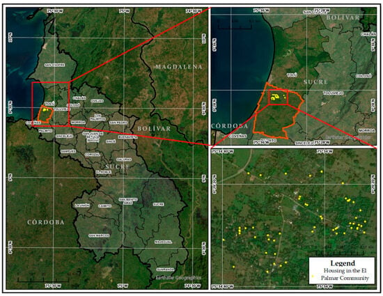
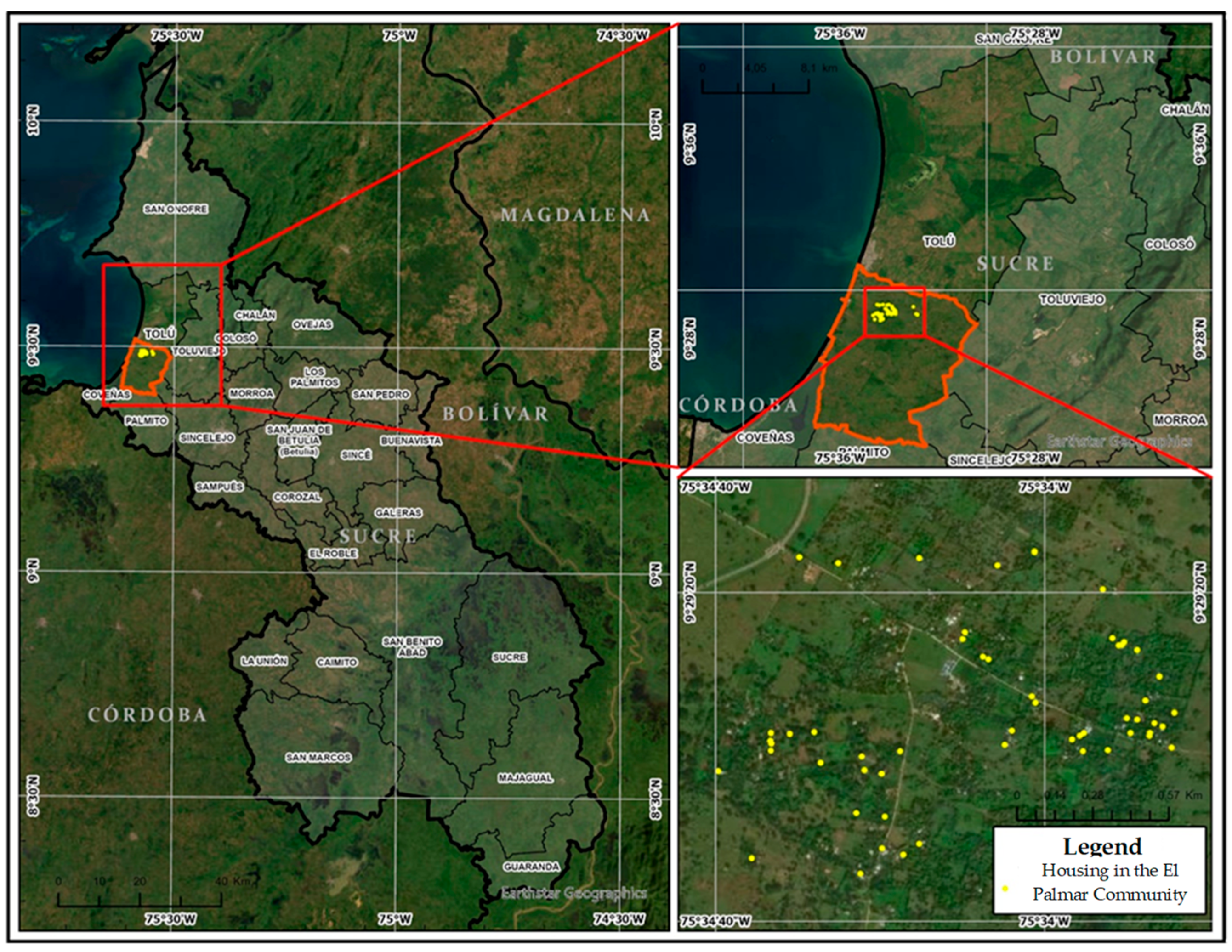
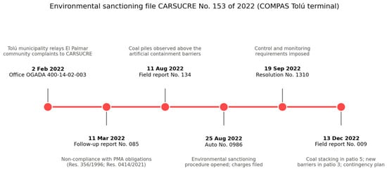
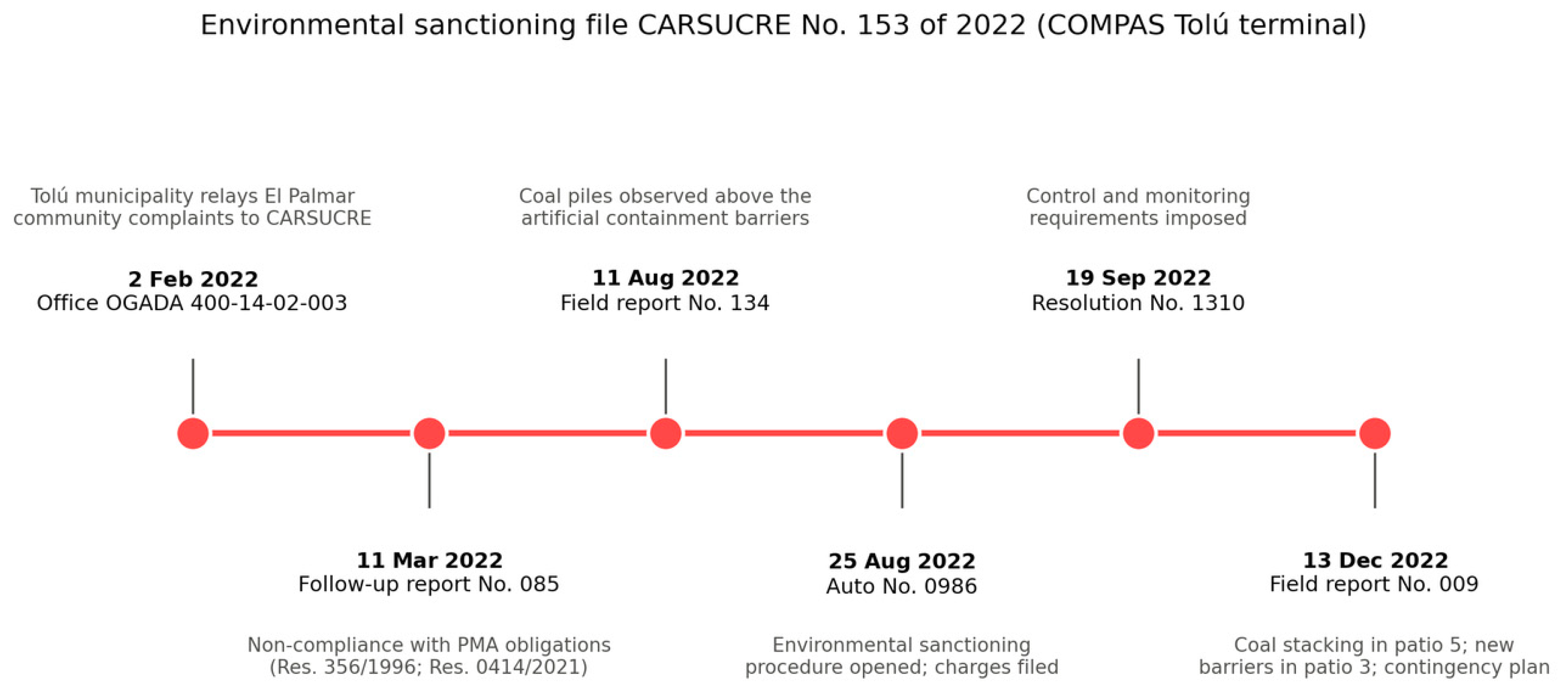
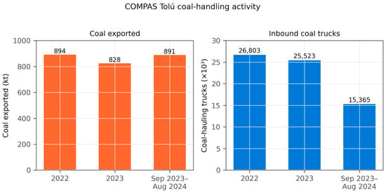
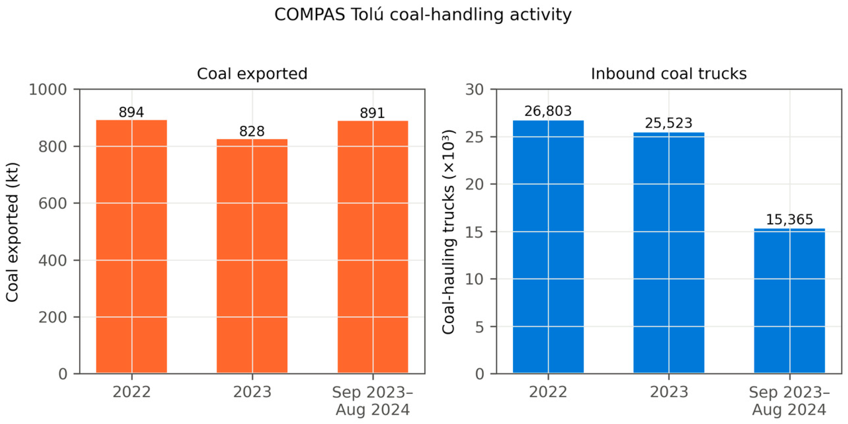
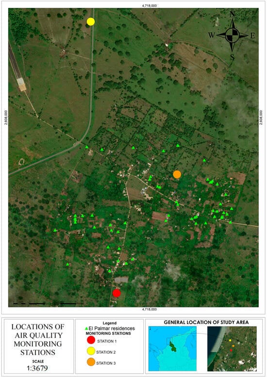
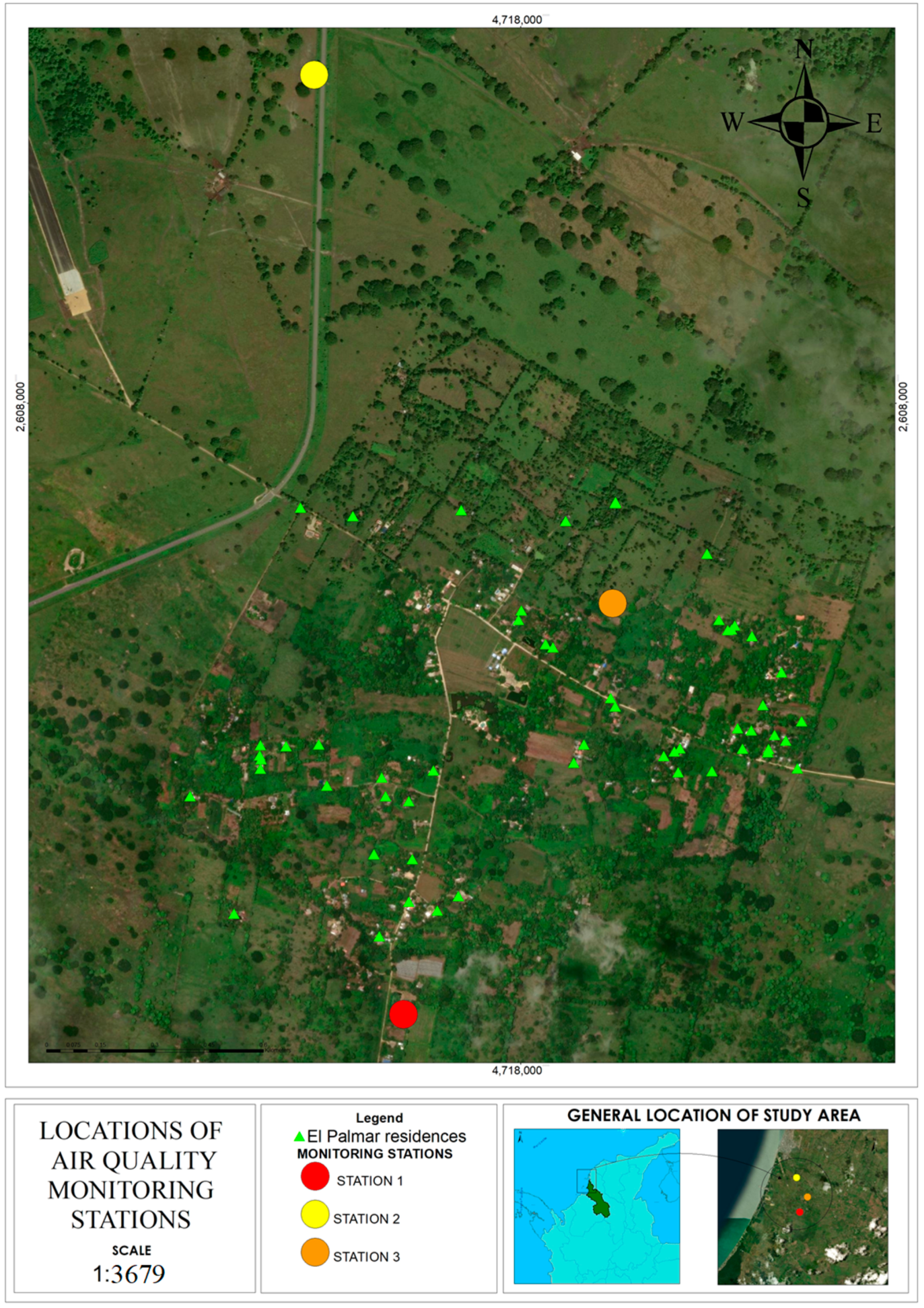
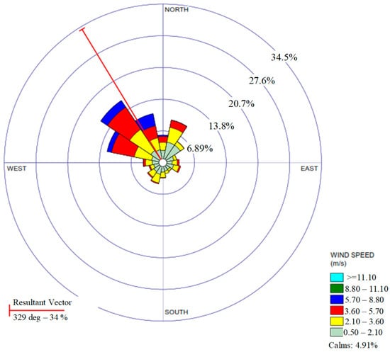
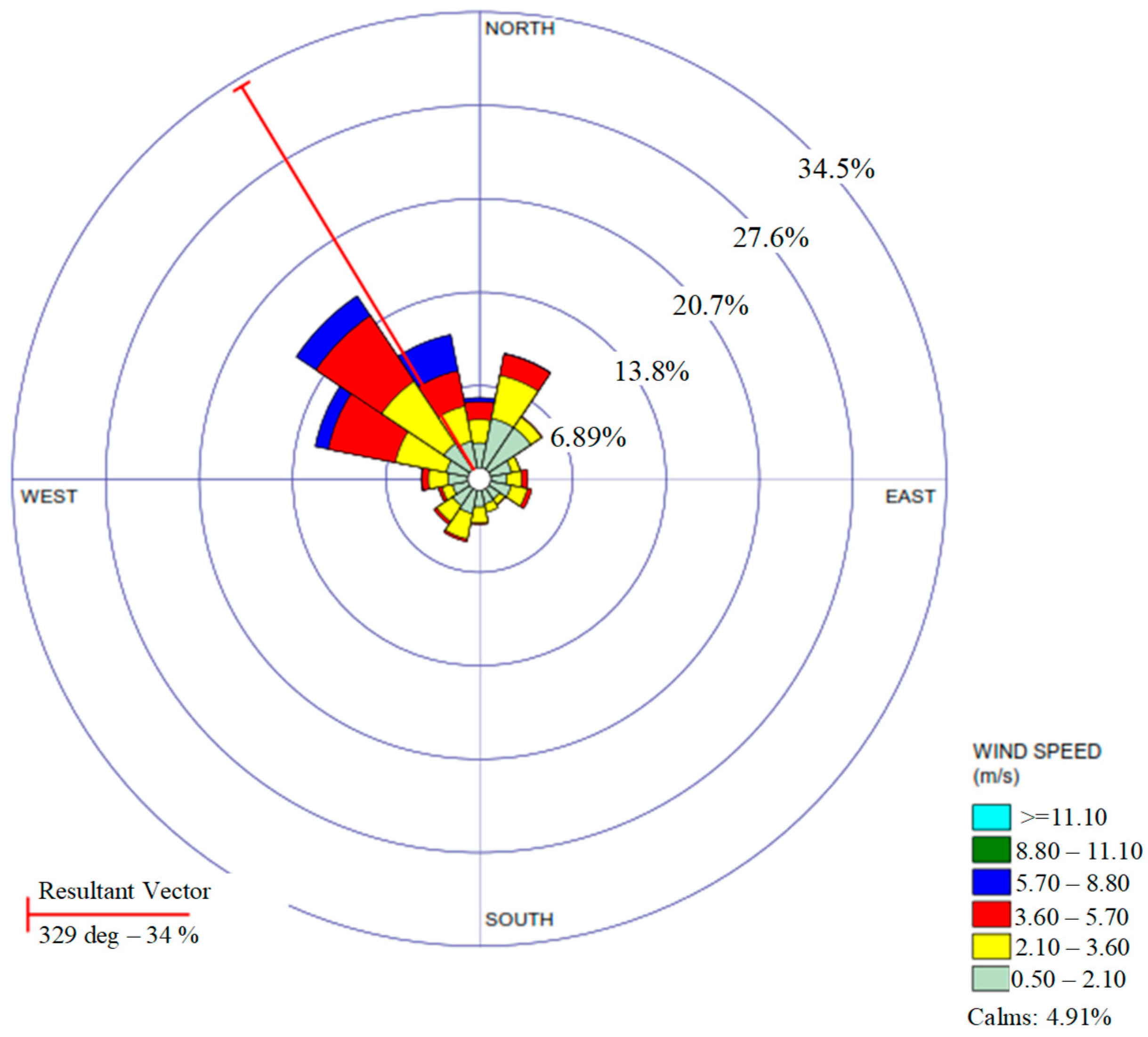
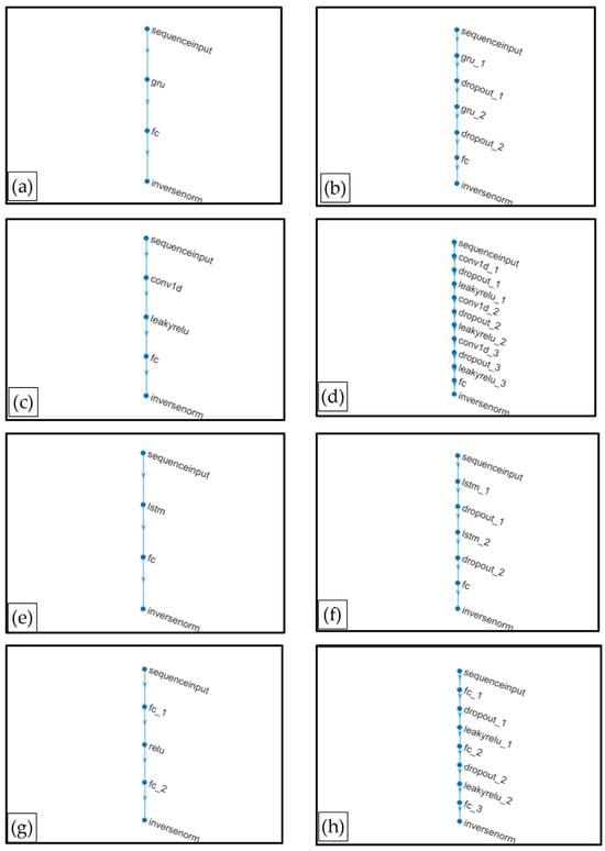
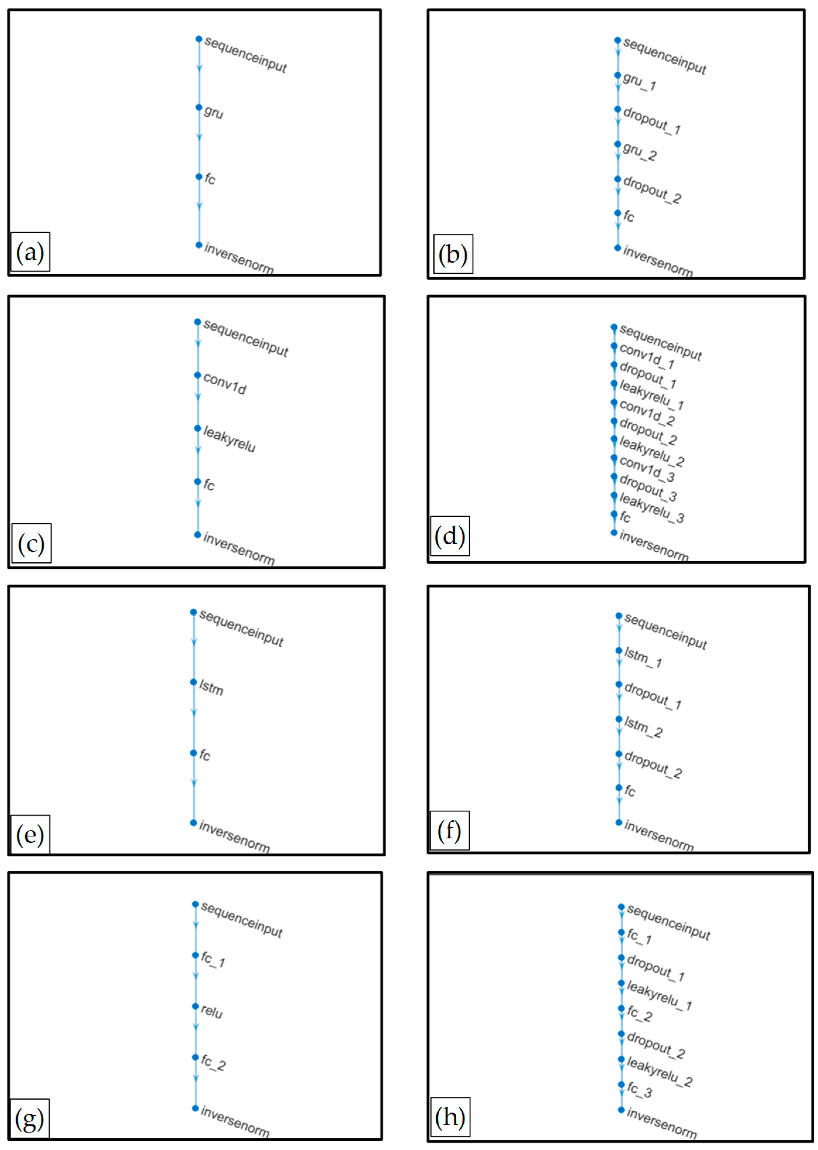
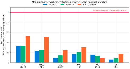
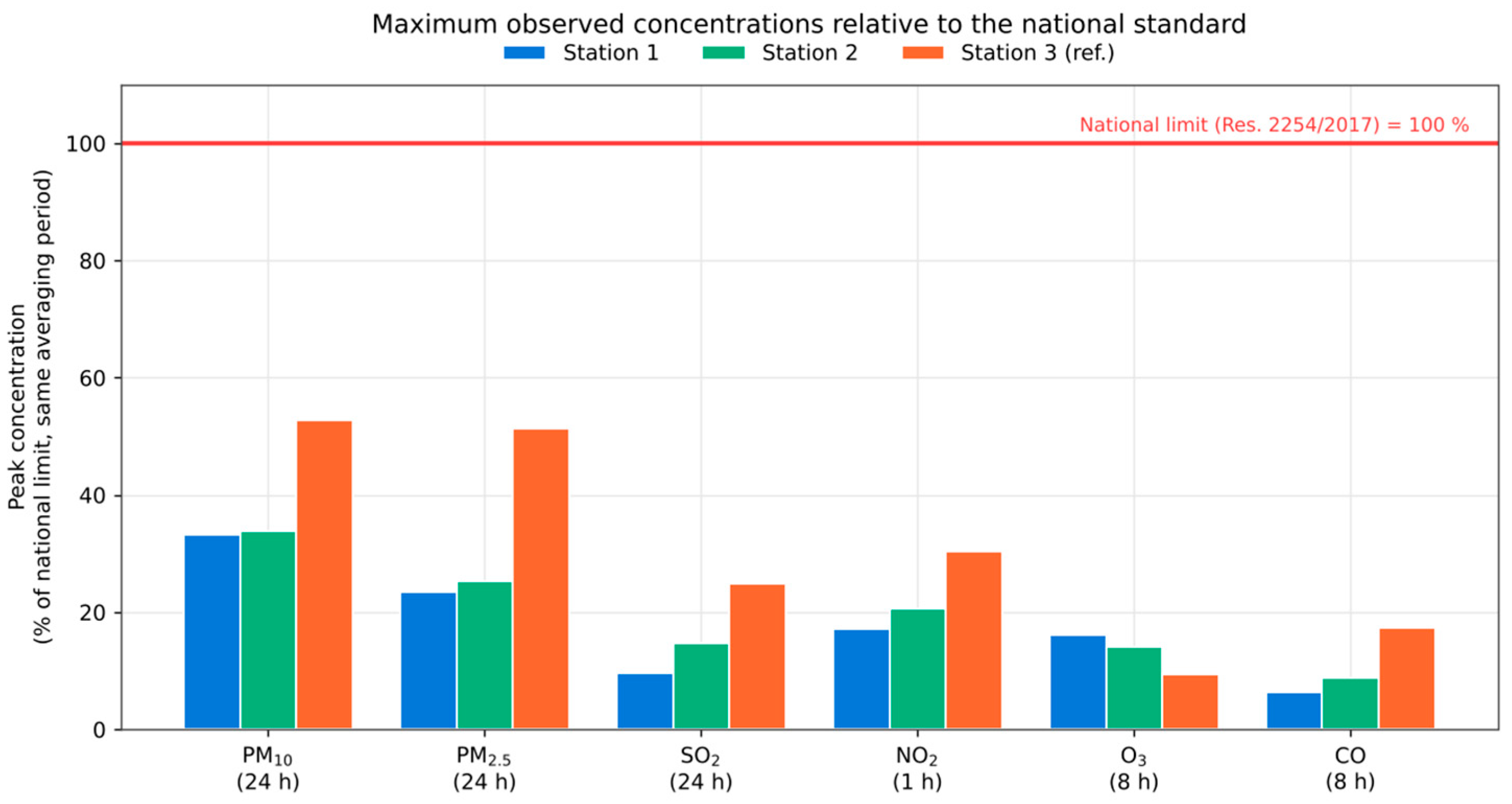
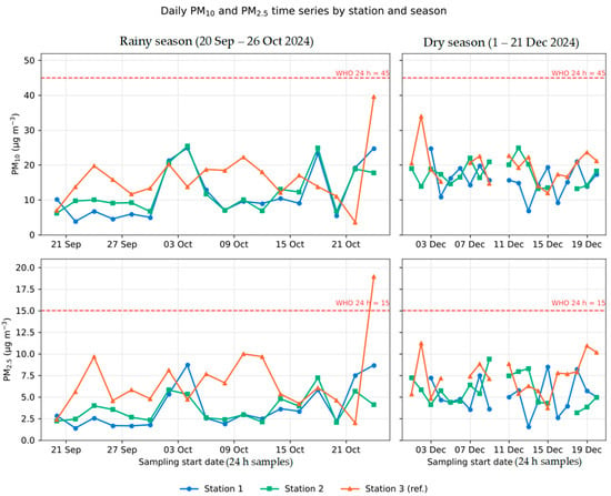
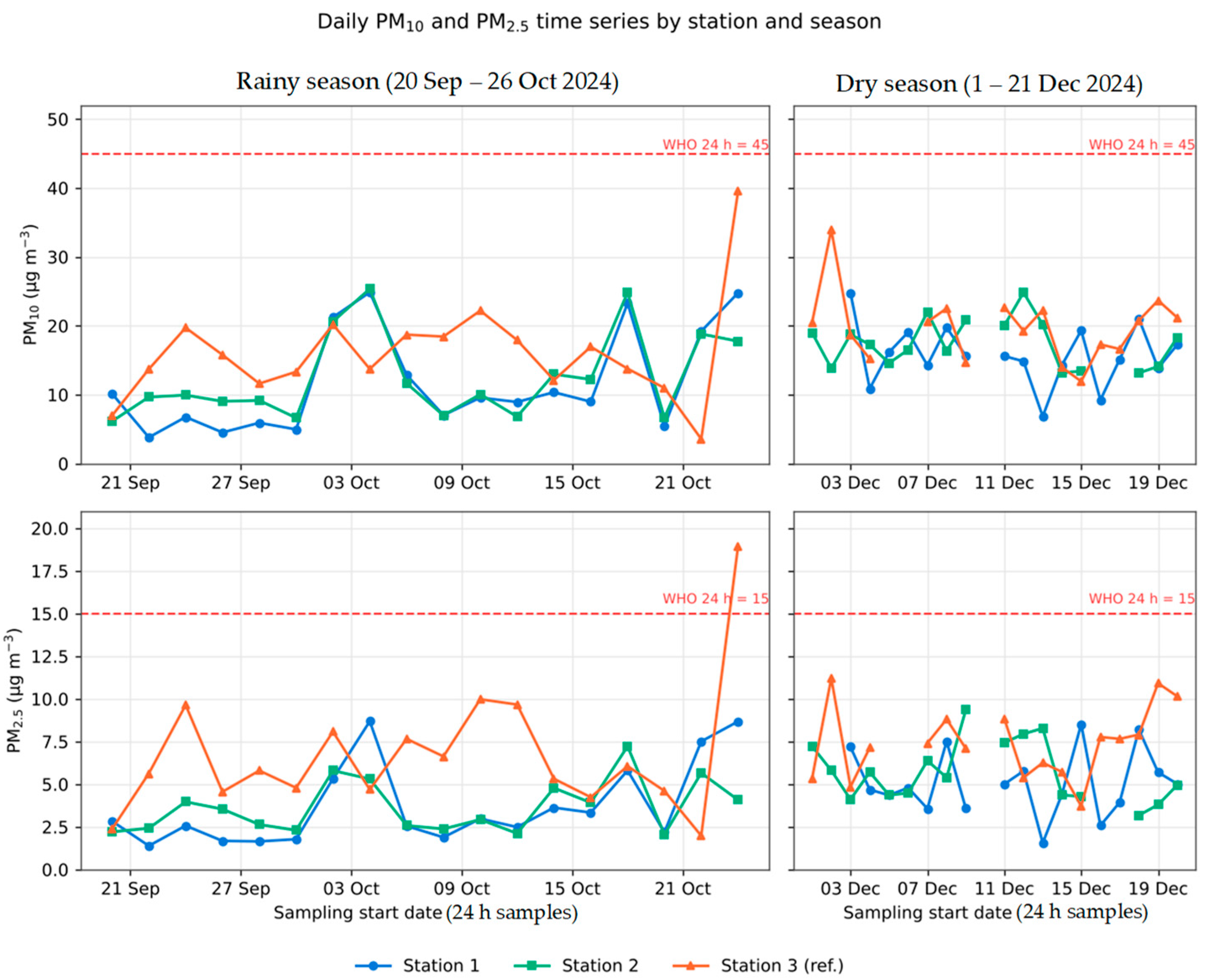
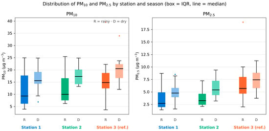
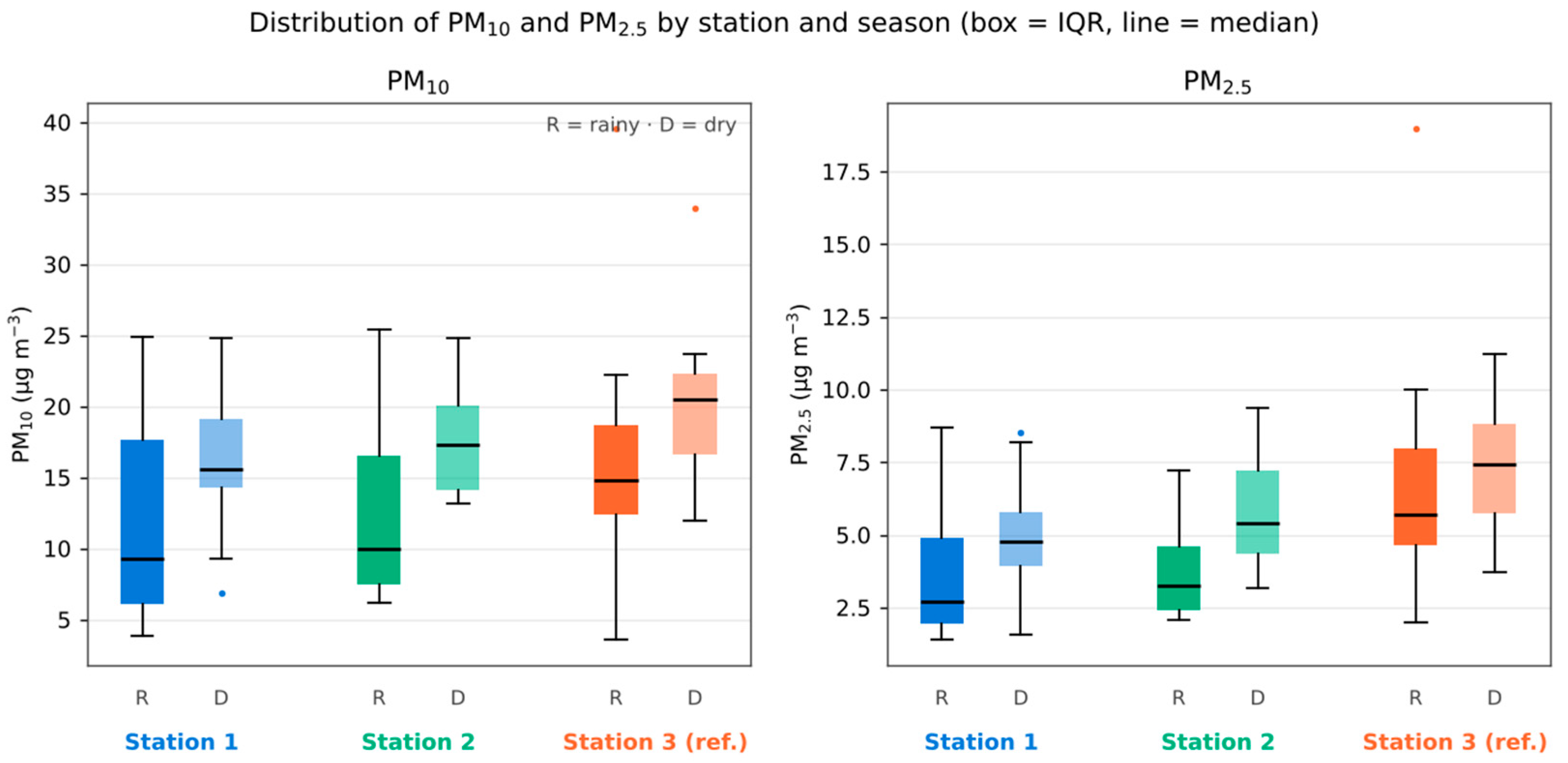
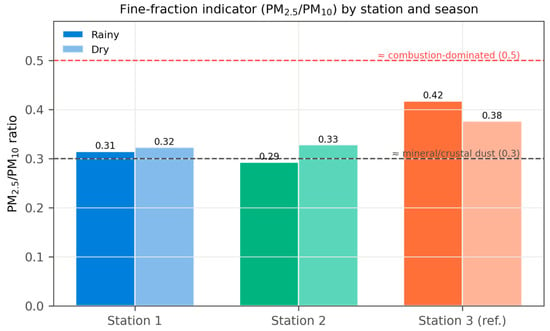
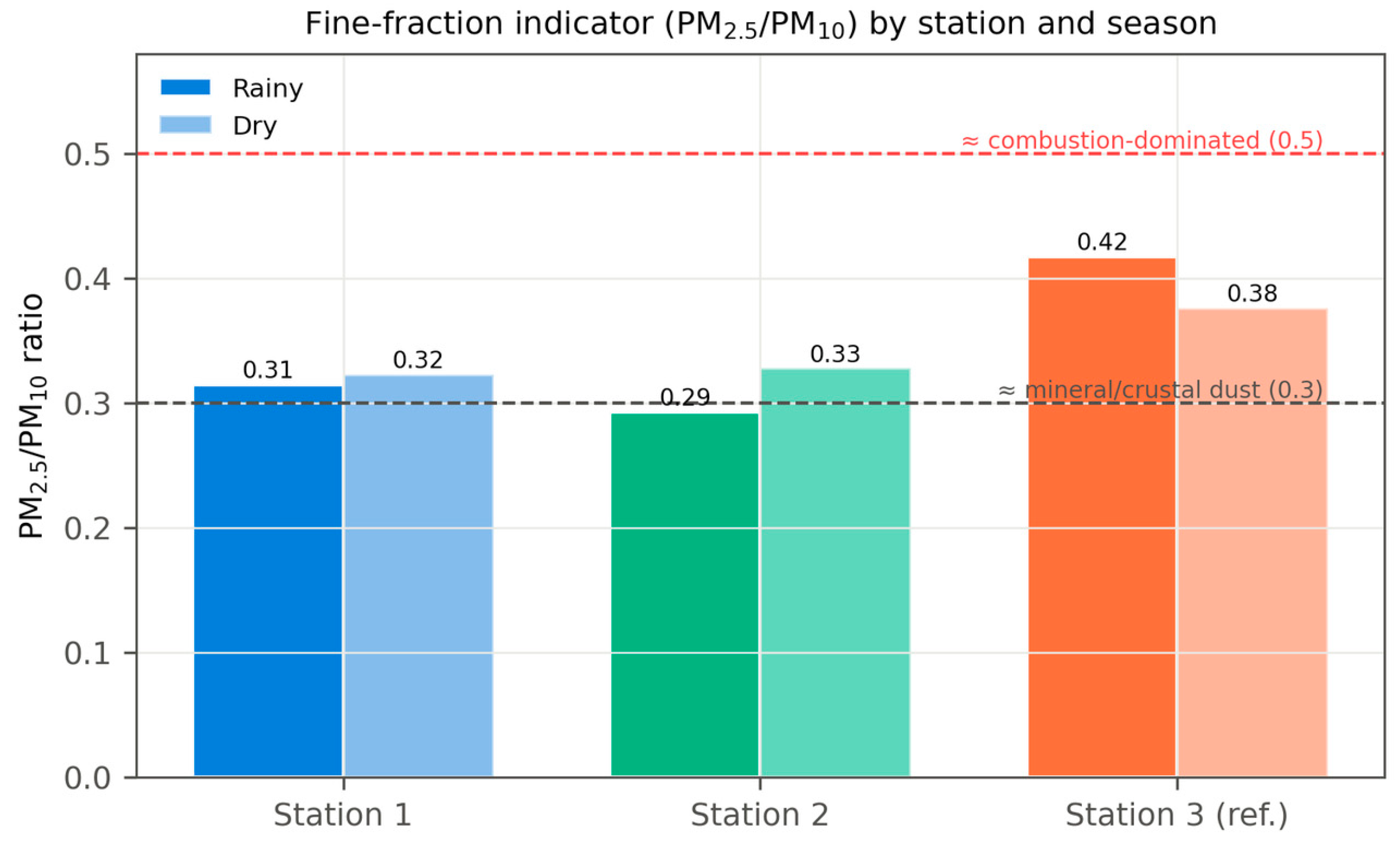
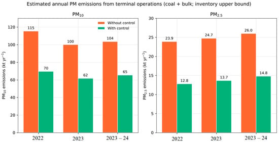
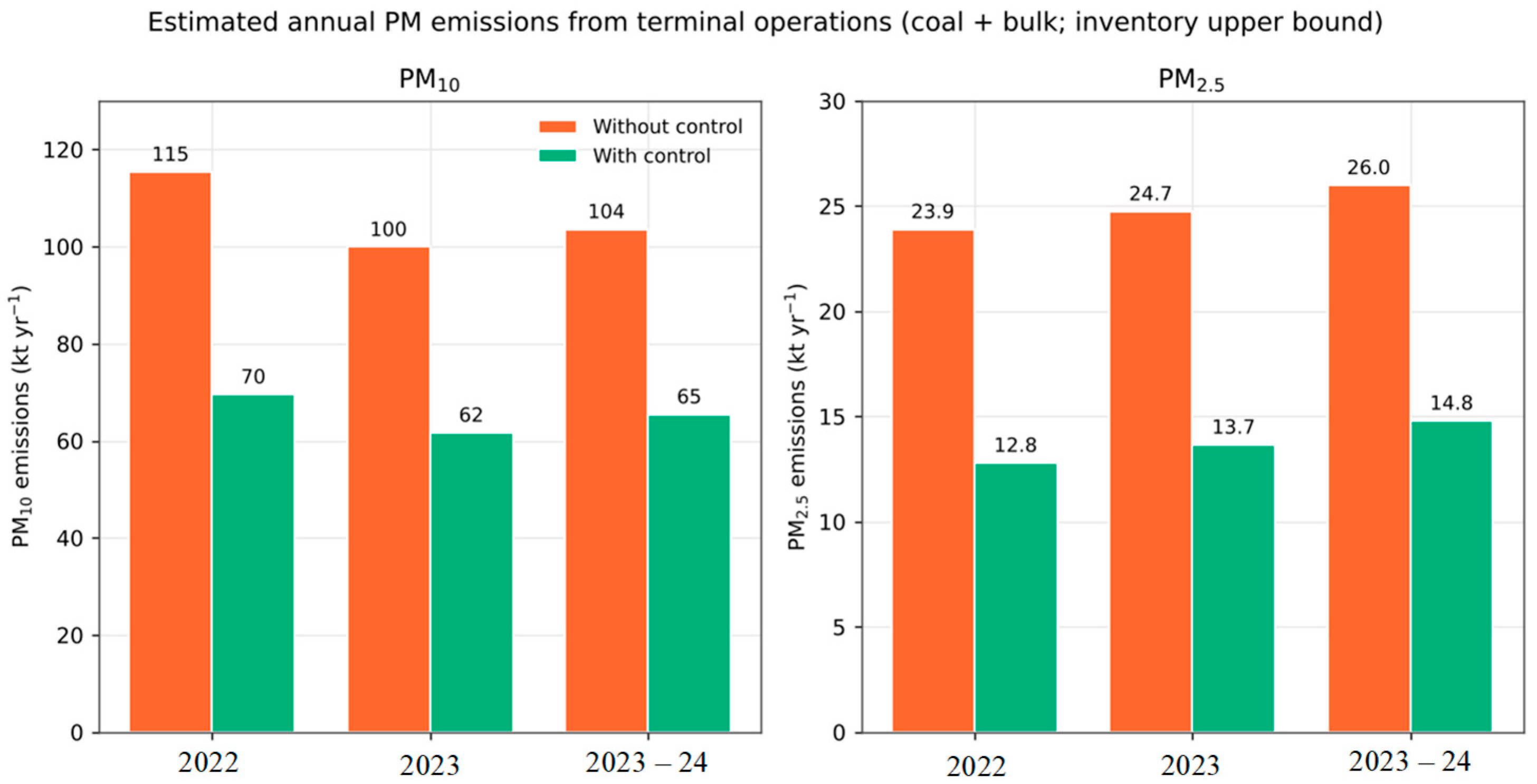
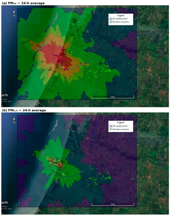
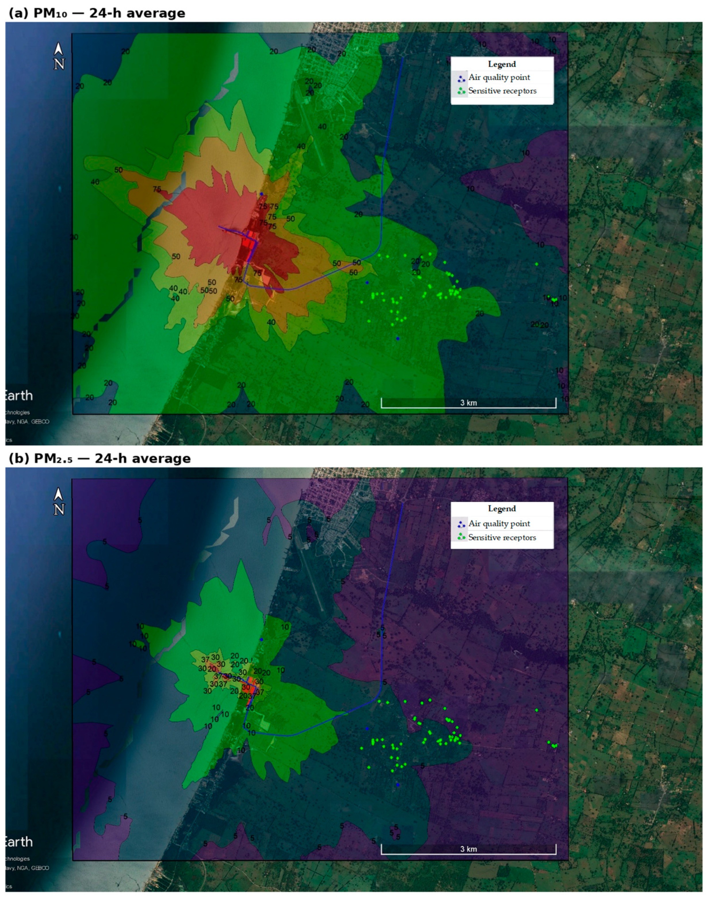
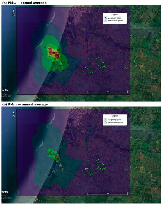
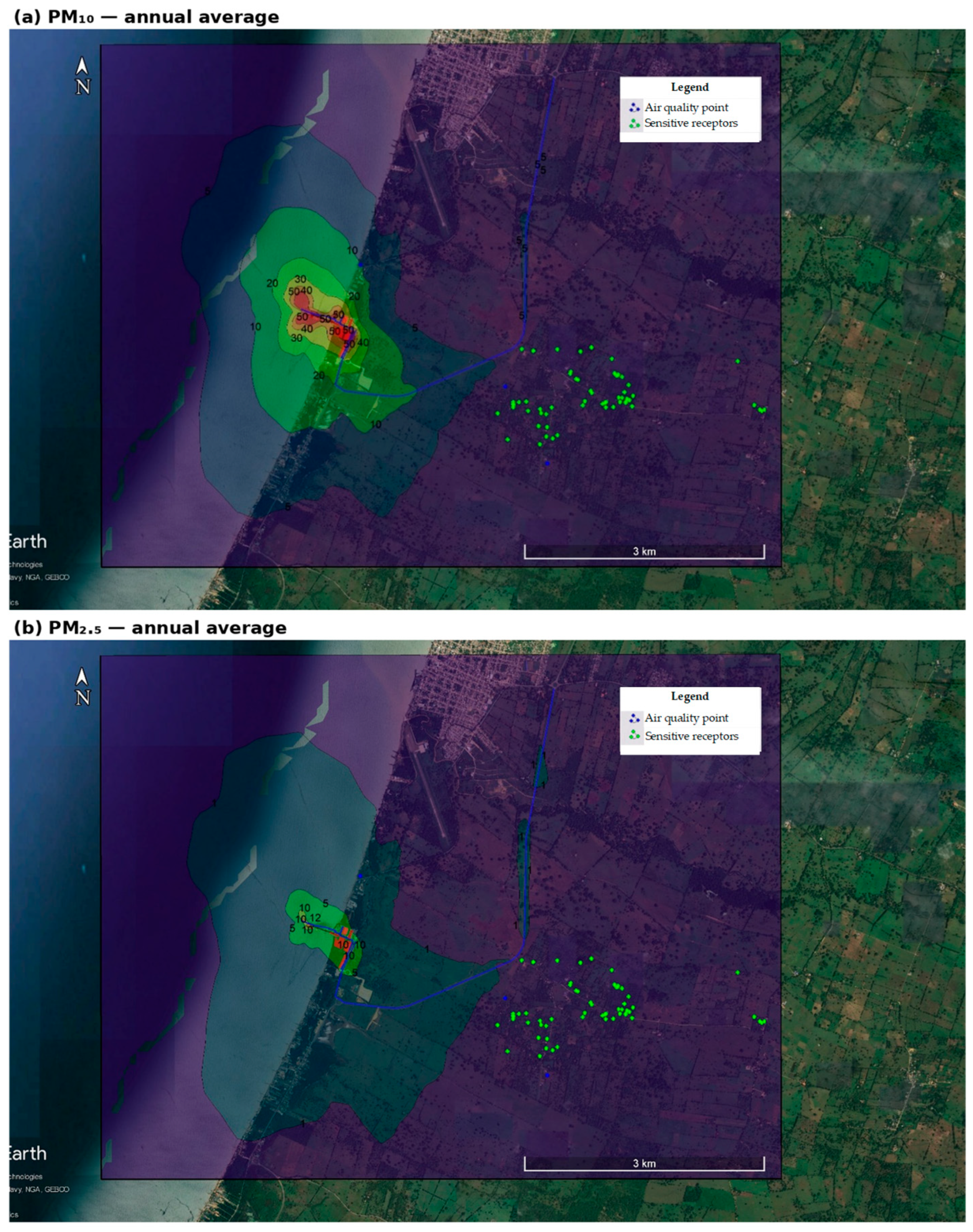
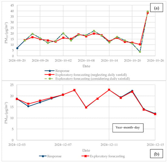
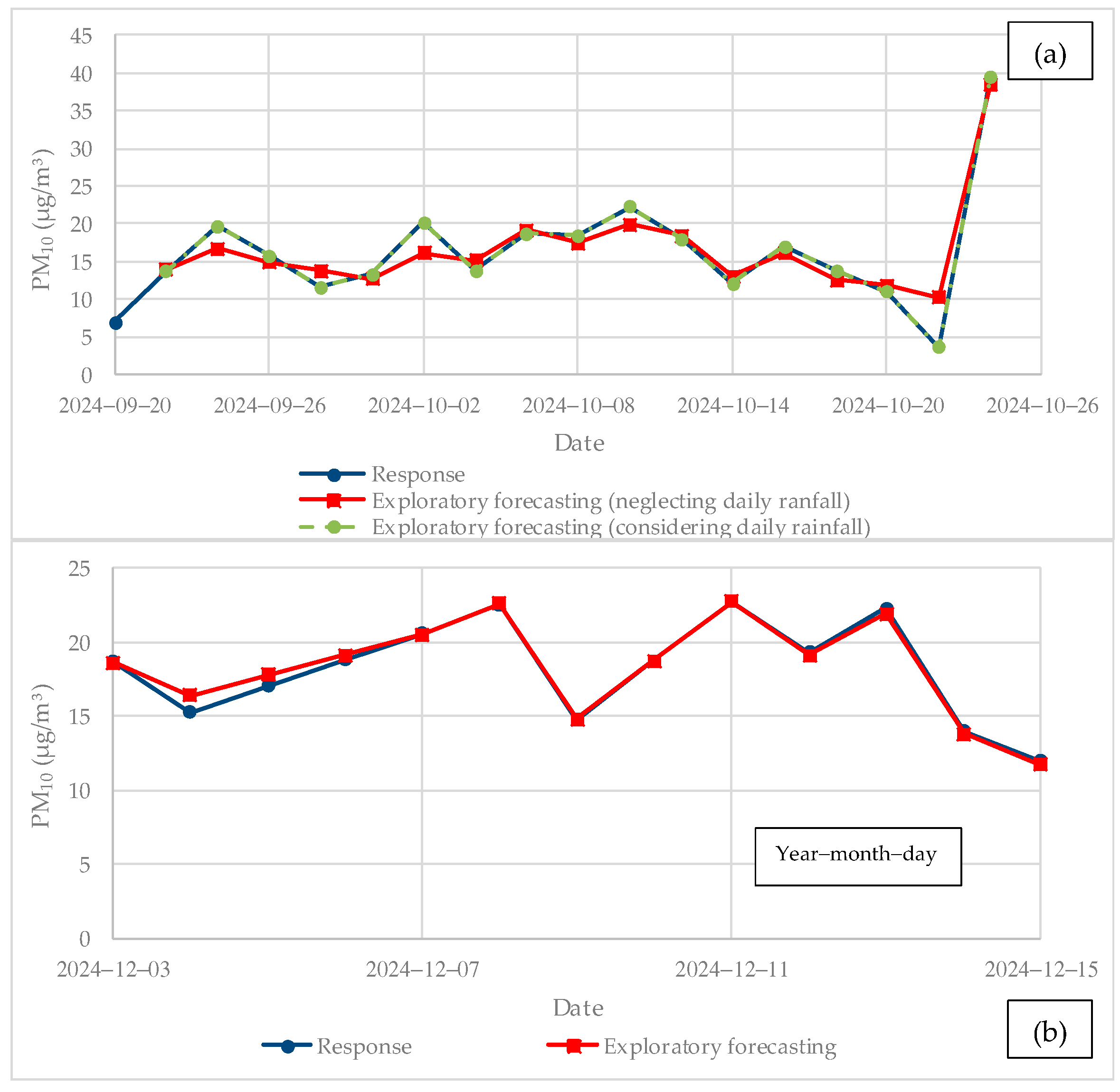
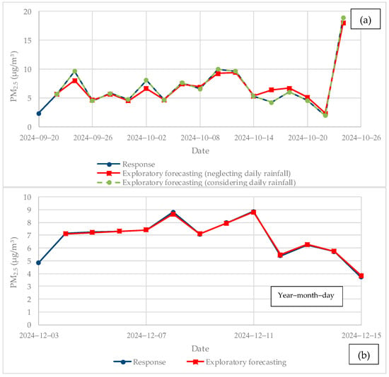

Disclaimer/Publisher’s Note: The statements, opinions and data contained in all publications are solely those of the individual author(s) and contributor(s) and not of MDPI and/or the editor(s). MDPI and/or the editor(s) disclaim responsibility for any injury to people or property resulting from any ideas, methods, instructions or products referred to in the content. |
© 2026 by the authors. Licensee MDPI, Basel, Switzerland. This article is an open access article distributed under the terms and conditions of the Creative Commons Attribution (CC BY) license.