


Abstract
Floating treatment wetlands (FTWs) are an effective nature-based solution for mitigating excess nutrient accumulation in the aquatic system. However, nutrient removal efficiency can vary significantly among plant species and seasonal conditions due to differences in plant growth, metabolism, and environmental stress response. In this study, we evaluated the nutrient removal potential of four floating plant species, including common rush (CR, Juncus effusus), three-square bulrush (TSB, Schoenoplectus pungens), tiger grass (TG, Centella asiatica), and switchgrass (SG, Panicum virgatum), during winter and spring conditions in South Texas using controlled and replicated bucket-scale experiments. Temporal reductions in total nitrogen (TN) and total phosphorus (TP) were monitored under standardized nutrient-loading conditions, and nutrient removal performance was quantified based on both concentration reduction and biomass-normalized removal. Nutrient-removal patterns differed between the winter and spring runs, and the late winter concentration increases may reflect nutrient release associated with plant stress. Despite these seasonal limitations, FTWs maintained measurable nutrient-removal capacity during the analyzed winter periods. Among the tested species, CR exhibited the highest biomass-normalized TN removal in both seasons and the highest biomass-normalized TP removal in winter; SG had the highest biomass-normalized TP removal in spring. These findings highlight the potential of FTWs for year-round nutrient management in southern US climates and identify CR as a resilient and effective species for nutrient remediation applications under variable seasonal conditions.
1. Introduction
Excessive nutrient runoff from agriculture and human activities, particularly nitrogen (N) and phosphorus (P) during rainy periods, has emerged as one of the most critical environmental challenges affecting aquatic ecosystems worldwide [1,2,3,4,5]. Major sources of nutrient pollution include agricultural runoff, livestock production systems, and municipal and urban wastewater discharges, which introduce substantial quantities of nutrients into rivers, lakes, estuaries, and wetlands [6,7,8]. When nutrient inputs exceed the natural assimilative capacity of these ecosystems, eutrophication occurs, stimulating excessive algal and aquatic plant growth and disrupting ecological balance [9]. The process can lead to harmful algal blooms, toxin production, dissolved oxygen depletion, and the formation of hypoxic or “dead zones,” ultimately causing population declines, biodiversity loss, and deterioration of overall water quality [10,11,12]. In addition to ecological impacts, nutrient pollution threatens human health, recreational water use, fisheries, and local economies. Elevated nutrient concentrations in the watershed also increase the complexity and cost of drinking water treatment and pose long-term risks to freshwater sustainability [13,14,15]. Consequently, developing effective, sustainable, and economically viable nutrient management and remediation strategies remains an urgent global priority.
Traditional nutrient removal approaches, including chemical precipitation, biological wastewater treatment in wastewater plants, and constructed wetlands, have been widely used to mitigate nutrient pollution [16,17,18,19,20,21]. Chemical precipitation using lime, alum, or iron salts can effectively remove phosphorus from wastewater; however, these approaches require continuous chemical addition, produce substantial sludge volumes, and incur relatively high operational and disposal costs [22,23,24]. Biological treatment systems, such as activated sludge processes and sequencing batch reactors, effectively remove nitrogen through nitrification and denitrification, but they often require stable operating conditions, intensive aeration, high energy consumption, and skilled personnel to maintain treatment efficiency [25,26,27,28,29]. Constructed wetlands and treatment lagoons are more sustainable, nature-based alternatives in which nutrient removal occurs through plant uptake, microbial activity, and sediment interactions [30,31,32,33]. Although these systems are generally cost-effective and environmentally friendly, they require large land areas, exhibit slower treatment performance, and are strongly influenced by environmental factors such as temperature, seasonal variation, and hydraulic loading conditions [34,35]. Collectively, these limitations highlight the need for adaptable, scalable, and sustainable technologies capable of providing reliable nutrient removal across diverse environmental settings.
Floating treatment wetlands (FTWs), which use aquatic plants on floating platforms, have emerged as a promising strategy that integrates natural nutrient assimilation with engineered treatment design [36,37,38]. In FTW systems, aquatic plants directly absorb nitrogen and phosphorus into their biomass, while root-associated microbial communities further remove nutrients through nitrification, denitrification, and phosphorus sorption [39,40,41]. Compared with conventional wetlands, FTWs offer several practical advantages, including reduced land requirements, modular scalability, and the ability to be deployed directly within existing ponds, reservoirs, canals, and wastewater systems without extensive infrastructure modification [42,43,44,45,46]. FTWs also improve water quality by stabilizing sediments, reducing light penetration and algal growth, and creating habitat for aquatic organisms. In addition, these systems generate harvestable plant biomass that can be converted into value-added products such as compost, biofertilizers, animal feed, or bioenergy feedstocks, supporting circular bioeconomy and resource recovery concepts. Beyond their environmental and economic benefits, FTWs can enhance the visual and ecological quality of aquatic environments, increasing public acceptance and promoting community engagement in sustainable water management practices. Recent work has also integrated carbon nanotube-modified anodes with ecological floating-bed microbial electrochemical systems to improve interfacial electron transfer and pollutant removal [47].
Many previous studies on floating treatment wetlands (FTWs) have focused on nutrient removal performance during summer or warm seasons, when plant growth, microbial activity, and nutrient uptake rates are typically highest. However, in southern regions of the United States (US), including Texas, several aquatic plant species remain viable and metabolically active throughout winter and early spring, potentially enabling continued nutrient removal during cooler periods. Seasonal variations in temperature, sunlight availability, and plant physiological activity can substantially influence nutrient assimilation, biomass accumulation, and overall FTW treatment efficiency. Despite the importance of year-round water treatment, limited information is available on the comparative performance of FTW plant species under winter and early spring conditions in subtropical climates.
During winter, floating treatment wetland plants shift from growth to maintenance physiology: photosynthetic rates, transpiration, nutrient uptake, and root growth all decline as carbon is reallocated to respiration and stress-protection pathways (e.g., accumulation of compatible solutes, antifreeze proteins, and changes in membrane lipid composition). Reduced enzyme activity (lower Vmax for key nutrient-assimilation enzymes and slowed transporter kinetics) and smaller root surface area both limit uptake rates for nitrogen and phosphorus. Root exudation and associated rhizosphere oxygenation also decrease, altering microbial processes (nitrification, denitrification, and organic-P mineralization) that contribute to overall system nutrient removal.
During southern Texas winters, many floating species survive but operate at reduced metabolic intensity compared with summer. Species differ in cold tolerance and acclimation capacity: some maintain higher photosynthetic quantum yields and root activity at lower temperatures, while others rapidly downregulate growth and assimilatory pathways. These differences drive species-specific nutrient-removal performance under cold conditions. In this study, we evaluated different eco-physiological strategies, such as allowing acclimation periods (weeks) to avoid transient handling effects and assessing recovery potential when temperatures rise for four plants (CR, TSB, TG, SG).
In this study, we evaluated and compared the nutrient removal efficiency and biomass production of four aquatic plant species, including common rush (CR, Juncus effusus), three-square bulrush (TSB, Schoenoplectus pungens), tiger grass (TG, Centella asiatica), and switchgrass (SG, Panicum virgatum), grown under simulated Texas wetland conditions during winter and early spring. We monitored changes in total nitrogen (TN) and total phosphorus (TP) removal alongside plant growth performance to better understand seasonal treatment dynamics under cooler environmental conditions. The findings aim to identify robust aquatic plant species capable of maintaining effective nutrient removal during lower-temperature periods and to provide insights for optimizing FTW design and management strategies for reliable, year-round wastewater and stormwater treatment applications in southern US climates.
2. Materials and Methods
2.1. Floating Plant Preparation
Before the seasonal nutrient-removal experiments, we removed the original potting soil from the plant-holder cups. Commercially purchased plants were removed from their pots and rinsed with a gentle water jet to remove residual soil and adhered nutrients (Figure S2). Roots were thoroughly washed, and plants were then placed in soil-free holder cups and floated on water for 3–4 weeks before the formal experiment. This recovery period allowed plants to recover from handling stress and stabilize physiologically, ensuring that measured nutrient removal reflected uptake from the test medium rather than residual soil-derived nutrients.
2.2. Experimental Design
2.2.1. Plant Selection for Nutrient Removal
Four locally relevant species were tested in a replicated bucket system: common rush (CR, Juncus effusus), three-square bulrush (TSB, Schoenoplectus pungens), tiger grass (TG, Centella asiatica), and switchgrass (SG, Panicum virgatum). The experiments used 5-gallon HDPE buckets (S-14960; Uline, Pleasant Prairie, WI, USA; height 36.8 cm, outside top diameter 30.2 cm, and outside bottom diameter 26.0 cm), each containing 10 L of nutrient solution [48]. Plants were supported in holder cups in a floating mat (Figure S1), with approximately 20% surface coverage. Individual plants were not counted; plant loading was characterized by total fresh weight measured at the start and end of the experiment (Section 2.2.3). Three independent replicate buckets were used per species (n = 3), with each bucket serving as the experimental unit.
2.2.2. Nutrient Level Control
The nutrient solution was prepared using Southern Ag PowerPak 20-20-20 water-soluble fertilizer (Southern Agricultural Insecticides, Inc., Palmetto, FL, USA), containing 20.0% TN and 20.0% available phosphate as P2O5 (8.73% elemental P) by weight. Its main nutrient sources were potassium nitrate, monoammonium phosphate, diammonium phosphate, and urea, with added micronutrients. At the start of the experiment, the fertilizer was dosed to 0.3 g L−1, resulting in initial concentrations of 60 mg L−1 total nitrogen and 26.5 mg L−1 total phosphorus in each bucket. The same starting nutrient loading was used for all species to provide a common basis for comparison. Because evaporation and plant water uptake reduced the solution volume between weekly samplings, water-level changes were monitored by photographing each bucket and estimating the remaining volume with a Python script. At the end of each week, the remaining solution volume and the corresponding TN and TP concentrations were determined before replenishment. These paired measurements were used to correct the TN and TP removal calculations for changes in solution volume caused by evaporation and plant water uptake. After sampling and volume measurement, nutrient-free water was added to restore each bucket to 10 L. Evaporation and plant water uptake were not measured separately. A fixed measuring scale inside each bucket will be used in future experiments to improve the direct measurement of solution volume.
2.2.3. Plant Nutrient Removal Efficiency Measurements
Plant responses were tracked as biomass and morphology. Total fresh weight was measured at the start and end of the study to determine net biomass change. Weekly shoot and root lengths were quantified from photographs using Python 3.0 image analysis with OpenCV 5.0.0 to extract linear dimensions (Figures S3–S6). These measurements, combined with standardized nutrient dosing, explicit volume accounting, and independent bucket replicates, provide a consistent basis for comparing winter and spring nutrient-removal performance among the four species.
2.3. Nutrient Level Evaluations
2.3.1. Instrumentation
Water samples from the bucket experiment (four species; see Section 2.2) were analyzed for total nitrogen (TN) and total phosphorus (TP) using a GNST-900S (Henan Suijing Environmental Protection Technology Co., Ltd., Luoyang, China) multi-parameter colorimeter (Figure S9a). Samples were digested prior to analysis with a GENESITE SJ-16X (Henan Suijing Environmental Protection Technology Co., Ltd., Luoyang, China) rapid digester (16-position block; Figure S9b). Assay-specific reagents and standards are summarized in Figure S9c. The detailed TN and TP analytical procedures are provided in Supplementary Tables S1 and S2.
2.3.2. Reagents Used and Quality Control
TN and TP reagents were freshly prepared according to the manufacturer’s instructions. For TN: Reagent I (TN reagent powder dissolved in Reagent Liquid I), Reagent II (powder dissolved in distilled water), and Reagent III (concentrate mixed with sulfuric acid). For TP: Reagent I (TP reagent dissolved in distilled water), Reagent II (dissolved in a small volume of distilled water), and Reagent III (used as supplied). Distilled water was used for dilutions, blanks, and rinses. Calibration standards, method blanks, and quality-control samples (matrix spikes or duplicates, when applicable) were run each analysis day in accordance with the instrument manufacturer’s protocol.
2.3.3. TN Analysis
TN was determined using the GNST-900S manufacturer’s alkaline persulfate digestion photometric method [49]. The sample preparation, digestion, and color-development steps followed the manufacturer’s protocol and are summarized in Supplementary Table S1. Samples were analyzed within the method’s working ranges. For the 0–20 mg L−1 range, 2.0 mL of sample was used directly; for the 20–100 mg L−1 range, 0.40 mL of sample was diluted to 2.0 mL with distilled water. To each tube, add 1.0 mL of Reagent I, cap, mix, and digest at 125 °C for 30 min in the SJ-16X. After cooling to room temperature, add 0.50 mL of Reagent II, mix, then add 4.0 mL of Reagent III, shake, and allow the color to develop for 15 min. Measure absorbance on the GNST-900S and calculate TN using the day’s calibration curve.
2.3.4. TP Analysis
TP was determined using the GNST-900S manufacturer’s ammonium molybdate photometric method, based on GB/T 11893-1989 [49,50]. The instrument-specific procedure, including digestion and color development, is described below and summarized in Supplementary Table S2. For the 0–2 mg L−1 range, use 5.0 mL of sample; for 2–20 mg L−1, dilute 0.50 mL of sample to 5.0 mL with distilled water (0.50 mL of sample + 4.5 mL of water). Add 1.0 mL of Reagent I, cap, mix, then digest at 125 °C for 30 min. After cooling, add 4 drops of Reagent II and mix; then add 6 drops of Reagent III and mix; allow the color to develop for 10 min. Measure absorbance on the GNST-900S and determine TP from the calibration curve.
2.3.5. Data Handling
Daily calibration curves were used to convert absorbance to concentration. Results were corrected for dilution factors and compared with blanks and QC samples; values that failed QC were reanalyzed. Final concentrations reported for subsequent statistical analysis were blank-corrected and dilution-adjusted for TN and TP. In addition to analytical dilution corrections, TN and TP removal calculations accounted for the remaining solution volume determined at each weekly sampling. This adjustment accounts for the combined concentration effect of evaporation and plant water uptake; it does not separate nutrient uptake from other removal or release pathways.
3. Results and Discussion
3.1. Artificial Soil (Vermiculite) Effect
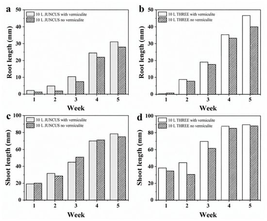
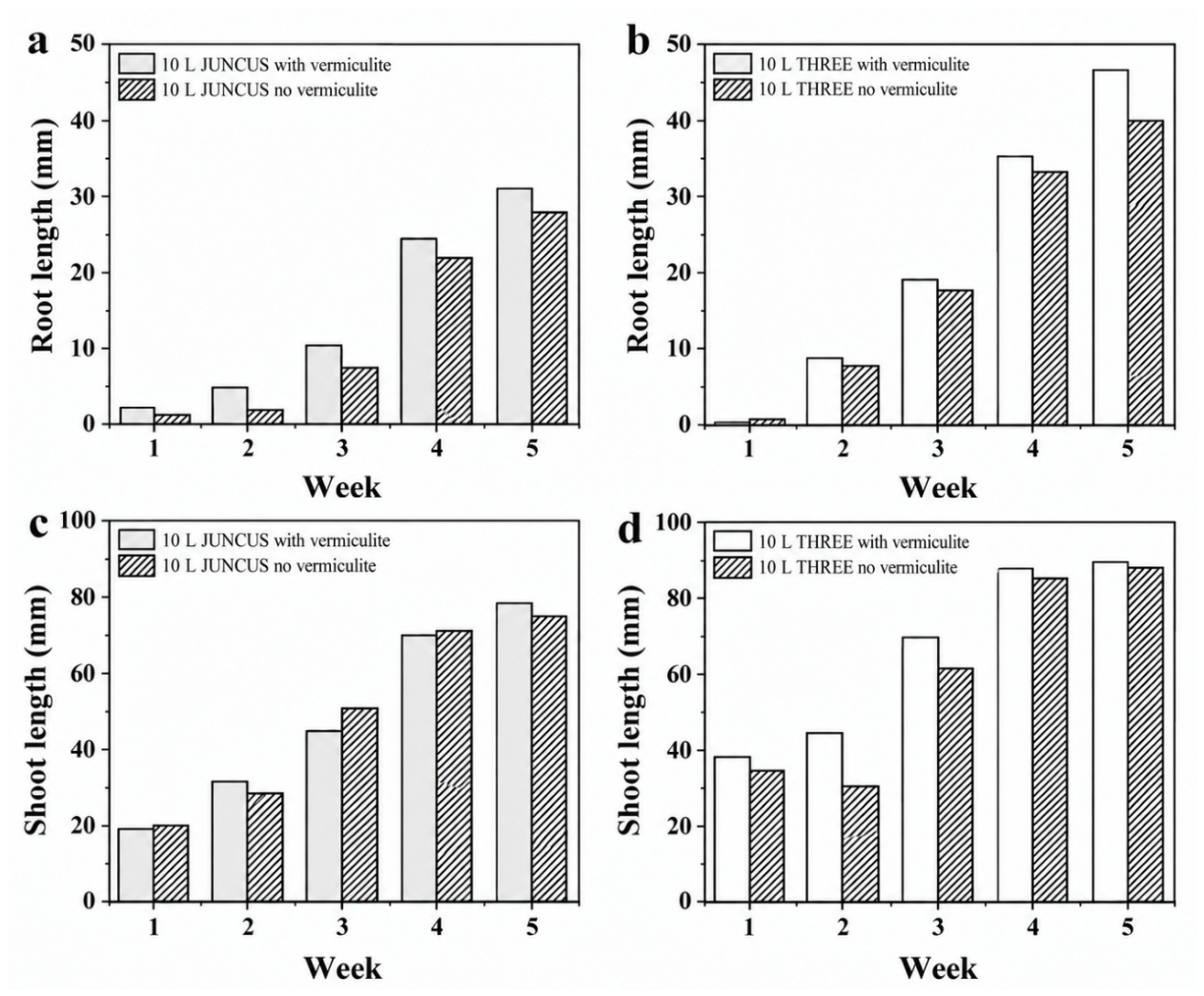
We assessed root and shoot growth of CR and TSB over five weeks by comparing plants in holder cups without soil or vermiculite with plants in holder cups containing horticultural vermiculite. This preliminary comparison assessed whether adding a substrate was necessary for the selected configuration; alternative support materials were not compared. The subsequent seasonal nutrient-removal experiments used washed plants in holder cups without soil or vermiculite. Preliminary tests with CR and TSB considered water volumes of 5 L and 10 L over five weeks. The experiment used 5-gallon buckets, with water volumes of 10 and 5 L corresponding to water depths of 18 and 9 cm, respectively. At the end of each week, the water level was measured to estimate the combined volume change associated with evaporation and plant water uptake.
Figure 1 shows the preliminary comparison with and without vermiculite. Differences were small for both species. After five weeks, vermiculite increased root length modestly (~10% for CR and ~18% for TSB) but had a negligible effect on shoot growth; by week five, shoot lengths were essentially identical between treatments. Thus, vermiculite provided only a minor benefit to roots and did not affect overall development; consequently, all subsequent experiments were performed without artificial soil to simplify the setup and avoid potential confounding factors.
Figure 1.
Preliminary comparison of root and shoot growth with and without horticultural vermiculite at a water volume of 10 L. Panels a and c show common rush (CR, Juncus effusus), and panels b and d show three-square bulrush (TSB, Schoenoplectus pungens). Unhatched bars indicate vermiculite and diagonally hatched bars indicate no vermiculite. Root length is shown in (a,b) and shoot length in (c,d) over five weeks. In the panel legends, “JUNCUS” and “THREE” denote CR and TSB, respectively, and “with vermiculite” and “no vermiculite” indicate the presence and absence of vermiculite.
3.2. Nutrient Removal Efficiency in the Winter of Texas
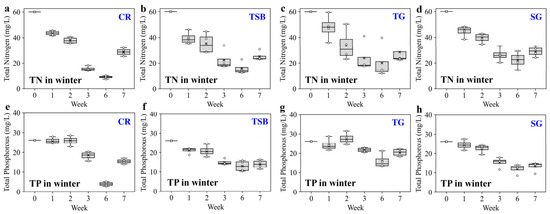
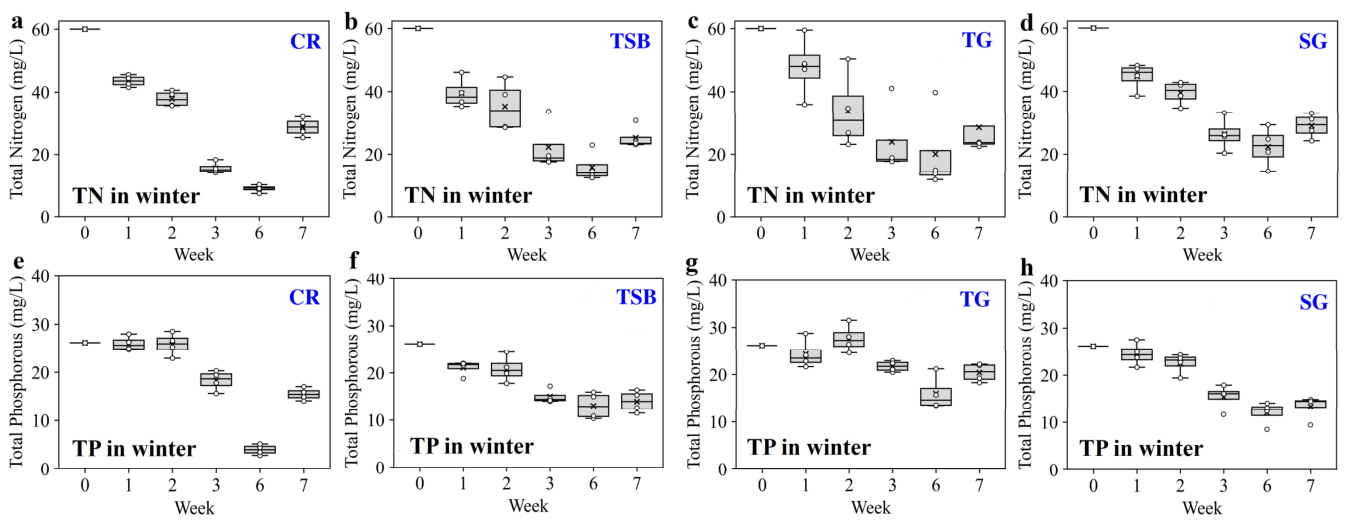
Figure 2a–h summarizes winter TN and TP concentrations for the four species. The experiment began in the first week of December 2024. To avoid freezing damage, all buckets were moved indoors for approximately three weeks; visible plant stress was qualitatively noted during this interval, and data from the indoor period were excluded from the analysis. Indoor air temperature was approximately 25 °C, and illumination was provided by overhead ceiling lights. Plant stress was assessed visually; no quantitative stress index was measured, and reduced light remains a possible explanation. The winter run therefore does not represent continuous outdoor exposure. Additional regional temperature context is provided in the Supporting Information section “Regional temperature context” (Figure S7 and Table S3) [51]. Continuous indoor temperature records and quantitative measurements of bucket-water temperature and irradiance were unavailable, limiting direct evaluation of their relationships with nutrient removal.
Figure 2.
Winter changes in total nitrogen (TN) (a–d) and total phosphorus (TP) (e–h) concentrations in the experimental buckets. The columns show common rush (CR, Juncus effusus) (a,e), three-square bulrush (TSB, Schoenoplectus pungens) (b,f), tiger grass (TG, Centella asiatica) (c,g), and switchgrass (SG, Panicum virgatum) (d,h). Each species was tested in three independent replicate buckets (n = 3), with a 10 L working solution volume. TN and TP concentrations are expressed in mg L−1; nutrient-removal calculations accounted for the corresponding weekly solution volumes. Box-and-whisker plots with overlaid measurements summarize weeks 0, 1, 2, 3, 6, and 7 as separate sampling categories; connecting lines are not used. Weeks 4 and 5 are not shown because data from the temporary indoor period were excluded, and nutrient changes during that interval cannot be resolved from this figure.
Across the analyzed outdoor periods, CR showed the greatest overall TN reduction and SG the weakest removal, with TSB and TG showing intermediate performance. TP followed species-specific trends (Figure 2e–h), with CR showing the largest overall decrease; absolute TP values and temporal patterns varied across sampling dates. Note that observed nutrient removal reflects both uptake activity and standing biomass; the influence of biomass on removal efficiency is examined in a later section.
TN removal rate was not constant over time. Week 1 showed the highest TN removal, driven by relatively high initial TN concentrations. Week 3 also exhibited comparatively high removal. No observations at weeks 4 and 5 are displayed, so nutrient dynamics during the indoor interval cannot be resolved from the plotted series. In week 7, TN concentrations increased after the plants had been returned outdoors. Decomposition of plant material has been shown to increase water-column TN during winter, while seasonal tissue turnover can release P in floating wetlands [52,53]. Nutrient release from stressed or senescent tissues may therefore temporarily offset removal and contribute to the week-7 rebound. This remains a possible explanation because tissue nutrient release was not directly measured here.
Figure 2e–h shows TP dynamics over the same winter period. Unlike TN, TP responses were more gradual. During weeks 0–3, TP remained relatively stable across treatments. TP concentrations were lower after the sampling gap, but the displayed observations do not establish when the decrease occurred during that interval. TP removal differed among species, with CR showing the strongest overall performance. The measured TN and TP decreases represent net nutrient removal from the water and cannot be attributed to plant assimilation alone. The use of soluble fertilizer and washed plants without soil or vermiculite limited the initial input of settleable solids. Floating-mat and tap-water control measurements after three weeks are shown in Figure S8. Clean HDPE containers are suitable for nutrient sampling, although wall-associated microbial films can alter nutrient concentrations [54]. Phosphate adsorption to HDPE particles has been reported to be lower than to the soils tested and largely reversible, but those experiments do not quantify retention by bucket walls [55]. Sedimentation and sorption may also contribute to phosphorus removal in floating treatment wetlands [56]. Because wall- and sediment-associated nutrients were not measured separately, their contributions cannot be quantified in the present experiment.
3.3. Nutrient Removal Efficiency in the Spring Season
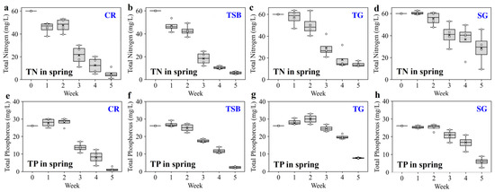
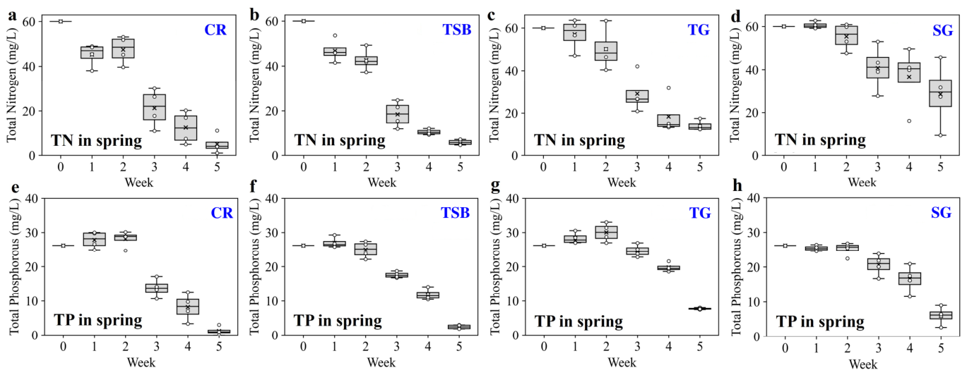
Figure 3a–d shows TN concentration changes for the different floating species during the spring season in Texas. Across all species, TN declined over the five-week run, indicating effective nitrogen removal. CR (Figure 3a) and TSB (Figure 3b) exhibited pronounced TN decreases after week 2, with TN falling from ~60 mg L−1 to below 10 mg L−1 by week 5. TG (Figure 3c) produced moderate but steady removal, ending near 15 mg L−1, while SG (Figure 3d) displayed slower kinetics and greater between-replicate variability, though net reduction was evident by the end. TN changes during the first two weeks varied among species, with larger decreases generally observed after week 2. Studies of FTW establishment report time-dependent plant and rhizosphere development, but the present measurements do not establish physiological inhibition [57]. The relationship between these spring patterns and the weather record is considered in Section 3.4.
Figure 3.
Spring changes in total nitrogen (TN) (a–d) and total phosphorus (TP) (e–h) concentrations in the experimental buckets. Columns show common rush (CR) (a,e), three-square bulrush (TSB) (b,f), tiger grass (TG) (c,g), and switchgrass (SG) (d,h). Concentrations are expressed in mg L−1 for weeks 0–5; each species was tested in three independent replicate buckets (n = 3).
Figure 3e–h presents TP dynamics for the same period. TP generally trended downward, but species-specific patterns differed from TN. CR (Figure 3e) and TSB (Figure 3f) showed strong phosphorus removal, with TP falling rapidly after week 2 to near-complete removal or below ~5 mg L−1 by week 5. TG (Figure 3g) exhibited a more gradual TP decline, stabilizing around ~8 mg L−1, while SG (Figure 3h) removed phosphorus consistently but less aggressively. Early in the experiment, TP was largely stable across most species; TG even showed a slight, transient increase in TP, potentially reflecting short-term P release during acclimation; the contributing processes were not measured. Root-zone sorption, microbial P immobilization, and biofilm uptake are possible contributors to the sustained TP declines after week 2.
3.4. Seasonal Comparisons
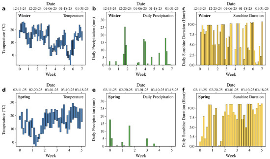
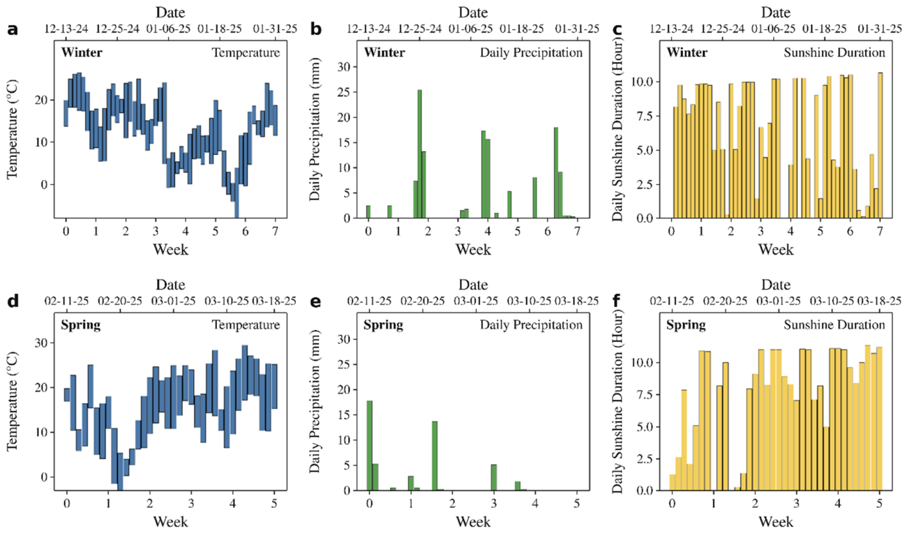
Figure 4 was constructed by aligning daily minimum-to-maximum temperature ranges, precipitation totals, and estimated sunshine duration for the winter (13 December 2024–31 January 2025; a–c) and spring (11 February–18 March 2025; d–f) weather windows. Calendar dates are shown above each panel and the corresponding weeks are shown below, with week 0 marking the first plotted date. Precipitation was compiled from National Weather Service CF6 reports for Sugar Land Regional Airport (KSGR) for December 2024 [58], January 2025 [59], February 2025 [60], and March 2025 [61], and converted from inches to millimeters; trace amounts were plotted as zero. During the winter experiment, the plotted temperature ranges fluctuated substantially and included freezing conditions in January, while estimated sunshine duration varied markedly among days (Figure 4a,c). Precipitation totaled approximately 130 mm over the longer 50-day window, including a daily maximum of 25.4 mm on December 25 (Figure 4b). The January 21 value of 8.1 mm includes the water equivalent of frozen precipitation [59]. This variable weather provides context for the winter nutrient response: TN removal was greatest in week 1 and comparatively high in week 3, TN concentrations rebounded in week 7, and TP concentrations were lower after the sampling gap (Figure 2). Cold conditions and variable light may have constrained outdoor plant activity, but the approximately three-week indoor period at about 25 °C under ceiling lights interrupted exposure to the outdoor weather. Because weeks 4 and 5 were excluded, nutrient changes during this interval cannot be resolved. The winter patterns therefore cannot be attributed to outdoor temperature, precipitation, or sunshine alone; indoor relocation and plant stress also limit the seasonal comparison.
Figure 4.
Weather conditions during winter (13 December 2024–31 January 2025) (a–c) and spring (11 February–18 March 2025) (d–f). Panels show daily minimum-to-maximum temperature ranges (a,d), precipitation (b,e), and estimated sunshine duration (c,f). Precipitation is from National Weather Service records for Sugar Land Regional Airport and includes snow water equivalent; trace amounts are plotted as zero [58,59,60,61]. Upper axes show calendar dates; lower axes show elapsed weeks from the first plotted date (week 0).
During our spring season’s experiment, a cold interval in February was followed by warmer conditions, with daily maxima often approximately 20–30 °C later in the record (Figure 4d). Estimated sunshine duration was variable early in the period and frequently approximately 7–11 h per day later (Figure 4f). Precipitation totaled approximately 48 mm over 36 days, with the largest events on February 11 (17.8 mm) and February 22 (13.7 mm), followed by fewer rainfall events (Figure 4e). The later warmer conditions and longer sunshine estimates are consistent with the larger TN and TP decreases observed after week 2, particularly for CR and TSB (Figure 3). Nutrient concentrations continued to decline during the less rainy part of the record. These observations provide a descriptive seasonal comparison; the separate contributions of temperature, light, and possible precipitation-related dilution were not quantified.
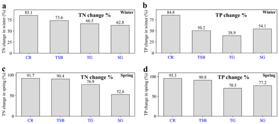
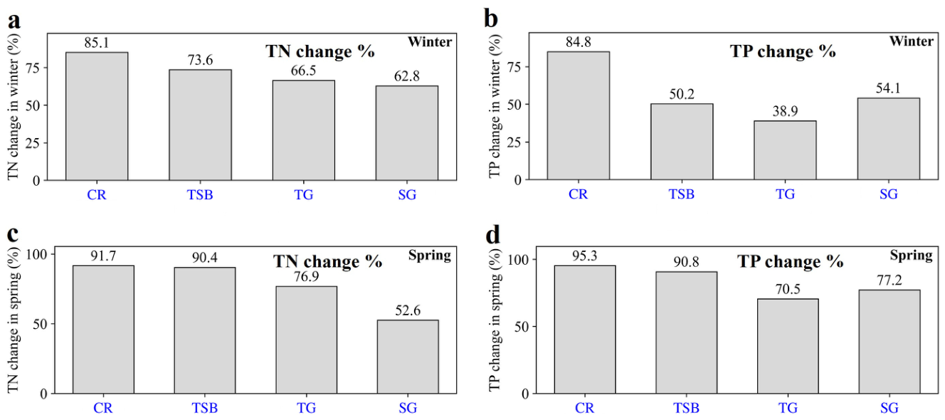
Figure 5 summarizes TN and TP removal efficiencies during winter and spring. CR achieved the highest winter TN and TP removals (85.1% and 84.8%, respectively; Figure 5a,b). Winter TN removal then ranked TSB (73.6%), TG (66.5%), and SG (62.8%), whereas winter TP removal ranked SG (54.1%), TSB (50.2%), and TG (38.9%). In spring, CR and TSB again showed the highest TN removals (91.7% and 90.4%) and TP removals (95.3% and 90.8%; Figure 5c,d). TG and SG had lower spring TN removals (76.9% and 52.6%) and TP removals (70.5% and 77.2%). Removal efficiencies were higher in spring for every species–nutrient combination except SG TN, which decreased from 62.8% to 52.6%. Thus, CR maintained the highest overall TN and TP removal efficiencies in both seasons, although the magnitude of the seasonal response varied among species.
Figure 5.
Total nitrogen (TN) and total phosphorus (TP) removal efficiencies (%) during winter (a,b) and spring (c,d). TN is shown in (a,c), and TP in (b,d). CR: common rush; TSB: three-square bulrush; TG: tiger grass; SG: switchgrass.
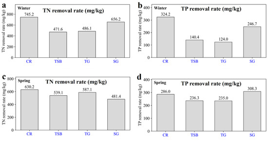
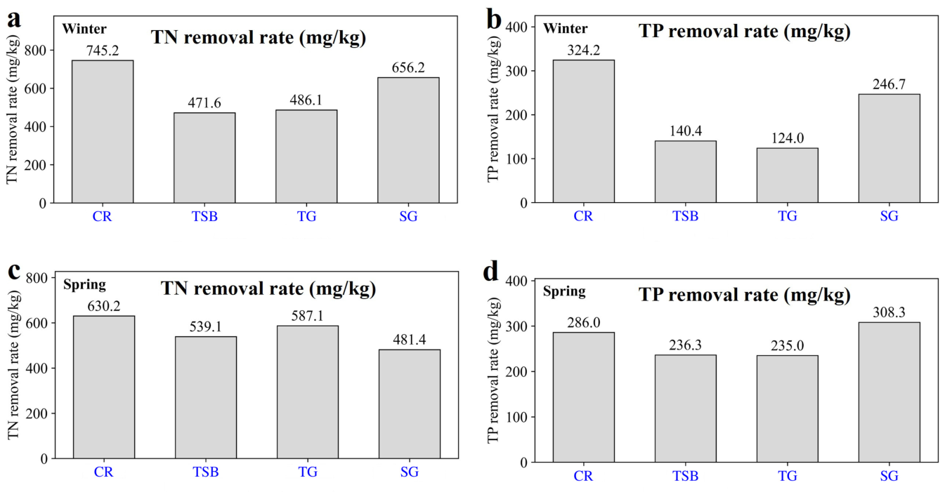
The fresh-weight-normalized values in Figure 6 provide descriptive comparisons of nutrient removal per unit plant biomass. In winter, CR showed the highest normalized TN and TP removal (745.2 and 324.2 mg kg−1, respectively), followed by SG (656.2 and 246.7 mg kg−1; Figure 6a,b). In spring, normalized TN removal ranked CR (630.2 mg kg−1) > TG (587.1 mg kg−1) > TSB (539.1 mg kg−1) > SG (481.4 mg kg−1), whereas normalized TP removal was highest for SG (308.3 mg kg−1), followed by CR (286.0 mg kg−1), TSB (236.3 mg kg−1), and TG (235.0 mg kg−1; Figure 6c,d). Seasonal changes therefore depended on both species and nutrient: normalized TN removal increased for TSB and TG but decreased for CR and SG, while normalized TP removal increased for TSB, TG, and SG but decreased for CR. These indices were calculated from the TN and TP results using the solution-volume correction described in Section 2.2.2 and Section 2.3.5.
Figure 6.
Fresh-weight-normalized total nitrogen (TN) and total phosphorus (TP) removal (mg kg−1) during winter (a,b) and spring (c,d). TN is shown in (a,c), and TP in (b,d). Values describe net nutrient removal per unit plant fresh biomass over each experimental period. CR: common rush; TSB: three-square bulrush; TG: tiger grass; SG: switchgrass.
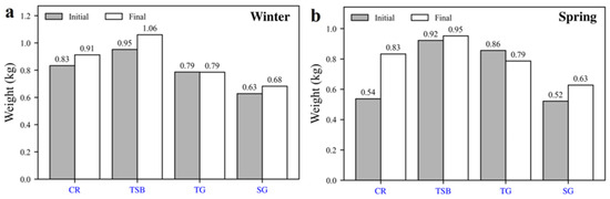
Figure 7 compares initial and final plant fresh weights. CR, TSB, and SG gained biomass in both displayed experiments, whereas TG remained unchanged in panel a and decreased by 0.07 kg in panel b. Positive fresh-weight changes ranged from 0.03 to 0.29 kg across species and experiments. These endpoint measurements illustrate species differences in biomass accumulation, but they do not resolve growth or senescence during the indoor interval. Fresh weight also reflects plant water content, so the normalized removal values should not be interpreted as direct measurements of intrinsic nutrient-uptake capacity.
Figure 7.
Initial and final plant fresh weights (kg) in (a) the winter experiment and (b) the spring experiment. Gray bars indicate initial weights and open bars indicate final weights. CR: common rush; TSB: three-square bulrush; TG: tiger grass; SG: switchgrass.
Together, the removal percentages and biomass-normalized values show that species rankings depend on the comparison used. CR performed strongly across both seasons, but higher spring removal percentages did not translate into uniform increases in removal per unit fresh biomass. Species selection should therefore consider total nutrient removal, standing biomass, and performance under variable seasonal conditions. The weather record provides environmental context for these comparisons without isolating the effects of individual meteorological variables.
3.5. Possible Mechanisms and Implications
Below, we discuss possible physiological mechanisms, based on previous studies, that may explain the seasonal differences in nutrient removal. Photosynthesis, enzyme activity, transporter kinetics, and root activity were not directly measured in this study.
These mechanisms may help explain the differences among seasons and plant species, but our experiments did not determine how much each mechanism contributed.
- Temperature control of physiology: Lower temperatures reduce enzyme activity, membrane transport, photosynthesis, and root respiration, collectively slowing nutrient assimilation and growth; warmer conditions may support plant growth and nutrient assimilation. These mechanisms may contribute to seasonal differences, but their effects were not measured separately here.
- Biomass versus intrinsic uptake: Absolute nutrient removal reflects both per-unit uptake capacity and standing biomass. Large biomass can yield high total removal even with modest per-kg uptake; normalizing by fresh biomass provides a descriptive comparison, subject to the measurement limitations noted above.
- Root and rhizosphere processes: Roots provide surface area for direct uptake and sustain root-zone oxygenation and microbial communities that mediate N and P transformations (mineralization, nitrification, microbial immobilization, sorption). Seasonal declines in root growth and exudation reduce these coupled plant–microbial pathways in winter, lowering system removal.
- Short-term dynamics and acclimation: Early concentration patterns may reflect acclimation and environmental conditions; transient P release (from root turnover or desorption) can produce initial stability or brief increases in TP before net removal resumes.
- Management implications: To support year-round FTW performance, prioritize species that combine high per-unit uptake and robust biomass production (e.g., CR), allow acclimation periods, and consider design strategies that moderate water temperature or increase residence time (longer hydraulic retention, mixed-species plantings, shallower basins or passive warming) to mitigate winter declines. Lightweight expanded clay aggregate (LECA) could also be a suitable support material and will be considered for testing in future studies.
4. Conclusions
This study compared seasonal TN and TP removal across four floating treatment wetland (FTW) species (CR, TSB, TG, and SG) using replicated 10 L bucket experiments with standardized initial loadings (60 mg L−1 TN, 26.5 mg L−1 TP). TN and TP concentrations, plant biomass, and growth metrics were monitored through winter and spring. Clear species- and season-dependent differences emerged: removal efficiencies were generally higher in spring than in winter, although SG showed lower TN removal in spring. CR performed best overall, achieving ~91.7% TN and 95.3% TP removal in spring, whereas SG showed lower removal. In spring, nutrient reductions were generally more pronounced after week 2, with early changes varying among species. Biomass-normalized values provided descriptive comparisons among species and seasons. These results indicate that FTWs can deliver effective seasonal nutrient reduction in southern climates and identify CR as a robust candidate for winter–spring nutrient management.
Supplementary Materials
The following supporting information can be downloaded at: https://www.mdpi.com/article/10.3390/environments13110633/s1, Figure S1: Juncus effusus (top left: in the wild; top right: in the small cup for floating test) and three-square bulrush (bottom left: in the wild; bottom right: in the small cup for floating test); Figure S2: (a) Three-square bulrush before (left) and after (right) soil removal. (b) Juncus effusus without soil; Figure S3: Juncus effusus (CR) growth images in different weeks; Figure S4: Three-square bulrush growth images in different weeks; Figure S5: Centella asiatica (TG) growth images in different weeks; Figure S6: Switchgrass growth images in different weeks; Figure S7: Regional outdoor air-temperature context for the winter experiment. Daily minimum and maximum air temperatures at Houston William P. Hobby Airport, Texas (NOAA GHCN-Daily station USW00012918), from 1 December 2024 to 31 January 2025. The dashed line marks 0 °C. The daily maximum for 24 January 2025 is omitted because it failed NOAA’s spatial consistency check; the gap was not interpolated. These airport observations provide regional context and are not measurements at the experimental site or in the buckets. The reported indoor air temperature during temporary protection was approximately 25 °C. The plotted values are provided in Table S3; Figure S8: Floating mat and tap water control experiment. (a) Ion concentration change after 3 weeks of soaking floating mat in the tap water. (b) Tap water ion concentration change after 3 weeks; Figure S9: Equipment and reagents for TN and TP analysis: GNST-900S Multi-Parameter Analyzer (a), GENESITE SJ-16X Rapid Digester (b), and TN and TP reagents (c); Table S1: Procedure to Measure Total Nitrogen with the GNST-900S; Table S2: Procedure to Measure Total Phosphorus with the GNST-900S; Table S3: Daily outdoor air temperatures at Houston William P. Hobby Airport (USW00012918), 1 December 2024–31 January 2025.
Author Contributions
V.B. and X.S. conceived the research idea, designed the experimental approach, and wrote the manuscript. L.P.S. and Y.C. conducted the experiments and collected the data. U.G. analyzed the data. W.Z. and R.L.R. provided technical suggestions and contributed to the refinement of the study. All authors have read and agreed to the published version of the manuscript.
Funding
X.S., V.B., and R.L.R. have received funding from the Environmental Protection Agency (EPA#02D48123). We also thank the University of Houston Center for Carbon Management and Energy (CCME) for supporting V.B. with a small research grant.
Data Availability Statement
Daily precipitation data used in Figure 4b,e are publicly available in National Weather Service CF6 reports for Sugar Land Regional Airport (KSGR; December 2024–March 2025) [58,59,60,61]. Regional daily air-temperature data used in Supplementary Figure S7 are provided in Supplementary Table S3 and are publicly available from NOAA GHCN-Daily (station USW00012918; https://doi.org/10.7289/V5D21VHZ) [51]. Experimental results are presented in the manuscript figures and Supporting Materials.
Acknowledgments
During the preparation of this manuscript, the authors used ChatGPT (OpenAI, GPT-6) solely for English-language polishing, including improvements to grammar, clarity, and readability. The authors have reviewed and edited the output and take full responsibility for the content of this publication. The authors gratefully acknowledge Bhupinder Singh for assisting with the transport of experimental containers and for maintaining the plants during the winter storm.
Conflicts of Interest
The authors declare no conflicts of interest.
Abbreviations
| FTW | Floating treatment wetlands |
| SG | Switchgrass |
| EPA | Environmental Protection Agency |
| TSB | Three-square bulrush |
| TG | Tiger Grass |
| CR | Common Rush |
| TP | Total phosphorus |
| TN | Total nitrogen |
References
- Peñuelas, J.; Sardans, J. The global nitrogen-phosphorus imbalance. Science 2022, 375, 266–267. [Google Scholar] [CrossRef] [Scilit] [PubMed]
- Zou, T.; Zhang, X.; Davidson, E.A. Global trends of cropland phosphorus use and sustainability challenges. Nature 2022, 611, 81–87. [Google Scholar] [CrossRef] [Scilit] [PubMed]
- Rabalais, N.N. Nitrogen in aquatic ecosystems. AMBIO J. Hum. Environ. 2002, 31, 102–112. [Google Scholar] [CrossRef] [PubMed]
- Smith, V.H.; Tilman, G.D.; Nekola, J.C. Eutrophication: Impacts of excess nutrient inputs on freshwater, marine, and terrestrial ecosystems. Environ. Pollut. 1999, 100, 179–196. [Google Scholar] [CrossRef] [Scilit] [PubMed]
- Lan, J.; Liu, P.; Hu, X.; Zhu, S. Harmful algal blooms in eutrophic marine environments: Causes, monitoring, and treatment. Water 2024, 16, 2525. [Google Scholar] [CrossRef] [Scilit]
- Tiwari, A.K.; Pal, D.B. Nutrients contamination and eutrophication in the river ecosystem. In Ecological Significance of River Ecosystems; Elsevier: Amsterdam, The Netherlands, 2022; pp. 203–216. [Google Scholar]
- Tariq, A.; Mushtaq, A. Untreated wastewater reasons and causes: A review of most affected areas and cities. Int. J. Chem. Biochem. Sci. 2023, 23, 121–143. [Google Scholar]
- Zahoor, I.; Mushtaq, A. Water pollution from agricultural activities: A critical global review. Int. J. Chem. Biochem. Sci. 2023, 23, 164–176. [Google Scholar]
- Devlin, M.; Brodie, J. Nutrients and eutrophication. In Marine Pollution–Monitoring, Management and Mitigation; Springer Nature: Cham, Switzerland, 2023; pp. 75–100. [Google Scholar]
- Oh, J.-W.; Shiv Charan Pushparaj, S.; Muthu, M.; Gopal, J. Review of harmful algal blooms (HABs) causing marine fish kills: Toxicity and mitigation. Plants 2023, 12, 3936. [Google Scholar] [CrossRef] [Scilit] [PubMed]
- Anderson, D.M.; Cembella, A.D.; Hallegraeff, G.M. Progress in understanding harmful algal blooms: Paradigm shifts and new technologies for research, monitoring, and management. Annu. Rev. Mar. Sci. 2012, 4, 143–176. [Google Scholar] [CrossRef] [Scilit] [PubMed]
- Wurtsbaugh, W.A.; Paerl, H.W.; Dodds, W.K. Nutrients, eutrophication and harmful algal blooms along the freshwater to marine continuum. Wiley Interdiscip. Rev. Water 2019, 6, e1373. [Google Scholar] [CrossRef] [Scilit]
- Shortle, J.S.; Mihelcic, J.R.; Zhang, Q.; Arabi, M. Nutrient control in water bodies: A systems approach. J. Environ. Qual. 2020, 49, 517–533. [Google Scholar] [CrossRef] [Scilit] [PubMed]
- Bănăduc, D.; Simić, V.; Cianfaglione, K.; Barinova, S.; Afanasyev, S.; Öktener, A.; McCall, G.; Simić, S.; Curtean-Bănăduc, A. Freshwater as a sustainable resource and generator of secondary resources in the 21st century: Stressors, threats, risks, management and protection strategies, and conservation approaches. Int. J. Environ. Res. Public Health 2022, 19, 16570. [Google Scholar] [CrossRef] [Scilit] [PubMed]
- Sitote, Y.M.; Gebremedhine, M.G. Comprehensive Review of Eutrophication in Freshwater Ecosystems: Causes, Effects, Assessment, and Management Strategies. Preprints 2024. [Google Scholar] [CrossRef] [Scilit]
- Wu, H.; Wang, R.; Yan, P.; Wu, S.; Chen, Z.; Zhao, Y.; Cheng, C.; Hu, Z.; Zhuang, L.; Guo, Z.; et al. Constructed wetlands for pollution control. Nat. Rev. Earth Environ. 2023, 4, 218–234. [Google Scholar] [CrossRef] [Scilit]
- David, G.; Rana, M.S.; Saxena, S.; Sharma, S.; Pant, D.; Prajapati, S.K. A review on design, operation, and maintenance of constructed wetlands for removal of nutrients and emerging contaminants. Int. J. Environ. Sci. Technol. 2023, 20, 9249–9270. [Google Scholar] [CrossRef] [Scilit]
- Muduli, M.; Choudharya, M.; Ray, S. A review on constructed wetlands for environmental and emerging contaminants removal from wastewater: Traditional and recent developments. Environ. Dev. Sustain. 2024, 26, 30181–30220. [Google Scholar] [CrossRef] [Scilit]
- Vymazal, J. Removal of nutrients in various types of constructed wetlands. Sci. Total Environ. 2007, 380, 48–65. [Google Scholar] [CrossRef] [Scilit] [PubMed]
- Brix, H. Wastewater treatment in constructed wetlands: System design, removal processes, and treatment performance. In Constructed Wetlands for Water Quality Improvement; CRC Press: Boca Raton, FL, USA, 2020; pp. 9–22. [Google Scholar]
- Wang, L.K.; Wang, M.-H.S.; Shammas, N.K.; Hahn, H.H. Physicochemical treatment consisting of chemical coagulation, precipitation, sedimentation, and flotation. In Integrated Natural Resources Research; Springer International Publishing: Cham, Switzerland, 2021; pp. 265–397. [Google Scholar]
- Wilfert, P.; Kumar, P.S.; Korving, L.; Witkamp, G.-J.; Van Loosdrecht, M.C. The relevance of phosphorus and iron chemistry to the recovery of phosphorus from wastewater: A review. Environ. Sci. Technol. 2015, 49, 9400–9414. [Google Scholar] [CrossRef] [Scilit] [PubMed]
- Nassef, E. Removal of phosphates from industrial waste water by chemical precipitation. Eng. Sci. Technol. An. Int. J. 2012, 2, 409–413. [Google Scholar]
- Peters, R.W.; White, T.E.; Ku, Y.; Engelder, C.L.; Anand, P.; Shedroff, S. Wastewater treatment: Physical and chemical methods. J. Water Pollut. Control Fed. 1986, 58, 481–490. [Google Scholar]
- Jaramillo, F.; Orchard, M.; Munoz, C.; Zamorano, M.; Antileo, C. Advanced strategies to improve nitrification process in sequencing batch reactors—A review. J. Environ. Manag. 2018, 218, 154–164. [Google Scholar] [CrossRef] [Scilit] [PubMed]
- Singh, M.; Srivastava, R.K. Sequencing batch reactor technology for biological wastewater treatment: A review. Asia-Pac. J. Chem. Eng. 2011, 6, 3–13. [Google Scholar] [CrossRef] [Scilit]
- Dutta, A.; Sarkar, S. Sequencing batch reactor for wastewater treatment: Recent advances. Curr. Pollut. Rep. 2015, 1, 177–190. [Google Scholar] [CrossRef] [Scilit]
- Sun, Y.; Guan, Y.; Pan, M.; Zhan, X.; Hu, Z.; Wu, G. Enhanced biological nitrogen removal and N2O emission characteristics of the intermittent aeration activated sludge process. Rev. Environ. Sci. Bio/Technol. 2017, 16, 761–780. [Google Scholar] [CrossRef] [Scilit]
- Sun, S.-P.; Nàcher, C.P.I.; Merkey, B.; Zhou, Q.; Xia, S.-Q.; Yang, D.-H.; Sun, J.-H.; Smets, B.F. Effective biological nitrogen removal treatment processes for domestic wastewaters with low C/N ratios: A review. Environ. Eng. Sci. 2010, 27, 111–126. [Google Scholar] [CrossRef] [Scilit]
- Justino, S.; Calheiros, C.S.; Castro, P.M.; Gonçalves, D. Constructed wetlands as nature-based solutions for wastewater treatment in the hospitality industry: A review. Hydrology 2023, 10, 153. [Google Scholar] [CrossRef] [Scilit]
- Bauer, L.H. Nature-Based Solutions: The Use of a Floating Wetland as an Alternative to Wastewater Treatment. Master’s Thesis, Universidade Federal do Rio Grande do Sul, Porto Alegre, Brazil, 2020. [Google Scholar]
- Pavlíková, M.; Odehnalová, K.; Zezulka, Š.; Maršálková, E.; Lamaczová, A.; Maršálek, B. Nature-Based Approaches for Managing Bioavailable Phosphorus in Aquatic Ecosystems. Hydrology 2025, 12, 236. [Google Scholar] [CrossRef] [Scilit]
- Rigotti, J.A.; Pasqualini, J.P.; Rodrigues, L.R. Nature-based solutions for managing the urban surface runoff: An application of a constructed floating wetland. Limnetica 2020, 39, 441–454. [Google Scholar] [CrossRef] [Scilit]
- Paranychianakis, N.V.; Angelakis, A.N.; Leverenz, H.; Tchobanoglous, G. Treatment of wastewater with slow rate systems: A review of treatment processes and plant functions. Crit. Rev. Environ. Sci. Technol. 2006, 36, 187–259. [Google Scholar] [CrossRef] [Scilit]
- Wu, H.; Zhang, J.; Hao Ngo, H.; Guo, W.; Hu, Z.; Liang, S.; Fan, J.; Liu, H. A review on the sustainability of constructed wetlands for wastewater treatment: Design and operation. Bioresour. Technol. 2015, 175, 594–601. [Google Scholar] [CrossRef] [Scilit] [PubMed]
- Shen, S.; Li, X.; Lu, X. Recent developments and applications of floating treatment wetlands for treating different source waters: A review. Environ. Sci. Pollut. Res. 2021, 28, 62061–62084. [Google Scholar] [CrossRef] [Scilit] [PubMed]
- Bista, S.; Karki, B.K.; Maharjan, R. A Review Paper on Floating Treatment Wetlands: Working Principles and Applications for River Water Remediation. J. Adv. Coll. Eng. Manag. 2025, 10, 13–30. [Google Scholar] [CrossRef] [Scilit]
- Sahreen, S.; Mukhtar, H. Floating Treatment Wetlands (FTW) for Sustainable Industrial Treatment. Microb. Bioremediation Multiomics Technol. Sustain. Dev. Recent Trends 2024, 13, 291. [Google Scholar] [CrossRef] [Scilit]
- Gao, T.; Li, Y.; Yang, N.; Xiong, W.; Liang, X.; Wang, Y. Plant-rhizosphere microbe interactions and their roles in nitrogen cycles under periodic flooding: From cooperation mechanisms to ecological responses. Crit. Rev. Environ. Sci. Technol. 2025, 55, 1358–1382. [Google Scholar] [CrossRef] [Scilit]
- Fang, J.; Zhao, R.; Cao, Q.; Quan, Q.; Sun, R.; Liu, J. Effects of emergent aquatic plants on nitrogen transformation processes and related microorganisms in a constructed wetland in northern China. Plant Soil 2019, 443, 473–492. [Google Scholar] [CrossRef] [Scilit]
- Richardson, A.E.; Barea, J.-M.; McNeill, A.M.; Prigent-Combaret, C. Acquisition of phosphorus and nitrogen in the rhizosphere and plant growth promotion by microorganisms. Plant Soil 2009, 321, 305–339. [Google Scholar] [CrossRef] [Scilit]
- Afzal, M.; Arslan, M.; Müller, J.A.; Shabir, G.; Islam, E.; Tahseen, R.; Anwar-ul-Haq, M.; Hashmat, A.J.; Iqbal, S.; Khan, Q.M. Floating treatment wetlands as a suitable option for large-scale wastewater treatment. Nat. Sustain. 2019, 2, 863–871. [Google Scholar] [CrossRef] [Scilit]
- Headley, T.; Tanner, C.C.; Auckland Regional Council. Application of Floating Wetlands for Enhanced Stormwater Treatment: A Review; Auckland Regional Council: Auckland, New Zealand, 2008. [Google Scholar]
- Stefanakis, A.I. The role of constructed wetlands as green infrastructure for sustainable urban water management. Sustainability 2019, 11, 6981. [Google Scholar] [CrossRef] [Scilit]
- Sangamnere, R.; Misra, T.; Bherwani, H.; Kapley, A.; Kumar, R. A critical review of conventional and emerging wastewater treatment technologies. Sustain. Water Resour. Manag. 2023, 9, 58. [Google Scholar] [CrossRef] [Scilit]
- Majsztrik, J.C.; Fernandez, R.T.; Fisher, P.R.; Hitchcock, D.R.; Lea-Cox, J.; Owen, J.S., Jr.; Oki, L.R.; White, S.A. Water use and treatment in container-grown specialty crop production: A review. Water Air Soil Pollut. 2017, 228, 151. [Google Scholar] [CrossRef] [Scilit] [PubMed]
- Li, J.; Qiu, Y.; Tian, Y.; Liu, Y.; Liu, G.; Feng, Y. Large-scale carbon nanotube-modified anodes enhance interfacial electron transfer and pollutant removal in field-scale ecological floating bed microbial electrochemical systems. Resour. Environ. Sustain. 2026, 27, 100376. [Google Scholar] [CrossRef] [Scilit]
- Uline. Plastic Pail with Lid—5 Gallon, S-14960. Product Specifications. Available online: https://www.uline.com/Product/Detail/S-14960/Hazardous-Materials-Packaging/Plastic-Pail-with-Lid-5-Gallon (accessed on 21 October 2026).
- GENESITE Environmental Protection Technology Co., Ltd. Can Activated Carbon be Used to Remove COD from Wastewater? GNST-900S Determination Principles. 23 October 2024. Available online: https://en.genesit1.com/Blog_details/62.html (accessed on 17 October 2026).
- GB/T 11893-1989; Water Quality—Determination of Total Phosphorus—Ammonium Molybdate Spectrophotometric Method. State Bureau of Technical Supervision: Beijing, China, 1989. Available online: https://openstd.samr.gov.cn/bzgk/std/newGbInfo?hcno=E3834D3D19D975F69C69CB359BCB762E (accessed on 17 October 2026).
- Menne, M.J.; Durre, I.; Korzeniewski, B.; McNeill, S.; Thomas, K.; Yin, X.; Anthony, S.; Ray, R.; Vose, R.S.; Gleason, B.E.; et al. Global Historical Climatology Network–Daily (GHCN-Daily), Version 3.35; NOAA National Climatic Data Center: Asheville, NC, USA, 2012. [Google Scholar] [CrossRef] [Scilit]
- Wei, Y.; Zhang, M.; Cui, L.; Pan, X.; Liu, W.; Li, W.; Lei, Y. Winter Decomposition of Emergent Macrophytes Affects Water Quality under Ice in a Temperate Shallow Lake. Water 2020, 12, 2640. [Google Scholar] [CrossRef] [Scilit]
- Dekle, J.; Strosnider, W.H.J.; White, S.A. Phosphorus uptake and release patterns in overwintering constructed floating wetlands. Water Sci. Technol. 2024, 89, 588–602. [Google Scholar] [CrossRef] [Scilit] [PubMed]
- Gordon, L.I.; Jennings, J.C., Jr.; Ross, A.A.; Krest, J.M. A Suggested Protocol for Continuous Flow Automated Analysis of Seawater Nutrients (Phosphate, Nitrate, Nitrite and Silicic Acid) in the WOCE Hydrographic Program and the Joint Global Ocean Fluxes Study. OSU Technical Report 93-1. 1993. Available online: https://www.nodc.noaa.gov/archive/arc0001/9900162/2.2/data/0-data/jgofscd/Files/protocols/Chap8.htm (accessed on 4 November 2026).
- Khan, T.F.; Hodson, M.E. Polyethylene microplastic can adsorb phosphate but is unlikely to limit its availability in soil. Heliyon 2024, 10, e23179. [Google Scholar] [CrossRef] [Scilit] [PubMed]
- Shen, S.; Geng, Z.; Li, X.; Lu, X. Evaluation of phosphorus removal in floating treatment wetlands: New insights in non-reactive phosphorus. Sci. Total Environ. 2022, 815, 152896. [Google Scholar] [CrossRef] [Scilit] [PubMed]
- Xu, B.; Wang, X.; Liu, J.; Wu, J.; Zhao, Y.; Cao, W. Improving Urban Stormwater Runoff Quality by Nutrient Removal through Floating Treatment Wetlands and Vegetation Harvest. Sci. Rep. 2017, 7, 7000. [Google Scholar] [CrossRef] [Scilit] [PubMed]
- National Weather Service. Preliminary Local Climatological Data (WS Form F-6), Sugar Land/Hull Field (CF6SGR), December 2024. NOAA/NWS Houston/Galveston, 1 January 2025. Available online: https://mesonet.agron.iastate.edu/wx/afos/p.php?e=202501011510&pil=CF6SGR (accessed on 4 November 2026).
- National Weather Service. Preliminary Local Climatological Data (WS Form F-6), Sugar Land/Hull Field (CF6SGR), January 2025. NOAA/NWS Houston/Galveston, 1 February 2025. Available online: https://mesonet.agron.iastate.edu/wx/afos/p.php?e=202502011510&pil=CF6SGR (accessed on 4 November 2026).
- National Weather Service. Preliminary Local Climatological Data (WS Form F-6), Sugar Land/Hull Field (CF6SGR), February 2025. NOAA/NWS Houston/Galveston, 1 March 2025. Available online: https://mesonet.agron.iastate.edu/wx/afos/p.php?e=202503011510&pil=CF6SGR (accessed on 4 November 2026).
- National Weather Service. Preliminary Local Climatological Data (WS Form F-6), Sugar Land/Hull Field (CF6SGR), March 2025. NOAA/NWS Houston/Galveston, 1 April 2025. Available online: https://mesonet.agron.iastate.edu/wx/afos/p.php?e=202504011410&pil=CF6SGR (accessed on 4 November 2026).
Disclaimer/Publisher’s Note: The statements, opinions and data contained in all publications are solely those of the individual author(s) and contributor(s) and not of MDPI and/or the editor(s). MDPI and/or the editor(s) disclaim responsibility for any injury to people or property resulting from any ideas, methods, instructions or products referred to in the content. |
© 2026 by the authors. Licensee MDPI, Basel, Switzerland. This article is an open access article distributed under the terms and conditions of the Creative Commons Attribution (CC BY) license.