Global Medium-Term Earthquake Forecasting with Every Earthquake a Precursor According to Scale

Abstract

The “Every Earthquake a Precursor According to Scale” (EEPAS) model uses minor earthquakes in a catalogue to forecast major earthquakes, based on the precursory scale increase phenomenon and associated predictive scaling relations. It has previously been applied to regional earthquake catalogues for medium-term forecasting of earthquakes with target magnitudes exceeding thresholds in the range M 5.0–6.0 using previous earthquakes about two magnitude units below the target threshold, depending on the completeness of the catalogue. Here, we apply it to the ISC-GEM global earthquake catalogue and test its ability to forecast earthquakes with target magnitudes exceeding M 7.5, i.e., the largest and most important earthquakes for assessing earthquake hazard. We use background models based on both smoothed seismicity and spatial variation of strain rate estimates. The models are fitted to the period 1994–2013, with 85 target earthquakes, and tested on the period 2014–2019, with 19 target earthquakes. The EEPAS model shows larger information gains over a smoothed seismicity model than in most regional applications. Also, a hybrid composed of EEPAS, smoothed seismicity and the strain rate outperforms a hybrid consisting only of smoothed seismicity and strain rate components. These preliminary results suggest that EEPAS may be useful for forecasting the largest earthquakes globally but should be followed up by transparent prospective testing. There are several avenues for improvement of EEPAS modeling.

1. Introduction

The largest earthquakes in the world can cause both widespread strong shaking and serious induced perils, such as landslides and tsunamis. Learning how to forecast them is important for understanding the time variation of seismic hazard and risk and is key for enhancing earthquake preparedness and countermeasure planning.

Improved forecasting of large earthquakes is not easily achieved. There is no known single observation that can be used to forecast the occurrence of a large earthquake within narrow time and space limits with high probability. Therefore, earthquake forecasting exists in a low-probability environment [1]. However, the last three decades have seen progress in the development of synoptic forecasting models, which estimate the expected earthquake occurrence as a function of time, magnitude and location within a region of surveillance. This progress has been encouraged by prospective testing experiments of the Collaboratory for the Study of Earthquake Predictability (CSEP) [2,3]. Some models have already proved useful for public earthquake forecasting and in hazard and risk applications. The overriding scientific goal is that, with further development of individual models, the formation of hybrids and the inclusion of new and improved data inputs, the information gains will progressively accumulate to increase the usefulness of the best forecasting models on all timescales. This is the “brick by brick” approach to earthquake forecasting enunciated by Jordan [1]. Here, we describe a small step towards achieving the overriding goal.

Earthquake forecasting models can be grouped by timescale into short-term, medium-term and long-term models [4]. Short-term models typically have a time horizon ranging from hours to months. They most commonly aim to capture the temporal and spatial variation of seismicity associated with short-term clustering, including the phenomena of foreshocks, mainshocks and aftershocks. Well-known models in this class are the Epidemic Type Aftershock model [5] and the Short-Term Earthquake Probability model [6]. Some models including non-seismic precursory phenomena and physics-based modelling also belong to this class [7,8]. Long-term models typically have a time horizon of decades to millennia. These models are commonly applied for probabilistic seismic hazard analysis [9] and aim to estimate the spatial variation of the long-term average rate of earthquake occurrence in a region, usually based on expected recurrence of ruptures on known faults and/or spatial smoothing of the locations of past earthquakes [10,11]. Medium-term forecasting models cover the gap between these two classes by offering a time horizon ranging from months to decades. A well-studied model in this class is the “Every Earthquake a Precursor According to Scale” (EEPAS) model [12]. It aims to capture temporal and spatial variation of seismicity associated with medium-term clustering.

The EEPAS model provides the medium-term component of practical earthquake forecasts issued following major earthquakes in New Zealand since 2011 [13]. It has previously been fitted to and tested on other regional catalogues, but not to a global catalogue [12,14,15,16]. EEPAS has been included in regional CSEP testing in California, New Zealand and Japan [17,18,19]. Here, we scope its potential for global forecasting by fitting it to a global catalogue, with a view to submitting it for future transparent testing and to planning technical elaborations of the model to improve its forecasting performance.

The availability of a homogeneous earthquake catalogue with a low magnitude of completeness over a long period is necessary for developing dependable forecasting models. An advantage of global catalogues is that they contain frequent large earthquakes to test forecasting models against. Regional earthquake forecasting experiments have tended to adopt low target magnitude thresholds (e.g., M5.0 for medium- and long-term models, and M4.0 for short-term models) to obtain statistically significant results within a testing period of a few years. However, with such low thresholds, not all target earthquakes contribute significantly to hazard and risk. A disadvantage of global catalogues is their lack of completeness at low magnitudes; the smaller events play an important role in forecasting the larger earthquakes in EEPAS. Careful choice of input and target magnitude thresholds is needed to obtain sufficient completeness at lower magnitudes to support fitting of a global EEPAS model.

The EEPAS model is usually fitted with the Proximity to Past Earthquake (PPE) smoothed seismicity model as background. The PPE model has a rate density that varies continuously in space and time. Here, as an alternative and additional background model, we consider a gridded earthquake likelihood model based on a global strain rate model [20]. This is a natural step because strain rates and earthquakes are physically linked, and it has already been shown that combining strain rates with smoothed seismicity produces improved earthquake likelihood models [21,22]. The strain rate model is derived from Global Navigation Satellite System (GNSS) data over the period 1990–2013 and does not incorporate time variation.

2. Materials and Methods

2.1. Precursory Scale Increase and the EEPAS Model

The precursory scale increase (Ψ) phenomenon [23] is an increase in the rate of occurrence and magnitude of minor earthquakes observed to occur in the medium term before the occurrence of major earthquakes in well-catalogued regions. The medium term here ranges from months to decades, depending on the magnitude of the major earthquake (mainshock). Each identification of Ψ is associated with a mainshock magnitude $M_m$, a precursor magnitude $M_P$, a precursor time $T_P$ and a precursory area $A_P$ that encompasses the precursory earthquakes, mainshock and aftershocks. $T_P$ is the time between the onset of precursory seismicity and the occurrence of the mainshock, and $M_P$ is the average of the three largest precursory earthquake magnitudes.

The EEPAS model is based on three empirical predictive scaling relations derived by Evison and Rhoades [23] using 47 identifications of Ψ from the catalogues of Japan, California and northern Mexico, Greece and northwest Türkiye, and New Zealand. Further examples of Ψ have been identified in Australia and in synthetic earthquake catalogues generated by physics-based earthquake simulators [24,25]. The predictive relations for $M_m$, $T_P$ and $A_P$, given $M_P$, are:

$$M_m=a_M+b_M{M}_P; \log T_P=a_T+b_T{M}_P; \mathrm{and} \log A_P=a_A+b_A{M}_P,$$

(1)

where $a_M$, $b_M,$ $a_T, b_T$, $a_A$ and $b_A$ are linear regression parameters.

The EEPAS model [12] is not aimed at identifying the Ψ-phenomenon. Instead, it regards every earthquake as a precursor of larger events expected to follow it in the medium term. Taking its magnitude as an instance of $M_P$, it uses the Ψ predictive relations to forecast the distribution of the time of occurrence t, magnitude m and location $\left(x,y\right)$ of the expected following events. For a precursory earthquake at time $t_i$, with magnitude m_i and location ($x_i,y_i$), the associated probability densities take the form

$$f\left(t|t_i,m_i\right)={\displaystyle \frac{H\left(t-t_i-l\right)}{\left(t-t_i\right){\mathsf{\sigma }}_T\ln \left(10\right)\sqrt{2\pi }}} exp\left[-{\displaystyle \frac{1}{2}}\left({\displaystyle \frac{\log \left(t-t_i\right)-a_T-b_T{m}_i}{{\mathsf{\sigma }}_T}}\right)\right],$$

(2)

where l is a time lag between the time of occurrence of an earthquake and its inclusion in the model, H(s) = 1 if s > 0 and zero otherwise, and $a_T$, $b_T$ and ${\mathsf{\sigma }}_T$ are time parameters;

$$g\left(m|m_i\right)={\displaystyle \frac{1}{{\mathsf{\sigma }}_M\sqrt{2\pi }}}\exp \left[-{{\displaystyle \frac{1}{2}}\left({\displaystyle \frac{m-a_M-b_M{m}_i}{{\mathsf{\sigma }}_M}}\right)}^2\right],$$

(3)

where $a_M$, $b_M$ and ${\mathsf{\sigma }}_M$ are magnitude parameters; and

$$h\left(x,y|x_i,y_i,m_i\right)={\displaystyle \frac{1}{2\pi {\mathsf{\sigma }}_A^2{10}^{b_A{m}_i}}}\exp \left[-{\displaystyle \frac{{(x-x_i)}^2+{(y-y_i)}^2}{2{\mathsf{\sigma }}_A^2{10}^{b_A{m}_i}}}\right],$$

(4)

where $b_A$ and ${\mathsf{\sigma }}_A$ are area parameters. Equation (2) is based on the predictive relation for $T_P$, assuming a lognormal distribution for the time of occurrence. Equation (3) is based on the predictive relation for $M_m$, assuming a normal distribution for magnitude. Equation (4) is based on the predictive relation for $A_P$, assuming a circular bivariate normal distribution for location. There is an obvious connection between the parameters $a_M$,${ b}_M,a_T$, $b_T$ and $b_A$ in the EEPAS model and the parameters of the same name in Equation (1), but the EEPAS parameters are fitted independently of the Ψ scaling relations.

The contribution of the ith precursory earthquake to the EEPAS model rate density is given by

$${\lambda }_i\left(t,m,x,y\right)=w_{i}f\left(t|t_i,m_i\right)g\left(m|m_i\right)h\left(x,y|x_i,y_i,m_i\right).$$

(5)

where $w_i$ is a weighting factor that allows some precursory earthquakes to be more highly weighted than others.

The time-varying component of the EEPAS model is a normalized sum of the contributions from all precursory earthquakes with a magnitude not less than a threshold of completeness $m_0$ and time of occurrence $t_i$ not less than a starting time $t_0$:

$${\lambda }_{\mathrm{E}\mathrm{E}\mathrm{P}\mathrm{T}\mathrm{V}}\left(t,m,x,y\right)=\sum _{t_i\ge t_0,m_i\ge m_0}{\displaystyle \frac{\eta \left(m_i\right){\lambda }_i\left(t,m,x,y\right)}{\mathsf{\Delta }\left(m\right)}} ,$$

(6)

where $t_0$ is the starting time of the earthquake catalogue, η is a normalizing function and $1/\mathsf{\Delta }\left(m\right)$ compensates for missing contributions from precursory earthquakes with magnitudes less than $m_0$, which are not in the input catalogue. Here,

$$\mathsf{\Delta }\left(m\right)=\mathsf{\Phi }\left({\displaystyle \frac{m-a_M-b_M{m}_0-{\mathsf{\sigma }}_M^2\beta }{{\mathsf{\sigma }}_M}}\right),$$

(7)

where $\beta =b_{EEP}\ln 10$ and $b_{\mathrm{E}\mathrm{E}\mathrm{P}}$ is the Gutenberg–Richter b-value [26] that best relates the number of input earthquakes to the number of target earthquakes.

The rate density ${\lambda }_{\mathrm{E}\mathrm{E}\mathrm{P}\mathrm{T}\mathrm{V}}$ is defined for target magnitudes $m$ above a magnitude cutoff $m_c$ and for epicentral locations $(x,y)$ within a region of surveillance R. Typically, $m_c$ is chosen to be about 2 units larger than $m_0$ to ensure satisfactory completeness of the precursory earthquake contributions for all target magnitudes. Allowing for multiple background models, the EEPAS model forecasts the rate density through a convex linear combination of ${\lambda }_{\mathrm{E}\mathrm{E}\mathrm{P}\mathrm{T}\mathrm{V}}$ with $n_B$ background rate densities $\left\{{\lambda }_{Bi}, i=1,n_B\right\}:$

$${\lambda }_{\mathrm{E}\mathrm{E}\mathrm{P}\mathrm{A}\mathrm{S}}\left(t,m,x,y\right)={\displaystyle \sum _{i=1}^{n_B}}{{\mu }_{Bi}\lambda }_{Bi}\left(t,m,x,y\right)+{\lambda }_{\mathrm{E}\mathrm{E}\mathrm{P}\mathrm{T}\mathrm{V}}\left(t,m,x,y\right),$$

(8)

where ${\mu }_{Bi}$ is the proportional contribution of ${\lambda }_{Bi}$ to the mixture. If $\mu ={\sum }_{i=1}^{n_B}{\mu }_{Bi}$, then the proportional contribution ${\mu }_{EEPTV}$ of ${\lambda }_{\mathrm{E}\mathrm{E}\mathrm{P}\mathrm{T}\mathrm{V}}$ to the mixture is $1-\mu$. This contribution is accounted for in the normalizing function η, defined for a given magnitude v by

$$\eta (v)={\displaystyle \frac{b_M(1-\mu )}{E\left(w\right)}}\exp \left[-\beta \left(a_M+\left(b_M-1\right)v+{\displaystyle \frac{{\mathsf{\sigma }}_M^2\beta }{2}}\right)\right],$$

(9)

where β is related to the b-value as in Equation (7) and E(w) is the mean weight of earthquakes above the input magnitude threshold $m_0$. The normalizing function ensures that in the long run the forecasted earthquakes and the earthquakes in the catalogue have similar average rates of occurrence and magnitude distributions [12].

2.2. PPE Model

EEPAS has usually been applied with a single smoothed seismicity background model based on proximity to the epicenters of past earthquakes (PPE) [12,27]. The PPE model has rate density

$${\lambda }_{\mathrm{P}\mathrm{P}\mathrm{E}}\left(t,m,x,y\right)={\displaystyle \frac{\beta \mathrm{e}\mathrm{x}\mathrm{p}\left[-\beta (m-m_c)\right]}{t-t_0}}\sum _{m_{i\ge }{m}_c;t_0\le t_i<t}\left[a\left(m_i-m_c\right){\displaystyle \frac{1 }{\pi }}\left({\displaystyle \frac{1}{d^2+r_i^2}}\right)+s\right]$$

(10)

where $\beta$ is as in (7); $r_i$ is the distance in km between $(x,y)$ and $(x_i,y_i)$; $a$ is a normalization constant; $d$ is a smoothing distance parameter; and $s$ is a small constant to allow for earthquakes occurring far from past earthquakes. The likelihood calculation for the PPE model has a component that depends on integrating the rate density over the time, region of surveillance and magnitude range of the target sets of earthquakes used for fitting and testing. In previous regional modeling, this integration was performed using great-circle distances between points but with an otherwise flat-Earth approximation of the Earth’s surface. Such an approximation has sufficient accuracy if the maximum distance between any two points in the region of surveillance is only a small fraction of the circumference of the Earth. In the global model, it is necessary to take the finite area and curvature of the Earth’s surface into account when performing this integration.

2.3. ISC-GEM Earthquake Catalogue

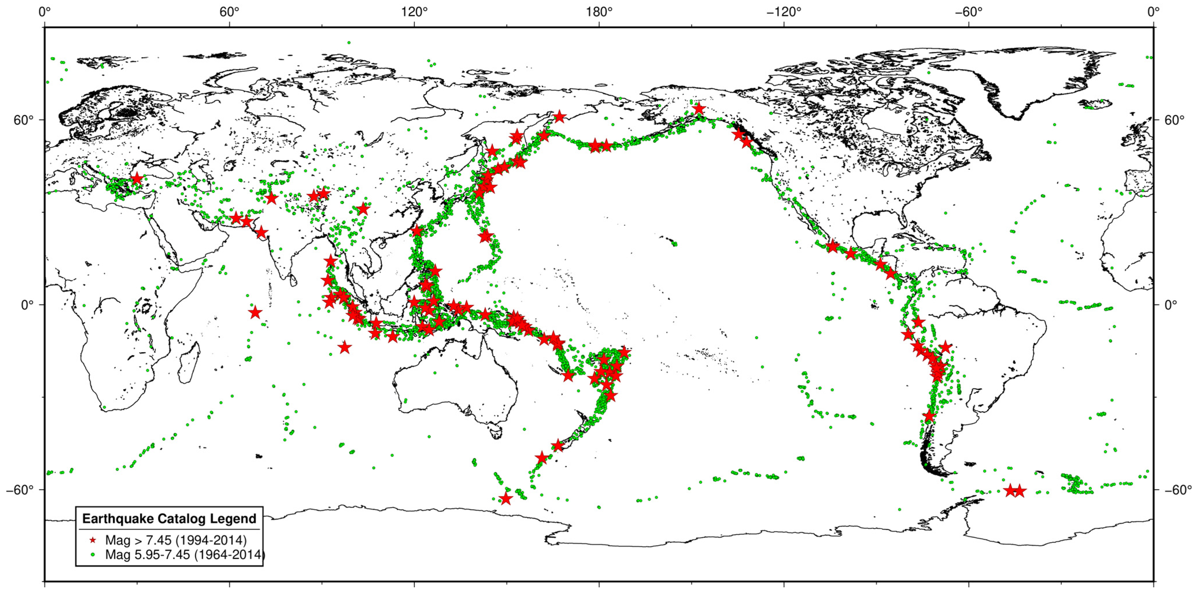
The ISC-GEM earthquake catalogue, developed by the International Seismological Centre (ISC) and the Global Earthquake Model (GEM) project, is a global catalogue beginning in 1900 [28]. Version 10.0 of the catalogue, which is used here, covers the period 1900–2019. The catalogue is considered complete for magnitude 6 and above from 1964 on [29]. Accordingly, the input data for this study is restricted to earthquakes with magnitude M ≥ 5.95 and depth ≤ 40 km from 1964–2019. The aim is to forecast target earthquakes with magnitude M ≥ 7.45. For the purposes of model fitting and testing, this period is divided into a warm-up period from 1964 to 1993 to accommodate the precursors to target earthquakes, a fitting period from 1994 to 2013 with 85 target earthquakes, and a testing period from 2014 to 2019 with 19 target earthquakes. Figure 1 shows the locations of relevant earthquake subsets in the ISC-GEM catalogue.

Figure 1. Earthquakes with magnitude $M\ge 5.95 \mathrm{a}\mathrm{n}\mathrm{d} \mathrm{d}\mathrm{e}\mathrm{p}\mathrm{t}\mathrm{h}\le 40 \mathrm{k}\mathrm{m}$ in the ISC-GEM catalogue in the period 1964–2013 (green dots) and target earthquakes with magnitudes $M\ge 7.45$ in the fitting period 1994–2013 (red stars).

2.4. GSR Model

We use the second invariant of the global strain rate model (GSRM v2.2) by Kreemer et al. [20]. GSRM v2.2 was derived from more than 24,000 velocity observations using GNSS data from the period 1990–2013. GSRM v2.2 has been used in the Global Earthquake Activity Rate (GEAR1) model for global shallow earthquakes with magnitude M ≥ 6 [21].

The gridded strain rates are defined in cells 0.1 degrees in latitude and longitude between longitudes 87.5° N and 87.5° S. This restricts the region of surveillance R for all models in our study to be the entire globe except for the polar regions with latitudes greater than 87.5°. The gridded strain rates are zero in many cells. We convert these rates into a time-invariant global strain rate (GSR) earthquake likelihood model [30,31] for magnitudes M ≥ 7.45, which is fitted to the period from 1994 to 2013. A multiplicative modeling technique [32] is used for the conversion. We start with a simple baseline model—the Stationary Uniform Poisson (SUP) likelihood model defined on the same grid. SUP is time-invariant and is based on a spatially uniform earthquake occurrence rate density and an exponential magnitude distribution discretized into bins of width 0.1 units. SUP has two parameters, a Gutenberg–Richter b-value and a normalization parameter that matches the total expected number of target earthquakes to the observed number. These were both fitted to the period 1994–2013. The multiplicative modeling method creates a multiplicative hybrid of SUP and the strain rate model.

$${\mathsf{\Gamma }}_{\mathrm{G}\mathrm{S}\mathrm{R}}\left(j,k\right)={\mathsf{\Gamma }}_{\mathrm{S}\mathrm{U}\mathrm{P}}\left(j.k\right)\exp \left(a\right)f_i\left[\rho \left(j\right)\right],$$

(11)

where $\rho \left(j\right)$ denotes the strain rate in a spatial cell j, $\mathsf{\Gamma }(j,k)$ denotes the expected number of earthquakes in a spatial cell j and magnitude bin k of a gridded earthquake likelihood model over a period of T days, and $f_i$ is an order-preserving function of the form

$$f_i\left(\rho \right)={b\left[\log \left(1+\rho \right)\right]}^c.$$

(12)

The parameters a, b and c are fitted to optimize the log-likelihood of the GSR model, given by

$$\ln L_{GSR}={\displaystyle \sum _{n=1}^N}\ln {\mathsf{\Gamma }}_{GSR}(j_n,k_n)-{\widehat{N}}_{GSR},$$

(13)

where there are N target earthquakes in cells and bins $\left\{\left(j_n,k_n\right), n=1\dots .,N\right\},$ and ${\widehat{N}}_{GSR}$ denotes the total expected number of target earthquakes, i.e., the sum of all the cell and bin rates in the model. The discrete Poisson likelihood [31] has an additional term involving the factorial of the observed number of events in each cell and bin. We ignore that term here because it does not affect either the maximum likelihood estimation of parameters or the information gain of one model over another [33].

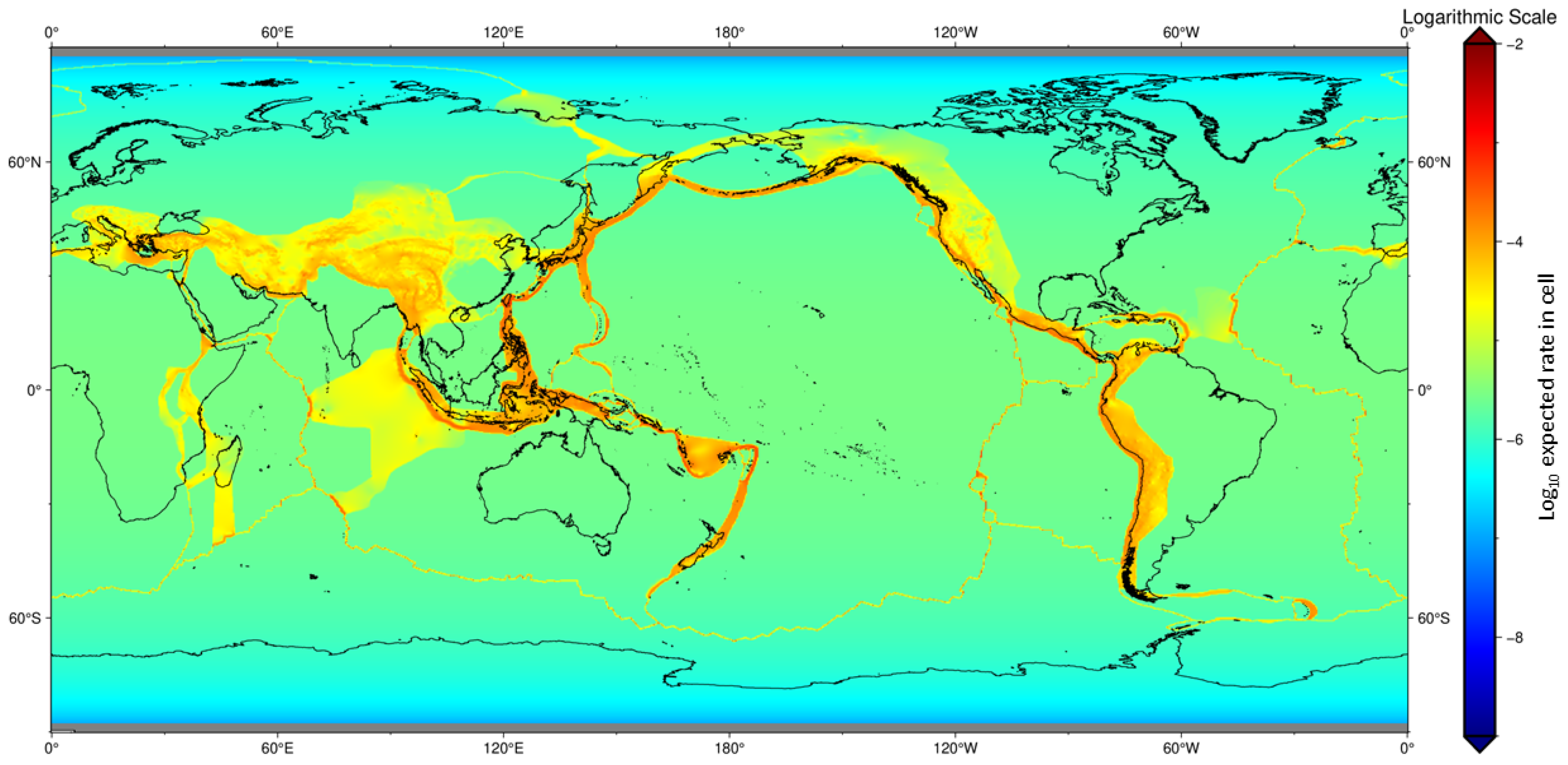
The GSR likelihood model does not have a zero expected number of earthquakes in any cell and bin pair. The magnitude distribution in the GSR model is inherited from that of the baseline SUP model, which, considering the Gutenberg–Richter relation, is assumed to be exponential. The spatial distribution of the GSR model’s expected number of target earthquakes per cell is displayed in Figure 2.

Figure 2. Spatial distribution of the logarithm of the expected number of earthquakes with magnitude $M\ge 7.45$ in cells of the GSR likelihood model fitted to the ISC-GEM catalogue over the period 1964–2013.

When mixing a gridded likelihood model $\mathsf{\Gamma }$ with a continuous model such as EEPAS or PPE, it is necessary to reconcile the gridded rates of the likelihood model with the rate densities of the continuous model. For this purpose, we regard the rate density of the gridded model as being constant within each spatial cell and exponentially distributed in magnitude. The rate density of a gridded likelihood model is thus given by

$$\lambda \left(t,m,x,y\right)={\displaystyle \frac{\mathsf{\Gamma }\left(j_{x,y},k_m\right)\beta \mathrm{e}\mathrm{x}\mathrm{p}(-\beta m)}{A_{j_{x,y}}T\left[\exp \left(-\beta m_{min}\left(k_m\right)\right)-\exp \left(-\beta m_{max}\left(k_m\right)\right)\right]}},$$

(14)

where $\beta$ is defined as in Equation (7), $j_{x,y}$ is the spatial cell containing $(x,y)$ and $A_{j_{x,y}}$ is its area, in km²; and $k_m$ is the magnitude bin containing $m$ with lower and upper limits $m_{min}\left(k_m\right)$ and $m_{max}\left(k_m\right),$ respectively.

3. Results

3.1. Fitting

Eight different global models were fitted to optimize their performance in forecasting target earthquakes in the period 1994–2013. These are the SUP model, the PPE model, the GSR model, a mixture of these two (GSR-PPE) and EEPAS models with one or both of PPE and GSR as background.

The EEPAS model was fitted in two ways: first with PPE as background and secondly with both PPE and GSR as background. The EEPAS time-varying component optimized for a PPE background is denoted EEPTV₁, and that for a PPE and GSR background is denoted EEPTV₂. EEPAS with PPE as background, which is the usual EEPAS model, is here called PPE-EEPAS to distinguish it from the EEPAS models with other background model selections—GSR-EEPAS, in which the PPE background is replaced by GSR, and GSR-PPE-EEPAS₁, in which the background is a combination of GSR and PPE. These mixtures were all formed using the EEPTV₁ model parameters for the time-varying component. Only the GSR-PPE-EEPAS₂ model uses the EEPTV₂ model parameters.

As in previous applications of EEPAS, a lag-time $l$ of 50 days was set for optimization of the PPE and EEPTV models to prevent these models from responding to short-term clustering (e.g., foreshocks and aftershocks), because we are interested here in medium-term, not short-term, forecasting. Aftershocks in the input data set were downweighted in the fitting of EEPTV, as described in [12]. The Gutenberg-Richter b-value for the PPE, GSR and SUP models (b in Table 1) was estimated using the maximum likelihood method [34] applied to earthquakes with M ≥ 7.45 over the period 1964–2013. The estimation of the Gutenberg-Richter b-value for the normalization function (9) of the EEPTV model ($b_{EEP}$ in Table 1) was based on the ratio of the number of earthquakes with M ≥ 7.45 to the number exceeding M ≥ 5.95 over the period 1964–2013.

Table 1. Gutenberg–Richter b-values (b and b_EEP) fitted to the period 1964–2013, and PPE model parameters (a, d and s) fitted to the period 1994–2013.

Parameter	Fitted Value
b	1.13
bEEP	0.93
a	0.45
d	45.5 km
s	5.61 $\times$ 10−13

The remaining parameters were fitted using the downhill simplex method [35] to maximize the space-time point process log-likelihoods of the various models [36,37]. For a given model A, the log-likelihood is

$$\ln L_A={\displaystyle \sum _{i=1}^N}\ln {\lambda }_A\left(t_{n_i},m_{n_i},x_{n_i},y_{n_i}\right)-\widehat{N},$$

(15)

where the target earthquakes are at $\{\left(t_{n_i},m_{n_i},x_{n_i},y_{n_i}\right);i=1,\dots ,N\}$ and $\widehat{N}$ is the expected number of target earthquakes, i.e., the integral of $\lambda (t,m,x,y)$ over the fitting period, target magnitude range and region of surveillance. The likelihood function thus rewards models with high rate densities at the times, magnitudes and locations of the target earthquakes and penalizes models that forecast too many target earthquakes overall. If a model forecasts too few target earthquakes, its likelihood can be increased by increasing the rate density by a constant factor everywhere.

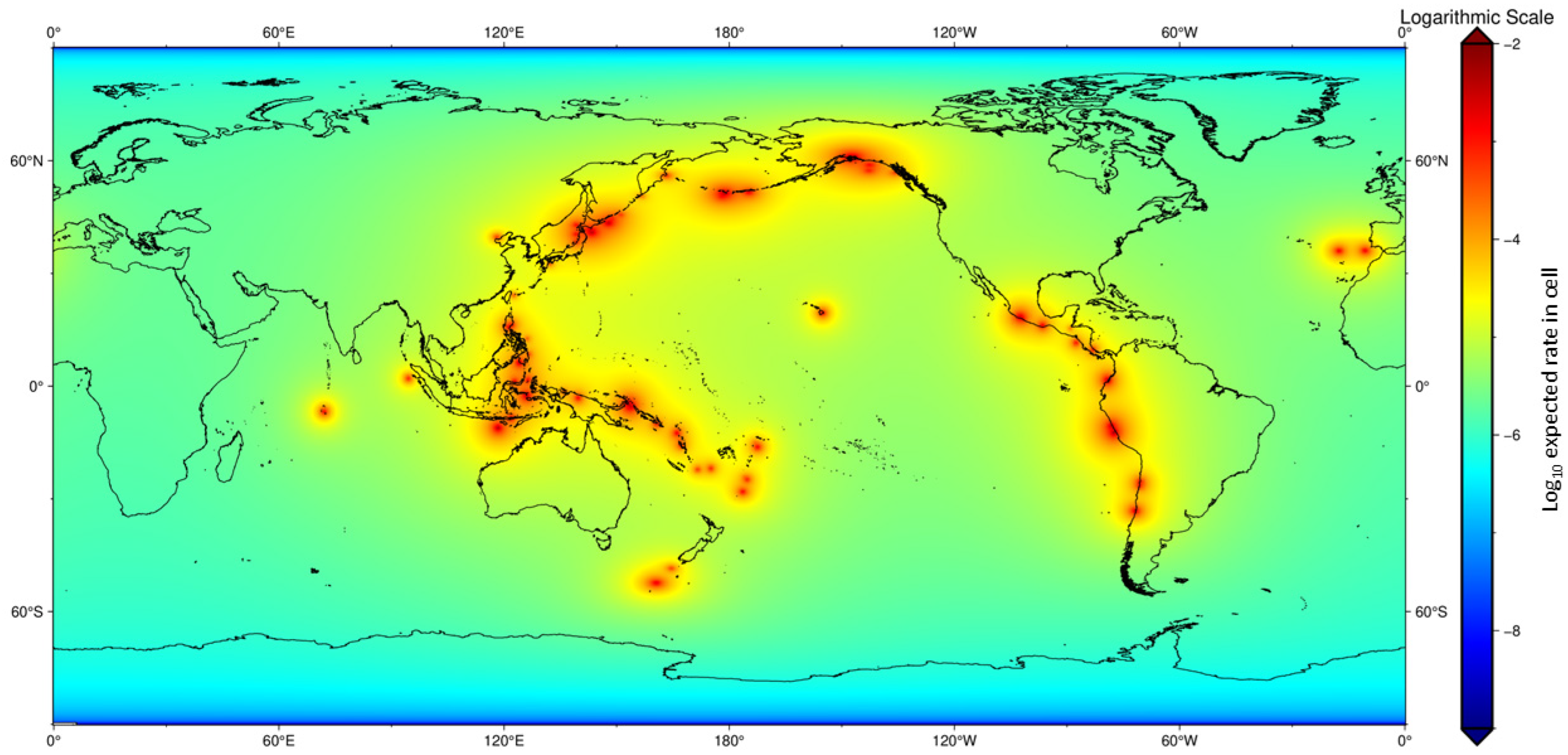
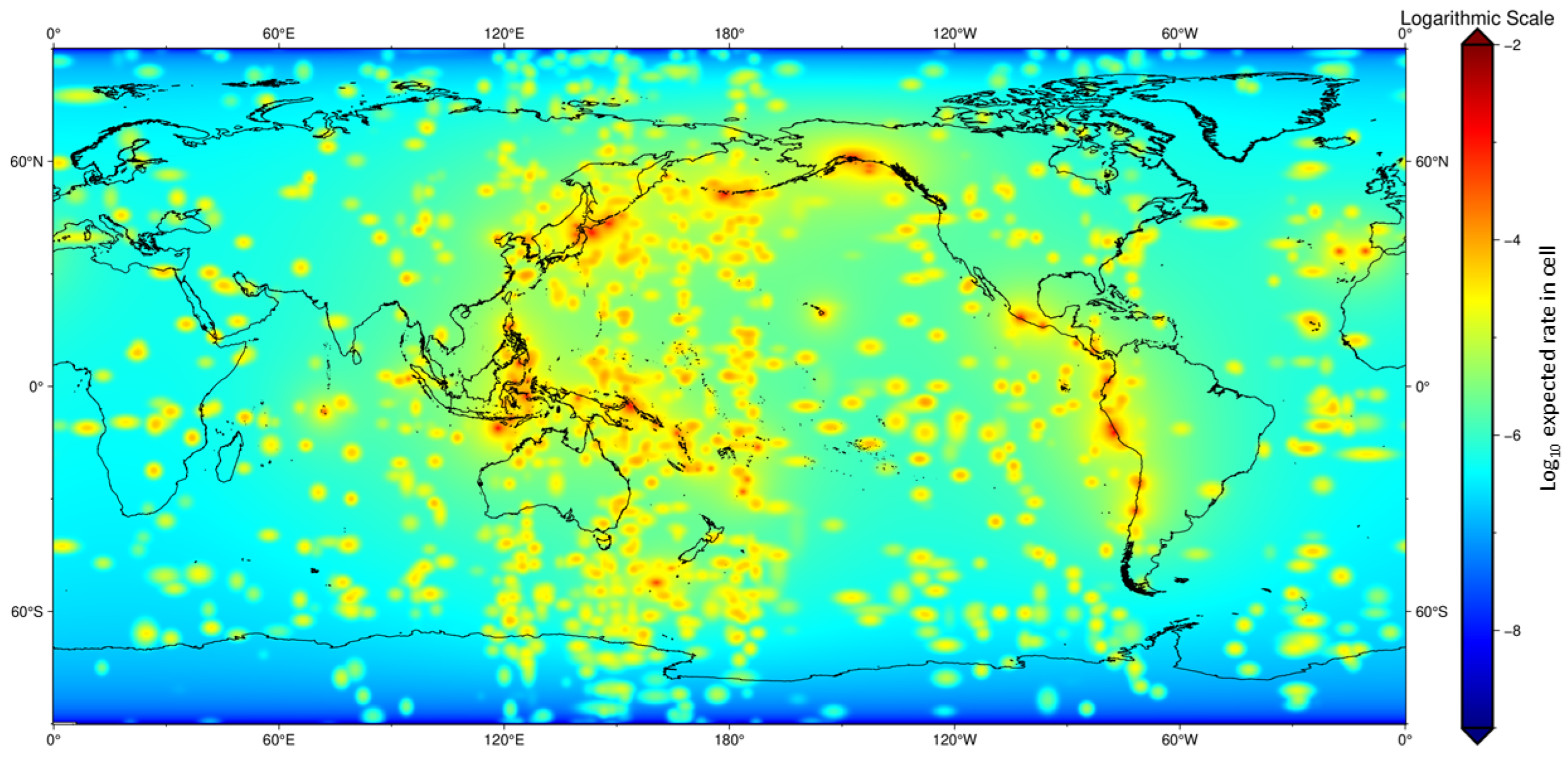
First, the three parameters of the PPE model were optimized (resulting in the values in Table 1). Then, with these parameters fixed, five parameters of the PPE-EEPAS model—$a_M$, $a_T$, ${\mathsf{\sigma }}_A$ and $b_A$ of EEPTV₁ (Table 2) and ${\mu }_{\mathrm{P}\mathrm{P}\mathrm{E}}$ of PPE-EEPAS (Table 3)—were simultaneously optimized, with the other parameters of EEPTV₁—$b_M$, ${\mathsf{\sigma }}_M$, $b_T$ and ${\mathsf{\sigma }}_T$—set at values derived from previous studies (see Table 2). The fixed value of 1.0 for $b_M$ serves to make the difference between a precursor magnitude and the associated target earthquake magnitude distribution independent of magnitude. The other fixed parameters are taken from statistics of the fitted Ψ scaling relations [23], which were derived from multiple regional catalogues. The value of $b_T$ is from the regression parameter of the same name in (1) and the values ${\mathsf{\sigma }}_M$ and ${\mathsf{\sigma }}_T$ are from the residual standard deviations of the regressions of M_m and logT_P, respectively, on M_P. The purpose of this limited optimization was to avoid overfitting of parameters to only 85 target earthquakes. The models GSR-PPE, GSR-EEPAS and GSR-PPE-EEPAS₁ were formed by optimizing the relevant mixing parameters from among ${\mu }_{\mathrm{G}\mathrm{S}\mathrm{R}}$, ${\mu }_{\mathrm{P}\mathrm{P}\mathrm{E}}$ and ${\mu }_{\mathrm{E}\mathrm{E}\mathrm{P}\mathrm{T}\mathrm{V}}$ (Table 3) with all other parameters fixed. Finally, the GSR-PPE-EEPAS₂ model was formed by simultaneously refitting the EEPTV parameters $a_T$ and ${\mathsf{\sigma }}_A$ (EEPTV₂ in Table 2) and the mixing parameters ${\mu }_{\mathrm{G}\mathrm{S}\mathrm{R}}$ and ${\mu }_{\mathrm{P}\mathrm{P}\mathrm{E}}$ (Table 3). The spatial distribution of a 20-year PPE model forecast is displayed in Figure 3, and that of a 20-year PPE-EEPAS model forecast in Figure 4. These figures illustrate how the models have high rate densities close to the locations of their respective inputs—the previous events with M ≥ 7.45 in the case of PPE and those with M ≥ 5.95 in the case of PPE-EEPAS. In both cases, the rate density at locations remote from the input events is controlled by the power law decay of the PPE model spatial kernel (Equation (10)).

Table 2. Parameters of the EEPTV1 and EEPTV2 models as fitted to the period 1994–2013.

Parameter	EEPTV1	EEPTV2	Fitting Range
$a_M$	1.45	1.45 *	1.0–1.5
$b_M$	1.00 *	1.00 *
${\mathsf{\sigma }}_M$	0.32 *	0.32 *
$a_T$	1.20	1.36	1.0–2.0
$b_T$	0.40 *	0.40 *
${\mathsf{\sigma }}_T$	0.23 *	0.23 *
${\mathsf{\sigma }}_A$	4.45	2.95	0.1–10
$b_A$	0.43	0.43 *	0.2–0.6

* Fixed parameter.

Table 3. Models, mixing parameters (see Equation (8)) and information gains per earthquake (IG) over SUP in the fitting period 1994–2013.

Model Name	Model Components	${\mathit{\mu }}_{\mathbf{G}\mathbf{S}\mathbf{R}}$	${\mathit{\mu }}_{\mathbf{P}\mathbf{P}\mathbf{E}}$	${\mathit{\mu }}_{\mathbf{E}\mathbf{E}\mathbf{P}\mathbf{T}\mathbf{V}}$	IG
PPE	PPE		1.0		1.67
PPE-EEPAS	PPE + EEPTV1		0.26	0.74	2.21
GSR	GSR	1.0			1.77
GSR-PPE	GSR + PPE	0.58	0.42		2.12
GSR-EEPAS	GSR + EEPTV1	0.35		0.65	2.37
GSR-PPE-EEPAS1	GSR + PPE + EEPTV1	0.32	0.10	0.58	2.38
GSR-PPE-EEPAS2	GSR + PPE + EEPTV2	0.32	0.14	0.54	2.41

Figure 3. Spatial distribution of the logarithm of the expected number of earthquakes with magnitude $M\ge 7.45$ per cell in a gridded PPE model forecast for the period 1994–2013, based on input data in the period 1964–1993.

Figure 4. Spatial distribution of the logarithm of the expected number of earthquakes with magnitude $M\ge 7.45$ per cell in a gridded PPE-EEPAS model forecast for the period 1994–2013, based on input data in the period 1964–1993.

The information gain [38] per earthquake of one model A over another model B is estimated here by

$$IG\left(A,B\right)={\displaystyle \frac{\ln L_A-\ln L_B}{N}}.$$

(16)

This is the mean information gain over all target earthquakes. From (15) and (16), the information gain for the ith target earthquake is given by

$${IG}_i\left(A,B\right)=\ln {\lambda }_A\left(t_{n_i},m_{n_i},x_{n_i},y_{n_i}\right)-\ln {\lambda }_B\left(t_{n_i},m_{n_i},x_{n_i},y_{n_i}\right)-{\displaystyle \frac{{\widehat{N}}_A-{\widehat{N}}_B}{N}}.$$

(17)

The definition in (16) is strictly appropriate for an independent testing period in which all parameters are fixed. For the fitting period, no adjustment is made here for differences in the number of fitted parameters between models, because the number of fitted parameters to be counted is ambiguous in some cases; the models have up to 18 adjustable parameters, but no more than five are simultaneously optimized in any fitting run. Neglecting the number of fitted parameters means that the IGs in the fitting period are slightly overestimated. In any case, the IGs in an independent testing period are more reliable indicators of model performance than those in the fitting period.

Table 3 shows the fitted component weights (mixing parameters) and information gain per earthquake, IG, of each of the other models over SUP. SUP is used as the reference here because it contains no temporal or spatial information on earthquake occurrence. The other models all contain spatial and, in most cases, temporal information, so they tend to have positive IGs relative to SUP. PPE and GSR contain the same magnitude information as SUP. PPE and GSR contain very different spatial information (see Figure 2 and Figure 3). GSR contains no temporal information. PPE contains only weak temporal information, which changes as target earthquakes are added to the catalogue. EEPTV contains strongly varying temporal information as well as different spatial and magnitude information than all other models. The high values of the mixing parameter ${\mu }_{\mathrm{E}\mathrm{E}\mathrm{P}\mathrm{T}\mathrm{V}}$ (>0.5) in all models containing EEPTV show that there is a strong contribution from EEPTV to these hybrid models. This is further supported by the fact that all models containing EEPTV have higher IGs than all models that do not.

Table 3 further shows that GSR has a greater IG than PPE, and GSR-EEPAS has a greater IG than PPE-EEPAS. Also, GSR-PPE, in which ${\mathsf{\mu }}_{\mathrm{G}\mathrm{S}\mathrm{R}}$ and ${\mathsf{\mu }}_{\mathrm{P}\mathrm{P}\mathrm{E}}$ are similar (0.58 and 0.42, respectively), has an appreciably greater IG than either of its components, GSR and PPE, as individual models. However, the GSR-PPE-EEPAS models have much smaller values of ${\mathsf{\mu }}_{\mathrm{P}\mathrm{P}\mathrm{E}}$ (0.1 and 0.14) than of ${\mathsf{\mu }}_{\mathrm{G}\mathrm{S}\mathrm{R}}$ (0.32) and have IGs not much greater than GSR-EEPAS. This indicates that GSR is better than PPE as a single background model for EEPTV. It is not surprising that GSR-PPE-EEPAS₂ has the highest IG of all, given that EEPTV₂ was optimized for a GSR-PPE background.

3.2. Testing

The performance of the models was next assessed in forecasting target earthquakes in an independent period. The models were tested, with all parameters fixed, over the period 2014–2019, which included 19 target earthquakes with $M\ge 7.45$. For this purpose, the log-likelihood, expected number of target earthquakes and information gain per earthquake relative to SUP were evaluated for each model.

The expected number of earthquakes $\widehat{N}$ and IG of each model are given in Table 4. All models expected more target earthquakes than occurred in the test period, reflecting the higher rate of target earthquakes in the fitting period than in the testing period. However, the expected numbers for all models except PPE do not differ significantly from the observed number at the 0.05 level of significance, according to the standard CSEP N-test [31]. The CSEP N-test assumes a Poisson distribution for the number of earthquakes [31]. It is known that earthquakes are usually more clustered than a Poisson distribution; a negative binomial distribution with higher variance than the Poisson distribution [39] is widely accepted as a more realistic distribution for earthquake numbers. The expected number (31.5) of the PPE model is consistent with the observed number (19) if a negative binomial distribution with any variance greater than 1.35 times that of the Poisson distribution is assumed.

Table 4. Expected number of target earthquakes ($\widehat{N}$) and information gain per earthquake (IG) over SUP of models in the testing period 2014–2019.

Model Name	$$\widehat{\mathit{N}}$$	IG
SUP	25.5	0.00
PPE	31.5 *	1.22
PPE-EEPAS	25.7	2.03
GSR	25.4	1.77
GSR-PPE	28.6	1.86
GSR-EEPAS	24.7	2.27
GSR-PPE-EEPAS1	25.4	2.23
GSR-PPE-EEPAS2	24.8	2.29

* $\widehat{N}$ differs significantly from the observed N (p < 0.05) in the Poisson test.

Comparing the IGs in Table 3 and Table 4, the PPE model has a markedly lower IG in the testing period than in the fitting period. Also, all models that have PPE as a component have lower IGs in the testing period than in the fitting period. In the testing period, the GSR-PPE-EEPAS₁ model has a lower IG than GSR-EEPAS, but GSR-PPE-EEPAS₂ still has the highest IG of all.

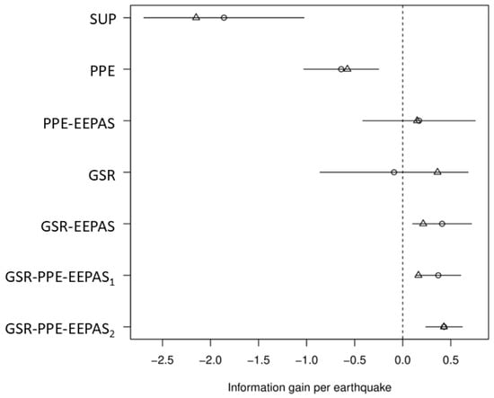
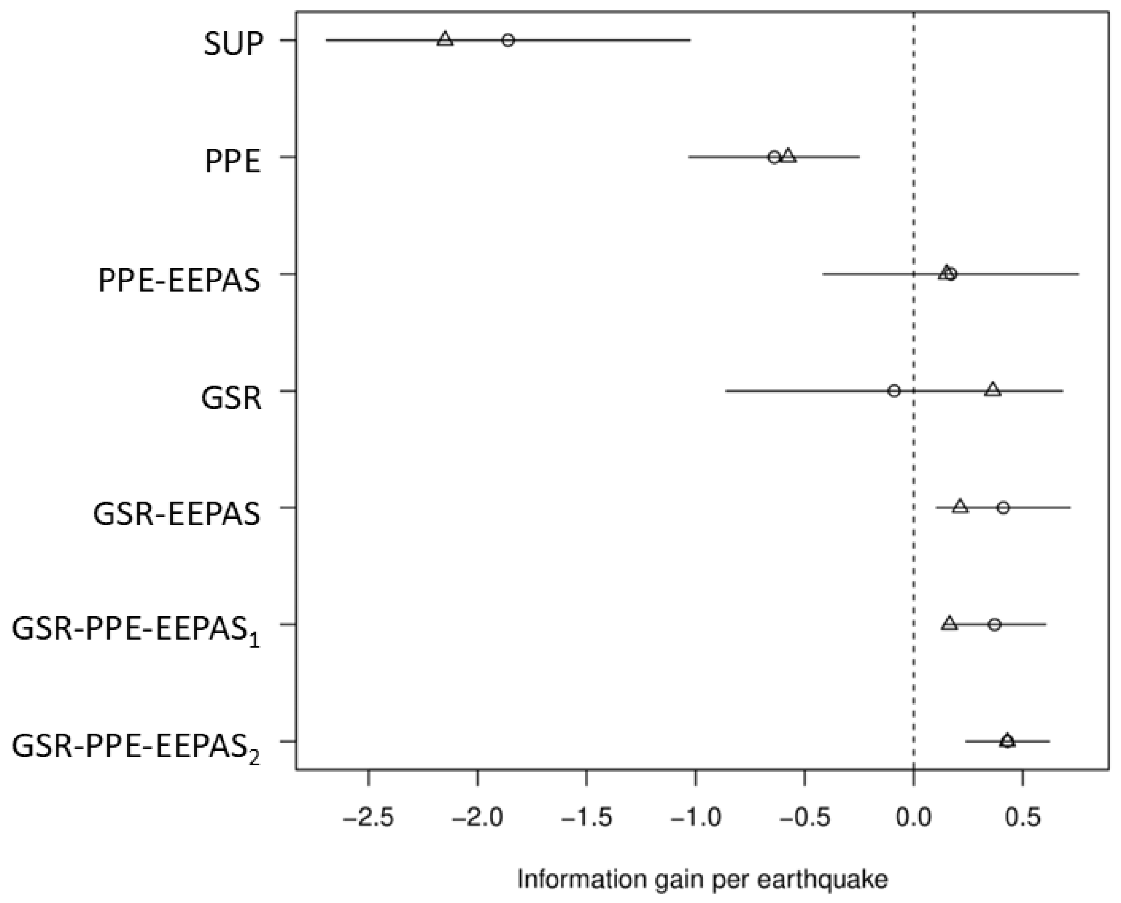
The CSEP t-test [33], a specialized application of the paired Student t-test, is designed to estimate the uncertainty of the mean information gain per earthquake and to assess the statistical significance of the information gain of one model over another. The t-test is applied in Figure 5 to examine the statistical significance of the performance of other models relative to the best background model combination of GSR-PPE in the testing period. It is seen that the models GSR-EEPAS, GSR-PPE-EEPAS₁ and GSR-PPE-EEPAS₂ significantly outperform GSR-PPE in the testing period, and in turn, GSR-PPE outperforms the PPE and SUP models. Figure 5 shows both the mean and median of the information gain per earthquake over the 19 target earthquakes. For all model comparisons, the median lies within the confidence interval for the mean, indicating that the IGs are not overly influenced by a small number of target earthquakes. However, the robustness assessment remains preliminary. Longer testing periods or prospective CSEP-style testing are needed to further verify the stability of the model ranking.

Figure 5. Mean (circles) and median (triangles) of the information gain per earthquake of other models relative to GSR-PPE in the testing period 2014–2019, with 19 target earthquakes. Error bars represent 95% confidence limits of the mean, using the t-test [33]. If an error bar does not intersect the zero vertical dashed line, there is a statistically significant difference in the performance of the model relative to GSR-PPE at the 0.05 level, according to the t-test.

4. Discussion

4.1. Comparison with Regional EEPAS Modelling

This study is important because it is the first time EEPAS has been applied to forecast the highest magnitudes in a global catalogue. Previous applications to regional catalogues have had much lower target magnitude thresholds, with about 90% of the target earthquakes being less than one magnitude unit above the threshold, according to the Gutenberg–Richter relation.

The performance of EEPAS in forecasting global earthquakes above magnitude 7.45 in this study can be compared to that in regional studies with lower target magnitude thresholds [12,14,15,17,18]. The results here indicate that EEPAS may be as effective in global as in regional forecasting. Indeed, the IGs of PPE-EEPAS over PPE in fitting and testing, at 0.54 (Table 3) and 0.81 (Table 4), respectively, are at the high end of values found in regional applications. This is consistent with a study of EEPAS in Japan [14], which found that IG of PPE-EEPAS over PPE increases with increasing m_c. On the other hand, the IGs of GSR-PPE-EEPAS over GSR-PPE here, ranging from 0.26–0.29 in fitting (Table 3) and from 0.37–0.43 in testing (Table 4), are typical of the IGs of PPE-EEPAS over PPE in regional studies.

4.2. Insights from Power Spectral Densities

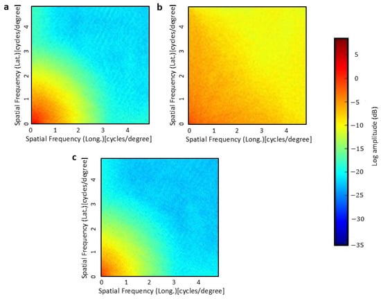
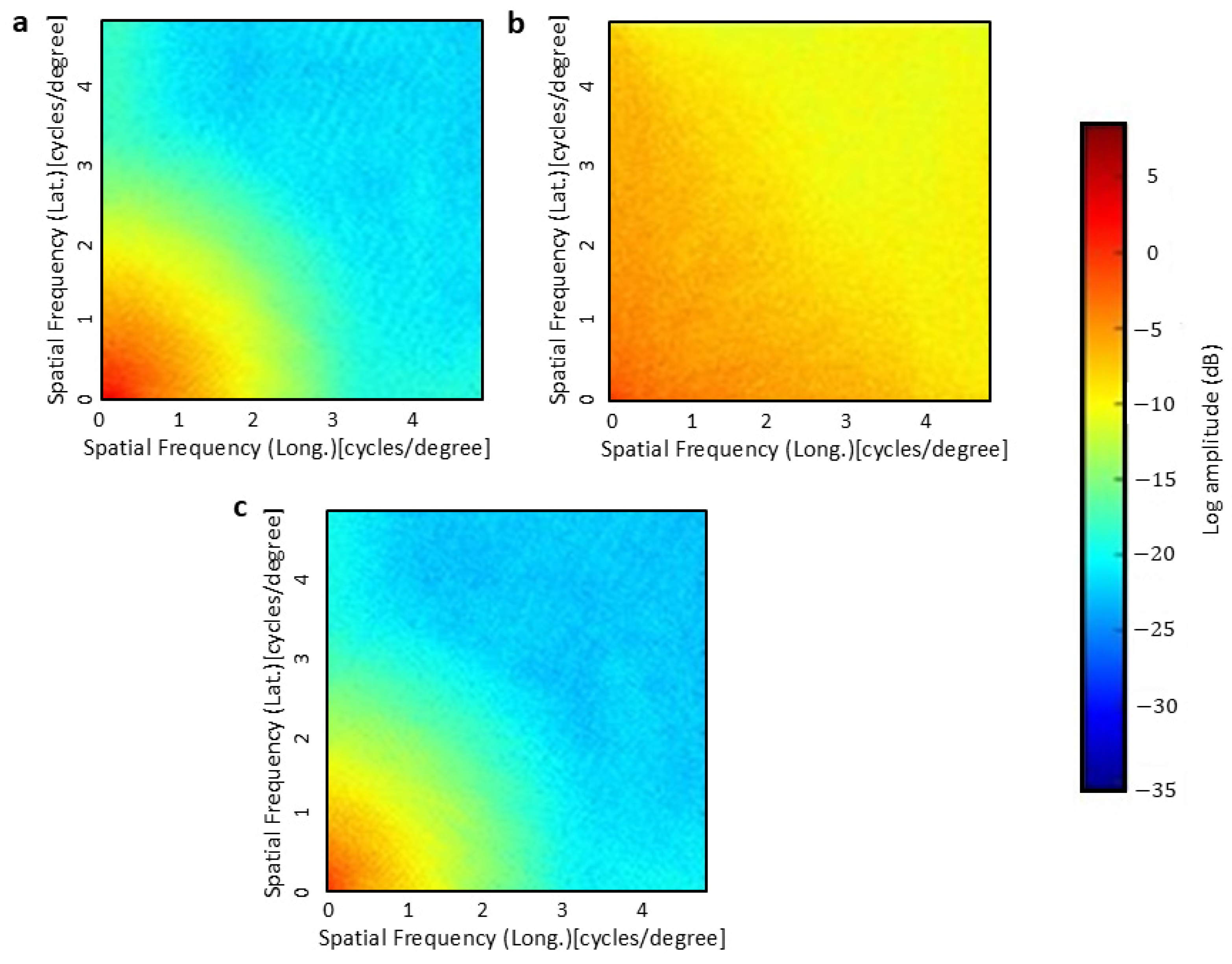
The two-dimensional spatial power spectral density (2-D PSD), the spatial counterpart of the familiar time-series spectrum [40,41,42], can give insights into, but not fully explain, the connection between mixing parameters in hybrid models (Table 3) and spatial resolution. The 2-D PSD (see Appendix A) shows how the variance of a gridded field is distributed over spatial frequencies, which measure how often a pattern is repeated per unit of distance. Low spatial frequencies are associated with long wavelengths that can capture broad, slowly varying structure; high spatial frequencies are associated with short wavelengths that can capture fine texture/noise. Figure 6 displays 2-D PSDs of the spatial distributions of PPE, GSR and PPE-EEPAS models of Figure 2, Figure 3 and Figure 4. It shows that the PPE-EEPAS model concentrates most of its power at low spatial frequencies (<1 cycle/degree), PPE also has power at intermediate frequencies (1–2 cycles/degree), while GSR maintains strong power at higher frequencies (≈3–4 cycles/degree), capturing finer spatial variability close to the grid-resolution limit. Apparently, the relatively smooth low-frequency spatial variation of the PPE-EEPAS model, combined with its strong temporal variation, allows it to match the patterns of earthquake occurrence in the catalogue better than either PPE or GSR. However, the strong power of GSR at high spatial frequencies, where PPE-EEPAS is weak, allows it to make an important contribution to the GSR-PPE-EEPAS hybrids, with the result that these are the best performing models of all.

Figure 6. 2-D power spectral density of (a) PPE, (b) GSR and (c) PPE-EEPAS model as fitted to the ISC-GEM global earthquake catalogue for earthquakes of magnitude $M\ge 7.45$ over the period 1994–2013. The color bar is ${\mathrm{l}\mathrm{o}\mathrm{g}}_{10}\left(\mathrm{P}\mathrm{S}\mathrm{D}\right)$ in dB; warmer colors represent higher power.

4.3. Effects of Global Catalogue Limitations

The limited completeness and duration of global earthquake catalogues present a challenge to global forecasting using the EEPAS model. These limitations affect the choice of magnitude thresholds, the length of the available warm-up period, the number of target earthquakes in the fitting and testing periods and the expected completeness of precursory earthquake contributions to the EEPTV model. They also affect the fitting and performance of models, but in an unknown way.

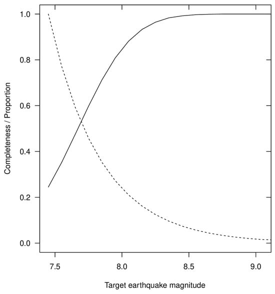
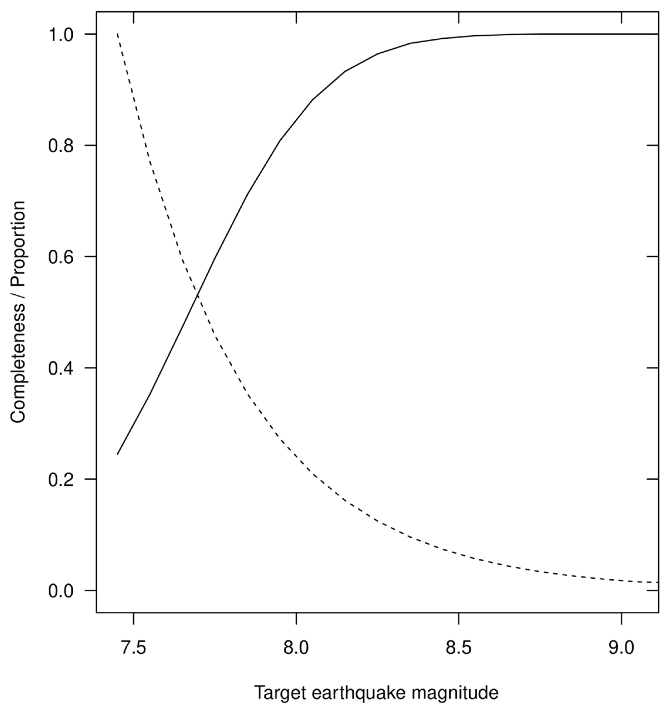
The varying completeness of the catalogue over time affects the choice of magnitude thresholds $m_0$ and $m_c$. The small difference here of 1.5 magnitude units between $m_c$ and $m_c$ is necessitated by these limitations. This is less than in previous EEPAS applications and leads to low completeness $\mathsf{\Delta }\left(m\right)$ of precursory earthquake contributions at the lower end of the target magnitude range (Equation (7)). Figure 7 shows $\mathsf{\Delta }\left(m\right)$ as a function of target earthquake magnitude for the fitted parameters of EEPTV₁ and EEPTV₂, and the proportion of target earthquakes expected to exceed a given magnitude m. It is seen that $\mathsf{\Delta }\left(m\right)$ < ~0.5 for target magnitudes < 7.75, i.e., for about half of all expected target earthquakes. The EEPTV model includes compensation for missing precursors below the input magnitude threshold (Equation (6)), so that it does not underestimate the expected number of target earthquakes. However, the fitted parameters and performance would undoubtedly be different if the catalogue were complete enough to permit a lower value of $m_0$.

Figure 7. Completeness of precursory earthquake contributions above the input magnitude threshold $m_0=5.95$ as a function of target earthquake magnitude, in the EEPTV₁ and EEPTV₂ models (solid line) according to the function Δ(m) of Equation (7), and the proportion of target earthquakes expected to exceed a given magnitude (dashed line) according to the Gutenberg–Richter relation.

It is not possible to specify a minimum satisfactory difference between $m_c$ and $m_0$, because $\mathsf{\Delta }\left(m\right)$ also depends on the parameters $a_M$, $b_M$ and ${\mathsf{\sigma }}_M$ of the magnitude distribution and the Gutenberg–Richter parameter b_EEP (Equation (7), Table 1 and Table 2). A difference of about two magnitude units is usually aimed for. That would mean increasing m_c to about 7.95 in this case. The precursory earthquake set would then be nearly complete for all target earthquakes (Figure 7), but the number of target earthquakes for fitting and testing the models would be drastically reduced to unacceptable levels. Given these considerations, no alternative values of $m_0$ and m_c were entertained. The present threshold combination represents a compromise between catalogue completeness and sample size.

The choice of the warm-up, fitting and testing periods represents a further compromise. Reserving an adequate warm-up period and enough target earthquakes for fitting the models limits the number of target events in the testing set. A longer period of testing, with more target events, would give a more robust result. However, the results obtained here can be corroborated in time by testing against future extensions of the catalogue.

The limited length of the warm-up period, which is 30 years in this study, also affects the completeness of precursory earthquake contributions in the EEPAS model. It is expected that some precursory earthquakes to target events would have occurred before the beginning of the warm-up period. The lead time $t-t_0$ from the beginning of the catalogue to the time of a target earthquake from 30 years to 50 years in the fitting set varies and from 50 years to 55 years in the testing set. The completeness of precursory earthquake contributions within in the time period covered by the catalogue depends on both the time distribution parameters—$a_T$, $b_T$ and ${\mathsf{\sigma }}_T$—and the magnitude distribution parameters—$a_M$, $b_M$ and ${\mathsf{\sigma }}_M$—of EEPTV (Table 2). The proportional completeness $p\left(L,m\right)$ of precursory earthquake contributions as a function of lead time L and target earthquake magnitude m was shown in [43] to be

$$p\left(L,m\right)={\displaystyle \frac{c\left(L,m\right)}{c\left(\infty ,m\right)}},$$

(18)

where

$$c\left(L,m\right)={\int }_{m_0}^{m_u}\left[\mathsf{\Phi }\left({\displaystyle \frac{\log \left(L\right)-a_T-b_T\nu }{{\mathsf{\sigma }}_T}}\right)\right]\eta \left(\nu \right)g\left(m|\nu \right){10}^{-b_{EEP}\nu }d\nu ,$$

(19)

where $\mathsf{\Phi }$ is the standard normal cumulative distribution function, the logarithm is to base 10, and b_EEP is the Gutenberg–Richter b-value (Table 1). The magnitude density $g$ was defined in (3) and the normalizing function $\eta$ in (9).

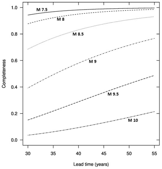
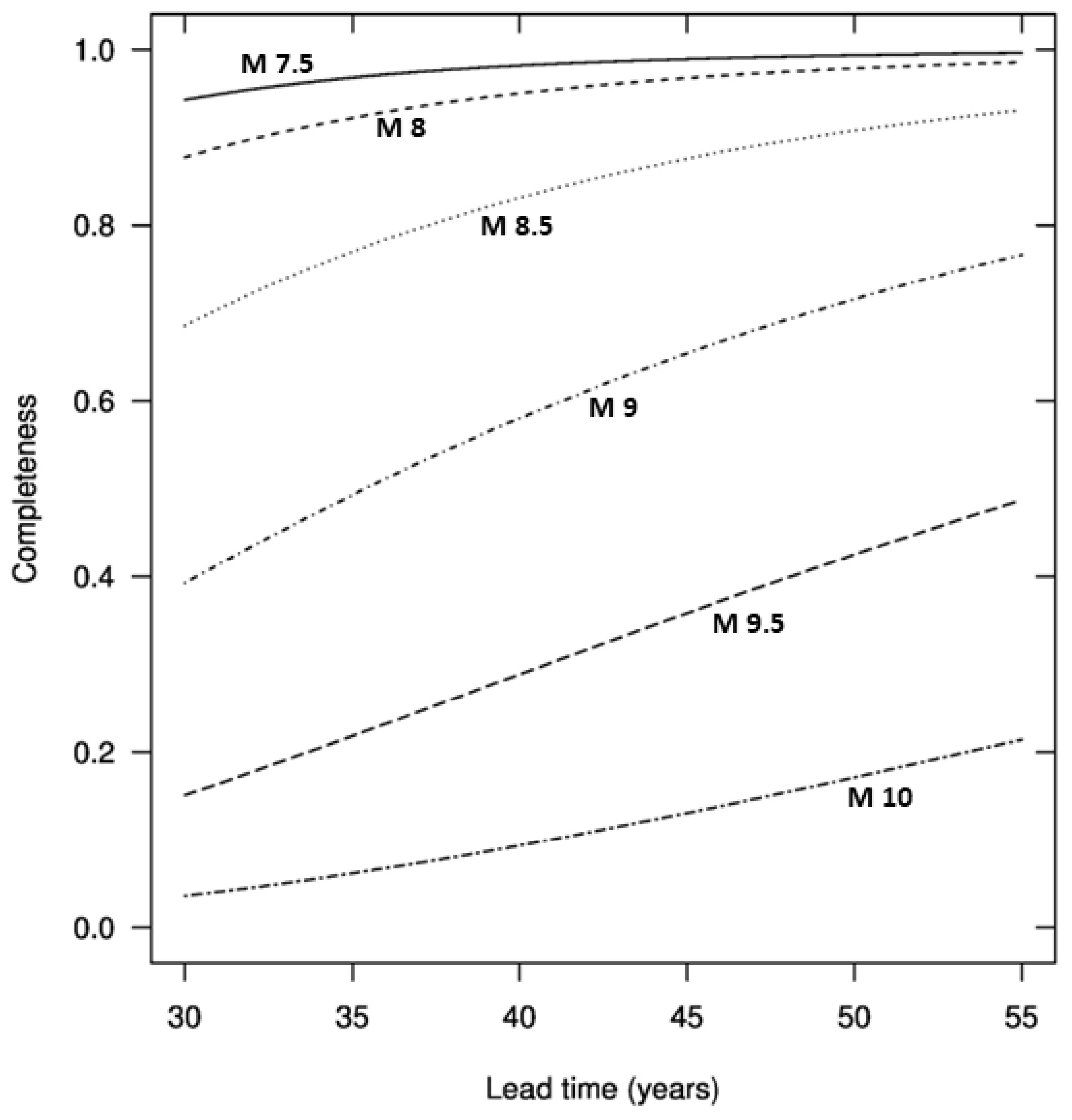
Figure 8 shows the completeness as a function of the lead time for target earthquake magnitudes ranging from 7.5 to 10.0, for the fitted parameters of EEPTV₁ (Table 3). At the beginning of the fitting period, the lead time is 30 years. The precursory earthquakes are then more than 65% complete for target earthquake magnitudes ≤ 8.5, but less than 50% complete for target earthquake magnitudes ≥ 9.0. At the beginning of the testing period, the lead time is 50 years. By that time, the completeness at higher magnitudes has markedly improved, being greater than 70% for magnitudes ≥ 9.0 and greater than 40% for magnitudes ≥ 9.5. No compensation is made here for incompleteness due to the limited lead time. Technical development of the EEPAS model is required to implement compensation for variable lead times for target earthquakes during the fitting and testing periods.

Figure 8. Completeness of precursory earthquake contributions as a function of lead time for target earthquakes with selected magnitudes from M 7.5 to M 10.0 in the fitted EEPTV₁ model.

4.4. Space-Time Trade-Off of Precursory Seismicity

The fitted value of $a_T$ is larger, and the value of ${\mathsf{\sigma }}_A$ smaller, in EEPTV₂ than in EEPTV₁ when the models are optimized with different background components (Table 2). This illustrates a well-known feature of Ψ and EEPAS—the space-time trade-off of precursory seismicity [24]. For many major earthquakes in real and synthetic earthquake catalogues, it is possible to make multiple different identifications with radically different values of A_P and T_P. Statistical analysis of many such multiple identifications has shown that high values of A_P are associated with low values of T_P, and vice versa. There is an approximately even trade-off between time and area [25]. In the EEPAS model, precursor times are proportional to ${10}^{a_T}$ (Equation (2)) and precursory areas to σ_A² (Equation (4)). The space-time trade-off can be exploited to improve forecasting by mixing EEPAS models with ($a_T$,${\mathsf{\sigma }}_A$) pairs chosen from points along the even-trade-off line [44]. This technique has been applied in the 2022 revision of the New Zealand National Seismic Model, which is intended to apply to the next 100 years, with the EEPAS model used to estimate the spatial distribution of earthquake occurrence for the first 20 years [45,46]. Such mixing is not attempted here; how to exploit the space-time trade-off in an optimal way is a problem for future research.

4.5. Seismicity-Rate Dependence of Time Distribution

Another known feature of Ψ and the EEPAS model is that T_P in the Ψ scaling relation for time (Equation (1)) and the parameter $a_T$ in the EEPTV time distribution (Equation (2)) depend on the long-term seismicity rate. Christophersen et al. [24] found in a study of EEPAS fitted to physics-based synthetic catalogues that when the slip rates on all faults in the earthquake simulator were systematically varied by a factor ρ, the variation in 10^aT was inversely proportional to ρ. In the present study, this means that the precursor times for large earthquakes in continental regions are expected to be much longer than those in plate-boundary regions. The restricted length of the global catalogue limits the ability of EEPAS to forecast rare large earthquakes in inactive continental regions.

The strain rate model is treated here as a time-invariant background model, although it is not necessarily time-invariant in the long run. A study in the New Zealand region has shown that strain rates explain the locations of recent large earthquakes ($M\ge 4.95$) better than those of 40–70 years ago [47]. If the same pattern holds for global earthquakes, updating the GSR model will be necessary to maintain its forecasting capability for future earthquakes.

4.6. Reproducibility and Prospective Testing

The results presented here can be reproduced using the EEPAS software package, version eepas_dev43g (see Data availability statement). To independently reproduce the results requires considerable effort involving efficient programming, but not necessarily high-performance computing. The main steps are: (A) computation of the log likelihood (15) of each model for a given parameter set; and (B) finding the maximum-likelihood estimates of the parameters of each model. The calculation of the expected number of earthquakes is the most challenging part of step A, especially the spatial integration over a polygonal testing region, which usually requires numerical approximation. Step B can be accomplished using standard available numerical optimization software.

For a global model, integration of the EEPAS spatial contributions is straightforward because the variances of the bivariate normal densities are small enough that they all integrate to 1 over the whole earth’s surface. The PPE spatial kernels $1/(d^2+r_i^2)$ (Equation (10)) are not integrable over an infinite planar surface; their integrals over the Earth’s surface are of the form

$$I={\int }_0^{\pi }{\displaystyle \frac{2\pi r^2\sin \alpha }{d^2+{\alpha }^2{r}^2}}d\alpha ,$$

(20)

where r is the radius of the Earth. This integral can be approximated using the trapezoidal rule. For a gridded likelihood model like GSR, the expected number of earthquakes is obtained by simply summing over the cell expectations.

Future work will aim to confirm the forecasting performance of our models by submitting them to a rigorous and transparent prospective CSEP-style forecasting experiment, in which the testing is independent of the software that generated the models. This will address several limitations of the present study, including its retrospective nature, the limited data available for testing, and the difficulty of verifying every aspect of the software used or of independently reproducing the results.

5. Conclusions

An initial investigation of EEPAS modelling using a global catalogue suggests that a global EEPAS model can be effective in world-wide forecasting of very large earthquakes with similar information gains over time-invariant or slowly evolving background models as in regional applications. The target magnitude threshold for global forecasting cannot be lowered much below 7.5, given the present length and limited completeness of global catalogues. Future improvements to EEPAS modelling, especially optimization of the space-time trade-off, allowance for earthquake rate dependence of the mean of the EEPAS time distribution and compensation for the variable lead-times of target earthquakes, are expected to improve both regional and global forecasting using the EEPAS model. This study has demonstrated that using a strain rate background model as well as, or instead of, a smoothed seismicity background model improves EEPAS forecasts. Attempting further improvements to background modeling is another way of improving EEPAS model performance. Future transparent CSEP-style testing will consolidate understanding of the forecasting performance of the global models presented here.

References

- Jordan, T.H. Earthquake Predictability, Brick by Brick. Seismol. Res. Lett. 2006, 77, 3–6. [Google Scholar] [CrossRef] [Scilit]
- Zechar, J.D.; Schorlemmer, D.; Liukis, M.; Yu, J.; Euchner, F.; Maechling, P.J.; Jordan, T.H. The Collaboratory for the Study of Earthquake Predictability perspective on computational earthquake science. Concurr. Comput. Pract. Exp. 2010, 22, 1836–1847. [Google Scholar] [CrossRef] [Scilit]
- Iturrieta, P.; Savran, W.H.; Herrmann, M.; Bayona, J.A.; Gerstenberger, M.C.; Graham, K.; Maechling, P.J.; Marzocchi, W.; Mizrahi, L.; Schorlemmer, D.; et al. floatCSEP: An application to deploy and conduct reproducible prospective earthquake forecasting experiments. Open J. 2026, 11, 9408. [Google Scholar] [CrossRef] [Scilit]
- Mizrahi, L.; Dallo, I.; van der Elst, N.J.; Christophersen, A.; Spassiani, I.; Werner, M.J.; Iturrieta, P.; Bayona, J.A.; Iervolino, I.; Schneider, M.; et al. Developing, Testing, and Communicating Earthquake Forecasts: Current Practices and Future Directions. Rev. Geophys. 2024, 62, e2023RG000823. [Google Scholar] [CrossRef] [Scilit]
- Ogata, Y. Space-Time Point-Process Models for Earthquake Occurrences. Ann. Inst. Stat. Math. 1998, 50, 379–402. [Google Scholar] [CrossRef] [Scilit]
- Gerstenberger, M.C.; Jones, L.M.; Wiemer, S. Short-term aftershock probabilities: Case studies in California. Seismol. Res. Lett. 2007, 78, 66–77. [Google Scholar] [CrossRef] [Scilit]
- Zhuang, J.; Ogata, Y.; Vere-Jones, D.; Ma, L.; Guan, H. Chapter 7. Statistical Modeling of Earthquake Occurrences Based on External Geophysical Observations: With an Illustrative Application to the Ultra-low Frequency Ground Electric Signals Observed in the Beijing Region. In Seismic Imaging, Fault Damage and Heal; Yong-Gang, L., Ed.; De Gruyter: Berlin, Germany; Boston, MA, USA, 2014; pp. 351–378. [Google Scholar]
- Cattania, C.; Hainzl, S.; Wang, L.; Roth, F.; Enescu, B. Propagation of Coulomb stress uncertainties in physics-based aftershock models. J. Geophys. Res. Solid Earth 2014, 119, 7846–7864. [Google Scholar] [CrossRef] [Scilit]
- Baker, J.; Bradley, B.; Stafford, P. Seismic Hazard and Risk Analysis; Cambridge University Press: Cambridge, UK, 2021. [Google Scholar]
- Stirling, M.; McVerry, G.; Gerstenberger, M.; Litchfield, N.; Van Dissen, R.; Berryman, K.; Barnes, P.; Wallace, L.; Villamor, P.; Langridge, R.; et al. National Seismic Hazard Model for New Zealand: 2010 Update. Bull. Seismol. Soc. Am. 2012, 102, 1514–1542. [Google Scholar] [CrossRef] [Scilit]
- Gerstenberger, M.C.; Bora, S.; Bradley, B.A.; DiCaprio, C.; Kaiser, A.; Manea, E.F.; Nicol, A.; Rollins, C.; Stirling, M.W.; Thingbaijam, K.K.S.; et al. The 2022 Aotearoa New Zealand National Seismic Hazard Model: Process, Overview, and Results. Bull. Seismol. Soc. Am. 2023, 114, 7–36. [Google Scholar] [CrossRef] [Scilit]
- Rhoades, D.A.; Evison, F.F. Long-range Earthquake Forecasting with Every Earthquake a Precursor According to Scale. Pure Appl. Geophys. 2004, 161, 47–72. [Google Scholar] [CrossRef] [Scilit]
- Gerstenberger, M.C.; Christophersen, A.; Rhoades, D.A. A Review of 15 Years of Public Earthquake Forecasting in Aotearoa New Zealand. Seismol. Res. Lett. 2024, 95, 3416–3432. [Google Scholar] [CrossRef] [Scilit]
- Rhoades, D.A.; Evison, F.F. Test of the EEPAS Forecasting Model on the Japan Earthquake Catalogue. Pure Appl. Geophys. 2005, 162, 1271–1290. [Google Scholar] [CrossRef] [Scilit]
- Console, R.; Rhoades, D.A.; Murru, M.; Evison, F.F.; Papadimitriou, E.E.; Karakostas, V.G. Comparative performance of time-invariant, long-range and short-range forecasting models on the earthquake catalogue of Greece. J. Geophys. Res. Solid Earth 2006, 111, B09304. [Google Scholar] [CrossRef] [Scilit]
- Biondini, E.; Rhoades, D.A.; Gasperini, P. Application of the EEPAS earthquake forecasting model to Italy. Geophys. J. Int. 2023, 234, 1681–1700. [Google Scholar] [CrossRef] [Scilit]
- Schneider, M.; Clements, R.; Rhoades, D.; Schorlemmer, D. Likelihood- and residual-based evaluation of medium-term earthquake forecast models for California. Geophys. J. Int. 2014, 198, 1307–1318. [Google Scholar] [CrossRef] [Scilit]
- Rhoades, D.A.; Christophersen, A.; Gerstenberger, M.C.; Liukis, M.; Silva, F.; Marzocchi, W.; Werner, M.J.; Jordan, T.H. Highlights from the First Ten Years of the New Zealand Earthquake Forecast Testing Center. Seismol. Res. Lett. 2018, 89, 1229–1237. [Google Scholar] [CrossRef] [Scilit]
- Tsuruoka, H.; Hirata, N.; Schorlemmer, D.; Euchner, F.; Nanjo, K.Z.; Jordan, T.H. CSEP Testing Center and the first results of the earthquake forecast testing experiment in Japan. Earth Planets Space 2012, 64, 661–671. [Google Scholar] [CrossRef] [Scilit]
- Kreemer, C.; Blewitt, G.; Klein, E.C. A geodetic plate motion and Global Strain Rate Model. Geochem. Geophys. Geosystems 2014, 15, 3849–3889. [Google Scholar] [CrossRef] [Scilit]
- Bird, P.; Jackson, D.D.; Kagan, Y.Y.; Kreemer, C.; Stein, R.S. GEAR1: A Global Earthquake Activity Rate Model Constructed from Geodetic Strain Rates and Smoothed Seismicity. Bull. Seismol. Soc. Am. 2015, 105, 2538–2554. [Google Scholar] [CrossRef] [Scilit]
- Bayona, J.A.; Savran, W.; Strader, A.; Hainzl, S.; Cotton, F.; Schorlemmer, D. Two global ensemble seismicity models obtained from the combination of interseismic strain measurements and earthquake-catalogue information. Geophys. J. Int. 2020, 224, 1945–1955. [Google Scholar] [CrossRef] [Scilit]
- Evison, F.F.; Rhoades, D.A. Demarcation and Scaling of Long-term Seismogenesis. Pure Appl. Geophys. 2004, 161, 21–45. [Google Scholar] [CrossRef] [Scilit]
- Christophersen, A.; Rhoades, D.A.; Colella, H.V. Precursory seismicity in regions of low strain rate: Insights from a physics-based earthquake simulator. Geophys. J. Int. 2017, 209, 1513–1525. [Google Scholar] [CrossRef] [Scilit]
- Christophersen, A.; Rhoades, D.A.; Hainzl, S. Algorithmic Identification of the Precursory Scale Increase Phenomenon in Earthquake Catalogs. Seismol. Res. Lett. 2024, 95, 3464–3481. [Google Scholar] [CrossRef] [Scilit]
- Gutenberg, B.; Richter, C.F. Frequency of Earthquakes in California. Bull. Seismol. Soc. Am. 1944, 34, 185–188. [Google Scholar] [CrossRef] [Scilit]
- Jackson, D.D.; Kagan, Y.Y. Testable Earthquake Forecasts for 1999. Seismol. Res. Lett. 1999, 70, 393–403. [Google Scholar] [CrossRef] [Scilit]
- Di Giacomo, D.; Harris, J.; Villaseñor, A.; Storchak, D.A.; Engdahl, E.R.; Lee, W.H.K. ISC-GEM: Global Instrumental Earthquake Catalogue (1900–2009), I. Data collection from early instrumental seismological bulletins. Phys. Earth Planet. Inter. 2015, 239, 14–24. [Google Scholar] [CrossRef] [Scilit]
- Michael, A.J. How Complete is the ISC-GEM Global Earthquake Catalog? Bull. Seismol. Soc. Am. 2014, 104, 1829–1837. [Google Scholar] [CrossRef] [Scilit]
- Schorlemmer, D.; Gerstenberger, M.C. RELM Testing Center. Seismol. Res. Lett. 2007, 78, 30–36. [Google Scholar] [CrossRef] [Scilit]
- Schorlemmer, D.; Gerstenberger, M.C.; Wiemer, S.; Jackson, D.D.; Rhoades, D.A. Earthquake Likelihood Model Testing. Seismol. Res. Lett. 2007, 78, 17–29. [Google Scholar] [CrossRef] [Scilit]
- Rhoades, D.A.; Christophersen, A.; Gerstenberger, M.C. Multiplicative earthquake likelihood models incorporating strain rates. Geophys. J. Int. 2017, 208, 1764–1774. [Google Scholar] [CrossRef] [Scilit]
- Rhoades, D.A.; Schorlemmer, D.; Gerstenberger, M.C.; Christophersen, A.; Zechar, J.D.; Imoto, M. Efficient testing of earthquake forecasting models. Acta Geophys. 2011, 59, 728–747. [Google Scholar] [CrossRef] [Scilit]
- Aki, K. Maximum likelihood estimate of b in the formula logN=a-bM and its confidence limits. Bull. Earthq. Res. Inst. 1965, 43, 237–239. [Google Scholar]
- Nelder, J.A.; Mead, R. A simplex method for function minimization. Comput. J. 1965, 7, 308–313. [Google Scholar] [CrossRef] [Scilit]
- Ogata, Y. Estimation of the parameters in the modified Omori formula for aftershock frequecies by the maximium likelihood procedure. J. Phys. Earth 1983, 31, 115–124. [Google Scholar] [CrossRef] [Scilit]
- Ogata, Y. Space-time model for regional seismicity and detection of crustal stress changes. J. Geophys. Res.-Solid Earth 2004, 109, B03308. [Google Scholar]
- Vere-Jones, D. Probabilities and Information Gain for Earthquake Forecasting. In Selected Papers from Volume 30 of Vychislitel’naya Seysmologiya; American Geophysical Union: Washington, DC, USA, 2003; Volume 5, pp. 104–114. [Google Scholar]
- Kagan, Y.Y. Statistical distributions of earthquake numbers: Consequence of branching process. Geophys. J. Int. 2010, 180, 1313–1328. [Google Scholar] [CrossRef] [Scilit]
- Bracewell, R.N. The Fourier Transform and Its Applications; McGraw Hill: Noida, India, 2000. [Google Scholar]
- Oppenheim, A.V.; Schafer, R.W. Discrete-Time Signal Processing, 3rd ed.; Prentice Hall: Hoboken, NJ, USA, 1999. [Google Scholar]
- Percival, D.B.; Walden, A.T. Spectral Analysis for Physical Applications; Cambridge University Press: Cambridge, UK, 1993. [Google Scholar]
- Rhoades, D.A.; Rastin, S.J.; Christophersen, A. The Effect of Catalogue Lead Time on Medium-Term Earthquake Forecasting with Application to New Zealand Data. Entropy 2020, 22, 1264. [Google Scholar] [CrossRef] [Scilit] [PubMed]
- Rastin, S.J.; Rhoades, D.A.; Christophersen, A. Space–Time Trade-Off of Precursory Seismicity in New Zealand and California Revealed by a Medium-Term Earthquake Forecasting Model. Appl. Sci. 2021, 11, 10215. [Google Scholar]
- Rastin, S.J.; Rhoades, D.A.; Rollins, C.; Gerstenberger, M.C.; Christophersen, A.; Thingbaijam, K.K.S. Spatial Distribution of Earthquake Occurrence for the New Zealand National Seismic Hazard Model 2022. Bull. Seismol. Soc. Am. 2024, 114, 2767–2788. [Google Scholar] [CrossRef] [Scilit]
- Gerstenberger, M.C.; Van Dissen, R.; Rollins, C.; DiCaprio, C.; Thingbaijim, K.K.S.; Bora, S.; Chamberlain, C.; Christophersen, A.; Coffey, G.L.; Ellis, S.M.; et al. The Seismicity Rate Model for the 2022 Aotearoa New Zealand National Seismic Hazard Model. Bull. Seismol. Soc. Am. 2024, 114, 182–216. [Google Scholar] [CrossRef] [Scilit]
- Rastin, S.J.; Rhoades, D.A.; Rollins, C.; Gerstenberger, M.C. How Useful Are Strain Rates for Estimating the Long-Term Spatial Distribution of Earthquakes? Appl. Sci. 2022, 12, 6804. [Google Scholar] [CrossRef] [Scilit]
Disclaimer/Publisher’s Note: The statements, opinions and data contained in all publications are solely those of the individual author(s) and contributor(s) and not of MDPI and/or the editor(s). MDPI and/or the editor(s) disclaim responsibility for any injury to people or property resulting from any ideas, methods, instructions or products referred to in the content. |
© 2026 by the authors. Licensee MDPI, Basel, Switzerland. This article is an open access article distributed under the terms and conditions of the Creative Commons Attribution (CC BY) license.