Evaluating Catchment-Scale Physically Based Modeling of Sediment Deposition During an Extreme Rainfall Event

Emtehani, Sobhan; Jetten, Victor; Westen, Cees van; van den Bout, Bastian

doi:10.3390/geosciences16020088

Abstract

Extreme rainfall events often trigger landslides, debris flows, and sediment-laden floods that cause severe damage in built-up areas, yet sediment deposition is rarely quantified in hazard assessments. This study evaluates the capability of the physically based catchment model LISEMHazard to reconstruct sediment generation, transport, and deposition during Hurricane Maria (2017) in two catchments in Dominica (Coulibistrie and Grand Bay). Simulations were performed at 10 m resolution using rainfall, topography, soil, and land-use data. Model calibration and validation used mapped landslides and debris flows, field measurements of deposition height, and DEMs of Difference (DoDs). LISEMHazard reproduced the general magnitude of sediment volumes and the frequency–area distribution of medium and large landslides but showed poor ability to predict their exact locations and overestimated landslide depth and deposition height. Agreement between modeled and observed debris-flow patterns was good in major channels but weak in minor ones. Sensitivity analysis indicated that soil depth and cohesion dominate uncertainties, whereas saturated hydraulic conductivity and surface roughness exert minimal influence. Despite substantial data and model limitations, physically based modeling remains a practical approach for spatial estimation of sediment deposition needed for risk assessment, structural damage evaluation, and cleanup cost estimation.

Keywords:

sediment deposition; debris flows; physically based modeling; LISEMHazard; landslide–flood interactions; catchment-scale processes; hurricane Maria; sensitivity analysis; uncertainty assessment

1. Introduction

Sediment deposition due to floods and debris flows in built-up environments causes significant damage to infrastructure and public and private properties. The most substantial portion of the costs comes from cleaning operations, removal of blockage in drainage and sewage systems, and from repairing the damage caused by sediments and water to the contents of buildings [1,2,3].

There is a continuum between clear water floods and debris flows, depending on the percentage of sediments, and flood analysis should not only focus on water. Although river floods and flash floods mostly consist of water, they contain certain amounts of sediments as well, which in many cases is ignored in flood hazard assessments [4]. If the overland flow is mixed with surface erosion, these sediments are often fine grained and result in muddy deposits [5,6]. If the overland flow is mixed with debris from landslides, the resulting flash floods have properties of debris flows, with fine grains to large boulders (see Figure 1). High concentrations of sediment alter flow properties, where specific density and viscosity start playing a role in the calculations of velocity and discharge [7]. Generally, this happens when more than 50% of the flow volume consists of sediments. Studies are mainly focused on sediments originating from one specific process (e.g., landslides), while in reality, the deposited sediments can be generated by a mixture of different processes that potentially interact with each other. This study considers sediment as an integral part of (flash) flood hazard analysis.

Figure 1. Debris and sediment deposition around a building in Castle Comfort, Dominica, following extreme rainfall during Hurricane Maria.

The erosion processes have been studied extensively [8,9,10,11,12]. Muddy floods are well known (e.g., [6]) but often considered as offsite or downstream effects (depending on the scope of the investigation). Surprisingly, while it is considered one of the main reasons for erosion and conservation research, damages/costs incurred by sediment deposition are not quantified. Impact damage by debris flows is well established [13,14,15], but often for detailed landslide investigation and not coupled to surface erosion and flashfloods. There are groups of models that simulate runoff and erosion (but not flashfloods) (e.g., Hairsine-Rose model), there are models that simulate flashfloods but rarely take sediments into account (e.g., MARINE), and there are models that simulate mass movement and runout (e.g., FLO-2D). From the commonly used models (Table 1), only LISEM can couple eroded sediment from source areas to a sediment laden flood downstream, simulated with a dynamic wave. The classic version “OpenLISEM” simulates surface erosion by runoff, while the branch ‘LISEMHazard’ has introduced two phase flow that simulates course sediments and viscous flow so that debris flows and mudflows can be simulated. This version is used in this research.

Many models have been developed for simulating debris flow hazard. However, most are focused on the estimation of impact pressure [16,17,18]. However, quantification of damages/costs is not complete without having an estimation of the sediment deposition volume. To determine the sediment deposition, it is essential to investigate the sediment source (erosion and slope failure), sediment transport, and entrainment processes.

As shown by Table 1, LISEMHazard is capable of simulating all desired processes and is, therefore, selected for our simulations. More instances of application of OpenLISEM can be found in the literature compared to LISEMHazard. OpenLISEM is used in many studies for simulation of soil erosion and hydrology (Chen, et al. [19], Baartman, et al. [20], Kværnø and Stolte [21], Rahmati, et al. [22], Clutario and David [23], Ferket, et al. [24], Nurritasari, et al. [25]). LISEMHazard is useful for cases in which slope failures and their runouts are present. For instance, de Vugt [26] investigated the occurrence of landslides and floods in St. Eustatius by modeling these hazards using LISEMHazard. They also performed a sensitivity analysis and concluded that the model is most sensitive to cohesion, internal friction angle, soil depth, and initial soil moisture. Xiao [27] applied LISEMHazard to earthquake-triggered slope failures and debris flows in Wenchuan, China in order to analyze the predictive capacity of physically based models. van den Bout, et al. [28] modeled a multi-hazard chain event in a watershed in Wenchuan, China using LISEMHazard. They simulated the co-seismic landslides which led to a landslide dam and a debris flow which later breached the landslide dam. Simulations are useful for reconstructing the flow patterns and sediment deposition characteristics. However, small variations in the uncertain input parameters might significantly influence the simulation outcomes [29]. Most erosion models are calibrated and validated with sediment concentrations in the stream flow at the outlet of a catchment under investigation. Spatial validation of erosion and deposition patterns is very rare (see e.g., Takken, et al. [30]). She concluded that the model was not very good at reproducing detailed field patterns of deposition, but also that deposition amounts were hard to quantify. This highlights the necessity of uncertainty quantification which can be performed through sensitivity analysis. Sensitivity analysis is also useful for systematic calibration of a model and determination of priorities for field data collection [31,32,33,34,35].

Table 1. Available models for simulation of sediment-related processes.

The objective of this research is to evaluate the reliability of the physically based model LISEMHazard for simulation of the sediment deposition patterns and volumes caused by extreme events. This is useful for prediction of potential damage caused by sediment in such circumstances. A fundamental question is if physically based models have reached sufficient spatial accuracy to be used for added risk assessment from sediments. If the modeling results have significant uncertainties, the magnitude of uncertainties is important to quantify. It is also intended to specify the most sensitive variables of LISEMHazard with regards to the volume of generated, deposited, and outflowed sediments. For this purpose, the mass movement process during Hurricane Maria in Coulibistrie and Grand Bay catchments of Dominica was simulated with LISEMHazard. We performed physically based modeling to reconstruct a sediment deposition event. We calibrated the model using observed data and estimated the volume of generated, deposited, and outflowed sediments (out of the catchment into the sea) from simulation outputs.

2. Materials and Methods

2.1. Study Area

Dominica (15°25′ N, 61°21′ W) is a Caribbean island located about halfway between the French islands of Guadeloupe and Martinique in the Eastern Caribbean Sea. The Commonwealth of Dominica is 46 km in length and 17 km in width, and it has an area of about 750 (km²) [76,77]. The island is predominantly covered by rainforest, and the canopy is fairly complete [78]. The topography is young and rugged, and the geology is volcanic and dynamic with a lot of ignimbrite rocks which are easily eroded, especially in a wet tropical environment [79,80]. The central mountain ridge runs from Cape Melville in the north to the steep southern coastal cliffs of Dominica [81,82,83]. Dominica has numerous mountain rivers and streams which flow outward to the ocean but none of them are navigable [81,82,83,84]. Steep slopes, geology, soil, deforestation, numerous rivers, and human activity are the factors favoring the occurrence of mass movement processes in Dominica [85]. Soils are mostly residual soils which are formed by chemical weathering process due to warm temperatures of the island and abundant rainfall [86,87,88]. The meteorological stations at the Melville Hall and Canefield airports have reported the total annual average rainfall of 2650 mm and 1760 mm respectively [89,90]. The dry season runs from December to May and the wet season from June to November and the average annual temperature is 27.5 °C [89,90].

Most communities are located at the mouth of rivers, which makes them exposed to (flash) floods and debris flows from upstream; others located inland are threatened by landslides and debris flows. Communities are connected through the round-island road network which was completed in 1980s despite the technical difficulties imposed by Dominica’s mountainous terrain and friable volcanic rock [81,82,83].

On 18 September 2017, hurricane Maria made landfall on Dominica. Intense rainfall and uprooting of trees during Maria, triggered close to 10,000 landslides, debris flows, and river floods in Dominica, devastating the island and its people, damaging more than 85 percent of houses, and affecting more than 92 percent of the population [91,92]. The extreme surface runoff and stream discharge during hurricane Maria, rapidly transported massive amount of sediments and debris generated by erosion and landslide processes [92]. Shoreline infrastructure was damaged by the coarse sediment and tree debris which were discharged to the sea and were transported back onto the coastline by the storm surge [93,94]. Also, sediments and debris carried by floods filled up the channels and jammed under bridges, intensifying the flooding situation upstream, causing countless roadblocks in different parts of the island and damage to facilities and infrastructure [95,96].

This study was focused on two catchments in Dominica which were heavily affected by sediment deposition: Coulibistrie and Grand Bay. Coulibistrie is located on the coast on the west side of the island and it experienced severe flooding and debris flow during the event. Grand Bay, located in the southern part of the island, was impacted by landslides and debris flows. Figure 2 shows the location of these catchments.

Figure 2. Location of study areas (Coulibistrie and Grand Bay catchments) shown on elevation map of Dominica. Landslides and runouts are indicated in red. The two catchments are shown by hatched polygons. The landslides and debris runouts are derived from satellite image interpretation (see Charim.net).

2.2. Application of LISEMHazard in Dominica

2.2.1. Model Description

LISEMHazard is physically- and raster-based and it is developed for simulating erosion, flooding, slope failure, and mass movement processes on a catchment scale [74]. LISEMHazard incorporates both hydrological processes (e.g., rainfall, interception, infiltration) and morphological processes (e.g., shallow landslides, slope failure, landslide runout) [74]. All flow on the surface and in channels is done with a dynamic wave (shallow Saint-Venant equations). Figure 3 is a flowchart showing the processes of this model. The governing equations of LISEMHazard are described in detail by Bout, et al. [74] and Bout and Jetten [97]. A summary of these equations and description of their variables is given in Table A1 and Table A2 in the Appendix A. All simulations were performed with LISEMHazard version 1.11 and cell size of 10 m and timestep of 10 s. Note that the dynamic wave uses a semi-explicit volume solution with a varying timestep to achieve numerical stability (see e.g., Delestre, et al. [98]).

Figure 3. Flow chart indicating the processes of the LISEMHazard model adapted from Bout, et al. [74]. “ET” stands for evapotranspiration. Red elements indicate soil and sediment dynamics, while blue elements indicate water balance and hydrological processes.

2.2.2. Model Input Data

LISEMHazard is set up in such a way that many parameters in the equations in Table A1 (in Appendix A) are input data, to give the user maximum control. Input variables can be derived from six main datasets: (i) precipitation, (ii) DEM, (iii) channels, (iv) land use/cover, (v) soils, and (vi) buildings and roads. Data sources are briefly described in Table 2. All input data is provided in the form of raster maps.

Precipitation

Rainfall data was obtained from the ground-station in Canefield airport of Dominica located approximately two kilometers north of Roseau. This station was the only one out of six available stations that provided a full record of the hurricane Maria in Dominica, as the other stations malfunctioned during the hurricane. This causes a high level of uncertainty in the input rainfall data. The rainfall data was available with 10-min timesteps. We assumed that a spatial similarity of the precipitation exists for the selected study areas. The total amount of rain was 450 mm during 48 h and the peak intensity was 90 mm/hr. Figure 4 shows the rainfall intensities recorded on 18th and 19th of September 2017.

Figure 4. Rainfall intensities recorded by the ground-station during Hurricane Maria at Canefield airport. This data was recorded on 18th and 19th of September 2017 with a total rain amount of 450 mm.

Topography

A high-quality Light Detection and Ranging (LiDAR) post-event Digital Terrain Model (DTM) with 0.5 m resolution was provided by the National Physical Planning Department of Dominica. This DTM does not cover the central part (45% of the island area); however, it covers the majority of our study areas (99% coverage for Coulibistrie and 89% coverage for Grand Bay). The missing parts were filled with 30 m resolution SRTM global elevation data. The filled areas are the densely vegetated steep slopes upstream of catchments. The lower quality of SRTM DTM affects the model’s ability for prediction of landslides pattern and depth. It should be noted that the high quality of LiDAR DTM has a high level of certainty; however, it was captured approximately five months after the event, and it does not represent the pre-event situation. In the absence of a high-quality pre-event DTM, this dataset was used, as simulations with open-source elevation datasets were found not to produce meaningful results. This is described in more detail in Emtehani, et al. [99]. Therefore, our elevation data has a medium level of uncertainty.

Landuse and Soils

Landuse was obtained from the online database of CHARIM project [100]. This map is the product of classification with Landsat and SPOT images acquired between 1996 and 1999. Input variables for each landuse class were obtained from the literature: Manning’s n, random roughness, canopy height, vegetation cover, added cohesion (due to vegetation roots), organic content, and compaction.

Soil texture information was obtained from SOILGRIDS [101]. Soil texture maps at depth of 15 cm which contain information on the sand, clay, and gravel were used as inputs for the pedo-transfer functions [102] to generate input variables: bulk density, saturated hydraulic conductivity, wilting point, field capacity, and plant available water content. The pedotransfer functions include relative bulk density and organic matter, so that the land cover map has an influence on the soil physical parameters of the topsoil. Natural forests are assumed to have a higher organic matter and lower relative bulk density, while agriculture and built-up area have higher relative bulk densities and no additional organic matter. There were no field measurements of soil physical parameters available.

Other required variables for different soil types were taken from the literature: median grain diameter (d50), 90 percent grain diameter (d90), cohesion, aggregate stability, soil bulk density, internal friction angle, and soil rock size.

Soil depth is an effective parameter for estimation of landslides; however, high-quality spatial soil depth data was not available for our study areas. In this case, soil depth was modeled using the method described by Kuriakose, et al. [103] and Kuriakose, et al. [104]. This method calculates the soil depth as a function of distance from channels, distance from coast, slope, and profile curvature. The principle is that in a landscape where erosion/denudation processes dominate, the soil is deepest near the river (accumulation) and shallowest on steeper slope (denudation). The DTM and channel network are the inputs for generating soil depth map with this method. Therefore, the uncertainties in input DTM will be propagated to the generated soil depth. Table 2 provides a summary of input datasets, their specifications and the variables derived from each.

Table 2. Specifications of the input data. All input datasets were resampled to 10 m resolution using bilinear technique prior to model implementation.

2.2.3. Model Calibration

We attempted to simulate the mass movements in Coulibistrie and Grand Bay catchments. In this study, the model was calibrated using two sets of observed data: the landslide inventory map and the sediment deposition map. No measurements of discharge from any river in Dominica exists of the event. We made use of the post-Maria inventory of landslides and debris flows mapped by Van Westen and Zhang [91]. It was generated using high-resolution satellite imagery and it includes both source and debris flow areas. Emtehani, et al. [99] collected field measurements and developed deposition height maps for the Coulibistrie and Pichelin villages after hurricane Maria. Emtehani, et al. [99] generated DEMs of Difference (DoDs) with 0.5 m spatial resolution using pre- and post-event Unmanned Aerial Vehicle (UAV) and LiDAR data. Also, the sediment deposition pattern was evaluated by comparing the modeled disposition with the deposition observed from some orthophotos provided by Schaefer, et al. [106]. They surveyed some locations in Dominica (including Coulibistrie and Pichelin villages) after Hurricane Maria and produced DEMs and orthophotos. This data only covers the built-up areas and not the entire catchments. Data was captured between 25 January and 2 February 2018, approximately four months after the event. The orthophotos were used to detect and digitize deposition boundaries.

In Coulibistrie and Grand Bay, landslides were the dominant process responsible for generating sediments, and surface runoff was responsible for transporting sediments downstream. Variables related to the same two processes were considered for model calibration. Soil cohesion, internal friction angle, and soil depth were used for slope failure calibration. Saturated hydraulic conductivity and Manning’s n were used for sediment transport calibration.

LISEMHazard determines the slope stability by calculating a safety factor (Equation (A14), Table A1 in Appendix A). Soil cohesion and internal friction angle have a direct relation with safety factor; however, soil mass (depth) has an inverse relation with the safety factor for a given slip surface slope angle [74]. Saturated hydraulic conductivity is the main parameter that determines the amount of water absorbed by the soil (Equation (A2), Table A1 in Appendix A). With respect to hydrology, the saturated hydraulic conductivity is the main parameter that determines the amount of water on the surface available for flow, while the Manning’s n indicates the resistance of surface to the flow.

2.3. Accuracy Assessment

2.3.1. Sediment Source

Landslides, as the source of sediments, were investigated in terms of their patterns, area, and volume. The patterns were investigated by calculating Cohen’s Kappa and Accuracy indexes from the modeled and observed landslides.

Cohen’s Kappa was introduced first by Cohen [107] as a measure of agreement between two observers. It accounts for both correctly predicted positives, negatives, and incorrectly predicted areas. The number of correct and incorrect predicted cells can be presented as a confusion matrix (Table 3).

Table 3. Confusion matrix.

Cohen’s Kappa index is calculated by Equation (1).

K = \frac{P_{0} - P_{e}}{1 - P_{e}}

(1)

where

P_{0}

is the total accuracy (-) and

P_{e}

is the probability of uncorrelated agreement (-) [74].

P_{0} = \frac{T P + F N}{T P + F P + T N + F N}

(2)

P_{e} = (\frac{T P + T N}{T P + F P + T N + F N} \times \frac{T p + F P}{T P + F P + T N + F N}) + (\frac{T P + F N}{T P + F P + T N + F N} \times \frac{T N + F N}{T P + F P + T N + F N})

(3)

Accuracy is calculated by dividing the number of correct predictions by the number of total predictions (Equation (4)). It should be noted that Accuracy accounts for the correctly predicted non-landslide pixels as well which dominates the Accuracy value. Therefore, we calculated the Sensitivity (Equation (5)) and Specificity (Equation (6)) indices as well.

A c c u r a c y = \frac{T N + F N}{T P + F P + T N + F N}

(4)

S e n s i t i v i t y = \frac{T P}{T P + F N}

(5)

S p e c i f i c i t y = \frac{T N}{T N + F P}

(6)

The surface areas of predicted and observed landslides were compared by calculating the frequency density of landslides (number of landslides per unit area) and plotting this against the landslide areas in a logarithmic scale graph. Two features control the shape of the generated curve: a power-law distribution for medium to large landslides, and a divergence from the power-law toward high frequencies with a rollover point where frequencies decrease for smaller landslides (Figure 5) [108]. The point at which the divergence from the power-law occurs is defined as the cutoff point [108,109]. This is the point whereas the slope of the power-law distribution is defined using a power-law exponent (scaling parameter β) (Figure 5) [108]. Tanyaş, et al. [108] have provided a more detailed description of frequency density analysis.

Figure 5. Schematic representation of the main components of frequency-area distribution curves [108].

To better understand the model capability in predicting landslides, slope units were digitized and the density of landslides per slope unit was calculated, by dividing the landslide area by the total area of the slope unit for both modeled and observed landslides.

The total volume of the modeled and observed landslides was calculated and compared. One of the outputs of LISEMHazard is a map of landslide depth which was multiplied by the cell area to obtain volume per cell. The volume of the observed landslides was estimated using an area-volume scaling relation presented by Guzzetti, et al. [110]:

V_{L} = 0.074 \times {A_{L}}^{1.450}

(7)

where

V_{L}

is landslide volume (m³), and

A_{L}

is the landslide area (m²).

To investigate the performance of empirical relation (Equation (7)), the modeled landslide map was converted to polygons, the area of polygons was calculated, and Equation (7) was used to estimate the volume of modeled landslides.

2.3.2. Sediment Deposition

Modeled and observed debris flows and deposition were compared using three indicators: Cohen’s Kappa and Accuracy index for the spatial debris flow patterns, and Root Mean Square Error (RMSE) for deposition height.

Cohen’s Kappa and Accuracy were calculated as explained above. It should be noted that very shallow flows are unlikely to be visible from satellite images, and also water flow itself might cause the damage visible in the images. Therefore, we removed the areas with sediment thicknesses less than 0.3 m from the debris flow height map (generated by LISEMHazard) and used this for the comparison with the flow inventory to calculate the Cohen’s Kappa and Accuracy indexes.

RMSE was calculated by comparing the observed sediment thicknesses derived from DEM analysis and field work [99] and the modeled deposition heights. Three RMSE’s were calculated; one RMSE was calculated between the modeled deposition heights and the field measurements. Emtehani, et al. [99] measured deposition heights in the field at 30 locations in Coulibistrie and 12 locations in Pichelin. Since the observations were done some time after the removal of most of the sediments, the authors were not always sure if the sediment marks on the walls of buildings were representing the maximum flow level or the actual sediment thickness. The second RMSE was calculated between the modeled deposition heights and the sediment height resulting from the DEM difference analysis (DoDs). For these two RMSEs, the locations of field measurements were used as check points for extracting cell values from modeled deposition map and DoDs. For the third RMSE, 100 random points were generated within the DoD boundary and cell values from DoDs and the modeled deposition heights were extracted and RMSE was calculated.

2.4. Sensitivity Analysis

Different methods are reported in the literature for analyzing the sensitivity of a model [111,112]. In this study, in order to gain a complete picture of the sedimentation process, we checked the model sensitivity against the volume of the generated sediments consisting of the landslide volume, the volume of deposited sediments, and the volume of sediments flowing out of the catchment (into the sea). The first two were modeled by LISEMHazard. The outflowing sediment volume was calculated by subtracting the simulated deposition volume from the simulated landslide volume. It should be noted that LISEMHazard produces separate maps for deposition inside channels and on the surface. These maps were combined to get the total deposition volumes. The results of the calibrated model were considered as the baseline values for the sensitivity analysis.

The input variables have different orders of magnitude and cannot be compared directly. Therefore, a relative sensitivity parameter was calculated [113,114] (Equation (8)). At each step a change of 10 percent was made to a variable while keeping all other variables constant. The variations in the resulting volumes of landslides, deposition, and outflowing sediments were calculated in terms of percentages. The variations in input variables were limited between −50% and +50% to avoid unrealistic values. The average of the calculated relative sensitivity parameters for each variable was considered as its sensitivity.

R e l a t i v e s e n s i t i v i t y = \frac{% v a r i a t i o n i n t o t a l v o l u m e o f l a n d s l i d e s / d e p o s i t i o n / o u t f l o w i n g s e d i m e n t s}{% v a r i a t i o n i n t h e r e s p e c t i v e i n p u t v a r i a b l e}

(8)

To avoid an unmanageable analysis, only a limited number of input variables which have a direct influence on the sediment generation, transport, and deposition processes were considered (Figure 6). During Hurricane Maria, landslides were the main process responsible for generating sediments.

Figure 6. Maps of variables used for sensitivity analysis for both Coulibistrie and Grand Bay catchments; (a) soil cohesion map of Coulibistrie, (b) soil cohesion map of Grand Bay, (c) internal friction angle map of Coulibistrie, (d) internal friction angle map of Grand Bay, (e) soil depth map of Coulibistrie, (f) soil depth map of Grand Bay, (g) initial soil moisture map of Coulibistrie, (h) initial soil moisture map of Grand Bay, (i) saturated hydraulic conductivity map of Coulibistrie, (j) saturated hydraulic conductivity map of Grand Bay, (k) manning’s n map of Coulibistrie, (l) manning’s n map of Grand Bay.

The calculation of landslides in LISEMHazard depends on the local weight of the soil column, soil cohesion, and soil internal friction angle (Equation (A14) in Table A1 in Appendix A). The weight of the soil column is proportional to the soil depth and soil water content. The water content depends on initial soil moisture and saturated hydraulic conductivity. For transport of sediments, the discharge rate plays a significant role (Equation (A13) in Table A1 in Appendix A). Discharge is a function of flow velocity which has an inverse relation with the Manning’s surface roughness. Sediment deposition is proportional to the flow transport capacity (Equation (A11) in Table A1 in Appendix A). Deposition occurs when the flow velocity decreases. This happens when the terrain has a lower slope gradient or when obstacles (e.g., buildings) are present. Therefore, six variables are selected for sensitivity analysis which are presented as maps in Figure 6.

2.5. Uncertainty Assessment

Uncertainty of the variables to which the model is most sensitive causes the highest uncertainty in the model outputs. It is essential to assess the uncertainty of modeled deposition as it could cause significant differences in the estimated total loss.

Standard deviation was calculated as the uncertainty indicator. We considered the simulated sediment deposition volumes for different variations of the two input variables to which the model is most sensitive. Variations of these variables were kept in a realistic range (−50% to +50%), and the average and standard deviation of simulated deposition heights per pixel were calculated. To account for the uncertainty, we quantified the sediment deposition as a range of values: calibrated sediment deposition ± standard deviation.

Sediment Deposition for Different Rainfall Scenarios

Sediment deposition for different rainfall scenarios was estimated by running simulations with the synthetic rainfall events of 1:5, 1:10, 1:20, and 1:50 year return periods which were designed as a part of CHARIM project [115]. The total rainfall for these design storms is respectively: 164 mm, 204 mm, 245 mm, and 298 mm. The island of Dominica does not have detailed rainfall event data for long periods, that are needed to create design events. Lumbroso, et al. [116] also remarked on the difficulties of creating design storms for the Caribbean, and they suggested using records of different islands. In the CHARIM project, the island of St Lucia to the south of Dominica has a very dense network of tipping bucket rainfall stations with records of more than 30 years. These were used to create the design storm shapes (using a Pareto distribution). The events were then scaled to the return period amounts of Dominica, based on a Gumble analysis of the rainfall stations in Dominica.

This is useful for assessment of the risk imposed by sediment deposition. The rainfall scenarios are presented as hyetographs in Figure 7. The volume of sediment deposition to be removed from the main elements at risk (buildings, roads, and channels) was quantified using footprints provided by CHARIM project [100]. Footprints in vector format were used to clip the deposition height maps. Constant width of 4 m and 5 m was assumed for roads and channels respectively.

Figure 7. Synthetic rainfall events with (a) 5-year, (b) 10-year, (c) 20-year, and (d) 50-year return periods.

3. Results

3.1. Modeling Results and Accuracy Assessment

A database was created for the study sites and the interacting processes during Hurricane Maria were simulated using LISEMHazard. Over 50 simulations were performed for model calibration and 120 simulations for sensitivity analysis. The modeling results were assessed with regards to the sediment source and deposition processes using Cohen’s Kappa, Accuracy, and RMSE values (Table 4). For the calculation of Cohen’s Kappa and the Accuracy, confusion matrices were created which are given in Figure 8 and Figure 9.

Table 4. Accuracy assessment of calibrated modeling results.

Figure 8. Calibrated modeling results for Coulibistrie. (a) Landslide initiation areas indicated by the inventory [91]. (b) Landslide initiation areas indicated by the model. (c) Comparison of true and false predictions of landslides by the model and the inventory. (d) Debris flow and flooding indicated by the inventory. (e) Debris flow and flooding indicated by the model. (f) Comparison of true and false predictions of debris flows by the model and the inventory.

Figure 9. Calibrated modeling results for Grand Bay. (a) Landslide initiation areas indicated by the inventory [91]. (b) Landslide initiation areas indicated by the model. (c) Comparison of true and false predictions of landslides by the model and the inventory. (d) Debris flow and flooding indicated by the inventory. (e) Debris flow and flooding indicated by the model. (f) Comparison of true and false predictions of debris flows by the model and the inventory.

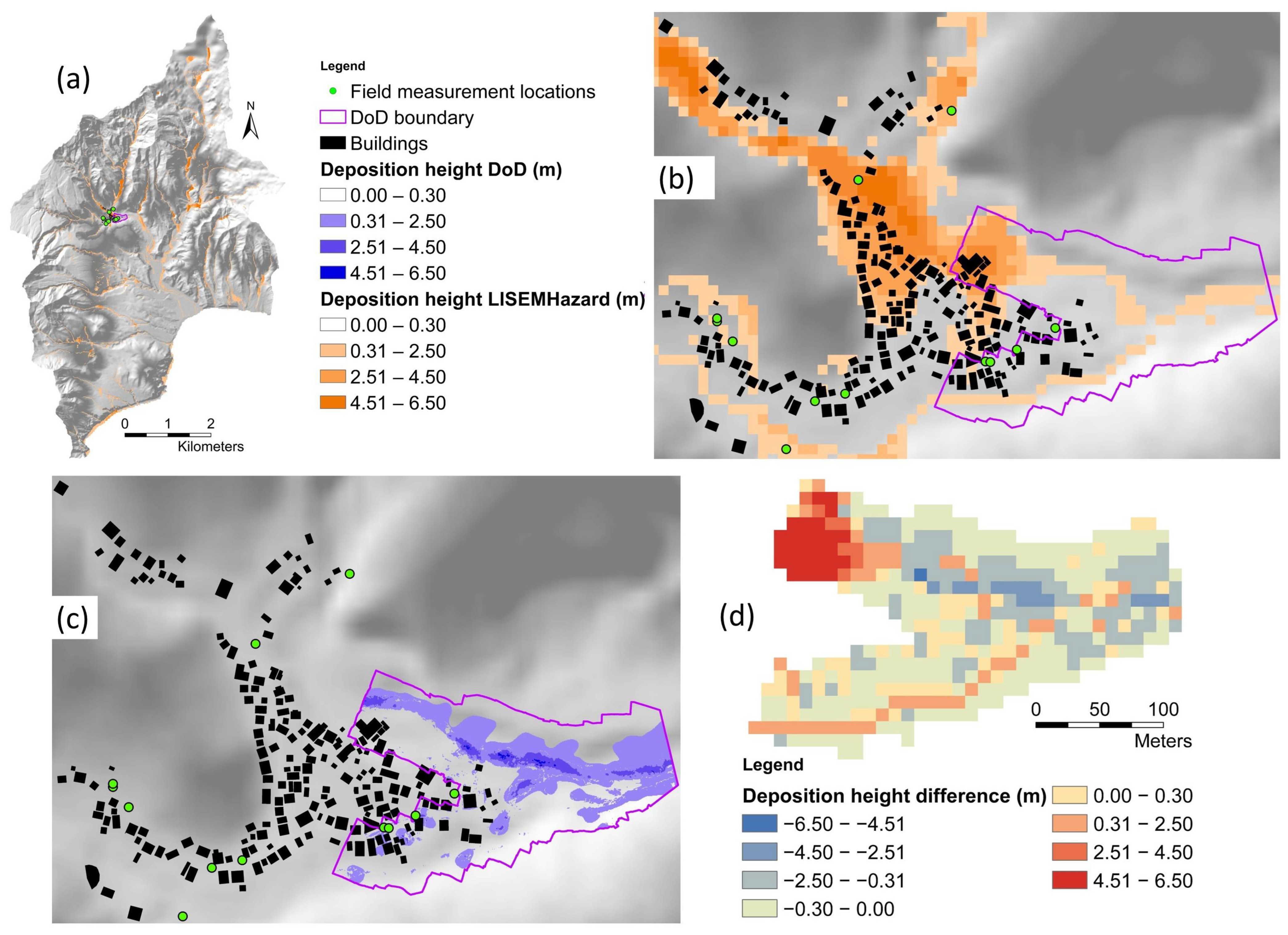
The RMSEs were calculated using the field measurement locations as check points. It should be noted that the field measurements and DoDs only cover the built-up areas of the catchments (Figure 12 and Figure 13); therefore, calculation of RMSEs was limited to these areas. For Grand Bay catchment, only three field measurements are inside DoD boundary; therefore, RMSE between modeled deposition heights and DoD was not calculated for these three locations; however, RMSE was calculated between the same two for 100 random locations within the DoD boundary.

Table 4 shows that the Cohen’s Kappa and Accuracy values are good and high respectively; however, this is due to the presence of many non-sedimented pixels that are correctly predicted by the model as non-sedimented. Sensitivity represents the probability of a positive test, conditioned on truly being positive. Sensitivity has very low values for both landslides and debris flows for both study sites, which shows poor performance of the model in predicting landslides and debris flow locations. Specificity represents the probability of a negative test, conditioned on truly being negative. Specificity has higher values compared to Sensitivity which means more non-affected pixels are correctly predicted as non-affected by the model. This can be explained by the fact that there are many pixels representing the sloping areas where no sedimentation can physically occur.

The landslide patterns and sediment deposition patterns of the two study sites are presented in Figure 8 and Figure 9. The modeled and observed landslides were compared in terms of density, total surface area, and total volume (Table 5). This shows that the modeled landslides are fewer in number, but they have similar total surface area, and a greater thickness resulting in a larger total volume. The greater thickness indicates that the strength distribution with depth in the soil is not correctly estimated. However, in reality, this is not possible. Cohesion readings can be taken at the slip surface edges, but this is far from precise. Therefore, the knowledge needed for exact locations and depth is simply missing. This is to be expected but it is also now shown by the model results.

Table 5. Comparison between the landslides indicated by the model and the inventory.

Figure 8 and Figure 9 show that the model performs poorly in predicting the locations of landslides and debris flows. The model performs better in predicting the debris flows in major channels compared to minor channels. However, the ground truth is from high resolution images where the channels show clearly the debris flows that removed vegetation and deposited debris.

Since the model is not able to predict the exact location of landslides, we compared the modeled landslides against observed ones using other approaches. From a disaster point of view, the exact locations of landslides are important when doing a detailed site investigation where buildings or infrastructure are exposed in the direct vicinity of landslides. For a larger scale hazard map, such as a national or a watershed-based hazard map, the exact location is less important than the total volume of debris and the landslide density per area of interest. We want to know to what extent the model is able to predict the debris impact in the flooded area. The first step is to look at the landslide area distribution.

The frequency density of the modeled and observed landslides was calculated and plotted against the landslide areas (Figure 10). The power-law distributions are depicted by straight lines, and the power-law exponent (slope) is given by the scaling parameter (β).

Figure 10. Frequency density of landslides indicated by the model and the inventory for (a) Coulibistrie and (b) Grand Bay catchments. The vertical dashed lines indicate the modeling grid cell size (100 m²).

For both study areas, the modeled and observed landslides show similar power-law exponent which means the model performs well in terms of predicting the size of individual landslides; however, there is a significant difference between the modeled and observed landslides of smaller size. This can be explained by the fact that the simulations are performed with 10 m spatial resolution, and it is not possible for the model to generate landslides smaller than 100 m².

Figure 10 shows that the model produced reasonably good results for landslides larger than 100 m² in Coulibistrie; however, the results for Grand Bay are less satisfactory but still acceptable. Within the model’s range of spatial resolution, the overall prediction of frequency distribution is acceptable, but prediction of precise location is not. To be able to predict smaller landslides, the model would need higher resolution of input data; however, running the model with high resolution input data requires significantly higher computing power which in practice, might not be feasible.

Slope units were digitized using the hillshading maps of the study areas and the density of landslides per slope unit was calculated. The results are presented in Figure 11. We also calculated the difference between the landslide densities indicated by the model and the inventory (model minus inventory). The observed landslides have greater densities compared to the modeled ones; however, they show similar distributions. Figure 11 shows clearly that there are areas where landslides occur but were not simulated and vice versa. The reason for this is the fact that the input maps of the geotechnical parameters (cohesion, angle of internal friction, density) do not contain sufficient details and are not representing the true spatial variation (Figure 6). Therefore, the model cannot predict the landslide pattern accurately. It is shown in Figure 6 that the input maps have large homogeneous areas. In fact, the only detailed input is the slope given by the LiDAR DTM. Hence, any other method (e.g., machine learning) would also not be able to provide accurate results using inputs of such quality.

Figure 11. (a) Density of landslides per slope unit indicated by the model for Coulibistrie. (b) Density of landslides per slope unit indicated by the inventory for Coulibistrie. (c) Difference between the landslide densities indicated by the model and the inventory (model minus inventory) for Coulibistrie; number of slope units per class is indicated between parenthesis in the legend. (d) Density of landslides per slope unit indicated by the model for Grand Bay. (e) Density of landslides per slope unit indicated by the inventory for Grand Bay. (f) Difference between the landslide densities indicated by the model and the inventory (model minus inventory) for Grand Bay; number of slope units per class is indicated between parenthesis in the legend.

LISEMHazard generates separate maps for volume of deposition on the surface and in channels. These were converted to deposition height by dividing by the cell area and were added together to obtain the total deposition. Deposition heights are displayed in Figure 12 and Figure 13. These figures show that the modeled deposition heights are overestimated compared to the observed deposition. Although the modeled and observed deposition patterns are similar, they do not occur at the same place. However, it should be noted that the deposition was not measured immediately after the event, but one year later. Hence, the measurements contain uncertainties.

Figure 12. (a) Location of 30 field measurements at Coulibistrie village shown on a hillshading map along with the buildings footprint, modeled deposition height, DoD and its boundary. (b) Zoomed view of DoD boundary with modeled deposition height. (c) Zoomed view of DoD boundary with DoD deposition height. (d) Difference between the modeled and DoD deposition heights (modeled minus DoD). As explained in Section 2.3, sediment thickness of less than 0.3m is unlikely to be visible in satellite images; therefore, this category of sediment thickness is made transparent in the DoD and LISEM deposition maps.

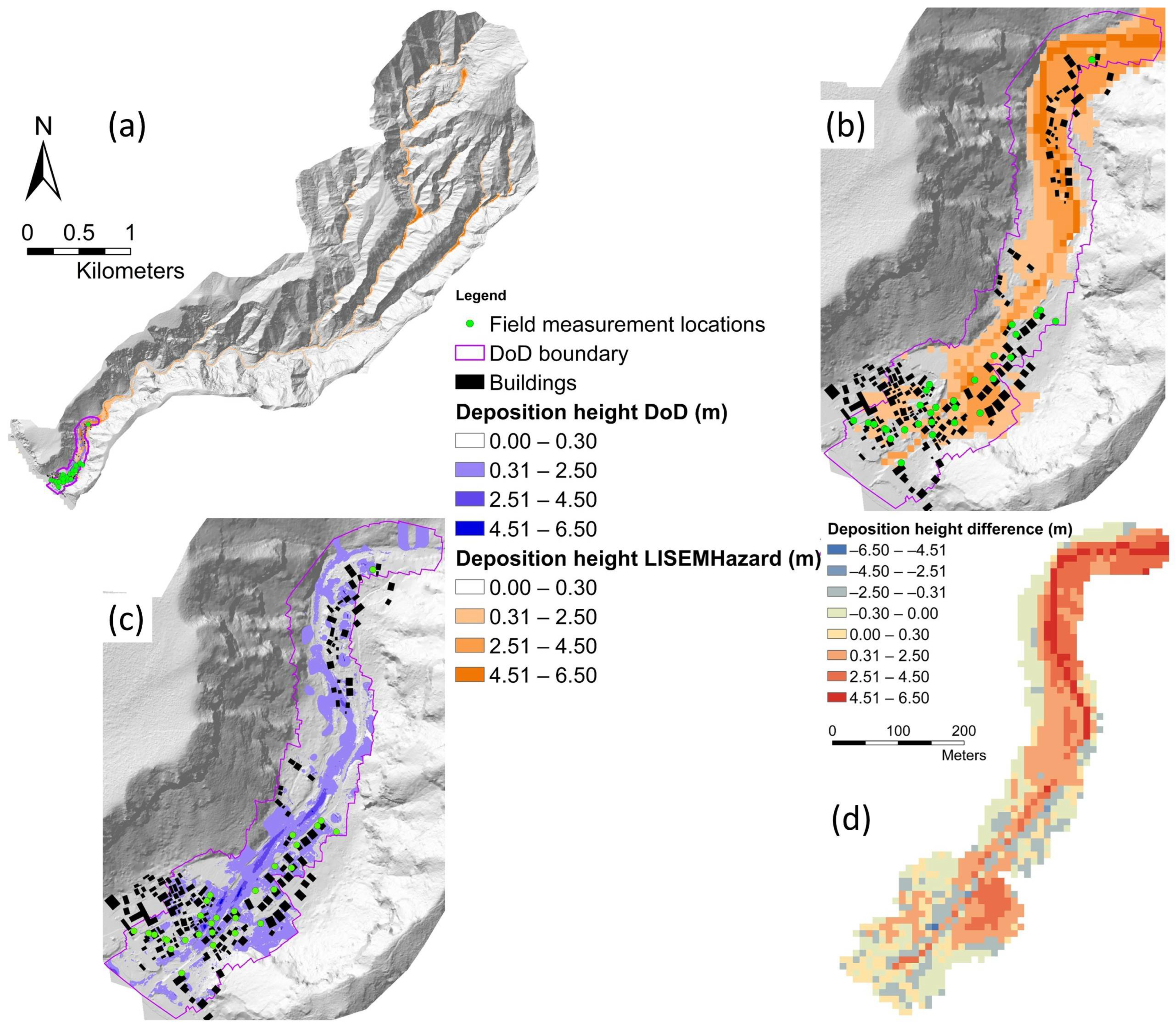
Figure 13. (a) Location of 12 field measurements at Pichelin village (in Grand Bay catchment) shown on a hillshading map along with the building footprint, modeled deposition height, DoD and its boundary. (b) Zoomed view of DoD boundary with modeled deposition height. (c) Zoomed view of DoD boundary with DoD deposition height. (d) Difference between the modeled and DoD deposition heights (modeled minus DoD). As explained in Section 2.3, sediment thickness of less than 0.3m is unlikely to be visible in satellite images; therefore, this category of sediment thickness is made transparent in the DoD and LISEM deposition maps.

3.2. Sensitivity Analysis

The absolute sediment volumes with respect to variations in input variables are presented as graphs in Figure 14. Model sensitivity was assessed as the average value of relative sensitivities for the chosen variables (Figure 15). Separate graphs were provided for sensitivity to the volume of generated, deposited, and outflowed sediments.

Figure 14. Absolute volumes of generated, deposited, and outflowed sediments with respect to variations in input variables. (a–c) Shows sensitivity for Coulibistrie. (d–f) Shows sensitivity for Grand Bay.

Figure 15. Average relative sensitivity for the generated, deposited, and outflowed sediments. (a–c) Shows sensitivity for Coulibistrie. (d–f) Shows sensitivity for Grand Bay.

The results of sensitivity analysis (Figure 14 and Figure 15) demonstrate the dominance of soil depth followed by soil cohesion in controlling the volume of sediments in all three processes of generation, deposition, and outflowing. Manning’s n and Ksat show almost no influence, while initial soil moisture and internal friction angle of soil indicate moderate influence on the volume of sediments. The negligible influence of Ksat can be explained by the dominant presence of clayey soils in both Coulibistrie and Grand Bay catchments, which leads to low Ksat values (Figure 6).

The model’s behavior is different for different input variables. Cohesion shows a strong inverse relation with the volume of sediments concerning all three processes of generation, deposition, and outflowing. Sensitivity of model increases in general when internal friction angle decreases. There is a constant increase in volume of generated and outflowed sediments with decrease in internal friction angle; however, for volume of deposited sediments, the ascending mode is reversed when the internal friction angle is decreased by more than 30 percent for Coulibistrie (Figure 14b). This can be explained by the fact that internal friction angle has a direct relation with shearing resistance of soil based on Mohr–Coulomb failure criterion [117]:

τ_{s} = c^{'} + σ . t a n (φ)

(9)

where

τ_{s}

is the shearing resistance,

c^{'}

is the summation of all cohesive terms,

σ

is the stress normal to the potential shear plane, and

φ

is the internal friction angle.

When internal friction angle is decreased, more landslides occur (Equation (A14) in Table A1 in Appendix A), but the soil shearing resistance also decreases which leads to less deposition and more outflowing.

The model has the highest sensitivity to soil depth. Deeper soils have greater weight. The greater weight of soil column can increase or decrease the slope stability depending on the slope angle of the slip surface. The component of weight perpendicular to the slope surface causes more stability, while the component of weight parallel to the surface causes more instability.

Figure 14 shows that increasing soil depth increases the sediment volume. However, similar to the case of internal friction angle, increasing soil depth by more than 40 percent causes a setback in the ascending mode of deposition volume for Coulibistrie (Figure 14b). This happens as increasing soil depth causes more failures and more sediments are generated. This leads to greater flow height and greater transport capacity which results in more outflowing and less deposition. The model is moderately sensitive to initial soil moisture. Higher values of initial soil moisture cause less absorption of water by soil, more runoff, and lower cohesion. This intensifies the transport of sediments out of catchment and results in less deposition (Figure 14b). For Grand Bay, the anomalies in deposition volume does not occur with respect to internal friction angle, soil depth, and initial soil moisture (Figure 14e). This is due to the larger size of Brand Bay catchment (34.7 km²) compared to Coulibistrie catchment (8 km²). In Grand Bay, the distance to the catchment’s outlet is considerably greater; therefore, the flowing sediments settle down inside the catchment before reaching the outlet. Ksat has a complex role. It does not show a significant sensitivity, and greater Ksat values lead to a slight increase in volume of sediments. Increasing Ksat increases absorption of water by soil and the soil column becomes heavier, which could cause more stability. At the same time, more water content increases pore pressure and leads to more instability [75]. Manning’s n has no effect on generation of sediments; however, it affects the flow velocity and transport of sediments. Decreasing Manning’s n causes higher flow velocity. Thus, more sediments will be carried out of catchment and less deposition occurs. Because the fluid has a high concentration of sediments and a higher viscosity than clear water, the effect of surface roughness on debris flow may be less than the effect of surface roughness on clear water. Hence, the effect of Mannings’ n is less than expected from the literature.

Uncertainty was assessed by calculating the standard deviation of modeled deposition heights for variations of soil depths and cohesion between −50% and +50%. These two variables were considered as the model is most sensitive to them. Figure 16 shows the deposition height map produced by the calibrated simulation (reference map), the average and the standard deviation of respective deposition height maps. The average and standard deviation maps show exaggerated deposition compared to the reference deposition map.

Figure 16. Spatial Sensitivity. (a) The reference deposition height map for Coulibistrie. (b) The average of the modeled deposition height maps for Coulibistrie. (c) The standard deviation of the modeled deposition height maps for Coulibistrie. (d) The reference deposition height map for Grand Bay. (e) The average of the modeled deposition height maps for Grand Bay. (f) The standard deviation of the modeled deposition height maps for Grand Bay.

4. Discussion

4.1. Data Uncertainty

All simulations in this study were performed at 10 m spatial resolution. Although it was possible to run simulations with higher resolutions, it was not practically feasible due to the longer simulation times. At 10 m resolution, the smallest landslide that the model can generate is 100 m² (one cell), while in reality, smaller landslides occur; therefore, at 10 m resolution, all landslides cannot be simulated. Although landslides of this size do not generate a very large amount of sediments, in cases where numerous landslides of this size have occurred but were not simulated, there will be a significant difference between the observed and simulated volume of generated sediments.

It is important to take note of the limitations regarding input data. The rainfall data came from a weather station located in Canefield airport which is approximately 15 km southeast of Coulibistrie and 10 km northwest of Grand Bay. In an ideal case, many ground stations should be available with a well spatial distribution close to the respective study site.

A high-quality pre-event DTM was not available. The DTM used for our simulations was captured at least five months after the event, which is sufficient time for changes in land topography especially during the event. The model prediction of the patterns and thickness of the landslides and deposition depends significantly on topography. Accordingly, it is likely that the model has created landslides and depositions at wrong locations. Modeling with free low-quality pre-event DTMs was also tried but discarded since the results had very poor accuracy.

SoilGrids datasets with 250 m spatial resolution were used for generating the input soil layers. This resolution is coarse enough for lots of variations in soil properties to be missed. SoilGrids products are the outputs of a system for automated global soil mapping based on state-of-the-art spatial prediction methods [101]. These predictions are based on 150,000 soil profiles used for training and a stack of 158 remote sensing-based soil covariates, which were used to fit an ensemble of machine learning methods: random forest, gradient boosting, and/or multinomial logistic regression [101]. The uncertainty levels of SoilGrids products are relatively high as the comparison to many local soil mapping projects shows high RMSE values [101].

The input landcover map was obtained from CHARIM project and it is the product of satellite imagery classification. Classification was performed with Landsat and SPOT images acquired between 1996 and 1999, which is approximately twenty years before the event. It is likely that the land cover types were changed during this period. This considerably increases the chance of simulating landslides and depositions at wrong locations.

4.2. Ground Truth Data

Different sets of data were used as ground truth data for verification of the modeling results. As indicated earlier, these datasets include the inventory of landslides and debris flows mapped by Van Westen and Zhang [91], DEMs of Difference generated by Emtehani, et al. [99], deposition height measurements in the field by Emtehani, et al. [99], and orthophotos provided by Schaefer, et al. [106].

Although these datasets are considered as ground truth, they contain some uncertainties and limitations. The inventory of landslides and debris flows were mapped using high-resolutions images (0.5 m) by image interpretation experts; however, the interpretation was carried out visually which causes uncertainty in areas where the remaining vegetation after the event spoils the visuality. Emtehani, et al. [99] have acknowledged the limitations and uncertainties associated with their DoDs, such as a more than one year gap between the event and DTM data acquisition, and the presence of vegetation, buildings, and vehicles. Field measurements of deposition height were uncertain as well due to high spatial variability of flooding and deposition level, misleading information provided by interviewees, misleading marks of building walls (flooding marks or sediment marks), a more than one year gap between the event and field data collection. The orthophotos were used to determine the flooded area boundaries. These orthophotos were captured more than four months after the event and they had a poor quality at some locations which leads to uncertainties in the digitizing the boundaries.

Collecting soil properties data (e.g., cohesion, internal friction angle, etc.) at the location of landslides is very beneficial for increasing the quality of input data for modeling. Also, measurement of landslide dimensions in the field improves the quality of observed data. The collected data needs to be well distributed over the entire catchment with a high number of data points. However, this is not feasible in Dominica due to the presence of steep slopes at high altitudes and the dense vegetation.

4.3. Model Calibration

In many runoff modeling studies, results are verified using observed discharge (e.g., De Roo, et al. [31]; Kværnø and Stolte [21], Rickenmann, et al. [32];). In this research, since no observed discharge data was available; model calibration was performed based on the observed landslide and deposition heights and patterns.

It should be noted that if the calibration is based on one parameter only (e.g., landslide patterns), no logical results will be produced. For instance, if we focus on generating the correct height and pattern of sediment deposition, we would need to simulate an exaggerated number of landslides. On the other hand, if we only focus on generating the correct volume and pattern of landslides, we will get unrealistic deposition. Therefore, it is crucial to calibrate the model in such a way that a logical balance is maintained between all different processes. This is, in fact, a problem of the model: uncertainty in entrainment in the riverbeds (both in observations and in the model) and the absence of simulated landslides smaller than 100 m² contributing to a wrong sediment volume, which then needs to be compensated by simulating more larger landslides. The transport process between landslides and the deposited sediments downstream greatly depends on channel characteristics, which are determined in this study completely based on estimation.

Initial simulations did not produce enough deposition at the catchments’ downstream part; therefore, the model was calibrated so that landslides were intensified, and more sediments were produced but unrealistic landslides were avoided. Sediment deposition boundaries were digitized using orthophotos (Figure 17). It indicates that the modeled deposition near the catchment outlet is less than observed deposition. This is despite the fact that the modeled landslides have greater total volume compared to the observed landslides as indicated by Table 5. This shows that the generated sediments (by landslides) in LISEMHazard do not travel very far from their sources and deposition is more a local effect. This can be considered as one of the limitations of this model. The model characterizes the sediment content with two grain sizes which affect the flow dynamics, but the reality is more complex.

Figure 17. Modeled sediment deposition shown on an orthophotos of Coulibistrie (a) and Pichelin (b) villages. The orthophotos do not cover the entire catchments. The observed sediment deposition boundary is indicated by the red polygon.

4.4. Accuracy Assessment

Accuracy of the modeling results was assessed with regards to sediment source and deposition processes. The first two RMSEs for deposition heights (at field measurements locations) for Coulibistrie show similar values (0.75 m and 0.72 m) (Table 4). These values cannot be considered very high accuracies, but they are reasonably good, especially if the difference between DoDs and modeled maps in terms of spatial resolution (0.5m and 10m respectively) is taken into consideration. The calculated RMSEs for Grand Bay are lower accuracies compared to Coulibistrie. The first RMSE is based on 12 check points in Pichelin (Grand Bay), which is not enough for a reliable accuracy assessment. Also, the field measurements in Pichelin were mostly based on interviews with local residents and they contain a higher level of uncertainty compared to field measurements in Coulibistrie, which were mostly based on direct field observations. RMSEs were also calculated based on 100 random points for both Coulibistrie and Grand Bay, but they have significantly higher values (2.09 m and 2.24 m). This can be explained by the fact that the field measurements took place at locations where both DoD and the modeled deposition height have non-zero values; however, many of the random points are located at places where DoD has zero value, but the modeled deposition has non-zero value. This indicates that the model does not predict the exact location of sediment depositions.

Analysis of slope failures indicates that although the model produces fewer landslides, the total volume of modeled landslides is significantly larger than that of observed landslides (Table 5). However, the difference between the total surface area of modeled and observed landslides is small. The surface area of modeled landslides was used to calculate the volumes with the empirical approach (Equation (7)). This returned volumes much closer to the observed volumes. This shows that the model overestimates the landslides’ depth.

The model cannot produce landslides smaller than a cell area. Therefore, the modeled landslides have a minimum surface area of 100 m², while the inventory contains a considerable number of landslides with small surface area (Figure 10). Also, the model predicts many landslides at wrong locations (Figure 8 and Figure 9). This is partially caused by the input soil depth map which itself is a product of modeling with a medium level of uncertainty [103]. Nevertheless, the predicted and observed landslides show similar frequency density distributions with similar power-law exponent values (Figure 10). Density of landslides per slope units reaffirms that the model is not capable of predicting the correct locations of landslides, yet the general patterns of modeled landslide densities are very similar to the observed ones. However, prediction of the exact location of landslides and their patterns is not very important in practice, rather reasonable estimation of the total volume of sediments (to be removed) is crucial.

Debris flows are depicted in Figure 8 and Figure 9. There is good agreement between modeled and observed debris flows in the main channels, while there is no or slight agreement in narrow channels. This can be a matter of debris flows mapping with satellite imagery. It is very likely that shallower flows which occurred on steeper slopes were not visible in satellite images due to presence of vegetation and were not included in the inventory.

4.5. Sensitivity Analysis

The model is most sensitive to soil depth and cohesion for all three processes of sediment generation, transport, and outflowing. The model shows no or lower level of sensitivity to the other variables considered in this study. Soil depth and cohesion have high spatial variability and are difficult to determine. There are lots of studies focused on soil depth estimation and many of them are based on regression analysis and spatial interpolation (Dietrich, Reiss, Hsu and Montgomery [45], Tesfa, et al. [118], Sarkar, et al. [119], Liao, et al. [120], Horst-Heinen, et al. [121]). Also, values of soil cohesion can be obtained from the literature for different soil types (US Navy [122], SN [123], Patil, et al. [124]). Cohesion can be measured in the field as well with shear vane test; however, this cannot be done for the subsoil layer. The uncertainty within each of these approaches limits the reliability of the relative model inputs. This results in a high level of uncertainty in simulation results as the model is very sensitive to these two variables [31,113,125]. Sensitivity of LISEMHazard was assessed by de Vugt [26]. Same as the findings of our research, they found that LISEMHazard is most sensitive to soil depth, cohesion, internal friction angle, and initial soil moisture. However, de Vugt [26] assessed the sensitivity of the model with respect to measured discharge, while in our study the volume of sediments was taken into account.

Sensitivity analysis is useful for assessing the behavior of the model with regards to individual input variables; however, the modeling outputs are a combination of all inputs. Therefore, we calculated the average and standard deviation of all results for variations of the two variables to which the model is most sensitive. The average and standard deviation maps show exaggerated patterns and heights. Variations in soil depth and cohesion lead to a vast range of sediment deposition heights ranging from zero to unrealistically large values. This leads to large values in the average and standard deviation maps.

5. Conclusions

After an event deposition is a mixture of sediments, rocks and boulders, tree logs, and other debris [126]; however, the model does not indicate the particle size of deposited material. This information is crucial for estimation of total loss as the cleaning cost for different types of materials is not identical. The presence of large boulders and tree logs in debris flows causes additional losses as they quickly fill the channels and block the culverts and spaces below bridges, causing intensified flooding and spread of debris materials in larger areas. The sediment transport of the model is related to the grainsizes, and since these are simplified, the link between source areas and downstream deposition areas cannot be calibrated well with detailed observations of the riverbed before an event. This is not possible in reality.

Soil depth and cohesion are the two variables that need to be investigated with great care as they have a significant impact on the modeling results. It happens rarely that a high-quality dataset (especially soil depth) is available for a specific site. Collecting ground truth data for increasing the accuracy of input data is very helpful. Also, large number of field measurements of sediment deposition height and patterns with good distribution over the entire catchment area are useful for model calibration and accuracy assessment of the results.

Quantification of sediment deposition as a hazard intensity by modeling the landslides upstream and the sediment transport process is a very complicated task. Transport of sediments occurs from landslides (as source of sediments) by flooding and debris flow with a variety of grainsizes and presence of other materials (e.g., tree logs, cars, etc.). In addition to that, transport of some sediments does not end downstream and in some cases, sediments are transported further downstream (out of the catchment) or to the sea. Therefore, the whole process is associated with a lot of uncertainties and limitations for both modeling and field measuring. Nevertheless, modeling is the most feasible method for spatial estimation of deposition heights and prediction of the risk of sediments under future scenarios. Insightful calibration and validation are of vital importance for achieving reasonable results.

Given the significance of terrain representation and the sensitivity of the modeling results to soil depth and cohesion, improving the quality and spatial consistency of the input datasets is essential for enhancing model performance. Future work should, therefore, focus on utilizing higher-quality input datasets, which would allow a more robust evaluation of the model’s predictive capability under improved data conditions. The outcomes of this research can be used for risk assessment of sediment deposition events. It is useful for evaluation of the damage to buildings’ structure and contents, and for estimation of sediment cleanup costs.

Author Contributions

Conceptualization, S.E., V.J., C.v.W. and B.v.d.B.; methodology, S.E., V.J., C.v.W. and B.v.d.B.; software, S.E., V.J., C.v.W. and B.v.d.B.; validation, S.E., V.J., C.v.W. and B.v.d.B.; formal analysis, S.E., V.J., C.v.W. and B.v.d.B.; investigation, S.E.,V.J., C.v.W. and B.v.d.B.; data curation, S.E., V.J., C.v.W. and B.v.d.B.; writing—original draft preparation, S.E.; writing—review and editing, S.E., V.J., C.v.W. and B.v.d.B.; visualization, S.E. All authors have read and agreed to the published version of the manuscript.

Funding

This research has received funding from the European Union’s Horizon 2021 PARATUS project under Grant Agreement No. 101073954.

Data Availability Statement

The original contributions presented in this study are included in the article. Further inquiries can be directed to the corresponding author.

Acknowledgments

The authors would like to acknowledge the support of the PARATUS project.

Conflicts of Interest

The authors declare no conflicts of interest.

Appendix A

The governing equations of LISEMHazard and their variables are presented in this Appendix.

Table A1. The governing equations of LISEMHazard (Bout, et al. [74]; Bout and Jetten [97]).

Process	Equation		References
Interception	$I_{c} = S_{m a x} (1 - e^{- k \frac{P_{c u m}}{S_{m a x}}})$	(A1)	Aston [127]
Infiltration (Green & Amp)	$f = - K_{s} (ψ \frac{θ_{s} - θ_{i}}{F} + 1)$	(A2)	Kutílek and Nielsen [128]
Surface flow (dynamic flow)	$\frac{\partial h}{\partial t} + \frac{\partial (h u_{x})}{\partial x} + \frac{\partial (h u_{y})}{\partial y} = q - I$	(A3)	de Saint Venant [129]; Delestre, et al. [98]
	$\frac{\partial h u_{x}}{\partial t} + \frac{\partial (h u_{x}^{2} + \frac{1}{2} g h^{2})}{\partial x} + \frac{\partial (h u_{x} u_{y})}{\partial y} = g h (S_{x} - S_{f, x})$	(A4)
	$\frac{\partial h u_{y}}{\partial t} + \frac{\partial (h u_{x} u_{y})}{\partial y} + \frac{\partial (h u_{y}^{2} + \frac{1}{2} g h^{2})}{\partial x} = g h (S_{y} - S_{f, y})$	(A5)
Splash detachment	${d e p}_{s p l a s h} = (\frac{2.82}{A_{s}} K_{e} e^{(- 1.48 h)} + 2.96) P_{h} \frac{A}{d t}$	(A6)	De Roo, et al. [31]
Stream power and transport capacity	$ω = V S$	(A7)	Govers [130]
	$T = c {(T C - 0.004)}^{d}$	(A8)
	$c = {(\frac{D 50 + 5}{0.32})}^{- 0.6}$	(A9)
	$d = {(\frac{D 50 + 5}{300})}^{0.25}$	(A10)
Erosion & deposition	$d e p = w_{s} B \min (0.0, (T - C))$	(A11)	Morgan, et al. [54]
Erosion & deposition	$d e t = γ w_{s} B m a x (0.0, (T - C))$	(A12)	Morgan, et al. [54]
Sediment transport	$\frac{d S}{d t} + \frac{d (Q_{x} C)}{d x} + \frac{d (Q_{y} C)}{d y} = d e p - d e t$	(A13)	Bout, et al. [74]
Slope stability	$S F = \frac{c^{'} + c + ((γ - m γ_{w}) z + m γ_{w} z) \cos {(β)}^{2} t a n (\emptyset^{'})}{((γ - m γ_{w}) z) \sin (β) c o s (β)}$	(A14)	Kuriakose, et al. [103]; Kuriakose, et al. [104]
Debris flow	$S_{x, s} = α_{s} (g (\partial h / \partial x) - (u_{s} / \| \vec{u_{s}} \|) \cdot t a n (ρ P_{β, s}) - e P_{β, s} (\partial h / \partial x) - ε α_{s} γ P_{β, s} (\partial h / \partial x + \partial b / \partial x) + C^{DG} (u_{r} - u_{s}) \| \vec{u_{r}} - \vec{u_{s}} \|^{j - 1})$	(A15)	van den Bout [131]
	$S_{γ, s} = α_{s} (g (\partial h / \partial y) - (v_{s} / \| \vec{u_{s}} \|) \cdot t a n (ρ P_{β, s}) - e P_{β, s} (\partial h / \partial y) - ε α_{s} γ P_{β, s} (\partial h / \partial y + \partial b / \partial y) + C^{DG} (v_{r} - v_{s}) \| \vec{u_{r}} - \vec{u_{s}} \|^{j - 1})$	(A16)
	$S_{x, s} = α_{f} (g (\partial h / \partial x) - [(1 / h) \cdot \partial / \partial x (h^{2} / 2 \cdot P_{β, r}) + P_{β, r} \cdot \partial h / \partial x - (1 / (α_{f} N^{R})) (2 \partial^{2} u_{r} / \partial x^{2} + \partial^{2} v_{r} / \partial x \partial y - χ u_{r} / (h^{2} + 1))])$ $- (1 / (α_{f} N^{R})) (\partial / \partial x (\partial u_{r} / \partial x (u_{r} - u_{s})) + (\partial / \partial x (\partial v_{r} / \partial_{x} (v_{r} - v_{s})))$ $- ξ α_{f} (v_{r} - v_{s}) \cdot \partial / \partial x (u_{r} / h) - (1 / γ) C^{DG} (u_{r} - u_{s}) \| \vec{u_{r}} - \vec{u_{s}} \|^{j - 1}$	(A17)
	$S_{γ, s} = α_{f} (g (\partial h / \partial y) - [(1 / h) \cdot \partial / \partial y (h^{2} / 2 \cdot P_{β, r}) + P_{β, r} \cdot \partial h / \partial y - (1 / (α_{f} N_{R})) (2 \partial^{2} v_{r} / \partial y^{2} + \partial^{2} u_{r} / \partial x \partial y - χ v_{r} / (h^{2} + 1))])$ $- (1 / (α_{f} N_{R})) (\partial / \partial y (\partial u_{r} / \partial y (u_{r} - u_{s})) + (\partial / \partial y (\partial v_{r} / \partial y (v_{r} - v_{s})))$ $- ξ α_{f} (u_{r} - u_{s}) \cdot \partial / \partial y (v_{r} / h) - (1 / γ) C^{DG} (v_{r} - v_{s}) \| \vec{u_{r}} - \vec{u_{s}} \|^{j - 1}$	(A18)

Table A2. Variables of the LISEMHazard governing equations.

Variable	Description	Unit
I_c	Total intercepted storage at a given time	mm
S_max	Maximum canopy storage	mm
P_cum	Total precipitation	mm
k	Parameter related to canopy openness	-
K_s	Saturated hydraulic conductivity	m s⁻¹
Ψ	Matric pressure at the wetting front	m
Θ_s	Porosity	m³ m⁻³
Θ_i	Initial soil moisture content	m³ m⁻³
F	Cumulative infiltrated water	m
h	Flow height	m
u	Flow velocity	m s⁻¹
q	Discharge flux	m s⁻¹
I	Infiltration rate	m s⁻¹
S_x & S_y	Slope in x and y directions	m m⁻¹
S_f,x & S_f,y	Friction slope terms in the x and y directions (estimated by Pudasaini).	m m⁻¹
Dep_splash	Splash deposition rate	kg m⁻² s⁻¹
A_s	Aggregate stability, median number of drops to decrease the aggregate mass by 50%	-
K_e	Kinetic energy of the rainfall	J m⁻² m m⁻¹
P_h	Rainfall or throughfall	mm
A	Surface area where the splash detachment takes place	m²
Dep (Equation (A11))	Deposition	kg m⁻² s⁻¹
Det (Equation (A12))	Detachment	kg m⁻² s⁻¹
w_s	Settling velocity	m s⁻¹
B	Flow width	m
T	Transport capacity	kg m⁻³
C	Sediment concentration	kg m⁻³
γ	Erosion efficiency coefficient	-
S	Sediment load	kg
C	Sediment concentration	kg m⁻³
Q	Discharge	m³ s⁻¹
dep (Equation (A13))	Deposition	kg s⁻¹
det (Equation (A13))	Detachment	kg s⁻¹
SF	Safety factor	-
$γ$ (Equation (A14))	Soil density	kg m⁻³
$γ_{w}$	Water density	kg m⁻³
$z$	Soil depth	m
$β$	Soil section slope	-
$c$	Soil cohesion	kPa
$c^{'}$	Soil apparent cohesion	kPa
$\emptyset^{'}$	Soil internal friction angle	-
D₅₀	Median grain diameter	µm
ω	Stream power	m s⁻¹
a_s & a_f	Volume fraction for solid and fluid phases	-
P_b	Pressure at the base surface	kg m⁻¹ s⁻²
b	Basal surface of the flow	m
N_R	Reynolds number	-
N_RA	Quasi-Reynolds number	-
C_DG	Drag coefficient	-
ρ_f	Density of the fluid	kg m⁻³
ρ_s	Density of the solids	kg m⁻³
$γ$ (Equation (A15))	Density ratio between the fluid and solid phase	-
χ	Vertical shearing of fluid velocity	m s⁻¹
ε	Aspect ratio of the model	-
ξ	Vertical distribution of a_s	m⁻¹

References

Merz, B.; Kreibich, H.; Schwarze, R.; Thieken, A. Review article “Assessment of economic flood damage”. Nat. Hazards Earth Syst. Sci. 2010, 10, 1697–1724. [Google Scholar] [CrossRef] [Scilit]
Bohner, A.; Winter, S.; Kraml, B.; Holzner, W. Destructive and constructive effects of mudflows–primary succession and success of pasture regeneration in the nature park Sölktäler (Styria, Austria). In Proceedings of the 5th Symposium for Research in Protected Areas, Mittersill, Austria, 10–12 June 2013; pp. 10–12. [Google Scholar]
Kim, H.Y.; Julien, P.Y. Hydraulic thresholds to mitigate sedimentation problems at Sangju Weir, South Korea. J. Hydraul. Eng. 2018, 144, 05018005. [Google Scholar] [CrossRef] [Scilit]
Vázquez-Tarrío, D.; Ruiz-Villanueva, V.; Garrote, J.; Benito, G.; Calle, M.; Lucía, A.; Díez-Herrero, A. Effects of sediment transport on flood hazards: Lessons learned and remaining challenges. Geomorphology 2024, 446, 108976. [Google Scholar] [CrossRef] [Scilit]
Verstraeten, G.; Poesen, J. The nature of small-scale flooding, muddy floods and retention pond sedimentation in central Belgium. Geomorphology 1999, 29, 275–292. [Google Scholar] [CrossRef] [Scilit]
Boardman, J.; Evans, R.; Ford, J. Muddy floods on the South Downs, southern England: Problem and responses. Environ. Sci. Policy 2003, 6, 69–83. [Google Scholar] [CrossRef] [Scilit]
Dietrich, W.E. Settling velocity of natural particles. Water Resour. Res. 1982, 18, 1615–1626. [Google Scholar] [CrossRef] [Scilit]
Zachar, D. Soil Erosion; Elsevier: Amsterdam, The Netherlands, 2011; Volume 10. [Google Scholar]
Cerdan, O.; Govers, G.; Le Bissonnais, Y.; Van Oost, K.; Poesen, J.; Saby, N.; Gobin, A.; Vacca, A.; Quinton, J.; Auerswald, K. Rates and spatial variations of soil erosion in Europe: A study based on erosion plot data. Geomorphology 2010, 122, 167–177. [Google Scholar] [CrossRef] [Scilit]
García-Ruiz, J.M. The effects of land uses on soil erosion in Spain: A review. Catena 2010, 81, 1–11. [Google Scholar] [CrossRef] [Scilit]
Borrelli, P.; Robinson, D.A.; Fleischer, L.R.; Lugato, E.; Ballabio, C.; Alewell, C.; Meusburger, K.; Modugno, S.; Schütt, B.; Ferro, V. An assessment of the global impact of 21st century land use change on soil erosion. Nat. Commun. 2017, 8, 2013. [Google Scholar] [CrossRef] [Scilit]
Andualem, T.G.; Hewa, G.A.; Myers, B.R.; Peters, S.; Boland, J.J.L. Erosion and sediment transport modeling: A systematic review. Land 2023, 12, 1396. [Google Scholar] [CrossRef] [Scilit]
Luo, H.; Fan, R.; Wang, H.; Zhang, L. Physics of building vulnerability to debris flows, floods and earth flows. Eng. Geol. 2020, 271, 105611. [Google Scholar] [CrossRef] [Scilit]
Quan Luna, B.; Blahut, J.; Van Westen, C.; Sterlacchini, S.; van Asch, T.W.; Akbas, S. The application of numerical debris flow modelling for the generation of physical vulnerability curves. Nat. Hazards Earth Syst. Sci. 2011, 11, 2047–2060. [Google Scholar] [CrossRef] [Scilit]
Jakob, M.; Stein, D.; Ulmi, M. Vulnerability of buildings to debris flow impact. Nat. Hazards 2012, 60, 241–261. [Google Scholar] [CrossRef] [Scilit]
Dai, Z.; Huang, Y.; Cheng, H.; Xu, Q. SPH model for fluid–structure interaction and its application to debris flow impact estimation. Landslides 2017, 14, 917–928. [Google Scholar] [CrossRef] [Scilit]
Cui, P.; Zeng, C.; Lei, Y. Experimental analysis on the impact force of viscous debris flow. Earth Surf. Process. Landf. 2015, 40, 1644–1655. [Google Scholar] [CrossRef] [Scilit]
Viccione, G.; Ferlisi, S.; Marra, E. A numerical investigation of the interaction between debris flows and defense barriers. In Proceedings of the 8th International Conference on Environmental and Geological Science and Engineering (EG’15), Salerno, Italy, 27–29 June 2015; pp. 27–29. [Google Scholar]
Chen, Y.; Lin, C.; Reijinders, J.; Stolte, J. Calibration and validation of limburg soil erosion model (LISEM) for the small catchment in the purple hilly masses of Sichuan basin. Southwest China J. Agric. Sci. 2007, 20, 669–675. [Google Scholar]
Baartman, J.; Jetten, V.; Ritsema, C.; De Vente, J. Exploring effects of rainfall intensity and duration on soil erosion at the catchment scale using OpenLISEM. In EGU General Assembly Conference Abstracts; Geophysical Research Abstracts: Katlenburg-Lindau, Germany, 2012; p. 651. [Google Scholar]
Kværnø, S.H.; Stolte, J. Effects of soil physical data sources on discharge and soil loss simulated by the LISEM model. Catena 2012, 97, 137–149. [Google Scholar] [CrossRef] [Scilit]
Rahmati, M.; Neyshabouri, M.R.; Fakherifard, A.; Oskouei, M.M.; Ahmadi, A.; Sheikh, J.V. Rainfall-runoff prediction using LISEM model in Lighvan watershed, North West of Iran. Tech. J. Eng. Appl. Sci. 2013, 3, 1893–1901. [Google Scholar]
Clutario, M.V.A.; David, C.P.C. Event-based Soil Erosion Estimation in a Tropical Watershed. Int. J. For. Soil Eros. 2014, 4, 51. [Google Scholar]
Ferket, B.; Van De Broek, M.; Van Hoestenberghe, T.; Degerickx, J.; De Sutter, R.; Govers, G.; Dezillie, N.; Deproost, P. Erosion modelling towards, and sediment transport modelling in unnavigable watercourses in Flanders, Belgium. Proc. Int. Assoc. Hydrol. Sci. 2015, 367, 349–356. [Google Scholar] [CrossRef] [Scilit]
Nurritasari, F.A.; Sudibyakto, S.; Jetten, V.G. OpenLISEM Flash Flood Modelling Application in Logung Sub-Catchment, Central Java. Indones. J. Geogr. 2015, 47, 132–141. [Google Scholar] [CrossRef] [Scilit]
de Vugt, L.C. Mapping and Modelling of Landslide and Flood Hazards on St. Eustatius with openLISEM. Master’s Thesis, Utrecht Universit, Utrecht, The Netherlands, 2018. [Google Scholar]
Xiao, Y. Analyzing the Predictive Capacity of a Physically-Based Debris Flow Model: A Case Study for Debris Flow in the Post-2008 Wenchuan Earthquake Area. Master’s Thesis, University of Twente, Enschede, The Netherlands, 2020. [Google Scholar]
van den Bout, B.; Tang, C.; van Westen, C.; Jetten, V. Physically-based modelling of co-seismic landslide, debris flow and flood cascade. Nat. Hazards Earth Syst. Sci. Discuss. 2022, 22, 3183–3209. [Google Scholar] [CrossRef] [Scilit]
Mergili, M.; Emmer, A.; Juřicová, A.; Cochachin, A.; Fischer, J.T.; Huggel, C.; Pudasaini, S.P. How well can we simulate complex hydro-geomorphic process chains? The 2012 multi-lake outburst flood in the Santa Cruz Valley (Cordillera Blanca, Perú). Earth Surf. Process. Landf. 2018, 43, 1373–1389. [Google Scholar] [CrossRef] [Scilit] [PubMed]
Takken, I.; Beuselinck, L.; Nachtergaele, J.; Govers, G.; Poesen, J.; Degraer, G. Spatial evaluation of a physically-based distributed erosion model (LISEM). Catena 1999, 37, 431–447. [Google Scholar] [CrossRef] [Scilit]
De Roo, A.; Wesseling, C.; Ritsema, C. LISEM: A single-event physically based hydrological and soil erosion model for drainage basins. I: Theory, input and output. Hydrol. Process. 1996, 10, 1107–1117. [Google Scholar]
Rickenmann, D.; Laigle, D.; McArdell, B.; Hübl, J. Comparison of 2D debris-flow simulation models with field events. Comput. Geosci. 2006, 10, 241–264. [Google Scholar] [CrossRef] [Scilit]
Schraml, K.; Thomschitz, B.; McArdell, B.; Graf, C.; Kaitna, R. Modeling debris-flow runout patterns on two alpine fans with different dynamic simulation models. Nat. Hazards Earth Syst. Sci. 2015, 15, 1483–1492. [Google Scholar] [CrossRef] [Scilit]
Frank, F.; McArdell, B.W.; Oggier, N.; Baer, P.; Christen, M.; Vieli, A. Debris-flow modeling at Meretschibach and Bondasca catchments, Switzerland: Sensitivity testing of field-data-based entrainment model. Nat. Hazards Earth Syst. Sci. 2017, 17, 801–815. [Google Scholar] [CrossRef] [Scilit]
Zegers, G.; Mendoza, P.A.; Garces, A.; Montserrat, S. Sensitivity and identifiability of rheological parameters in debris flow modeling. Nat. Hazards Earth Syst. Sci. 2020, 20, 1919–1930. [Google Scholar] [CrossRef] [Scilit]
Defersha, M.B.; Melesse, A.M.; McClain, M.E. Watershed scale application of WEPP and EROSION 3D models for assessment of potential sediment source areas and runoff flux in the Mara River Basin, Kenya. Catena 2012, 95, 63–72. [Google Scholar] [CrossRef] [Scilit]
Schmidt, J.; Werner, M.; Michael, A. Application of the EROSION 3D model to the CATSOP watershed, The Netherlands. Catena 1999, 37, 449–456. [Google Scholar] [CrossRef] [Scilit]
Schindewolf, M.; Schmidt, J. Parameterization of the EROSION 2D/3D soil erosion model using a small-scale rainfall simulator and upstream runoff simulation. Catena 2012, 91, 47–55. [Google Scholar] [CrossRef] [Scilit]
Hairsine, P.; Rose, C. Modeling water erosion due to overland flow using physical principles: 1. Sheet flow. Water Resour. Res. 1992, 28, 237–243. [Google Scholar] [CrossRef] [Scilit]
Hairsine, P.; Sander, G.; Rose, C.; Parlange, J.-Y.; Hogarth, W.; Lisle, I.; Rouhipour, H. Unsteady soil erosion due to rainfall impact: A model of sediment sorting on the hillslope. J. Hydrol. 1999, 220, 115–128. [Google Scholar] [CrossRef] [Scilit]
Dietrich, W.E.; Wilson, C.J.; Montgomery, D.R.; McKean, J. Analysis of erosion thresholds, channel networks, and landscape morphology using a digital terrain model. J. Geol. 1993, 101, 259–278. [Google Scholar] [CrossRef] [Scilit]
Montgomery, D.R.; Dietrich, W.E. A physically based model for the topographic control on shallow landsliding. Water Resour. Res. 1994, 30, 1153–1171. [Google Scholar] [CrossRef] [Scilit]
Pack, R.T.; Tarboton, D.G.; Goodwin, C.N. The SINMAP approach to terrain stability mapping. In Proceedings of the 8th Congress of the International Association of Engineering Geology, Vancouver, BC, Canada, 21–25 September 1998. [Google Scholar]
Dietrich, W.E.; Wilson, C.J.; Montgomery, D.R.; McKean, J.; Bauer, R. Erosion thresholds and land surface morphology. Geology 1992, 20, 675–679. [Google Scholar] [CrossRef] [Scilit]
Dietrich, W.E.; Reiss, R.; Hsu, M.L.; Montgomery, D.R. A process-based model for colluvial soil depth and shallow landsliding using digital elevation data. Hydrol. Process. 1995, 9, 383–400. [Google Scholar] [CrossRef] [Scilit]
Deltares. Delft3D-FLOW: Simulation of Multi-Dimensional Hydrodynamic Flows and Transport Phenomena, Including Sediments; Deltares: Delft, The Netherlands, 2024. [Google Scholar]
Fauzah, S.; Tarya, A.; Ningsih, N.S. Three-Dimensional Numerical Modelling of Tidal Current in Balikpapan Bay Using Delft 3D. IOP Conf. Ser. Earth Environ. Sci. 2021, 925, 012051. [Google Scholar] [CrossRef] [Scilit]
Theol, S.A.; Charlotte de Fraiture, F. Understanding Cohesive Sediments Behaviour In Irrigation Canals Using Delft 3d Model Simulation. In Proceedings of the 2nd World Irrigation Forum, Chiang Mai, Thailan, 6–8 November 2016. [Google Scholar]
Betrie, G.; Van Griensven, A.; Mohamed, Y.; Popescu, I.; Mynett, A.; Hummel, S. Linking SWAT and SOBEK using open modeling interface (OPENMI) for sediment transport simulation in the Blue Nile River basin. Trans. ASABE 2011, 54, 1749–1757. [Google Scholar] [CrossRef] [Scilit]
Deltares SUM. Hydrodynamics, Rainfall Runoff and Real Time Control; Deltares: Delft, The Netherlands, 2015. [Google Scholar]
Ji, Z.; de VRIEND, H.; Hu, C. Application of SOBEK model in the Yellow River estuary. In Proceedings of the International Conference on Estuaries and Coasts, Hangzhou, China, 9–11 November 2003; Available online: https://d1wqtxts1xzle7.cloudfront.net/47048732/APPLICATION_OF_SOBEK_MODEL_IN_THE_YELLOW20160706-22547-1x44ibb-libre.pdf?1467799283=&response-content-disposition=inline%3B+filename%3DApplication_of_Sobek_Model_in_the_Yellow.pdf&Expires=1771191329&Signature=cpY5TL1JcqRnk3T94UJ9NHVjPWk162h276xhmYCsFFDAGB~f6FuO2uSUF3t3Cx7WuYDrkWh5HgX2erOen-uVoOvXTlQNkRmIOqzxaAUj56p8gADu0u9DE8NdMFAQNV4CGSz4AbctuUfxK8oca~OXiVoUzKKQ8Jdtxr~Fvy7TPziQqSmerrSaT-u33SAHjmug8HbSZUGvAH3PnZ1-aUSXxAGs5r4SutUMeaQVDwXKdP0i7HhbLy82uy6xi84R7yEccWYCiW~8fc175lGltELvDwrhtsrMt4dDkaPTo-~xfFbL9xEtL- (accessed on 1 January 2020).
Flanagan, D.; Frankenberger, J.; Ascough, J., II. WEPP: Model use, calibration, and validation. Trans. ASABE 2012, 55, 1463–1477. [Google Scholar] [CrossRef] [Scilit]
USDA Agricultural Research Service (ARS). WEPP User Requirements Document; National Soil Erosion Research Laboratory: West Lafayette, IN, USA, 1987. Available online: https://www.ars.usda.gov/ARSUserFiles/50201000/WEPP/docs/wepp-user-requirements.pdf (accessed on 10 February 2026).
Morgan, R.; Quinton, J.; Smith, R.; Govers, G.; Poesen, J.; Auerswald, K.; Chisci, G.; Torri, D.; Styczen, M. The European Soil Erosion Model (EUROSEM): A dynamic approach for predicting sediment transport from fields and small catchments. Earth Surf. Process. Landf. J. Br. Geomorphol. Group 1998, 23, 527–544. [Google Scholar] [CrossRef] [Scilit]
Morgan, R.; Quinton, J.; Smith, R.; Govers, G.; Poesen, J.; Auerswald, K.; Chisci, G.; Torri, D.; Styczen, M.; Folly, A. The European Soil Erosion Model (EUROSEM): Documentation and User Guide; Silsoe College, Cranfield University: Bedford, UK, 1998; Volume 89. [Google Scholar]
Nakatani, K.; Satofuka, Y.; Mizuyama, T. Development Ofkanako’, a Wide Use Debris Flow Simulator Equipped with Gui. In Proceedings of the Congress-International Association For Hydraulic Research, Venice, Italy, 1–6 July 2007; p. 430. [Google Scholar]
Nakatani, K.; Wada, T.; Satofuka, Y.; Mizuyama, T. Development of “Kanako 2D (Ver. 2.00),” a user-friendly one-and two-dimensional debris flow simulator equipped with a graphical user interface. Int. J. Eros. Control Eng. 2008, 1, 62–72. [Google Scholar] [CrossRef] [Scilit]
Calligaris, C.; Boniello, M.A.; Zini, L. Debris flow modelling in Julian Alps using FLO-2D. WIT Trans. Eng. Sci. 2008, 60, 81–88. [Google Scholar] [CrossRef] [Scilit]
Cesca, M. Comparison between FLO-2D and RAMMS in debris-flow modelling: A case study in the Dolomites. In Monitoring, Simulation, Prevention and Remediation of Dense Debris Flows II; WIT Press: New Forest, UK, 2008. [Google Scholar]
O’Brien, J.S.; Julien, P.Y.; Fullerton, W. Two-dimensional water flood and mudflow simulation. J. Hydraul. Eng. 1993, 119, 244–261. [Google Scholar] [CrossRef] [Scilit]
Chae, B.-G.; Liu, K.-F.; Kim, M.-I. A case study for simulation of a debris flow with DEBRIS-2D at Inje, Korea. J. Eng. Geol. 2010, 20, 231–242. [Google Scholar]
Liu, K.-F.; Huang, M.C. Numerical simulation of debris flow with application on hazard area mapping. Comput. Geosci. 2006, 10, 221–240. [Google Scholar] [CrossRef] [Scilit]
Liu, K.-F.; Wu, Y.-H. The assessment of debris flow hazard in Korea using Debris-2D. In Proceedings of the INTERPRAEVENT 2010-International Symposium in Pacific Rim, Taipei, Taiwan, 26–30 April 2010; pp. 820–827. [Google Scholar]
Wu, Y.-H.; Liu, K.-F.; Chen, Y.-C. Comparison between FLO-2D and Debris-2D on the application of assessment of granular debris flow hazards with case study. J. Mt. Sci. 2013, 10, 293–304. [Google Scholar] [CrossRef] [Scilit]
Ali, S.; Haider, R.; Abbas, W.; Basharat, M.; Reicherter, K. Empirical assessment of rockfall and debris flow risk along the Karakoram Highway, Pakistan. Nat. Hazards 2021, 106, 2437–2460. [Google Scholar] [CrossRef] [Scilit]
Chen, L.; van Westen, C.J.; Hussin, H.; Ciurean, R.L.; Turkington, T.; Chavarro-Rincon, D.; Shrestha, D.P. Integrating expert opinion with modelling for quantitative multi-hazard risk assessment in the Eastern Italian Alps. Geomorphology 2016, 273, 150–167. [Google Scholar] [CrossRef] [Scilit]
Horton, P.; Jaboyedoff, M.; Rudaz, B.; Zimmermann, M. Flow-R, a model for susceptibility mapping of debris flows and other gravitational hazards at a regional scale. Nat. Hazards Earth Syst. Sci. 2013, 13, 869–885. [Google Scholar] [CrossRef] [Scilit]
Chen, H.; Zhang, L. EDDA 1.0: Integrated simulation of debris flow erosion, deposition and property changes. Geosci. Model Dev. 2015, 8, 829–844. [Google Scholar] [CrossRef] [Scilit]
Shen, P.; Zhang, L.; Chen, H.; Fan, R. EDDA 2.0: Integrated simulation of debris flow initiation and dynamics considering two initiation mechanisms. Geosci. Model Dev. 2018, 11, 2841–2856. [Google Scholar] [CrossRef] [Scilit]
Armanini, A.; Fraccarollo, L.; Rosatti, G. Two-dimensional simulation of debris flows in erodible channels. Comput. Geosci. 2009, 35, 993–1006. [Google Scholar] [CrossRef] [Scilit]
Rosatti, G.; Begnudelli, L. Two-dimensional simulation of debris flows over mobile bed: Enhancing the TRENT2D model by using a well-balanced Generalized Roe-type solver. Comput. Fluids 2013, 71, 179–195. [Google Scholar] [CrossRef] [Scilit]
Bartelt, P.; Buehler, Y.; Christen, M.; Deubelbeiss, Y.; Graf, C.; McArdell, B.; Salz, M.; Schneider, M. RAMMS: Rapid Mass Movements Simulation-User Manual v1. 5 Debris Flow; WSL Institute for Snow and Avalanche Research SLF: Davos, Switzerland, 2013. [Google Scholar]
Simoni, A.; Mammoliti, M.; Graf, C. Performance of 2D debris flow simulation model RAMMS. In Proceedings of the Annual International Conference on Geological and Earth Sciences GEOS, Singapore, 3–4 December 2012. [Google Scholar]
Bout, B.; Lombardo, L.; van Westen, C.J.; Jetten, V.G. Integration of two-phase solid fluid equations in a catchment model for flashfloods, debris flows and shallow slope failures. Environ. Model. Softw. 2018, 105, 1–16. [Google Scholar] [CrossRef] [Scilit]
Van den Bout, B.; Lombardo, L.; Chiyang, M.; van Westen, C.; Jetten, V. Physically-based catchment-scale prediction of slope failure volume and geometry. Eng. Geol. 2021, 284, 105942. [Google Scholar] [CrossRef] [Scilit]
Barclay, J.; Wilkinson, E.; White, C.S.; Shelton, C.; Forster, J.; Few, R.; Lorenzoni, I.; Woolhouse, G.; Jowitt, C.; Stone, H.; et al. Historical trajectories of disaster risk in Dominica. Int. J. Disaster Risk Sci. 2019, 10, 149–165. [Google Scholar] [CrossRef] [Scilit]
Hu, T.; Smith, R.B. The impact of Hurricane Maria on the vegetation of Dominica and Puerto Rico using multispectral remote sensing. Remote Sens. 2018, 10, 827. [Google Scholar] [CrossRef] [Scilit]
Malhotra, A.; Thorpe, R.S.; Hypolite, E.; James, A. A report on the status of the herpetofauna of the Commonwealth of Dominica, West Indies. Appl. Herpetol. 2007, 4, 177. [Google Scholar] [CrossRef] [Scilit]
Talbot-Wendlandt, H. Composition and Short-Timescale Erosion Patterns Of River Sediments On Dominica. Keck Geol. Consort. 2018, 31, 31. [Google Scholar]
Steiner, S.C. Stony Corals and Reefs of Dominica; National Museum of Natural History, Smithsonian Institution: Washington, DC, USA, 2003. [Google Scholar]
Green, R. The Commonwealth Yearbook 2006; Nexus Strategic Partnerships Ltd.: London, UK, 2004. [Google Scholar]
Atwood, T. The History of the Island of Dominica; Routledge: London, UK, 2014. [Google Scholar]
DeWalt, S.J.; Ickes, K.; James, A. Forest and community structure of tropical sub-montane rain forests on the island of Dominica, Lesser Antilles. Caribb. Nat. 2016, 116, 1–37. [Google Scholar]
Wilkinson, E. Towards a More Resilient Caribbean After the 2017 Hurricanes. Report from Roundtable Discussions; Overseas Development Institute: London, UK, 2018; Volume 30. [Google Scholar]
U.S. Army Corps of Engineers. Water Resources Assessment of Dominica, Antigua, Barbuda, St. Kitts and Nevis; Mobile District & Topographic Engineering Center: Mobile, AL, USA, 2004; p. 140.
Knutson, T.R.; Sirutis, J.J.; Zhao, M.; Tuleya, R.E.; Bender, M.; Vecchi, G.A.; Villarini, G.; Chavas, D. Global projections of intense tropical cyclone activity for the late twenty-first century from dynamical downscaling of CMIP5/RCP4. 5 scenarios. J. Clim. 2015, 28, 7203–7224. [Google Scholar] [CrossRef] [Scilit]
Williams, A.N. Towards a Deeper Understanding of the Caribbean Water Supply Crisis; Caribbean Water Transshipment Company Ltd.: Roseau, Dominica, 2016. [Google Scholar]
Yifru, J. National Scale Landslide Hazard Assessment Along the Road Corridors of Dominica and Saint Lucia. Master’s Thesis, University of Twente, Enschede, The Netherlands, 2015. [Google Scholar]
Meteorological Office of Dominica. Climatology of Douglas–Charles Airport; Meteorological Office of Dominica: Canefield, Dominica, 2012. [Google Scholar]
Meteorological Office of Dominica. Climatology for Canefield Airport; Meteorological Office of Dominica: Canefield, Dominica, 2012. [Google Scholar]
Van Westen, C.; Zhang, J. Tropical Cyclone Maria: Inventory of Landslides and Flooded Areas; UNITAR–UNOSAT Map Product ID 2762; United Nations Institute for Training and Research (UNITAR): Geneva, Switzerland, 2018; Available online: https://unosat.org/products/2762 (accessed on 10 February 2026).
Global Facility for Disaster Reduction and Recovery (GFDRR). Dominica: Multi-Hazard Risk Assessment—Technical Report; Global Facility for Disaster Reduction and Recovery (GFDRR): Washington, DC, USA, 2018. [Google Scholar]
Natural Environment Research Council (NERC). Hurricane Maria and Dominica: Geomorphological Change and Infrastructure Damage Baseline Surveys, with Verification of Mapping from Satellite Imagery; UK Research and Innovation (UKRI)—Gateway to Research: Swindon, UK, 2018. [Google Scholar]
Heidarzadeh, M.; Teeuw, R.; Day, S.; Solana, C. Storm wave runups and sea level variations for the September 2017 Hurricane Maria along the coast of Dominica, eastern Caribbean sea: Evidence from field surveys and sea-level data analysis. Coast. Eng. J. 2018, 60, 371–384. [Google Scholar] [CrossRef] [Scilit]
UN Environment. Management of Post-Hurricane Disaster Waste; UN Environment/OCHA Joint Unit: Geneva, Switzerland, 2017; p. 62. [Google Scholar]
Inserra, D.; Bogie, J.; Katz, D.; Furth, S.; Burke, M.; Tubb, K.; Loris, N.D.; Bucci, S.P. After the Storms: Lessons from Hurricane Response and Recovery in 2017; Heritage Foundation: Washington, DC, USA, 2018. [Google Scholar]
Van den Bout, B.; Jetten, V. Catchment-scale multi-process modeling with local time stepping. Environ. Earth Sci. 2020, 79, 184. [Google Scholar] [CrossRef] [Scilit]
Delestre, O.; Darboux, F.; James, F.; Lucas, C.; Laguerre, C.; Cordier, S. FullSWOF: Full Shallow-Water equations for overland flow. J. Open Source Softw. 2017, 2, 448. [Google Scholar] [CrossRef] [Scilit]
Emtehani, S.; Jetten, V.; van Westen, C.; Shrestha, D.P. Quantifying sediment deposition volume in vegetated areas with UAV data. Remote Sens. 2021, 13, 2391. [Google Scholar] [CrossRef] [Scilit]
ITC Faculty of the University of Twente. Caribbean Handbook on Risk Information Management (CHARIM); Faculty of Geo-Information Science and Earth Observation (ITC), University of Twente: Enschede, The Netherlands, 2016. [Google Scholar]
Hengl, T.; Mendes de Jesus, J.; Heuvelink, G.B.; Ruiperez Gonzalez, M.; Kilibarda, M.; Blagotić, A.; Shangguan, W.; Wright, M.N.; Geng, X.; Bauer-Marschallinger, B. SoilGrids250m: Global gridded soil information based on machine learning. PLoS ONE 2017, 12, e0169748. [Google Scholar] [CrossRef] [Scilit]
Saxton, K.E.; Rawls, W.J. Soil water characteristic estimates by texture and organic matter for hydrologic solutions. Soil Sci. Soc. Am. J. 2006, 70, 1569–1578. [Google Scholar] [CrossRef] [Scilit]
Kuriakose, S.L.; Devkota, S.; Rossiter, D.; Jetten, V. Prediction of soil depth using environmental variables in an anthropogenic landscape, a case study in the Western Ghats of Kerala, India. Catena 2009, 79, 27–38. [Google Scholar] [CrossRef] [Scilit]
Kuriakose, S.L.; Van Beek, L.; Van Westen, C. Parameterizing a physically based shallow landslide model in a data poor region. Earth Surf. Process. Landf. 2009, 34, 867–881. [Google Scholar] [CrossRef] [Scilit]
McElhanney Consulting Services Ltd. Light Detection and Ranging (LiDAR) Bathymetry and Topography Survey, Data Analysis, Modeling and Development of High Accuracy Terrain and Bathymetric Models; McElhanney Consulting Services Ltd.: Vancouver, BC, USA, 2018; p. 42. [Google Scholar]
Schaefer, M.; Teeuw, R.; Day, S.; Zekkos, D.; Weber, P.; Meredith, T.; Van Westen, C.J. Low-cost UAV surveys of hurricane damage in Dominica: Automated processing with co-registration of pre-hurricane imagery for change analysis. Nat. Hazards 2020, 101, 755–784. [Google Scholar] [CrossRef] [Scilit]
Cohen, J. A coefficient of agreement for nominal scales. Educ. Psychol. Meas. 1960, 20, 37–46. [Google Scholar] [CrossRef] [Scilit]
Tanyaş, H.; Allstadt, K.E.; van Westen, C.J. An updated method for estimating landslide-event magnitude. Earth Surf. Process. Landf. 2018, 43, 1836–1847. [Google Scholar] [CrossRef] [Scilit]
Stark, C.P.; Hovius, N. The characterization of landslide size distributions. Geophys. Res. Lett. 2001, 28, 1091–1094. [Google Scholar] [CrossRef] [Scilit]
Guzzetti, F.; Ardizzone, F.; Cardinali, M.; Rossi, M.; Valigi, D. Landslide volumes and landslide mobilization rates in Umbria, central Italy. Earth Planet. Sci. Lett. 2009, 279, 222–229. [Google Scholar] [CrossRef] [Scilit]
Razavi, S.; Gupta, H.V. What do we mean by sensitivity analysis? The need for comprehensive characterization of “global” sensitivity in E arth and E nvironmental systems models. Water Resour. Res. 2015, 51, 3070–3092. [Google Scholar] [CrossRef] [Scilit]
Pianosi, F.; Beven, K.; Freer, J.; Hall, J.W.; Rougier, J.; Stephenson, D.B.; Wagener, T. Sensitivity analysis of environmental models: A systematic review with practical workflow. Environ. Model. Softw. 2016, 79, 214–232. [Google Scholar] [CrossRef] [Scilit]
Jetten, V.; De Roo, A.; Guérif, J. Sensitivity of the model LISEM to variables related to agriculture. In Modelling Soil Erosion by Water; Springer: Berlin/Heidelberg, Germany, 1998; pp. 339–349. [Google Scholar]
Bout, V.; Jetten, V. The validity of flow approximations when simulating catchment-integrated flash floods. J. Hydrol. 2018, 556, 674–688. [Google Scholar] [CrossRef] [Scilit]
Jetten, V. CHARIM National Flood Hazard Map Dominica: Methodology and Validation—Technical Documentation; Faculty of Geo-Information Science and Earth Observation (ITC), University of Twente: Enschede, The Netherlands, 2016; p. 42. [Google Scholar]
Lumbroso, D.; Boyce, S.; Bast, H.; Walmsley, N. The challenges of developing rainfall intensity–duration–frequency curves and national flood hazard maps for the Caribbean. J. Flood Risk Manag. 2011, 4, 42–52. [Google Scholar] [CrossRef] [Scilit]
Labuz, J.F.; Zang, A. Mohr–Coulomb failure criterion. In The ISRM Suggested Methods for Rock Characterization, Testing and Monitoring: 2007–2014; Springer: Cham, Switzerland, 2014; pp. 227–231. [Google Scholar]
Tesfa, T.K.; Tarboton, D.G.; Chandler, D.G.; McNamara, J.P. Modeling soil depth from topographic and land cover attributes. Water Resour. Res. 2009, 45, W10442. [Google Scholar] [CrossRef] [Scilit]
Sarkar, S.; Roy, A.K.; Martha, T.R. Soil depth estimation through soil-landscape modelling using regression kriging in a Himalayan terrain. Int. J. Geogr. Inf. Sci. 2013, 27, 2436–2454. [Google Scholar] [CrossRef] [Scilit]
Liao, K.-W.; Guo, J.-J.; Fan, J.-C.; Huang, C.L.; Chang, S.-H. Estimation of soil depth using Bayesian maximum entropy method. Entropy 2019, 21, 69. [Google Scholar] [CrossRef] [Scilit]
Horst-Heinen, T.Z.; Dalmolin, R.S.D.; ten Caten, A.; Moura-Bueno, J.M.; Grunwald, S.; de Araújo Pedron, F.; Rodrigues, M.F.; Rosin, N.A.; da Silva-Sangoi, D.V. Soil depth prediction by digital soil mapping and its impact in pine forestry productivity in South Brazil. For. Ecol. Manag. 2021, 488, 118983. [Google Scholar] [CrossRef] [Scilit]
U.S. Navy; Naval Facilities Engineering Command (NAVFAC). Foundations and Earth Structures; Design Manual DM-7.02; NAVFAC: Alexandria, VA, USA, 1982; pp. 73–74. [Google Scholar]
SN 670 010; Characteristic Coefficients of Soils. VSS Standard. VSS: Zurich, Switzerland, 1999.
Patil, U.D.; Puppala, A.J.; Hoyos, L.R.; Pedarla, A. Modeling critical-state shear strength behavior of compacted silty sand via suction-controlled triaxial testing. Eng. Geol. 2017, 231, 21–33. [Google Scholar] [CrossRef] [Scilit]
Sheikh, V.; van Loon, E.; Hessel, R.; Jetten, V. Sensitivity of LISEM predicted catchment discharge to initial soil moisture content of soil profile. J. Hydrol. 2010, 393, 174–185. [Google Scholar] [CrossRef] [Scilit]
Ozturk, U.; Wendi, D.; Crisologo, I.; Riemer, A.; Agarwal, A.; Vogel, K.; López-Tarazón, J.A.; Korup, O. Rare flash floods and debris flows in southern Germany. Sci. Total Environ. 2018, 626, 941–952. [Google Scholar] [CrossRef] [Scilit]
Aston, A. Rainfall interception by eight small trees. J. Hydrol. 1979, 42, 383–396. [Google Scholar] [CrossRef] [Scilit]
Kutílek, M.; Nielsen, D.R. Soil Hydrology: Texbook for Students of Soil Science, Agriculture, Forestry, Geoecology, Hydrology, Geomorphology and Other Related Disciplines; Catena Verlag: Cremlingen, Germany, 1994. [Google Scholar]
de Saint-Venant, A.J.C.B. Théorie du Mouvement Non Permanent des Eaux, avec Application aux Crues des Rivières et à l’Introduction des Marées dans leur Lit. Comptes Rendus de l’Académie des Sciences 1871, 73, 147–154. [Google Scholar]
Govers, G. Empirical relationships for the transport capacity of overland flow. Int. Assoc. Hydrol. Sci. 1990, 189, 45–63. [Google Scholar]
van den Bout, B. Integrated Physically-Based Multi-Hazard Modelling. Ph.D. Thesis, Faculty of Geo-Information Science and Earth Observation (ITC), University of Twente, Enschede, The Netherlands, 2020. [Google Scholar]

Figure 1. Debris and sediment deposition around a building in Castle Comfort, Dominica, following extreme rainfall during Hurricane Maria.

Figure 2. Location of study areas (Coulibistrie and Grand Bay catchments) shown on elevation map of Dominica. Landslides and runouts are indicated in red. The two catchments are shown by hatched polygons. The landslides and debris runouts are derived from satellite image interpretation (see Charim.net).

Figure 3. Flow chart indicating the processes of the LISEMHazard model adapted from Bout, et al. [74]. “ET” stands for evapotranspiration. Red elements indicate soil and sediment dynamics, while blue elements indicate water balance and hydrological processes.

Figure 4. Rainfall intensities recorded by the ground-station during Hurricane Maria at Canefield airport. This data was recorded on 18th and 19th of September 2017 with a total rain amount of 450 mm.

Figure 5. Schematic representation of the main components of frequency-area distribution curves [108].

Figure 6. Maps of variables used for sensitivity analysis for both Coulibistrie and Grand Bay catchments; (a) soil cohesion map of Coulibistrie, (b) soil cohesion map of Grand Bay, (c) internal friction angle map of Coulibistrie, (d) internal friction angle map of Grand Bay, (e) soil depth map of Coulibistrie, (f) soil depth map of Grand Bay, (g) initial soil moisture map of Coulibistrie, (h) initial soil moisture map of Grand Bay, (i) saturated hydraulic conductivity map of Coulibistrie, (j) saturated hydraulic conductivity map of Grand Bay, (k) manning’s n map of Coulibistrie, (l) manning’s n map of Grand Bay.

Figure 7. Synthetic rainfall events with (a) 5-year, (b) 10-year, (c) 20-year, and (d) 50-year return periods.

Figure 8. Calibrated modeling results for Coulibistrie. (a) Landslide initiation areas indicated by the inventory [91]. (b) Landslide initiation areas indicated by the model. (c) Comparison of true and false predictions of landslides by the model and the inventory. (d) Debris flow and flooding indicated by the inventory. (e) Debris flow and flooding indicated by the model. (f) Comparison of true and false predictions of debris flows by the model and the inventory.

Figure 9. Calibrated modeling results for Grand Bay. (a) Landslide initiation areas indicated by the inventory [91]. (b) Landslide initiation areas indicated by the model. (c) Comparison of true and false predictions of landslides by the model and the inventory. (d) Debris flow and flooding indicated by the inventory. (e) Debris flow and flooding indicated by the model. (f) Comparison of true and false predictions of debris flows by the model and the inventory.

Figure 10. Frequency density of landslides indicated by the model and the inventory for (a) Coulibistrie and (b) Grand Bay catchments. The vertical dashed lines indicate the modeling grid cell size (100 m²).

Figure 11. (a) Density of landslides per slope unit indicated by the model for Coulibistrie. (b) Density of landslides per slope unit indicated by the inventory for Coulibistrie. (c) Difference between the landslide densities indicated by the model and the inventory (model minus inventory) for Coulibistrie; number of slope units per class is indicated between parenthesis in the legend. (d) Density of landslides per slope unit indicated by the model for Grand Bay. (e) Density of landslides per slope unit indicated by the inventory for Grand Bay. (f) Difference between the landslide densities indicated by the model and the inventory (model minus inventory) for Grand Bay; number of slope units per class is indicated between parenthesis in the legend.

Figure 14. Absolute volumes of generated, deposited, and outflowed sediments with respect to variations in input variables. (a–c) Shows sensitivity for Coulibistrie. (d–f) Shows sensitivity for Grand Bay.

Figure 15. Average relative sensitivity for the generated, deposited, and outflowed sediments. (a–c) Shows sensitivity for Coulibistrie. (d–f) Shows sensitivity for Grand Bay.

Figure 16. Spatial Sensitivity. (a) The reference deposition height map for Coulibistrie. (b) The average of the modeled deposition height maps for Coulibistrie. (c) The standard deviation of the modeled deposition height maps for Coulibistrie. (d) The reference deposition height map for Grand Bay. (e) The average of the modeled deposition height maps for Grand Bay. (f) The standard deviation of the modeled deposition height maps for Grand Bay.

Figure 17. Modeled sediment deposition shown on an orthophotos of Coulibistrie (a) and Pichelin (b) villages. The orthophotos do not cover the entire catchments. The observed sediment deposition boundary is indicated by the red polygon.

Table 3. Confusion matrix.

Table 4. Accuracy assessment of calibrated modeling results.

Table 5. Comparison between the landslides indicated by the model and the inventory.

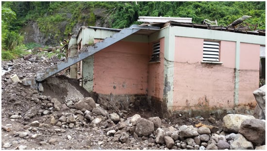
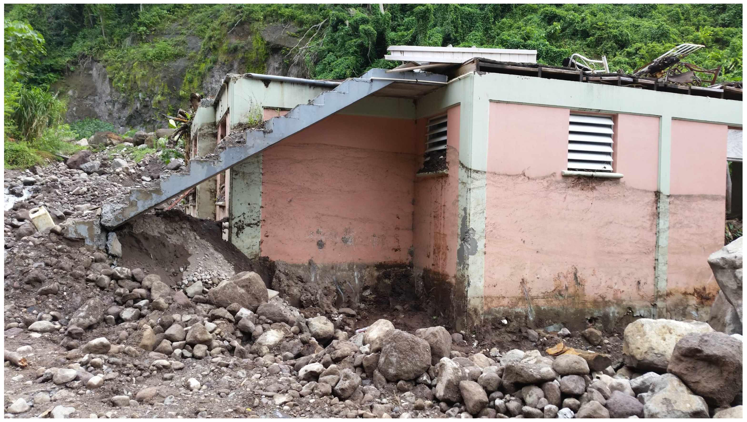
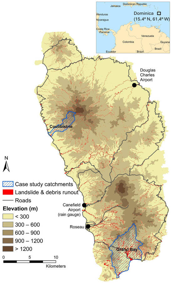
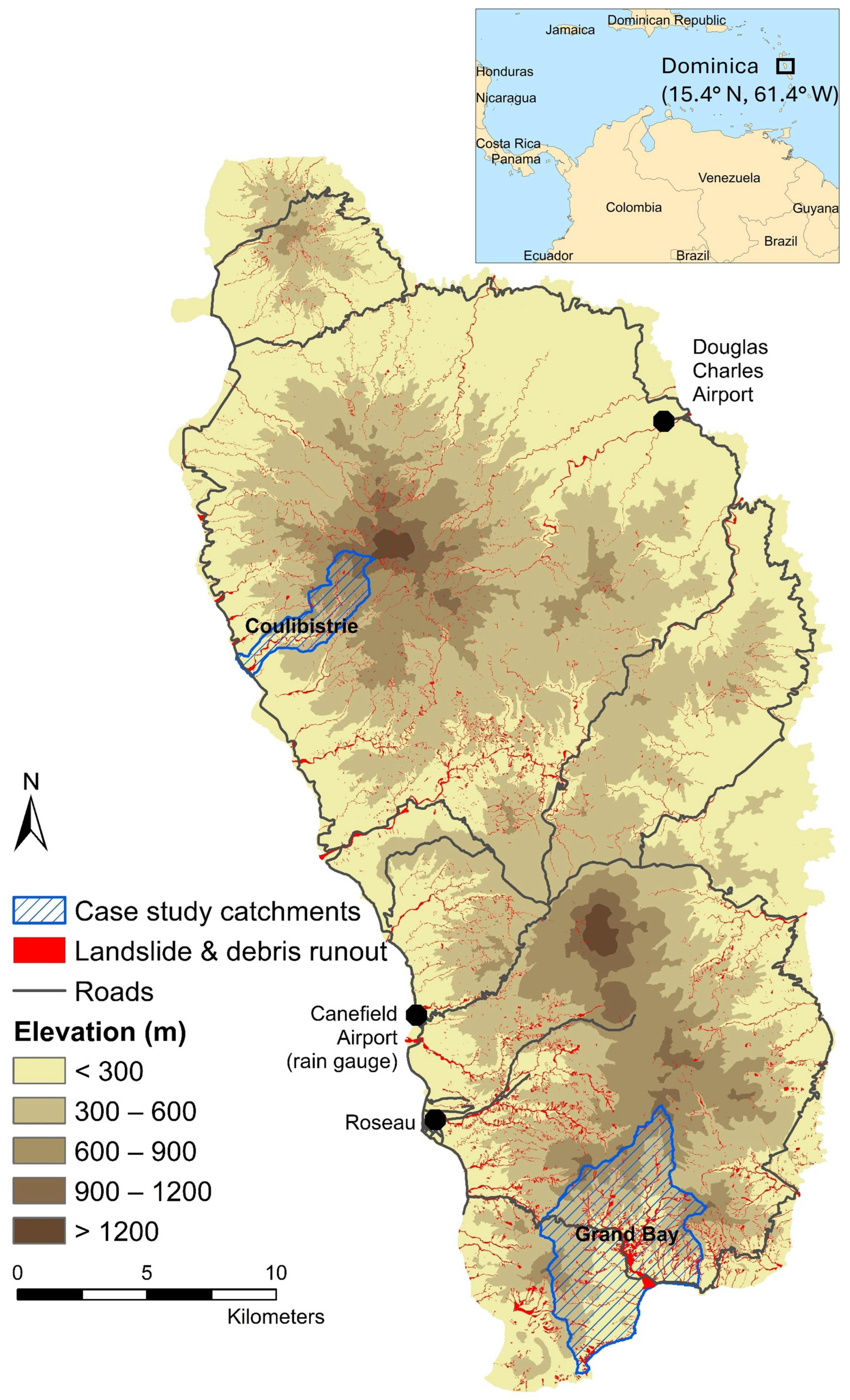
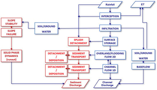
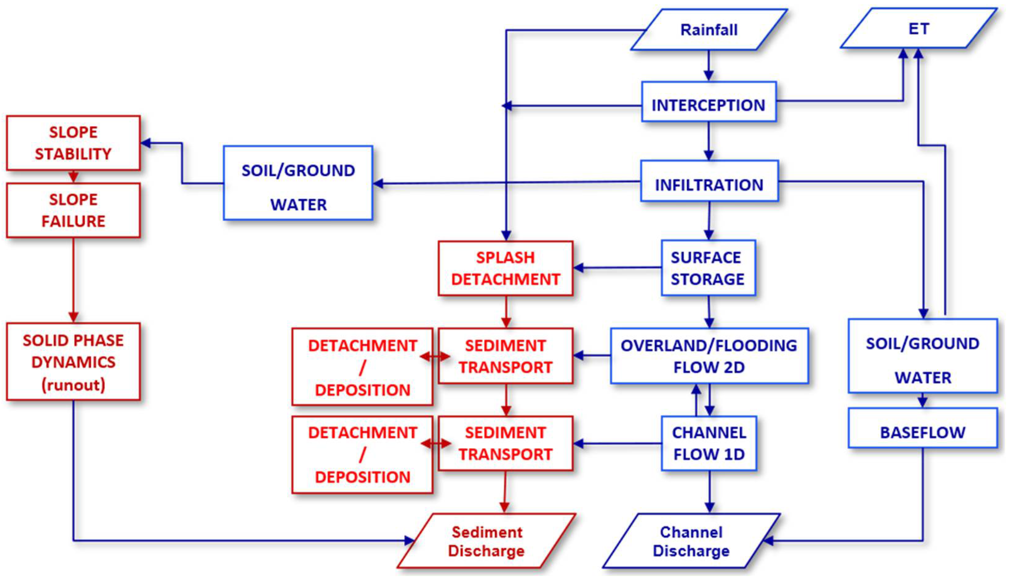
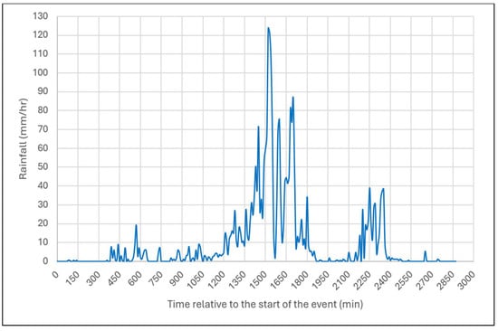
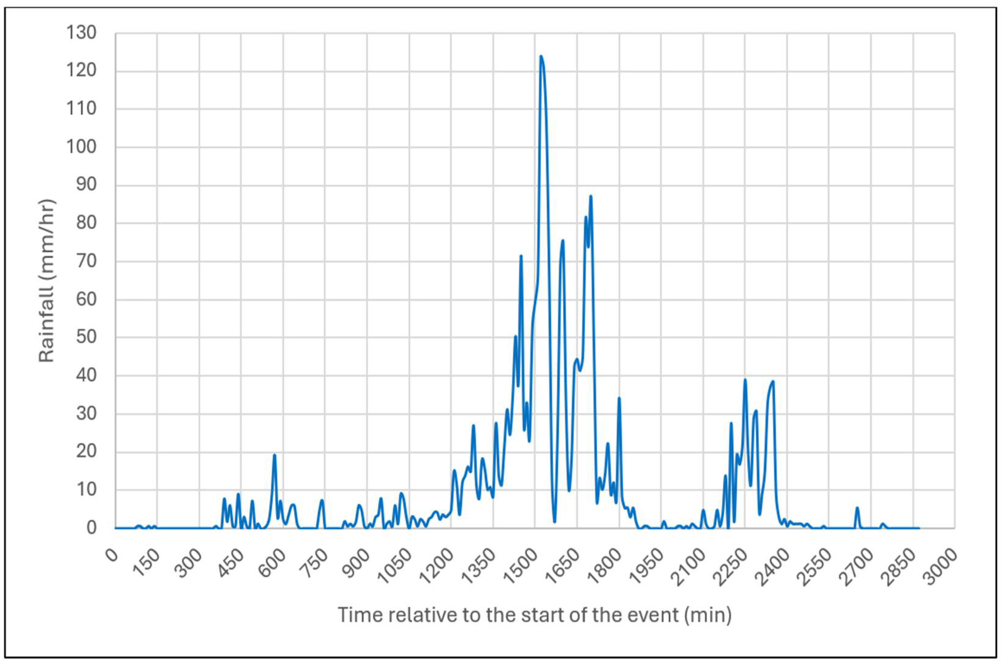
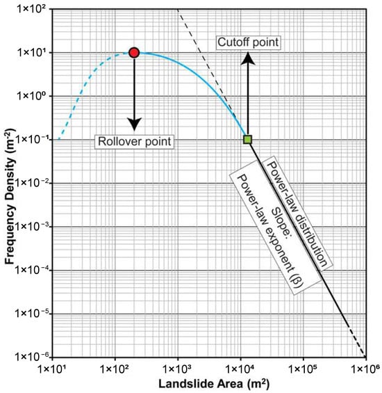
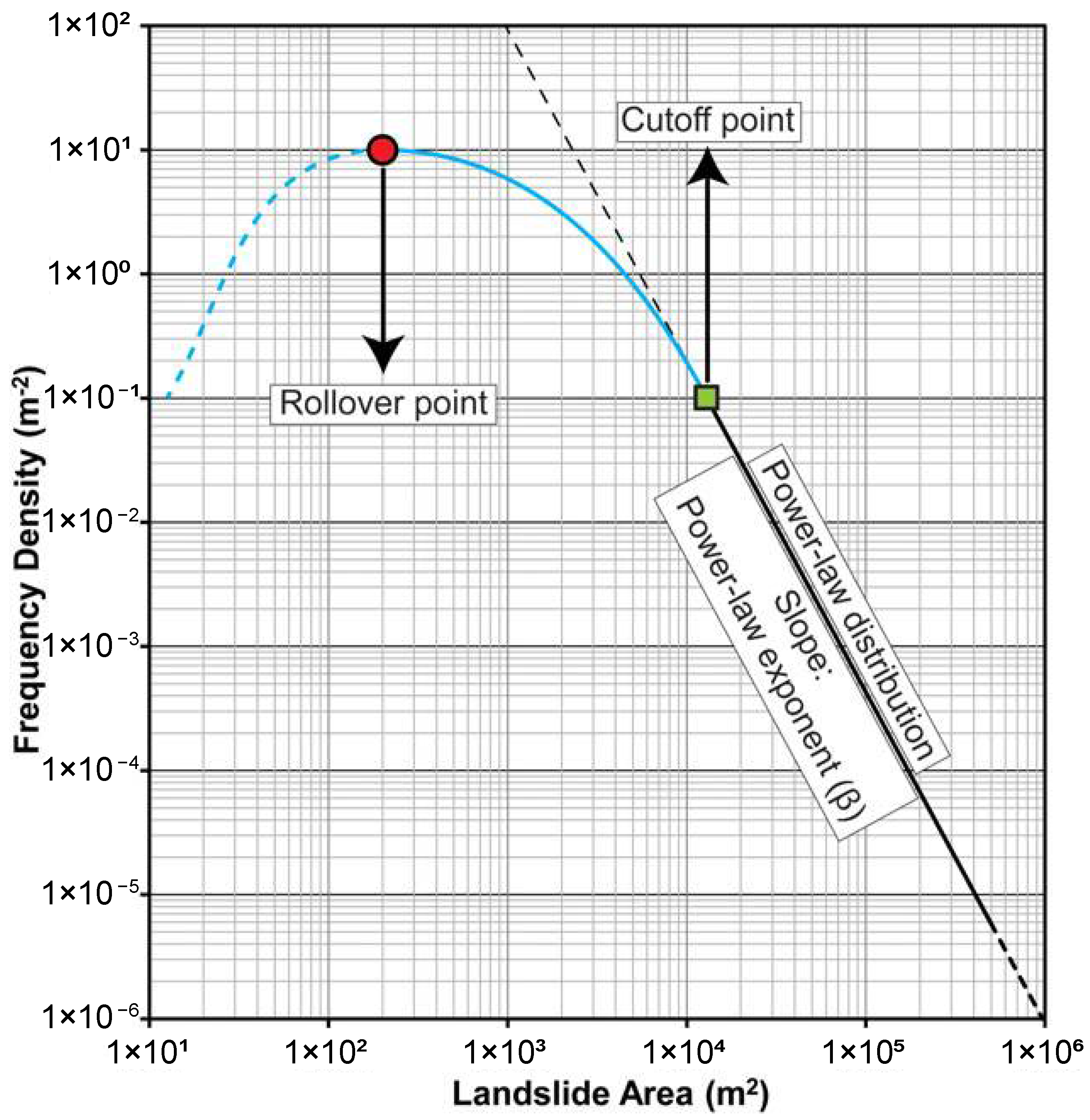
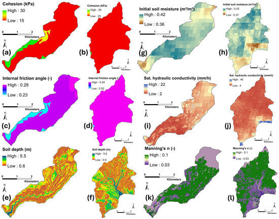
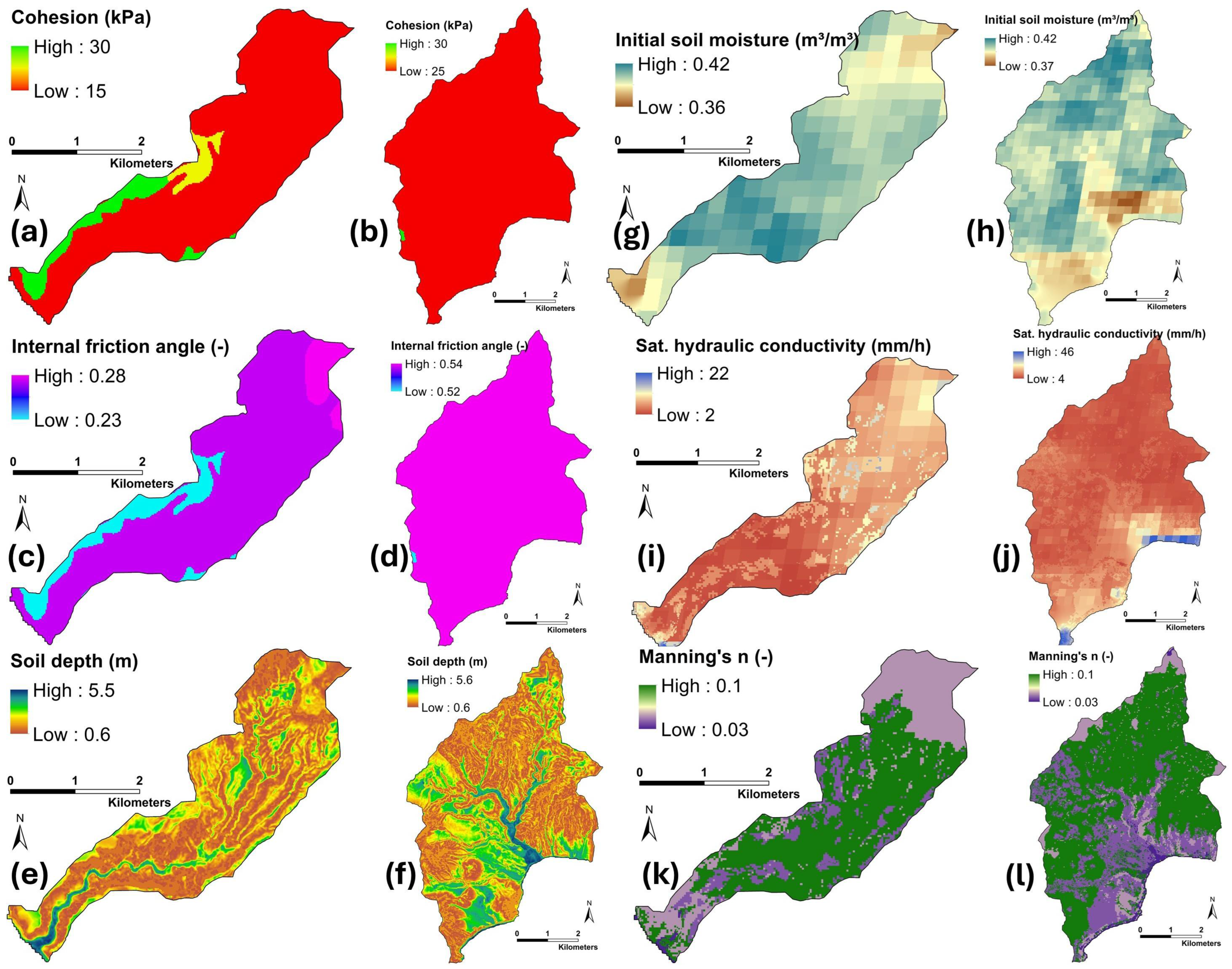
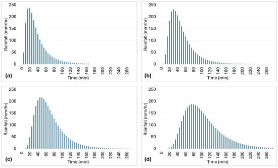
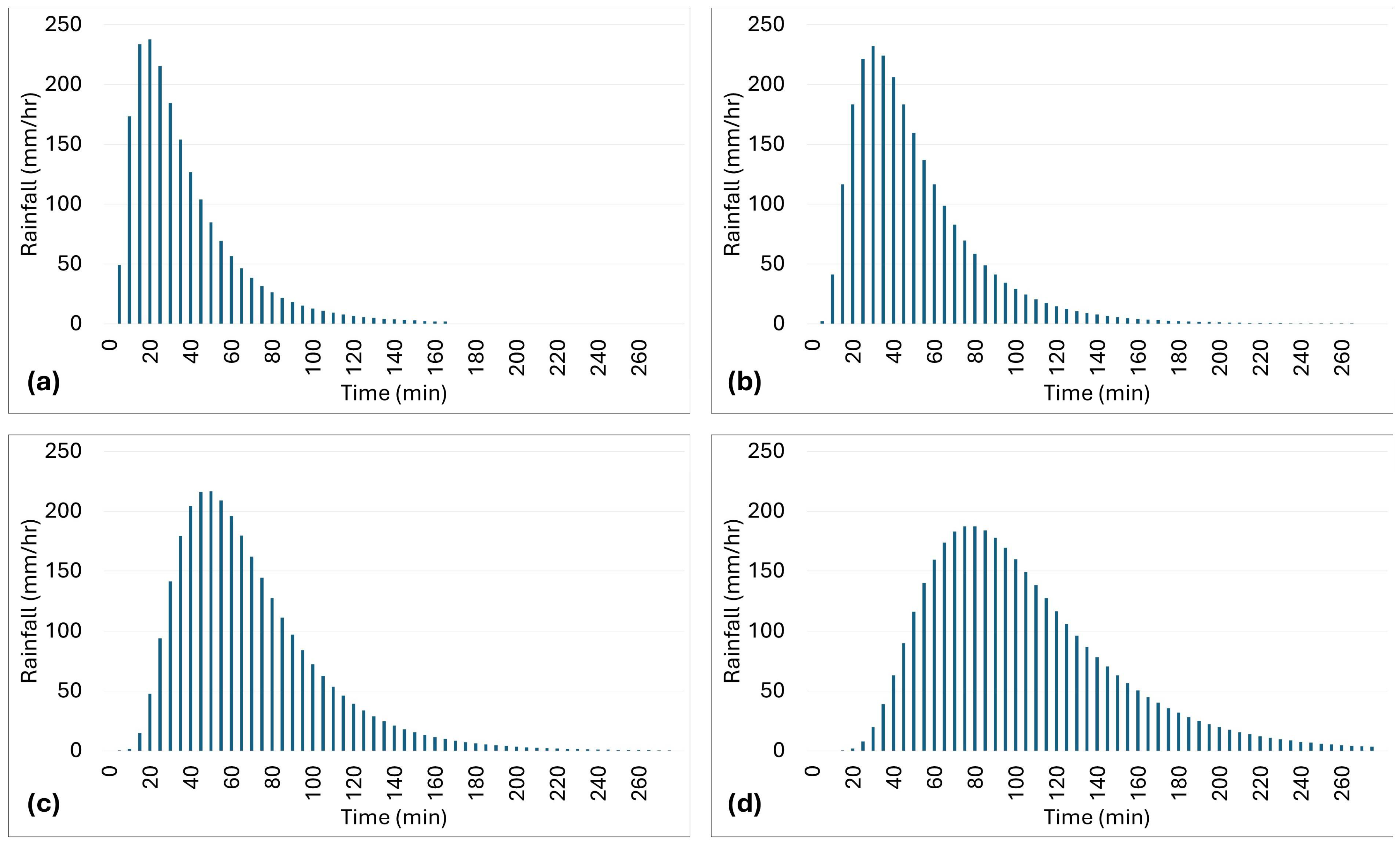
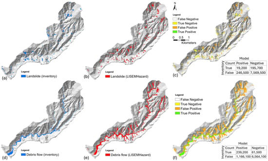
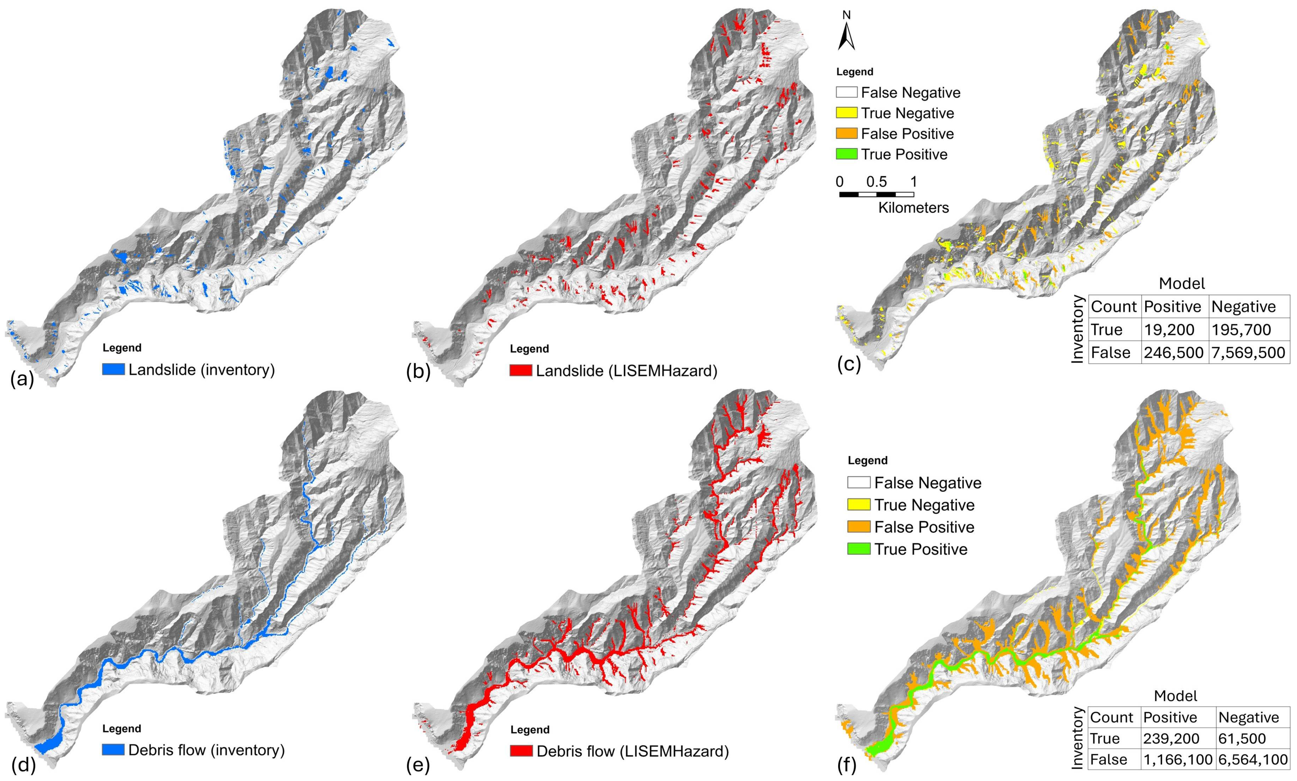
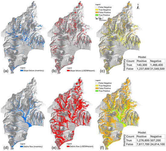
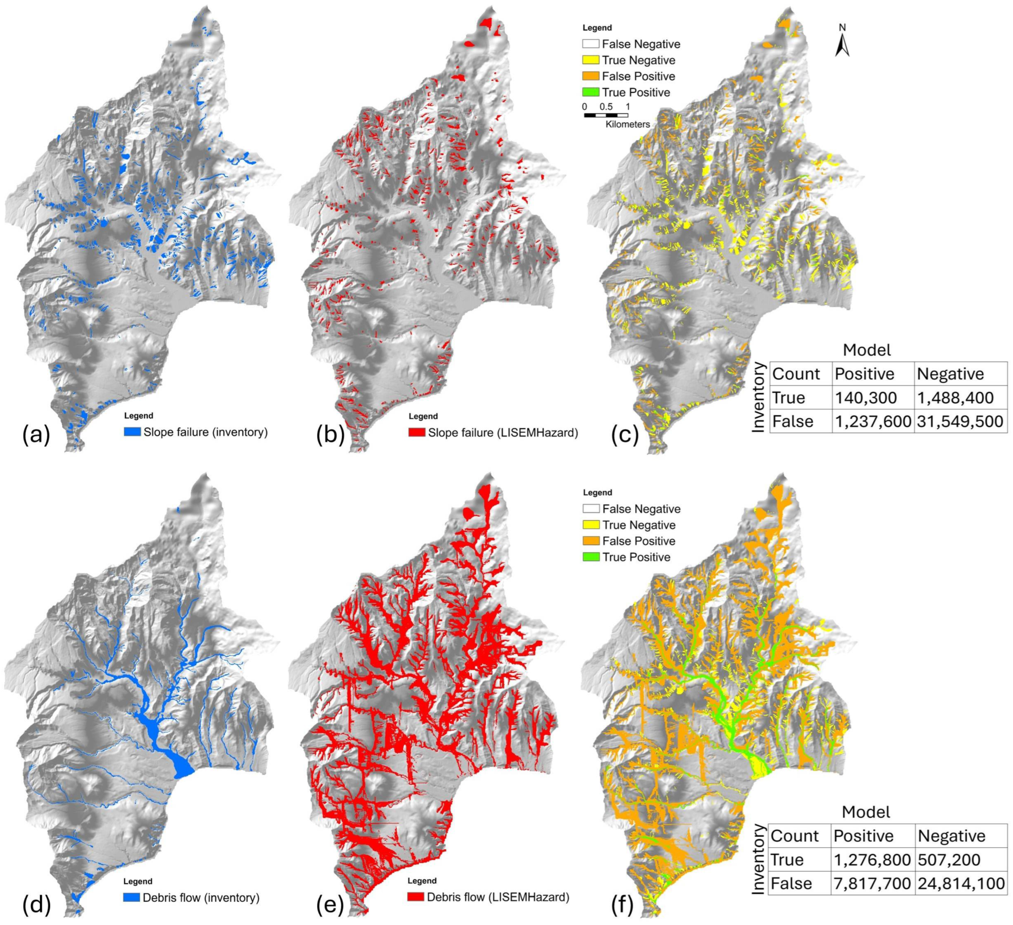
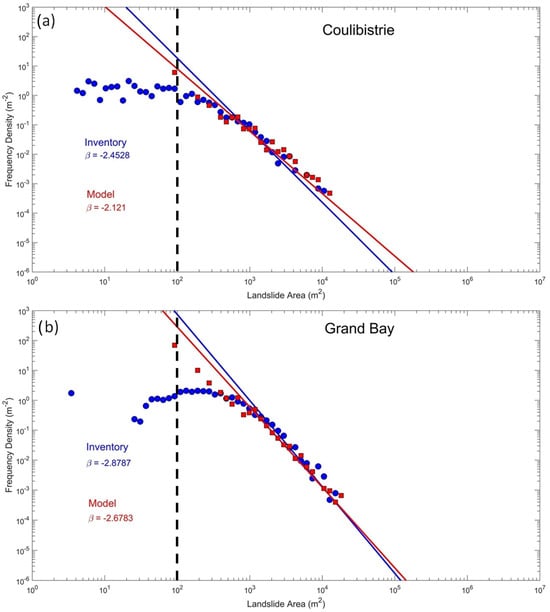
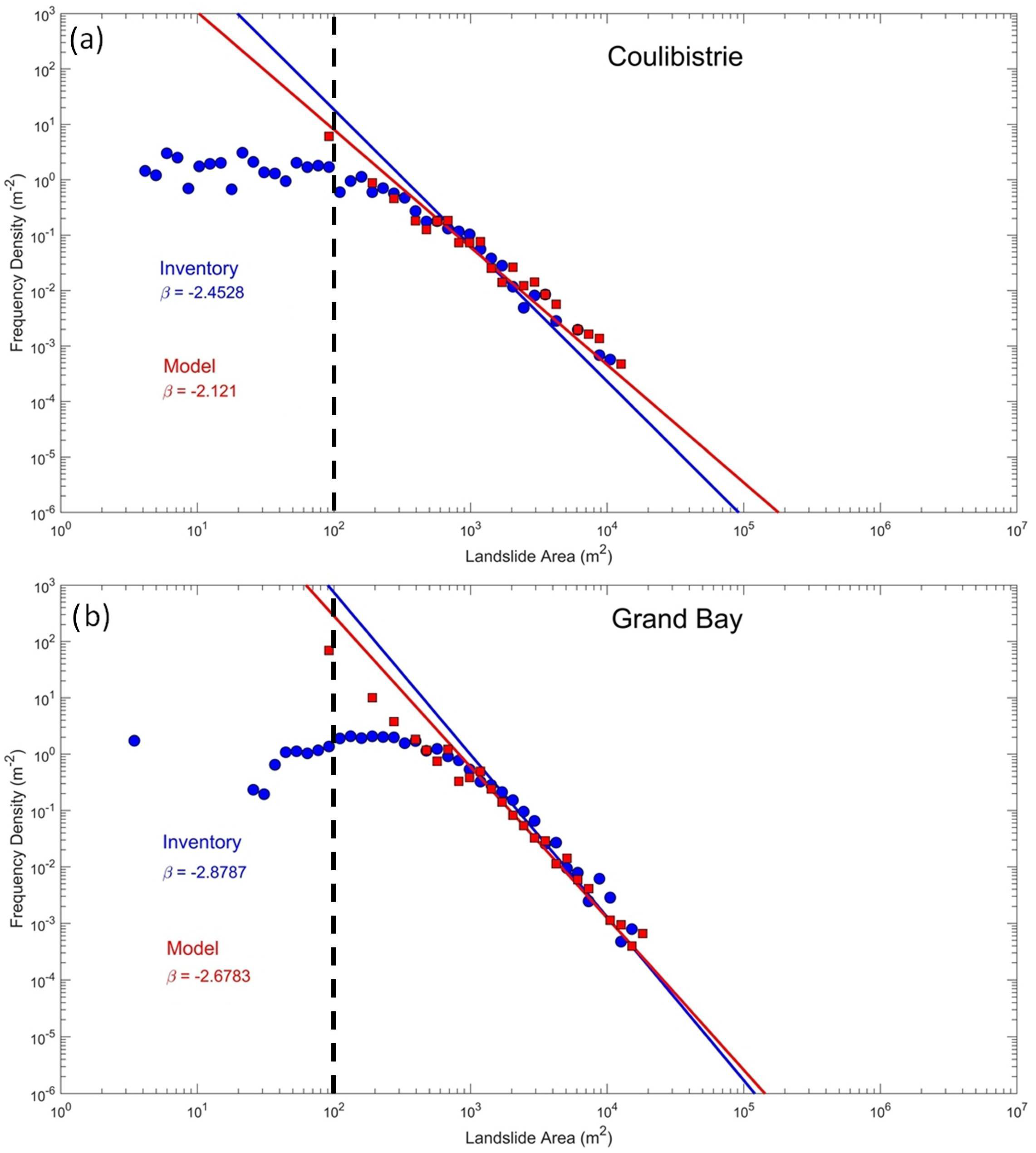
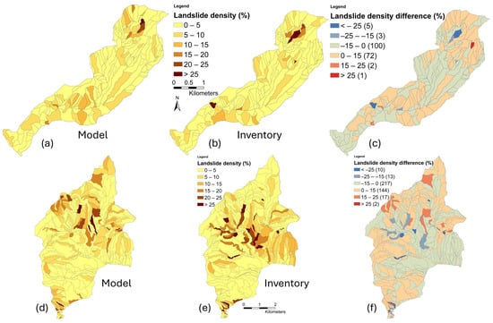
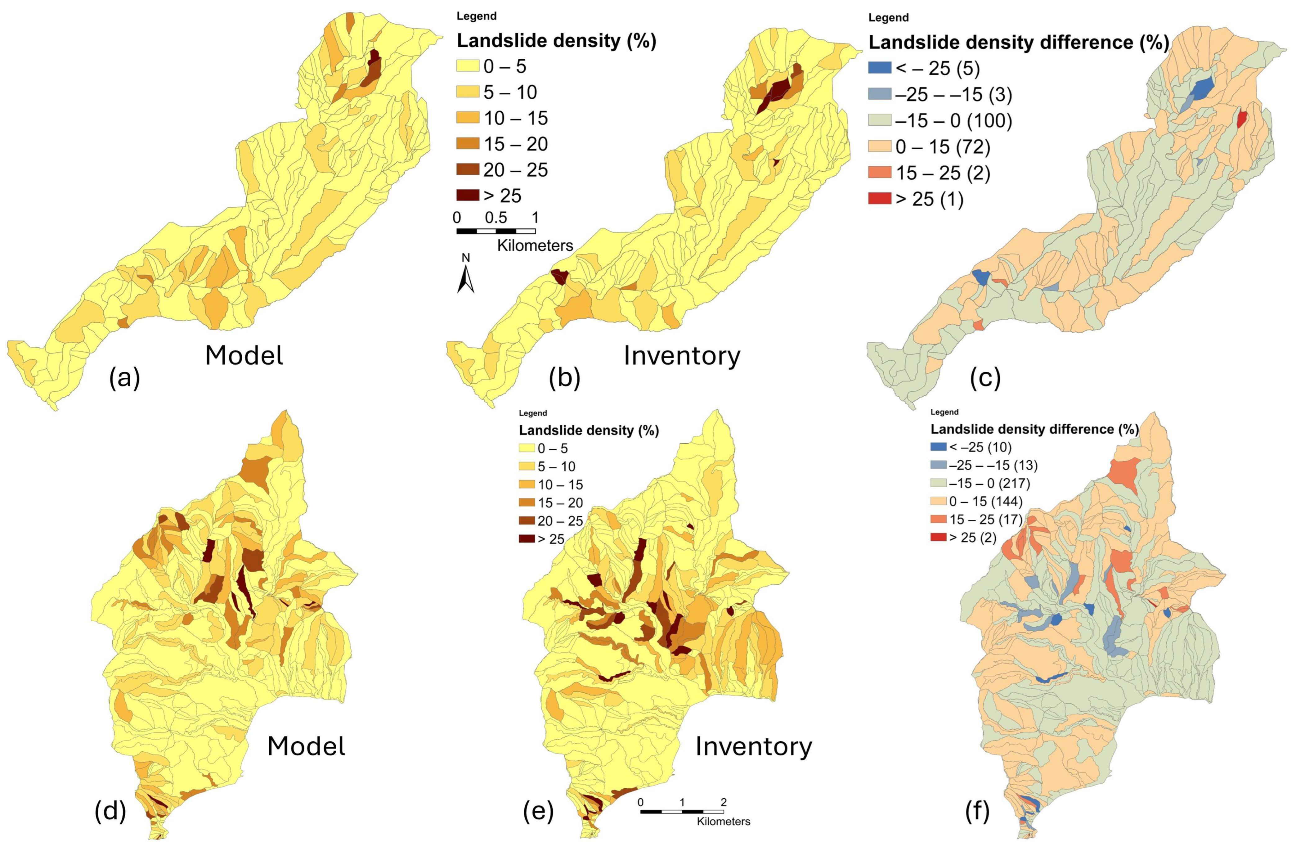
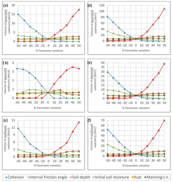
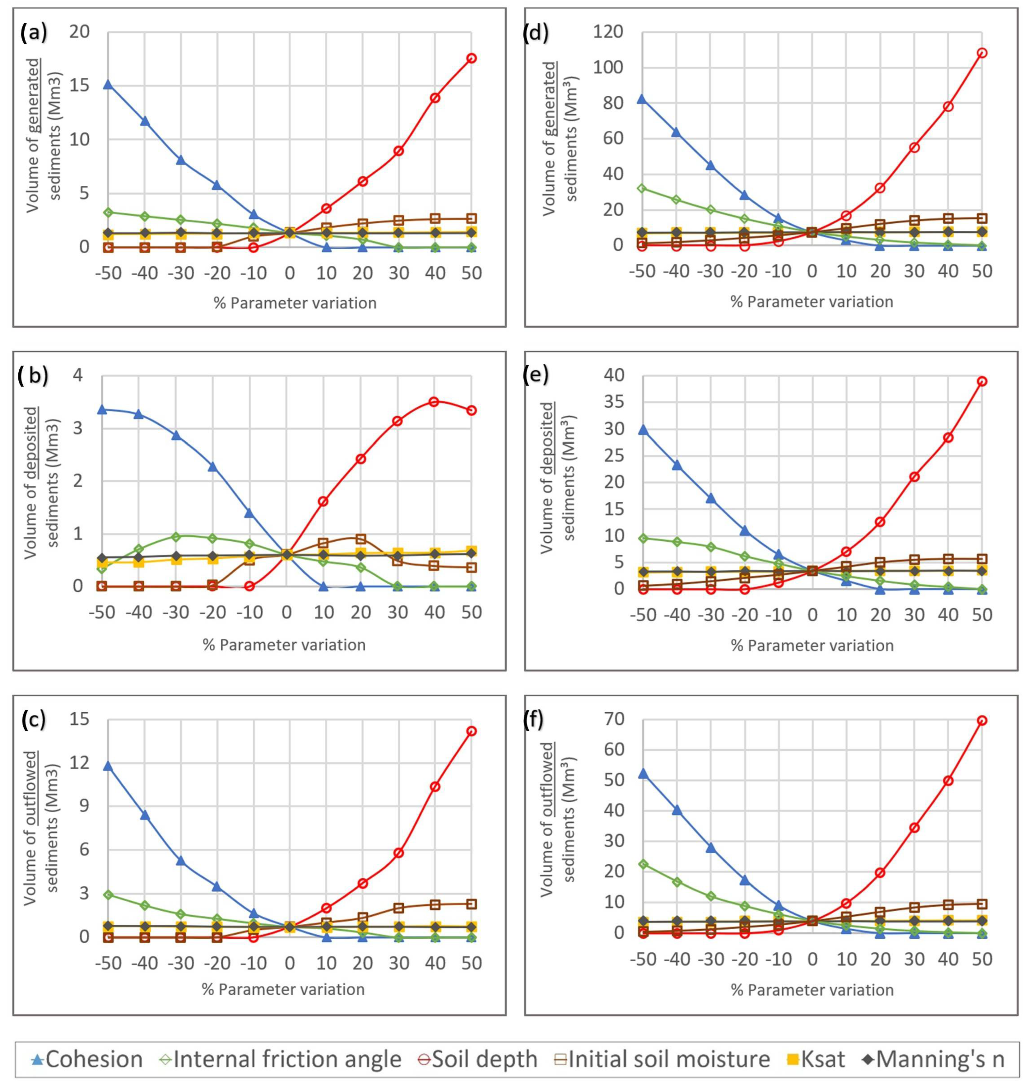
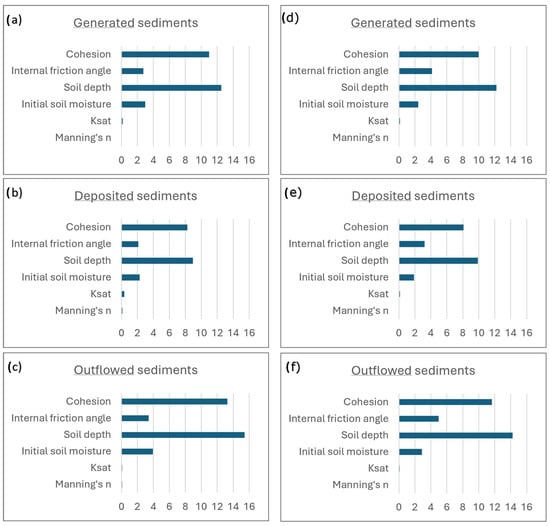
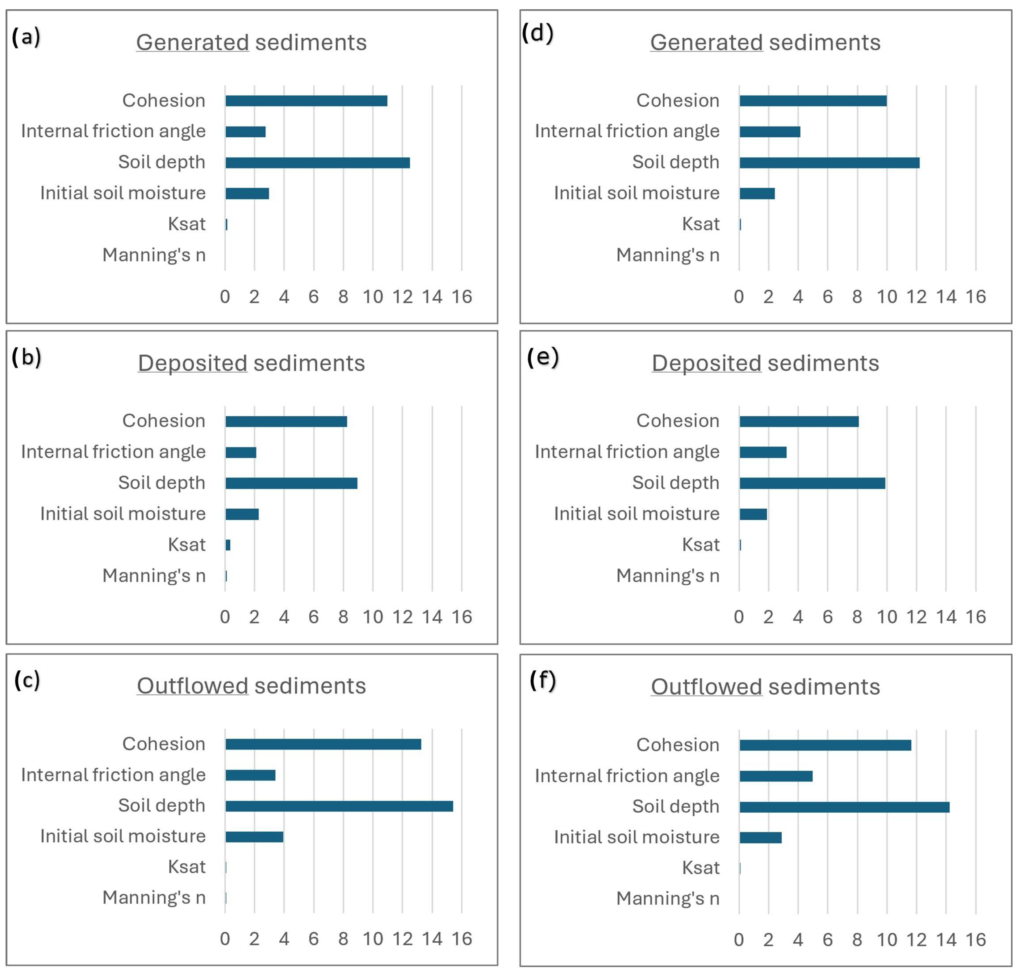
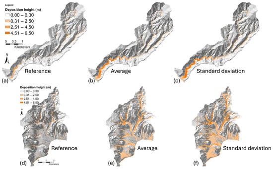
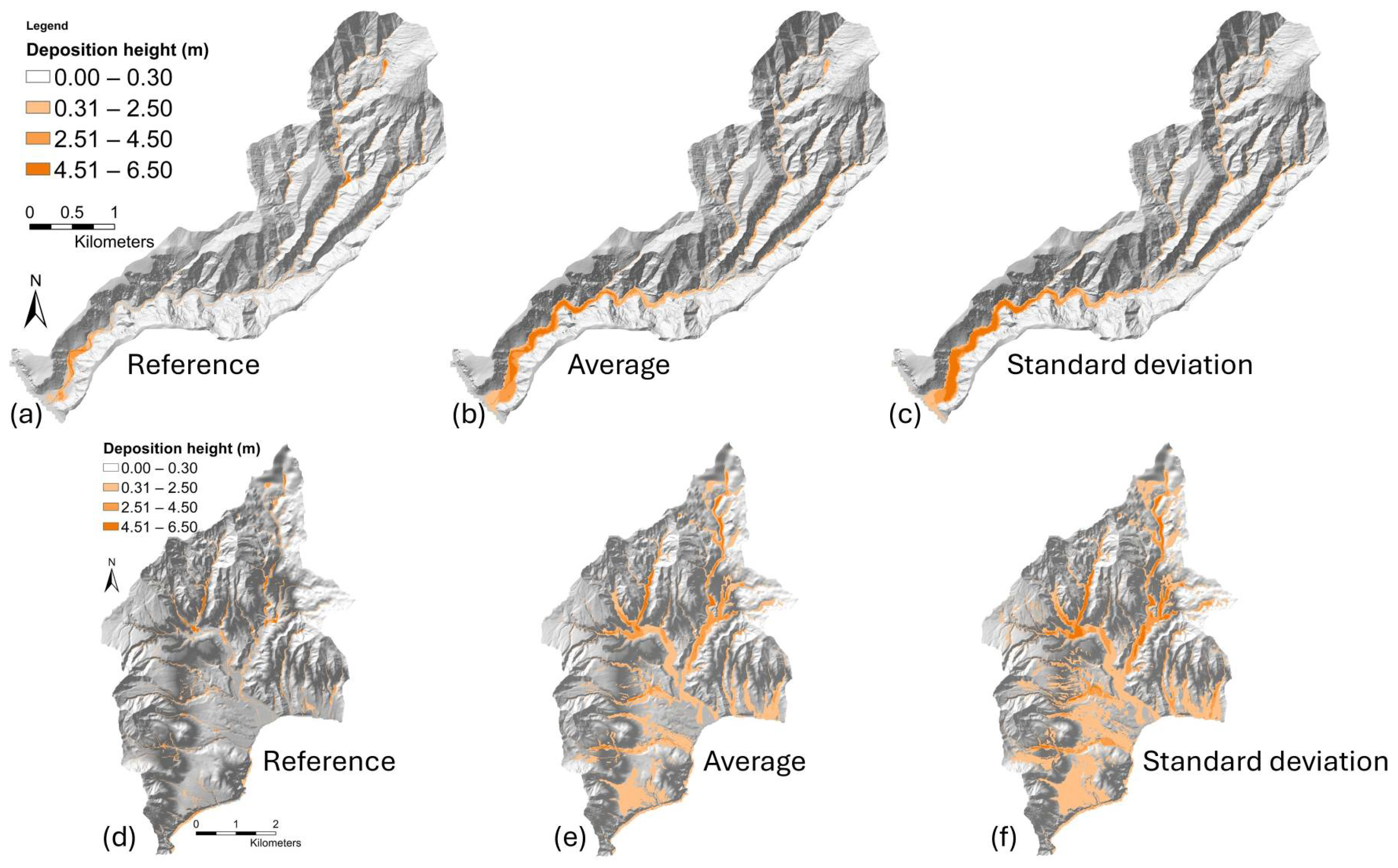
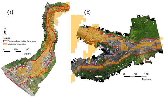
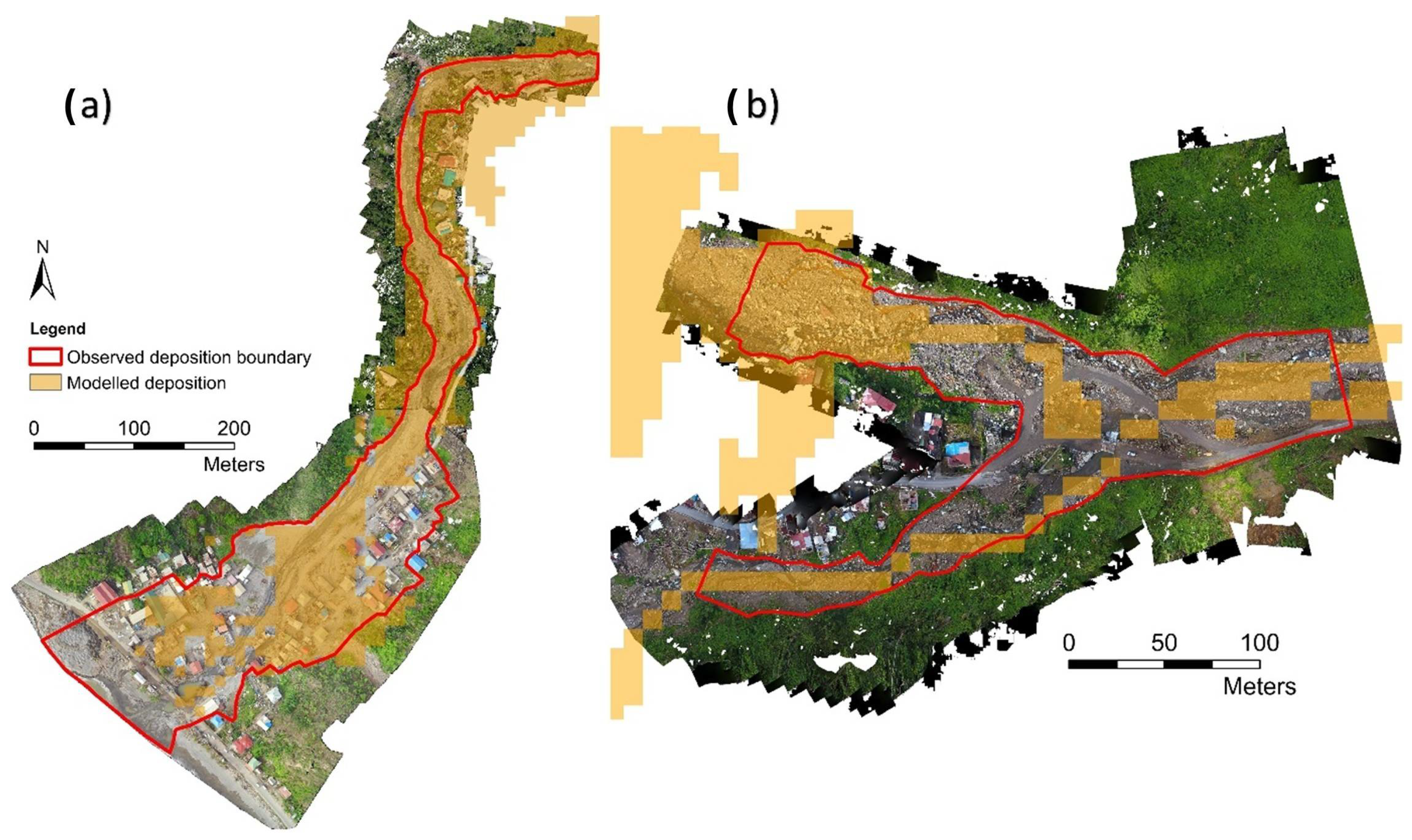
Disclaimer/Publisher’s Note: The statements, opinions and data contained in all publications are solely those of the individual author(s) and contributor(s) and not of MDPI and/or the editor(s). MDPI and/or the editor(s) disclaim responsibility for any injury to people or property resulting from any ideas, methods, instructions or products referred to in the content.

Article Metrics

Citations

Article Access Statistics

Journal Statistics

Multiple requests from the same IP address are counted as one view.

Model	Process Types								References
Model	Soil and Surface Hydrology	Surface Erosion	Slope Failure	Sediment Transport	Entrainment	Deposition	2D Flow/Flooding with Sediment	Flood/Debris Flow	References
Erosion 3D	✓	✓	-	✓	-	✓	-	-	Defersha, et al. [36]; Schmidt, et al. [37]; Schindewolf and Schmidt [38]
Hairsine-Rose	✓	✓	-	✓	✓	✓	-	-	Hairsine and Rose [39]; Hairsine, et al. [40]
SINMAP	-	-	✓	-	-	-	-	-	Dietrich, et al. [41]; Montgomery and Dietrich [42]; Pack, et al. [43]
SHALSTAB	-	-	✓	-	-	-	-	-	Dietrich, et al. [44]; Dietrich, et al. [41]; Montgomery and Dietrich [42], Dietrich, et al. [45]
Delft-3D-FLOW	✓	✓	-	✓	-	✓	✓	-	Deltares [46]; Fauzah, et al. [47]; Theol and Charlotte de Fraiture [48]
Sobek	-	-	-	✓	-	✓	-	-	Betrie, et al. [49]; Deltares [50]; Ji, et al. [51]
WEPP	✓	✓	-	-	-	✓	-	-	Flanagan, et al. [52]; Foster and Lane [53]
Eurosem	✓	✓	-	✓	-	✓	-	-	Morgan, et al. [54]; Morgan, et al. [55]
OpenLISEM	✓	✓	-	✓	-	✓	✓	-	Baartman, et al. [20]
KANAKO 2D	-	✓	✓	✓	-	✓	✓	✓	Nakatani, et al. [56]; Nakatani, et al. [57]
FLO-2D	-	-	-	✓	-	-	✓	✓	Calligaris, et al. [58]; Cesca and d’Agostino [59]; O’Brien, et al. [60]
Debris-2D	-	-	✓	✓	-	✓	✓	✓	Chae, et al. [61]; Liu and Huang [62]; Liu and Wu [63]; Wu, et al. [64]
Flow-R	-	-	✓	✓	-	-	-	-	Ali, et al. [65]; Chen, et al. [66]; Horton, et al. [67]
EDDA	-	-	✓	✓	✓	✓	✓	✓	Chen and Zhang [68]; Shen, et al. [69]
TRENT 2-D	-	✓	-	✓	-	✓	✓	✓	Armanini, et al. [70]; Rosatti and Begnudelli [71]
RAMMS	-	-	-	✓	✓	✓	✓	✓	Bartelt, et al. [72]; Cesca and d’Agostino [59]; Simoni, et al. [73]
LISEMHazard	✓	✓	✓	✓	✓	✓	✓	✓	Bout, et al. [74]; Van den Bout, et al. [75];

Data	Spatial Resolution	Time of Acquisition	Description	Source	Derived Variables
Precipitation	-	18 to 19 September 2017	Full record of the event with 10-min timestep	Weather station in Canefield airport of Dominica	Rainfall
DTM	0.5 m	19 February to 5 May 2018	LiDAR DTM with 0.05 m vertical accuracy	Dominica’s National Physical Planning Department [105]	Slope, gradient, local drain direction, channels network, accumulated flux, outlet location
Soil	250 m	1 January 1950 to 1 December 2015	SoilGrids product	Global gridded soil information [101]	Sand, clay, gravel, bulk density, plant available water content, porosity, initial soil moisture, saturated hydraulic conductivity, suction at wetting front, wilting point, field capacity, d50, d90, cohesion, aggregate stability, soil density, internal friction angle
Land use	5 m	1 January 1999 to 1 June 2015	SPOT 5 image classification	CHARIM Project (charim.net) [100]	Manning’s n, random roughness, canopy height, vegetation cover, leaf area index, compaction

		Predicted
		Positive	Negative
Actual	True	True Positive (TP)	True Negative (TN)
Actual	False	False Positive (FP)	False Negative (FN)

Parameter	Coulibistrie					Grand Bay
Parameter	Cohens Kappa	Accuracy	Sensitivity	Specificity	RMSE	Cohens Kappa	Accuracy	Sensitivity	Specificity	RMSE
landslides (modeled vs. observed)	0.355	0.945	0.003	0.443	-	0.306	0.921	0.004	0.546	-
Debris flows (modeled vs. observed)	0.481	0.847	0.035	0.050	-	0.436	0.758	0.049	0.061	-
Deposition height (modeled vs. field measurements)	-	-	-	-	0.75	-	-	-	-	1.87
Deposition height (modeled vs. DoD at field measurements locations)	-	-	-	-	0.72	-	-	-	-	-
Deposition height (modeled vs. DoD at 100 random locations)	-	-	-	-	2.09	-	-	-	-	2.24

Criteria	Coulibistrie			Grand Bay
Criteria	Model	Modeled Landslides with Empirical Volume Estimation	Inventory	Model	Modeled Landslides with Empirical Volume Estimation	Inventory
Density (number of landslides/km²)	24.66	-	57.28	14.75	-	44.03
Total surface area (10⁴ m²)	26.80	-	25.09	139.01	-	163.52
Total volume (10⁶ m³)	1.33	0.75	0.56	7.42	5.38	4.07