


Abstract
This study utilizes Digital Elevation Models (DEMs) with different spatial resolutions (SRTM 90 m, ASTER DEM 30 m, and ALOS PALSAR 12.5 m), Landsat-8 satellite imagery, and the Bouguer WGM-12 gravity model to analyze morphotectonic features in the Upper Guajira region of Colombia, a desert area in northern South America, area that is composed by low-relief serranías of Cabo de la Vela, Carpintero, Cosinas, Simarua, Jarara, and Macuira. Three DEMs were used to extract and map morphotectonic lineaments, drainage networks, and morphological features. Lineaments were characterised by azimuth frequency, length, density, lithological distributions, and geological timeframes, with support from a digitized geological map from the Colombian Geological Service (SGC). The analysis of the east–west (E-W) Cuisa fault, using the Riedel shear model, suggests a transtensional/transpressional tectonic regime influenced by the Caribbean and South American plates, characterised by NE-SW and E-W fault orientations. Lineaments were grouped into five geochronological categories based on the geological map, revealing a shift from NE-SW to E-W orientations from the Cretaceous period onward, reflecting the ongoing movement of the Caribbean plate. Folds and faults from this tectonic activity were enhanced using Landsat-8 band combinations. The WGM-12 model was separated into regional and residual signals, with the latter highlighting the serranías subregions. Residual gravity analysis revealed significant negative anomalies, suggesting lower-density lithologies surrounded by higher-density blocks. This pattern aligns with the regional geological framework and may reflect a crustal root or terrain dragging linked to the tectonic processes that shaped the serranías. Derivative residual gravity data also revealed lineaments oriented NE–SW, whose distribution extends beyond the morphometric boundaries of the subregions. The study found a strong correlation between structural and drainage patterns, demonstrating structural control over geomorphology. This study establishes a solid morphotectonic and geophysical framework for the Upper Guajira region, demonstrating how multi-resolution DEM analysis combined with gravity data can resolve regional deformation patterns, crustal architecture, and tectonic development along the Caribbean–South American plate boundary.
1. Introduction
Northern South America records a prolonged and dynamic history of orogeny and sedimentary basin development from the Late Cretaceous through the Cenozoic, driven by the complex interactions among the Caribbean, Nazca, and South American plates [1,2,3,4]. The southwestern margin of the Caribbean Plate forms a broad deformation zone approximately 600 km wide, located at the northernmost extent of the Andean orogen [5,6,7,8,9,10,11,12]. This region’s tectonic evolution reflects the intricate amalgamation of terranes bounded by the ongoing major strike-slip and thrust fault systems [13,14,15]. Oblique convergent margins like this one are commonly characterized by substantial lateral displacement of crustal blocks, which disrupts the continuity of orogenic belts and produces fragmented systems. This region (Figure 1) thus represents a geologically complex area [14,15,16,17].
Within this tectonic framework, the Upper Guajira region (Figure 1) represents a geologically intricate region situated at the northernmost tip of South America, on the Guajira Peninsula. Its geological structure has been shaped by multiple phases of deformation since the Proterozoic and is intimately linked to the tectonic interactions between the Caribbean arc system and the South American continental margin [9,17,18,19,20,21,22,23,24]. The most prominent tectonic structure in the study zone is the Cuisa Fault (CF)—a steeply dipping W-E-trending, right-lateral strike-slip fault exhibits an estimated lateral displacement of ∼15 km [25,26], associated with a Late Cretaceous–Paleogene convergence event that significantly offers new insights into the morphotectonic evolution of the Upper Guajira region through the analysis of satellite datasets, contributing to a refined understanding of its complex tectonic development.
Morphotectonic analysis involves the identification and interpretation of fault and fold systems, fracture patterns, and geological lineaments [27,28,29]. Geological lineaments, defined as linear or curvilinear features visible at the terrain surface, often correspond to faults, slope-breaks, or structurally weakened zones [30]. Mapping these lineaments is a widely used method for assessing neotectonic activity and subsurface structures [28,31,32,33]. Remote sensing techniques significantly enhance the analysis of extensive areas that would be challenging to examine using only field-based methods [33,34,35,36,37]. Numerous studies have highlighted the application of these methods in analyzing tectonics—particularly neotectonics—and their impact on the geomorphological evolution of landscapes [38,39,40]. It is important to note that lineaments refer to linear geomorphic or structural elements identified from remote sensing data, and morphotectonic features to landforms directly related to tectonic activity.
Drainage network analysis complements lineament mapping by capturing tectonic deformation in the orientation and geometry of river channels. It supports the identification of faults, fractures, and geomorphological anomalies linked to recent and sub-recent tectonic activity [30,31,33,39,41,42,43]. Bedrock deformations caused by uplift, subsidence, or extensional and compressional forces can produce detectable changes in fluvial systems [33,40]. Drainage patterns, in both elevation and horizontal geometry, reflect the interaction between surface processes and structural propagation, providing valuable insight into regional tectonic configuration [33,39,42]. Considering the tectonic and lithological control on drainage patterns and their geomorphic response, their analysis is a useful tool for reconstructing tectonic histories. In this study, morphometric techniques based on satellite imagery are applied to improve the understanding of structural and neotectonic evolution.
Figure 1.
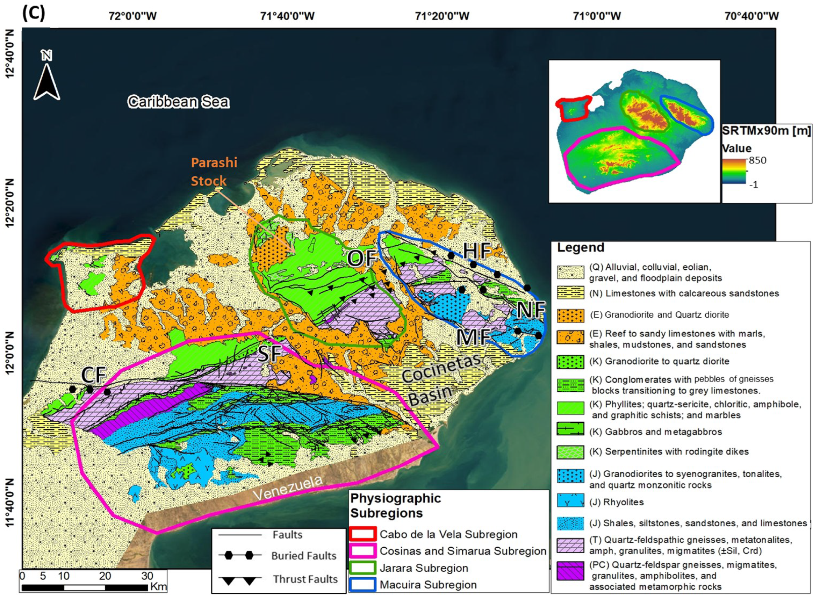
Regional tectonic setting between the Caribbean and South American plates and main tectonic features of the Upper Guajira region. (A) Tectonic frame of South America. NAB: North Andean Block, Car: Caribbean Plate, Nzc: Nazca Plate, Coc: Cocos Plate, Nam: North American Plate, Afr: African Plate, GS: Guyana Craton, Ec-Col-Ve: Boundaries between Ecuador, Colombia and Venezuela. Huancabamba Deflection zone is represented in a black dashed line (after Cediel et al., 2002 [10]). (B) Current tectonic map of the Caribbean area with movement rates of the different tectonic plates (modified from Weber et al., 2011 [44] & Quintero-Ortiz, 2017 [23]), with the Colombian Geological map from Gómez et al. (2015) [45]. CC: Central Cordillera, CHC: Choco block, CHR: Chortis block, CHT: Chorotega block, CF: Cuisa Fault, EC: Eastern Cordillera, EPF: El Pilar Fault, HEFZ: Hess Escarpment Fault Zone, MAY: Maya block, NPDB: North Panama Deformed Belt, PR: Perijá Range, OF: Oca Fault, SCDB: South Caribbean Deformed Belt, SMBF: Bucaramanga-Santa Marta Fault system, SNSM: Sierra Nevada of Santa Marta, WC: Western Cordillera. (B1) represents the red box the Guajira Peninsula and a NE-SW regional seismic cross-section interpretation from the National Hydrocarbons Agency (ANH) [46]. (C) Generalized geologic map of the Upper guajira after Gómez et al. (2015) [45]. HF: Huimatirra Fault, MF: Macuira Fault, NF: Nazareth Fault, OF: Osorio Fault, SF: Simarua Fault. Units were divided by their chronological period.
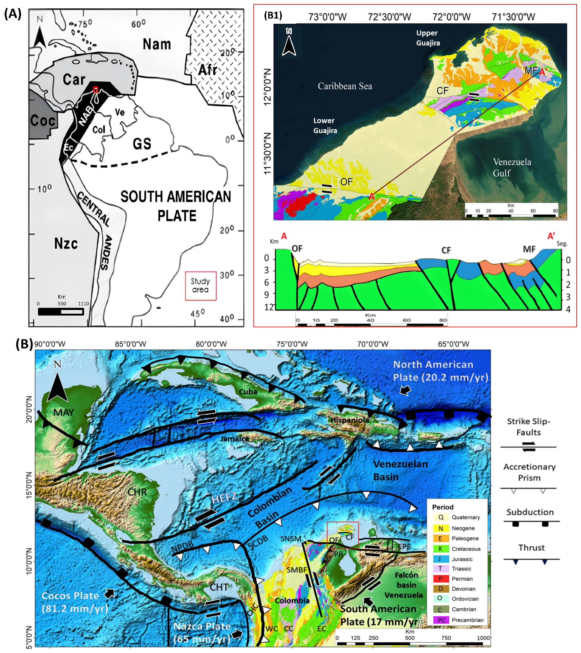
Satellite imagery and topographic data are widely used for the identification, extraction, interpretation, and mapping of morphotectonic lineaments and drainage networks [28,31,33,37,47,48,49,50,51,52]. Advances in Geographic Information Systems (GIS) have significantly improved the detection, visualization, and analysis of such features. In this study, satellite imagery, digital elevation models (DEM) of varying spatial resolution, and regional gravity data are integrated to investigate the morphotectonic framework of the Upper Guajira region. No similar analysis has been reported in this zone.
This study examines the morphotectonic characteristics of the arid Upper Guajira region in northern South America, a crucial segment along the Caribbean–South American plate boundary where deformation commenced in the Late Cretaceous and has persisted to the present day. The area was selected because of its isolation, limited vegetation cover, and the availability of high-resolution satellite datasets, which create an exceptional natural laboratory for identifying lineaments and tectonic landforms. The objectives of this work are to: (1) employ satellite datasets (DEMs, Landsat-8 imagery, and the WGM-12 gravity model) to examine lineaments, drainage networks, and morphostructural features; (2) interpret the structural framework and tectonic evolution of the region in the context of transpressional deformation; and (3) establish a methodological workflow for performing tectonic and geomorphological analyses in remote, arid, and structurally complex environments. This methodology can be applied to other regions worldwide that exhibit comparable plate interactions and arid conditions, thereby supporting comparative investigations of morphotectonic evolution across diverse geological settings.
2. Geologic and Tectonic Setting
The Northern Andean Block (NAB) (Figure 1A) is a microplate located in the northwestern corner of South America, extending from the Huancabamba deflection in north-central Peru to the Caribbean region. It encompasses the Cordilleran belts of Ecuador, Colombia, and Venezuela [11]. The NAB is composed of a tectonic mosaic of parautochthonous and allochthonous fragments with continental, pericratonic, and oceanic affinities, assembled through long-lived interactions among the South American, Caribbean, Nazca, and Farallon plates. Its Caribbean margin has undergone transtensional to transpressional deformation, which promoted the accretion of oceanic terranes onto the South American plate [13,14,22,53,54,55,56,57]. The NAB was shaped by three main collisional orogenic events—the Grenville (mid-Proterozoic), Quetame (Ordovician–Silurian), and a Permo-Triassic orogeny—followed by a taphrogenic phase referred to as the Bolívar Aulacogen [13,58,59,60]. The subsequent Andean Orogeny, initiated in the Cretaceous, was driven by subduction of the Caribbean Plate, which likely originated from Galápagos hotspot–related large igneous activity. These events, collectively known as the Caribbean Large Igneous Province (CLIP), began migrating eastward around 90 Ma [4,61,62].
In northern Colombia, the NAB reaches its northernmost continental extent, where the continuous Andes physiography transitions into discontinuous uplifted massifs surrounded by thick Cenozoic basins extending toward the Caribbean Sea (Figure 1B) [55,63]. As the Caribbean Plate drifted eastward from the Pacific, the northwestern margin of South America developed into a broad zone of oblique convergence and right-lateral deformation, generating transtensional to transpressional tectonic events recorded in blocks such as the Sierra Nevada of Santa Marta (SNSM) and Upper Guajira, both structurally and lithologically linked to the Central Cordillera (CC) [3,63,64,65,66,67].
The Guajira Peninsula is bounded by two dextral strike-slip faults: the CF, separating the Upper and Lower Guajira basins, and the Oca Fault (OF), which delimits the peninsula to the south from the SNSM block [2,53]. The Upper Guajira consists of low-relief serranías (e.g., Cabo de la Vela, Carpintero, Simarua, Cosinas, Jarara, Macuira) bordered by plains [68,69,70] (Figure 1C). Palinspastic reconstructions suggest these serranías were part of a pre-Andean uplift connected to the southwestern SNSM and CC until the Cretaceous–Paleogene collision of the Caribbean Plate with the continental margin [2,3,55,70,71,72]. The Lower Guajira is a basin containing a significant depocenter of stacked sedimentary sucessions, with Quaternary and Neogene units currently exposed and Cretaceous rocks found at depth in the basement (Figure 1(B1)) [17,24,73].
The Upper Guajira ranges comprise three main lithostratigraphic belts: (1) a weakly deformed Mesozoic volcano-sedimentary sequence resembling units in the southeastern SNSM and Perijá Range (PR) [68]; (2) a metamorphic sequence of Grenvillian and Late Paleozoic to Triassic age [67,70,74,75], intruded by Late Jurassic plutons [74]; and (3) Upper Cretaceous greenschists interlayered with mafic-ultramafic plutonic rocks [70,75]. In Cabo de la Vela, isolated Cretaceous mafic and ultramafic remnants crop out [56,70]. During the Eocene, Caribbean–South American plate interaction caused strike-slip movement along the CF [76] and normal faulting of crustal blocks, uplifting the serranías and the formation of the Cocinetas pull-apart basin [16,72], consisting of a 25-m-thick layer of late Pliocene sediment [72].
The tectonic evolution of the Caribbean began with the breakup of Pangea during the Triassic to Jurassic, which separated the North and South American plates. During this time, the continental Chortis Block detached from southern Mexico and rotated counterclockwise as the proto-Caribbean Plate began migrating eastward around 134 Ma [15,77,78,79,80]. This post-collisional, amalgamated area progressively advanced toward the east, initiating the formation of oceanic crust behind the western margin of the proto-Caribbean Sea. Jurassic (?) to Early Cretaceous oceanic crust, formed in the Pacific region, constitutes the current basement of the Colombian and Venezuelan Basins (Figure 1B) [62]. Radiometric data from the Guajira Peninsula reveal Early and Late Cretaceous basement ages [73], with crustal structures marked by reverse and normal faults, flower structures, and tectonic wedges that formed hydrocarbon traps within the Guajira Basin (Figure 1(B1)) [17,46].
As this oceanic crust migrated eastward between the Early and Late Cretaceous (72–125 Ma), it consumed the proto-Caribbean seaway created during the initial rifting between the American plates [81]. During this phase, the Hess Escarpment fault zone (HEFZ) developed as a major left-lateral fracture system within the Caribbean Plate (Figure 1(B1)) [62,81,82]. During the Late Cretaceous (99–65 Ma), an eastward-dipping subduction zone developed along the western margin of the proto-Caribbean Sea, generating an intra-oceanic island arc system known as the Great Arc of the Caribbean (GAC), potentially extending along the entire margin of North and South America [3,10,11,16,55,81]. At the same time, the region experienced widespread magmatic activity associated with the CLIP [4,62,81]. By ∼72 Ma, volcanism had largely ceased, and extensive basalt flows partially covered the Colombian and Venezuelan basins [62]. Certain areas of the Colombian and Venezuelan basis were unaffected by CLIP-related events, leading to the preservation of Jurassic to Early Cretaceous oceanic crust structures. Today, these appear as ridges and trough systems, with syn-sedimentary successions deposited before the Late Campanian [17,62].
The Late Cretaceous to Paleogene tectonic evolution of the northwestern Andean Cordillera and the northern South American–Caribbean margin was driven by oblique convergence between the Caribbean Plate—originating from the southwestern Pacific—and the South American margin. This interaction caused widespread deformation and the development of Cenozoic basins across northern Colombia and Venezuela, including the SNSM and the Guajira Peninsula [15,17,58,68,83]. Continued subduction during this period led to the formation of a short-lived Paleocene–Eocene magmatic arc [63,83].
In the Middle Eocene (∼43–37 Ma), the GAC with the Bahamas platform caused a change in the migration direction of the Caribbean Plate from northeastward to eastward [84]. This shift contributed to the formation of the Cayman trough pull-apart basin [3,55,72,85,86]. The Parashi plutonism, occurring between 47 and 51 Ma in the Guajira region, is associated with magmatism related to an immature oblique subduction zone [71]. During this period, the OF accommodated dextral displacement of the Caribbean Plate. The OF, marking the boundary between the SNSM and the Lower Guajira Basin (Figure 1), extends approximately 650 km eastward into western Venezuela [19] and connects westward to the Santa Marta–Bucaramanga Fault (SMBF) offshore [87] (Figure 1B). Estimated displacements along the OF range from 15 to 100 km [17,87]. The OF underwent a transition from vertical to dextral movement in the Late Eocene to Early Oligocene, with activity persisting into the Miocene and Holocene [19,64,87].
In the Late Oligocene (∼25 Ma), convergence triggered thrusting of the South Caribbean Deformed Belt (SCDB) and southeast-directed strike-slip/subduction within the Colombian Basin [1,2,10,24,88]. This phase may also coincide with tectonic uplift in nearby areas like the Perijá range [18,89]. The CF also began accommodating eastward motion of the Caribbean Plate during this time [25,76]. The fault extends ∼80 km offshore and continues onshore with a minor east-southeast strike, reaching ∼50 km into the Gulf of Venezuela [57,90]. Estimated displacements vary from 1 km to ∼15 km [25,68,91]. Its main activity spans the Late Eocene to Early Oligocene, with reactivation during the Early Miocene and continued vertical offset through the Late Miocene–Early Pliocene [25].
Neogene tectonics were dominated by strike-slip faulting and Andean uplift [86]. The Guajira Peninsula experienced transtensional faulting and east-west motion, shaping the modern landscape [72,89,92]. During the Middle Miocene (∼13 Ma), subsidence increased in several basins (e.g., Falcón), while deformation persisted across the region. By the Pleistocene, the Caribbean–South America plate boundary had nearly reached its present-day geometry. Continued shearing produced a 1200 km escarpment across the central Caribbean Sea [16,24,62,82,88], while deformation remains active in the SCDB along the southern Colombian Basin (Figure 1B).
3. Materials and Methods
3.1. Acquisition and Preparation of Remote Sensing Data
Satellite imagery, topographic data, and gravity information were processed to extract and analyze morphotectonic lineaments and drainage patterns across multiple spatial scales. A multispectral Landsat-8 OLI/TIRS image was used in conjunction with three DEMs of varying spatial resolutions—SRTM (90 m), ASTER GDEM (30 m), and ALOS PALSAR (12.5 m)—to evaluate scale-dependent expressions of structural features. Data processing and analysis were carried out using ArcGIS, ENVI 5.3, and PCI Geomatica 2012, enabling terrain analysis, image enhancement, and semi-automatic lineament extraction [28,33,93,94,95]. In addition, the World Gravity Model 2012 (WGM-12) Bouguer anomaly dataset was incorporated to identify lateral density variations and major crustal discontinuities relevant to regional tectonic interpretation [52,96,97,98,99,100].
Three DEM datasets with different spatial resolutions were used to analyze lineament patterns across varying scales of structural expression. The highest-resolution dataset (12.5 m) was derived from the Advanced Land Observing Satellite Phased Array type L-band Synthetic Aperture Radar (ALOS PALSAR) mission (2006–2011), operated by the Japan Aerospace Exploration Agency (JAXA), which employed L-band synthetic aperture radar capable of penetrating vegetation and cloud cover, making it suitable for detailed structural mapping [101]. Medium-resolution data (30 m) were provided by the Advanced Spaceborne Thermal Emission and Reflection Radiometer Global Digital Elevation Model (ASTER GDEM), developed jointly by the Ministry of Economy, Trade and Industry of Japan (METI) and NASA [102]. For broader-scale analysis, lower-resolution (90 m) elevation data from the Shuttle Radar Topography Mission (SRTM) were used, based on C-band radar interferometry [103,104]. While newer global DEM products may exhibit differences at fine spatial scales, the DEM datasets chosen for this study were intentionally selected for a controlled, multi-resolution analysis of scale dependence and dataset integration, rather than data availability or benchmarking based on recency or performance.
Preprocessing of DEMs is crucial for removing artificial spikes and isolated pixels that can distort surface modeling [105,106]. Such artifacts may arise from feature-matching errors, resolution limitations, or localized data noise rather than from real geomorphic processes. Given the arid conditions and limited anthropogenic influence in the Upper Guajira region, these distortions are expected to be minimal. Nevertheless, the presence of spurious sinks was systematically assessed, and the “Fill” algorithm implemented in ArcGIS 10.8 was applied conservatively to the DEM datasets to remove non-physical depressions while preserving genuine topographic gradients and structural lineaments relevant to morphotectonic analysis [107].
Landsat-8 captures 11 spectral bands, which include optical and near-infrared bands from the Operational Land Imager (OLI) and thermal bands from the Thermal Infrared Sensor (TIRS) [108]. The spatial resolution varies depending on the wavelength: 30 m for bands 1–7 and 9, 15 m for the panchromatic band 8, and 100 m for thermal bands 10 and 11 [109]. To prepare Landsat-8 scenes for analysis, ENVI 5.3 software was used for preprocessing, correcting radiometric and atmospheric distortions via the FLAASH toolbox. Two Landsat-8 OLI/TIRS (L8) scenes, covering the entire study area (Path/Row: 7-52 and 8-52), were obtained from the USGS Earth Explorer portal.
The WGM-12 is a global gravity dataset integrating satellite, airborne, and terrestrial gravity measurements. It combines data from satellites such as the Challenging Minisatellite Payload (CHAMP), Gravity Recovery and Climate Experiment (GRACE), Gravity Field and Steady-State Ocean Circulation Explorer (GOCE), and gravity models such as EGM 2008, DTU 10, and Global Topography 30 arc-second (GTOPO30), along with in situ gravity observations [97]. These datasets were merged using an iterative least-squares approach, incorporating spherical harmonic coefficients up to degree 2190 and order 2159 [96,97]. The dataset is provided at a 2.5 arc-minute (∼4.6 km) spatial resolution, using the World Geodetic System 1984 (WGS 84) datum and assuming a crustal rock density of 2.67 g/cm3 [96,97]. The WGM-12 model was selected for this study due to its effectiveness in regional and local mapping morphological and tectonic structures [52,99,100]. The WGM-12 Bouguer anomaly model for Upper Guajira was obtained from the International Gravimetric Bureau (BGI) gravity database at no cost.
Table 1 presents details of the datasets used in this study. All datasets were projected using the WGS-84 Universal Transverse Mercator (UTM) coordinate system, specifically Zone 19N. Figure S1 shows the processed DEMs and Landsat-8 true colour imagery, and a scheme of the workflow used in this research.
Table 1.
Information on remote sensing and gravity data used in the study.
The Colombian Geological Service (SGC) provides freely available geological maps through its online portal (https://www.sgc.gov.co/, accessed on 1 January 2025). The geological map of Upper Guajira, used in this study, was created by Gómez et al. (2015) [45] at a 1:1,000,000 scale. Lithological, structural, and hydrological information from this map was extracted and compared with the results obtained from the automatic delineation of lineaments and drainage networks.
3.2. Geological Lineaments
3.2.1. Digital Processing for Delineation and Identification of Linear Features
To identify geological lineaments, we extracted linear features from the DEMs, Landsat-8 (bands 7 and 8), and WGM-12 datasets. Hillshade techniques, commonly used in tectonically active regions, enhance linear features with specific trends [28,30,33,37,49,50,52,94,110]. These techniques simulate lighting effects, highlighting features that are perpendicular to the light source for maximum contrast [33,52,94].
To extract lineaments with different orientations, eight hillshaded raster images were created for each DEM using the hillshade tool in ArcGIS 10.8 (Figure S2). The first shaded relief image was illuminated from the north (i.e., the solar azimuth was 0°), with a solar elevation of 45° (ArcGIS default); for the other seven relief images, an identical solar elevation was used along with seven other illumination directions, including: 45°, 90°, 135°, 180°, 225°, 270° and 315°. Azimuth illumination and tilt values tend to hide or highlight morphological features in a hillshaded image, depending on their orientation with respect to the simulated light source. The next step consisted of applying the MDOW (multi-directional oblique weighted) shaded relief method [33,37,52], in which two multi-illumination hillshaded images were created from combinations of the individual shaded relief images. These combination images highlight lineaments and relief features with a variety of directions, which would not be visible if only a single shaded image was used. The first four shaded relief images were superimposed and combined to produce one image with multi-illumination directions (0°, 45°, 90°, 135°—Combination 1), and the four remaining images (180°, 225°, 270° and 315°—Combination 2) were processed in the same way (Figure S2). To conduct a comparative and complementary analysis for detecting geological lineaments, we utilized bands 7 and 8 of the Landsat-8 data. These bands have proven valuable for lithological discrimination and the extraction of morphotectonic features [33,50,51].
The Multi-illumination hillshaded images and the bands 7 and 8 of Landsat-8 were uploaded to the PCI Geomatica 2012 software [111] and a LINE algorithm was applied in each dataset in order to extract linear features (i.e., lineaments). LINE module requires three stages: (1) detection of edges, (2) thresholding of the image and (3) extraction of curves. The result for each dataset is a vector layer of polylines. The operation of the algorithm requires a group of parameters for its execution: RADI (Filter Radius) = 24; GTHR (Edge Gradient Threshold) = 70; LTHR (Curve Length Threshold) = 30; FTHR (Line Fitting Threshold) = 7; ATHR (Angular Difference Threshold) = 7; and DTHR (Linking Distance Threshold) = 70. The choice and understanding of each parameter were based on previous works [28,33,94] and the software manual [111]. Each vector layer was upload in ArcGIS 10.8 in order to be processed and analysed.
For the WGM-12 dataset, a similar processing approach was applied. However, unlike DEMs and Landsat-8 data, which are primarily designed for surface morphometric analysis, the WGM-12 model provides enhanced insights into deeper and shallower subsurface structures through gravity potential variations. Consequently, its process and interpretation will be deepened in the following section.
3.2.2. Methodology Used for the Analysis of Digital Lineaments
Numerical values for lineament lengths and orientations were extracted using the COGO tool in ArcMap 10.8. Some lineaments were manually excluded due to overlaps with anthropogenic features, such as roads and buildings, or due to image artifacts like cloud cover in ASTER DEM and Landsat-8 imagery (Figure S1; Table 2). The final lineament sets for each DEM configuration are displayed in Figure 2B,C. Additionally, the lineaments for Landsat-8 Bands 7 and 8 are presented in Figure S1(E1,E2).
Table 2.
Statistical summary of the automatic lineament maps, with the number and length of the extracted lineament samples from different surface images used.
Figure 2.
DistributionsDensities of lineaments obtained from different DEM images. (A) ALOS PALSAR (radar-derived DEM × 12.5 m); (B) ASTER DEM (optical-derived DEM × 30 m); (C) SRTM DEM (radar-derived DEM × 90 m). Numbering: (1) Combination 1; (2) Combination 2; (3) general frequency density map of both DEM lineament combinations. All density maps were generated using a radius of 1 km. Areas with maximum density anomalies likely indicate higher deformation intensity. The legend below the maps shows digital lineament lengths, and the percentages in the pie charts represent the proportion of lineaments for each combination.
To assess the dominant structural trends, this analysis considered several parameters [28,40,110]: (1) the number of lineaments (N), (2) total lineament length, (3) morphotectonic density (, where A represents the area), and (4) Azimuth orientation based on 5° bins across a full 360° range. The analysis of azimuth orientation was conducted using rose diagrams, which were created with Microsoft Excel’s dynamic table functionality for each group.
Various density maps were generated to visualize spatial distribution, highlight fault zones, and identify structural discontinuities and topographic breaks [43,48,95,112]. DEM-derived lineaments were then merged and classified according to the age of the geological units they intersect, based on the SGC geological map (Figure 1C). This classification subdivided the dataset into six chronostratigraphic intervals from the Quaternary to the Precambrian and enabled analysis of azimuthal trends through geological time [33].
This segmentation aimed to evaluate whether lineament orientations remain consistent within geological units of the same age and to assess how the datasets reflect structural evolution. Assigning lineaments to the stratigraphic units they intersect allows changes in orientation patterns to be tracked and related to the tectonic history of the region. The reliability of these temporal correlations depends on the accuracy of the geological map used by [45].
Using fault polylines from the SGC map and the regional tectonic context, a Riedel shear model was applied to assess strike-slip kinematics along the CF. Lineaments were identified as R and P synthetic shears, R’ antithetic shears, and associated tensile or compressional structures, consistent with expected Riedel patterns in transpressional regimes [33,37].
3.3. Geophysical Analysis of the Bouguer WGM-12 Dataset
The complete Bouguer anomaly dataset (WGM-12; Figure 3(A1)) was processed to separate regional (Figure 3(A2)) and residual (Figure 3(A3)) components, distinguishing long-wavelength signals linked to deep structures from short-wavelength anomalies associated with shallower sources [36,52]. This decomposition was performed using the MAGMAP tool in Geosoft Oasis Montaj, applying Fourier transformation, wavelength filtering, and phase matching to enhance crustal density contrasts [37,52,98,100]. High- and low-pass filters further refined the gravity field, isolating short-wavelength anomalies attributed to upper crustal features. A radial power spectrum analysis (Figure S3) identified a critical wavenumber of 0.02 cycles/km, corresponding to an estimated source depth of ∼10 km. Wavenumbers below this threshold represent deep-seated regional anomalies, while higher values highlight shallower residual signals [36,52].
Figure 3.
Geophysical regional and residual wave-cut and derivative results. (A1) Complete Bouguer WGM-12 dataset; (A2) Bouguer regional map; (A3) Bouguer residual map. WGM-12 Bouguer residual derivatives with their respective lineaments (brown): (B1) Analytic Signal (AS); (B2) Total Derivative Ratio (TDR); (B3) Total Derivative Cross (TDX); (B4) Total Horizontal Derivative (HDTDR). Each derivative map is displayed over an MDOW-based hillshade background (Combination 1) for visual reference only, to aid interpretation of structural discontinuities.
Derivative techniques were applied to the residual Bouguer WGM-12 dataset (Figure 3(A3)) to delineate geological boundaries and lineaments [52,98,100,113]. The Analytic Signal (AS), Tilt Derivative Ratio (TDR), Horizontal Tilt Angle Derivative (TDX), and the Total Horizontal Derivative of the Tilt Derivative Ratio (HDTDR) methods were used to highlight structural features such as faults, fractures, and intrusions, which are crucial for understanding regional geodynamics [52,98,114].
AS, also known as the total gradient, enhances potential field data by producing bell-shaped anomalies over sources, facilitating the determination of their positions and depths with minimal assumptions [115]. AS is defined as:
where f represents the potential field and , , and are its first derivatives along the x, y, and z axes, respectively. AS peaks over geological sources, making it a reliable tool for edge delineation [100] (Figure 3(B1)). Unlike TDR-based derivatives, AS remains unaffected by source inclination [115].
TDR enhances potential field features and detects the edges of causal bodies [116]. It is calculated as follows:
TDR values range between and radians (or −90° to 90°) regardless of the amplitude of the vertical derivative or total horizontal gradient. It produces zero values at source boundaries, positive values over sources, and negative values below them [100]. The TDR result is shown in Figure 3(B2).
TDX enhances edge detection by combining the total horizontal derivative with the absolute value of the vertical derivative [117]:
TDX is mathematically discontinuous, reaching when TDR approaches 0 from the positive side and when approaching 0 from the negative side. It provides sharper contrast than TDR, improving boundary detection [117] (Figure 3(B3)).
HDTDR enhances edge detection by computing the horizontal gradient of TDR:
HDTDR generates well-defined maxima centred on geological boundaries and is independent of direction, making it valuable for analyzing geological contacts and tectonic lineaments [52,100,114] (Figure 3(B4)).
Derivative techniques applied to gravity data are essential for delineating fault networks, granitoid geometries, and intrusive bodies, providing valuable insights into subsurface structures and regional tectonics [52,98,99,100,118]. Residual WGM-12 lineaments, extracted using the MDOW method (e.g., Figure S2), were treated as a unified set for comparison with DEM-derived lineaments. Given the study’s emphasis on terrain morphology, the analysis focused more on DEM-based lineaments, which better reflect surface expressions, which are potentially linked to deeper structural trends enhanced by the Bouguer lineaments [37,98,99,100]. Nonetheless, the orientation and density of potential field lineaments were also evaluated to complement the morphostructural interpretation.
3.4. Lithological Discrimination from Landsat-8 Multispectral Data
To enhance the discrimination of lithological units and structural features in the study area, a Principal Component Analysis (PCA) was performed using selected reflectance bands from Landsat 8 OLI imagery [50,51,119]. Given the arid conditions and minimal vegetation cover, six spectral bands were selected based on their geological relevance: Band 2 (Blue), Band 3 (Green), Band 4 (Red), Band 5 (Near Infrared), Band 6 (Shortwave Infrared 1), and Band 7 (Shortwave Infrared 2). Bands that contribute little to surface mineralogical information—such as Band 1 (Coastal), Band 8 (Panchromatic), and the thermal bands (B10 and B11)—were excluded to reduce redundancy and focus on lithological variability.
The selected bands were stacked into a multiband raster and processed through PCA using the “Principal Components” tool available in the Multivariate toolbox in ArcGIS Desktop 10.8. This transformation generated six principal components, representing uncorrelated linear combinations of the original spectral bands arranged in descending order of variance contribution. The first three components (PC1, PC2, and PC3) explained more than 98% of the total spectral variance, with PC1 accounting for 79.2%, PC2 for 11.8%, and PC3 for 7.7%. The PCA Variance (Table S1) and the PCA Eigenvector (Table S2) present the results of the PCA analysis, showcasing the variance explained by each principal component.
PC1 primarily captured brightness and albedo-related variations and was not considered useful for structural analysis. PC2 enhanced lithological contrast between exposed surfaces with distinct reflectance characteristics. PC3, which reflected inverse weighting between visible/NIR and SWIR bands, proved especially effective in highlighting structural features such as linear drainage patterns, fracture zones, and fault-controlled lineaments.
A false-color composite was generated using PC3 as the red channel, PC2 as green, and PC1 as blue (RGB = PC3, PC2, PC1). This configuration allowed for optimal visualization of lithological and structural variations.
3.5. Delineation of Drainage Networks
In tectonically active regions, drainage networks are often strongly influenced by the orientation of geological substrate [31,33,40], reflecting the interaction between surface processes with the faults, fractures, joints, and folds that have been formed over a tectonically active area [120,121,122]. Drainage networks may indicate local deviations from the predominant patterns, which help to identify neotectonic activity in different tectonic settings [33]; thus, the automatic identification of drainage networks and drainage basins from DEMs has become an important tool to include in a morphotectonic analysis [123].
Modern GIS software tools (e.g., ArcGIS 10.8: Spatial Analyst extension) enable the semi-automatic extraction of drainage networks and drainage basins from a DEM through a standardized workflow that includes sink filling, flow direction calculation, flow accumulation analysis, stream definition, and Strahler stream-order classification (Figure S4) [33,39,41,43]. In this work, the SRTM DEM was selected for the extraction of drainage networks and basins because its relatively low spatial resolution (90 m) allows for rapid processing [43]. This automated delineation of the drainage network was done by using the GIS flow accumulation method [40] based on the hydrological manual made by ESRI (2011) [124]. The tool Hydrology of ArcMap 10.5 was used for the stream network delineation. The extraction of drainage patterns is a multi-step process and includes (Figure S4): (1) Sink filling (Pre-processing), (2) flow direction identification, (3) flow accumulation calculation, (4) stream definition and segmentation, and (5) Strahler Stream order classification. The threshold raster defines the cell values that are determined to have enough accumulation to be classified as a stream, and the threshold raster is generated from a raster created by the flow Accumulation tool. Flow accumulation raster is the number of up-slope cells that flow into each cell. By applying a threshold value to the results of the flow Accumulation, a stream network can be delineated. Low-value thresholds lead to an increase in the level of detail of the stream networks [33], so for this research, the value was 500, the value that provides to be workable for drainage network delineation.
The network streams were split into several segments based on their orientations using the “Split Line at Vertices” tool in order to segment the vector stream polylines, thus avoiding errors in the analysis due to the sinuosity and topography of the area. The COGO toolbar of ArcMap was also used to extract the orientation and length for each drainage channel segment.
Knickpoints (sometimes referred to as knick zones), are discontinuities or steep segments in a river profile which are usually a response to stream power, climate changes, lithological instability, or tectonic deformities [123,125,126]. This study also attempts to identify knickpoints on longitudinal stream profiles in order to assess whether they have lithological and/or tectonic disturbances [127,128,129].
4. Analysis and Results
4.1. Morphometric Analysis of Lineaments
This study analyzes extracted lineaments to evaluate their tectonic implications using density maps, including frequency, intersection, direction, and length, to examine spatial patterns.
4.1.1. Length Analysis
The morphometric results derived from the three DEMs are presented in Figure 2. The highest-resolution radar-derived DEM (ALOS PALSAR, 12.5 m) enables the identification of more than twice the number of lineaments compared to the coarser datasets, with the majority of detected features measuring between 0 and 1 km in length. This enhanced detection reflects the ability of high-resolution radar elevation data to capture short, shallow fractures and localized structural discontinuities.
The intermediate-resolution optical DEM (ASTER × 30 m) and the coarser radar-derived DEM (SRTM × 90 m) show similar lineament length distributions; however, the coarser dataset contains a larger number of detected lineaments due to partial cloud cover affecting the optical DEM (Figure S1B). The lineaments detected with the Landsat-8 imagery are shorter; however, band 8 contains more samples because of its higher resolution (Figure S1(E1,E2)).
Table 2 summarizes the measurements of the surficial lineament samples (e.g., DEM and Landsat-8), including their corresponding lengths, along with comparative measurements for the faults of Upper Guajira from the SGC digital geological map. Due to various directional fluctuations and sample overlaps, particularly in band 8, the Landsat-8 lineaments were not analyzed using density maps. However, these Landsat-8 data are included for comparison, as discussed later in the text.
4.1.2. Lineament Frequency Density Analysis
The lineament frequency density analysis quantifies the spatial distribution of lineaments per unit area and provides insight into variations in structural intensity across the landscape [47,112]. Density maps were generated using the line density tool in ArcGIS 10.8, calculating the number of lineaments per square kilometre (No. lineaments/km2), which allowed spatial visualization of concentration patterns across the different datasets (Figure 2(A3,B3,C3)). A cumulative frequency density map combining all lineament groups was also produced to highlight regional structural trends (Figure 4A).
Figure 4.
Lineament density maps of the Upper Guajira area. (A) General lineament frequency density map of all samples. Flat zones indicate lower lineament densities, likely due to thick sand cover limiting surface visibility. (B) Length density maps of lineaments extracted from DEM images: (B1) merged lineaments from all samples; (B2) ALOS PALSAR; (B3) ASTER DEM; (B4) SRTM. For this analysis, lineament combinations 1 and 2 were merged for each individual DEM data source. Longer lineament lengths highlight major fault zones, with the CF system particularly emphasized by this method.
Among the datasets, the highest-resolution radar-derived DEM (12.5 m) provides the most detailed delineation of lineament density, clearly resolving narrow zones of high structural concentration. The coarser radar-derived DEM (90 m) also enhances the visibility of major lineament corridors, emphasizing regionally continuous structures. In contrast, the intermediate-resolution optical DEM (30 m) primarily highlights broader physiographic patterns and is less effective in resolving fine-scale structural features, particularly in areas affected by cloud cover (Figure 2(B3)).
High-density lineament zones commonly coincide with areas of pronounced topographic relief and are associated with a range of geological and geomorphological processes, including intense deformation [130], rock fracturing [131], shear zone development [132], and enhanced permeability [133]. Such zones are also linked to increased groundwater potential [134], mineralization in hydrothermal systems [119], soil erodibility [135], slope instability [119], and steep terrain gradients [30], and frequently align with major regional fault structures [33,52].
4.1.3. Lineament Length Density Analysis
The lineament length density map provides critical insight into the spatial zonation and structural intensity of lineament distributions across the study area (Figure 4(B1)) [48,136]. This analysis, also known as lineament-length density [112], involves summing the total length of lineaments fully contained within a defined spatial unit, typically expressed in km/km2 [30,47,137]. It serves as a valuable measure of structural continuity, offering a deeper understanding of tectonic fabric and fracture persistence across different terrains [48]. For each group of lineaments extracted from the DEM datasets, a corresponding length density map was generated. Given the consistency in lineament lengths between Combinations 1 and 2 for each DEM, merged maps were created for each dataset (Figure 4(B2–B4); Table 2), along with a general map that integrates all combinations from all sources (Figure 4(B1)).
Across all datasets, a dominant feature is the pronounced concentration of long and continuous fractures aligned with the CF, where geometrically enhanced segments delineate the longest structural elements. These zones are interpreted to represent deep-seated tectonic corridors, emphasizing the strong structural control exerted by the CF on regional deformation. Morphometric contrasts among datasets are evident. The highest-resolution radar-derived DEM (12.5 m) detects the largest number of lineaments but yields comparatively low length-density values (Figure 4(B2)), reflecting the prevalence of short but abundant fractures. In contrast, the intermediate-resolution optical DEM (30 m) shows reduced coverage over the Macuira serranía due to persistent cloud contamination, which limits length-density estimates in that area (Figure 4(B3)). The coarser radar-derived DEM (90 m) emphasizes longer, regionally continuous lineaments and displays greater variability in length density across the study area (Figure 4(B4)). High concentrations of elongated lineaments are particularly evident in the Jarara serranía and, to a lesser extent, in the Macuira and Cabo de la Vela physiographic subregions.
4.1.4. Intersection Density Analysis of Lineaments
Lineament intersection density maps (Figure 5) visualize the spatial frequency of where lineaments cross, expressed as intersections per square kilometre. Separate maps were generated for each DEM-based lineament set (Combinations 1 and 2), along with general maps combining both. These maps are instrumental in highlighting structurally complex areas, where high intersection concentrations often indicate zones of increased rock fracturing, permeability, and potential groundwater flow [48,138]. In contrast, areas lacking intersections display smoother, low-contrast patterns with minimal structural expression.
Figure 5.
Lineament intersection density maps of the Upper Guajira region. Six maps were generated for each combination of intersection lineaments extracted from individual DEM rasters, together with two general intersection density maps derived from the union of all lineament intersections for combinations 1 and 2, respectively. (A) Intersection lineaments derived from Combination 1 of each DEM dataset. (B) Intersection lineaments derived from Combination 2 of each DEM dataset. Numbering indicates the DEM source: (1) ALOS PALSAR; (2) ASTER DEM; (3) SRTM. High intersection density zones delineate highly fractured areas.
Clear differences emerge among the datasets. The highest-resolution radar-derived DEM (12.5 m) yields the greatest intersection densities (Figure 5(A1,B1)), allowing detailed delineation of highly disrupted structural domains. The intermediate-resolution optical DEM (30 m) produces more spatially restricted and localized intersection clusters (Figure 5(A2,B2)), whereas the coarser radar-derived DEM (90 m) displays a broader and more diffuse intersection pattern (Figure 5(A3,B3)), emphasizing regional-scale structural trends. The elevated intersection density observed in the highest-resolution dataset reflects its enhanced ability to detect short, closely spaced lineaments. Independent analysis of Combinations 1 and 2 further resolved additional intersection clusters, refining the structural framework of the study area.
4.2. Comparison of Extracted Lineaments and Faults, an Orientation Analysis of the Structural Features
Orientation is one of the most diagnostic attributes of linear features on the Earth’s surface. To investigate this, rose diagrams were used to analyse the azimuthal distribution, length, and frequency of lineaments and faults across the study area. This analysis was carried out for the entire region (Figure 6A) and for individual physiographic subregions, allowing direct comparison between extracted lineaments and mapped faults.
Figure 6.
Azimuth distribution of extracted SGC faults and lineaments delimited by physiographic subregions. (A) Total area; (B) Cabo de la Vela–Carpintero subregion; (C) Cosinas and Simarua subregion; (D) Jarara subregion; (E) Macuira subregion. (1) Rose diagram of merged lineaments for each area; (2) rose diagram of mapped faults for each area.
The Upper Guajira was divided into four physiographic units (Table 3) to evaluate regional variations in structural trends:
- (A)
- Cabo de la Vela–Carpintero subregion (Figure 6B): This area presents a clear contrast between NE–SW-trending lineaments and NW–SE-oriented faults. Given the low density of mapped faults, the interpretation relies heavily on visual analysis. The discrepancy may be due to faults restricted to Late Cretaceous metasedimentary units near the Cabo de la Vela ultramafic complex, adjacent to unconsolidated Cenozoic deposits, possibly reflecting faulting associated with ophiolite accretion [56,139,140]. Alternatively, the NW–SE faults may correspond to tensile normal structures linked to the CF system, as discussed later. Higher-resolution DEMs allow for clearer delineation of lineaments in this subregion.
- (B)
- Cosinas and Simarua subregion (Figure 6C): The largest physiographic unit, comprising the Cosinas and Simarua serranías, where CF-related deformation is most evident. Here, lineament and fault azimuths align closely. Rose diagrams show a dominant peak parallel to the CF system, with a secondary peak representing local thrust faults.
- (C)
- Jarara subregion (Figure 6D): This area also shows strong alignment between fault and lineament orientations, except for a set of NW–SE-trending faults, whose origin is discussed in subsequent sections.
- (D)
- Macuira subregion (Figure 6E): Both lineaments and faults predominantly trend NE–SW, although the fault rose diagram highlights a NW–SE component associated with tensile normal faulting.
Table 3.
Summary of the trend direction of lineaments in each studied area.
Overall, the prevailing structural trend across the region is NE–SW to NEE-SWW for both faults and lineaments (Figure 6A), reflecting the dominant tectonic fabric. Discrepancies in the Cabo de la Vela–Carpintero and Macuira subregions, where faults show a NW–SE trend, may result from tensile responses to transpressional motion along the CF system, as discussed further. Lineaments derived from Landsat-8 bands 7 and 8 exhibit varied azimuths, yet the main geological linear feature across the region consistently aligns NE–SW, reinforcing the significance of this orientation.
4.3. Chronological Implications of Lineaments
The evolution of lineament orientations reveals a progressive clockwise rotation from NE–SW to ENE–WSW trends since the Cretaceous, with shifts of approximately 5°–10° per period (Figure 7(A1,A2)). This rotation pattern mirrors the documented clockwise motion of the Caribbean plate during the Cenozoic [16,79,80,141] (Figure 7(A3)). Notably, Jurassic to Precambrian units also exhibit NE–SW to ENE–WSW lineament orientations, suggesting that any original N–S structures may have been overprinted by the eastward drift and clockwise rotation of the Caribbean plate. As a result, older units do not preserve distinct pre-Cretaceous directions, but rather reflect the same modern tectonic imprint as younger rocks.
Figure 7.
(A1–A3) Temporal evolution of lineament trends in the Upper Guajira. (A1) Frequency-weighted rose diagrams representing the strike directions of extracted lineaments; results indicate a clockwise rotation since the Cretaceous. (A2) Schematic representation of lineament rotation since the Cretaceous; colours follow the chronostratigraphic and lithological scheme defined in the SGC geological map (Figure 1C). (A3) Time evolution of the Caribbean plate boundary from 90 to 0 Ma (as labelled). Since approximately 60 Ma, the southern edge of the Caribbean plate boundary has interacted with the northern margin of the South American plate. Modified from Lugo and Mann, 1995 [141] and Christeson et al., 2008 [79]. The red box highlights the study area, and “+” symbols indicate deformation boundaries influenced by the Caribbean plate. (B) Behaviour of lineaments according to density and sample quantity, showing which lithological units are most influenced by lineaments and how they are distributed in areas with higher numbers of digital lineament samples per geological period; enhanced units correspond to higher values and are labelled in chronological order. (B1) Map showing higher lineament densities (No. lineaments/km2) based on the chronostratigraphic unit division. (B2) Chronostratigraphic units with higher numbers of samples per lithological unit for each geological period considered in this analysis.
Quantitative analysis of lineament distribution by geological period (Figure 7B) shows that Cretaceous units host the highest number of lineaments, indicating significant deformation recorded within these formations (Figure 7(B1)). Paleogene units also display a high count, while Neogene and Quaternary units exhibit fewer structures. Despite covering the largest surface area, Quaternary units contain relatively few lineaments, suggesting that current deformation is less intense than that recorded by older tectonic phases associated with the CF system. Triassic units present the highest lineament density per unit area (Figure 7B2)—likely due to the high degree of metamorphism of the units (Figure 1C)—followed by Paleogene units. These results highlight the influence of both lithological properties and tectonic history in shaping the spatial distribution of structural features.
4.4. Geometric Analysis of the Tectonic Complex, a Riedel Shear System Approach
In remote sensing datasets, faults typically appear as lineaments, and their spatial patterns reflect deeper deformation structures and ongoing tectonic activity [28,31,32,33,52]. In the Upper Guajira region, faulting is dominated by oblique to strike-slip motions associated with regional transpressional deformation, making the Riedel shear model a suitable conceptual framework for interpreting lineament orientations and their kinematic relationships [3,15,17,23,46,55]. Although compressional structures are present, they are commonly superimposed on, or kinematically associated with, strike-slip shear zones. This structural configuration permits the recognition of Riedel-type synthetic and antithetic shear arrays, which can be used to infer the prevailing deformation regime. Accordingly, a semi-qualitative Riedel shear framework was employed to guide the interpretation of lineament patterns [33,142,143,144].
Riedel structures—synthetic (R, P) and antithetic () shears, as well as tension (T) fractures—were classified based on rose diagram geometries in each physiographic subregion, with respect to the principal dextral fault (CF) [14,15,23]. Using a shear zone orientation of 85°, lineaments were grouped into angular bands of ±7.5°: Y-shears (85°/265°), P-shears (67.5–82.5°, 247.5–262.5°), R-shears (92.5–107.5°, 272.5–287.5°), R’-shears (170–180°, 355–360°, 0–5°), T-fractures (122.5–137.5°, 302.5–317.5°), and -aligned fractures (32.5–47.5°, 212.5–227.5°). Lineaments outside these ranges were excluded from the Riedel classification (Figure 8A).
Figure 8.
Riedel shear model and fracture analysis along the master fault (Cuisa Fault; CF). (A) Conceptual diagram illustrating the Riedel fracture system associated with the CF, interpreted as the master shear zone. (B) Riedel fracture scheme overlaid on rose diagrams representing the orientations of faults and lineaments across each physiographic region. (C–E) Lineaments classified as Riedel fractures from three different DEM datasets: (C) ALOS PALSAR, (D) ASTER DEM, and (E) SRTM. Each panel includes a rose diagram of fracture orientations and a bar chart quantifying the occurrence of each Riedel fracture type. (F) Riedel lineaments extracted from the merged DEM dataset plotted over the Upper Guajira region, with detailed rose diagrams showing the distribution of Riedel structures by physiographic subregion.
The overprinting of the Riedel framework on the rose diagrams of both faults and lineaments (Figure 8B) reveals coherent patterns consistent with dextral shear. In subregions such as Jarara and Cabo de la Vela (Figure 6), observed discrepancies between fault (NW-SE) and lineament (NE-SW) trends align with the development of normal fault structures (e.g., Huimatirra and Macuira Faults; Figure 1C). Comparative analysis across DEM datasets (Figure 8C–E) shows a predominance of P-shears, followed by R-shears, indicating that deformation is primarily accommodated by synthetic dextral shearing and compressive oblique fracturing. The marked abundance of P-shears supports the presence of an advanced Riedel system, where shortening oblique to the main shear zone is a key deformation mechanism.
When grouped by physiographic regions, Riedel fracture distributions remain consistent with regional trends (Figure 8F), reinforcing their tectonic coherence. A moderate number of fractures aligned with directions suggests localized extensional regimes or secondary stress responses. In contrast, the scarcity of R’-shears and T-fractures highlights the limited role of sinistral shear and tensile fracturing, confirming a strongly polarized dextral regime. Overall, the structural fabric of the Upper Guajira reflects mature right-lateral shear dominated by synthetic and compressive structures, consistent with the kinematic evolution of the Caribbean plate margin.
4.5. WGM-12 Analysis and Comparison with Morphometric Results
The WGM-12 residual Bouguer anomaly map (Figure 3(A3)) highlights significant negative anomalies over the serranías subregions, particularly in Cabo de la Vela, Carpintero, Jarara, and Macuira, where values range from −42.48 to −11.98 mGal. These anomalies suggest the presence of lower-density lithologies, likely corresponding to sedimentary deposits, intrusive granitic bodies, or weathered formations, consistent with regional geological interpretations [71,75,145]. These low-density zones are surrounded by higher gravity anomalies, particularly along the CF fault system, which borders the Cosinas and Simarua subregion to the north, suggesting sharp density contrasts potentially linked to basement heterogeneity or crustal discontinuities [22,68,146].
The negative anomalies in Cabo de la Vela and Carpintero coincide with mapped Mafic-Ultramafic Complexes, composed of serpentinites, gabbros, and altered volcanic sequences [71,75]. The low-density nature of serpentinites, resulting from hydrothermal alteration, likely contributes to these gravity lows. Similarly, negative anomalies over the serranías of Jarara and Macuira align with mapped crustal roots or terrain dragging, indicating deep-seated tectonic processes related to uplift and subsidence [17,46,91,147].
Notably, no previous residual Bouguer gravity analysis has been reported specifically for the Upper Guajira. However, regional-scale Bouguer studies have identified gravity trends that match the results presented here [22,57,146]. These findings reinforce previous interpretations of transpressional and orogenic processes shaping the Upper Guajira region, further supported by the morphotectonic framework (e.g., Figure 1(B1) and Figure 8) [45,57,148,149].
Our focus is to compare the residual Bouguer-derived lineaments with those obtained from DEM-based morphometric analysis. The lineaments extracted from each derivative method (Figure 9(A1–A4)) were analyzed as a single dataset rather than in pairs, as the number of residual lineaments was significantly lower than that of the morphometric DEM-derived lineaments. However, despite their lower quantity, these residual lineaments exhibit considerably greater lengths than those extracted from DEMs (Figure 2), with most measuring 4 to 6 km. A predominant NW-SE orientation is evident, consistent with the regional tectonic regime, while a distinct N-S trend is notable within the TDR-derived lineament group (Figure 9(A2)).
Figure 9.
Residual lineament analysis based on the WGM–12 Bouguer anomaly dataset using four derivative methods. (A1–A4) Extracted lineaments and their length-distribution rose diagrams for each method: (A1) Analytic Signal (AS), (A2) Total Derivative Ratio (TDR), (A3) Total Derivative Cross (TDX), and (A4) Total Horizontal Derivative (HDTDR). (B1–B4) Lineament length density maps corresponding to each derivative method: (B1) AS, (B2) TDR, (B3) TDX, and (B4) HDTDR. (C1–C3) Spatial density analysis of the merged potential lineaments: (C1) frequency density map, (C2) length density map, and (C3) intersection density map.
The lineament length density maps per derivative method (Figure 9(B1–B4)) highlight the longer residual lineaments, showing that while these features correlate with higher-elevation zones in the serranías subregions, they extend along pathways that differ from those observed in the morphometric DEM-derived lineaments (Figure 4). The combined residual potential lineaments reveal significant linear features over the serranías subregions (Figure 9(C1)), partially enhancing the CF fault system. Similar trends are observed in the general potential length density (Figure 9(C2)) and intersection density (Figure 9(C3)) maps.
The spatial arrangement of morphometric DEM-derived lineaments and WGM-12 residual lineaments demonstrates a strong NE-SW correlation, aligning with the regional tectonic framework. The density distributions of these features emphasise the structural control exerted by the CF fault system on the morphology of linear features (Figure 8), as well as on the overall orographic and orogenic patterns of the region.
4.6. Lithological and Structural Discrimination from Landsat-8
To enhance lithological and structural discrimination in the Upper Guajira region, a false-color composite was generated using PC3, PC2, and PC1 in the RGB channels, respectively, to highlight structural features and lithological contrasts. Two structurally complex zones were selected for analysis and comparison with the geological map [45]: the Cosinas–Simarua subregion (Figure 10(A1,A2)), where the PCA results clearly enhance the expression of the CF shear zone, and the Cocinetas Basin (Figure 1C and Figure 10(B1,B2)), where the goal was to visualize the spatial distribution and surface expression of the Neogene basin deformation.
Figure 10.
Landsat-8 PCA composite imagery (RGB = PC3, PC2, PC1) combined with geological map overlays for two structurally distinctive areas of the Upper Guajira region. (A1) Cosinas–Simarua subregion, where strong correlations between PCA spectral contrasts and mapped geology are observed. The clipped area in (A1), outlined in gray, enhances the visibility of fold structures related to strike-slip deformation along the fault; black arrows indicate fold axial traces, and red boxes highlight zones of intensified deformation. White and black dashed lines mark interpreted axial planes. (B1) Cocinetas Basin region, where deformation patterns within Neogene sedimentary rocks are emphasized, including NW-trending fold axial planes located near the northern segment of the fault; black arrows indicate fold orientations and red boxes highlight key deformation zones. (A2) and (B2) Corresponding geological maps of the selected areas after Gómez et al. (2015) [45], where the main lithological units are defined and colour-coded following the scheme shown in Figure 1C.
The PCA-based RGB imagery successfully delineates several key structures such as faults, folds, and in particular, the CF strike-slip fault, where a prominent offset between lithological units can be visually identified and inferred (Figure 10(A1,A2)). The spectral separation of lithologies from distinct geological periods aligns well with the mapped geology, outlining not only the main fault trace but also associated folding structures. In the Cocinetas Basin (Figure 10(B1,B2)), the PCA visualization corresponds with geological units [45] (Figure 1C), which consist predominantly of Neogene to Quaternary mudstones and alluvial deposits. Located just north of the western segment of the CF, this zone exhibits significant folding. Notably, the axial traces of folds (Figure 10(B1)), at the north of the CF show a NE-SW trend, potentially associated with R’-shears or tensile fractures as enhanced with the Riedel shear fractures (Figure 8), suggesting recent and evolved tectonic expressions and progressive deformation along the CF.
4.7. Drainage Network Analysis
4.7.1. Morphometry and Morphology of Drainage Networks
The drainage network consists of 44,568 streams organized into 5 stream orders, according to the Strahler order [150,151]. Table 4 shows that the Stream order seems to increase at the same rate as the average length increase; except for the III order stream, which shows a slight deviation from what is expected. The general drainage frequency density and length density over the Upper Guajira region is 5.83 No/km2 and respectively 0.85 Km/km2 [152].
Table 4.
Morphometric drainage network characteristics of the Upper Guajira region.
Drainage network results from variations in the porosity, topography, geology, structure and chemical composition of soils and rocks [153], which means that the drainage pattern records evidence of tectonic deformation [33,39,153,154]. In that way, drainage patterns are normally controlled by the tectonic activity, creating anomalies along the surface [155]; therefore, drainage anomalies analysis provides valuable information on the actual tectonic deformation.
Drainage networks have been classified in a variety of studies, as it was done in this research (Figure 11A) [33,39,153,155]. The dendritic pattern is the most common pattern along in a network, and is located in the flattest areas. Dendritic patterns have a treelike branching system, which consists of the junction of channels that flow in the same direction, but the branches are oriented in several directions [153]. Generally, this type of pattern occurs in flat-lying rocks, meaning that they do not have a significant structural or slope influence [33,156].
Figure 11.
(A) Drainage network of the Upper Guajira region. (a) Surficial stream network of the study area derived from the SRTM DEM; drainage channels are enhanced as dark blue solid lines superimposed on a single-azimuth (0°) SRTM hillshaded raster. (b) Map showing the distribution of streams according to Strahler stream order. (c) Tributaries extracted from the SGC geological map after Gómez et al. (2015) [45]. Distinct drainage patterns identified in the study area include: (1) annular, (2) dendritic, (3) parallel, and (4) angular. (B) SRTM-derived digital drainage network overlain on geological unit periods [45], segmented into grid-based domains for stream-azimuth analysis.
Parallel drainage patterns were also found, particularly in the SE hillside of the Macuira serranía and formed in areas where the water flow is highly controlled, indicating a zone with flat lowlands. Elongated forms are also found in areas of parallel landforms [155] such as the valley between the Macuira and Jarara serranías, where the Macuira fault separates the Jarara and Macuira serranía. Angular patterns are also found in the NE slope of the Macuira serranía, where the slopes are steep (Figure 11A). This kind of pattern shows a transition from angular to dendritic patterns to the north. Annular patterns are less common than patterns mentioned above and reveal the influence of primary streams developed in semi-concentric circular domelike hills on sedimentary rocks [153,155], such as in the Carpintero serranía, within the Cavo de la vela subregion. To validate the drainage network from the SRTM DEM, we compared it with rivers on the geological map. The similarities in morphology support our findings (Figure 11A).
4.7.2. Domain Analysis of Drainage Network and Aligned Morphological Features
A detailed azimuth analysis of stream channels was performed by segmenting each into straight lines between vertexes, allowing the use of rose diagrams to determine preferential flow directions. Stream-line segments were weighted by azimuth frequency. Ten grid domains with a high density of linear features were selected (Figure 11B and Figure 12), covering the SE (Domains 8–10), central (14–16), and NE sectors (22–24, 29). For each domain, rose diagrams of faults and SRTM-derived lineaments were also generated. Results indicate structural and tectonic control over the drainage network.
Figure 12.
Frequency rose diagrams of selected domains. (A) Frequency rose diagrams of mapped faults and SRTM-derived lineaments; (B) frequency rose diagram of streams.
The drainage networks generally exhibit azimuthal directions in all orientations, particularly at intervals of 45º. However, the primary goal of analysing the main azimuthal trends of the streams is to determine their relationship with morphological features such as faults and lineaments. Table 5 presents the principal azimuthal trends observed in linear samples from each domain.
Table 5.
Preferential azimuthal directions of streams, SRTM lineaments, and faults in the selected domains.
Stream azimuthal trends across the ten selected domains reveal notable spatial variations linked to structural and lithological settings. Domains 8 and 22 show dominant NE–SW orientations, aligning with major regional structures. Domains 14–16, which intersect the CF, exhibit more complex patterns, including E–W, NW–SE, and N–S trends, indicating a structurally heterogeneous zone likely affected by fault zone deformation. Domain 10 also presents mixed trends (N–S, NW–SE), further supporting local structural complexity. In the southern Jarara subregion (Domains 22 and 23), stream orientations are more variable, with NE–SW, N–S, and E–W directions suggesting transitional influence between the tectonically complex central zone and the more stable Macuira region. Domains 24 and 29, covering the Macuira massif, are characterised by simpler, more consistent patterns: Domain 24 shows dominant E–W streams, while Domain 29 includes N–S and E–W components with a subordinate NE–SW trend. These differences suggest that the drainage network becomes more structurally organized and less disrupted toward the Macuira region, compared to the CF searing zone further west.
4.7.3. Drainage Network Density Analysis
A stream density map (number of streams per km2) was generated from the extracted drainage network to assess spatial variations in drainage concentration (Figure 13A). Visual analysis reveals that the highest drainage densities occur in flat to gently sloping areas surrounding the major serranías. When combined with the geological map (Figure 11B), these high-density zones are predominantly associated with Paleogene (E), Quaternary (Q), and Neogene (N) lithologies, indicating a correlation between lithotype and drainage development. To evaluate tectonic influence, a lineament-stream intersection analysis was conducted using the Buffer Tool in ArcGIS. SRTM-derived lineaments were buffered by 150 m, and all stream segments within the buffer zone were extracted for analysis (Figure 13B). Results indicate that approximately 1652.49 m—or 25%—of the total stream length falls within the buffered zone, suggesting direct structural influence. Among these, 49% correspond to first-order streams, followed by 30% in second-order, 15% in third-order, 4.48% in fourth-order, and only 1.52% in fifth-order channels. This distribution implies that structural control is strongest on lower-order streams, typically found in steeper and more rugged terrains (Figure 13C). In contrast, within the surrounding sedimentary basins, stream patterns appear less influenced by tectonic features, reflecting reduced structural control in these recent stable depositional environments.
Figure 13.
(A) Drainage density map showing areas of high stream density, highlighting flat or low-relief zones. (B) Streams influenced by SRTM-derived lineaments are depicted, with violet-colored segments indicating drainage areas structurally controlled by mapped lineaments. An inner plot in the bottom right shows a density map that illustrates the degree of lineament control on the drainage network. (C) Delimited drainage basins containing the principal streams of the Upper Guajira region, classified according to the Strahler order of tributaries and superimposed on a slope-degree map; areas of higher deformation are enhanced in green.
4.7.4. Regional Analysis of the Drainage Network
Examining only the higher-order channels (i.e., 4th and 5th order), the study area is drained by five principal streams (A–E; Figure 13C). From southwest to northeast, these are: Stream A (Manash) and Stream B (Urash) in the SW sector, Stream C (Silimahana) in the southern sector, Stream D (Itapara) in the north-central sector, and Stream E (Masayumachama) in the NE sector. The slope degree map (Figure 13C) shows that the main flow paths of these tributaries generally overlie areas of lowest slope. Morphometric parameters for all tributaries are presented in Table 6.
Table 6.
Morphometric results from studied effluents, highlighting the main terrain measurements of the effluent trajectories over the Upper Guajira region.
Longitudinal profiles of the five tributaries (Figure S5) display variable curves and gradients, with slope changes ranging from 0° to 20° along their courses. These variations highlight drainage anomalies, commonly expressed as knickpoints [123,126,157]. Such anomalies often reflect responses to climatic fluctuations, lithological contrasts, variations in stream power, and/or tectonic deformation [33,129,157]. Longitudinal profile analysis thus provides insight into stream segments most influenced by lithology or tectonic setting, though the present study does not incorporate the effects of climate or stream power.
Stream A flows SW–NE from the Jarara serranía, skirting the Macuira serranía before reaching the Caribbean Sea. Steep slopes dominate its first 24 km, where the channel crosses a faulted and deformed zone. Beyond this point, the river parallels the CF, encircling the Jurassic volcanic units of Cosinas serranía. knickpoints beyond 24 km are less pronounced.
Stream B, 10 km east of Stream A, exhibits more distinct knickpoints despite also traversing a faulted zone. Three major knickpoints are observed: two likely linked to abrupt elevation changes, and a third at 20 km, coinciding with a high fault density.
Stream C originates on the SW foothills of the Jarara serranía, 4 km east of Stream B, midway along its course. Knickpoints occur within the first 5 km, where the topography declines sharply; later slope changes appear to be erosion-driven. At 30 km, the channel aligns with the CF trace.
Stream D, 6 km NW of Stream C, drains the NW foothills of the Jarara serranía. Its steepest slopes occur in the first 5 km where fault intersections coincide with rapid elevation loss. A notable knickpoint at 20 km probably marks the boundary between Paleogene and Quaternary units.
Stream E is about 9 km NE of stream D. This tributary receives water from the Jarara serranía in the SW and the Macuira in the SE. At 10 km the tributary shows a singular knickpoint related to fault interactions. Between 15 and 20 km, there is an irregular pattern that coincides with the boundary between Palaeogene and Neogene units.
The longitudinal profile analysis and morphometric results indicate that the distribution and character of the knickpoints are closely related to the structural framework of the study area. Tributaries A-C show strong and sustained structural guidance along the CF, with drainage anomalies that persist for much of their length, while tributaries D and E are affected mainly at discrete fault crossings. Many of the most prominent knickpoints coincide with mapped fault intersections, while others correspond to lithological boundaries such as the Paleogene–Neogene contact (within the flatter zones), suggesting that tectonics exerts the dominant control but that lithology also contributes to slope breaks. The alignment of these anomalies with the fault trace and the current right-lateral displacement enhances the influence of neotectonic activity. Streams directly influenced by the fault are adjusting, while those farther away are closer to equilibrium, except where fault activity interferes.
5. Discussion and Conclusions
5.1. Methodological Considerations and Data Integration
The combined use of multi-resolution DEMs, multispectral Landsat-8 imagery, and gravity data proved effective in capturing deformation signatures at both surface and subsurface levels. The 12.5 m DEM was particularly well suited for identifying short, shallow lineaments and localized fracture networks, whereas the 30 m and 90 m DEMs emphasized regionally continuous structures and broader morphostructural trends (Figure 2 and Figure 4).
The integration of WGM-12 Bouguer anomaly data provided an independent constraint on deeper crustal architecture, enabling direct comparison between surface-mapped lineament patterns and subsurface density variations (Figure 3 and Figure 9). The consistency observed across these independent datasets indicates that the extracted DEM-derived lineament sets predominantly reflect tectonic controls rather than artifacts related to spatial resolution or surficial processes (Figure 8).
In addition, the combined topographic and optical datasets allowed the delineation of drainage networks and their classification in relation to morphotectonic features, revealing strong structural control on stream orientation and organization (Figure 11 and Figure 12). This integrated approach also enhanced the identification and mapping of morphotectonic features (Figure 10), supporting the interpretation of a long-lived transpressional tectonic system in the Upper Guajira region that has been active since the Cretaceous and continues to influence present-day landscape evolution (Figure 7).
5.2. Tectonic Implications of the Geomorphological Features
The extraction of lineaments from remote-sensing datasets revealed multiple lineament populations differing in length and orientation, with two dominant azimuthal trends: NE–SW and E–W. Rose diagrams and density map analyses highlight regional structural features, including the CF and associated structures, related to a transpressional regime. High-density lineament zones correspond closely to areas of significant topographic relief, particularly within the serranías subregions, and to zones of high fracture intensity. These features are most clearly expressed where older lithological units are exposed and not masked by Neogene or Quaternary deposits, allowing inherited structural patterns to be more readily identified.
Residual gravity data further support the surface-based observations. Gravity-derived lineaments, although fewer than DEM-derived features, are generally longer—commonly exceeding 4–6 km—and show a consistent NE–SW orientation. Their spatial distribution coincides with zones of elevated lineament density and high intersection frequency, particularly within the serranías, but also extends into areas of subdued topography. This pattern indicates the presence of deeper crustal structures, such as basement blocks or crustal roots, that exert a persistent control on surface deformation [17,46,91,147].
To evaluate the persistence of tectonic influence over time, DEM-derived lineaments were grouped by the geological age of the units in which they occur. The analysis revealed a progressive clockwise rotation in dominant azimuthal trends, shifting from NE–SW in older rocks to ENE–WSW in younger formations. This pattern reflects the eastward drift and clockwise rotation of the Caribbean plate relative to the South American plate, which has successively overprinted earlier structures and generated a coherent regional tectonic signature. Cretaceous and Paleogene units show the highest densities of lineaments, suggesting that these periods were marked by intense deformation—likely coinciding with the early stages of separation of the Upper Guajira block from the SNSM–Lower Guajira system [3,14,15,70]. In contrast, the Neogene and Quaternary units, despite their areal extent, display fewer lineaments, indicating reduced tectonic reactivation in more recent times.
The application of the Riedel shear model confirms the presence of a mature dextral strike-slip system with strong transpressional components. The dominance of P- and R-shears, coupled with the subdued development of R’ and T-fractures, indicates a highly polarized stress field and intense oblique shortening (Figure 8). Geomorphological analysis using DEM and Landsat-8 imagery further supports this interpretation, revealing surface expressions of transpressional deformation, including fault scarps, folds, and recently deformed basins (Figure 10). The fracture geometry, in conjunction with morphotectonic evidence, points to sustained reactivation of inherited crustal structures under a dextral compressional regime—fully consistent with the tectonic context imposed by the Caribbean–South American plate boundary interaction (Figure 7) [3,14,17,46,87]. Together, the morphostructural, geophysical, and chronological evidence defines a coherent tectonic evolution marked by long-term deformation and structural inheritance within a transpressional setting.
5.3. Drainage Network Implications
Within the ten selected domains exhibiting clear drainage orientations, the azimuthal distribution of streams closely matches that of mapped lineaments and faults, with only minor variations in dominant directions. In several domains, while lineaments and faults display a secondary NW–SE trend, this direction becomes dominant in the stream orientation, though the NE–SW trend remains conspicuous across multiple drainage paths (Figure 12). This alignment suggests that tectonic fractures act as preferential pathways for surface water flow. Despite these similarities, differences in the spatial distribution of lineament and stream densities are evident: the highest stream densities occur in planar zones, often distinct from areas of concentrated lineaments (Figure 13). Streams were classified using the Strahler order, revealing that tectonic influence is most pronounced in first-order streams, which are primarily located within physiographic subregions. These drainage patterns appear linked to deformation associated with morphotectonic structures and relief contrasts. The strongest correlation between stream orientation and lineament trends was observed in steep terrain, reinforcing the role of slope in enhancing structural control (Figure S5). However, to refine these observations, further analysis at the scale of individual basins and stream paths is recommended, using tools such as the normalized steepness index (ksn), the stream length–gradient index (SL), and hypsometric profiles.
5.4. Conclusions
This study shows that the morphotectonic features of the Upper Guajira region effectively capture the deformation associated with the dextral motion of the Caribbean–South American plate boundary. By integrating multi-resolution Digital Elevation Models (12.5 m, 30 m, and 90 m), multispectral Landsat-8 imagery, and WGM-12 Bouguer gravity data within a Geographic Information System (GIS) framework, we present the first systematic, multi-scale morphotectonic analysis of this area.
The novelty of this work lies in the combined use of surface geomorphology and subsurface gravity data to resolve both shallow and deep structural controls, as well as in the temporal organization of lineaments by lithostratigraphic age, which reveals a progressive clockwise rotation of dominant structural trends from the Cretaceous to the present. This result provides new constraints on the long-term kinematic evolution of the Upper Guajira block and directly links surface deformation patterns to the motion of the Caribbean plate. The Cuisa Fault (CF) emerges as a key transpressional structure governing lineament distribution, topographic relief, and drainage organization across the region.
Geologically, the results reveal the persistence of inherited crustal fabrics that have been repeatedly activated under a right-lateral transpressional regime. Residual gravity anomalies, along with Riedel shear analysis, indicate a deep-seated structural continuity beneath the serranías, confirming that surface morphotectonic patterns are rooted in basement-scale deformation. Additionally, drainage analyses indicate that first-order streams are strongly aligned with mapped faults and lineaments, suggesting that active structural controls significantly influence surface hydrology, particularly in areas of significant relief.
The Upper Guajira region was chosen as a pilot area due to its arid climate, sparse vegetation, and complex tectonic position located at a major plate boundary. These factors create optimal conditions for testing morphotectonic methodologies while minimizing the effects of non-tectonic factors. To date, no comparable integrated morphotectonic and gravity study has been conducted in this area. This work establishes a transferable methodological framework for detecting and interpreting tectonic influences on landscape evolution in remote and data-limited regions. The approach and findings presented here are directly applicable to other strike-slip and transpressional environments worldwide and offer new geological insights into the tectonic evolution of northern South America.
Supplementary Materials
The following supporting information can be downloaded at: https://www.mdpi.com/article/10.3390/geosciences16010052/s1. Figure S1. Preprocessed images used in this work: (A) SRTM 90 m DEM; (B) ASTER Global DEM (30 m); (C) ALOS PALSAR DEM (12.5 m); (D) Combination of Landsat-8 bands 4–3–2 (true-colour RGB); (E1) Band 7 lineaments; (E2) Band 8 lineaments; (F) Workflow illustrating the dataset preparation and methodological steps used in this research. Figure S2. Example of eight hillshaded raster images with a constant light dip of 45° and varying light azimuths (0°, 45°, 90°, 135°, 180°, 225°, 270°, and 315°), covering part of the study area and derived from the SRTM 90 × 90 m DEM. The same procedure was applied to the ALOS PALSAR and ASTER DEMs. Two multi-illumination hillshade products were generated: Combination 1 includes hillshaded images from 0° to 135°, whereas Combination 2 includes images from 180° to 315°. All DEM-based hillshade products were generated using projected coordinates (UTM Zone 19N) and default ArcGIS hillshade parameters. The pronounced tonal contrast reflects the multi-illumination combination and weighting applied for lineament visualization, rather than inconsistencies between elevation and horizontal scales or the use of geographic coordinates. Figure S3. Radially averaged power spectra showing high-pass and low-pass filtering based on wavenumber analysis for the WGM–12 Bouguer anomaly model. Figure S4. Workflow for extracting drainage patterns from the SRTM DEM, including: (1) sink filling (pre-processing), (2) flow direction calculation, (3) flow accumulation computation, (4) stream definition and segmentation, and (5) Strahler stream order classification. Figure S5. Longitudinal and cross-sectional profiles of tributary channels in the Upper Guajira. (A1–E2) Longitudinal profiles of five major tributaries draining the Upper Guajira (see Figure 13C and Table 6 for tributary names and characteristics). (1) Principal tributaries illustrating drainage morphology according to Strahler order, superimposed on a Landsat-8 true-colour RGB image; (2) Selected paths highlighting slope (blue curve) and elevation (red curve) profiles, overlaid on an altitude map with SGC faults and chronological units as shown in Figure 1C. All streams exhibit at least one knickpoint near confluences with major faults and tectonic lineaments. Table S1. Eigenvalues and percentage of variance obtained from the Principal Component Analysis (PCA) of six Landsat-8 bands (Blue, Green, Red, Near-Infrared, SWIR1, and SWIR2) for the Upper Guajira region. The PCA was performed to reduce spectral redundancy and enhance lithological and structural contrasts; PC1, PC2, and PC3 together explain more than 98% of the total variance. Table S2. Eigenvector coefficients showing the contribution of Landsat-8 bands (Bands 2–7) to the six principal components (PC1–PC6). Higher absolute values indicate stronger influence on each component. These results aid interpretation of spectral responses in the Upper Guajira region, showing that PC3 enhances structural lineaments, whereas PC2 emphasizes lithological variations.
Author Contributions
Conceptualization, J.D.S.-A., A.I.D.-D. and J.P.; methodology, J.D.S.-A.; software, J.D.S.-A.; validation, A.I.D.-D. and J.P.; formal analysis, J.D.S.-A.; investigation, J.D.S.-A.; resources, J.D.S.-A.; data curation, J.D.S.-A.; writing—original draft preparation, J.D.S.-A.; writing—review and editing, A.I.D.-D. and J.P.; visualization, J.D.S.-A.; supervision, A.I.D.-D. and J.P. All authors have read and agreed to the published version of the manuscript.
Funding
This research was funded by the Faculty of Sciences, University of the Andes, Colombia, through project FAPA PR.3.2014.1641 to J.P.
Data Availability Statement
The datasets used in this study include publicly available remote sensing and geophysical data, the sources of which are listed in the corresponding tables and references. Derived raster products and extracted lineament datasets generated during the analysis are available from the corresponding author upon request.
Acknowledgments
To Simon Wilde, Curtin University, Western Australia, who collaborated in the revision of the final manuscript corrections.
Conflicts of Interest
The authors declare no conflicts of interest.
Abbreviations
Afr—African Plate; ALOS PALSAR—Advanced Land Observing Satellite, Phased Array type L-band Synthetic Aperture Radar; ASTER GDEM—Advanced Spaceborne Thermal Emission and Reflection Radiometer Global Digital Elevation Model; Car—Caribbean Plate; CC—Central Cordillera; CF—Cuisa Fault; CHC—Chocó Block; CHR—Chortis Block; CHT—Chorotega Block; Coc—Cocos Plate; DEM—Digital Elevation Model; EC—Eastern Cordillera; Ec–Col–Ve—Boundaries between Ecuador, Colombia, and Venezuela; EPF—El Pilar Fault; FLAASH—Fast Line-of-sight Atmospheric Analysis of Spectral Hypercubes; GIS—Geographic Information System; GOCE—Gravity Field and Steady-State Ocean Circulation Explorer; GRACE—Gravity Recovery and Climate Experiment; GS—Guyana Craton; HEFZ—Hess Escarpment Fault Zone; ksn—Normalized channel steepness index; L8—Landsat-8; MAY—Maya Block; NAB—North Andean Block; Nam—North American Plate; NPDB—North Panama Deformed Belt; Nzc—Nazca Plate; OF—Oca Fault; OLI—Operational Land Imager; PR—Perijá Range; R, R′, P, T—Riedel shear components (synthetic, antithetic, pressure, and tension fractures); SAR—Synthetic Aperture Radar; SCDB—South Caribbean Deformed Belt; SGC—Servicio Geológico Colombiano; SL—Stream length–gradient index; SMBF—Bucaramanga–Santa Marta Fault System; SNSM—Sierra Nevada de Santa Marta; SRTM—Shuttle Radar Topography Mission; TIRS—Thermal Infrared Sensor; UTM—Universal Transverse Mercator; WC—Western Cordillera; WGM-12—World Gravity Model 2012; WGS-84—World Geodetic System 1984.
References
- Flinch, J.F.; Amaral, J.; Doulcet, A.; Mouly, B.; Osorio, C.; Pince, J.M. Onshore–Offshore Structure of the Northern Colombia Accretionary Complex. In Proceedings of the American Association of Petroleum Geologists Meeting, Barcelona, Spain, 21–24 September 2003. [Google Scholar]
- Pindell, J.; Kennan, L.; Maresch, W.V.; Stanek, K.; Draper, G.; Higgs, R. Plate-Kinematics and Crustal Dynamics of Circum-Caribbean Arc-Continent Interactions: Tectonic Controls on Basin Development in Proto-Caribbean Margins. In Caribbean-South American Plate Interactions, Venezuela; Special Papers; Geological Society of America: Boulder, CO, USA, 2005; Volume 394, pp. 7–52. [Google Scholar] [CrossRef] [Scilit]
- Montes, C.; Guzman, G.; Bayona, G.; Cardona, A.; Valencia, V.; Jaramillo, C. Clockwise Rotation of the Santa Marta Massif and Simultaneous Paleogene to Neogene Deformation of the Plato-San Jorge and Cesar-Ranchería Basins. J. S. Am. Earth Sci. 2010, 29, 832–848. [Google Scholar] [CrossRef] [Scilit]
- van Benthem, S.; Govers, R.; Spakman, W.; Wortel, R. Tectonic Evolution and Mantle Structure of the Caribbean. J. Geophys. Res. Solid Earth 2013, 118, 3019–3036. [Google Scholar] [CrossRef] [Scilit]
- Pennington, W.D. Subduction of the Eastern Panama Basin and Seismotectonics of Northwestern South America. J. Geophys. Res. Solid Earth 1981, 86, 10753–10770. [Google Scholar] [CrossRef] [Scilit]
- Kellog, J.; Toto, E.; Cerón, J. Structure and Tectonics of the Sinu–San Jacinto Accretionary Prism in Northern Colombia. In Proceedings of the X Congreso Colombiano de Geología, Bogotá, Colombia, 1–4 August 2005; p. 10. [Google Scholar]
- Cortés, M.; Angelier, J. Current States of Stress in the Northern Andes as Indicated by Focal Mechanisms of Earthquakes. Tectonophysics 2005, 403, 29–58. [Google Scholar] [CrossRef] [Scilit]
- Egbue, O.; Kellogg, J. Pleistocene to Present North Andean “Escape”. Tectonophysics 2010, 489, 248–257. [Google Scholar] [CrossRef] [Scilit]
- Trenkamp, R.; Kellogg, J.; Freymueller, J.; Mora, H. Wide Plate Margin Deformation, Southern Central America and Northwestern South America, CASA GPS Observations. J. S. Am. Earth Sci. 2002, 15, 157–171. [Google Scholar] [CrossRef] [Scilit]
- Cediel, F.; Shaw, R.P.; Caceres, C. Tectonic Assembly of the Northern Andean Block. In The Tectonic Evolution of South America; American Association of Petroleum Geologists: Tulsa, OK, USA, 2002; pp. 815–848. [Google Scholar]
- Bird, P. An Updated Digital Model of Plate Boundaries. Geochem. Geophys. Geosyst. 2003, 4, 1027. [Google Scholar] [CrossRef] [Scilit]
- Bayona, G.; Ochoa, F.; Cardona, I.; Jaramillo, A.; Montes, C.; Tchegliakova, N. Procesos Orogénicos del Paleoceno para la Cuenca de Ranchería (Guajira, Colombia) y Áreas Adyacentes Definidos por Análisis de Procedencia. Geol. Colomb. 2007, 32, 26. [Google Scholar]
- Leal-Mejía, H. Phanerozoic Gold Metallogeny in the Colombian Andes: A Tectono-Magmatic Approach. Ph.D. Thesis, Universitat de Barcelona, Barcelona, Spain, 2011. [Google Scholar]
- Galindo, P. Transtension and Transpression in an Oblique Subduction Setting: Evolution of the Bahia Basin, Colombian Caribbean Margin. Ph.D. Thesis, Imperial College London, London, UK, 2015. [Google Scholar] [CrossRef]
- Galindo, P.A.; Lonergan, L. Basin Evolution and Shale Tectonics on an Obliquely Convergent Margin: The Bahia Basin, Offshore Colombian Caribbean. Tectonics 2020, 39, e2019TC005787. [Google Scholar] [CrossRef] [Scilit]
- Zapata Henao, S.; Cardona, A.; Montes, C.; García-Casco, A.; Ojeda, G.Y.; Reiners, P.W. Provenance of the Eocene Soebi Blanco Formation, Bonaire, Leeward Antilles: Correlations with post-Eocene tectonic evolution of northern South America. J. S. Am. Earth Sci. 2014, 52, 166–178. [Google Scholar] [CrossRef] [Scilit]
- Castro-Vera, L.; Littke, R.; Back, S.; Bernal-Olaya, R.; Reyes, M.; Mora-Bohórquez, J.A.; Romero, A.J. Neogene-Quaternary evolution of the La Baja Guajira basin, Colombia: Burial and thermal history with implications on petroleum systems. J. S. Am. Earth Sci. 2023, 121, 104109. [Google Scholar] [CrossRef] [Scilit]
- Taboada, A.; Rivera, L.A.; Fuenzalida, A.; Cisternas, A.; Philip, H.; Bijwaard, H.; Olaya, J.; Rivera, C. Geodynamics of the Northern Andes: Subductions and Intracontinental Deformation (Colombia). Tectonics 2000, 19, 787–813. [Google Scholar] [CrossRef] [Scilit]
- Audemard, F.E.; Audemard, F.A. Structure of the Mérida Andes, Venezuela: Relations with the South America–Caribbean Geodynamic Interaction. Tectonophysics 2002, 345, 1–26. [Google Scholar] [CrossRef] [Scilit]
- Kennan, L.; Pindell, J.L. Dextral Shear, Terrane Accretion and Basin Formation in the Northern Andes: Best Explained by Interaction with a Pacific-Derived Caribbean Plate? Special Publications Geological Society: London, UK, 2009; Volume 328, pp. 487–531. [Google Scholar] [CrossRef] [Scilit]
- Mantilla, O.; Castellanos, J.; Ramirez, V.; Hurtado, D.; Rubio, C. Tectono-stratigraphic events of the Northern Caribbean Offshore, Colombia. In Proceedings of the AAPG International Conference and Exhibition, Cartagena, Colombia, 8–11 September 2013; pp. 8–11. [Google Scholar]
- Sanchez-Rojas, J.; Palma, M. Crustal Density Structure in Northwestern South America Derived from Analysis and 3-D Modeling of Gravity and Seismicity Data. Tectonophysics 2014, 634, 9. [Google Scholar] [CrossRef] [Scilit]
- Quintero-Ortiz, C. Tectónica Transpresiva en el Margen Septentrional de la Serranía de Cosinas en la Alta Guajira (Colombia). Ph.D. Thesis, Universidad Nacional de Colombia-Sede Bogotá, Bogotá, Colombia, 2017. [Google Scholar]
- Carvajal-Arenas, L.C.; Torrado, L.; Mann, P.; English, J. Basin modeling of Late Cretaceous/Mio-Pliocene petroleum system of the deep-water eastern Colombian Basin and South Caribbean Deformed Belt. Mar. Pet. Geol. 2020, 122, 104511. [Google Scholar] [CrossRef] [Scilit]
- Gómez, I. Structural Style and Evolution of the Cuisa Fault System, Guajira, Colombia. Ph.D. Thesis, University of Houston, Houston, TX, USA, 2001. [Google Scholar]
- Mercado, M. Mapa Geológico del Departamento de La Guajira, Escala 1:250000—Memoria Explicativa; Technical Report; Ingeominas: Bogotá, Colombia, 2003. [Google Scholar]
- Fairbridge, R.W. (Ed.) The Encyclopaedia of Geomorphology; Reinhold: New York, NY, USA, 1968. [Google Scholar]
- Kusák, M.; Krbcová, K.; Križan, F.; Kunc, J.; Bilková, K.; Barlík, P.; Šilhan, Z.; Eretová, V.; Jančák, V.; Jeníček, M. Analysis of the Relationship of Automatically and Manually Extracted Lineaments from DEM and Geologically Mapped Tectonic Faults around the Main Ethiopian Rift and the Ethiopian Highlands, Ethiopia. Auc Geogr. 2017, 52, 5–17. [Google Scholar] [CrossRef] [Scilit]
- Scheidegger, A.E. Global Morphotectonics. In Morphotectonics; Springer: Berlin/Heidelberg, Germany, 2004; pp. 35–109. [Google Scholar] [CrossRef] [Scilit]
- Prabhakaran, A.; Jawahar Raj, N. Mapping and Analysis of Tectonic Lineaments of Pachamalai Hills, Tamil Nadu, India Using Geospatial Technology. Geol. Ecol. Landsc. 2018, 2, 256–276. [Google Scholar] [CrossRef] [Scilit]
- Kusák, M.; Kropáček, J.; Vilimek, V. Analysis of the Influence of Tectonics on the Evolution of Valley Networks Based on SRTM DEM, Jemma River Basin, Ethiopia. Geogr. Fis. Din. Quat. 2016, 39, 37–50. [Google Scholar] [CrossRef] [Scilit]
- Florinsky, I. Digital Terrain Analysis in Soil Science and Geology; Academic Press: New York, NY, USA, 2016. [Google Scholar]
- Radaideh, O.M.; Grasemann, B.; Melichar, R.; Mosar, J. Detection and Analysis of Morphotectonic Features Utilizing Satellite Remote Sensing and GIS: An Example in SW Jordan. Geomorphology 2016, 275, 58–79. [Google Scholar] [CrossRef] [Scilit]
- Launeau, P.; Robin, P.Y.F. Fabric analysis using the intercept method. Tectonophysics 1996, 267, 91–119. [Google Scholar] [CrossRef] [Scilit]
- Gabrielsen, R.H.; Braathen, A.; Dehls, J.; Roberts, D. Tectonic lineaments of Norway. Nor. Geol. Tidsskr. 2002, 82, 153–174. [Google Scholar]
- Senger, K.; Ammerlaan, F.; Betlem, P.; Brönner, M.; Dumais, M.A.; Gellein, J.; Henningsen, T.; Janocha, J.; Johannessen, E.P.; Liebsch, J.; et al. Crustal heterogeneity onshore central Spitsbergen: Insights from new gravity and vintage geophysical data. Geochem. Geophys. Geosyst. 2025, 26, e2024GC011563. [Google Scholar] [CrossRef] [Scilit]
- Solano-Acosta, J.D.; Soesoo, A.; Hints, R. Integrated geophysical and emplacement modelling of the Märjamaa and Kloostri rapakivi granitoids, Estonia: Insights into intrusion geometry and tectonic controls. Precambrian Res. 2025, 430, 107938. [Google Scholar] [CrossRef] [Scilit]
- Ciotoli, G.; Della Seta, M.; Del Monte, M.; Fredi, P.; Lombardi, S.; Palmieri, E.L.; Pugliese, F. Morphological and geochemical evidence of neotectonics in the volcanic area of Monti Vulsini (Latium, Italy). Quat. Int. 2003, 101, 103–113. [Google Scholar] [CrossRef] [Scilit]
- Henao, J.L.N. Fotogeología Práctica: Fotogeología Descriptiva e Interpretativa con Ejemplos de Colombia; Facultad de Ciencias Exactas y Naturales, Universidad de Caldas: Manizales, Colombia, 2015. [Google Scholar]
- Ribolini, A.; Spagnolo, M. Drainage Network Geometry versus Tectonics in the Argentera Massif (French–Italian Alps). Geomorphology 2008, 93, 253–266. [Google Scholar] [CrossRef] [Scilit]
- Turcotte, R.; Fortin, J.P.; Rousseau, A.N.; Massicotte, S.; Villeneuve, J.P. Determination of the Drainage Structure of a Watershed Using a Digital Elevation Model and a Digital River and Lake Network. J. Hydrol. 2000, 240, 225–242. [Google Scholar] [CrossRef] [Scilit]
- Terrizzano, C.M.; Cortés, J.M.; Zech, R.; Morabito, E.G. Drainage Anomalies as Indicators of Soft-Linked Deformation Zones between Neotectonic Structural Highs in the Precordillera, Central Andes of Argentina. Geomorphology 2014, 224, 1–15. [Google Scholar] [CrossRef] [Scilit]
- Das, S.; Pardeshi, S.D.; Kulkarni, P.P.; Doke, A. Extraction of Lineaments from Different Azimuth Angles Using Geospatial Techniques: A Case Study of Pravara Basin, Maharashtra, India. Arab. J. Geosci. 2018, 11, 160. [Google Scholar] [CrossRef] [Scilit]
- Weber, M.; Cardona, A.; Valencia, V.; Altenberger, U.; López-Martinez, M.; Tobón, M.; Zapata, S.; Zapata, G.; Concha, A.E. Geochemistry and Geochronology of the Guajira Eclogites, Northern Colombia: Evidence of a Metamorphosed Primitive Cretaceous Caribbean Island-Arc. Geol. Acta Int. Earth Sci. J. 2011, 9, 445–466. [Google Scholar] [CrossRef] [Scilit]
- Gómez, J.; Montes, N.; Nivia, A.; Diederix, H. Mapa Geológico de Colombia 2015—Map, Scale 1:1,000,000; Servicio Geológico Colombiano: Bogotá, Colombia, 2015. [Google Scholar] [CrossRef] [Scilit]
- Mojica, J. Overview of the Oil and Gas Basins of Colombia—Presentation, Open Round Colombia 2010; National Hydrocarbons Agency (ANH): Bogotá, Colombia, 2010. Available online: https://www.anh.gov.co/documents/4151/Road_Show_Technical_presentation_pdf.pdf (accessed on 1 December 2024).
- Hung, L.; Batelaan, O.; San, D.; De Smedt, F. Lineament analysis for the groundwater in karst fractured rocks in the Suoimuoi karst catchment. In Proceedings of the Trans-Karst 2004, International Transdisciplinary Conference on Development and Conservation of Karst Regions. Research Institute of Geology and Mineral Resources (RIGMR), Hanoi, Vietnam, 13–18 September 2004; pp. 92–96. [Google Scholar]
- Sarp, G. Lineament Analysis from Satellite Images, North-West of Ankara. Master’s Thesis, Middle East Technical University, Ankara, Türkiye, 2005. [Google Scholar]
- Argyriou, A. A Methodology for the Rapid Identification of Neotectonic Features Using Geographical Information Systems and Remote Sensing: A Case Study from Western Crete, Greece. Ph.D. Thesis, University of Portsmouth, Portsmouth, UK, 2012. [Google Scholar]
- Mwaniki, M.W.; Moeller, M.S.; Schellmann, G. A comparison of Landsat 8 (OLI) and Landsat 7 (ETM+) in mapping geology and visualising lineaments: A case study of central region Kenya. Int. Arch. Photogramm. Remote Sens. Spatial Inf. Sci. 2015, XL-7/W3, 897–903. [Google Scholar] [CrossRef] [Scilit]
- Kamel, M.; Youssef, M.; Hassan, M.; Bagash, F. Utilization of ETM+ Landsat data in geologic mapping of wadi Ghadir-Gabal Zabara area, Central Eastern Desert, Egypt. Egypt. J. Remote Sens. Space Sci. 2016, 19, 343–360. [Google Scholar] [CrossRef] [Scilit]
- Solano-Acosta, J.D.; Soesoo, A.; Hints, R. New insights of the crustal structure across Estonia using satellite potential fields derived from WGM-2012 gravity data and EMAG2v3 magnetic data. Tectonophysics 2023, 846, 229656. [Google Scholar] [CrossRef] [Scilit]
- Pindell, J.L. Evolution of the Gulf of Mexico and the Caribbean. In Caribbean Geology: An Introduction; U.W.I. Publishers’ Association: Kingston, Jamaica, 1994; pp. 13–39. Available online: http://www.redciencia.cu/geobiblio/paper/1994_Pindell_Evolution%20of%20the%20Gulf%20of%20Mexico%20and%20the%20Caribbean.pdf (accessed on 1 December 2024).
- Toussaint, J. Evolución Geológica de Colombia, Cretácico; Universidad Nacional de Colombia: Medellín/Bogotá, Colombia, 1996; p. 142. [Google Scholar]
- Montes, C.; Hatcher, R.D., Jr.; Restrepo-Pace, P.A. Tectonic reconstruction of the northern Andean blocks: Oblique convergence and rotations derived from the kinematics of the Piedras–Girardot area, Colombia. Tectonophysics 2005, 399, 221–250. [Google Scholar] [CrossRef] [Scilit]
- Weber, M.; Cardona, A.; Paniagua, F.; Cordani, U.; Sepúlveda, L.; Wilson, R. The Cabo de la Vela mafic-ultramafic complex, northeastern Colombian Caribbean region: A record of multistage evolution of a Late Cretaceous intra-oceanic arc. Geol. Soc. Lond. Spec. Publ. 2009, 328, 549–568. [Google Scholar] [CrossRef] [Scilit]
- Vence, E.; Mann, P. Subsurface Basement, Structure, Stratigraphy, and Timing of Regional Tectonic Events Affecting the Guajira Margin of Northern Colombia. Interpretation 2020, 8, ST69–ST105. [Google Scholar] [CrossRef] [Scilit]
- Cediel, F.; Caceres, C. Geological Map of Colombia; Geotec Ltd.: Bogotá, Colombia, 2000. [Google Scholar]
- Vinasco, C. Evolução Crustal e História Tectônica dos Granitoides Permo-Triássicos dos Andes do Norte. Master’s Thesis, Universidade de São Paulo, São Paulo, Brazil, 2004. [Google Scholar]
- Vinasco, C.J.; Cordani, U.G.; González, H.; Weber, M.; Pelaez, C. Geochronological, isotopic, and geochemical data from Permo-Triassic granitic gneisses and granitoids of the Colombian Central Andes. J. S. Am. Earth Sci. 2006, 21, 355–371. [Google Scholar] [CrossRef] [Scilit]
- Boschman, L.M.; van Hinsbergen, D.J.; Torsvik, T.H.; Spakman, W.; Pindell, J.L. Kinematic reconstruction of the Caribbean region since the Early Jurassic. Earth-Sci. Rev. 2014, 138, 102–136. [Google Scholar] [CrossRef] [Scilit]
- Carvajal-Arenas, L. Hydrocarbon Prospectivity of the Nicaraguan Rise and Colombian Basin, Western Caribbean Sea. Ph.D. Thesis, University of Houston, Houston, TX, USA, 2017. [Google Scholar] [CrossRef]
- Bustamante, C.; Archanjo, C.J.; Cardona, A.; Restrepo, M. Magnetic fabric of the Parashi stock and related dyke swarm, Alta Guajira (Colombia): The Caribbean-South American plates oblique convergence. Andean Geol. 2021, 48, 219–236. [Google Scholar] [CrossRef] [Scilit]
- Kellogg, J. Cenozoic tectonic history of the Sierra de Perijá, Venezuela-Colombia, and adjacent basins. Geol. Soc. Am. Mem. 1984, 162, 239–262. [Google Scholar] [CrossRef] [Scilit]
- Caro, M.; Spratt, D. Tectonic evolution of the San Jacinto fold belt, NW Colombia. CSEG Recorder 2003, 28, 36–43. [Google Scholar]
- Marin, F.M. Biodiversidad del Margen Continental del Caribe Colombiano; INVEMAR: Santa Marta, Colombia, 2010. [Google Scholar]
- López, I.; Julián, A.; Zuluaga, C.; Carlos, A. NEIS DE MACUIRA: Evolución tectónica de las rocas metamórficas paleozoicas de la Alta Guajira, Colombia. Boletín de Geol. 2012, 34, 15–36. [Google Scholar]
- MacDonald, W.D. Geology of the Serranía de Macuira Area, Guajira Peninsula, Colombia. Ph.D. Thesis, Princeton University, Princeton, NJ, USA, 1964. [Google Scholar]
- Lockwood, J.P. Geology of the Serranía de Jarara Area, Guajira Peninsula, Colombia. Ph.D. Thesis, Princeton University, Princeton, NJ, USA, 1965. [Google Scholar]
- Alvarez, W. Geology of the Simarua and Carpintero Areas, Guajira Peninsula, Colombia. Ph.D. Thesis, Princeton University, Princeton, NJ, USA, 1967. [Google Scholar]
- Cardona, A.; Weber, M.; Valencia, V.; Bustamante, C.; Montes, C.; Cordani, U.; Muñoz, C.M. Geochronology and Geochemistry of the Parashi Granitoid, NE Colombia: Tectonic Implication of Short-Lived Early Eocene Plutonism along the SE Caribbean Margin. J. S. Am. Earth Sci. 2014, 50, 75–92. [Google Scholar] [CrossRef] [Scilit]
- Pérez-Consuegra, N.; Parra, M.; Jaramillo, C.; Silvestro, D.; Echeverri, S.; Montes, C.; Jaramillo, J.M.; Escobar, J. Provenance analysis of the Pliocene Ware Formation in the Guajira Peninsula, northern Colombia: Paleodrainage implications. J. S. Am. Earth Sci. 2018, 81, 66–77. [Google Scholar] [CrossRef] [Scilit]
- Mora-Bohórquez, J.; Ibáñez-Mejía, M.; Oncken, O.; de Freitas, M.; Vélez, V.; Mesa, A.; Serna, L. Structure and age of the Lower Magdalena Valley basin basement, northern Colombia: New reflection-seismic and U-Pb-Hf insights into the termination of the central Andes against the Caribbean basin. J. S. Am. Earth Sci. 2017, 74, 1–26. [Google Scholar] [CrossRef] [Scilit]
- Molina, A.C.; Cordani, U.G.; MacDonald, W.D. Tectonic Correlations of Pre-Mesozoic Crust from the Northern Termination of the Colombian Andes, Caribbean Region. J. S. Am. Earth Sci. 2006, 21, 337–354. [Google Scholar] [CrossRef] [Scilit]
- Weber, M.; Cardona, A.; Valencia, V.; García-Casco, A.; Tobón, M.; Zapata, S. U/Pb Detrital Zircon Provenance from Late Cretaceous Metamorphic Units of the Guajira Peninsula, Colombia: Tectonic Implications on the Collision between the Caribbean Arc and the South American Margin. J. S. Am. Earth Sci. 2010, 29, 805–816. [Google Scholar] [CrossRef] [Scilit]
- Hernández, R.; Ramírez, V.; Reyes, J. Evolución Geohistórica de las Cuencas del Norte de Colombia. In Proceedings of the 8th Simposio Bolivariano-Exploración Petrolera en las Cuencas Subandinas, Cartagena de Indias, Colombia, 21–24 September 2003. [Google Scholar]
- Rogers, R.; Mann, P.; Emmet, P.; Venable, M. Colon fold belt of Honduras: Evidence for Late Cretaceous collision between the continental Chortis block and intra-oceanic Caribbean arc. In Geologic and Tectonic Development of the Caribbean Plate Boundary in Northern Central America; Mann, P., Ed.; Geological Society of America Special Paper; Geological Society of America: Boulder, CO, USA, 2007; Volume 428, pp. 129–149. [Google Scholar] [CrossRef] [Scilit]
- Nova, G.; Bayona, G.; Silva-Tamayo, J.; Cardona, A.; Rapalini, A.; Montaño, P.; Eisenhauer, A.; Dussán, K.; Valencia, A.; Ramírez, V.; et al. Jurassic break-up of the Peri-Gondwanan margin in northern Colombia: Basin formation and implications for terrane transfer. J. S. Am. Earth Sci. 2019, 89, 92–117. [Google Scholar] [CrossRef] [Scilit]
- Christeson, G.L.; Mann, P.; Escalona, A.; Aitken, T.J. Crustal Structure of the Caribbean–Northeastern South America Arc-Continent Collision Zone. J. Geophys. Res. Solid Earth 2008, 113, B08104. [Google Scholar] [CrossRef] [Scilit]
- Andjić, G.; Baumgartner, P.O.; Baumgartner-Mora, C. Collision of the Caribbean Large Igneous Province with the Americas: Earliest evidence from the forearc of Costa Rica. Geol. Soc. Am. Bull. 2019, 131, 1555–1580. [Google Scholar] [CrossRef] [Scilit]
- Burke, K. Tectonic evolution of the Caribbean. Annu. Rev. Earth Planet. Sci. 1988, 16, 201–230. [Google Scholar] [CrossRef]
- Carvajal-Arenas, L.; Mann, P. Western Caribbean intraplate deformation: Defining a continuous and active microplate boundary along the San Andres rift and Hess Escarpment fault zone, Colombian Caribbean Sea. AAPG Bull. 2018, 102, 1523–1563. [Google Scholar] [CrossRef] [Scilit]
- Bustamante, C.; Cardona, A.; Saldarriaga, M.; García-Casco, A.; Valencia, V.; Weber, M. Metamorphism of the Greenschists and Amphibolites from the Santa Marta Schists, Sierra Nevada de Santa Marta (Colombia): Arc-Continent Collision between the Caribbean and the South American Plate. Boletín Cienc. Tierra 2008, 328, 7–26. [Google Scholar]
- Mann, P.; Taylor, F.; Edwards, R.L.; Ku, T.L. Actively evolving microplate formation by oblique collision and sideways motion along strike-slip faults: An example from the northeastern Caribbean plate margin. Tectonophysics 1995, 246, 1–69. [Google Scholar] [CrossRef] [Scilit]
- Mann, P.; Burke, K. Transverse intra-arc rifting: Palaeogene Wagwater Belt, Jamaica. Mar. Pet. Geol. 1990, 7, 410–427. [Google Scholar] [CrossRef] [Scilit]
- Mann, P.; Escalona, A.; Castillo, M.V. Regional geologic and tectonic setting of the Maracaibo supergiant basin, western Venezuela. AAPG Bull. 2006, 90, 445–477. [Google Scholar] [CrossRef] [Scilit]
- Cerón-Abril, J.F. Crustal Structure of the Colombian Caribbean Basin and Margins. Ph.D. Thesis, University of South Carolina, Columbia, SC, USA, 2008. [Google Scholar]
- Sanchez-Rojas, J.; Mann, P.; Carvajal-Arenas, L.; Bernal-Olaya, R. Regional transect across the western Caribbean Sea based on integration of geologic, seismic reflection, gravity, and magnetic data. AAPG Bull. 2019, 103, 303–343. [Google Scholar] [CrossRef] [Scilit]
- Gorney, D.; Escalona, A.; Mann, P.; Magnani, M.B.; Group, B.S. Chronology of Cenozoic tectonic events in western Venezuela and the Leeward Antilles based on integration of offshore seismic reflection data and on-land geology. AAPG Bull. 2007, 91, 653–684. [Google Scholar] [CrossRef] [Scilit]
- Vence, E. Subsurface Structure, Stratigraphy, and Regional Tectonic Controls of the Guajíra Margin of Northern Colombia. Ph.D. Thesis, University of Texas at Austin, Austin, TX, USA, 2008. [Google Scholar]
- Rollins, J.F. Stratigraphy and Structure of the Goajira PENINSULA, Northwestern Venezuela and Northeastern Colombia. Ph.D. Thesis, Princeton University, Princeton, NJ, USA, 1965. [Google Scholar]
- Audemard, F.A. Key issues on the post-Mesozoic Southern Caribbean Plate boundary. Geol. Soc. Lond. Spec. Publ. 2009, 328, 567–584. [Google Scholar] [CrossRef] [Scilit]
- Kocal, A.; Duzgun, H.; Karpuz, C. An accuracy assessment methodology for the remotely sensed discontinuities: A case study in andesite quarry area, Turkey. Int. J. Remote Sens. 2007, 28, 3915–3936. [Google Scholar] [CrossRef] [Scilit]
- Abdullah, A.; Akhir, J.; Abdullah, I. Automatic mapping of lineaments using shaded relief images derived from digital elevation model (DEMs) in the Maran–Sungi Lembing area, Malaysia. Electron. J. Geotech. Eng. 2010, 15, 949–957. [Google Scholar]
- Muhammad, I.A.A. Lineament Extraction Using Remote Sensing Data mid Iraq. J. Univ. Babylon 2017, 25, 582–597. [Google Scholar]
- Balmino, G.; Vales, N.; Bonvalot, S.; Briais, A. Spherical Harmonic Modelling to Ultra-High Degree of Bouguer and Isostatic Anomalies. J. Geod. 2012, 86, 499–520. [Google Scholar] [CrossRef] [Scilit]
- Bonvalot, S.; Balmino, G.; Briais, A.; Kuhn, M.; Peyrefitte, A.; Biancale, R.; Gabalda, G.; Moreaux, G.; Reinquin, F.; Sarraillh, M.; et al. World Gravity Map, 1:50,000,000; Bureau Gravimétrique International (BGI)–Commission for the Geological Map of the World (CGMW): Toulouse, France; Centre National d’Etudes Spatiales (CNES)-Institut de Recherche pour le Développement (IRD): Paris, France, 2012. [Google Scholar]
- Osagie, A.U.; Eshanibli, A.; Adepelumi, A.A. Structural trends and basement depths across Nigeria from analysis of aeromagnetic data. J. Afr. Earth Sci. 2021, 178, 104184. [Google Scholar] [CrossRef] [Scilit]
- Omietimi, E.J.; Chouhan, A.K.; Lenhardt, N.; Yang, R.; Bumby, A.J. Structural interpretation of the south-western flank of the Anambra Basin (Nigeria) using satellite-derived WGM 2012 gravity data. J. Afr. Earth Sci. 2021, 182, 104290. [Google Scholar] [CrossRef] [Scilit]
- Saada, S.A.; Mickus, K.; Eldosouky, A.M.; Ibrahim, A. Insights on the tectonic styles of the Red Sea rift using gravity and magnetic data. Mar. Pet. Geol. 2021, 133, 105253. [Google Scholar] [CrossRef] [Scilit]
- Alaska-Satellite-Facility. ALOS PALSAR Digital Elevation Model (12.5 m Spatial Resolution). 2020. Available online: https://asf.alaska.edu/data-sets/derived-data-sets/alos-palsar-rtc/alos-palsar-radiometric-terrain-correction (accessed on 1 December 2024).
- Abrams, M.; Crippen, R.; Fujisada, H. ASTER Global Digital Elevation Model (GDEM) and ASTER Global Water Body Dataset (ASTWBD). Remote Sens. 2020, 12, 1156. [Google Scholar] [CrossRef] [Scilit]
- USGS EOSDIS Land Processes DAAC. NASA Shuttle Radar Topography Mission Global 1 arc Second Digital Elevation Model. MEaSUREs. 2013. Available online: https://www.earthdata.nasa.gov/data/catalog/lpcloud-srtmgl1-003 (accessed on 1 December 2024).
- Mukul, M.; Srivastava, V.; Jade, S.; Mukul, M. Uncertainties in the Shuttle Radar Topography Mission Digital Terrain Elevation Data (SRTM DTED). Geomat. Nat. Hazards Risk 2017, 7, 41672. [Google Scholar] [CrossRef] [Scilit]
- Wang, L.; Liu, H. An efficient method for identifying and filling surface depressions in digital elevation models for hydrologic analysis and modelling. Int. J. Geogr. Inf. Sci. 2006, 20, 193–213. [Google Scholar] [CrossRef] [Scilit]
- Schillaci, C.; Braun, A.; Kropáček, J. Terrain analysis and landform recognition. Geomorphol. Tech. 2015, 2, 1–18. [Google Scholar]
- Environmental Systems Research Institute (Esri). ArcGIS Desktop: Fill (Spatial Analyst); Environmental Systems Research Institute: Redlands, CA, USA, 2018; Available online: https://desktop.arcgis.com/en/arcmap/latest/tools/spatial-analyst-toolbox/fill.htm (accessed on 1 December 2024).
- U.S. Geological Survey. Landsat-8 Images Have 15-Meter Panchromatic and 30-Meter Multispectral Spatial Resolutions. 2018. Available online: https://www.usgs.gov/landsat-missions/landsat-8 (accessed on 1 December 2024).
- Barsi, J.A.; Lee, K.; Kvaran, G.; Markham, B.L.; Pedelty, J.A. The Spectral Response of the Landsat-8 Operational Land Imager. Remote Sens. 2014, 6, 10232–10251. [Google Scholar] [CrossRef] [Scilit]
- Křížek, M.; Kusák, M. Variability of the Morphometric Characteristics of Valley Networks Caused by Variations in Scale. Auc Geogr. 2014, 49, 15–24. [Google Scholar] [CrossRef] [Scilit]
- PCI Geomatics. Geomatica OrthoEngine, Software; PCI Geomatics: Toronto, ON, Canada, 2004.
- Greenbaum, D. Review of Remote Sensing Applications to Groundwater Exploration in Basement and Regolith. Br. Geol. Surv. Rep. 1985, 85, 36–44. [Google Scholar]
- Solano-Acosta, J.D.; Soesoo, A.; Hints, R.; Graul, S. Geophysical and Geochemical Characterisation of the Märjamaa Rapakivi Granite, Estonia. In Proceedings of the Lithosphere 2024—Thirteenth Symposium on the Structure, Composition, and Evolution of the Lithosphere, Espoo, Finland, 12–14 November 2024. [Google Scholar] [CrossRef]
- Mazur, S. Book Review—Gravity and Magnetic Exploration: Principles, Practices, and Applications by William J. Hinze, Ralph R. B. von Frese and Afif H. Saad, Cambridge University Press, 2013; ISBN: 978-0-521-87101-3, (hardback), £45, USD 80.00. Pure Appl. Geophys. 2014, 1, 55. [Google Scholar] [CrossRef] [Scilit]
- Nabighian, M.N. The analytic signal of two-dimensional magnetic bodies with polygonal cross-section: Its properties and use for automated anomaly interpretation. Geophysics 1972, 37, 507–517. [Google Scholar] [CrossRef] [Scilit]
- Salem, A.; Williams, S.; Fairhead, J.D.; Ravat, D.; Smith, R. Tilt-depth method: A simple depth estimation method using first-order magnetic derivatives. Lead. Edge 2007, 26, 1502–1505. [Google Scholar] [CrossRef] [Scilit]
- Cooper, G.; Cowan, D. Enhancing potential field data using filters based on the local phase. Comput. Geosci. 2006, 32, 1585–1591. [Google Scholar] [CrossRef] [Scilit]
- Geosoft. Gravity and Magnetic Modelling Oasis Montaj Software User Guide; Northwest Geophysical Associates Inc.: Beaverton, OR, USA, 2004. [Google Scholar]
- Ahmed, S. Lineament Extraction from Southern Chitradurga Schist Belt Using Landsat TM, ASTER GDEM and Geomatics Techniques. Int. J. Comput. Appl. 2014, 93, 1–8. [Google Scholar] [CrossRef] [Scilit]
- Schlunegger, F.; Hinderer, M. Crustal uplift in the Alps: Why drainage pattern matters. Terra Nova 2001, 13, 425–432. [Google Scholar] [CrossRef] [Scilit]
- Van der Beek, P.; Champel, B.; Mugnier, J.L. Control of detachment dip on drainage development in regions of active fault-propagation folding. Geology 2002, 30, 471–474. [Google Scholar] [CrossRef] [Scilit]
- Delcaillau, B.; Carozza, J.M.; Laville, E. Recent fold growth and drainage development: The Janauri and Chandigarh anticlines in the Siwalik foothills, northwest India. Geomorphology 2006, 76, 241–256. [Google Scholar] [CrossRef] [Scilit]
- Shahzad, F.; Mahmood, S.A.; Gloaguen, R. Drainage network and lineament analysis: An approach for Potwar Plateau (northern Pakistan). J. Mt. Sci. 2009, 6, 14–24. [Google Scholar] [CrossRef] [Scilit]
- Environmental Systems Research Institute. Arc Hydro Geoprocessing Tools v. 2.0—Tutorial; Environmental Systems Research Institute: Redlands, CA, USA, 2011. [Google Scholar]
- Hack, J.T. Stream-profile analysis and stream-gradient index. J. Res. U.S. Geol. Surv. 1973, 1, 421–429. [Google Scholar]
- Clark, M.K.; Schoenbohm, L.M.; Royden, L.H.; Whipple, K.X.; Burchfiel, B.C.; Zhang, X.; Tang, W.; Wang, E.; Chen, L. Surface uplift, tectonics, and erosion of eastern Tibet from large-scale drainage patterns. Tectonics 2004, 23, TC1006. [Google Scholar] [CrossRef] [Scilit]
- Montgomery, D.R. Road Surface Drainage, Channel Initiation, and Slope Instability. Water Resour. Res. 1994, 30, 1925–1932. [Google Scholar] [CrossRef] [Scilit]
- Duvall, A.; Kirby, E.; Burbank, D. Tectonic and Lithologic Controls on Bedrock Channel Profiles and Processes in Coastal California. J. Geophys. Res. Earth Surf. 2004, 109, F03002. [Google Scholar] [CrossRef] [Scilit]
- Hayakawa, Y.S.; Oguchi, T. DEM-based Identification of Fluvial Knickzones and Its Application to Japanese Mountain Rivers. Geomorphology 2006, 78, 90–106. [Google Scholar] [CrossRef] [Scilit]
- Hung, L.Q.; Batelaan, O.; De Smedt, F. Lineament Extraction and Analysis, Comparison of LANDSAT ETM and ASTER Imagery: Case Study: Suoimuoi Tropical Karst Catchment, Vietnam. Remote Sens. Environ. Monit. Gis Appl. Geol. 2005, 5983, 59830T. [Google Scholar] [CrossRef] [Scilit]
- Edet, A.; Okereke, C.; Teme, S.; Esu, E. Application of Remote Sensing Data to Groundwater Exploration: A Case Study of the Cross River State, Southeastern Nigeria. Hydrogeol. J. 1998, 6, 394–404. [Google Scholar] [CrossRef] [Scilit]
- Chandrasekhar, P.; Martha, T.R.; Venkateswarlu, N.; Subramanian, S.; Kamaraju, M. Regional Geological Studies over Parts of Deccan Syneclise Using Remote Sensing and Geophysical Data for Understanding Hydrocarbon Prospects. Curr. Sci. 2011, 100, 95–99. [Google Scholar]
- Masoud, A.A.; Koike, K. Auto-detection and Integration of Tectonically Significant Lineaments from SRTM DEM and Remotely-Sensed Geophysical Data. ISPRS J. Photogramm. Remote Sens. 2011, 66, 818–832. [Google Scholar] [CrossRef] [Scilit]
- Sener, E.; Davraz, A.; Ozcelik, M. An Integration of GIS and Remote Sensing in Groundwater Investigations: A Case Study in Burdur, Turkey. Hydrogeol. J. 2005, 13, 826–834. [Google Scholar] [CrossRef] [Scilit]
- Jawahar Raj, N.; Prabhakaran, A.; Muthukrishnan, A. Extraction and Analysis of Geological Lineaments of Kolli Hills, Tamil Nadu: A Study Using Remote Sensing and GIS. Arab. J. Geosci. 2017, 10, 195. [Google Scholar] [CrossRef] [Scilit]
- Nugroho, U.C.; Tjahjaningsih, A. Lineament Density Information Extraction Using DEM SRTM Data to Predict the Mineral Potential Zones. Int. J. Remote Sens. Earth Sci. (IJRESES) 2016, 13, 67–74. [Google Scholar] [CrossRef] [Scilit]
- Casas, A.M.; Cortes, A.L.; Maestro, A.; Soriano, M.A.; Riaguas, A.; Bernal, J. LINDENS: A Program for Lineament Length and Density Analysis. Comput. Geosci. 2000, 26, 1011–1022. [Google Scholar] [CrossRef] [Scilit]
- Prabu, P.; Rajagopalan, B. Mapping of Lineaments for Groundwater Targeting and Sustainable Water Resource Management in Hard Rock Hydrogeological Environment Using RS-GIS. In Climate Change: Regional and Local Responses; IntechOpen: London, UK, 2013; pp. 235–247. [Google Scholar] [CrossRef] [Scilit]
- Sepulveda, L. Ultramafitas del Cabo de la Vela y Rocas Gabróicas Asociadas. Ph.D. Thesis, Universidad Nacional de Colombia, Sede Medellín, Bogota, Colombia, 2003. [Google Scholar]
- Lewis, J.F.; Draper, G.; Fernández, J.P.; Espaillat, J.; Jiménez, J. Ophiolite-Related Ultramafic Rocks (Serpentinites) in the Caribbean Region: A Review of Their Occurrence, Composition, Origin, Emplacement and Ni-Laterite Soil Formation. Geol. Acta 2006, 4, 237–264. [Google Scholar] [CrossRef] [Scilit]
- Lugo, J.; Mann, P. Jurassic–Eocene Tectonic Evolution of Maracaibo Basin, Venezuela. In Petroleum Basins of South America; Tankard, A.J., Suárez, S.R., Welsink, H.J., Eds.; AAPG Memoir; American Association of Petroleum Geologists: Tulsa, OK, USA, 1995; Volume 62, pp. 699–725. [Google Scholar] [CrossRef] [Scilit]
- Scholz, C.H. Transform Fault Systems of California and New Zealand: Similarities in Their Tectonic and Seismic Styles. J. Geol. Soc. 1977, 133, 215–228. [Google Scholar] [CrossRef] [Scilit]
- Davis, G.H.; Bump, A.P.; García, P.E.; Ahlgren, S.G. Conjugate Riedel Deformation Band Shear Zones. J. Struct. Geol. 2000, 22, 169–190. [Google Scholar] [CrossRef] [Scilit]
- Katz, Y.; Weinberger, R.; Aydin, A. Geometry and Kinematic Evolution of Riedel Shear Structures, Capitol Reef National Park, Utah. J. Struct. Geol. 2004, 26, 491–501. [Google Scholar] [CrossRef] [Scilit]
- Villagómez, D.; Spikings, R.; Mora, A.; Guzmán, G.; Ojeda, G.; Cortés, E.; Van Der Lelij, R. Vertical Tectonics at a Continental Crust-Oceanic Plateau Plate Boundary Zone: Fission Track Thermochronology of the Sierra Nevada de Santa Marta, Colombia. Tectonics 2011, 30. [Google Scholar] [CrossRef] [Scilit]
- Graterol, V.; Rey, C.; Briceño, L.A.; Cerón, J.; Vargas, C.A. Land and Airborne Gravity Data for Colombia: Compilation and Processing; Technical Report; Agencia Nacional de Hidrocarburos (ANH), ECOPETROL, and Instituto Geográfico Agustín Codazzi (IGAC): Bogotá, Colombia, 2008. [Google Scholar]
- Renz, O. Geología de la parte sureste de la Península de La Guajira (República de Colombia). In Proceedings of the III Congreso Geológico Venezolano, Caracas, Venezuela; 1960. [Google Scholar]
- González, M.G.G.; Umaña, R.M.; Guevara, L.E.C. Reconstrucción de la historia paleotermal de la subcuenca de la Baja Guajira, Colombia. Boletín Geol. 2010, 32, 95–110. [Google Scholar]
- Hermelin, M. (Ed.) Landscapes and Landforms of Colombia; World Geomorphological Landscapes; Springer International Publishing: Berlin/Heidelberg, Germany, 2015. [Google Scholar] [CrossRef] [Scilit]
- Strahler, A.N. Hypsometric (Area-Altitude) Analysis of Erosional Topography. Geol. Soc. Am. Bull. 1952, 63, 1117–1142. [Google Scholar] [CrossRef] [Scilit]
- Strahler, A.N. Quantitative Analysis of Watershed Geomorphology. Eos Trans. Am. Geophys. Union 1957, 38, 913–920. [Google Scholar] [CrossRef] [Scilit]
- Horton, R.E. Drainage-Basin Characteristics. Eos Trans. Am. Geophys. Union 1932, 13, 350–361. [Google Scholar] [CrossRef] [Scilit]
- Argialas, D.; Lyon, J.; Mintzer, O. Quantitative Description and Classification of Drainage Patterns. Photogramm. Eng. Remote Sens. 1988, 54, 505–509. [Google Scholar]
- Howard, J.D.; Lohrengel, C.F. Large Non-Tectonic Deformational Structures from Upper Cretaceous Rocks of Utah. J. Sediment. Res. 1969, 39, 1032–1039. [Google Scholar] [CrossRef] [Scilit]
- Schumm, S.A.; Dumont, J.F.; Holbrook, J.M. Active Tectonics and Alluvial Rivers; Cambridge University Press: Cambridge, UK, 2002. [Google Scholar]
- Twidale, C.R. River Patterns and Their Meaning. Earth-Sci. Rev. 2004, 67, 159–218. [Google Scholar] [CrossRef]
- Miller, J.R. Controls on Channel Form Along Bedrock-Influenced Alluvial Streams in South-Central Indiana. Phys. Geogr. 1991, 12, 167–186. [Google Scholar] [CrossRef] [Scilit]
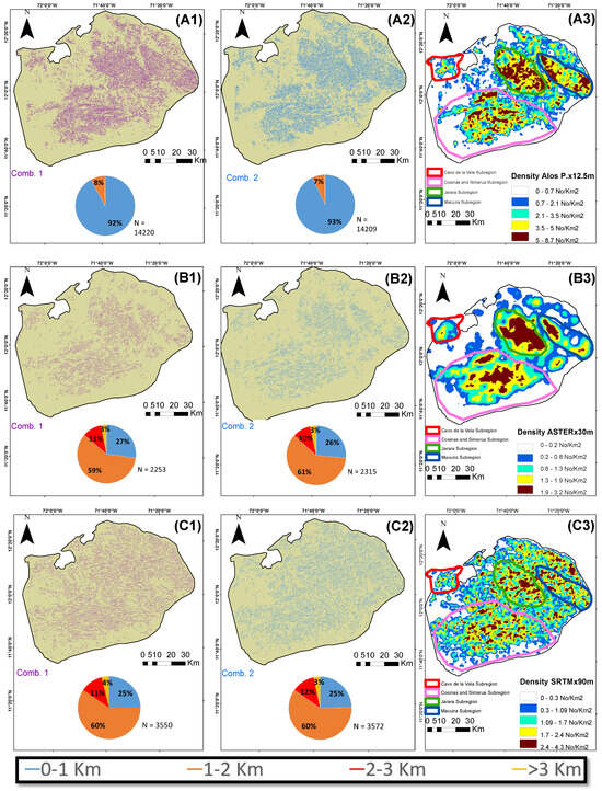
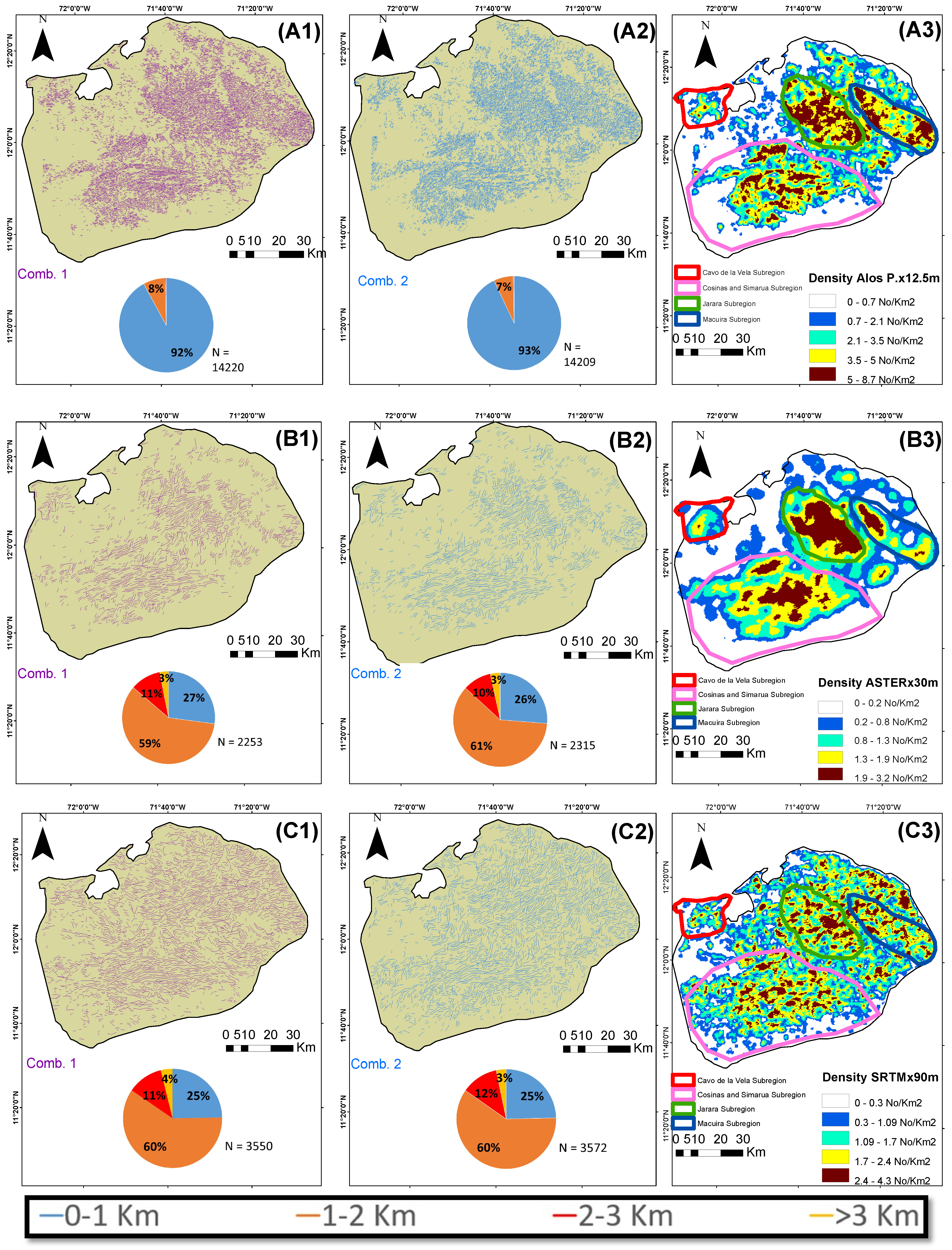
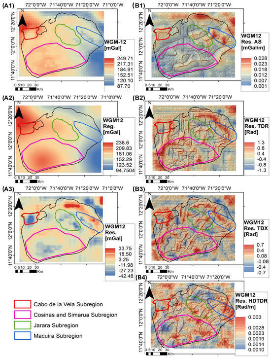
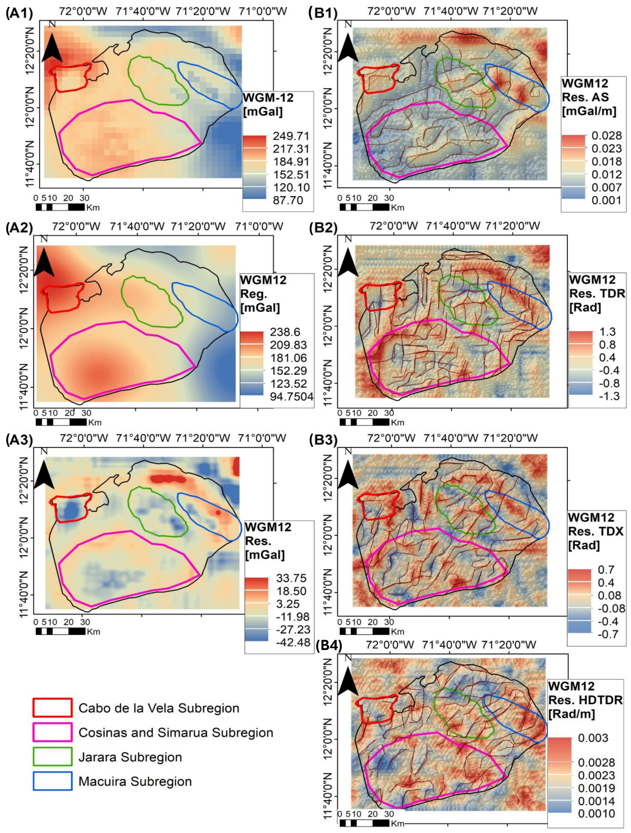
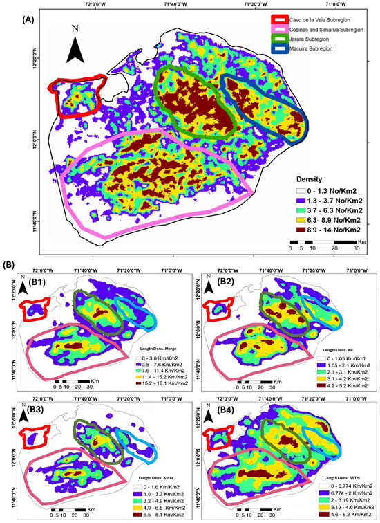
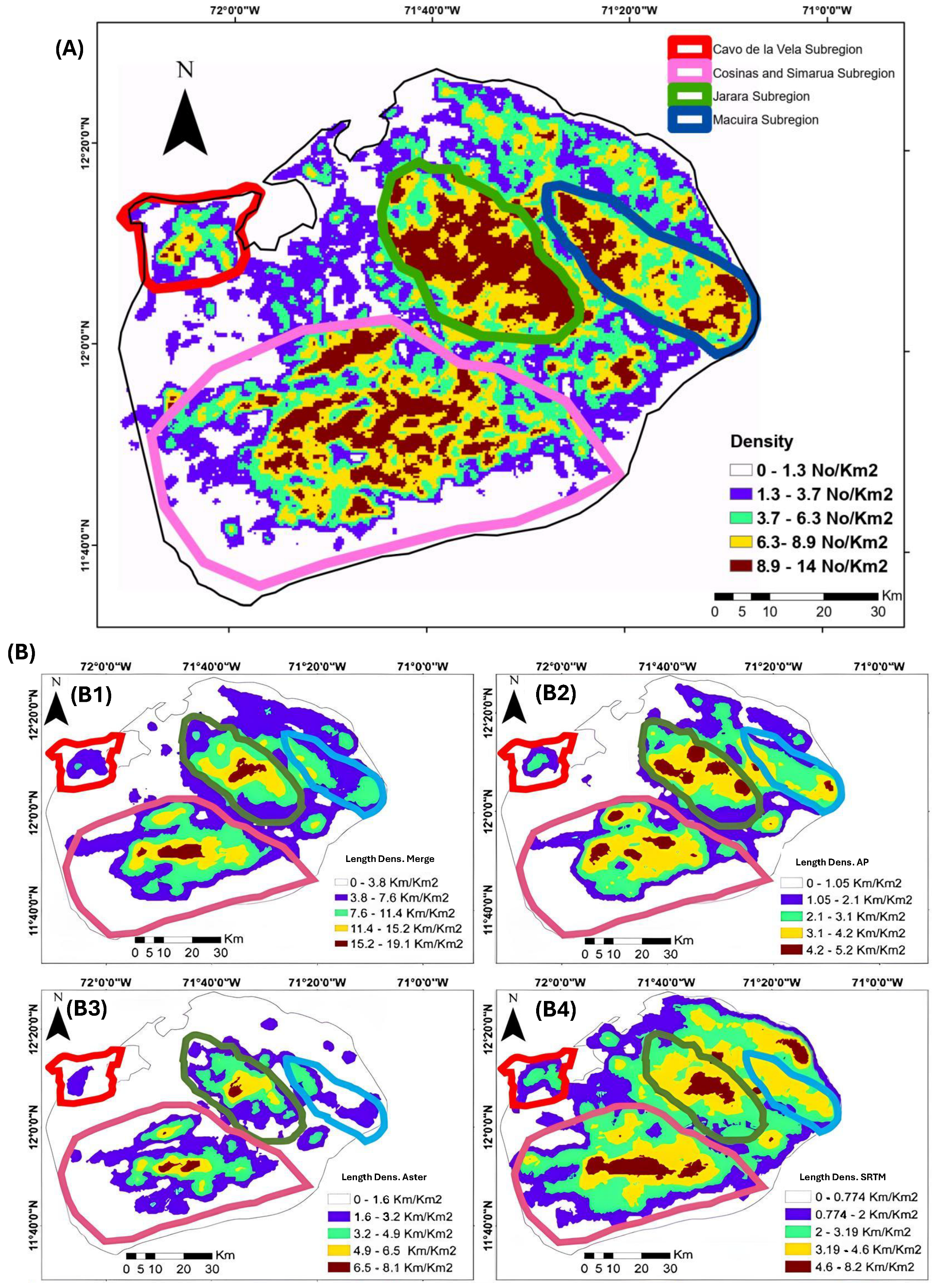
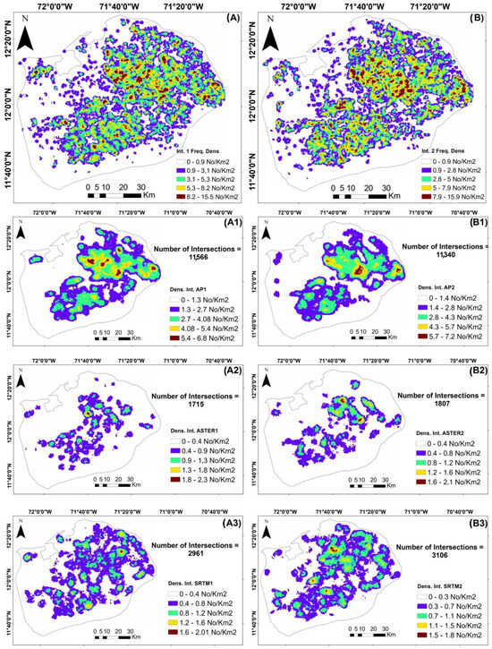
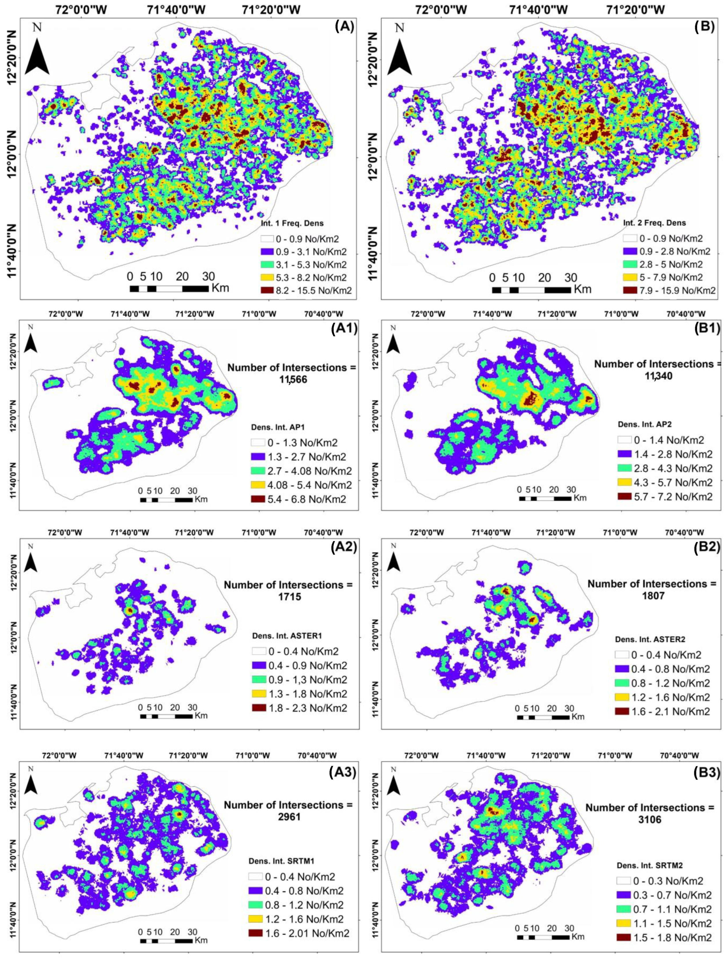
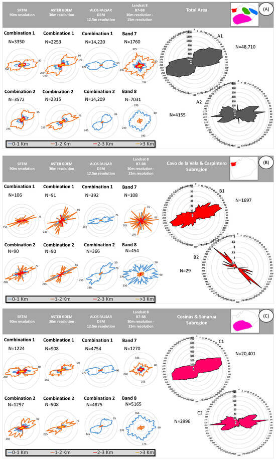
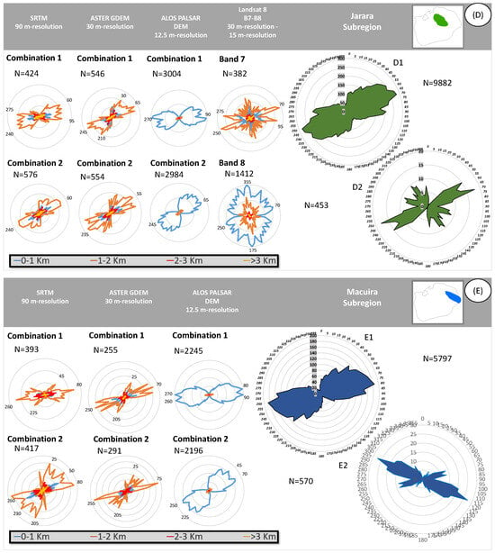
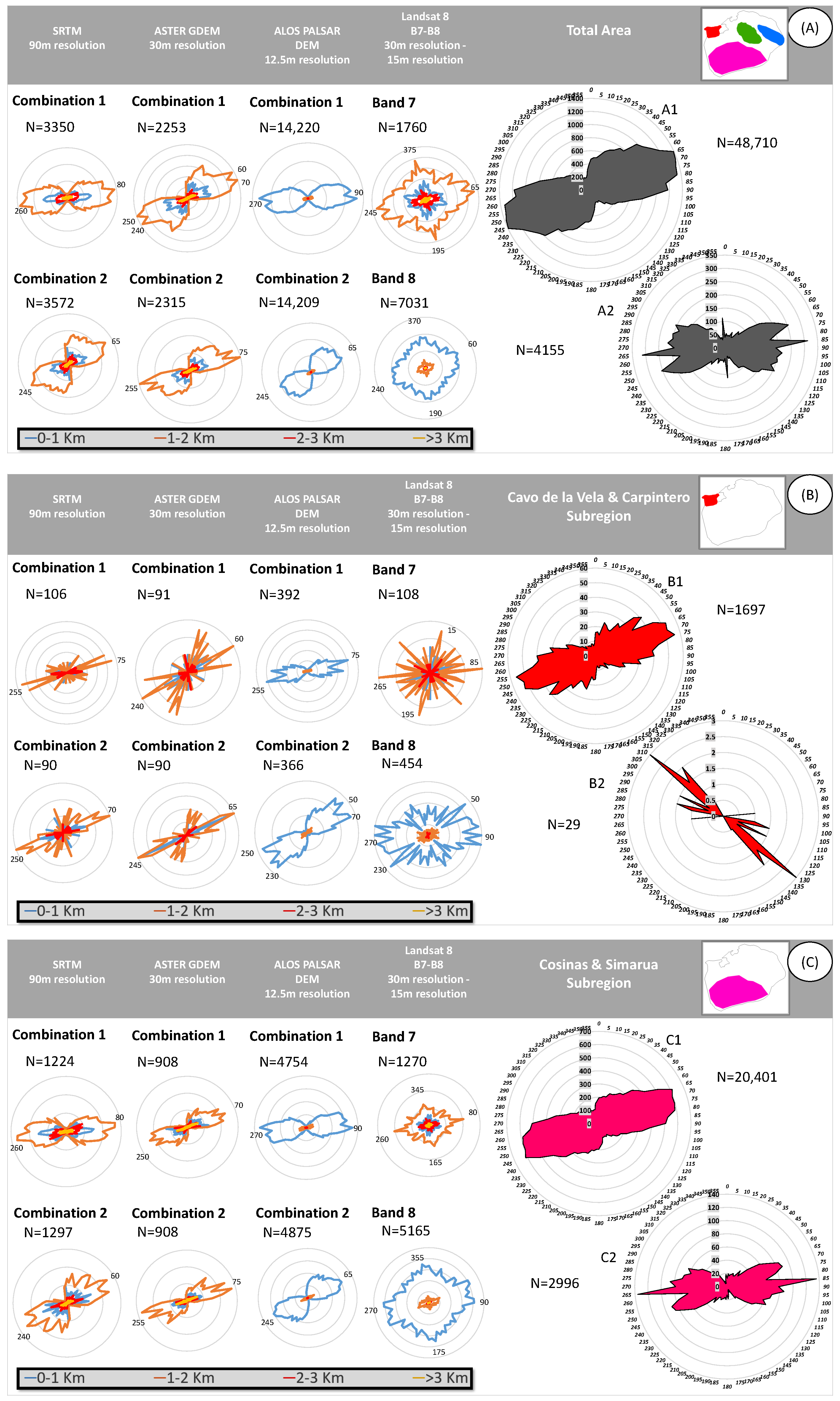
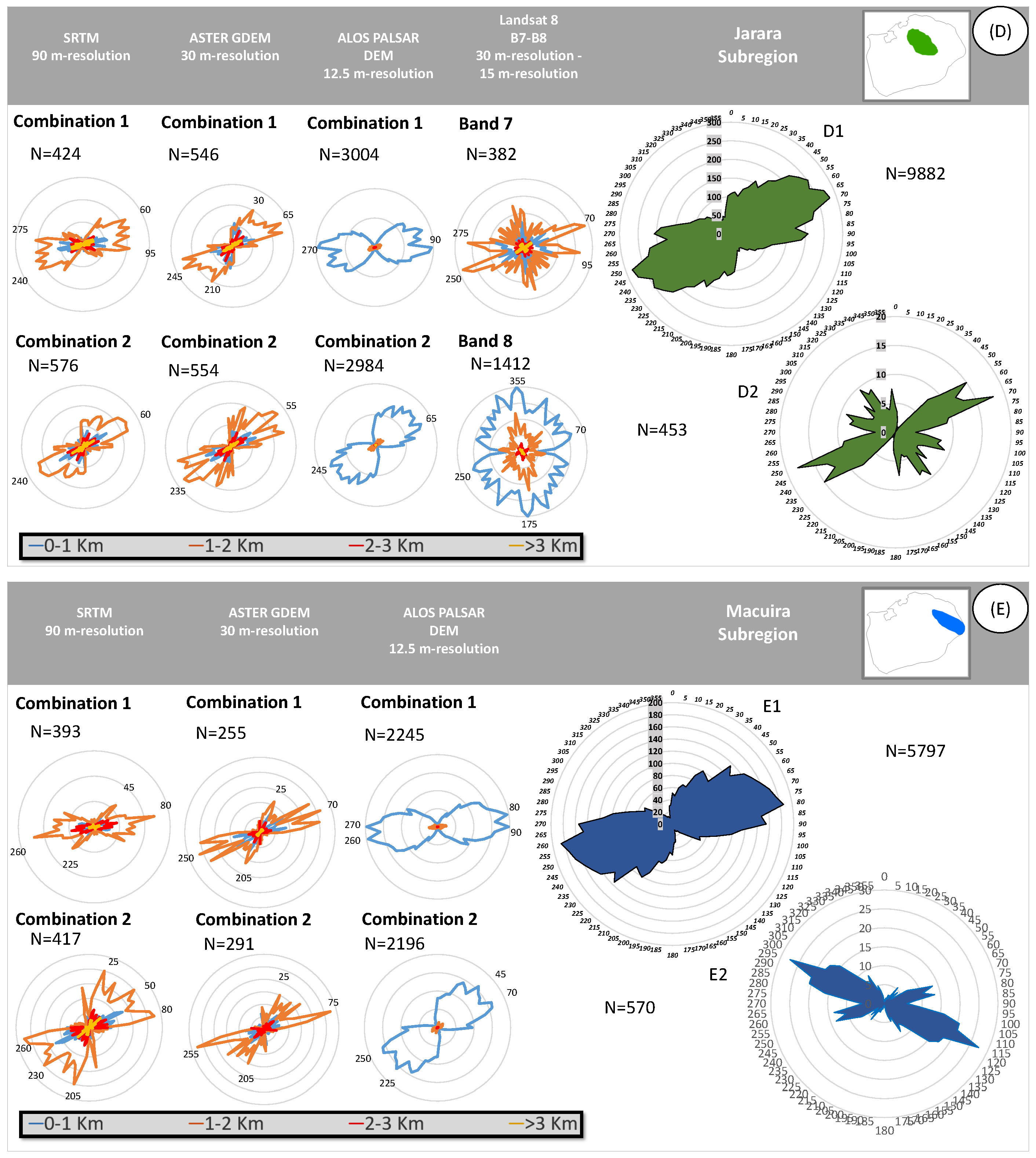
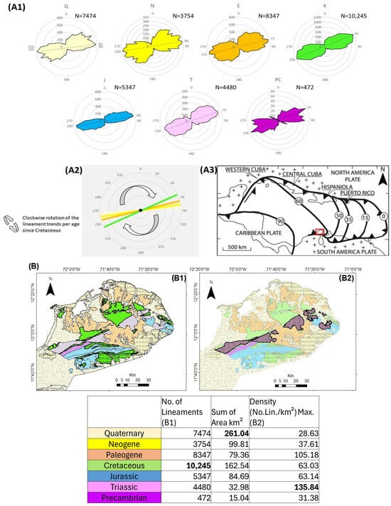
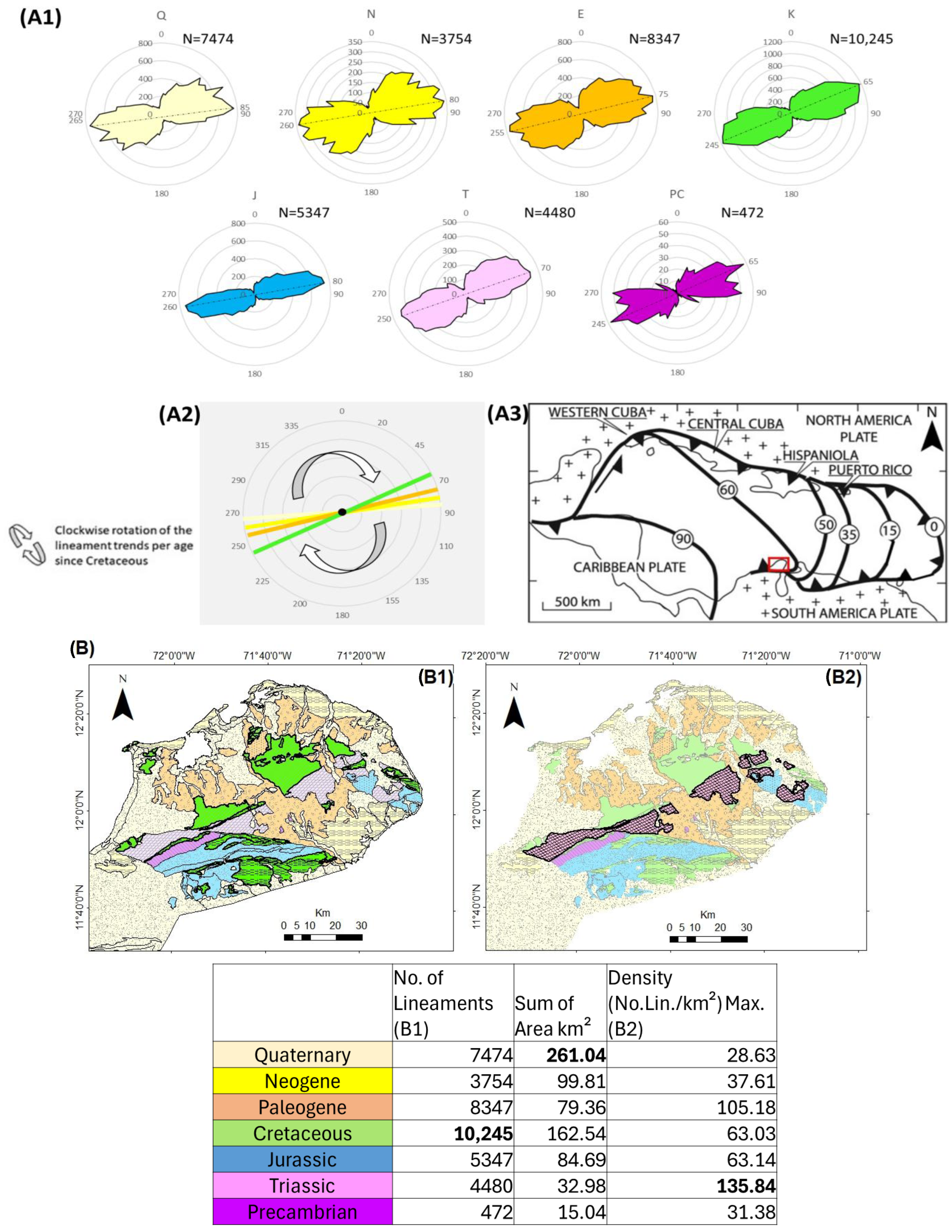
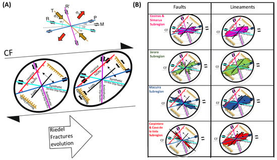
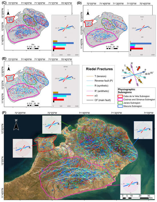
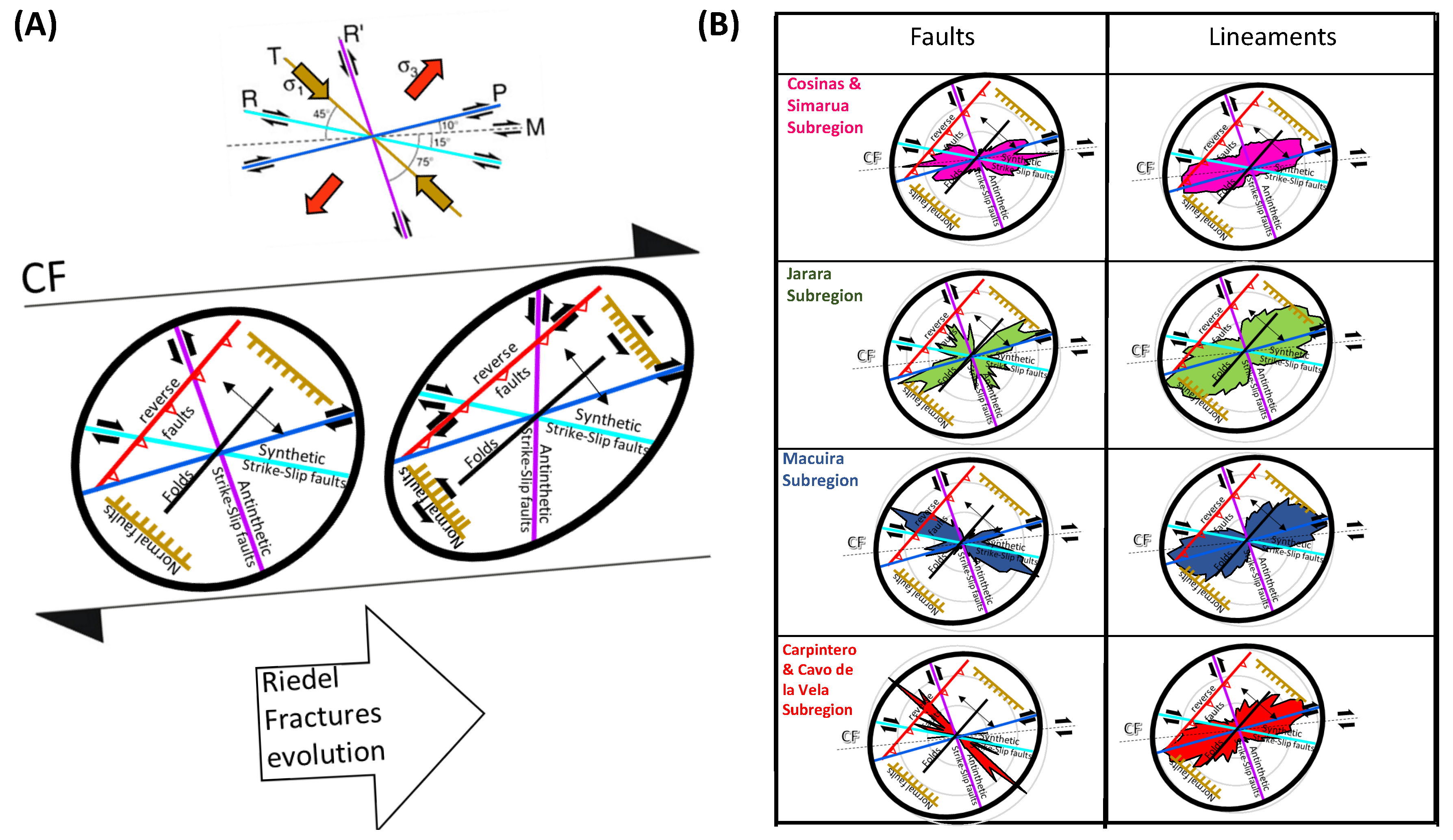
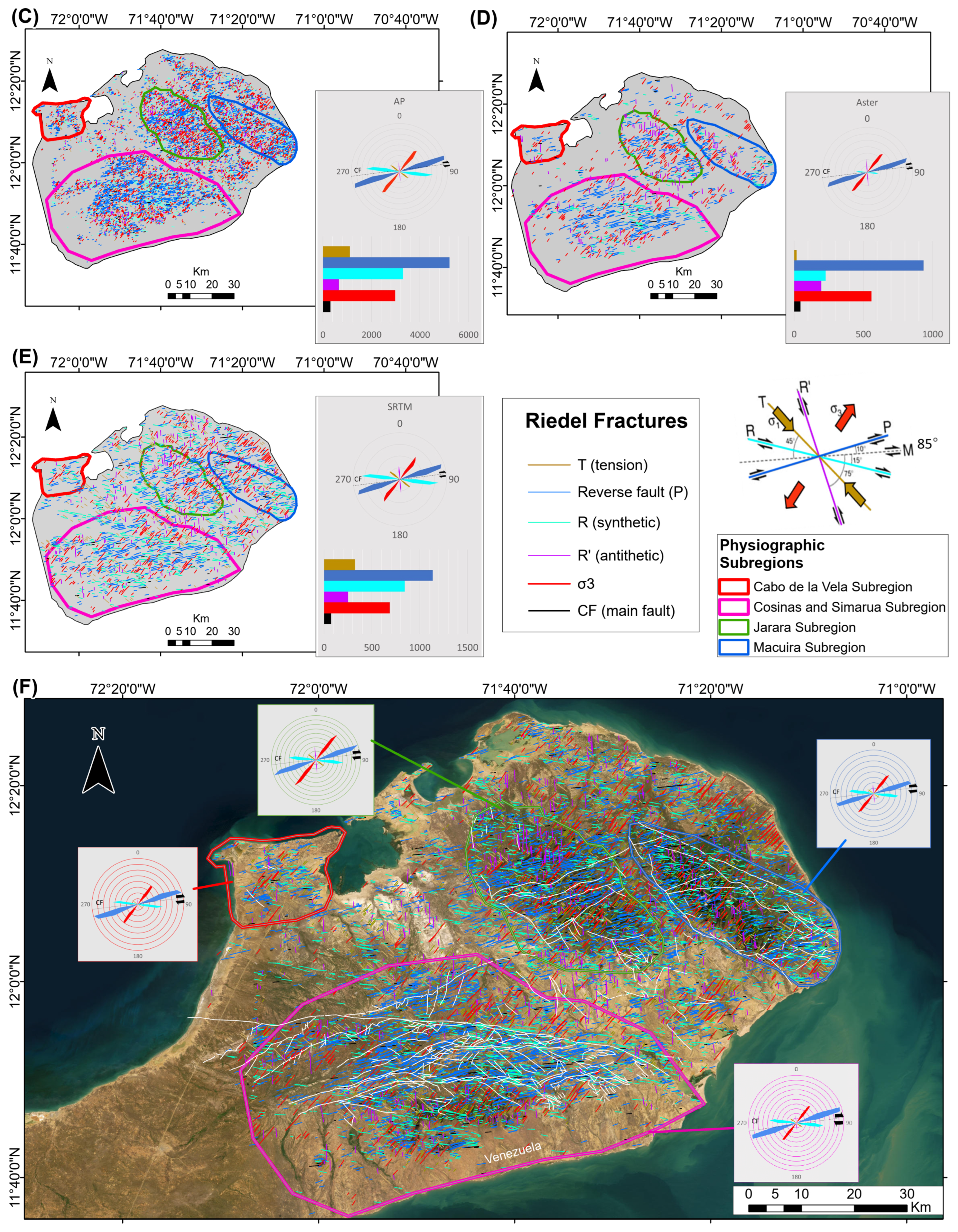
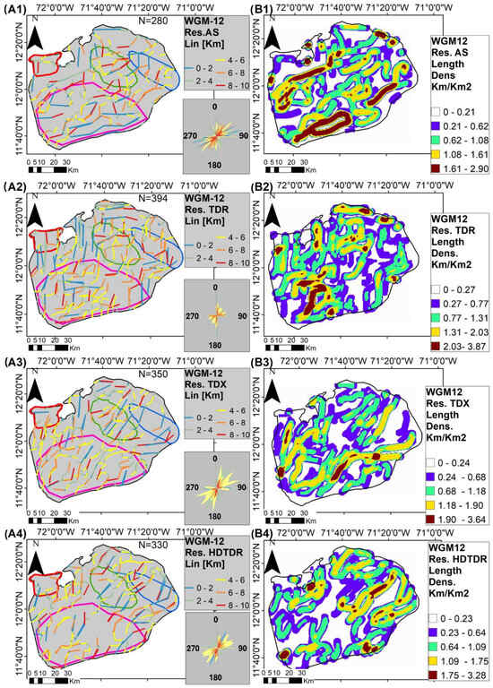
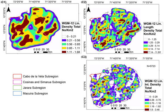
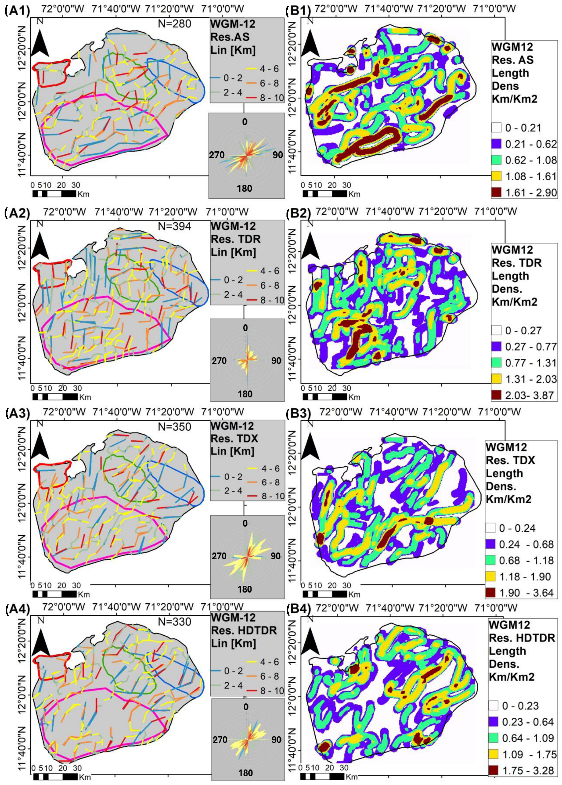
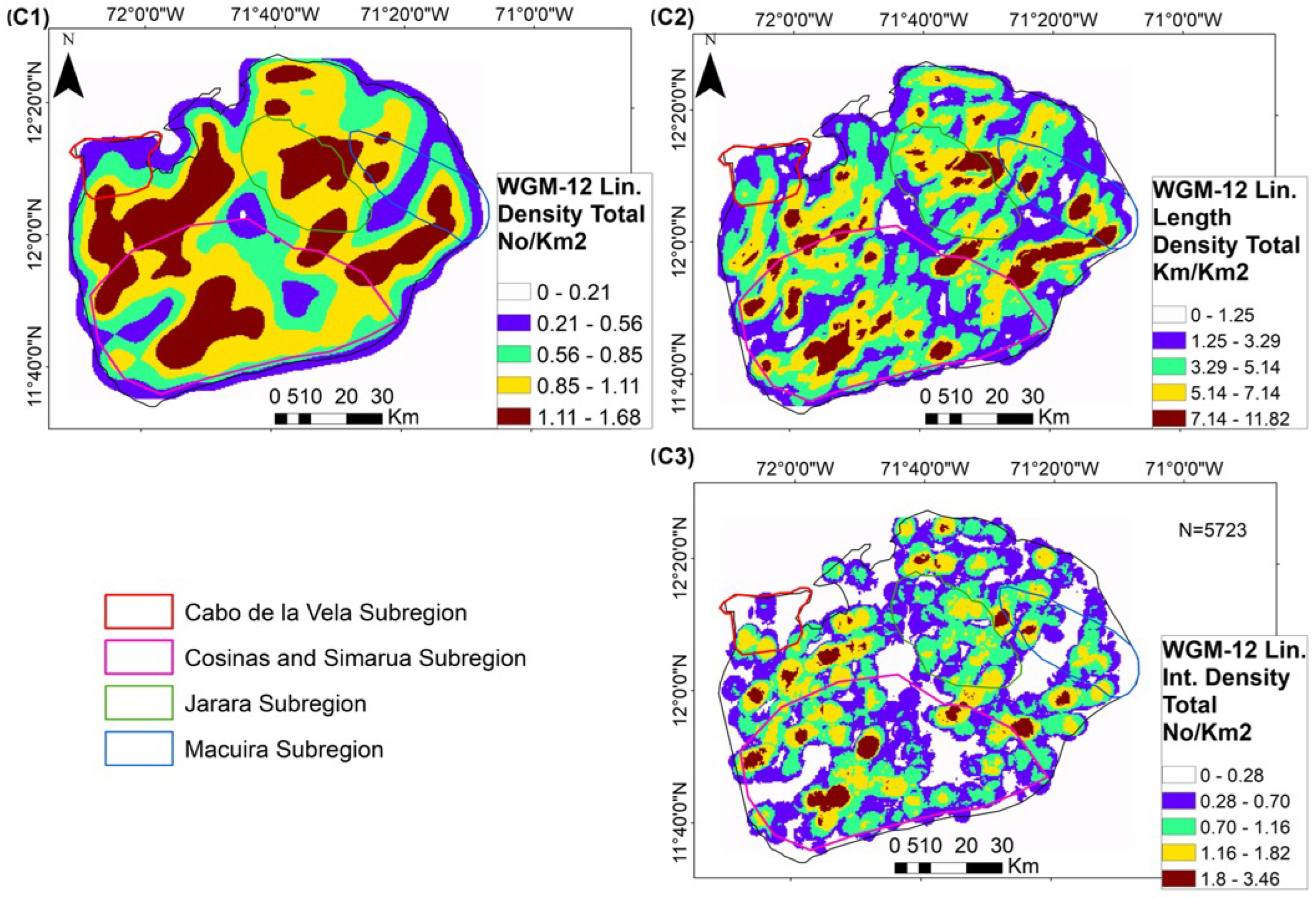
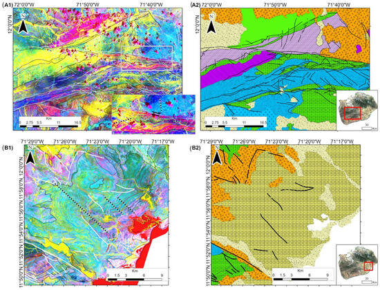
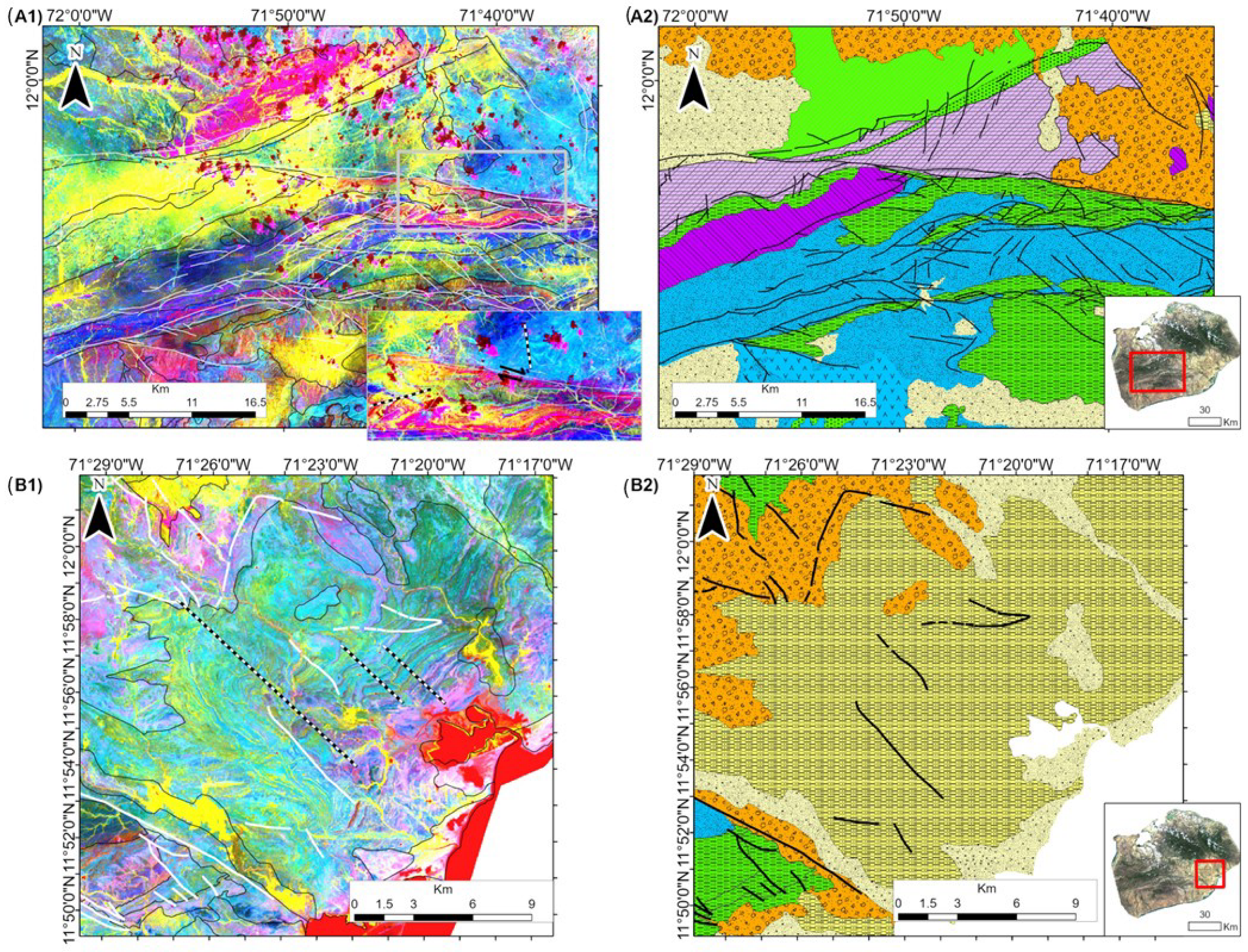
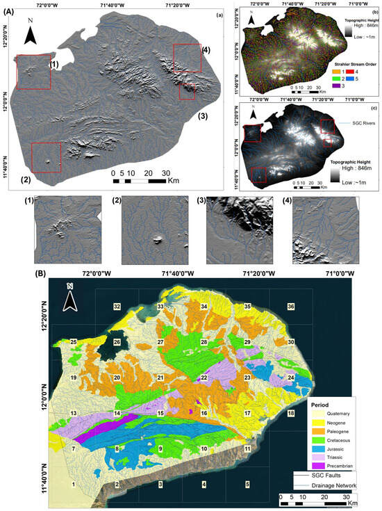
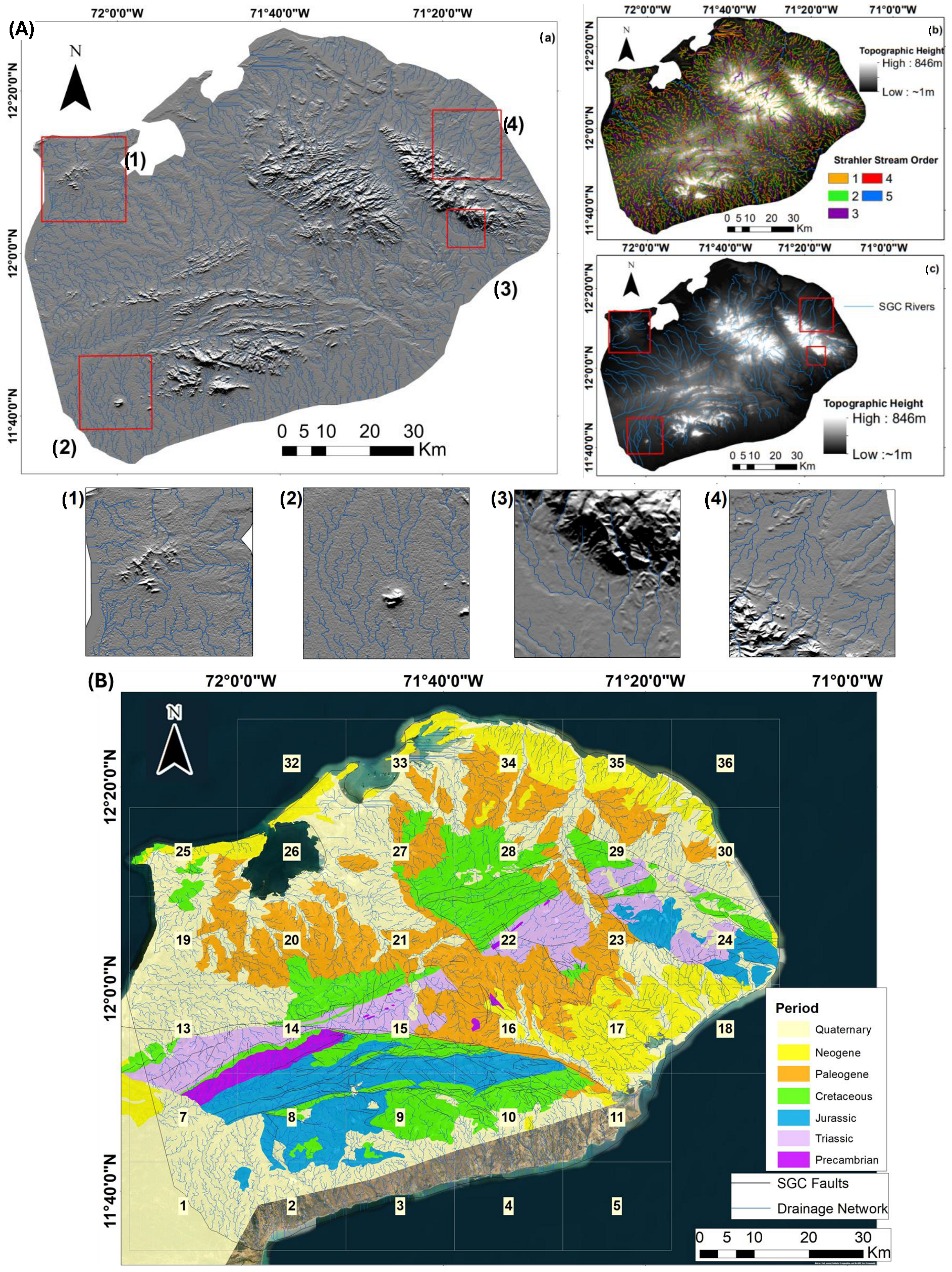
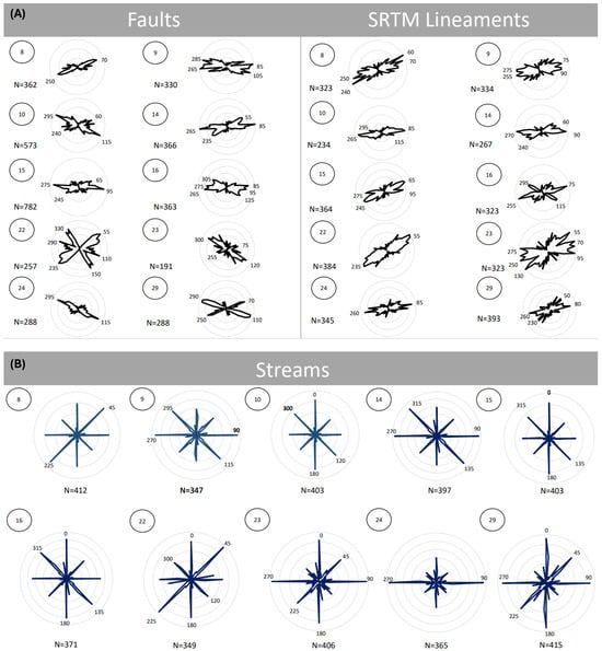
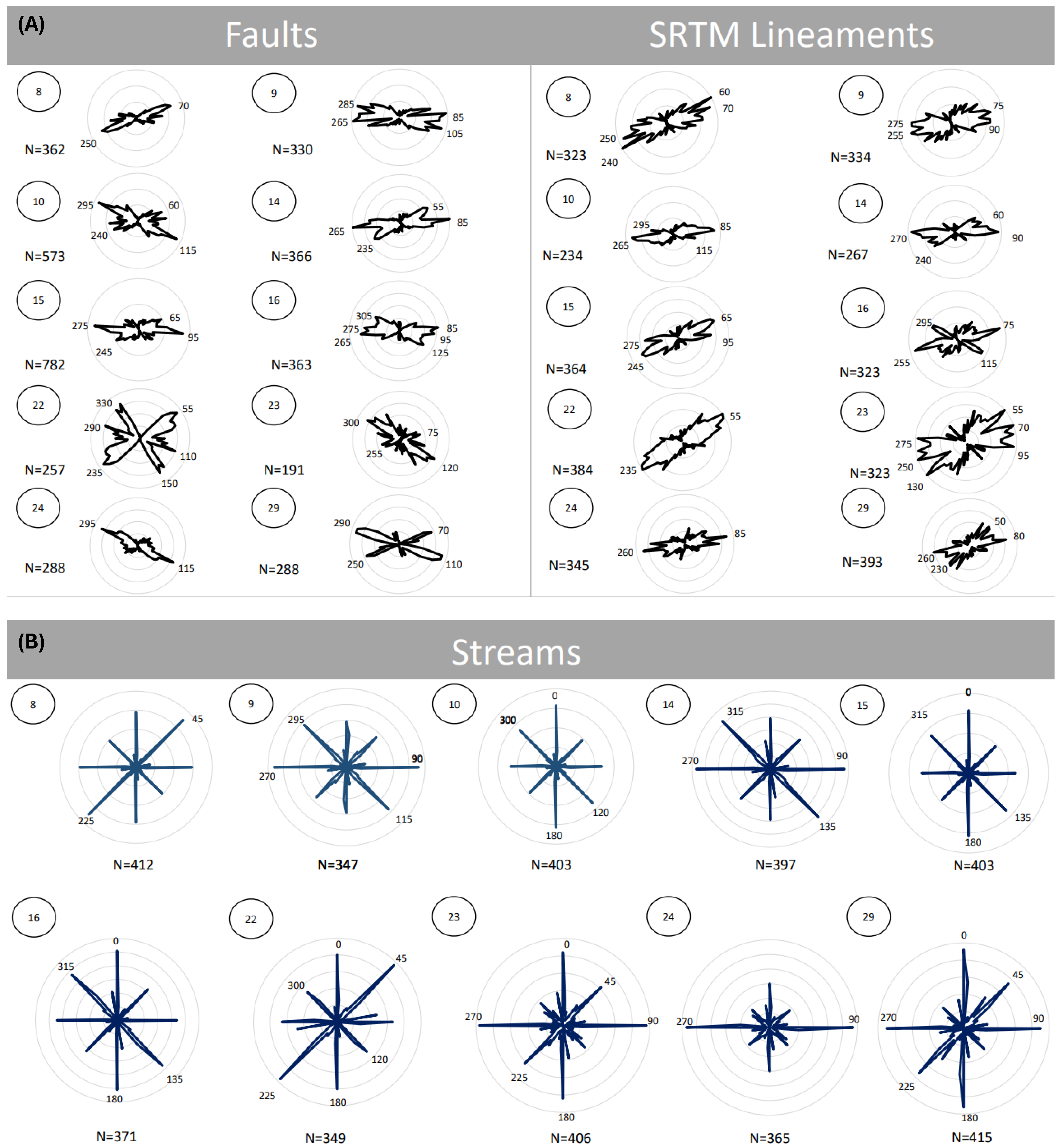
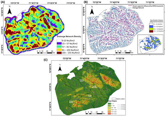
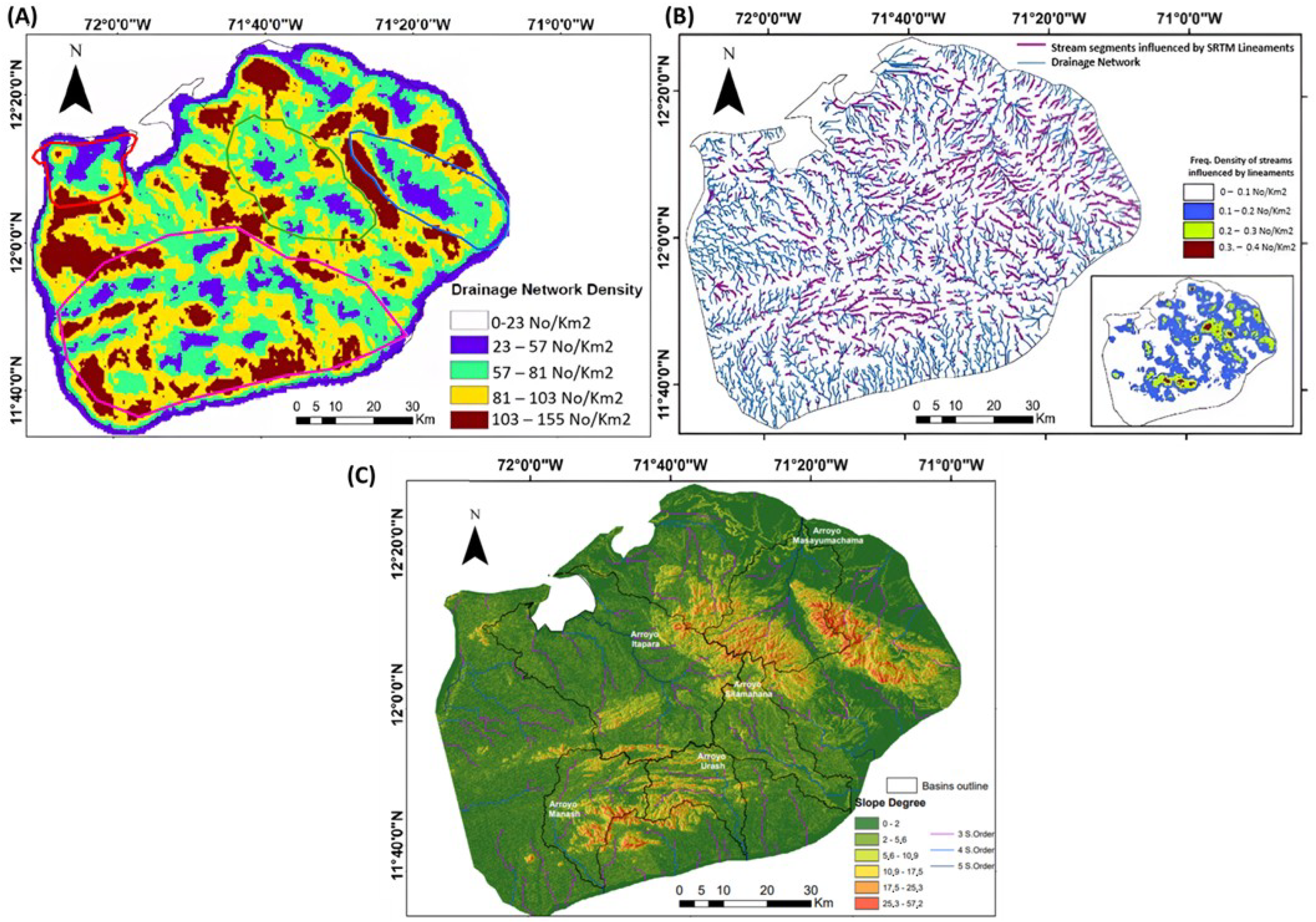

Disclaimer/Publisher’s Note: The statements, opinions and data contained in all publications are solely those of the individual author(s) and contributor(s) and not of MDPI and/or the editor(s). MDPI and/or the editor(s) disclaim responsibility for any injury to people or property resulting from any ideas, methods, instructions or products referred to in the content. |
© 2026 by the authors. Licensee MDPI, Basel, Switzerland. This article is an open access article distributed under the terms and conditions of the Creative Commons Attribution (CC BY) license.