Analysis of Pre-Seismic Disturbances Based on Dynamic Variations in Gravity Solid Tide Amplitude Factors

Abstract

Pre-seismic anomalies in solid tidal factors can reveal crustal stress accumulation and predict seismic risk; such disturbance signals associated with earthquake incubation are extremely subtle and easily obscured by environmental noise, instrument errors, and other interference factors, placing heightened demands on the precision of gravity data acquisition and the capability to detect and isolate solid tidal signals effectively. In this paper, we propose a novel method for determining time-varying solid tidal factors based on the normal time–frequency transform (NTFT) theory, an approach allowing us to unbiasedly determine the instantaneous amplitude, frequency, and phase of time-varying signals, while mitigating the influence of edge effects to a certain extent. In the study outlined in this paper, we first design simulation experiments to validate the effectiveness of the new method. Subsequently, utilising high-precision superconducting gravimeter observation data, the proposed method is applied to the detection of pre-seismic disturbances preceding the 2004 Sumatra megathrust earthquake. Our results demonstrate that, compared to traditional harmonic analysis methods, this novel approach more accurately filters out interference signals, effectively captures the faint pre-seismic perturbations of solid tides, and significantly enhances the timeliness of pre-seismic disturbance detection, thus providing more reliable technical support for earthquake precursor monitoring.

1. Introduction

The core value of detecting pre-earthquake disturbances lies in providing direct observational evidence for analysing earthquake genesis mechanisms [1,2], while offering scientific support for seismic risk prediction and pre-earthquake early warning [3,4]. Accurate capture and analysis of pre-earthquake disturbance characteristics constitute crucial prerequisites for overcoming scientific bottlenecks in earthquake prediction, as well as enhancing regional seismic disaster prevention capabilities [5,6,7]; this holds irreplaceable significance for deepening our understanding of Earth’s internal dynamics and safeguarding geological security [8]. In this paper, we present a novel method for determining the time-varying amplitude factors of solid Earth tides; through cross-validation with multiple earthquake cases, we confirm the existence of anomalous disturbances in the amplitude factors of the Q1 tidal waves prior to both the 2004 Sumatra earthquake and the 2010 Chile earthquake.

Currently, the widely adopted software for determining global gravity solid tidal amplitude factors includes Venedikov (VAV), Eterna, Baytap-G&L, and Tsoft [9,10,11,12], programmes which were developed based on tidal theory and harmonic analysis methods, exhibiting strong dependence on prior parameters, demanding high-quality and lengthy observational data, and demonstrating poor adaptability to non-stationary signals [13,14,15]. The constants determined through harmonic analysis essentially represent the (weighted) average of the time-varying amplitudes of each component tidal wave within a specific time window [16], rather than the state of each component tidal wave at every instant.

The frequency resolution of harmonic analysis is closely tied to data length. Taking the K1 and P1 waves, whose frequencies are relatively close, as an example, determining their harmonic constants with high precision requires at least ${\left(f_1-f_2\right)}^{-1}={(f_{K_1}-f_{P_1})}^{-1}\approx 182.65$ days of data, indicating that harmonic analysis cannot meet the requirements for analysing the dynamic variations in component amplitude factors. Even studies sacrificing harmonic parameter precision can only achieve a monthly timescale resolution [17], rendering harmonic analysis unsuitable for seismic precursor monitoring.

Despite the temporal resolution limitations of harmonic analysis, the dynamic variations in amplitude factors have been demonstrated to correlate closely with seismic activity; some scholars, through systematic review of historical seismic observation cases, propose that, when amplitude factors exhibit abnormal fluctuations exceeding 3%, there exists a potential for a magnitude 6 or greater earthquake occurring in the vicinity of the corresponding station [18], a research conclusion which demonstrates that subtle variations in amplitude factor serve as key characteristic indicators for identifying pre-seismic disturbance signals, providing crucial theoretical grounding for earthquake precursor monitoring [19,20,21]. Owing to their substantial energy contents, the M2 and O1 tidal waves have been extensively selected as subjects in prior amplitude factor studies [22,23,24,25,26]. Meanwhile, Q1 is a weak lunar diurnal tidal constituent (one order lower than O1), arising from orbital ellipticity, whose small amplitude and proximity to other diurnal modes make it difficult to extract; however, experimental studies have shown that, compared to the M2 and O1 tidal constituents, the Q1 tidal wave may be more sensitive to subtle changes in Earth’s elastic response. Therefore, in this study, the Q1 tidal constituent was selected as the research subject.

In order to achieve a refined characterisation of the dynamic variations in amplitude factors, there is an urgent need to develop analytical methods with higher temporal resolution; such methods would enable the determination of amplitude factor parameters using fewer data samples, thereby capturing potential disturbance signals within a shorter pre-seismic time window and providing support for the precise identification of pre-seismic disturbances. Accordingly, we propose a novel method for extracting time-varying signals, through an approach which enables unbiased determination of the instantaneous amplitude, frequency, and phase of time-varying signals, thereby effectively revealing the dynamic evolution patterns of tidal factors; building upon this foundation, we focus on analysing the pre-seismic disturbance characteristics of the Q1 tidal wave, aiming to overcome the reliance of traditional research on specific tidal waves, thereby offering new technical pathways and research perspectives for pre-seismic disturbance detection.

2. Method for Determining Dynamic Amplitude Factors

2.1. Normal Time–Frequency Transform (NTFT) Theory

For time-varying signals, both temporal and frequency domain characteristics must be considered concurrently. In 2007, Liu Lintao introduced the concept of the normal time–frequency transform (NTFT), which enables unbiased determination of a signal’s instantaneous period, amplitude, and phase [14,27,28,29,30]. A brief overview of this theory follows.

The normal time–frequency transform of the function $f(t)\in L^1(R)$ is defined as follows:

$$\mathrm{\Psi }f(\tau ,\varpi )={\displaystyle {\int }_{R}f(t)\overline{\psi (t-\tau ,\varpi )}\mathrm{d}t,\tau ,\varpi \in R}$$

(1)

where $\tau$ denotes the time factor, $\varpi$ denotes the frequency factor, the superscript “-” denotes the conjugate operator, and $\psi \left(t,\varpi \right)$ denotes the kernel function. In the definition of the normal time–frequency transform, the kernel function should satisfy the following condition:

$$\widehat{\psi }(\omega ,\varpi )={\displaystyle {\int }_R\psi }(t,\varpi )\exp (-i\varpi t)dt\dot{\ne }0$$

(2)

where “$\cdot$” denotes almost everywhere.

The kernel function adopted for this paper is as follows:

$$\psi (t,\varpi )=\left|\varpi \right|w(\varpi t)\exp (i\varpi t),(\varpi \in R)\dot{\ne }0$$

(3)

where $w\left(t\right)$ denotes the standard Gaussian window function.

$$w(t)={\displaystyle \frac{1}{\sqrt{2\pi }\sigma }}\exp (-{\displaystyle \frac{t^2}{2{\sigma }^2}}),\sigma >0$$

(4)

where $\sigma$ denotes the Gaussian window width parameter.

For a harmonic signal, $h\left(t\right)=A\exp \left(i\beta t+i\phi \right)$, where $A\in {\mathrm{R}}^{+}$ is the signal amplitude, $\beta$ is the angular frequency, and $\phi$ is the initial phase, through which it can be demonstrated that its NTFT satisfies the following:

$$\left|\mathsf{\Psi }h\left(\tau ,\varpi \right)\right|=\mathrm{Maximum}\iff \varpi =\beta ,\forall \tau \in R$$

(5)

$$\mathsf{\Psi }h\left(\tau ,\beta \right)=h\left(\tau \right)=\left|A\right|\exp \left(i\beta \tau +i\phi \right),\forall \tau \in R$$

(6)

With Equation (5), we demonstrate that the NTFT can be used to unbiasedly determine instantaneous frequency, while Equation (6) shows that it can also be used to unbiasedly determine the instantaneous amplitude and phase, two relationships that theoretically guarantee that the NTFT can be used to unbiasedly determine the instantaneous amplitude, frequency, and phase.

2.2. Non-Reconstruction NTFT Theory

Assume that a multi-component signal $f\left(t\right)$ is composed of $N$ frequency components, $h_n\left(t\right)=A_n\exp \left(i{\varpi }_{n}t+i{\beta }_n\right)$.

$$f\left(t\right)={\displaystyle \sum _{n=1}^N{h}_n\left(t\right)=}{\displaystyle \sum _{n=1}^N{A}_n\exp \left(i{\varpi }_{n}t+i{\beta }_n\right)}$$

(7)

The normal time–frequency transform of a multi-component signal $f\left(t\right)$ is as follows:

$$\mathsf{\Psi }f\left(\tau ,\varpi \right)={\displaystyle \sum _{n=1}^N\overline{\widehat{\psi }}\left({\varpi }_n,\varpi \right)}{h}_n\left(\tau \right)={\displaystyle \sum _{n=1}^N\overline{\widehat{w}}\left(\frac{{\varpi }_n-\varpi }{\mu \left(\varpi \right)}\right)}{h}_n\left(\tau \right)$$

(8)

where $\overline{\widehat{\psi }}\left(\omega ,\varpi \right)$ is termed the harmonic amplitude weight (HAW) [31].

From the normal time–frequency transform of a multicomponent signal (Equation (8)), it can be seen that, in order to separate the component signals, the parameters of the normal time–frequency transform must be adjusted so that the harmonic amplitude weight of the NTFT satisfies the following:

$$E_{\psi }\left({\varpi }_i,{\varpi }_j\right)=\left\{\begin{array}{cc}\begin{array}{c}1\\ 0\end{array}\hfill & \begin{array}{c}i=j\\ i\ne j\end{array}\hfill \end{array}\right.$$

(9)

When $\varpi ={\varpi }_1,{\varpi }_2,\cdots {\varpi }_n$, the normal time–frequency transform coefficients $\mathsf{\Psi }f\left(\tau ,{\varpi }_i\right)$ and $i=1,2,\cdots n$ represent the respective component signals. The properties of the standard window function (Equation (2)) ensure that the elements on the diagonal of the harmonic amplitude weight matrix equal 1. To satisfy the requirement that the off-diagonal data of the harmonic amplitude weight matrix $W$ approaches 0, a sufficiently long time domain window width must be set; correspondingly, the influences of edge effects are also significant, reducing the timeliness of time–frequency analysis.

To address this issue, Su Xiaoqing [31] proposed a non-reconstruction NTFT algorithm in 2014, which mitigates edge effects to some extent, while maintaining frequency resolution requirements. Performing a normal time–frequency transform on the multicomponent signal (Equation (7)), and identifying the frequency of each component signal through the NTFT spectrum, yields ${\varpi }_n$($n=1,2,\cdots ,N$). Substituting ${\varpi }_n$ into the normal time–frequency transform of the multicomponent signal (Equation (8)) yields the following system of equations:

$$\left\{\begin{array}{c}\mathsf{\Psi }h\left(\tau ,{\varpi }_1\right)=h_1\left(\tau \right)+\overline{\widehat{w}}\left({\displaystyle \frac{{\varpi }_2-{\varpi }_1}{\mu \left({\varpi }_1\right)}}\right)h_2\left(\tau \right)+\cdots +\overline{\widehat{w}}\left({\displaystyle \frac{{\varpi }_n-{\varpi }_1}{\mu \left(\varpi 1\right)}}\right)h_n\left(\tau \right)\\ \mathsf{\Psi }h\left(\tau ,{\varpi }_2\right)=\overline{\widehat{w}}\left({\displaystyle \frac{{\varpi }_1-{\varpi }_2}{\mu \left({\varpi }_2\right)}}\right)h_1\left(\tau \right)+h_2\left(\tau \right)+\cdots +\overline{\widehat{w}}\left({\displaystyle \frac{{\varpi }_n-{\varpi }_2}{\mu \left({\varpi }_2\right)}}\right)h_n\left(\tau \right)\\ ⋮\\ \mathsf{\Psi }h\left(\tau ,{\varpi }_n\right)=\overline{\widehat{w}}\left({\displaystyle \frac{{\varpi }_1-{\varpi }_n}{\mu \left({\varpi }_n\right)}}\right)h_1\left(\tau \right)+\overline{\widehat{w}}\left({\displaystyle \frac{{\varpi }_2-{\varpi }_n}{\mu \left({\varpi }_n\right)}}\right)h_2\left(\tau \right)+\cdots +h_n\left(\tau \right)\end{array}\right.$$

(10)

To simplify the expression, the following three variables are introduced:

$$T=\left[\begin{array}{c}\mathsf{\Psi }h\left(\tau ,{\varpi }_1\right)\\ \mathsf{\Psi }h\left(\tau ,{\varpi }_2\right)\\ ⋮\\ \mathsf{\Psi }h\left(\tau ,{\varpi }_n\right)\end{array}\right], E=\left[\begin{array}{c}{h}_1\left(\tau \right)\\ h_2\left(\tau \right)\\ ⋮\\ h_n\left(\tau \right)\end{array}\right], W=\left[\begin{array}{cccc}1& \overline{\widehat{w}}\left({\displaystyle \frac{{\varpi }_2-{\varpi }_1}{\mu \left({\varpi }_1\right)}}\right)& \cdots & \overline{\widehat{w}}\left({\displaystyle \frac{{\varpi }_n-{\varpi }_1}{\mu \left(\varpi 1\right)}}\right)\\ \overline{\widehat{w}}\left({\displaystyle \frac{{\varpi }_1-{\varpi }_2}{\mu \left({\varpi }_2\right)}}\right)& 1& \cdots & \overline{\widehat{w}}\left({\displaystyle \frac{{\varpi }_n-{\varpi }_2}{\mu \left({\varpi }_2\right)}}\right)\\ ⋮& ⋮& ⋮& ⋮\\ \overline{\widehat{w}}\left({\displaystyle \frac{{\varpi }_1-{\varpi }_n}{\mu \left({\varpi }_n\right)}}\right)& \overline{\widehat{w}}\left({\displaystyle \frac{{\varpi }_2-{\varpi }_n}{\mu \left({\varpi }_n\right)}}\right)& \cdots & 1\end{array}\right]$$

Thus, the matrix form of Equation (9) is as follows:

$$T=WE$$

(11)

where $T$ denotes the NTFT coefficient vector; $E$ represents the respective subcomponents; and $W$ denotes the harmonic amplitude weight matrix.

Solving this system of equations yields the following individual subcomponents:

$$E=W^{-1}T$$

(12)

Through Equation (12), it can be observed that the non-reconstructive algorithm imposes fewer requirements on the non-diagonal elements of the harmonic amplitude weight matrix $W$; these elements need not approach zero, as it suffices to ensure that the matrix remains invertible to recover the individual component signals. Consequently, the time-domain window width may be appropriately reduced, thereby diminishing the impacts of edge effects. Therefore, this algorithm effectively reconciles the trade-off between frequency resolution and edge effects, maintaining frequency resolution while mitigating the impacts of edge effects to a certain extent.

2.3. Amplitude Factor Calculation Method

The amplitude factor is defined as the ratio of the measured gravity solid tide amplitude to the amplitude corresponding to the theoretical gravitational tidal force, reflecting the amplification or attenuation effect of Earth deformation on gravitational tidal forces, as follows:

$$\delta ={\displaystyle \frac{A_{obs}}{A_{theo}}}$$

(13)

where $A_{obs}$ denotes the amplitude of the measured gravity solid tide signal, and $A_{theo}$ represents the theoretical tidal force amplitude for the corresponding tidal component. For an ideal rigid Earth, $\delta =1$; however, due to elastic deformation in the actual Earth, $\delta$ is typically slightly greater than 1 (approximately 1.16).

Theoretical values for gravitational solid tidal components are calculated using the Tamura tidal table, a high-precision tidal generating potential harmonic expansion table, released by Japanese scholar Tamura in 1987 and 1995, providing core fundamental data for tidal analysis, as well as marine and geophysical research [32,33], for core parameters, combined with harmonic analysis methods. Based on the preset parameters for the i-th tidal component in the Tamura tidal table, a theoretical signal model for that component is constructed, expressed as follows:

$$g_i(t)=f_i\cdot G_i\cdot \cos ({\omega }_{i}t+{\phi }_i-u_i)$$

(14)

where $g_i(t)$ denotes the theoretical gravitational value of the i-th component tide at time t; $f_i$ and $u_i$ represent the intersection factor and intersection correction angle, respectively, for this component tide (derived from the Tamura tide table to correct for orbital variations affecting the component tide); $G_i$ is the theoretical amplitude of this component tide (sourced from the Tamura tidal wave table based on global or regional tidal models); ${\omega }_i$ denotes the angular velocity of the tidal wave; and ${\phi }_i$ represents the theoretical initial phase of this tidal wave (taken from the Tamura tidal wave table, associated with the longitude of the observation point).

3. Simulation Validation

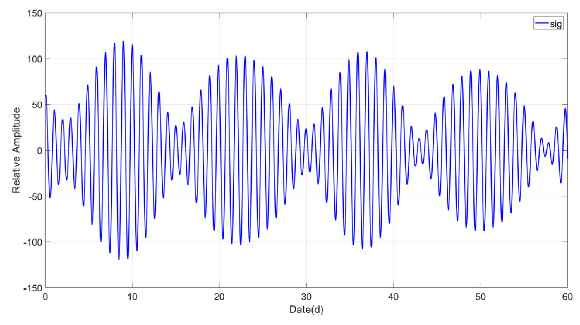
Using the relative amplitude and period information of the four component tides K1, O1, P1, and Q1, a 60-day solid tidal daily simulation signal was constructed, as follows:

$$\begin{array}{l}sig= 54.4\times A(t)\times \cos \left({\displaystyle \frac{2\pi }{23.9345}}\times t+{\phi }_1\right)+7.9\times A(t)\times \cos \left({\displaystyle \frac{2\pi }{26.8684}}\times t+{\phi }_2\right)\\ +41.5\times A(t)\times \cos \left({\displaystyle \frac{2\pi }{25.8193}}\times t+{\phi }_3\right)+19.3\times A(t)\times \cos \left({\displaystyle \frac{2\pi }{24.0659}}\times t+{\phi }_4\right)\end{array}$$

(15)

where $A(t)$ represents a time-varying amplitude with an approximate variation of 3%, and ${\phi }_1\sim {\phi }_4$ denotes the random phase. The simulated signal is depicted in Figure 1, with the blue line illustrating the amplitude variation over time.

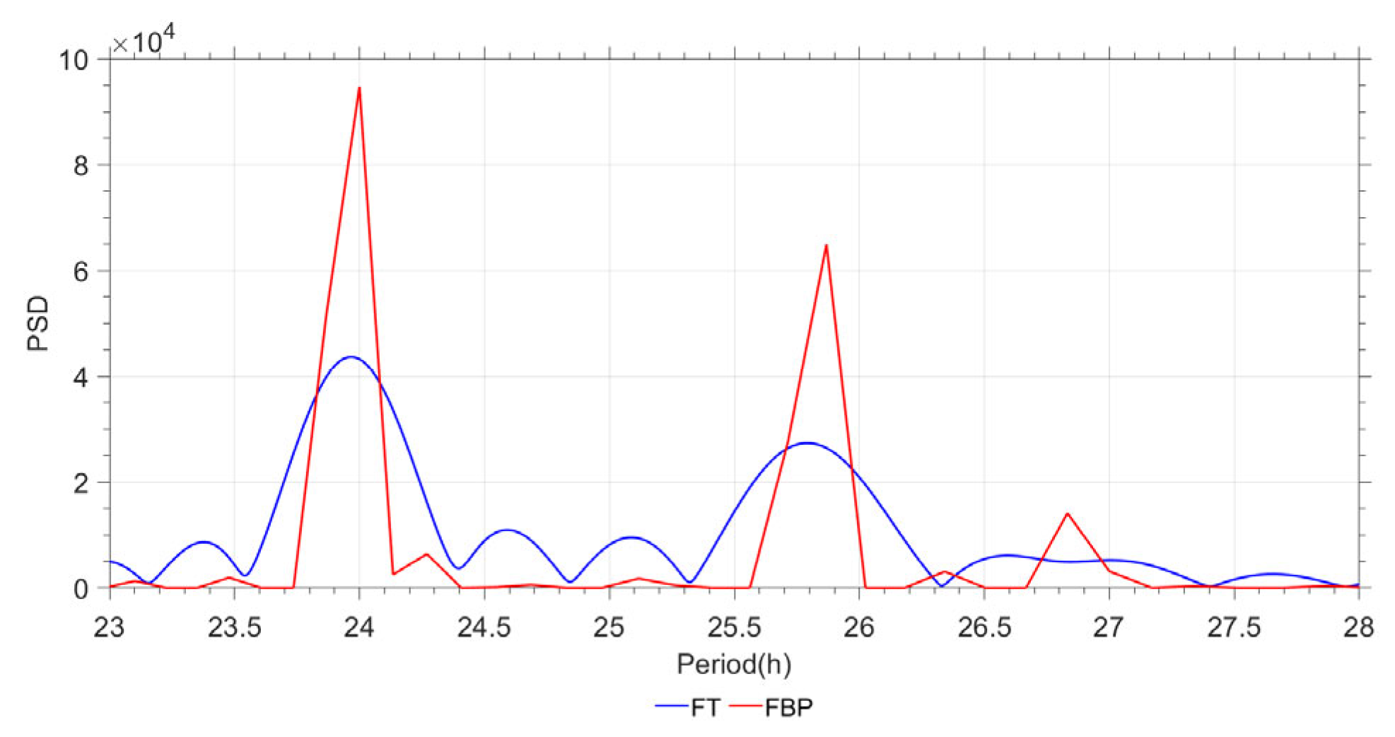
The signal underwent both Fourier spectrum [34] and Fourier Basis Pursuit Band Pass Filter (FBPBPF) [35,36,37,38,39] spectrum analysis, with results shown in Figure 2. Compared to FT, FBPBPF reduced sidelobe interference, concentrating energy more effectively; however, both the FT and FBPBPF methods suffered from mutual interference between closely spaced tidal components due to their short time durations, rendering them ineffective at separating the closely spaced K1 and P1 components. The non-reconstruction NTFT method effectively avoided these issues, achieving superior separation performance within the same duration.

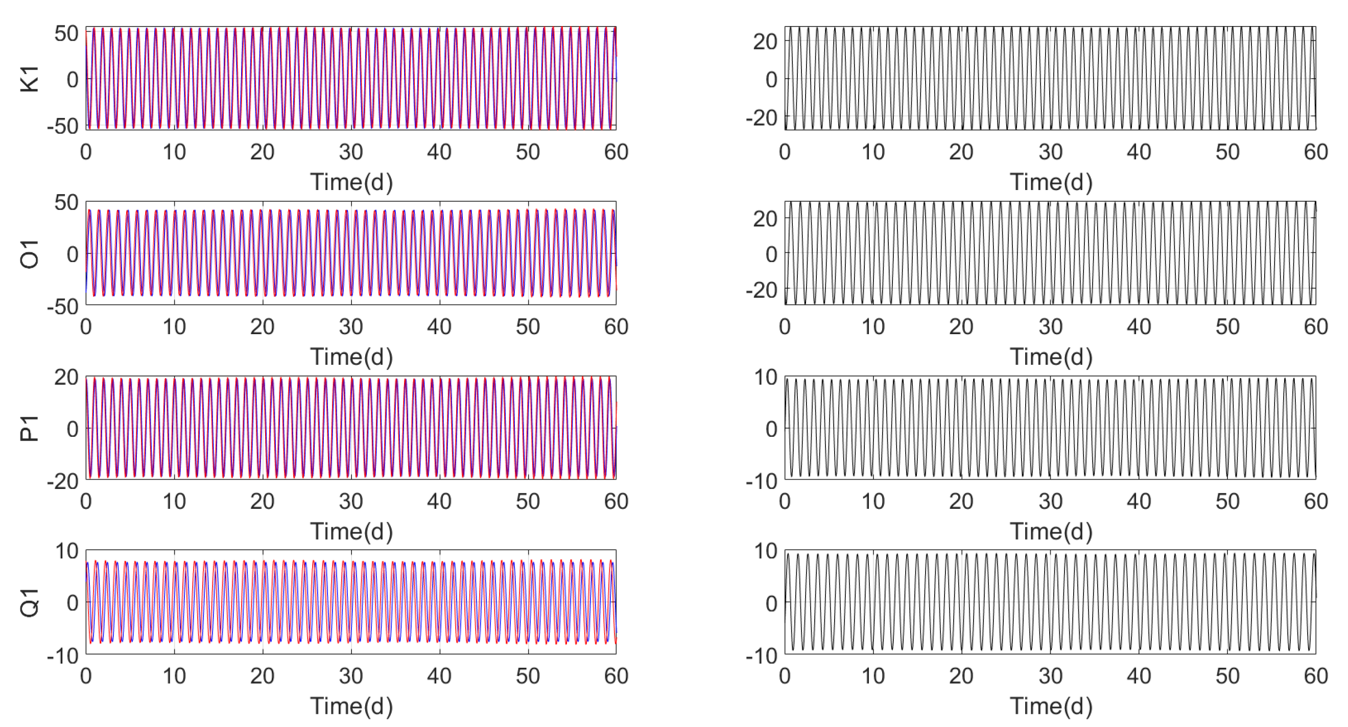
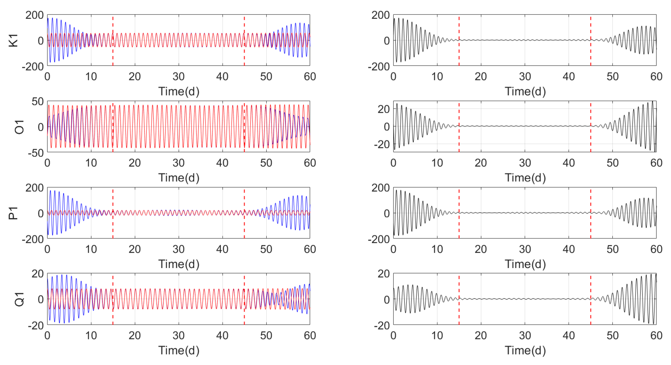
Using traditional harmonic analysis, FBPBPF, and non-reconstruction NTFT methods sequentially, four diurnal tidal waves were separated from the simulated signal (where FBPBPF failed to separate K1 and P1, and was, thus, excluded). As harmonic analysis yields a single signal (Figure 3), it cannot fully describe amplitude variations over time, and the phase delay obtained from short data durations is inaccurate. The FBPBPF method can be used to approximate the actual signal more closely by adjusting the frequency band range during reconstruction; however, the reconstructed result (Figure 4) still exhibits discrepancies with the simulated signal, and the K1 and P1 components cannot be fully separated.

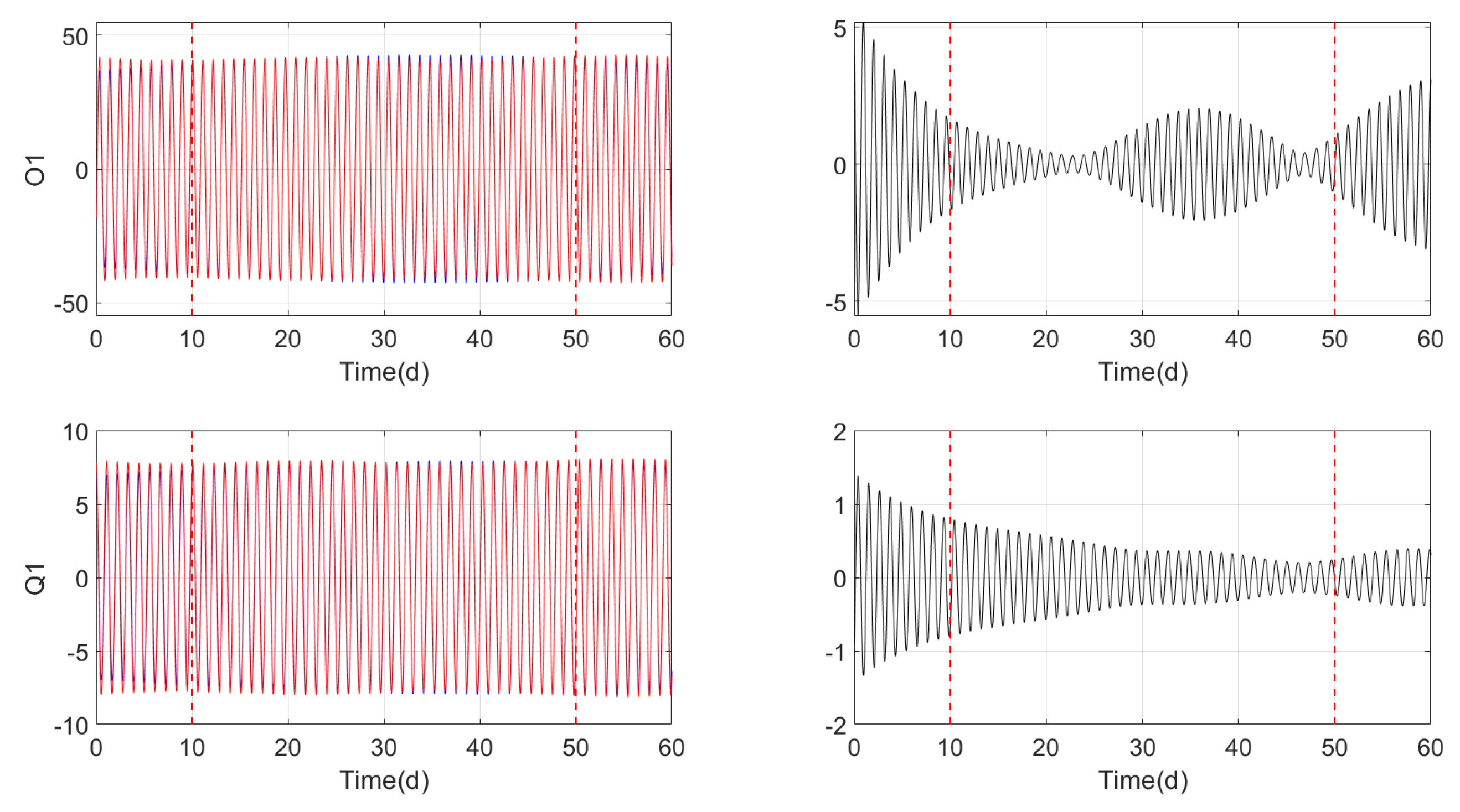
In comparison, the results reached through the non-reconstruction NTFT method (Figure 5) show that, apart from the corresponding edges at both ends, the main bodies of different tidal waves can be perfectly aligned with the theoretical values. When the window width was set to 200 h, the edge effect was approximately 15 days; after excluding the edge effect intervals for all three methods, the simulation values and separation results within the effective intervals were compared, after which the maximum difference, root mean square error, and signal-to-noise ratio were calculated sequentially, as shown in

Table 1. Comparison of separation performance among three methods.

Tidal Wave Separation	Method	Max (%)	RMSE (%)	SNR (dB)
K1	Harmonic Analysis	50.76	35.43	5.99
	FBPBPF	/	/	/
	Non-Reconstruction NTFT	7.61	3.60	25.94
O1	Harmonic Analysis	70.98	49.60	3.07
	FBPBPF	4.95	2.12	30.57
	Non-Reconstruction NTFT	0.86	0.53	42.50
P1	Harmonic Analysis	49.65	34.53	6.02
	FBPBPF	/	/	/
	Non-Reconstruction NTFT	22.25	10.26	17.33
Q1	Harmonic Analysis	118.44	82.57	−1.68
	FBPBPF	9.97	4.17	24.51
	Non-Reconstruction NTFT	5.36	2.82	27.68

. The non-reconstruction NTFT method yielded the best extraction results among the three approaches, with detected periods and amplitudes nearly identical to theoretical values, thus demonstrating NTFT’s capability for signal separation and extraction; hence, for subsequent experiments detailed in this paper, we employed the non-reconstruction NTFT method.

4. Analysis of Pre-Seismic Disturbances in Solid Tidal Amplitude Factors

4.1. Data Preparation

Superconducting gravimeter data were downloaded from the Global Geodynamics Project (GGP) database website (https://isdc.gfz-potsdam.de/igets-data-base/, accessed on 3 March 2025). Level 2 data, which incorporate instrument disturbance corrections for gravity and pressure measurements, are suitable for tidal analysis [40];

Table 2. Basic station information.

Station Name	Abbreviation	Instrument	Latitude	Longitude	Elevation
Bad Homburg	BH_1	CD030_L	50.23° N	8.61° E	190.00 m
	BH_2	CD030_U
Canberra	CB	GWR C031	35.32° S	149.01° E	762.75 m
Membach	MB	GWR C021	50.61° N	6.01° E	250.00 m
Medicina	MC	GWR C023	44.52° N	11.65° E	28.00 m
Metsahovi	ME	GWR T020	60.22° N	24.40° E	55.60 m
Moxa	MO_1	CD034_L	50.64° N	11.62° E	455.00 m
	MO_2	CD034_U
Ny-Alesund	NY	GWR C039	78.93° N	11.87° E	43.00 m
Strasbourg	ST	GWR C026	48.62° N	7.68° E	180.00 m
Sutherland	SU_1	D037_L	32.38° S	20.81° E	1791.00 m
	SU_2	D037_U
TIGO Concepcion	TC	GWR RT038	36.84° S	73.03° W	156.14 m
Vienna	VI	GWR C025	48.25° N	16.36° E	192.44 m
Walferdange	WA	OSG-CT40	49.66° N	6.153° E	295.00 m
Wettzell	WE_2	CD029_U	49.14° N	12.88° E	613.70 m

presents the selected stations and their fundamental details, for which data were sampled at 1 min intervals. All stations possess long-term continuous observation capabilities, with sampling frequency and precision meeting requirements for solid tide signal analysis. According to the Nyquist sampling theorem, a 1 h sampling interval is sufficiently dense for component wave extraction; consequently, the data sequence was downsampled from minute-to-minute to hourly intervals.

4.2. Analysis of Solid Tidal Amplitude Factor Variations

For this study, we examined the pre-seismic solid tidal anomaly of the Sumatra earthquake that occurred at 00:58:55 UTC on 26 December 2004; multiple global seismic monitoring agencies determined the earthquake’s moment magnitude (Mw) to be 9.0 (GCMT: https://www.globalcmt.org/, accessed on 3 March 2025). Tidal wave separation was performed using data from the above 16 stations, covering a period from 2004 to 2005; the analysis window for the data spans from 1 March 2004 to 30 November 2005. Pre-seismic disturbance analysis was conducted using the Q1 component of the tidal waves from these 16 stations.

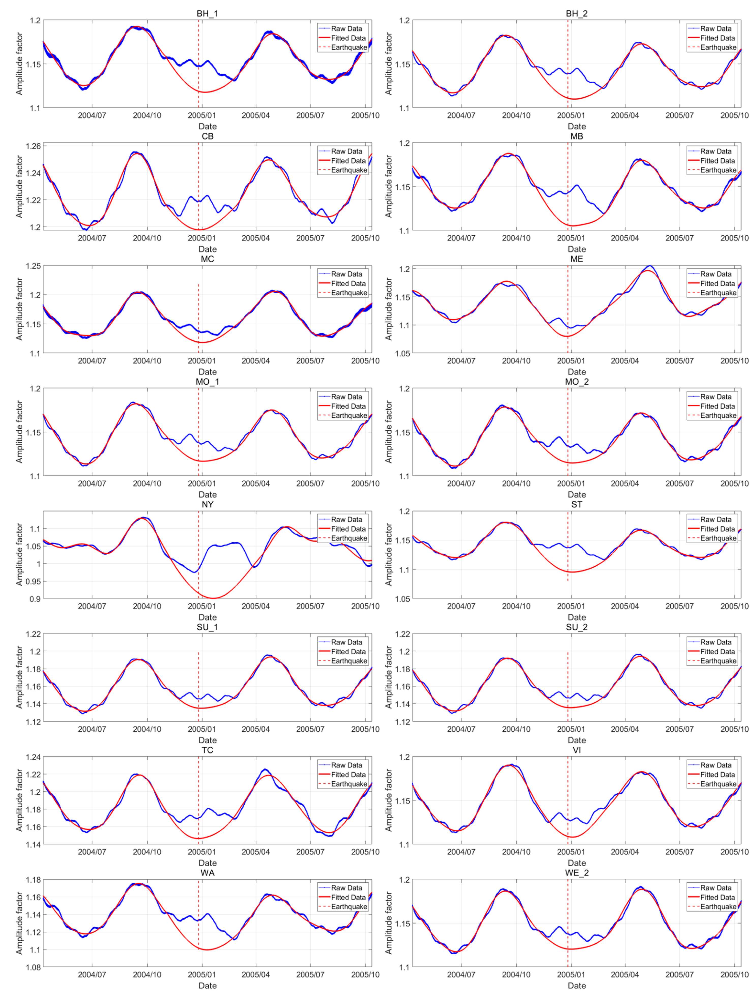
Following instrument disturbance correction of gravity and pressure data from the 16 stations’ superconducting gravimeters, the Q1 tidal component was extracted using the non-reconstruction NTFT method (with a 15-day period at both the start and end excluded from the amplitude factor calculation), yielding the observed Q1 tidal component values. Theoretical Q1 tidal component values were calculated using Equation (14) and the Tamura tidal table. As indicated through Equation (13), the ratio of the measured amplitude to the theoretical amplitude of the Q1 component at each station was employed as the amplitude factor, which enabled the quantitative calculation of the amplitude factor for the Q1 component across all 16 stations (blue line in Figure 6). The results were then fitted, yielding the outcome depicted as the red line in Figure 6, which further corroborates the anomalous variations in amplitude factors observed both before and after the seismic event.

The results in Figure 6 reveal that the amplitude factors for the Q1 tidal component at all 16 stations exhibited distinct anomalous fluctuations during the period preceding the 2004 Sumatra earthquake (red dashed line in Figure 6). Compared to the stable periods before and after the earthquake, the trend of amplitude factor fluctuations changed markedly, gradually returning to normal post-seismic event; furthermore, these anomalous fluctuations demonstrated a degree of synchronisation across different stations.

4.3. Pre-Seismic Disturbance Analysis of Amplitude Factors

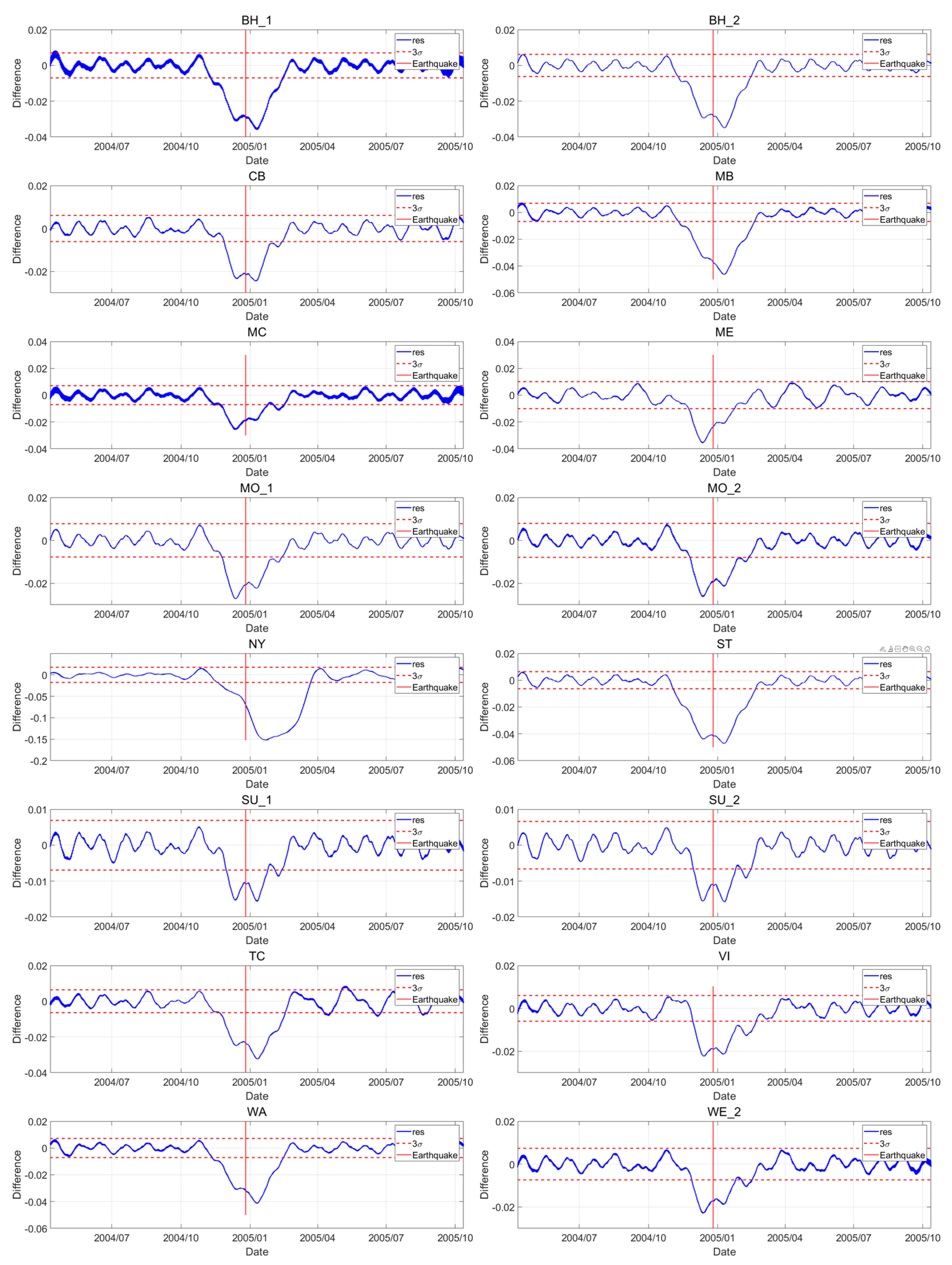
Residuals were calculated using the fitted and observed values from Figure 6. To objectively identify abnormal fluctuations in the amplitude factor of the residuals, we employed the Pauta criterion for outlier detection, which states that the theoretical probability of data values falling within the interval of the mean (μ) ± 3 times the standard deviation (σ) is approximately 99.73%. First, a period without significant disturbances before the earthquake (the 2nd to 3rd months before the earthquake) was selected as the pre-earthquake quiet period, and the standard deviation (σ) of the residuals during this period was calculated; to verify the robustness of the quiet period window selection, the standard deviations of the residuals for the 1st–2nd months and the 3rd–4th months before the earthquake were also calculated (

Table 3. Standard deviation of residuals for different windows.

Station	${\mathit{\sigma }}_{\mathbf{1}\mathbf{-}\mathbf{2}}$	${\mathit{\sigma }}_{\mathbf{2}\mathbf{-}\mathbf{3}}$	${\mathit{\sigma }}_{\mathbf{3}\mathbf{-}\mathbf{4}}$
NY	0.0030	0.0035	0.0038
CB	0.0026	0.0020	0.0024
MB	0.0021	0.0023	0.0023
MC	0.0026	0.0024	0.0025
MO_1	0.0023	0.0019	0.0020
MO_2	0.0022	0.0020	0.0019
ST	0.0024	0.0021	0.0023
WE_2	0.0026	0.0021	0.0022
TC	0.0026	0.0021	0.0026
WA	0.0024	0.0024	0.0023
BH_1	0.0022	0.0023	0.0024
BH_2	0.0021	0.0021	0.0023
SU_1	0.0025	0.0023	0.0022
SU_2	0.0024	0.0022	0.0021
ME	0.0018	0.0033	0.0033
VI	0.0022	0.0020	0.0021
Average	0.0024	0.0023	0.0024

). The results show that the average differences among the three are less than 5% (${\sigma }_{1-2}\approx 0.0024,{\sigma }_{2-3}\approx 0.0023,{\sigma }_{3-4}\approx 0.0024$), indicating that the σ defined based on the 2nd–3rd months before the earthquake has good stability and is not affected by minor adjustments to the window. Subsequently, using σ ± 2σ and ±3σ as thresholds, an anomaly scan was performed over the entire study period, including for both pre- and post-earthquake phases. When the threshold of ±3σ was selected, the probability of values falling within the interval was >99.75%, as shown in

Table 4. Probability of anomalies under different thresholds.

Station	$\pm \mathit{\sigma }$	$\pm 2\mathit{\sigma }$	$\pm 3\mathit{\sigma }$
NY	0.4498	0.0857	0
CB	0.4621	0	0
MB	0.5125	0.1821	0.0167
MC	0.3788	0.0448	0
MO_1	0.5058	0.0750	0
MO_2	0.4812	0.0714	0
ST	0.4712	0.1599	0
WE_2	0.4597	0.0294	0
TC	0.3836	0.0143	0
WA	0.4772	0.1329	0
BH_1	0.4546	0.1142	0.0210
BH_2	0.4712	0.1770	0.0016
SU_1	0.4522	0.0266	0
SU_2	0.4613	0.0194	0
ME	0.3276	0	0
VI	0.4169	0.0099	0
Average	0.4479	0.0714	0.0025

and Figure 7.

The time interval between the last instance of residual amplitude factor exceeding the threshold and the earthquake occurrence was statistically analysed for Q1 tidal waves, as shown in

Table 5. Pre-seismic anomaly timing statistics.

Station	$\pm 3\mathit{\sigma }$	Test Against Population Mean (p-Value)	Probability Estimate P (X ≥ t)	95% Confidence Interval (Days)
NY	38 days	0.42	0.28	[32, 44]
CB	29 days	0.87	0.62	[24, 34]
MB	47 days	0.06	0.12	[40, 54]
MC	33 days	0.65	0.41	[28, 38]
MO_1	32 days	0.71	0.44	[27, 37]
MO_2	31 days	0.76	0.47	[26, 36]
ST	54 days	0.01	0.05	[46, 62]
WE_2	29 days	0.87	0.62	[24, 34]
TC	35 days	0.55	0.35	[30, 40]
WA	45 days	0.09	0.15	[38, 52]
BH_1	47 days	0.06	0.12	[40, 54]
BH_2	47 days	0.06	0.12	[40, 54]
SU_1	26 days	0.92	0.70	[21, 31]
SU_2	27 days	0.89	0.67	[22, 32]
ME	33 days	0.65	0.41	[28, 38]
VI	27 days	0.89	0.67	[22, 32]
Overall	36.3 $\pm$ 9.2	-	-	[33.2, 39.4]

. When using $\pm 3\sigma$ as the threshold, pre-seismic disturbances could be detected as early as 26 days prior. Table 5 displays the observed values and statistical inference results of the anomaly lead time for each station; overall, the average anomaly lead time across the 16 stations was 36.3 days, with a standard deviation of 9.2 days. Except for station ST, the differences between the stations and the population mean were not statistically significant (p > 0.05), indicating that the anomaly lead times for most stations were consistent with the overall average level. Station ST exhibited the longest anomaly lead time (54 days) and showed a significant difference from the population mean (p = 0.01); its probability estimate was only 0.05, which qualifies as a low-probability event. In terms of probability estimates, the P(X ≥ t) values for most stations ranged from 0.12 to 0.70, suggesting that the observed anomaly lead times were relatively common under the assumed distribution. The 95% confidence intervals for each station overlap, further supporting the conclusion that there were no significant differences in anomaly lead times among the stations. The 95% confidence interval for the overall mean was [33.2, 39.4] days, providing a reference range for predicting future anomaly lead times.

The instrument models, geographical locations, and environmental conditions of the above 16 stations vary considerably; this diversity ensures that the anomalous fluctuations in the Q1 tidal wave amplitude factor are not attributable to instrumentation errors or environmental interference. Further quantitative analysis reveals that all 16 stations exhibited changes in the Q1 tidal wave amplitude factor exceeding the threshold range proposed in this paper approximately one month prior to the earthquake, a result which confirms the presence of significant anomalous perturbations in the gravity solid tide preceding the 2004 Sumatra earthquake, providing crucial empirical evidence for studies linking solid tide anomalies to seismic activity.

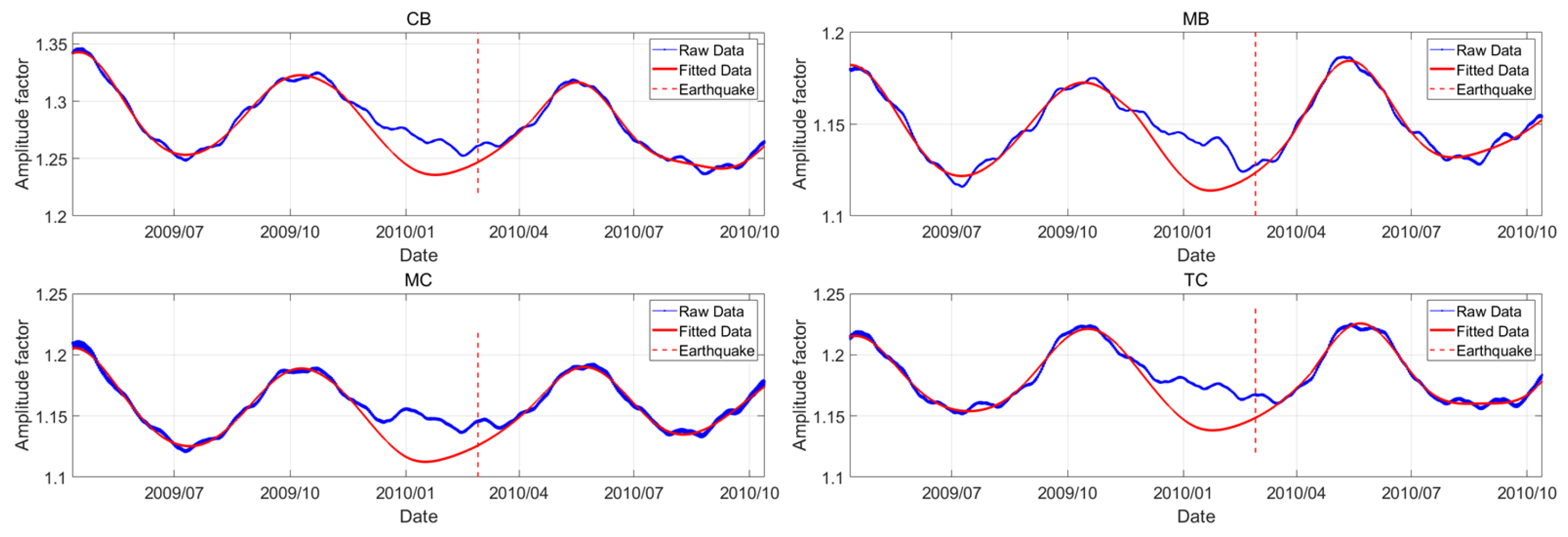
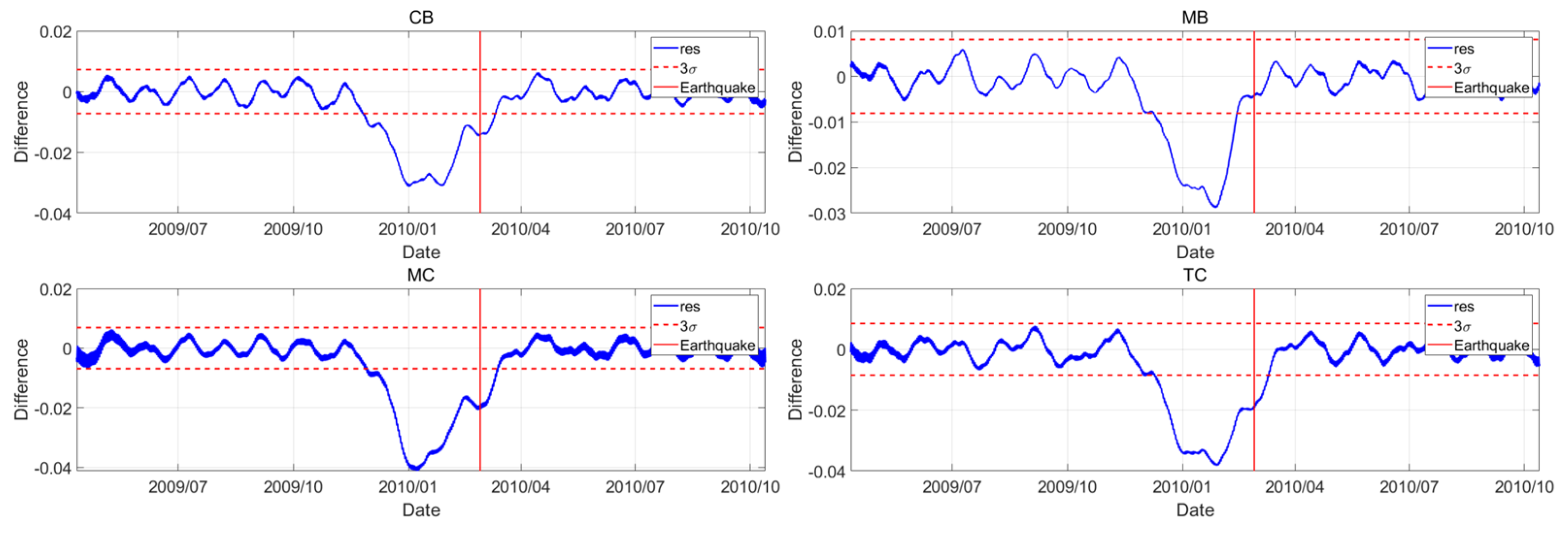
In order to avoid the possibility that the pre-seismic anomalous disturbances in the amplitude factor of the Q1 tidal wave before the 2004 Sumatra earthquake were merely coincidental, we selected 4 (Canberra, Membach, Medicina, and TIGO Concepcion) of the 16 stations provided in Table 2 to validate the findings using the Chilean earthquake that occurred on 27 February 2010, the results of which are shown in Figure 8 and Figure 9. By taking the periods from April to October 2004 in Figure 7, and from April to October 2009 and April to October 2010 in Figure 9 as quiet periods, the two major earthquakes mutually verify that the anomalous disturbances in the amplitude factor of the Q1 tidal wave before these earthquakes exhibit universality, rather than being coincidental phenomena.

5. Conclusions

In this study, we focused on optimising the separation method for gravitational solid tides and conducting dynamic analyses of amplitude factors. Through comparative experiments and data validation, the following conclusions were drawn:

• The non-reconstruction NTFT method employed herein enhances the separation efficiency of primary tidal components, compared to data processing techniques such as harmonic analysis. The proposed method enables precise separation of the four principal gravitational solid tidal components using shorter time series observations, effectively narrowing the data processing time window and substantially improving the timeliness of gravitational solid tidal observations.
• Addressing the limitation of traditional harmonic analysis methods, which yield fixed amplitude factors over a fixed period and fail to reflect the temporal dynamics of tidal factors, the proposed amplitude factor calculation method enhances temporal resolution. Employing the non-reconstruction NTFT method allows us to unbiasedly determine the instantaneous period, amplitude, and phase of the signal, outputting time-varying amplitude factors with higher temporal resolution.
• The presented study constitutes a single-event case study. Through quantitative analysis of data from 16 stations, we confirmed the presence of anomalous disturbances in the amplitude factor of gravity solid Earth tides prior to strong earthquakes. While the correlation revealed is compelling, it requires further testing with other large earthquake events. Additionally, although a statistical anomaly has been detected, we do not propose or test a specific physical model for how crustal stress alters the Q1 tidal amplitude factor.
• The physical mechanism behind the pre-seismic anomalies in the gravity solid Earth tide amplitude factor may involve detectable changes in the physical properties (such as elasticity, inelasticity, porosity, density, and fluid saturation) of the crust in and around the source region during the earthquake preparation process; these changes alter a region’s ability to respond to periodic tidal stresses, a phenomenon which provides a window for utilising continuous, high-precision gravity observations in the study of physical prediction and precursor mechanisms for earthquakes. However, due to the complexity of the mechanism and the demanding observational conditions, transforming the proposed method into a reliable earthquake forecasting tool will require extensive research on physical models, accumulation of case studies, and in-depth interdisciplinary exploration (involving solid Earth physics, hydrogeology, rock mechanics, etc.).

Based on these findings, future research may deepen exploration in the three following directions: Firstly, further mitigating the edge effects of the non-reconstruction NTFT method would enable tidal wave separation using shorter time series data, thereby allowing for analysis of the dynamic patterns of time-varying amplitude factors across different earthquakes. Secondly, studying seismic mechanisms would allow us to deeply analyse the intrinsic relationship between gravitational solid tidal dynamics and major seismic events. Thirdly, given that our current understanding of the correlation between tidal amplitude factor anomalies and earthquakes remains at the phenomenological level, limited to specific case studies, and the underlying physical mechanisms linking “crustal stress accumulation–tidal response anomalies–earthquake triggering” have yet to be fully clarified, there is an urgent need for more systematic research. By integrating and cross-verifying multi-source observational data (such as gravity, geomagnetism, and crustal deformation), we aim to clarify, through future efforts, how to utilise pre-seismic disturbance observations, similar to those obtained in this study, in order to more accurately and reliably determine the future time windows, epicentre locations, and magnitudes of strong earthquakes, which will provide a quantifiable theoretical basis and technical support for short-term and impending earthquake prediction.

References

1. Zhang, L.; Chen, L.; Zhang, J. Variation characteristics of tidal factors before Mongolia MS5.9 earthquake on March 20, 2020. Inland Earthq. 2022, 36, 338–346. (In Chinese) [Google Scholar] [CrossRef]
2. Han, G.; Yu, H.; Zhao, B.; Ma, Y.; Yuan; Li, Z. Application of the Korla volumetric strain to explore the triggering effects of tidal stress on tidal deformation before earthquakes. Geomatics, Nat. Hazards Risk 2024, 15, 2357633. [Google Scholar] [CrossRef]
3. Liu, Y.; Zhang, F.; Zhang, H.; Xie, X.; Li, S. Characteristics of coseismic responses of groundwater level in Jiaji well, China. Geomat. Nat. Hazards Risk 2024, 15, 2331018. [Google Scholar] [CrossRef]
4. Yu, H.; Yan, R.; Deng, S.; Liu, J.; Xue, Y.; Li, G.; Xie, M.; Ma, Y.; Zhang, X.; Ma, Y.; et al. Improved medium-to-short-term earthquake predictions in China in 2022. Geomat. Nat. Hazards Risk 2024, 15, 2350482. [Google Scholar] [CrossRef]
5. Shi, Z.; Wang, G. Relationship between the Earth tidal factor and phase lag of groundwater levels in confined aquifers and the Wenchuan Ms8.0 earthquake of 2008. Sci. China Earth Sci. 2013, 56, 1722–1730. [Google Scholar] [CrossRef]
6. Xia, J.; Dai, Y. An Unsupervised Learning Method for Suppressing Ground Roll in Deep Pre-Stack Seismic Data Based on Wavelet Prior Information for Deep Learning in Seismic Data. Appl. Sci. 2024, 14, 2971. [Google Scholar] [CrossRef]
7. Li, Y.; Chen, L. Analysis of the seismicity related to the tidal stress prior to the Mw7.8 Kahramanmaras, Türkiye earthquake. Geomat. Nat. Hazards Risk 2024, 15, 2284118. [Google Scholar] [CrossRef]
8. Gao, X.; Shu, L.; Ma, Z.; Tian, P.; Pan, L.; Zhang, H.; Yang, S. An Investigation of Pre-Seismic Ionospheric TEC and Acoustic–Gravity Wave Coupling Phenomena Using BDS GEO Measurements: A Case Study of the 2023 Jishishan Ms6.2 Earthquake. Remote Sens. 2025, 17, 2296. [Google Scholar] [CrossRef]
9. Venedikov, A.P.; Arnoso, J.; Vieira, R. VAV: A program for tidal data processing. Comput. Geosci. 2003, 29, 487–502. [Google Scholar] [CrossRef]
10. Wenzel, H.G. Earth tide analysis package Eterna 3.0. Bull. D’information Marees Terr. 1994, 118, 8719–8722. [Google Scholar]
11. Tamura, Y. BAYTAP-G in TIMSAC-84. Comput. Sci. Monogr. 1985, 22, 56–117. [Google Scholar]
12. Camp, M.V.; Vauterin, P. Tsoft: Graphical and interactive software for the analysis of time series and Earth tides. Comput. Geosci 2004, 31, 631–640. [Google Scholar] [CrossRef]
13. Hinderer, J.; Riccardi, U.; Rosat, S.; Boy, J.P.; Hector, B.; Calvo, M.; Littel, F.; Bernard, J.D. A study of the solid earth tides, ocean and atmospheric loadings using an 8-year record (2010–2018) from superconducting gravimeter OSG-060 at Djougou (Benin, West Africa). J. Geodyn. 2020, 134, 101692. [Google Scholar] [CrossRef]
14. Liu, L.; Hsu, H.; Grafarend, E.W. Normal Morlet wavelet transform and its application to the Earth’s polar motion. J. Geophys. Res. 2007, 112, 2006JB004895. [Google Scholar] [CrossRef]
15. Foreman, M.G.G.; Henry, R.F. The harmonic analysis of tidal model time series. Adv. Water. Resour. 1989, 12, 109–120. [Google Scholar] [CrossRef]
16. Baiyang, C.; Fuqiong, H. The influence of time window length selection on tidal factor calculation. Seismol. Geomagn. Obs. Res. 2023, 44, 286–288. (In Chinese) [Google Scholar]
17. Ya, H.; Chongyang, S.; Jin, W.; Guiju, W.; Hongbo, T. Temporal and Spatial Variation of Gravity Tide Parameters before the Lushan M7.0 Earthquake in 2013. J. Geod. Geodyn. 2020, 40, 165–169+197. (In Chinese) [Google Scholar] [CrossRef]
18. Yang, Y.; Wei, X. Gravitational Tides and Seismogenic Anomaly Research in Urumqi. Inland Earthq. 1995, 104–111. (In Chinese) [Google Scholar] [CrossRef]
19. Marchetti, D. Observation of the Preparation Phase Associated with Mw = 7.2 Haiti Earthquake on 14 August 2021 from a Geophysical Data Point of View. Geosciences 2024, 14, 96. [Google Scholar] [CrossRef]
20. Dong, J.; Ke, B.; Yin, L. Sensitivity of GGP superconducting gravimeters in detecting pre-seismic gravity anomalies. Adv. Space. Res. 2025. [Google Scholar] [CrossRef]
21. Chen, J.; Xiong, P.; Wu, H.; Zhang, X.; Zhang, X.; Zhang, T.; Ruan, Q. Pre-seismic anomalies and co-seismic disturbance induced by the 2024 Mw 7.1 Wushi earthquake: Multi-GNSS observations and modeling. Geomat. Nat. Hazards Risk 2024, 15, 2422024. [Google Scholar] [CrossRef]
22. Xianxin, T.; Pinji, L.; Cheng, W.; Yifan, A.; Zhihui, Z.; Hui, W. Variation Characteristics and Influencing Factors of M2 Wave Tidal Factor of Extensometer at Yichang Seismic Station. J. Geod. Geodyn. 2025, 45, 929–936. (In Chinese) [Google Scholar] [CrossRef]
23. Ikhwan, M.; Haditiar, Y.; Wafdan, R.; Ramli, M.; Muchlisin, Z.A.; Rizal, S. M2 tidal energy extraction in the Western Waters of Aceh, Indonesia. Renew. Sust. Energ. Rev. 2022, 159, 112220. [Google Scholar] [CrossRef]
24. Parke, M.E. O1, P1, N2 models of the global ocean tide on an elastic earth plus surface potential and spherical harmonic decompositions for M2, S2, and K1. Mar. Geod. 1982, 6, 35–81. [Google Scholar] [CrossRef]
25. Parke, M.E.; Hendershott, M.C. M2, S2, K1 models of the global ocean tide on an elastic earth. Mar. Geod. 1980, 3, 379–408. [Google Scholar] [CrossRef]
26. Schwiderski, E.W. Atlas of ocean tidal charts and maps, Part I: The semidiurnal principal lunar tide M2. Mar. Geod. 1983, 6, 219–265. [Google Scholar] [CrossRef]
27. Liu, L.; Hsu, H. Time-Frequency Transform: Inversion and Normalization; Hubei Science and Technology Press: Wuhan, China, 2009. [Google Scholar]
28. Liu, L.; Hsu, H. Inversion and normalization of time-frequency transform. In Proceedings of the 2011 International Conference on Multimedia Technology, Hangzhou, China, 26–28 July 2011; IEEE: Hangzhou, China, 2011; pp. 2164–2168. [Google Scholar]
29. Liu, L.; Wang, G.; Su, X.; Sun, X.; Hu, H.; Luo, X. Harmonicity Spectrum. OJS 2023, 13, 761–768. [Google Scholar] [CrossRef]
30. Cai, S.; Liu, L.; Wang, G. Short-term tidal level prediction using normal time-frequency transform. Ocean Eng. 2018, 156, 489–499. [Google Scholar] [CrossRef]
31. Su, X. Standard Time-Frequency Transform Theory and Its Geoscience Application; University of Chinese Academy of Sciences: Beijing, China, 2014. (In Chinese) [Google Scholar]
32. Tamura, Y. A harmonic development of the tide-generating potential. Bull. D’information Marees Terr. 1987, 99, 6813–6855. [Google Scholar]
33. Tamura, H.; Collins, C.O., III. Progress of ocean wave measurement. Coast. Eng. J. 2024, 66, 1–2. [Google Scholar] [CrossRef]
34. Fourier, J. Théorie de la Propagation de la Chaleur dans les Solides; Institute of France: Paris, France, 1807. [Google Scholar]
35. Wang, G.; Liu, L.; Su, X.; Liang, X.; Yan, H.; Tu, Y.; Li, Z.; Li, W. Variable Chandler and Annual Wobbles in Earth’s Polar Motion During 1900–2015. Surv. Geophys. 2016, 37, 1075–1093. [Google Scholar] [CrossRef]
36. Olshausen, B.A.; Sallee, P.; Lewicki, M.S. Learning Sparse Image Codes using a Wavelet Pyramid Architecture. In Advances in Neural Information Processing Systems 13: Proceedings of the 2000 Conference: Fourtheenth Annual Neural Information Processing Systems (NIPS) Conference; Curran Associates Inc.: Red Hook, NY, USA, 2000. [Google Scholar]
37. Starck, J.L.; Elad, M.; Donoho, D.L. Image decomposition via the combination of sparse representations and a variational approach. IEEE Trans. Image. Process. 2005, 14, 1570–1582. [Google Scholar] [CrossRef]
38. Li, Y.; Cichocki, A.; Amari, S. Analysis of Sparse Representation and Blind Source Separation. Neural. Comput. 2004, 16, 1193–1234. [Google Scholar] [CrossRef]
39. Elad, M.; Aharon, M. Image Denoising Via Learned Dictionaries and Sparse representation. In Proceedings of the 2006 IEEE Computer Society Conference on Computer Vision and Pattern Recognition (CVPR’06), 17–22 June 2006; IEEE: New York, NY, USA, 2006; pp. 895–900. [Google Scholar]
40. Boy, J.P.; Rosat, S.; Hinderer, J.; Littel, F. Superconducting Gravimeter Data from Strasbourg-Level 1. GFZ Data Serv. 2017. [Google Scholar] [CrossRef]
Figure 1. Simulated signal.
Geosciences 16 00053 g001
Figure 2. Fourier spectrum and FBPBPF spectrum.
Geosciences 16 00053 g002
Figure 3. Harmonic analysis method (blue line: harmonic analysis-separated signal; red line: simulated signal; black line: difference).
Geosciences 16 00053 g003
Figure 4. FBPBPF method (blue line: FBPBPF-separated signal; red line: simulated signal; black line: difference; area outside red dashed line: edge effect influence zone).
Geosciences 16 00053 g004
Figure 5. Non-reconstruction NTFT method (blue line: NTFT-separated signal; red line: simulated signal; black line: difference; region outside red dashed line: edge effect influence zone).
Geosciences 16 00053 g005
Figure 6. Amplitude factors for Q1 tidal waves at 16 stations (regarding the 2004 Sumatra earthquake).
Geosciences 16 00053 g006
Figure 7. Amplitude factor residuals for Q1 tidal waves at 16 stations (regarding the 2004 Sumatra earthquake).
Geosciences 16 00053 g007
Figure 8. Amplitude factors for Q1 tidal waves at 4 stations (regarding the 2010 Chile earthquake).
Geosciences 16 00053 g008
Figure 9. Amplitude factor residuals for Q1 tidal waves at 4 stations (regarding the 2010 Chile earthquake).
Geosciences 16 00053 g009