Fault-Tolerant Control of Switched Nonlinear Systems Under State Constraints and Multiple Time-Varying Faults

Abstract

This paper proposes an adaptive fault-tolerant control strategy for nonlinear switched systems subject to state constraints and time-varying faults. Within a backstepping framework, multiple Lyapunov integral barrier functions are constructed to enforce state constraints, while radial basis function neural networks and adaptive laws compensate for actuator and sensor faults. Under average dwell time switching, the closed-loop system is rigorously proven to achieve fast practical finite-time stability and excellent output tracking performance, ensuring all signals remain bounded without violating constraints. The approach is validated via a variable-load nonlinear spring–damper simulation.

1. Introduction

A switched system consists of a sequence of continuous-time or discrete-time subsystems and a switching rule governing their transitions. Unlike conventional non-switched systems, switched systems exhibit complex dynamical behaviors: even asymptotically stable subsystems may lead to divergent closed-loop systems under improper switching signals, while unstable subsystems can be stabilized via well-designed switching logic. Control and stability analysis of nonlinear switched systems remain a cutting-edge research topic [1,2,3], which spawned the theory of multiple Lyapunov functions (MLFs). Reference [4] first systematically established the MLF framework, proposing that each subsystem can have its own Lyapunov function instead of a globally unified energy function. Reference [5] explored the intrinsic MLF-switched system relationship, transforming multiple Lyapunov stability criteria into a single Lyapunov function via linguistic theory and symbolic dynamics to derive novel stability conditions. Reference [6] addressed input–output-to-state stability of time-varying nonlinear switched systems, extending MLFs to indefinite forms to relax the strict negative definiteness requirement on Lyapunov function derivatives.

Practical switching behaviors are constrained by hardware and energy limitations. Time constraints, particularly dwell time and average dwell time (ADT), are widely adopted for their engineering feasibility. ADT allows occasional high-frequency switching while regulating the overall average switching frequency, ensuring exponential stability for all-stable-subsystem switched systems when exceeding a threshold [7]. Reference [8] studied linear switched systems with both stable and unstable subsystems, constructing piecewise Lyapunov functions and extending results to systems with nonlinear norm-bounded perturbations. It proved that small perturbations can be compensated via modified switching laws and sufficiently large ADT for exponential convergence. Reference [9] combined ADT with backstepping to propose an adaptive radial basis function (RBF) neural network output feedback controller for uncertain nonlinear switched systems with unmeasurable states, designing independent switching filters and update laws to ensure bounded signals and convergent tracking errors. Reference [10] applied ADT to discrete-time switched systems, deriving necessary and sufficient exponential stability criteria for time-delay systems via higher-order homogeneous switched Lyapunov methods. Reference [11] addressed robust stability of asynchronous time-delay switched systems with ADT, obtaining two sets of sufficient conditions via integral inequalities.

Recent advances in switched systems have also addressed critical challenges in secure control and transient performance optimization. Reference [12] developed an adaptive fuzzy tracking control scheme for switched nonlinear systems subject to false data injection attacks and input saturation, achieving flexible transient performance via a prescribed performance function framework. Reference [13] proposed a sub-domain-awareness adaptive probabilistic event-triggered policy for attack-compensated output control of Markov jump cyber–physical systems, where dynamically matching modes are handled through a novel mode-dependent triggering mechanism. For fault-tolerant control of switched linear parameter-varying systems, reference [14] introduced a bumpless transfer approach that minimizes control signal jumps during mode transitions while maintaining stability. These works highlight the growing research interest in integrating switching control with fault tolerance, security, and transient performance guarantees, which motivates the present study to further address simultaneous actuator and sensor faults under state constraints.

Barrier Lyapunov Functions (BLFs) tend to infinity as system states approach predefined constraint boundaries while remaining positive definite and continuous within the feasible region. References [15,16] used backstepping and logarithmic BLFs to solve output tracking problems for state-constrained nonlinear systems, achieving constraint-free asymptotic tracking under feasible initial conditions and control parameters. References [17,18,19,20] combined logarithmic BLFs with neural networks or fuzzy logic systems to handle unknown functions, designing observers and controllers for systems with unmeasurable states or input delays while enforcing state constraints. Integral Barrier Lyapunov Functions (IBLFs) have also been widely applied to state-constrained nonlinear systems [21,22,23,24]. Reference [25] proposed an adaptive finite-time controller for strict-feedback nonlinear systems with parametric uncertainties and full-state constraints using a novel tangent-type BLF, constructing new tuning functions to eliminate uncertainties and ensure finite-time tracking error convergence without constraint violations.

Beyond traditional control frameworks, recent research has also explored secure and adaptive control strategies for complex nonlinear systems. Reference [26] investigated adaptive neural self-triggered secure control for nonlinear networked PDE-ODE systems subject to unknown deception attacks, where a self-triggered communication mechanism reduces the network transmission burden while maintaining closed-loop stability. Stability analysis has also been extended to optimization and cooperative control frameworks. Reference [27] established global asymptotic stability conditions for autonomous optimization systems, providing a unified Lyapunov-based stability criterion that is applicable to a broad class of dynamical systems. Furthermore, reference [28] addressed the gradient-free cooperative source-seeking problem of quadrotor systems under disturbances and communication constraints, demonstrating the applicability of Lyapunov-based analysis to multi-agent systems with limited communication. These results provide important insights into the stability analysis and adaptive compensation techniques that are relevant to the FTC design for switched nonlinear systems.

Fault-tolerant control (FTC) enables systems to maintain stable operation and acceptable performance under actuator, sensor, or structural faults, enhancing safety and reliability to prevent catastrophic accidents. Reference [29] proposed a fuzzy adaptive compensation scheme for time-varying nonaffine faults. For sensor faults, reference [30] developed a switching-type observer to improve transient performance under unknown faults, while reference [31] designed a fault-compensated state observer for partial sensor failures using cubic absolute-value Lyapunov functions. Reference [32] further addressed multiple sensor faults that invalidate conventional feedback, eliminating their adverse effects. For simultaneous actuator and sensor faults, reference [33] presented an adaptive neural network FTC controller, compensating for multiple fault types (e.g., bias, drift) with reduced computational burden via a single-parameter update mechanism.

This paper focuses on uncertain nonlinear switched systems and investigates in depth the problem of adaptive safe fault-tolerant control under the coexistence of state constraints and simultaneous multiple hardware faults. By integrating RBF neural networks, the backstepping technique, BLFs, and the ADT method, this paper proposes a series of novel adaptive fault-tolerant control schemes. The stability of the closed-loop system is rigorously proved through mathematical analysis, and comprehensive simulation verification is conducted based on a variable-load spring–damper system model. The main contributions of this paper are as follows:

(1)

By employing the ADT method and the MLF approach, local BLFs are constructed for each subsystem rather than a common BLF within the recursive backstepping design framework, which significantly reduces the conservatism of the system design.

(2)

Furthermore, considering severe sensor distortion and high-frequency oscillation, as well as actuator efficiency degradation with fluctuating performance across different subsystem modes, an adaptive safe control strategy is developed that can simultaneously compensate for multiple time-varying hardware faults.

(3)

Rigorous theoretical analysis demonstrates that under the ADT constraint, even when the system is subjected to abrupt multiple faults, the system state variables never violate the state safety constraints. The closed-loop system achieves fast practical finite-time stability and excellent tracking performance, and all signals within the system remain uniformly ultimately bounded.

To further clarify the novelty of this work, we highlight the following distinctive features:

(1)

Unlike traditional IBLF-based methods that impose indirect constraints on tracking errors, our MLIBF enforces direct constraints on faulty states $x_i^F$, thereby preserving the full feasible region and reducing conservatism. This eliminates the restrictive requirement for prior knowledge of virtual control bounds, which is often unattainable in practical applications.

(2)

Unlike most existing FTC schemes that address either actuator faults or sensor faults separately, our method simultaneously handles both types of time-varying faults under the ADT framework. The deep coupling between switching dynamics and multiple simultaneous faults is rigorously addressed through the coordinated design of MLIBF and adaptive compensation laws.

(3)

The piecewise function ${\mathrm{\Theta }}_i$ is innovatively constructed to circumvent the singularity problem inherent in finite-time backstepping, ensuring boundedness of all closed-loop signals while preserving the finite-time convergence property.

(4)

The rigorous finite-time stability analysis under strict state safety constraints and multiple simultaneous faults provides, to the best of our knowledge, a new result for nonlinear switched systems.

Based on the above analysis, distinct features are summarized to explicitly contrast our approach with existing literature in the following Table 1.

Table 1. Distinct features.

References	Fault Type	Switching Handling	Finite-Time
[21]	None	None	No
[22]	Actuator Only	None	No
[31]	Sensor Only	None	No
[33]	Actuator + Sensor	None	No
Our Work	Actuator + Sensor	ADT + MLF	Yes

The rest of this paper is organized as follows. Section 2 presents the system description and problem formulation. Section 3 develops the multiple Lyapunov integral barrier function (MLIBF)-based adaptive fault-tolerant controller design. Section 4 provides the stability analysis under the ADT framework. The simulation results are given in Section 5. Section 6 concludes this paper.

2. System Description and Problem Formulation

Consider the following nonlinear switched systems subject to both sensor and actuator faults,

$$\begin{array}{cc}\hfill {\dot{x}}_i& = g_{i,\sigma \left(t\right)}\left({\overline{x}}_i\right)x_{i+1}+h_{i,\sigma \left(t\right)}\left({\overline{x}}_i\right)+{\phi }_{i,\sigma \left(t\right)}(x,t),i=1,\dots ,n-1\hfill \\ \hfill {\dot{x}}_n& = g_{n,\sigma \left(t\right)}\left({\overline{x}}_i\right)u_{\sigma }+h_{n,\sigma \left(t\right)}\left({\overline{x}}_n\right)+{\phi }_{n,\sigma \left(t\right)}(x,t)\hfill \\ \hfill y& = x_1\hfill \end{array}$$

(1)

where ${\overline{x}}_i={[x_1,\dots ,x_i]}^T\in {\mathbb{R}}^i$ ($i=1,2,\dots ,n$) represents the system state vector; $y\in \mathbb{R}$ is the system output; $\sigma \left(t\right)=k\in {\mathbb{N}}^{+}$ denotes the switching signal, and the system operates in the k-th mode during the time interval $t\in [t_k,t_{k+1})$; $h_{i,k}\left({\overline{x}}_i\right)$ and $g_{i,k}\left({\overline{x}}_i\right)$ represent the unknown smooth nonlinear functions within the system, and there exist two unknown positive constants $\underline{g}$ and $\overline{g}$ such that $\underline{g}<g_{i,k}\left({\overline{x}}_i\right)<\overline{g}$; ${\phi }_{i,k}(x,t)$ denotes the unknown external disturbance; and $u_k$ is the control input of the k-th subsystem, which is subject to the risk of actuator faults.

Based on [29], the following sensor and actuator faults are considered:

$$x_i^F={\beta }_{i,\sigma \left(t\right)}\left(t\right)x_i,i=1,\dots ,n$$

(2)

$$u_k\left(t\right)={\beta }_{0,\sigma \left(t\right)}\left(t\right)v_k$$

(3)

where ${\beta }_{i,\sigma \left(t\right)}\left(t\right)$ and ${\beta }_{0,\sigma \left(t\right)}\left(t\right)$ denote the switched time-varying sensor and actuator fault factors, respectively. These factors are unknown functions, and there exists a positive constant ${\underline{\beta }}_{i,k}$ such that ${\underline{\beta }}_{i,k}<{\beta }_{i,k}\left(t\right)<1$. $v_k$ represents the actual control input. The fault models considered in this paper address the loss-of-effectiveness faults in sensors and actuators under the condition that the fault factors are unknown time-varying functions.

The fault models considered in this paper focus on multiplicative (loss-of-effectiveness) faults in both sensors and actuators. This class of faults is particularly challenging as it directly multiplies the state measurements and control signals, thereby altering the system structure and constraint conditions. It is worth noting that additive bias and drift faults can also be accommodated within the proposed framework by incorporating additional adaptive compensation terms. However, such extensions would increase the computational burden and complexity of the stability analysis. The current method is therefore primarily applicable to systems subject to multiplicative faults, which are common in practical scenarios such as sensor calibration degradation and actuator efficiency loss.

Furthermore, the state safety constraints imply that, even in the presence of sensor faults, the state of each subsystem must satisfy

$$|x_i^F| <M_{c_i},M_{c_i}>0$$

(4)

where the positive constants $M_{c_i}$ define the allowable safety bounds for the faulty measurable states, referred to as the state safety constraints throughout this paper.

In practice, state measurements are obtained through sensors. When sensors experience faults (e.g., loss of effectiveness, drift), the measured values $x_i^F$ no longer equal the true physical states $x_i$. However, control decisions must be made based on these faulty measurements. Therefore, imposing constraints on $x_i^F$ means ensuring that the measured/readable values remain within safe bounds, which is the only information available to the controller. Meanwhile, since the fault factor ${\beta }_{i,k}\left(t\right)$ satisfies ${\underline{\beta }}_{i,k}<{\beta }_{i,k}\left(t\right)<1$, the actual physical state satisfies $|x_i| = |x_i^F|/{\beta }_{i,k}\left(t\right)>|x_i^F|$, meaning that the true state may exceed the measured value. Thus, constraining $x_i^F$ with tighter bounds (i.e., selecting smaller $M_{c_i}$) provides a conservative safety guarantee for the actual physical state.

Remark 1.

The faults described by (2) and (3) are deeply coupled with the switching behaviors. Such complex faults directly induce a fundamental alteration in the system constraints. Owing to the unknown time-varying actuator and sensor fault factors, ${\beta }_{0,\sigma \left(t\right)}$ and ${\beta }_{i,\sigma \left(t\right)}\left(t\right)$, the conventional true state constraints are transformed into the more stringent faulty state constraints (4), which necessitates the innovative construction of the subsequent MLIBF to tackle the constraint challenges.

The objective of this paper is to design a singularity-free adaptive finite-time fault-tolerant controller and an ADT switching law for the nonlinear switched system (1) subjected to multiple faults and state constraints (4). This ensures that the system output can effectively track the reference signal within a finite time, all signals in the closed-loop system remain bounded, and the full-order states strictly satisfy the safety constraints.

Assumption 1.

For all $t>0$, there exist positive constants ${\pi }_0$ and ${\pi }_i$ ($i=1,2,\dots ,n$) such that the reference signal $y_r\left(t\right)$ and its derivatives satisfy

$$|y_r\left(t\right)|\le {\pi }_0\le M_{c_1},|y_r^{\left(i\right)}\left(t\right)|\le {\pi }_i$$

(5)

• Universal Approximation Property of RBF Neural Networks: Radial basis function neural networks are employed in this paper to approximate unknown continuous functions. It is well established that RBF neural networks possess the universal approximation property; i.e., for any continuous function $f\left(X\right)$ defined on a compact set $\mathrm{\Omega }\subset {\mathbb{R}}^q$ and any given accuracy $\epsilon >0$, there exists an RBF neural network with sufficiently many nodes such that

  $$\underset{X\in \mathrm{\Omega }}{sup}\left|f\left(X\right)-W^{*T}S\left(X\right)\right|\le \epsilon$$

  (6)

  where $W^{*}\in {\mathbb{R}}^p$ is the ideal weight vector and $S\left(X\right)\in {\mathbb{R}}^p$ is the basis function vector. This property guarantees that the unknown nonlinear functions ${\overline{f}}_{i,k}\left(X_i\right)$ defined in the subsequent controller design can be approximated with arbitrary accuracy over the compact set of interest.

Lemma 1

([17]). Consider the IBLF $V_i$, which satisfies the following conditions:

$$V(z,\alpha )={\displaystyle \sum _{i=1}^n}{V}_i(z_i,{\alpha }_{i-1})$$

(7)

$$V_i(z_i,{\alpha }_{i-1})={\int }_0^{z_i}{\displaystyle \frac{\sigma k_{c_i}^2}{k_{c_i}^2-{(\sigma +{\alpha }_{i-1})}^2}}d\sigma ,i=1,\dots ,n$$

(8)

$${\displaystyle \frac{z_i^2}{2}}\le V_i\le {\displaystyle \frac{k_{c_i}^2{z}_i^2}{k_{c_i}^2-x_i^2}}$$

(9)

where $|x_i| <k_{c_i}$, and $z_i=x_i-{\alpha }_{i-1}$ (with ${\alpha }_0=y_d$) denotes the tracking error.

Lemma 2.

Consider the differential inequality

$$\dot{V}\le -aV-b{V}^{\rho }+c$$

where $V\ge 0$, $a>0$, $b>0$, $0<\rho <1$, and $c>0$. Then, $V\left(t\right)$ converges to a bounded region in finite time, and the convergence time satisfies

$$T_r\le max\left\{t_0+{\displaystyle \frac{1}{\mathsf{\ell }b(1-\rho )}}ln{\displaystyle \frac{\mathsf{\ell }b{V}^{1-\rho }\left(t_0\right)+a}{a}},t_0+{\displaystyle \frac{1}{b(1-\rho )}}ln{\displaystyle \frac{b{V}^{1-\rho }\left(t_0\right)+\mathsf{\ell }a}{\mathsf{\ell }a}}\right\}$$

for any $0<\mathsf{\ell }<1$.

3. MLIBF-Based Fault-Tolerant Controller Design

In this section, a singularity-free finite-time adaptive FTC strategy is developed for nonlinear switched systems subject to multiple time-varying faults, external disturbances, and state constraints. By leveraging the MLIBF, it is strictly guaranteed that the full-state vectors remain within the predefined safety boundaries under both ADT switching and abrupt multiple faults. Furthermore, a piecewise function is innovatively introduced to circumvent the singularity problem inherent in traditional finite-time backstepping during the differentiation process, ensuring the boundedness of all closed-loop signals. Finally, RBF neural networks and adaptive laws are utilized to compensate for unknown sensor and actuator failure factors. This approach effectively reduces the conservatism of the control design while ensuring the safe, stable, and reliable operation of the constrained system under complex working conditions. Based on the aforementioned theory, the specific recursive backstepping design procedure is detailed as follows:

Step 1: First, the following coordinate transformation is introduced for system (1):

$$\begin{array}{cc}\hfill {\vartheta }_1& = x_1^F-y_r\hfill \\ \hfill {\vartheta }_i& = x_i^F-{\alpha }_{i-1}-y_r^{(i-1)}\hfill \end{array}$$

(10)

where ${\alpha }_{i-1}$ denotes the virtual controller, whose specific expression will be presented in subsequent sections.

Differentiating the tracking error ${\vartheta }_1$ yields

$$\begin{array}{cc}\hfill {\dot{\vartheta }}_1& = {\dot{x}}_1^F-{\dot{y}}_r\hfill \\ \hfill & = {\beta }_{1,k}\left(t\right){\dot{x}}_1+{\dot{\beta }}_{1,k}\left(t\right)x_1-{\dot{y}}_r\hfill \\ \hfill & = {\beta }_{1,k}\left(t\right)\left(g_{1,k}\left(x_1\right)x_2+h_{1,k}\left(x_1\right)+{\phi }_{1,k}\left(x_1\right)\right)+{\dot{\beta }}_{1,k}\left(t\right)x_1-{\dot{y}}_r\hfill \\ \hfill & = {\displaystyle \frac{{\beta }_{1,k}\left(t\right)g_{1,k}\left(x_1\right)}{{\beta }_{2,k}\left(t\right)}}\left({\vartheta }_2+{\alpha }_1+{\dot{y}}_d\right)+{\beta }_{1,k}\left(t\right)h_{1,k}\left(x_1\right)+{\beta }_{1,k}\left(t\right){\phi }_{1,k}\left(x_1\right)\hfill \\ \hfill & + {\dot{\beta }}_{1,k}\left(t\right)x_1-{\dot{y}}_r\hfill \end{array}$$

(11)

Subsequently, IBLF is constructed as follows:

$$V_1^{\vartheta }={\int }_0^{{\vartheta }_1}{\displaystyle \frac{\lambda M_{c_1}^2}{M_{c_1}^2-{(\lambda +y_r)}^2}}d\lambda$$

(12)

The time derivative of $V_1^{\vartheta }$ is given by

$${\dot{V}}_1^{\vartheta }={\displaystyle \frac{{\vartheta }_1{M}_{c_1}^2}{M_{c_1}^2-{\left(x_1^F\right)}^2}}{\dot{\vartheta }}_1+{\dot{y}}_r{\int }_0^{{\vartheta }_1}{\displaystyle \frac{\partial }{\partial y_r}}{\displaystyle \frac{\lambda M_{c_1}^2}{M_{c_1}^2-{(\lambda +y_r)}^2}}d\lambda$$

where

$${\int }_0^{{\vartheta }_1}{\displaystyle \frac{\partial }{\partial y_r}}{\displaystyle \frac{\lambda M_{c_1}^2}{M_{c_1}^2-{\left(\lambda +y_r\right)}^2}}d\lambda =\left({\vartheta }_1{m}_1-{\vartheta }_1{\varrho }_1({\vartheta }_1,y_r)\right),m_1={\displaystyle \frac{M_{c_1}^2}{M_{c_1}^2-{\left(x_1^F\right)}^2}}$$

(13)

$${\varrho }_1({\vartheta }_1,y_r)={\int }_0^1{\displaystyle \frac{M_{c_1}^2}{M_{c_1}^2-{\left(\mu {\vartheta }_1+y_r\right)}^2}}d\mu ={\displaystyle \frac{M_{c_1}}{2{\vartheta }_1}}ln{\displaystyle \frac{\left(M_{c_1}+{\vartheta }_1+y_r\right)\left(M_{c_1}-y_r\right)}{\left(M_{c_1}-{\vartheta }_1-y_r\right)\left(M_{c_1}+y_r\right)}}$$

(14)

By applying L’Hôpital’s rule, we obtain ${lim}_{{\vartheta }_1\to 0}{\varrho }_1({\vartheta }_1,y_r)=M_{c_1}^2/\left(M_{c_1}^2-y_r^2\right)$. Combined with Assumption 1, $y_r$ is bounded and satisfies $\left|y_r\left(t\right)\right|\le {\pi }_0\le M_{c_1}$. Therefore, even when ${\vartheta }_1=0$, ${\varrho }_1({\vartheta }_1,y_r)$ remains bounded in the neighborhood of ${\vartheta }_1=0$. The same boundedness property holds for all subsequent steps.

Remark 2.

Unlike traditional logarithmic BLF that impose indirect state constraints by limiting tracking errors, the IBLF constructed in this paper enforces direct constraints on the actual faulty state $x_1^F$. Based on the error definition ${\vartheta }_i=x_i^F-{\alpha }_{i-1}-y_r^{(i-1)}$ adopted in this work, indirect constraint approaches require prior knowledge of the bounds of the virtual control law ${\alpha }_{i-1}$, which leads to a severe contraction of the initial feasible solution set. The introduction of the IBLF eliminates complex error transformation conditions and preserves the complete original constraint set, thereby significantly reducing the conservatism of the constrained fault-tolerant controller design.

The following MLIBF is constructed:

$$V_{1,k}={\int }_0^{{\vartheta }_1}{\displaystyle \frac{\lambda M_{c_1}^2}{M_{c_1}^2-{\left(\lambda +y_d\right)}^2}}d\lambda +{\displaystyle \frac{{\beta }_{1,k}}{2{\gamma }_1}}{\tilde{\theta }}_1^2$$

(15)

where ${\gamma }_1>0$ is a positive design parameter, and the estimation error of ${\theta }_1$ is defined as ${\tilde{\theta }}_1={\theta }_1-{\widehat{\theta }}_1$.

Combining (12)–(14), the time derivative of $V_{1,k}$ along the trajectory of ${\dot{\vartheta }}_1$ is given by

$$\begin{array}{cc}\hfill {\dot{V}}_{1,k}& = m_1[{\displaystyle \frac{{\beta }_{1,k}\left(t\right)g_{1,k}\left(x_1\right)}{{\beta }_{2,k}\left(t\right)}}\left({\vartheta }_2+{\alpha }_1+{\dot{y}}_r\right)+{\beta }_{1,k}\left(t\right)h_{1,k}\left(x_1\right)\hfill \\ \hfill & +{\beta }_{1,k}\left(t\right){\phi }_{1,k}\left(x_1\right)+{\dot{\beta }}_{1,k}\left(t\right)x_1-{\dot{y}}_r]-{\displaystyle \frac{{\beta }_{1,k}}{{\gamma }_1}}{\tilde{\theta }}_1{\dot{\widehat{\theta }}}_1+m_1{\dot{y}}_r\hfill \\ \hfill & - {\vartheta }_1{\varrho }_1({\vartheta }_1,y_r){\dot{y}}_r\hfill \end{array}$$

(16)

Furthermore, by applying Young’s inequality and the boundedness property of the unknown time-varying fault factors, we obtain

$${\displaystyle \frac{{\beta }_{1,k}\left(t\right)m_1{\vartheta }_2}{{\beta }_{2,k}\left(t\right)}}\le {\displaystyle \frac{M_{c_1}^2{\vartheta }_1^2}{2{\underline{\beta }}_{2,k}^2\left(M_{c_1}^2-x_1^2\right)}}+{\displaystyle \frac{M_{c_1}^2{\vartheta }_2^2}{2\left(M_{c_1}^2-x_1^2\right)}}$$

(17)

Substituting (17) into (16) yields

$$\begin{array}{cc}\hfill {\dot{V}}_{1,k}& \le m_1[{\displaystyle \frac{{\beta }_{1,k}\left(t\right)g_{1,k}\left(x_1\right)}{{\beta }_{2,k}\left(t\right)}}\left({\alpha }_1+{\dot{y}}_r\right)+{\beta }_{1,k}\left(t\right)h_{1,k}\left(x_1\right)+{\beta }_{1,k}\left(t\right){\phi }_{1,k}\left(x_1\right)\hfill \\ \hfill & +{\dot{\beta }}_{1,k}\left(t\right)x_1-{\dot{y}}_r]+{\displaystyle \frac{g_{1,k}\left(x_1\right)M_{c_1}^2{\vartheta }_1^2}{2{\underline{\beta }}_{2,k}^2\left(M_{c_1}^2-x_1^2\right)}}+{\displaystyle \frac{g_{1,k}\left(x_1\right)M_{c_1}^2{\vartheta }_2^2}{2\left(M_{c_1}^2-x_1^2\right)}}+m_1{\dot{y}}_r-{\displaystyle \frac{{\underline{\beta }}_{1,k}}{{\gamma }_1}}{\tilde{\theta }}_1{\dot{\widehat{\theta }}}_1\hfill \\ \hfill & - {\vartheta }_1{\varrho }_1({\vartheta }_1,y_r){\dot{y}}_r\hfill \end{array}$$

(18)

The virtual control law is designed as follows:

$${\alpha }_1={\displaystyle \frac{1}{{\overline{g}}_{1,k}}}\left(-l_1{\vartheta }_1-l_{{\rho }_1}{\mathrm{\Theta }}_1-{\displaystyle \frac{1}{2}}{m}_{{\underline{\beta }}_1}{\theta }_1{S}_1^T{S}_1-{\displaystyle \frac{{\vartheta }_1^2{M}_{c_1}^2}{2{\underline{\beta }}_{2,k}^2{m}_{{\underline{\beta }}_1}\left(M_{c_1}^2-x_1^2\right)}}\right)$$

(19)

where $l_1>0$ and $l_{{\rho }_1}>0$ are positive design parameters, $m_{{\underline{\beta }}_1}={\vartheta }_1{M}_{c_1}^2/\left(M_{c_1}^2-{\underline{\beta }}_{1,k}^2{x}_1^2\right)$.

The following piecewise function ${\mathrm{\Theta }}_1$ is constructed:

$${\mathrm{\Theta }}_1=\left\{\begin{array}{cc}{\displaystyle m_{{\underline{\beta }}_1}^{\rho -1}{\vartheta }_1^{\rho },}\hfill & \left|{\vartheta }_1\right|\ge {\Delta }_1\hfill \\ {\displaystyle m_{{\underline{\beta }}_1}^{\rho -1}\left({\nu }_1^1{\Delta }_1^{\rho -1}+{\nu }_2^1{\Delta }_1^{\rho -2}\right),}\hfill & \left|{\vartheta }_1\right|\le {\Delta }_1\hfill \end{array}\right.$$

(20)

where the parameter $\rho$ satisfies $0<\rho <1$, $0<{\Delta }_1<1$ is the prescribed expected error accuracy, and ${\nu }_1^1={\displaystyle \frac{3}{2}}{\vartheta }_1$, ${\nu }_2^1=-{\displaystyle \frac{1}{2}}{\vartheta }_1^2$.

Remark 3.

In the backstepping-based fault-tolerant controller design, successive differentiation of virtual control laws is highly prone to singularity at the origin due to fractional powers. To address this issue, the piecewise function ${\mathrm{\Theta }}_1$ is constructed in this paper. When the variable enters the small neighborhood of the origin (i.e., $\left|{\vartheta }_1\right|\le {\Delta }_1$), the original fractional power form is replaced by reconstructing the control structure, which fundamentally avoids the differentiation singularity. This design not only guarantees the continuous boundedness of all closed-loop system signals, but also is seamlessly compatible with the MLIBF, achieving finite-time stability under strict state constraints.

When $\left|{\vartheta }_1\right|\le {\Delta }_1$, the following inequality holds:

$$\begin{array}{cc}\hfill -m_1{l}_{{\rho }_1}{\mathrm{\Theta }}_1& \le -l_{{\rho }_1}{m}_{{\underline{\beta }}_1}^{\rho }\left({\nu }_1^1{\Delta }_1^{\rho -1}+{\nu }_2^1{\Delta }_1^{\rho -2}\right)\hfill \\ \hfill & \le -{\displaystyle \frac{3l_{{\rho }_1}{m}_{{\underline{\beta }}_1}^{\rho }{\vartheta }_1{\Delta }_1^{\rho -1}}{2}}+{\displaystyle \frac{l_{{\rho }_1}{m}_{{\underline{\beta }}_1}^{\rho }{\vartheta }_1^2{\Delta }_1^{\rho -2}}{2}}\hfill \\ \hfill & \le -l_{{\rho }_1}{m}_{{\underline{\beta }}_1}^{\rho }{\vartheta }_1{\Delta }_1^{\rho -1}-{\displaystyle \frac{l_{{\rho }_1}{m}_{{\underline{\beta }}_1}^{\rho }{\vartheta }_1{\Delta }_1^{\rho -1}}{2}}+{\displaystyle \frac{l_{{\rho }_1}{m}_{{\underline{\beta }}_1}^{\rho }{\vartheta }_1^2{\Delta }_1^{\rho -2}}{2}}\hfill \\ \hfill & \le -l_{{\rho }_1}{\left(m_{{\underline{\beta }}_1}{\vartheta }_1\right)}^{\rho }\hfill \end{array}$$

(21)

When $\left|{\vartheta }_1\right|\ge {\Delta }_1$, the following inequality holds:

$$\begin{array}{c}\hfill -m_1{l}_{{\rho }_1}{\mathrm{\Theta }}_1\le -l_{{\rho }_1}{\left(m_{{\underline{\beta }}_1}{\vartheta }_1\right)}^{\rho }\end{array}$$

(22)

Define the unknown function as follows:

$$\begin{array}{cc}\hfill {\overline{f}}_{1,k}\left(X_1\right)& =-{\beta }_{1,k}\left(t\right)h_{1,k}\left(x_1\right)-{\beta }_{1,k}\left(t\right){\phi }_{1,k}\left(x_1\right)-{\dot{\beta }}_{1,k}\left(t\right)x_1-{\displaystyle \frac{1}{2}}{m}_{{\underline{\beta }}_1}\hfill \\ \hfill & -\left({\displaystyle \frac{{\beta }_{1,k}\left(t\right)g_{1,k}\left(x_1\right)}{{\beta }_{2,k}\left(t\right)}}+{\displaystyle \frac{{\vartheta }_1{\varrho }_1({\vartheta }_1,y_r)}{m_{{\underline{\beta }}_1}}}\right){\dot{y}}_r\hfill \end{array}$$

(23)

The unknown function is approximated by an RBF neural network, which yields

$${\overline{f}}_{1,k}\left(X_1\right)={\omega }_{1,k}^{*T}{S}_1\left(X_1\right)+{\epsilon }_{1,k}\left(X_1\right)$$

(24)

where ${\omega }_{1,k}^{*T}$ is the optimal weight vector, $S_1\left(X_1\right)$ is the basis function vector, and ${\epsilon }_{1,k}\left(X_1\right)$ is the approximation error satisfying $\left|{\epsilon }_{1,k}\left(X_1\right)\right|\le {\overline{\epsilon }}_1$ with ${\overline{\epsilon }}_1>0$. The state vector is defined as $X_1=\left[x_1,x_1^F,y_r,{\dot{y}}_r\right]$.

Using the above inequalities, ${\dot{V}}_{1,k}$ is rewritten as

$$\begin{array}{cc}\hfill {\dot{V}}_{1,k}& \le -{\overline{l}}_1{\vartheta }_1{m}_{{\underline{\beta }}_1}-{\overline{l}}_{{\rho }_1}{\left({\vartheta }_1{m}_{{\underline{\beta }}_1}\right)}^{\rho }-{\displaystyle \frac{{\underline{\beta }}_{1,k}}{2}}{m}_{{\underline{\beta }}_1}^2{\theta }_1{S}_1^T{S}_1-m_{{\underline{\beta }}_1}\left({\omega }_1^{*T}{S}_1\left(X_1\right)+{\epsilon }_1\left(X_1\right)\right)\hfill \\ & - {\displaystyle \frac{1}{2}}{m}_{{\underline{\beta }}_1}^2+{\displaystyle \frac{M_{c_1}^2{\vartheta }_2^2}{2\left(M_{c_1}^2-x_1^2\right)}}-{\displaystyle \frac{{\underline{\beta }}_{1,k}}{{\gamma }_1}}{\tilde{\theta }}_1{\dot{\widehat{\theta }}}_1\hfill \end{array}$$

(25)

where ${\overline{l}}_1=l_1{\underline{\beta }}_{1,k}$ and ${\overline{l}}_{{\rho }_1}=l_{{\rho }_1}{\underline{\beta }}_{1,k}$.

By applying Young’s inequality, we obtain

$$-m_{{\underline{\beta }}_1}{\omega }_1^{*T}{S}_1\le {\displaystyle \frac{1}{2{\underline{\beta }}_{1,k}}}+{\displaystyle \frac{{\underline{\beta }}_{1,k}}{2}}{m}_{{\underline{\beta }}_1}^2{\theta }_1{S}_1^T{S}_1$$

(26)

$$-m_{{\underline{\beta }}_1}{\epsilon }_1\le {\displaystyle \frac{1}{2}}{m}_{{\underline{\beta }}_1}^2+{\displaystyle \frac{1}{2}}{\overline{\epsilon }}_1^2$$

(27)

The following adaptive law is designed for ${\dot{\widehat{\theta }}}_1$:

$${\dot{\widehat{\theta }}}_1={\displaystyle \frac{{\gamma }_1}{2}}{m}_{{\underline{\beta }}_1}^2{S}_1^T{S}_1-{\displaystyle \frac{{\gamma }_1}{{\eta }_1}}{\widehat{\theta }}_1$$

(28)

where ${\eta }_1>0$ is a positive design parameter.

Substituting (26) and (27) and the adaptive law (28) into (25) yields

$${\dot{V}}_{1,k}\le -{\overline{l}}_1{\vartheta }_1{m}_{{\underline{\beta }}_1}-{\overline{l}}_{\rho }{\left({\vartheta }_1{m}_{{\underline{\beta }}_1}\right)}^{\rho }+{\displaystyle \frac{M_{c_1}^2{\vartheta }_2^2}{2\left(M_{c_1}^2-x_1^2\right)}}+{\displaystyle \frac{{\underline{\beta }}_{1,k}}{{\eta }_1}}{\tilde{\theta }}_1{\dot{\widehat{\theta }}}_1+{\displaystyle \frac{1}{2}}{\overline{\epsilon }}_1^2$$

(29)

Step i (2 ≤ i ≤ n − 1): Differentiating the tracking error ${\vartheta }_i$ yields

$$\begin{array}{cc}\hfill {\dot{\vartheta }}_i& = {\dot{x}}_i^F-{\dot{\alpha }}_{i-1}-y_r^{\left(i\right)}\hfill \\ \hfill & = {\beta }_{i,k}\left(t\right){\dot{x}}_i+{\dot{\beta }}_{i,k}\left(t\right)x_i-{\dot{\alpha }}_{i-1}-y_r^{\left(i\right)}\hfill \\ \hfill & = {\beta }_{i,k}\left(t\right)\left(g_{i,k}\left({\overline{x}}_i\right)x_{i+1}+h_{i,k}\left({\overline{x}}_i\right)+{\phi }_{i,k}\left({\overline{x}}_i\right)\right)+{\dot{\beta }}_{i,k}\left(t\right)x_i-{\dot{\alpha }}_{i-1}-y_r^{\left(i\right)}\hfill \\ \hfill & = {\displaystyle \frac{{\beta }_{i,k}\left(t\right)g_{i,k}\left({\overline{x}}_i\right)}{{\beta }_{i+1,k}\left(t\right)}}\left({\vartheta }_{i+1}+{\alpha }_i+y_r^{\left(i\right)}\right)+{\beta }_{i,k}\left(t\right)h_{i,k}\left({\overline{x}}_i\right)+{\beta }_{i,k}\left(t\right){\phi }_{i,k}\left({\overline{x}}_i\right)\hfill \\ \hfill & + {\dot{\beta }}_{i,k}\left(t\right)x_i-{\dot{\alpha }}_{i-1}-y_r^{\left(i\right)}\hfill \end{array}$$

(30)

where the time derivative of the virtual controller ${\dot{\alpha }}_{i-1}$ is given by

$$\begin{array}{cc}\hfill {\dot{\alpha }}_{i-1}& = {\displaystyle \sum _{j=1}^{i-1}}{\displaystyle \frac{\partial {\alpha }_{i-1}}{\partial x_j}}{x}_{j+1}+{\displaystyle \sum _{j=1}^{i-1}}{\displaystyle \frac{\partial {\alpha }_{i-1}}{\partial x_j}}{h}_{j,k}\left({\overline{x}}_j\right)+{\displaystyle \sum _{j=1}^{i-1}}{\displaystyle \frac{\partial {\alpha }_{i-1}}{\partial x_j}}{\phi }_{j,k}\hfill \\ \hfill & + {\displaystyle \sum _{j=1}^{i-1}}{\displaystyle \frac{\partial {\alpha }_{i-1}}{\partial {\widehat{\theta }}_j}}{\dot{\widehat{\theta }}}_j+{\displaystyle \sum _{j=0}^{i-1}}{\displaystyle \frac{\partial {\alpha }_{i-1}}{\partial y_r^{\left(j\right)}}}{y}_r^{(j+1)}\hfill \end{array}$$

(31)

Subsequently, an IBLF is introduced as follows:

$$V_i^{\vartheta }={\int }_0^{{\vartheta }_i}{\displaystyle \frac{\lambda M_{c_i}^2}{M_{c_i}^2-{\left(\lambda +{\alpha }_{i-1}+y_r^{(i-1)}\right)}^2}}d\lambda$$

(32)

The time derivative of $V_i^{\vartheta }$ is given by

$$\begin{array}{cc}\hfill {\dot{V}}_i^{\vartheta }& = {\displaystyle \frac{\partial V_i^{\vartheta }}{\partial {\vartheta }_i}}{\dot{\vartheta }}_i+{\displaystyle \frac{\partial V_i^{\vartheta }}{\partial {\alpha }_{i-1}}}{\dot{\alpha }}_{i-1}+{\displaystyle \frac{\partial V_i^{\vartheta }}{\partial y_r^{(i-1)}}}{\dot{y}}_r^{(i-1)}\hfill \\ \hfill & = m_i{\dot{\vartheta }}_i+\left(m_i-{\vartheta }_i{\varrho }_i\left({\vartheta }_i,{\alpha }_{i-1},y_r^{(i-1)}\right)\right)\left({\dot{\alpha }}_{i-1}+{\dot{y}}_r^{(i-1)}\right)\hfill \end{array}$$

(33)

where

$$\begin{array}{cc}\hfill {\varrho }_i\left({\vartheta }_i,{\alpha }_{i-1},y_r^{(i-1)}\right)& = {\int }_0^1{\displaystyle \frac{M_{c_i}^2}{M_{c_i}^2-{\left(\mu {\vartheta }_i+{\alpha }_{i-1}+y_r^{(i-1)}\right)}^2}}d\mu \hfill \\ \hfill & = {\displaystyle \frac{M_{c_i}}{2{\vartheta }_i}}ln{\displaystyle \frac{\left(M_{c_i}+x_i^F\right)\left(M_{c_i}-{\alpha }_{i-1}-y_r^{(i-1)}\right)}{\left(M_{c_i}-x_i^F\right)\left(M_{c_i}+{\alpha }_{i-1}+y_r^{(i-1)}\right)}}\hfill \end{array}$$

(34)

The following MLIBF is constructed:

$$V_{i,k}=V_{i-1,k}+{\int }_0^{{\vartheta }_i}{\displaystyle \frac{\lambda M_{c_i}^2}{M_{c_i}^2-{\left(\lambda +{\alpha }_{i-1}+y_r^{(i-1)}\right)}^2}}d\lambda +{\displaystyle \frac{{\underline{\beta }}_{i,k}}{2{\gamma }_i}}{\tilde{\theta }}_i^2$$

(35)

where ${\gamma }_i>0$ is a positive design parameter, and the estimation error of ${\theta }_i$ is defined as ${\tilde{\theta }}_i={\theta }_i-{\widehat{\theta }}_i$.

Combining (32)–(34), the time derivative of $V_{i,k}$ along the trajectory of ${\dot{\vartheta }}_i$ is given by

$$\begin{array}{cc}\hfill {\dot{V}}_{i,k}& = {\dot{V}}_{i-1,k}+m_i[{\displaystyle \frac{{\beta }_{i,k}\left(t\right)g_{i,k}\left({\overline{x}}_i\right)}{{\beta }_{i+1,k}\left(t\right)}}\left({\vartheta }_{i+1}+{\alpha }_i+{\dot{y}}_r^{\left(i\right)}\right)+{\beta }_{i,k}\left(t\right)h_{i,k}\left({\overline{x}}_i\right)\hfill \\ \hfill & +{\beta }_{i,k}\left(t\right){\phi }_{i,k}\left({\overline{x}}_i\right)+{\dot{\beta }}_{i,k}\left(t\right)x_i-{\dot{\alpha }}_{i-1}-{\dot{y}}_r^{\left(i\right)}]-{\displaystyle \frac{{\underline{\beta }}_{i,k}}{{\gamma }_i}}{\tilde{\theta }}_i{\dot{\widehat{\theta }}}_i+m_i{\dot{\alpha }}_{i-1}\hfill \\ \hfill & + m_i{\dot{y}}_r^{(i-1)}-{\vartheta }_i{\varrho }_i\left({\vartheta }_i,{\alpha }_{i-1},y_r^{(i-1)}\right)\left({\dot{\alpha }}_{i-1}+{\dot{y}}_r^{(i-1)}\right)\hfill \end{array}$$

(36)

Furthermore, by applying Young’s inequality and the boundedness property of the unknown time-varying fault factors, we obtain

$${\displaystyle \frac{{\beta }_{i,k}\left(t\right)m_i{\vartheta }_{i+1}}{{\beta }_{i+1,k}\left(t\right)}}\le {\displaystyle \frac{M_{c_i}^2{\vartheta }_i^2}{2{\underline{\beta }}_{i+1,k}^2\left(M_{c_i}^2-x_i^2\right)}}+{\displaystyle \frac{M_{c_i}^2{\vartheta }_{i+1}^2}{2\left(M_{c_i}^2-x_i^2\right)}}$$

(37)

Substituting (37) into (36) yields

$$\begin{array}{cc}\hfill {\dot{V}}_{i,k}& \le {\dot{V}}_{i-1,k}+m_i[{\displaystyle \frac{{\beta }_{i,k}\left(t\right)g_{i,k}\left({\overline{x}}_i\right)}{{\beta }_{i+1,k}\left(t\right)}}\left({\alpha }_i+{\dot{y}}_r^{\left(i\right)}\right)+{\beta }_{i,k}\left(t\right)h_{i,k}\left({\overline{x}}_i\right)+{\beta }_{i,k}\left(t\right){\phi }_{i,k}\left({\overline{x}}_i\right)\hfill \\ \hfill & +{\dot{\beta }}_{i,k}\left(t\right)x_i-{\dot{\alpha }}_{i-1}-{\dot{y}}_r^{\left(i\right)}]+{\displaystyle \frac{g_{i,k}\left({\overline{x}}_i\right)M_{c_i}^2{\vartheta }_i^2}{2{\underline{\beta }}_{i+1,k}^2\left(M_{c_i}^2-x_i^2\right)}}+{\displaystyle \frac{g_{i,k}\left({\overline{x}}_i\right)M_{c_i}^2{\vartheta }_{i+1}^2}{2\left(M_{c_i}^2-x_i^2\right)}}-{\displaystyle \frac{{\underline{\beta }}_{i,k}}{{\gamma }_i}}{\tilde{\theta }}_i{\dot{\widehat{\theta }}}_i\hfill \\ \hfill & + m_i\left({\dot{\alpha }}_{i-1}+{\dot{y}}_r^{(i-1)}\right)-{\vartheta }_i{\varrho }_i\left({\vartheta }_i,{\alpha }_{i-1},y_r^{(i-1)}\right)\left({\dot{\alpha }}_{i-1}+{\dot{y}}_r^{(i-1)}\right)\hfill \end{array}$$

(38)

The virtual control law is designed as follows:

$${\alpha }_i={\displaystyle \frac{1}{{\overline{g}}_{i,k}}}\left(-l_i{\vartheta }_i-l_{{\rho }_i}{\mathrm{\Theta }}_i-{\displaystyle \frac{1}{2}}{m}_{{\underline{\beta }}_i}{\theta }_i{S}_i^T{S}_i-{\displaystyle \frac{{\vartheta }_i^2{M}_{c_i}^2}{2{\underline{\beta }}_{i+1,k}^2{m}_{{\underline{\beta }}_i}\left(M_{c_i}^2-x_i^2\right)}}\right)$$

(39)

where $l_i>0$ and $l_{{\rho }_i}>0$ are positive design parameters, $m_{{\underline{\beta }}_i}={\vartheta }_i{M}_{c_i}^2/\left(M_{c_i}^2-{\underline{\beta }}_{i,k}^2{x}_i^2\right)$.

The following piecewise function ${\mathrm{\Theta }}_i$ is constructed:

$${\mathrm{\Theta }}_i=\left\{\begin{array}{cc}{\displaystyle m_{{\underline{\beta }}_i}^{\rho -1}{\vartheta }_i^{\rho },}\hfill & \left|{\vartheta }_i\right|\ge {\Delta }_i\hfill \\ {\displaystyle m_{{\underline{\beta }}_i}^{\rho -1}\left({\nu }_1^i{\Delta }_i^{\rho -1}+{\nu }_2^i{\Delta }_i^{\rho -2}\right),}\hfill & \left|{\vartheta }_i\right|\le {\Delta }_i\hfill \end{array}\right.$$

(40)

where the parameter $\rho$ satisfies $0<\rho <1$, $0<{\Delta }_i<1$ is the prescribed expected error accuracy, and ${\nu }_1^i={\displaystyle \frac{3}{2}}{\vartheta }_i$, ${\nu }_2^i=-{\displaystyle \frac{1}{2}}{\vartheta }_i^2$.

When $\left|{\vartheta }_i\right|\le {\Delta }_i$, the following inequality holds:

$$\begin{array}{cc}\hfill -m_i{l}_{{\rho }_i}{\mathrm{\Theta }}_i& \le -l_{{\rho }_i}{m}_{{\underline{\beta }}_i}^{\rho }\left({\nu }_1^i{\Delta }_i^{\rho -1}+{\nu }_2^i{\Delta }_i^{\rho -2}\right)\hfill \\ \hfill & \le -{\displaystyle \frac{3l_{{\rho }_i}{m}_{{\underline{\beta }}_i}^{\rho }{\vartheta }_i{\Delta }_i^{\rho -1}}{2}}+{\displaystyle \frac{l_{{\rho }_i}{m}_{{\underline{\beta }}_i}^{\rho }{\vartheta }_i^2{\Delta }_i^{\rho -2}}{2}}\hfill \\ \hfill & \le -l_{{\rho }_i}{m}_{{\underline{\beta }}_i}^{\rho }{\vartheta }_i{\Delta }_i^{\rho -1}-{\displaystyle \frac{l_{{\rho }_i}{m}_{{\underline{\beta }}_i}^{\rho }{\vartheta }_i{\Delta }_i^{\rho -1}}{2}}+{\displaystyle \frac{l_{{\rho }_i}{m}_{{\underline{\beta }}_i}^{\rho }{\vartheta }_i^2{\Delta }_i^{\rho -2}}{2}}\hfill \\ \hfill & \le -l_{{\rho }_i}{\left(m_{{\underline{\beta }}_i}{\vartheta }_i\right)}^{\rho }\hfill \end{array}$$

(41)

When $\left|{\vartheta }_i\right|\ge {\Delta }_i$, the following inequality holds:

$$\begin{array}{c}\hfill -m_i{l}_{{\rho }_i}{\mathrm{\Theta }}_i\le -l_{{\rho }_i}{\left(m_{{\underline{\beta }}_i}{\vartheta }_i\right)}^{\rho }\end{array}$$

(42)

Define the unknown function as follows:

$$\begin{array}{cc}\hfill {\overline{f}}_{i,k}\left(X_i\right)& = -{\beta }_{i,k}\left(t\right)h_{i,k}\left({\overline{x}}_i\right)-{\beta }_{i,k}\left(t\right){\phi }_{i,k}\left({\overline{x}}_i\right)-{\dot{\beta }}_{i,k}\left(t\right)x_i-{\displaystyle \frac{1}{2}}{m}_{{\underline{\beta }}_i}\hfill \\ \hfill & -\left({\displaystyle \frac{{\beta }_{i,k}\left(t\right)g_{i,k}\left({\overline{x}}_i\right)}{{\beta }_{i+1,k}\left(t\right)}}-1\right)y_r^{\left(i\right)}-{\displaystyle \frac{{\vartheta }_i}{m_{{\underline{\beta }}_i}}}{\varrho }_i\left({\vartheta }_i,{\alpha }_{i-1},y_r^{(i-1)}\right)\left({\dot{\alpha }}_{i-1}+{\dot{y}}_r^{(i-1)}\right)\hfill \end{array}$$

(43)

The unknown function is approximated by an RBF neural network, which yields

$${\overline{f}}_{i,k}\left(X_i\right)={\omega }_{i,k}^{*T}{S}_i\left(X_i\right)+{\epsilon }_{i,k}\left(X_i\right)$$

(44)

where ${\omega }_{i,k}^{*T}$ is the optimal weight vector, $S_i\left(X_i\right)$ is the basis function vector, and ${\epsilon }_{i,k}\left(X_i\right)$ is the approximation error satisfying $\left|{\epsilon }_{i,k}\left(X_i\right)\right|\le {\overline{\epsilon }}_i$ with ${\overline{\epsilon }}_i>0$. The state vector is defined as $X_i=\left[x_i,x_i^F,y_r^{(i-1)},y_r^{\left(i\right)}\right]$.

Using the above inequalities, ${\dot{V}}_{i,k}$ is rewritten as

$$\begin{array}{cc}\hfill {\dot{V}}_{i,k}& \le {\dot{V}}_{i-1,k}-{\overline{l}}_i{\vartheta }_i{m}_{{\underline{\beta }}_i}-{\overline{l}}_{{\rho }_i}{\left({\vartheta }_i{m}_{{\underline{\beta }}_i}\right)}^{\rho }-{\displaystyle \frac{{\underline{\beta }}_{i,k}}{2}}{m}_{{\underline{\beta }}_i}^2{\theta }_i{S}_i^T{S}_i-m_{{\underline{\beta }}_i}\left({\omega }_i^{*T}{S}_i\left(X_i\right)+{\epsilon }_i\left(X_i\right)\right)\hfill \\ & -{\displaystyle \frac{1}{2}}{m}_{{\underline{\beta }}_i}^2+{\displaystyle \frac{M_{c_i}^2{\vartheta }_{i+1}^2}{2\left(M_{c_i}^2-x_i^2\right)}}-{\displaystyle \frac{{\underline{\beta }}_{i,k}}{{\gamma }_i}}{\tilde{\theta }}_i{\dot{\widehat{\theta }}}_i\hfill \end{array}$$

(45)

where ${\overline{l}}_i=l_i{\underline{\beta }}_{i,k}$ and ${\overline{l}}_{{\rho }_i}=l_{{\rho }_i}{\underline{\beta }}_{i,k}$.

By applying Young’s inequality, we obtain

$$-m_{{\underline{\beta }}_i}{\omega }_i^{*T}{S}_i\le {\displaystyle \frac{1}{2{\underline{\beta }}_{i,k}}}+{\displaystyle \frac{{\underline{\beta }}_{i,k}}{2}}{m}_{{\underline{\beta }}_i}^2{\theta }_i{S}_i^T{S}_i$$

(46)

$$-m_{{\underline{\beta }}_i}{\epsilon }_i\le {\displaystyle \frac{1}{2}}{m}_{{\underline{\beta }}_i}^2+{\displaystyle \frac{1}{2}}{\overline{\epsilon }}_i^2$$

(47)

The following adaptive law is designed for ${\dot{\widehat{\theta }}}_i$:

$${\dot{\widehat{\theta }}}_i={\displaystyle \frac{{\gamma }_i}{2}}{m}_{{\underline{\beta }}_i}^2{S}_i^T{S}_i-{\displaystyle \frac{{\gamma }_i}{{\eta }_i}}{\widehat{\theta }}_i$$

(48)

where ${\eta }_i>0$ is a positive design parameter.

Substituting (46) and (47) and the adaptive law (48) into (45) yields

$$\begin{array}{cc}\hfill {\dot{V}}_{i,k}& \le -{\displaystyle \sum _{j=1}^i}{\overline{l}}_j{\vartheta }_j{m}_{{\underline{\beta }}_j}-{\displaystyle \sum _{j=1}^i}{\overline{l}}_{{\rho }_j}{\left({\vartheta }_j{m}_{{\underline{\beta }}_j}\right)}^{\rho }+{\displaystyle \frac{M_{c_i}^2{\vartheta }_{i+1}^2}{2\left(M_{c_i}^2-x_i^2\right)}}+{\displaystyle \sum _{j=1}^i}{\displaystyle \frac{{\underline{\beta }}_{j,k}}{{\eta }_j}}{\tilde{\theta }}_j{\dot{\widehat{\theta }}}_j+{\displaystyle \sum _{j=1}^i}{\displaystyle \frac{1}{2}}{\overline{\epsilon }}_j^2\hfill \end{array}$$

(49)

Step n: Differentiating the tracking error ${\vartheta }_n$ in Equation (9) yields

$$\begin{array}{cc}\hfill {\dot{\vartheta }}_n& = {\dot{x}}_n^F-{\dot{\alpha }}_{n-1}-y_r^{\left(n\right)}\hfill \\ \hfill & = {\beta }_{n,k}\left(t\right){\dot{x}}_n+{\dot{\beta }}_{n,k}\left(t\right)x_n-{\dot{\alpha }}_{n-1}-y_r^{\left(n\right)}\hfill \\ \hfill & = {\beta }_{n,k}\left(t\right)\left(g_{n,k}\left({\overline{x}}_n\right)u_k+h_{n,k}\left({\overline{x}}_n\right)+{\phi }_{n,k}\left({\overline{x}}_n\right)\right)+{\dot{\beta }}_{n,k}\left(t\right)x_n-{\dot{\alpha }}_{n-1}-y_r^{\left(n\right)}\hfill \\ \hfill & = {\beta }_{n,k}\left(t\right)g_{n,k}\left({\overline{x}}_n\right){\beta }_{0,k}\left(t\right)v_k+{\beta }_{n,k}\left(t\right)h_{n,k}\left({\overline{x}}_n\right)+{\beta }_{n,k}\left(t\right){\phi }_{n,k}\left({\overline{x}}_n\right)\hfill \\ \hfill & +{\dot{\beta }}_{n,k}\left(t\right)x_n-{\dot{\alpha }}_{n-1}-y_r^{\left(n\right)}\hfill \end{array}$$

(50)

where the time derivative of the virtual controller ${\dot{\alpha }}_{n-1}$ is given by

$$\begin{array}{cc}\hfill {\dot{\alpha }}_{n-1}& = {\displaystyle \sum _{j=1}^{n-1}}{\displaystyle \frac{\partial {\alpha }_{n-1}}{\partial x_j}}{x}_{j+1}+{\displaystyle \sum _{j=1}^{n-1}}{\displaystyle \frac{\partial {\alpha }_{n-1}}{\partial x_j}}{h}_{j,k}\left({\overline{x}}_j\right)+{\displaystyle \sum _{j=1}^{n-1}}{\displaystyle \frac{\partial {\alpha }_{n-1}}{\partial x_j}}{\phi }_{j,k}\hfill \\ \hfill & +{\displaystyle \sum _{j=1}^{n-1}}{\displaystyle \frac{\partial {\alpha }_{n-1}}{\partial {\widehat{\theta }}_j}}{\dot{\widehat{\theta }}}_j+{\displaystyle \sum _{j=0}^{n-1}}{\displaystyle \frac{\partial {\alpha }_{n-1}}{\partial y_r^{\left(j\right)}}}{y}_r^{(j+1)}\hfill \end{array}$$

(51)

Subsequently, an IBLF is introduced as follows:

$$V_n^{\vartheta }={\int }_0^{{\vartheta }_n}{\displaystyle \frac{\lambda M_{c_n}^2}{M_{c_n}^2-{\left(\lambda +{\alpha }_{n-1}+y_r^{(n-1)}\right)}^2}}d\lambda$$

(52)

The time derivative of $V_n^{\vartheta }$ is given by

$$\begin{array}{cc}\hfill {\dot{V}}_n^{\vartheta }& = {\displaystyle \frac{\partial V_n^{\vartheta }}{\partial {\vartheta }_n}}{\dot{\vartheta }}_n+{\displaystyle \frac{\partial V_n^{\vartheta }}{\partial {\alpha }_{n-1}}}{\dot{\alpha }}_{n-1}+{\displaystyle \frac{\partial V_n^{\vartheta }}{\partial y_r^{(n-1)}}}{\dot{y}}_r^{(n-1)}\hfill \\ \hfill & = m_n{\dot{\vartheta }}_n+\left(m_n-{\vartheta }_n{\varrho }_n\left({\vartheta }_n,{\alpha }_{n-1},y_r^{(n-1)}\right)\right)\left({\dot{\alpha }}_{n-1}+{\dot{y}}_r^{(n-1)}\right)\hfill \end{array}$$

(53)

where

$$\begin{array}{cc}\hfill {\varrho }_n\left({\vartheta }_n,{\alpha }_{n-1},y_r^{(n-1)}\right)& = {\int }_0^1{\displaystyle \frac{M_{c_n}^2}{M_{c_n}^2-{\left(\mu {\vartheta }_n+{\alpha }_{n-1}+y_r^{(n-1)}\right)}^2}}d\mu \hfill \\ \hfill & = {\displaystyle \frac{M_{c_n}}{2{\vartheta }_n}}ln{\displaystyle \frac{\left(M_{c_n}+x_n^F\right)\left(M_{c_n}-{\alpha }_{n-1}-y_r^{(n-1)}\right)}{\left(M_{c_n}-x_n^F\right)\left(M_{c_n}+{\alpha }_{n-1}+y_r^{(n-1)}\right)}}\hfill \end{array}$$

(54)

The following MLIBF is constructed:

$$V_{n,k}=V_{n-1,k}+{\int }_0^{{\vartheta }_n}{\displaystyle \frac{\lambda M_{c_n}^2}{M_{c_n}^2-{\left(\lambda +{\alpha }_{n-1}+y_r^{(n-1)}\right)}^2}}d\lambda +{\displaystyle \frac{{\underline{\beta }}_{n,k}{\beta }_{0,k}}{2{\gamma }_n}}{\tilde{\theta }}_n^2$$

(55)

where ${\gamma }_n>0$ is a positive design parameter, and the estimation error of ${\theta }_n$ is defined as ${\tilde{\theta }}_n={\theta }_n-{\widehat{\theta }}_n$.

Combining (53)–(55), the time derivative of $V_{n,k}$ along the trajectory of ${\dot{\vartheta }}_n$ is given by

$$\begin{array}{cc}\hfill {\dot{V}}_{n,k}& = {\dot{V}}_{n-1,k}+m_n\left[{\beta }_{n,k}\left(t\right)g_{n,k}\left({\overline{x}}_n\right){\beta }_{0,k}\left(t\right)v_k+{\beta }_{n,k}\left(t\right)h_{n,k}\left({\overline{x}}_n\right)+{\dot{\beta }}_{n,k}\left(t\right)x_n\right.\hfill \\ \hfill & \left.+{\beta }_{n,k}\left(t\right){\phi }_{n,k}\left({\overline{x}}_n\right)-{\dot{\alpha }}_{n-1}-{\dot{y}}_r^{\left(n\right)}\right]-{\displaystyle \frac{{\underline{\beta }}_{n,k}}{{\gamma }_n}}{\tilde{\theta }}_n{\dot{\widehat{\theta }}}_n+m_n\left({\dot{\alpha }}_{n-1}+{\dot{y}}_r^{(n-1)}\right)\hfill \\ \hfill & -{\vartheta }_n{\varrho }_n\left({\vartheta }_n,{\alpha }_{n-1},y_r^{(n-1)}\right)\left({\dot{\alpha }}_{n-1}+{\dot{y}}_r^{(n-1)}\right)\hfill \end{array}$$

(56)

The following actual controller is designed:

$$v_k={\displaystyle \frac{1}{{\overline{g}}_{n,k}}}\left(-l_n{\vartheta }_n-l_{{\rho }_n}{\mathrm{\Theta }}_n-{\displaystyle \frac{1}{2}}{m}_{{\underline{\beta }}_n}{\theta }_n{S}_n^T{S}_n\right)$$

(57)

where $l_n>0$ and $l_{{\rho }_n}>0$ are positive design parameters.

The following piecewise function ${\mathrm{\Theta }}_n$ is constructed:

$${\mathrm{\Theta }}_n=\left\{\begin{array}{cc}{\displaystyle m_{{\underline{\beta }}_n}^{\rho -1}{\vartheta }_n^{\rho },}\hfill & \left|{\vartheta }_n\right|\ge {\Delta }_n\hfill \\ {\displaystyle m_{{\underline{\beta }}_n}^{\rho -1}\left({\nu }_1^n{\Delta }_i^{\rho -1}+{\nu }_2^n{\Delta }_n^{\rho -2}\right),}\hfill & \left|{\vartheta }_n\right|\le {\Delta }_n\hfill \end{array}\right.$$

(58)

where the parameter $\rho$ satisfies $0<\rho <1$, $0<{\Delta }_n<1$ is the prescribed expected error accuracy, and ${\nu }_1^n={\displaystyle \frac{3}{2}}{\vartheta }_n$, ${\nu }_2^n=-{\displaystyle \frac{1}{2}}{\vartheta }_n^2$.

When $\left|{\vartheta }_n\right|\le {\Delta }_n$, the following inequality holds:

$$\begin{array}{cc}\hfill -m_n{l}_{{\rho }_n}{\mathrm{\Theta }}_n& \le -l_{{\rho }_n}{m}_{{\underline{\beta }}_n}^{\rho }\left({\nu }_1^n{\Delta }_n^{\rho -1}+{\nu }_2^n{\Delta }_n^{\rho -2}\right)\hfill \\ \hfill & \le -{\displaystyle \frac{3l_{{\rho }_n}{m}_{{\underline{\beta }}_n}^{\rho }{\vartheta }_n{\Delta }_n^{\rho -1}}{2}}+{\displaystyle \frac{l_{{\rho }_n}{m}_{{\underline{\beta }}_n}^{\rho }{\vartheta }_n^2{\Delta }_n^{\rho -2}}{2}}\hfill \\ \hfill & \le -l_{{\rho }_n}{m}_{{\underline{\beta }}_n}^{\rho }{\vartheta }_n{\Delta }_n^{\rho -1}-{\displaystyle \frac{l_{{\rho }_n}{m}_{{\underline{\beta }}_n}^{\rho }{\vartheta }_n{\Delta }_n^{\rho -1}}{2}}+{\displaystyle \frac{l_{{\rho }_n}{m}_{{\underline{\beta }}_n}^{\rho }{\vartheta }_n^2{\Delta }_n^{\rho -2}}{2}}\hfill \\ \hfill & \le -l_{{\rho }_n}{\left(m_{{\underline{\beta }}_n}{\vartheta }_n\right)}^{\rho }\hfill \end{array}$$

(59)

When $\left|{\vartheta }_n\right|\ge {\Delta }_n$, the following inequality holds:

$$\begin{array}{c}\hfill -m_n{l}_{{\rho }_n}{\mathrm{\Theta }}_n\le -l_{{\rho }_n}{\left(m_{{\underline{\beta }}_n}{\vartheta }_n\right)}^{\rho }\end{array}$$

(60)

Define the unknown function as follows:

$$\begin{array}{cc}\hfill {\overline{f}}_{n,k}\left(X_n\right)& = -{\beta }_{n,k}\left(t\right)h_{n,k}\left({\overline{x}}_n\right)-{\beta }_{n,k}\left(t\right){\phi }_{n,k}\left({\overline{x}}_n\right)-{\dot{\beta }}_{n,k}\left(t\right)x_n-y_r^{\left(n\right)}-{\displaystyle \frac{1}{2}}{m}_{{\underline{\beta }}_n}\hfill \\ \hfill & - {\displaystyle \frac{{\vartheta }_n}{m_{{\underline{\beta }}_n}}}{\varrho }_n\left({\vartheta }_n,{\alpha }_{n-1},y_r^{(n-1)}\right)\left({\dot{\alpha }}_{n-1}+{\dot{y}}_r^{(n-1)}\right)-{\displaystyle \frac{{\vartheta }_n\left(M_{c_n}^2-{\underline{\beta }}_{n,k}^2{x}_n^2\right)}{M_{c_n}^2-x_n^2}}\hfill \end{array}$$

(61)

The unknown function is approximated by an RBF neural network, which yields

$${\overline{f}}_{n,k}\left(X_n\right)={\omega }_{n,k}^{*T}{S}_n\left(X_n\right)+{\epsilon }_{n,k}\left(X_n\right)$$

(62)

where ${\omega }_{n,k}^{*T}$ is the optimal weight vector, $S_n\left(X_n\right)$ is the basis function vector, and ${\epsilon }_{n,k}\left(X_n\right)$ is the approximation error satisfying $\left|{\epsilon }_{n,k}\left(X_n\right)\right|\le {\overline{\epsilon }}_n$ with ${\overline{\epsilon }}_n>0$. The state vector is defined as $X_n=\left[x_n,x_n^F,y_r^{(n-1)},y_r^{\left(n\right)}\right]$.

Using the above inequalities, ${\dot{V}}_{n,k}$ is rewritten as

$$\begin{array}{cc}\hfill {\dot{V}}_{n,k}& \le {\dot{V}}_{n-1,k}-{\overline{l}}_n{\vartheta }_n{m}_{{\underline{\beta }}_n}-{\overline{l}}_{{\rho }_n}{\left({\vartheta }_n{m}_{{\underline{\beta }}_n}\right)}^{\rho }-{\displaystyle \frac{{\underline{\beta }}_{n,k}{\beta }_{0,k}}{2}}{m}_{{\underline{\beta }}_n}^2{\theta }_n{S}_n^T{S}_n-m_{{\underline{\beta }}_n}\left({\omega }_n^{*T}{S}_n\left(X_n\right)+{\epsilon }_n\left(X_n\right)\right)\hfill \\ & -{\displaystyle \frac{1}{2}}{m}_{{\underline{\beta }}_n}^2-{\displaystyle \frac{{\underline{\beta }}_{n,k}{\beta }_{0,k}}{{\gamma }_n}}{\tilde{\theta }}_n{\dot{\widehat{\theta }}}_n\hfill \end{array}$$

(63)

where ${\overline{l}}_n=l_n{\underline{\beta }}_{n,k}$ and ${\overline{l}}_{{\rho }_n}=l_{{\rho }_n}{\underline{\beta }}_{n,k}$.

By applying Young’s inequality, we obtain

$$-m_{{\underline{\beta }}_n}{\omega }_n^{*T}{S}_n\le {\displaystyle \frac{1}{2{\underline{\beta }}_{n,k}{\beta }_{0,k}}}+{\displaystyle \frac{{\underline{\beta }}_{n,k}}{2}}{m}_{{\underline{\beta }}_n}^2{\theta }_n{S}_n^T{S}_n$$

(64)

$$-m_{{\underline{\beta }}_n}{\epsilon }_n\le {\displaystyle \frac{1}{2}}{m}_{{\underline{\beta }}_n}^2+{\displaystyle \frac{1}{2}}{\overline{\epsilon }}_n^2$$

(65)

The following adaptive law is designed for ${\dot{\widehat{\theta }}}_n$:

$${\dot{\widehat{\theta }}}_n={\displaystyle \frac{{\gamma }_n}{2}}{m}_{{\underline{\beta }}_n}^2{S}_n^T{S}_n-{\displaystyle \frac{{\gamma }_n}{{\eta }_n}}{\widehat{\theta }}_n$$

(66)

where ${\eta }_n>0$ is a positive design parameter.

Substituting (64) and (65) and the adaptive law (66) into (63) yields

$$\begin{array}{cc}\hfill {\dot{V}}_{n,k}& \le -{\displaystyle \sum _{j=1}^n}{\overline{l}}_j{\vartheta }_j{m}_{{\underline{\beta }}_j}-{\displaystyle \sum _{j=1}^n}{\overline{l}}_{{\rho }_j}{\left({\vartheta }_j{m}_{{\underline{\beta }}_j}\right)}^{\rho }+{\displaystyle \sum _{j=1}^{n-1}}{\displaystyle \frac{{\underline{\beta }}_{j,k}}{{\eta }_j}}{\tilde{\theta }}_j{\dot{\widehat{\theta }}}_j+{\displaystyle \frac{{\underline{\beta }}_{n,k}{\beta }_{0,k}}{{\eta }_n}}{\tilde{\theta }}_n{\dot{\widehat{\theta }}}_n+{\displaystyle \sum _{j=1}^n}{\displaystyle \frac{1}{2}}{\overline{\epsilon }}_j^2+{\displaystyle \frac{1}{2{\underline{\beta }}_{n,k}{\beta }_{0,k}}}\hfill \end{array}$$

(67)

4. Stability Analysis

Before presenting the detailed proof, we list the assumptions invoked throughout the analysis: Assumption 1 (boundedness of the reference signal $y_r\left(t\right)$ and its derivatives); boundedness of the fault factors, i.e., ${\underline{\beta }}_{i,k}<{\beta }_{i,k}\left(t\right)<1$ and ${\underline{\beta }}_{0,k}<{\beta }_{0,k}\left(t\right)<1$; the universal approximation property of RBF neural networks (stated in Section 2); Young’s inequality for product terms; Lemma 1 (properties of the IBLF); and Lemma 2 (finite-time convergence inequality). The proof proceeds in the following logical steps: (i) derivation of the Lyapunov function derivative inequality (71); (ii) application of the ADT analysis to establish uniform ultimate boundedness of all signals; (iii) a contradiction argument to prove constraint satisfaction; and (iv) characterization of the finite-time convergence region and settling time.

Theorem 1.

Consider the uncertain nonlinear switched system (1) subject to state constraints and multiple faults. Under Assumption 1, with the designed virtual controllers (19) and (39), actual fault-tolerant controller (57), and adaptive laws (28), (48) and (66), if the design parameters are appropriately chosen and the ADT of the switching signal satisfies ${\tau }_c>{\displaystyle \frac{log\varsigma }{c_1}}$, then the following properties are guaranteed:

(1) 

The closed-loop system is fast practical finite-time stable, and all signals in the system are bounded;

(2) 

The state constraints are never violated;

(3) 

The tracking error converges to the region

$$\left|{\vartheta }_i\right|\le min\left\{\sqrt{{\displaystyle \frac{2n_0}{(1-\mathsf{\ell })c_1}}},\sqrt{2{\left({\displaystyle \frac{n_0}{(1-\mathsf{\ell })c_2}}\right)}^{1/\rho }}\right\}$$

and the settling time satisfies

$$T_r\le max\left\{t_0+{\displaystyle \frac{1}{\mathsf{\ell }{c}_2(1-\rho )}}ln{\displaystyle \frac{\mathsf{\ell }{c}_2{V}^{1-\rho }\left(t_0\right)+c_1}{c_1}},t_0+{\displaystyle \frac{1}{c_2(1-\rho )}}ln{\displaystyle \frac{c_2{V}^{1-\rho }\left(t_0\right)+\mathsf{\ell }{c}_1}{\mathsf{\ell }{c}_1}}\right\}$$

Proof. 

Using the following inequality for the term ${\displaystyle \frac{{\underline{\beta }}_{n,k}{\beta }_{0,k}}{{\eta }_n}}{\tilde{\theta }}_n{\widehat{\theta }}_n$:

$$\begin{array}{cc}\hfill {\displaystyle \frac{{\underline{\beta }}_{n,k}{\beta }_{0,k}}{{\eta }_n}}{\tilde{\theta }}_n{\widehat{\theta }}_n& \le {\displaystyle \frac{{\underline{\beta }}_{n,k}{\beta }_{0,k}}{2{\eta }_n}}\left({\theta }_n^2-{\tilde{\theta }}_n^2\right)={\displaystyle \frac{{\underline{\beta }}_{n,k}{\beta }_{0,k}}{2{\eta }_n}}\left({\theta }_n^2-{\tilde{\theta }}_n^2-{\tilde{\theta }}_n^{2\rho }+{\tilde{\theta }}_n^{2\rho }\right)\hfill \\ \hfill & \le {\displaystyle \frac{{\underline{\beta }}_{n,k}{\beta }_{0,k}}{2{\eta }_n}}\left({\theta }_n^2-{\tilde{\theta }}_n^2-{\tilde{\theta }}_n^{2\rho }+\rho {\tilde{\theta }}_n^2+(1-\rho )\right)\hfill \\ \hfill & \le {\displaystyle \frac{{\underline{\beta }}_{n,k}{\beta }_{0,k}}{2{\eta }_n}}\left({\theta }_n^2-(1-\rho ){\tilde{\theta }}_n^2-{\tilde{\theta }}_n^{2\rho }+(1-\rho )\right)\hfill \end{array}$$

(68)

Similarly,

$${\displaystyle \frac{{\underline{\beta }}_{j,k}}{{\eta }_j}}{\tilde{\theta }}_j{\dot{\widehat{\theta }}}_j\le {\displaystyle \frac{{\underline{\beta }}_{j,k}}{2{\eta }_j}}\left({\theta }_j^2-(1-\rho ){\tilde{\theta }}_j^2-{\tilde{\theta }}_j^{2\rho }+(1-\rho )\right)$$

(69)

Combining (68) and (69), we obtain

$$\begin{array}{cc}\hfill {\dot{V}}_{n,k}& \le -{\displaystyle \sum _{j=1}^n}\left({\overline{l}}_j{\vartheta }_j{m}_{{\underline{\beta }}_j}\right)-{\displaystyle \sum _{j=1}^n}{\overline{l}}_{{\rho }_j}{\left({\vartheta }_j{m}_{{\underline{\beta }}_j}\right)}^{\rho }+{\displaystyle \sum _{j=1}^{n-1}}{\displaystyle \frac{{\underline{\beta }}_{j,k}}{2{\eta }_j}}\left({\theta }_j^2-(1-\rho ){\tilde{\theta }}_j^2-{\tilde{\theta }}_j^{2\rho }+(1-\rho )\right)\hfill \\ \hfill & +{\displaystyle \frac{1}{2{\underline{\beta }}_{n,k}{\beta }_{0,k}}}+{\displaystyle \frac{{\underline{\beta }}_{n,k}{\beta }_{0,k}}{2{\eta }_n}}\left({\theta }_n^2-(1-\rho ){\tilde{\theta }}_n^2-{\tilde{\theta }}_n^{2\rho }+(1-\rho )\right)+{\displaystyle \sum _{j=1}^n}{\displaystyle \frac{1}{2}}{\overline{\epsilon }}_j^2\hfill \end{array}$$

(70)

Define

$$c_1=min\left\{{\overline{l}}_1,{\overline{l}}_2,\dots ,{\overline{l}}_n,{\displaystyle \frac{{\gamma }_1(1-\rho )}{{\eta }_1}},\dots ,{\displaystyle \frac{{\gamma }_n(1-\rho )}{{\eta }_n}}\right\},c_2=min\left\{{\overline{l}}_{{\rho }_1},{\overline{l}}_{{\rho }_2},\dots ,{\overline{l}}_{{\rho }_n},{\displaystyle \frac{{\gamma }_1}{{\eta }_1}},\dots ,{\displaystyle \frac{{\gamma }_n}{{\eta }_n}}\right\}$$

Then, by applying Lemma 2, (70) can be rewritten as

$${\dot{V}}_{n,k}\le -c_1{V}_{n,k}-c_2{V}_{n,k}^{\rho }+n_0$$

(71)

where

$$n_0={\displaystyle \sum _{j=1}^n}{\displaystyle \frac{1}{2}}{\overline{\epsilon }}_j^2+{\displaystyle \sum _{j=1}^{n-1}}{\displaystyle \frac{{\underline{\beta }}_{j,k}}{2{\eta }_j}}\left({\theta }_j^2+(1-\rho )\right)+{\displaystyle \frac{{\underline{\beta }}_{n,k}{\beta }_{0,k}}{2{\eta }_n}}\left({\theta }_n^2+(1-\rho )\right)+{\displaystyle \frac{1}{2{\underline{\beta }}_{n,k}{\beta }_{0,k}}}$$

Let $V_{n,k}=V_k\left(\chi \left(t\right)\right)$. From (71), the Lyapunov function $V_k\left(\chi \left(t\right)\right)$ satisfies

$$V_k\left(\chi \left(t\right)\right)\le \varsigma V_q\left(\chi \left(t\right)\right)$$

(72)

$$\underline{\mu }\left(‖\chi \left(t\right)‖\right)\le V_k\left(\chi \left(t\right)\right)\le \overline{\mu }\left(‖\chi \left(t\right)‖\right)$$

(73)

where $\underline{\mu }(·)$ and $\overline{\mu }(·)$ are ${\mathcal{K}}_{\infty }$ class functions.

Along the solutions of system (1), construct the following piecewise differentiable function:

$$U\left(t\right)=e^{c_{1}t}{V}_{\sigma \left(t\right)}\left(\chi \left(t\right)\right)$$

(74)

For any time interval $[t_i,t_{i+1})$, taking the time derivative of $U\left(t\right)$ yields

$$\dot{U}\left(t\right)=c_1{e}^{c_{1}t}{V}_{\sigma \left(t\right)}\left(\chi \left(t\right)\right)+e^{c_{1}t}{\dot{V}}_{\sigma \left(t\right)}\left(\chi \left(t\right)\right)$$

(75)

Combining with (72), we further obtain

$$\begin{array}{cc}\hfill U\left(t_{i+1}\right)& = e^{c_1{t}_{i+1}}{V}_{\sigma \left(t_{i+1}\right)}\left(\chi \left(t_{i+1}\right)\right)\hfill \\ \hfill & \le \varsigma e^{c_1{t}_{i+1}}{V}_{\sigma \left(t_i\right)}\left(\chi \left(t_{i+1}\right)\right)\hfill \\ \hfill & = \varsigma U\left(t_{i+1}^{-}\right)\hfill \\ \hfill & \le \varsigma \left[U\left(t_i\right)+{\int }_{t_i}^{t_{i+1}}{n}_0{e}^{c_{1}t}dt\right]\hfill \end{array}$$

(76)

Iterating from $i=0$ to $i=N_{\sigma }(T,0)-1$ (where $T>0$) yields

$$\begin{array}{cc}\hfill U\left(T^{-}\right)& \le U\left(t_{N_{\sigma }(T,0)}\right)+{\int }_{t_{N_{\sigma }(T,0)}}^T{n}_0{e}^{c_{1}t}dt\hfill \\ \hfill & \le \varsigma \left[U\left(t_{N_{\sigma }(T,0)-1}\right)+{\int }_{t_{N_{\sigma }(T,0)-1}}^{t_{N_{\sigma }(T,0)}}{n}_0{e}^{c_{1}t}dt+{\varsigma }^{-1}{\int }_{t_{N_{\sigma }(T,0)}}^T{n}_0{e}^{c_{1}t}dt\right]\hfill \\ \hfill & \le \dots \hfill \\ \hfill & \le {\varsigma }^{N_{\sigma }(T,0)}\left[U\left(0\right)+{\displaystyle \sum _{i=0}^{N_{\sigma }(T,0)-1}}{\varsigma }^{-i}{\int }_{t_i}^{t_{i+1}}{n}_0{e}^{c_{1}t}dt+{\varsigma }^{-N_{\sigma }(T,0)}{\int }_{t_{N_{\sigma }(T,0)}}^T{n}_0{e}^{c_{1}t}dt\right]\hfill \end{array}$$

(77)

For any $\delta \in \left(0,c_1-{\displaystyle \frac{log\varsigma }{c_1}}\right)$, according to (77), we have

$$N_{\sigma }(T,t)\le N_0+{\displaystyle \frac{(c_1-\delta )(T-t)}{log\varsigma }},\forall T\ge t\ge 0$$

(78)

Moreover, from $N_{\sigma }(T,0)-i\le 1+N_{\sigma }(T,t_{i+1})$ for $0<i<N_{\sigma }(T,0)$, we obtain

$${\varsigma }^{N_{\sigma }(T,0)-i}\le {\varsigma }^{1+N_0}{e}^{(c_1-\delta )(T-t_{i+1})}$$

(79)

Since $\delta <c_1$, we have

$${\int }_{t_i}^{t_{i+1}}{n}_0{e}^{c_{1}t}dt\le e^{(c_1-\delta )t_{i+1}}{\int }_{t_i}^{t_{i+1}}{n}_0{e}^{\delta t}dt$$

(80)

Combining (80) and (77), we get

$$U\left(T^{-}\right)\le {\varsigma }^{N_{\sigma }(T,0)}U\left(0\right)+{\varsigma }^{1+N_0}{e}^{(c_1-\delta )T}{\int }_0^T{n}_0{e}^{\delta t}dt$$

(81)

Furthermore, we obtain

$$\begin{array}{cc}\hfill \underline{\mu }\left(‖\chi \left(t\right)‖\right)& \le V_{\sigma \left(T^{-}\right)}\left(\chi \left(T^{-}\right)\right)\hfill \\ \hfill & \le e^{N_{0}log\varsigma }{e}^{\left({\displaystyle \frac{log\varsigma }{{\tau }_c}}-c_1\right)T}\underline{\mu }\left(‖\chi \left(0\right)‖\right)+{\varsigma }^{1+N_0}{\displaystyle \frac{n_0}{\delta }}\left(1-e^{-\delta T}\right)\hfill \end{array}$$

(82)

Further, we have

$$\begin{array}{cc}\hfill \underline{\mu }\left(‖\chi \left(t\right)‖\right)& \le V_{\sigma \left(T^{-}\right)}\left(\chi \left(T^{-}\right)\right)\hfill \\ \hfill & \le e^{N_{0}log\varsigma }{e}^{\left({\displaystyle \frac{log\varsigma }{{\tau }_c}}-c_1\right)T}\underline{\mu }\left(‖\chi \left(0\right)‖\right)+{\varsigma }^{1+N_0}{\displaystyle \frac{n_0}{\delta }}\left(1-e^{-\delta t^{\prime }}\right)\hfill \\ \hfill & \le e^{N_{0}log\varsigma }{e}^{\left({\displaystyle \frac{log\varsigma }{{\tau }_c}}-c_1\right)T}\underline{\mu }\left(‖\chi \left(0\right)‖\right)+{\varsigma }^{1+N_0}{\displaystyle \frac{n_0}{\delta }},\forall T>0\hfill \end{array}$$

(83)

Under the condition of bounded initial conditions, based on the constructed Lyapunov function, as long as the ADT ${\tau }_c$ of the switching signal satisfies the given condition ${\tau }_c>{\displaystyle \frac{log\varsigma }{c_1}}$, all signals in the system (including e, the tracking error signal ${\vartheta }_i$, and the parameter estimation error ${\tilde{\theta }}_i$) are bounded.

Consider the initial condition $x^F\left(0\right)\in \mathbf{M}:=\left\{x_i^F\in {\mathbb{R}}^n:\left|x_i^F\right|<M_{c_i}\right\}$. By the continuity of system trajectories and the fact that the initial condition satisfies the constraint, if a violation were to occur, there must exist a first time $t=T$ at which the boundary is reached, i.e., $|x_i^F\left(T\right)|=M_{c_i}$. Suppose, for contradiction, that such a first time T exists. Then,

$$\begin{array}{cc}\hfill {\displaystyle \sum _{i=1}^n}{V}_i^{\vartheta }\left(T\right)& = {\displaystyle \sum _{i=1}^n}{\int }_0^{{\vartheta }_i\left(T\right)}{\displaystyle \frac{\lambda M_{c_i}^2}{M_{c_i}^2-{\left(\lambda +{\alpha }_{i-1}\left(T\right)+y_r^{(i-1)}\left(T\right)\right)}^2}}d\lambda \hfill \\ \hfill & \le V_{n,k}\left(0\right)\hfill \end{array}$$

(84)

By performing integration by parts on $V_i^{\vartheta }\left(T\right)$, we obtain

$$\begin{array}{cc}\hfill V_i^{\vartheta }\left(T\right)& = M_{c_i}{\left[\lambda {tanh}^{-1}\left({\displaystyle \frac{\lambda +{\alpha }_{i-1}+y_r^{(i-1)}}{M_{c_i}}}\right)\right]}_0^{{\vartheta }_i}-M_{c_i}{\int }_0^{{\vartheta }_i}{tanh}^{-1}\left({\displaystyle \frac{\lambda +{\alpha }_{i-1}+y_r^{(i-1)}}{M_{c_i}}}\right)d\lambda \hfill \\ \hfill & = {\displaystyle \frac{1}{2}}{M}_{c_i}\left({\alpha }_{i-1}\left(T\right)+y_r^{(i-1)}\left(T\right)\right)ln{\displaystyle \frac{\left(M_{c_i}+{\alpha }_{i-1}\left(T\right)+y_r^{(i-1)}\left(T\right)\right)\left(M_{c_i}-x_i^F\left(T\right)\right)}{\left(M_{c_i}-{\alpha }_{i-1}\left(T\right)-y_r^{(i-1)}\left(T\right)\right)\left(M_{c_i}+x_i^F\left(T\right)\right)}}\hfill \\ \hfill & +{\displaystyle \frac{M_{c_i}^2}{2}}ln{\displaystyle \frac{M_{c_i}^2-{\left({\alpha }_{i-1}\left(T\right)+y_r^{(i-1)}\left(T\right)\right)}^2}{M_{c_i}^2-{\left(x_i^F\left(T\right)\right)}^2}}\hfill \\ \hfill & \le V_{n,k}\left(0\right)\hfill \end{array}$$

(85)

If the previous assumption holds, it is clear that $V_i^{\vartheta }\left(T\right)$ becomes unbounded, which contradicts ${\sum }_{i=1}^n{V}_i^{\vartheta }\left(T\right)\le V_{n,k}\left(0\right)$. Thus, $|x_i^F\left(t\right)|\ne M_{c_i},\forall t>0$. Therefore, we conclude that when $x_i^F\left(0\right)\in \mathbf{M}$, $x_i^F\left(t\right)\in \mathbf{M},\forall t>0$. That is, the fault states never leave the safe region. Since the error signals and reference signals are bounded, the virtual controllers ${\alpha }_i$ and the actual controller $v_k$ are also bounded.

By Lemma 2, when $0<\mathsf{\ell }<1$, $V_{n,k}$ converges to the compact set

$$\left\{V_{n,k}|V_{n,k}\le min\left\{{\displaystyle \frac{n_0}{(1-\mathsf{\ell })c_1}},{\left({\displaystyle \frac{n_0}{(1-\mathsf{\ell })c_2}}\right)}^{{\displaystyle \frac{1}{\rho }}}\right\}\right\}$$

(86)

By the definition of $V_{n,k}$, we have

$${\displaystyle \frac{{\vartheta }_i^2}{2}}\le V_{n,k}\le min\left\{{\displaystyle \frac{n_0}{(1-\mathsf{\ell })c_1}},{\left({\displaystyle \frac{n_0}{(1-\mathsf{\ell })c_2}}\right)}^{{\displaystyle \frac{1}{\rho }}}\right\}$$

(87)

Further, we obtain

$$\left|{\vartheta }_i\right|\le min\left\{\sqrt{{\displaystyle \frac{2n_0}{(1-\mathsf{\ell })c_1}}},\sqrt{2{\left({\displaystyle \frac{n_0}{(1-\mathsf{\ell })c_2}}\right)}^{{\displaystyle \frac{1}{\rho }}}}\right\}$$

(88)

and the settling time satisfies

$$T_r\le max\left\{t_0+{\displaystyle \frac{1}{\mathsf{\ell }{c}_2(1-\rho )}}ln{\displaystyle \frac{\mathsf{\ell }{c}_2{V}^{1-\rho }\left(t_0\right)+c_1}{c_1}},t_0+{\displaystyle \frac{1}{c_2(1-\rho )}}ln{\displaystyle \frac{c_2{V}^{1-\rho }\left(t_0\right)+\mathsf{\ell }{c}_1}{\mathsf{\ell }{c}_1}}\right\}$$

(89)

This concludes the proof. □

Remark 4.

By combining finite-time theory with the ADT method for nonlinear switched systems, the proposed scheme inherits the advantages of finite-time control (fast convergence rate and strong robustness) while using the ADT approach to flexibly overcome the risks of energy jumps and the Zeno phenomenon caused by frequent switching. This provides a reliable control scheme for nonlinear switched systems that balances fast transient response and global stability.

• Remark on Approximation Error Effect: The approximation error bound ${\overline{\epsilon }}_i$ appears explicitly in the constant term

  $$n_0={\displaystyle \sum _{j=1}^n}{\displaystyle \frac{1}{2}}{\overline{\epsilon }}_j^2+{\displaystyle \sum _{j=1}^{n-1}}{\displaystyle \frac{{\underline{\beta }}_{j,k}}{2{\eta }_j}}\left({\theta }_j^2+(1-\rho )\right)+{\displaystyle \frac{{\underline{\beta }}_{n,k}{\beta }_{0,k}}{2{\eta }_n}}\left({\theta }_n^2+(1-\rho )\right)+{\displaystyle \frac{1}{2{\underline{\beta }}_{n,k}{\beta }_{0,k}}}$$

  Consequently, the ultimate tracking error convergence region satisfies

  $$|{\vartheta }_i|\le min\left\{\sqrt{{\displaystyle \frac{2n_0}{(1-\mathsf{\ell })c_1}}},\sqrt{2{\left({\displaystyle \frac{n_0}{(1-\mathsf{\ell })c_2}}\right)}^{1/\rho }}\right\}$$

  which clearly indicates that a larger ${\overline{\epsilon }}_i$ leads to a larger residual set. This explicitly characterizes the quantitative relationship between the neural network approximation accuracy and the final tracking performance.

5. Simulation Example of a Nonlinear Spring–Damper System with Variable Load

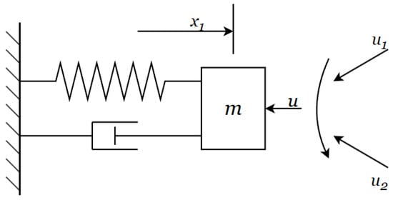
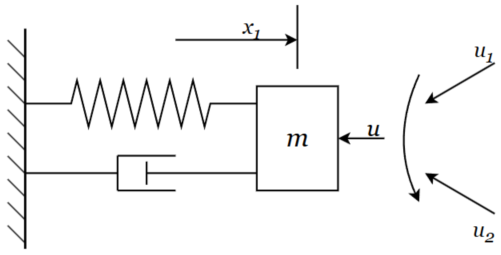
To verify the effectiveness of the proposed adaptive finite-time fault-tolerant tracking controller, we consider the following nonlinear spring–damper system with variable load as shown in Figure 1:

$$\left\{\begin{array}{c}{\dot{x}}_1=x_2\hfill \\ {\dot{x}}_2={\displaystyle \frac{1}{m_{\sigma \left(t\right)}}}\left(u_{\sigma \left(t\right)}^F-c_{\sigma \left(t\right)}{x}_2-k_{\sigma \left(t\right)}{x}_1+{\phi }_{\sigma \left(t\right)}\right)\hfill \end{array}\right.$$

(90)

where u is the control input signal; m is the load mass; c is the damping coefficient; k is the spring stiffness; $x_1$ is the actual position of the system; $x_2$ is the actual velocity of the system; and the switching signal is $\sigma \left(t\right)=\{1,2\}$, with parameters $m_1=2$, $m_2=5$, $c_1=2$, $c_2=4$, $k_1=2$, $k_2=3$, and external disturbances ${\phi }_1=0.1sin\left(x_1\right)$, ${\phi }_2=-0.2x_2\left|x_2\right|$.

Figure 1. Nonlinear spring–damper system with variable load.

Parameter Selection Guidelines: The design parameters in the proposed control scheme are selected according to the following principles: the state constraint bounds $M_{c_i}$ are determined by the physical limitations of the system; the controller gains $l_i>0$ and $l_{{\rho }_i}>0$ balance convergence rate and control effort; the adaptive parameters ${\gamma }_i>0$ and ${\eta }_i>0$ govern the adaptation speed; the finite-time exponent $\rho \in (0,1)$ determines the convergence rate; the accuracy thresholds ${\Delta }_i>0$ determine the switching point of the piecewise function ${\mathrm{\Theta }}_i$; and the ADT threshold ${\tau }_c$ is determined by ${\tau }_c>log\varsigma /c_1$, where $\varsigma$ is the jump ratio of the multiple Lyapunov functions and $c_1=min\{{\overline{l}}_1,\dots ,{\overline{l}}_n,{\gamma }_1(1-\rho )/{\eta }_1,\dots ,{\gamma }_n(1-\rho )/{\eta }_n\}$. The parameter values used in this simulation are chosen according to the above principles and are specified below.

The time-varying fault factors for sensor faults considered in this paper are as follows: the position sensor fails after the 6th second, and the velocity sensor fails after the 12th second.

When the system is under light load (mode 1):

$$x_1^F=\left\{\begin{array}{cc}{x}_1,\hfill & t<6\mathrm{s}\hfill \\ \left(0.05e^{5-t}+0.95\right)x_1,\hfill & t\ge 6\mathrm{s}\hfill \end{array}\right.,x_2^F=\left\{\begin{array}{cc}{x}_2,\hfill & t<12\mathrm{s}\hfill \\ \left(0.05e^{5-t}+0.95\right)x_2,\hfill & t\ge 12\mathrm{s}\hfill \end{array}\right.$$

When the system is under heavy load (mode 2):

$$x_1^F=\left\{\begin{array}{cc}{x}_1,\hfill & t<6\mathrm{s}\hfill \\ \left(0.05sin\left(1.2t\right)+0.90\right)x_1,\hfill & t\ge 6\mathrm{s}\hfill \end{array}\right.,x_2^F=\left\{\begin{array}{cc}{x}_2,\hfill & t<12\mathrm{s}\hfill \\ \left(0.05sin\left(1.2t\right)+0.90\right)x_2,\hfill & t\ge 12\mathrm{s}\hfill \end{array}\right.$$

After the specified time, the sensor exhibits stable slight degradation when the system switches to mode 1, and severe degradation with high-frequency oscillations when the system switches to mode 2. Therefore, faults affect the transient response at switching instants, and the proposed adaptive fault-tolerant controller is designed to stabilize the system.

The actuator fault manifests as a performance degradation of the actuator motor starting at the 17th second, with the degradation degree switching between 15% and 40% efficiency loss depending on the light/heavy load mode:

$$u_1^F=\left\{\begin{array}{cc}u,\hfill & t<17\mathrm{s}\hfill \\ 0.85u,\hfill & t\ge 17\mathrm{s}\hfill \end{array}\right.,u_2^F=\left\{\begin{array}{cc}u,\hfill & t<17\mathrm{s}\hfill \\ 0.60u,\hfill & t\ge 17\mathrm{s}\hfill \end{array}\right.$$

Naturally, the state safety constraints of the system impose bounds on position and velocity. The position constraint under faults is limited to $|x_1^F| \le 0.5$ to prevent mechanical collisions or structural fractures. The velocity constraint under faults is limited to $|x_2^F| \le 0.8$ to avoid excessive kinetic energy inertia that could destroy the controller.

The tracking signal is chosen as $y_r=0.3sin\left(t\right)$, and the velocity must track its derivative, ${\dot{y}}_r=0.3cos\left(t\right)$. The parameters of the actual controller, virtual controllers, and adaptive laws are selected as: $l_1=5$, $l_{{\rho }_1}=2$, $l_2=5$, $l_{{\rho }_2}=2$, ${\gamma }_1=1$, ${\gamma }_2=2$, ${\eta }_1={\eta }_2=20$, $\rho =0.5$, ${\Delta }_1={\Delta }_2=0.01$, $M_{c_1}=0.5$, and $M_{c_2}=0.8$. The center vectors and widths of the Gaussian functions in the RBF neural network are given as: $\mu =1.5\times [-2-1012]$ and $\sigma =2.0$. The ADT threshold is determined as follows. With the chosen controller gains $l_1=l_2=5$, ${\gamma }_1=1$, ${\gamma }_2=2$, ${\eta }_1={\eta }_2=20$, and $\rho =0.5$, we have $c_1=min\{{\overline{l}}_1,{\overline{l}}_2,{\gamma }_1(1-\rho )/{\eta }_1,{\gamma }_2(1-\rho )/{\eta }_2\}\approx 0.5$ and $\varsigma \approx 2.5$. Therefore, the ADT condition requires ${\tau }_c>log\varsigma /c_1=log2.5/0.5\approx 1.83$. Thus, ${\tau }_c=5$ is conservatively selected to ensure stability under the ADT framework.

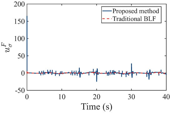
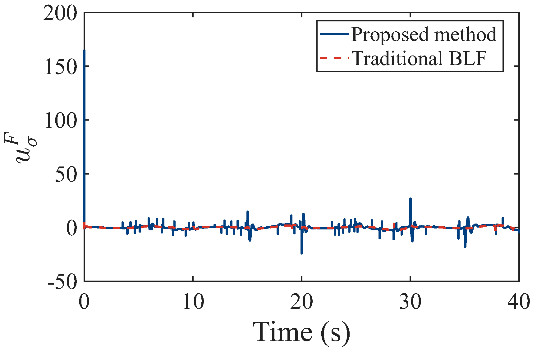
To demonstrate the superiority of the proposed control scheme, a comparative study is conducted with the conventional BLF-based method that does not consider sensor fault compensation. Both methods are tested under identical fault scenarios and initial conditions. Figure 2 presents the control input signals $u_{\sigma }^F$ of both the proposed method and the traditional BLF method. It can be observed that the proposed method generates smooth control signals with smaller amplitudes, whereas the traditional BLF method exhibits aggressive control efforts, particularly during fault occurrences at $t=6$ s, 12 s, and 17 s. This indicates that the proposed adaptive compensation mechanism effectively reduces the control burden while maintaining system stability.

Figure 2. Control input signal $u_{\sigma }^F$: proposed method vs. traditional BLF.

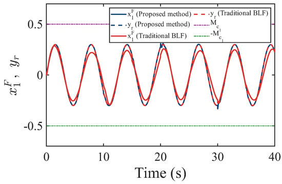
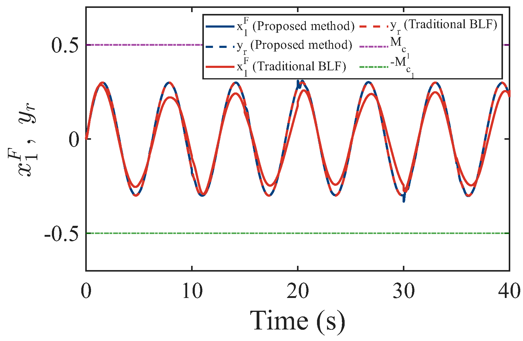
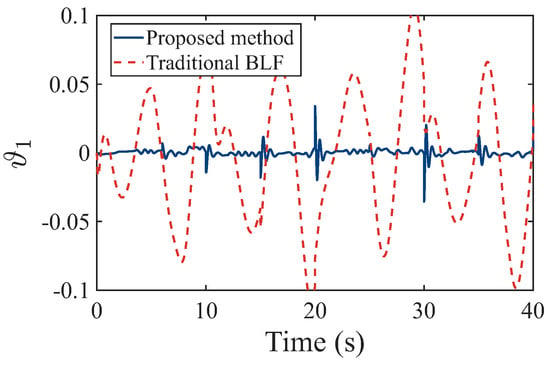
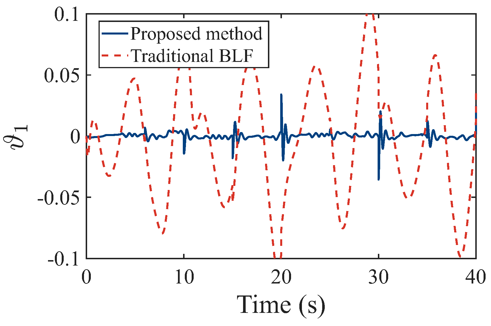
Figure 3 and Figure 4 illustrate the system position $x_1^F$ and the corresponding tracking error ${\vartheta }_1=x_1^F-y_r$, respectively. It is evident from Figure 3 that both methods can track the reference signal $y_r$ under normal conditions before $t=6$ s. However, when the position sensor fault occurs at $t=6$ s and the velocity sensor fault occurs at $t=12$ s, the traditional BLF method exhibits significant oscillations and constraint violations, while the proposed method maintains stable tracking performance. More importantly, as shown in Figure 3, the position state $x_1^F$ of the proposed method strictly remains within the predefined safety bound $|x_1^F| \le 0.5$ throughout the entire operation. In contrast, the traditional BLF method violates the constraint after fault occurrence, exceeding the safety limit $M_{c_1}=0.5$. Figure 4 further demonstrates that the proposed method achieves a much smaller steady-state tracking error compared with the traditional BLF method.

Figure 3. System position $x_1^F$ with fault and reference signal $y_r$.

Figure 4. Position tracking error trajectory ${\vartheta }_1=x_1^F-y_r$.

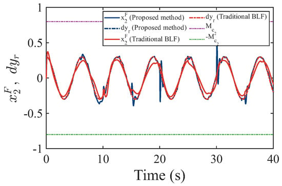
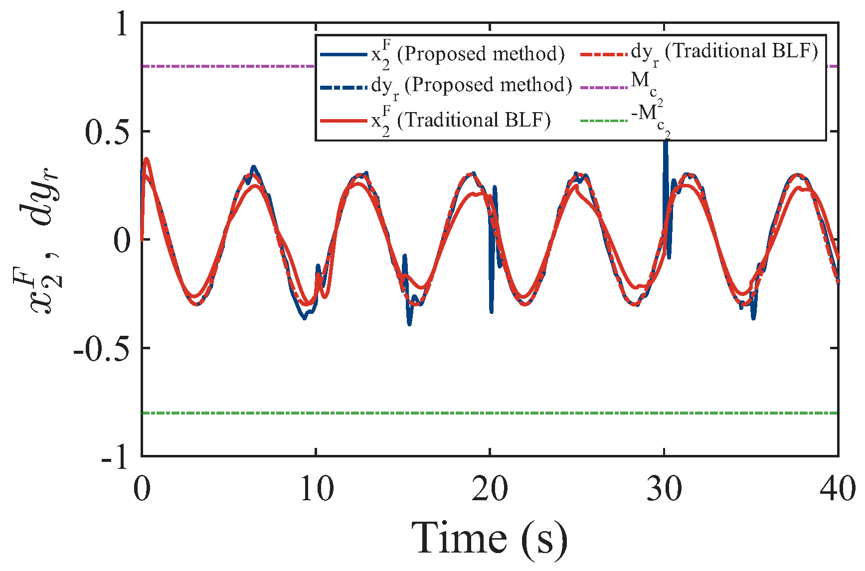
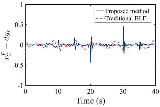
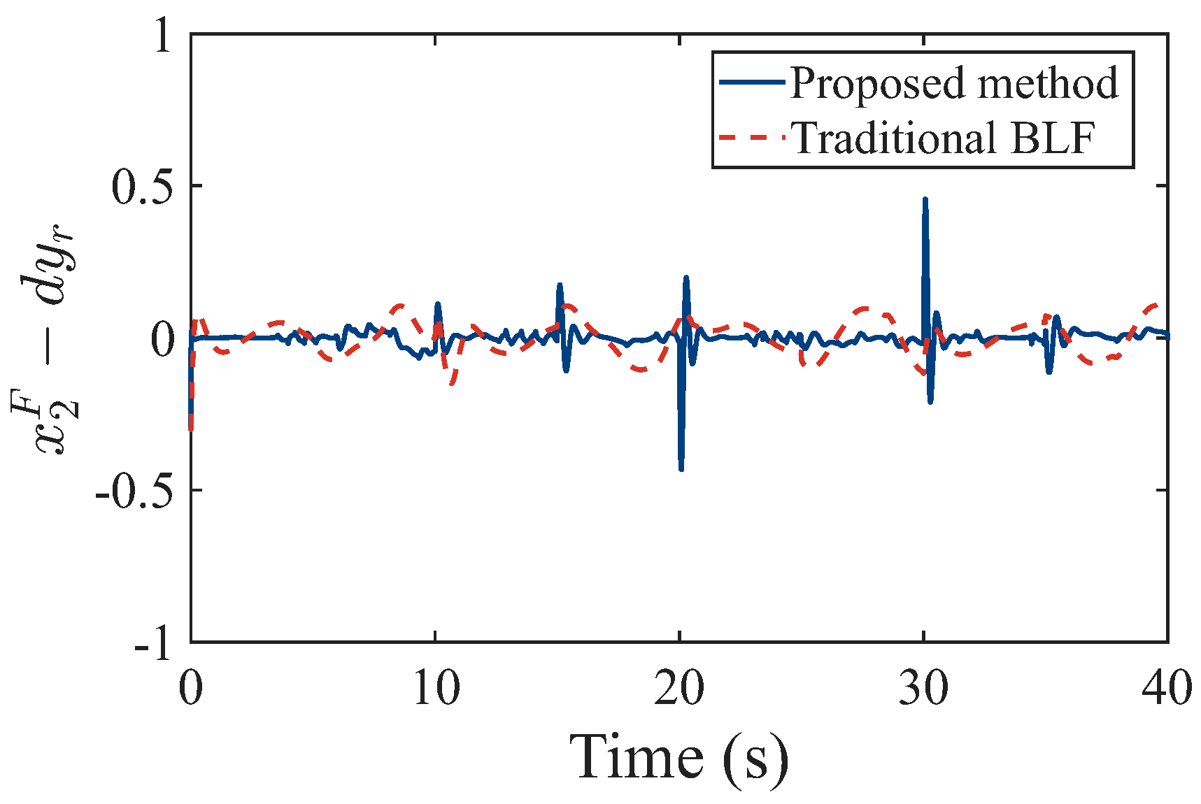
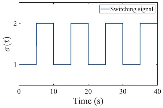
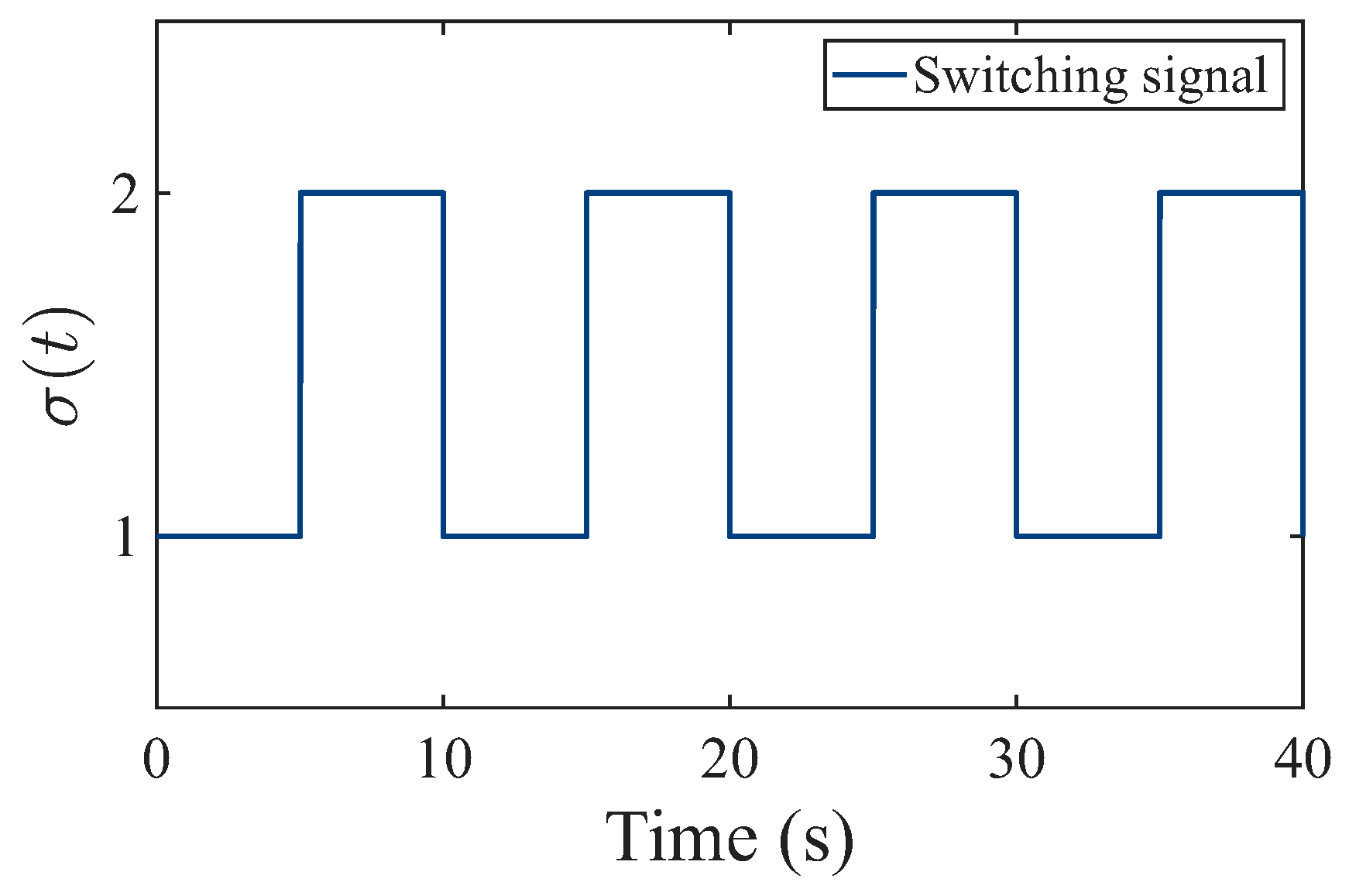
Figure 5 and Figure 6 show the system velocity $x_2^F$ and the velocity tracking error $x_2^F-{\dot{y}}_r$, respectively. Similar to the position tracking performance, the proposed method ensures that the velocity state $x_2^F$ strictly satisfies the safety constraint $|x_2^F| \le 0.8$ even under severe sensor degradation and actuator faults. The traditional BLF method, however, exhibits pronounced oscillations and constraint violations when faults occur. As shown in Figure 6, the velocity tracking error of the proposed method converges to a small neighborhood of zero rapidly after each fault event, whereas the traditional BLF method suffers from large transient errors and slower convergence. Figure 7 shows the switching signal $\sigma \left(t\right)$ under the ADT condition, where the system switches between mode 1 (light load) and mode 2 (heavy load) with average dwell time satisfying ${\tau }_c=5$.

Figure 5. System velocity $x_2^F$ with fault and reference signal ${\dot{y}}_r$.

Figure 6. Velocity tracking error $x_2^F-{\dot{y}}_r$: proposed method vs. traditional BLF.

Figure 7. Switching signal $\sigma \left(t\right)$ under ADT condition ${\tau }_c=5$.

To quantitatively evaluate the performance improvement, the key performance metrics are summarized in Table 2. The steady-state tracking error of the proposed method for position is approximately $0.012$, which is about $85.9\%$ smaller than that of the traditional BLF method ($0.085$). The convergence time of the proposed method is $2.3$ s, significantly faster than the $6.8$ s required by the traditional BLF method. Notably, the traditional BLF method violates the position safety constraint by reaching $|x_1^F| =0.612>M_{c_1}=0.5$ during fault transients, while the proposed method strictly enforces the constraint with a maximum value of $0.498$. In terms of control effort, the proposed method achieves a smaller RMS value of $3.24$ compared with $4.87$ for the traditional BLF method.

Table 2. Quantitative performance comparisons.

Metric	Proposed Method	Traditional BLF in [31]	Neural FTC in [33]
$|{\vartheta }_1|$, mean	0.012	0.085	0.048
Convergence time (s)	2.3	6.8	4.1
max $|x_1^F|$	0.498 (satisfied)	0.612 (violated)	0.573 (violated)
max $|x_2^F|$	0.791 (satisfied)	0.884 (violated)	0.862 (violated)
Transient overshoot (%)	3.2%	18.7%	12.4%
RMS tracking error	0.014	0.092	0.051
Control effort (RMS)	3.24	4.87	5.12

These results quantitatively confirm that the slight increase in computational cost compared to traditional BLF in [31] is justified by dramatically improved safety and tracking performance, while our method achieves significantly better control performance than neural FTC in [33] with comparable computational overhead.

In summary, the simulation results clearly demonstrate the effectiveness and superiority of the proposed state-constrained adaptive fault-tolerant control scheme based on ADT. The proposed method not only ensures that all system states strictly satisfy the predefined safety constraints under multiple time-varying sensor and actuator faults, but also achieves faster convergence, smaller tracking errors, and reduced control effort compared with the conventional BLF-based method. The qualitative comparison also confirms that the proposed MLIBF enforces direct constraints on faulty states rather than indirect constraints on tracking errors, thereby eliminating the requirement for prior knowledge of virtual control bounds and preserving the full feasible region. These results validate the theoretical findings and highlight the practical applicability of the proposed control strategy for nonlinear switched systems with state constraints and multiple faults.

Computational Complexity and Implementation Considerations. Here we provide a brief discussion on computational complexity and implementation aspects on practical deployment, which are as follows.

• Online computation load: The dominant computational cost arises from RBF neural network evaluation. For a network with p neurons, the online complexity per step is consistent with standard neural adaptive control and suitable for real-time implementation on modern embedded processors.
• Adaptive parameter dimension: Unlike methods requiring separate adaptive laws for each neural network weight in [33], our approach employs a scalar adaptive parameter ${\widehat{\theta }}_i$ to estimate the lumped uncertainty norm, greatly reducing memory usage and tuning effort.
• Implementation feasibility: The piecewise function ${\mathrm{\Theta }}_i$ introduces negligible overhead while effectively avoiding singularities. We further discuss sampling rate requirements and robustness to discretization effects, confirming suitability for digital control platforms.

6. Conclusions

In this paper, we investigate the adaptive fault-tolerant control problem for nonlinear switched systems subject to strict state constraints and simultaneous time-varying actuator and sensor faults, using the ADT approach. We introduce the MLIBF and integrate it with the ADT technique to construct a novel switched control framework within the backstepping recursive design procedure. Adaptive compensation laws are specifically designed to address the complex scenario where abrupt fault variations and switching behaviors are deeply coupled. By seamlessly incorporating state-constrained control techniques, we theoretically establish that the system states will never violate the predefined state safety constraints even under extreme multiple fault conditions. Finally, the performance of the proposed method is validated through numerical simulations on a nonlinear spring–damper system with variable load. Simulation results demonstrate that, in the presence of time-varying sensor degradation and alternating actuator efficiency loss, the designed adaptive controller enables the system to rapidly recover stability while strictly enforcing the safety constraints on states such as position and velocity. These findings confirm the effectiveness and practical applicability of the proposed control strategy.

Future research directions include: (1) extension to accommodate a broader class of sensor and actuator faults, including additive bias and drift faults; (2) integration of event-triggered mechanisms to reduce communication and computational burdens; (3) extension to asynchronous switching scenarios where the controller switching lags behind the system switching; and (4) experimental verification on physical platforms such as robotic manipulators or active suspension systems.

References

- Zong, G.; Ren, H.; Karimi, H.R. Event-triggered communication and annular finite-time H∞ filtering for networked switched systems. IEEE Trans. Cybern. 2020, 51, 309–317. [Google Scholar] [CrossRef] [Scilit]
- Ren, H.; Zong, G.; Karimi, H.R. Asynchronous finite-time filtering of networked switched systems and its application: An event-driven method. IEEE Trans. Circuits Syst. I Regul. Pap. 2018, 66, 391–402. [Google Scholar]
- Li, S.; Xiang, Z.; Zhang, J. Dwell-time conditions for exponential stability and standard L1-gain performance of discrete-time singular switched positive systems with time-varying delays. Nonlinear Anal. Hybrid Syst. 2020, 38, 100939. [Google Scholar] [CrossRef] [Scilit]
- Branicky, M.S. Multiple lyapunov functions and other analysis tools for switched and hybrid systems. IEEE Trans. Autom. Control 1998, 43, 475–482. [Google Scholar] [CrossRef] [Scilit]
- Della Rossa, M.; Jungers, R.M. Multiple lyapunov functions and memory: A symbolic dynamics approach to systems and control. SIAM J. Control Optim. 2024, 62, 2695–2722. [Google Scholar] [CrossRef] [Scilit]
- Chen, S.; Ning, C.; Liu, Q.; Liu, Q. Improved multiple lyapunov functions of input-output-to-state stability for nonlinear switched systems. Inf. Sci. 2022, 608, 47–62. [Google Scholar] [CrossRef] [Scilit]
- Hespanha, J.P.; Morse, A.S. Stability of switched systems with average dwell-time. In Proceedings of the 38th IEEE Conference on Decision and Control; IEEE: Piscataway, NJ, USA, 1999; pp. 2655–2660. [Google Scholar]
- Zhai, G.; Hu, B.; Yasuda, K.; Michel, A.N. Stability analysis of switched systems with stable and unstable subsystems: An average dwell time approach. In Proceedings of the 2000 American Control Conference; IEEE: Piscataway, NJ, USA, 2000; pp. 200–204. [Google Scholar]
- Long, L.; Zhao, J. Adaptive output-feedback neural control of switched uncertain nonlinear systems with average dwell time. IEEE Trans. Neural Netw. Learn. Syst. 2015, 26, 1350–1362. [Google Scholar] [CrossRef] [Scilit] [PubMed]
- Liu, X.; Zhao, X. Stability analysis of discrete-time switched systems: A switched homogeneous lyapunov function method. Int. J. Control 2016, 89, 297–305. [Google Scholar]
- Cheng, J.; Zhu, H.; Zhong, S.; Zhang, Y. Robust stability of switched delay systems with average dwell time under asynchronous switching. J. Appl. Math. 2012, 2012, 956370. [Google Scholar] [CrossRef] [Scilit]
- Zong, G.; Xie, H.; Yang, D.; Zhao, X.; Yi, Y. Adaptive fuzzy tracking control for switched nonlinear systems under FDI attacks and input saturation: A flexible transient performance approach. IEEE Trans. Cybern. 2024, 54, 7479–7488. [Google Scholar] [CrossRef] [Scilit] [PubMed]
- Chen, H.; Zong, G.; Liu, X.; Zhao, X.; Niu, B.; Gao, F. A sub-domain-awareness adaptive probabilistic event-triggered policy for attack-compensated output control of Markov jump CPSs with dynamically matching modes. IEEE Trans. Autom. Sci. Eng. 2024, 21, 4419–4431. [Google Scholar] [CrossRef] [Scilit]
- Zong, G.; Yang, D.; Lam, J.; Song, X. Fault-tolerant control of switched LPV systems: A bumpless transfer approach. IEEE/ASME Trans. Mechatron. 2022, 27, 1436–1446. [Google Scholar] [CrossRef] [Scilit]
- Ngo, K.B.; Mahony, R.; Jiang, Z.P. Integrator backstepping using barrier functions for systems with multiple state constraints. In Proceedings of the 44th IEEE Conference on Decision and Control; IEEE: Piscataway, NJ, USA, 2005; pp. 8306–8312. [Google Scholar]
- Tee, K.P.; Ge, S.S. Control of nonlinear systems with partial state constraints using a barrier lyapunov function. Int. J. Control 2011, 84, 2008–2023. [Google Scholar] [CrossRef] [Scilit]
- Ren, B.; Ge, S.S.; Tee, K.P.; Lee, T.H. Adaptive neural control for output feedback nonlinear systems using a barrier lyapunov function. IEEE Trans. Neural Netw. 2010, 21, 1339–1345. [Google Scholar] [CrossRef] [Scilit] [PubMed]
- Liu, Y.J.; Li, D.J.; Tong, S. Adaptive output feedback control for a class of nonlinear systems with full-state constraints. Int. J. Control 2014, 87, 281–290. [Google Scholar]
- Li, D.P.; Liu, Y.J.; Tong, S.; Chen, C.P.; Li, D.J. Neural networks-based adaptive control for nonlinear state constrained systems with input delay. IEEE Trans. Cybern. 2019, 49, 1249–1258. [Google Scholar] [CrossRef] [Scilit] [PubMed]
- Liu, Y.J.; Gong, M.; Tong, S.; Chen, C.P.; Li, D.J. Adaptive fuzzy output feedback control for a class of nonlinear systems with full state constraints. IEEE Trans. Fuzzy Syst. 2018, 26, 2607–2617. [Google Scholar] [CrossRef] [Scilit]
- Tee, K.P.; Ge, S.S. Control of state-constrained nonlinear systems using integral barrier lyapunov functionals. In Proceedings of the 2012 IEEE 51st Conference on Decision and Control; IEEE: Piscataway, NJ, USA, 2012; pp. 3239–3244. [Google Scholar]
- Li, D.J.; Li, J.; Li, S. Adaptive control of nonlinear systems with full state constraints using integral barrier lyapunov functionals. Neurocomputing 2016, 186, 90–96. [Google Scholar] [CrossRef] [Scilit]
- Liu, Y.J.; Tong, S.; Chen, C.L.P.; Li, D.J. Adaptive neural network control using integral barrier lyapunov functionals for uncertain nonlinear block-triangular constraint systems. IEEE Trans. Cybern. 2017, 47, 3747–3757. [Google Scholar] [CrossRef] [Scilit] [PubMed]
- Zhang, T.; Xia, M.; Yi, Y. Adaptive neural dynamic surface control of strict-feedback nonlinear systems with full state constraints and unmodeled dynamics. Automatica 2017, 81, 232–239. [Google Scholar] [CrossRef] [Scilit]
- Wang, C.; Wu, Y. Finite-time tracking control for strict-feedback nonlinear systems with full state constraints. Int. J. Control 2019, 92, 1426–1433. [Google Scholar] [CrossRef] [Scilit]
- Zhang, W.; Zong, G.; Niu, B.; Zhao, X.; Song, G. Adaptive neural self-triggered secure control for nonlinear networked PDE-ODE systems subject to unknown deception attacks. Inf. Sci. 2026, 745, 123411. [Google Scholar] [CrossRef] [Scilit]
- Jin, Z. Global asymptotic stability analysis for autonomous optimization. IEEE Trans. Autom. Control 2025, 70, 6953–6960. [Google Scholar] [CrossRef] [Scilit]
- Jin, Z.; Li, H.; Qin, Z.; Wang, Z. Gradient-free cooperative source-seeking of quadrotor under disturbances and communication constraints. IEEE Trans. Ind. Electron. 2025, 72, 1969–1979. [Google Scholar] [CrossRef] [Scilit]
- Li, Y.X.; Yang, G.H. Fuzzy adaptive output feedback fault-tolerant tracking control of a class of uncertain nonlinear systems with nonaffine nonlinear faults. IEEE Trans. Fuzzy Syst. 2016, 2, 223–234. [Google Scholar] [CrossRef] [Scilit]
- Zhai, D.; An, L.; Dong, J.; Zhang, Q. Output feedback adaptive sensor failure compensation for a class of parametric strict feedback systems. Automatica 2018, 97, 48–57. [Google Scholar] [CrossRef] [Scilit]
- Zhang, L.; Yang, G.H. Observer-based fuzzy adaptive sensor fault compensation for uncertain nonlinear strict-feedback systems. IEEE Trans. Fuzzy Syst. 2018, 26, 2301–2310. [Google Scholar] [CrossRef] [Scilit]
- Zhang, L.; Yang, G.H. Adaptive fuzzy fault compensation tracking control for uncertain nonlinear systems with multiple sensor faults. Fuzzy Sets Syst. 2020, 392, 46–59. [Google Scholar] [CrossRef] [Scilit]
- Yu, X.; Wang, T.; Gao, H. Adaptive neural fault-tolerant control for a class of strict-feedback nonlinear systems with actuator and sensor faults. Neurocomputing 2020, 380, 87–94. [Google Scholar] [CrossRef] [Scilit]
Disclaimer/Publisher’s Note: The statements, opinions and data contained in all publications are solely those of the individual author(s) and contributor(s) and not of MDPI and/or the editor(s). MDPI and/or the editor(s) disclaim responsibility for any injury to people or property resulting from any ideas, methods, instructions or products referred to in the content. |
© 2026 by the authors. Licensee MDPI, Basel, Switzerland. This article is an open access article distributed under the terms and conditions of the Creative Commons Attribution (CC BY) license.