A Hybrid PSO-GWO-BP Predictive Model for Demand-Driven Scheduling and Energy-Efficient Operation of Building Secondary Water Supply Systems

Abstract

Accurate forecasting of water demand enables optimized peak-load management, alleviating pressure during high-demand periods and improving the operational efficiency of urban secondary water supply systems—a critical component in the energy-efficient and sustainable operation of buildings. However, existing water demand prediction methods in some regions suffer from low accuracy and excessively long prediction cycles, posing challenges for real-time water scheduling in building-scale systems. To address these challenges, this study develops a hybrid predictive framework that integrates a BP neural network with the Gray Wolf Optimizer (GWO) and Particle Swarm Optimization (PSO) algorithms for enhanced parameter optimization. Using hourly water consumption data from a representative residential district, the proposed model is compared against standalone machine learning models—Extreme Learning Machines (ELM), Support Vector Machines (SVM), Long Short-Term Memory (LSTM), and Gated Recurrent Unit (GRU). Model performance is rigorously evaluated using the coefficient of determination, mean absolute error (MAE), mean squared error (MSE), mean absolute percentage error (MAPE), root mean square error (RMSE), and Nash–Sutcliffe efficiency coefficient (NSE). The PSO-GWO-BP hybrid model achieves a predictive accuracy of 97.06%, yielding the lowest MAE, MSE, RMSE, and MAPE, as well as the highest R among all models considered, thereby significantly outperforming the benchmark standalone models. Furthermore, the high-precision short-term prediction outputs enable dynamic regulation of secondary water tank refill thresholds, facilitating refined water allocation and enhanced operational management of building water supply systems. These findings demonstrate the considerable application potential of the proposed hybrid model in enhancing both water resource efficiency and energy utilization performance in the daily operation of green buildings, providing reliable technical support for intelligent and low-carbon building water supply management.

1. Introduction

Accurate prediction of urban residents’ water consumption is a pivotal prerequisite for efficient water resource allocation and intelligent operation of urban secondary water supply systems, which serve as core infrastructure for green residential buildings and building energy efficiency. In the context of sustainable urban development, the refined management of building-related water supply systems has become an important strategy for reducing operational energy consumption and improving resource utilization efficiency. However, current secondary water supply systems—particularly those serving residential buildings—face prominent challenges, including excessive pressure and volume surges during peak periods, as well as unstable water quality and low operational efficiency caused by delayed and unscientific scheduling [1]. These issues not only affect daily water use but also contribute to unnecessary energy losses, contradicting the low-carbon and sustainable operation goals of green buildings. Therefore, the development of efficient building water management strategies, high-precision short-term water demand prediction, and scientific real-time scheduling have become core priorities for optimizing secondary water supply systems, promoting building energy efficiency, and advancing green building operations [2].

Building on the need for high-precision prediction to optimize secondary water supply systems and support building energy efficiency, improving the accuracy of water consumption forecasts has become a key research focus. Statistical methods, known for their simplicity and ease of implementation, are widely employed to understand residents’ water consumption patterns [3]. For instance, Fullerton et al. [4] developed a linear transfer function (LTF) model to study water demand dynamics in El Paso. Yasar et al. [5] used stepwise multiple regression to identify key variables for a nonlinear water consumption model in Yadana City, Turkey. Gagliardi et al. [6] applied Markov chain-based methods to predict water demand within a 1–24 h horizon across three metered areas in the UK. Gharabaghi et al. [7] incorporated a data grouping technique into a nonlinear model, achieving a determination coefficient of 71.03 and a mean absolute percentage error of 2.93. However, statistical methods rely on large historical datasets and assume linearity and stability, making prediction accuracy highly dependent on data quality.

For non-stationary datasets or cases with multi-factor influences, machine learning methods can handle these challenges effectively due to their strong adaptability and nonlinear processing capabilities. Shan et al. [8] proposed a machine learning framework with dual feature filtering and the Maximum Information Coefficient (MIC) to enhance the accuracy and stability of short-term water demand forecasts. Bárdossy et al. [9] developed a hybrid fuzzy algorithm for multi-day water usage forecasting, achieving stable deviations of 5–6%, outperforming traditional statistical methods (5.5–10%). Smolak et al. [10] integrated human mobility data into a machine learning framework and achieved a best-model accuracy of 90.4%. Yu et al. [11] improved the Slime Mold Algorithm (SMA) with opposition-based learning and elite chaotic search, developing an enhanced ESMA algorithm that demonstrated fast, accurate, and robust convergence across linear, exponential, logarithmic, and hybrid forecasting models. Herrera et al. [12] compared various time-series forecasting models for urban water demand in southeastern Spain and found that Support Vector Regression (SVR) performed best, achieving a mean absolute error (MAE) of 4.33. Ensemble prediction models integrate the strengths of multiple algorithms, significantly improving training speed and prediction accuracy over single models. For instance, Asgarkhani et al. [13] developed a dynamic ensemble learning model using genetic algorithms and Particle Swarm Optimization to predict the nonlinear response and failure probability of steel frames under seismic loading, achieving a prediction accuracy of 99.3%. This highlights the strong potential of hybrid optimization and ensemble learning for complex engineering predictions.

Real-time scheduling of water volume is also a key issue that this research aims to address. To enhance the performance of real-time scheduling under uncertain perturbations, the current focus is on closed-loop control in the time domain [14]. Given the uncertainty associated with water volume scheduling over extended time periods, Xia et al. [15] proposed a multi-scale closed-loop framework that integrates real-time scheduling, achieving improved performance over longer time scales. Yuan et al. [16] developed a multi-timescale nested model to tackle the challenge of simultaneously optimizing long-term and short-term objectives, thereby improving the efficiency of water usage and resolving the trade-off between multiple objectives. Dini et al. [17] optimized pump operation scheduling to enhance the performance of water supply networks, introducing a novel method for optimizing the number of active pumps (NAPs) and their variable settings to achieve optimal scheduling. However, these studies and models are primarily designed for deterministic water use scenarios over extended time scales and lack real-time applicability.

A comparison of various machine learning algorithms for water quantity prediction modeling has been conducted to select an appropriate base model. Among these, BP neural networks offer strong parallel data processing and nonlinear mapping capabilities but suffer from slow training speeds, susceptibility to local optima, sensitivity to initial weights, and high data requirements [18]. In contrast, Extreme Learning Machines (ELMs) provide faster training and better generalization than Support Vector Machines (SVMs) in multi-classification tasks, yet their effectiveness is sensitive to manual parameter selection [19]. SVMs exhibit strong generalization, high-dimensional capability, and robustness to outliers, but face high computational complexity with large-scale datasets and require careful parameter tuning [20]. The Particle Swarm Optimization (PSO) algorithm is well-suited for multi-objective optimization problems due to its fast convergence rate and ability to avoid local optima, making it suitable for water consumption prediction in water supply systems. However, the performance of PSO is heavily dependent on the definition of the fitness function and parameter settings, which may require several adjustments to achieve optimal results [21]. The Gray Wolf Optimizer (GWO) features strong global search and fast convergence but is prone to local optima and high computational complexity in high-dimensional problems, with sensitivity to parameter settings [22].

Given the limitations of individual algorithms, this study aims to improve prediction accuracy by combining the strengths of multiple machine learning techniques to develop a hybrid prediction model. The key innovation of the proposed PSO-GWO-BP model lies in a tight coupling mechanism between PSO and GWO, rather than a simple sequential or parallel combination. This allows each wolf to retain its own best historical information while also learning from the three leader wolves, thereby avoiding the premature convergence of GWO and the local optima trap of PSO. The proposed model leverages the parallel data processing and nonlinear simulation capabilities of BP neural networks, incorporating both the PSO and GWO algorithms to optimize the model’s parameters. Accurate prediction of residential water demand is achieved by adjusting the weights and thresholds of the neural network, minimizing output errors. To validate the superiority of the hybrid model, its prediction accuracy is compared against ELM, SVM, a standalone BP neural network, and the hybrid GWO-BP algorithm, as well as state-of-the-art deep learning models, LSTM and GRU. In terms of application, water scheduling in the secondary supply system can be achieved by adjusting the replenishment threshold level of the tank based on model predictions, enabling flexible regulation of water volume. By enabling high-precision hourly forecasts and dynamic tank level control, the proposed hybrid model helps reduce unnecessary pump starts and stops, thereby lowering the operational energy consumption of building water supply systems. This approach aligns with the objectives of green building operation and building energy efficiency, contributing to the intelligent and low-carbon management of building-scale water infrastructure.

2. Methods

Considering that the BP neural network possesses excellent nonlinear mapping capabilities, a flexible network structure, and has a solid theoretical foundation as well as robust performance, it is selected as the base model for developing the hybrid prediction model in this study. However, traditional parametric optimization methods, such as experimental, grid, and gradient descent methods, primarily reflect the local nature of the BP neural network and require the objective function to be continuously differentiable. This requirement limits their applicability to optimization problems [23]. To enhance the convergence speed and generalization ability of the neural network, intelligent algorithms with global search capabilities are often preferred over traditional optimization methods. One notable advantage of the Gray Wolf Optimizer (GWO) algorithm is its strong global search capability and fast convergence, making it well-suited for solving complex optimization problems. Therefore, GWO is chosen as the optimization method for the BP neural network in this study. Since GWO mainly focuses on enhancing global search capabilities, it is prone to getting trapped in local optima [24]. To address this issue, the PSO algorithm, which excels in local search, is introduced as a supplement to GWO. This hybrid approach balances both local and global search capabilities, thus improving the overall performance of the hybrid prediction model [25]. The Extreme Learning Machines (ELMs) offer fast learning speed and high generalization ability, while Support Vector Machines (SVMs) demonstrate significant advantages in handling high-dimensional data and nonlinear problems. To evaluate the performance of the hybrid prediction model in these aspects, a comparative analysis is conducted using ELM, SVM, and the hybrid model. The optimization effects are validated using empirical data.

2.1. Data Preprocessing

The water consumption data used for model training were obtained from flow monitoring systems at secondary water supply pumping stations in selected neighborhoods, while meteorological data were acquired from publicly available sources, such as the National Centers for Environmental Information (NCEI) website (https://www.ncei.noaa.gov/maps/hourly/, acccessed on 18 March 2024).

Outliers were detected using the Z-score method (threshold = 3), and values exceeding the threshold were capped at the 99th percentile to avoid interference from extreme values. Data normalization was performed using the mapminmax function in MATLAB (R2023b) to scale all features into the interval [y_min, y_max], ensuring that no single feature dominates the learning process due to differences in magnitude.

The water consumption dataset was divided into two subsets, the training set and the test set. The hourly water demand data for residential communities from 07:00 to 08:00 on 1 January 2023 to 23:00 to 24:00 on 29 June 2023 was used as the training set to fit the parameters of the model. The hourly water demand data for residential communities from 00:00 to 01:00 on 30 June 2023 to 23:00 to 24:00 on 30 June 2023 was used as the test set to evaluate the network’s performance.

The Pearson correlation coefficient (PCC) was selected as a statistical measure to quantify the correlation between variables. The absolute value of the PCC is in the range of [−1, 1], with higher values indicating stronger correlations [26].

2.2. Traditional Machine Learning Algorithms

• BP neural network (BPNN)

The BP neural network (BPNN) is a model that calculates the output error of neurons layer by layer, starting from the output layer, using error backpropagation [27]. It then fine-tunes the connection weights and thresholds of each layer through the gradient descent method to minimize the output error [28].

2.

Extreme Learning Machines (ELMs)

Extreme Learning Machines (ELMs) are a fast training algorithm for single hidden-layer feedforward neural networks (SLFNs). They optimize the iterative process by randomly initializing input weights and bias, and using Moore–Penrose generalized inverse matrix theory to analytically calculate output layer weights [29].

3.

Support Vector Machines (SVMs)

Support Vector Machines (SVMs) are binary classification models. The core concept of SVM is to find a linear hyperplane in the feature space that maximizes the margin, which is defined as the distance between the hyperplane and the nearest data points from either class. This hyperplane effectively separates the two classes by maximizing the margin, thereby improving classification performance.

4.

LSTM (Long Short-Term Memory)

Long Short-Term Memory (LSTM) is a specialized recurrent neural network (RNN) architecture designed to overcome the vanishing gradient problem that standard RNNs encounter when processing long sequences. Introduced by Hochreiter and Schmidhuber in 1997, LSTM incorporates a gated structure consisting of a cell state, an input gate, a forget gate, and an output gate, which allows the network to selectively retain or discard information over extended time intervals, thereby effectively learning long-term dependencies in sequential data [30].

5.

GRU (Gated Recurrent Unit)

Gated Recurrent Unit (GRU) is a simplified variant of recurrent neural networks. Compared to LSTM, it contains only two gates (a reset gate and an update gate), which reduces the number of parameters while retaining the ability to capture long-term dependencies in time series data [31]. Consequently, GRU offers faster training and higher computational efficiency, making it particularly attractive in resource-constrained scenarios.

6.

Particle Swarm Optimization (PSO)

The Particle Swarm Optimization (PSO) algorithm initializes a population of particles, each of which is characterized by two attributes: velocity and position, without mass or volume. Each particle updates its velocity and position based on its own best solution and the best solution found by the population through information sharing with the goal of finding the global optimum via continuous iterations [32].

7.

Gray Wolf Optimizer (GWO)

Within the Gray Wolf Optimizer (GWO) algorithm, wolves are categorized into four distinct ranks based on their relative positional advantages and disadvantages. The α wolves act as the leaders, issuing directives related to hunting, resting, and other critical decisions regarding the pack’s activities. The β wolves serve as subordinates to the α wolves, coordinating the actions of lower-ranking wolves and assisting in decision-making. The σ wolves play a key role in ensuring the pack’s safety, while the ω wolves are responsible for executing the decisions made by the α wolves. The position of the prey represents the global optimum solution [22]. The implementation steps for GWO are as follows:

Phase 1, Encircling Prey: When wolves find their prey, they gradually approach and encircle it. The mathematical model of this behavior is as follows:

$$\stackrel{\mathrm{⃑}}{\mathrm{D}} = \left|\stackrel{\mathrm{⃑}}{\mathrm{C}}·{\stackrel{\mathrm{⃑}}{\mathrm{X}}}_{\mathrm{p}}\left(\mathrm{t}\right)-\stackrel{\mathrm{⃑}}{\mathrm{X}}\left(\mathrm{t}\right)\right|$$

(1)

$$\stackrel{\mathrm{⃑}}{\mathrm{X}}\left(\mathrm{t}+1\right)={\stackrel{\mathrm{⃑}}{\mathrm{X}}}_{\mathrm{p}}\left(\mathrm{t}\right)-\stackrel{\mathrm{⃑}}{\mathrm{A}}·\stackrel{\mathrm{⃑}}{\mathrm{D}}$$

(2)

where $\stackrel{\mathrm{⃑}}{\mathrm{D}}$ denotes the distance between the prey and the gray wolf; t is the number of iterations; $\stackrel{\mathrm{⃑}}{\mathrm{C}}$ and $\stackrel{\mathrm{⃑}}{\mathrm{A}}$ are the coefficients; $\stackrel{\mathrm{⃑}}{\mathrm{X}}\left(\mathrm{t}\right)$ is the position vector of the gray wolf at generation t, and ${\stackrel{\mathrm{⃑}}{\mathrm{X}}}_{\mathrm{p}}\left(\mathrm{t}\right)$ is the position vector of the prey at generation t. The formulas for the vectors $\stackrel{\mathrm{⃑}}{\mathrm{A}}$ and $\stackrel{\mathrm{⃑}}{\mathrm{C}}$ are as follows:

$$\stackrel{\mathrm{⃑}}{\mathrm{A}} = 2·\stackrel{\mathrm{⃑}}{\mathsf{\alpha }}·{\stackrel{\mathrm{⃑}}{\mathrm{r}}}_1-\stackrel{\mathrm{⃑}}{\mathsf{\alpha }}$$

(3)

$$\stackrel{\mathrm{⃑}}{\mathrm{C}}=2·{\stackrel{\mathrm{⃑}}{\mathrm{r}}}_2$$

(4)

where ${\stackrel{\mathrm{⃑}}{\mathrm{r}}}_1$ and ${\stackrel{\mathrm{⃑}}{\mathrm{r}}}_2$ are random numbers in the interval [0, 1]. $\stackrel{\mathrm{⃑}}{\mathsf{\alpha }}$ serves as the control coefficient, which generally takes the value in the range [0, 2] and decreases linearly with the number of iterations.

Phase 2, Hunting: α wolves, who know the location of their prey best, lead β wolves and σ wolves on the hunt, and the other gray wolves update the position of α, β, and σ wolves in turn, as shown in this formula:

$${\stackrel{\mathrm{⃑}}{\mathrm{D}}}_{\mathsf{\alpha }} = \left|{\stackrel{\mathrm{⃑}}{\mathrm{C}}}_1·{\stackrel{\mathrm{⃑}}{\mathrm{X}}}_{\mathsf{\alpha }}-\stackrel{\mathrm{⃑}}{\mathrm{X}}\left(\mathrm{t}\right)\right|$$

(5)

$${\stackrel{\mathrm{⃑}}{\mathrm{D}}}_{\mathsf{\beta }}=\left|{\stackrel{\mathrm{⃑}}{\mathrm{C}}}_2·{\stackrel{\mathrm{⃑}}{\mathrm{X}}}_{\mathsf{\beta }}-\stackrel{\mathrm{⃑}}{\mathrm{X}}\left(\mathrm{t}\right)\right|$$

(6)

$${\stackrel{\mathrm{⃑}}{\mathrm{D}}}_{\mathsf{\sigma }}=\left|{\stackrel{\mathrm{⃑}}{\mathrm{C}}}_3·{\stackrel{\mathrm{⃑}}{\mathrm{X}}}_{\mathsf{\sigma }}-\stackrel{\mathrm{⃑}}{\mathrm{X}}\left(\mathrm{t}\right)\right|$$

(7)

$${\stackrel{\mathrm{⃑}}{\mathrm{X}}}_{\mathsf{\alpha }}\left(\mathrm{t}+1\right)={\stackrel{\mathrm{⃑}}{\mathrm{X}}}_{\mathsf{\alpha }}\left(\mathrm{t}\right)-{\stackrel{\mathrm{⃑}}{\mathrm{A}}}_1·{\stackrel{\mathrm{⃑}}{\mathrm{D}}}_{\mathsf{\alpha }}$$

(8)

$${\stackrel{\mathrm{⃑}}{\mathrm{X}}}_{\mathsf{\beta }}\left(\mathrm{t}+1\right)={\stackrel{\mathrm{⃑}}{\mathrm{X}}}_{\mathsf{\beta }}\left(\mathrm{t}\right)-{\stackrel{\mathrm{⃑}}{\mathrm{A}}}_2·{\stackrel{\mathrm{⃑}}{\mathrm{D}}}_{\mathsf{\beta }}$$

(9)

$${\stackrel{\mathrm{⃑}}{\mathrm{X}}}_{\mathsf{\sigma }}\left(\mathrm{t}+1\right)={\stackrel{\mathrm{⃑}}{\mathrm{X}}}_{\mathsf{\sigma }}\left(\mathrm{t}\right)-{\stackrel{\mathrm{⃑}}{\mathrm{A}}}_3·{\stackrel{\mathrm{⃑}}{\mathrm{D}}}_{\mathsf{\sigma }}$$

(10)

$$\stackrel{\mathrm{⃑}}{\mathrm{X}}\left(\mathrm{t}+1\right)={\displaystyle \frac{{\stackrel{\mathrm{⃑}}{\mathrm{X}}}_{\mathsf{\alpha }}\left(\mathrm{t}+1\right)+{\stackrel{\mathrm{⃑}}{\mathrm{X}}}_{\mathsf{\beta }}\left(\mathrm{t}+1\right)+{\stackrel{\mathrm{⃑}}{ \mathrm{X}}}_{\mathsf{\sigma }}\left(\mathrm{t}+1\right)}{3}}$$

(11)

where ${\stackrel{⃑}{X}}_{\alpha }\left(t\right)$, ${\stackrel{⃑}{X}}_{\beta }\left(t\right)$, ${\stackrel{⃑}{X}}_{\sigma }\left(t\right)$ and $\stackrel{⃑}{X}\left(t\right)$ denote the position vectors of $\alpha$, $\beta$, $\sigma$ and current wolves in the population.

Phase 3, Attack phase: capture the target and obtain the optimal solution. When the convergence factor $\stackrel{\mathrm{⃑}}{\mathsf{\alpha }}$ decreases linearly from 2 to 0, the value of $\stackrel{\mathrm{⃑}}{\mathrm{A}}$ varies in the range [−2, 2]. When $\left|\stackrel{\mathrm{⃑}}{\mathrm{A}}\right|$ ≥ 1, it means that the gray wolves are still in the global search phase, and when $\left|\stackrel{\mathrm{⃑}}{\mathrm{A}}\right|$ < 1, the wolf pack will launch an attack to capture the target that has been targeted for local search.

2.3. Improvement of the Hybrid Algorithm

• PSO-GWO

Due to the linear decrease in the parameter $\stackrel{⃑}{a}$, the GWO algorithm lacks the ability to balance global search and local exploitation, ignoring the information sharing between individual gray wolves. To address this problem, inertia weights ω are introduced:

$$\stackrel{\mathrm{⃑}}{\mathrm{D} }= \left|\stackrel{\mathrm{⃑}}{\mathrm{C}}·{\stackrel{\mathrm{⃑}}{\mathrm{X}}}_{\mathrm{p}}\left(\mathrm{t}\right)-\mathsf{\omega }\stackrel{\mathrm{⃑}}{\mathrm{X}}\left(\mathrm{t}\right)\right|$$

(12)

The higher the inertia weight, the better the particle’s velocity is maintained over the search interval. The introduction of inertia weight enhances the global optimization capability of the GWO algorithm but weakens its local optimization performance. To address the issue of the GWO algorithm being prone to local optima, the concept of velocity from the PSO algorithm is introduced to update the velocity and position of the gray wolf:

$${\stackrel{⃑}{v}}_i\left(t+1\right)=\omega {\stackrel{⃑}{v}}_i+{\stackrel{⃑}{C}}_1·{\stackrel{⃑}{r}}_1·\left({\stackrel{⃑}{X}}_{\alpha }\left(t+1\right)-\stackrel{⃑}{X}\left(t\right)\right)+{\stackrel{⃑}{C}}_2·{\stackrel{⃑}{r}}_2·\left({\stackrel{⃑}{X}}_{\beta }\left(t+1\right)-\stackrel{⃑}{X}\left(t\right)\right)+{\stackrel{⃑}{C}}_3·{\stackrel{⃑}{r}}_3·\left({\stackrel{⃑}{X}}_{\sigma }\left(t+1\right)-\stackrel{⃑}{X}\left(t\right)\right)$$

(13)

$$\stackrel{\mathrm{⃑}}{\mathrm{X}}\left(\mathrm{t}+1\right)=\stackrel{\mathrm{⃑}}{\mathrm{X}}\left(\mathrm{t}\right)+{\stackrel{\mathrm{⃑}}{ \mathrm{v}}}_{\mathrm{i}}\left(\mathrm{t}+1\right)$$

(14)

where ${\stackrel{⃑}{C}}_1$, ${\stackrel{⃑}{C}}_2$, and ${\stackrel{⃑}{C}}_3$ are the optimization parameters.

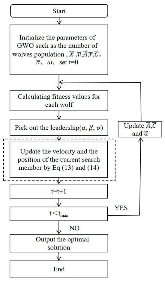
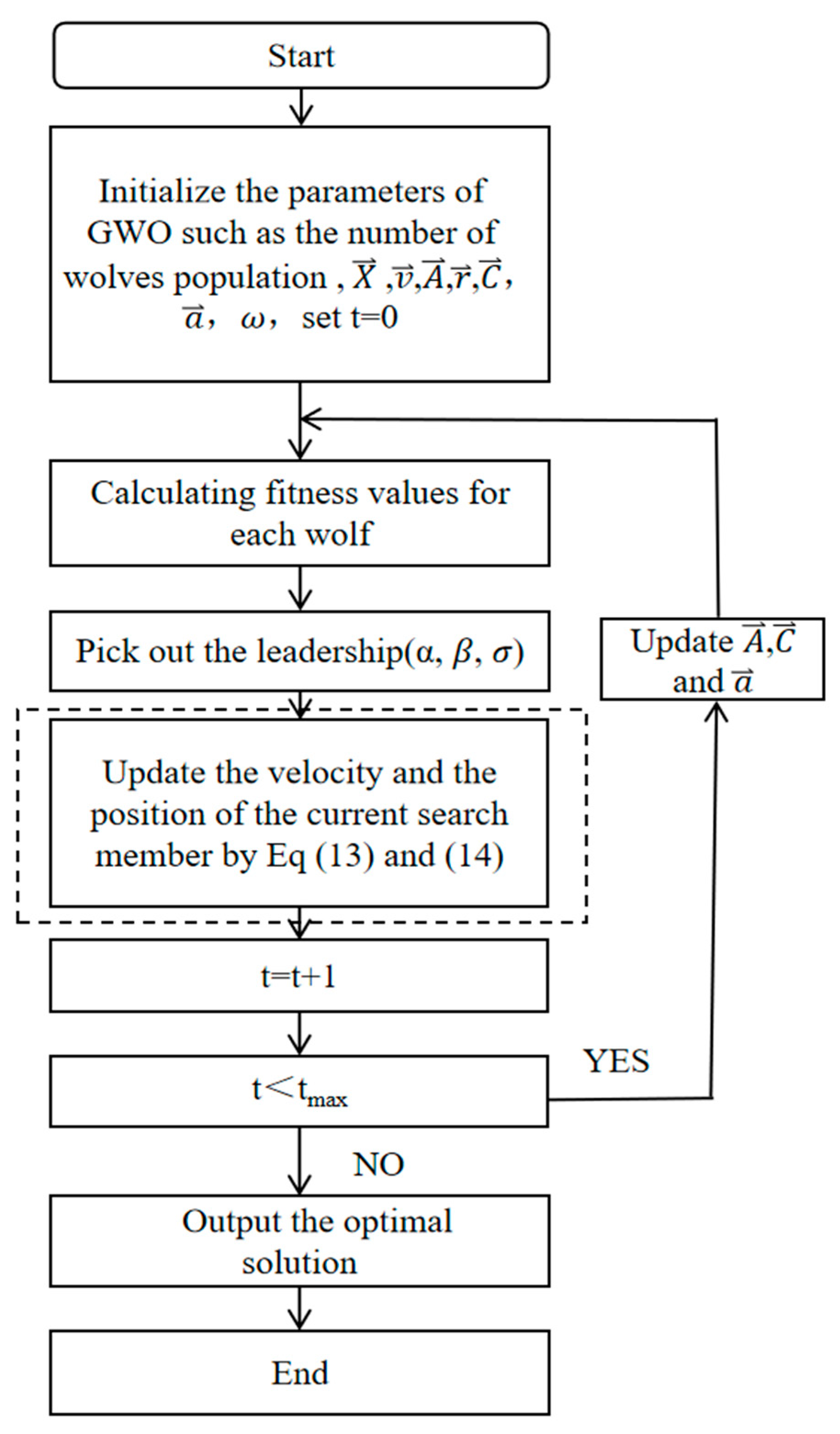
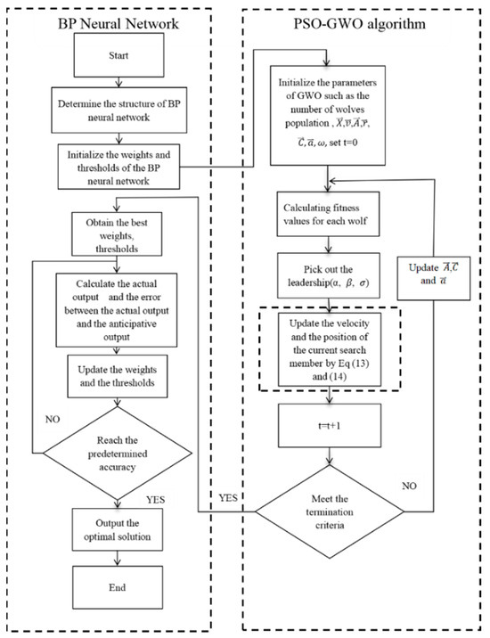
The specific processes of the PSO-GWO hybrid metaheuristic algorithm are shown in Figure 1.

Figure 1. Optimization process of the PSO-GWO algorithm.

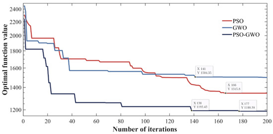
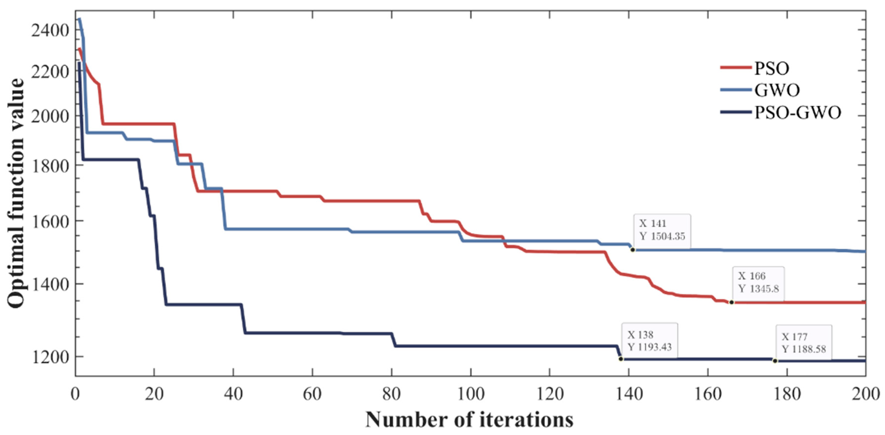
To evaluate the advantages of the improved GWO in parameter optimization, algorithm validation was performed using a standard PSO, a standard GWO, and a PSO-improved GWO on a test function. The number of iterations was used to assess the convergence speed of each predictive model.

As can be seen from Figure 2, during the 200 iterations of the experiment, PSO converges at iteration 166, reaching an optimal function value of 1345.8; GWO converges at iteration 141, with an optimal function value of 1504.35; and PSO-GWO stabilizes around iteration 138, and then fluctuates gradually, reaching an optimal function value of 1188.58 after 177 iterations. Throughout the test, PSO exhibited greater fluctuation compared to GWO and was less stable. While GWO achieved a higher optimal function value, its parameter optimization performance was suboptimal. In comparison, PSO-GWO required fewer iterations to stabilize, and its optimal function value was lower than that of both PSO and GWO, which indicates that the model is less likely to fall into local optima.

Figure 2. Iterative effect of test function of three intelligent algorithms.

The PSO-GWO algorithm exhibits rapid changes in the first 138 iterations, after which it stabilizes. This behavior can be attributed to the fact that PSO-GWO inherits the global search capability of the GWO, allowing the population to quickly converge to the global optimum. In the later stages, the integration of the PSO algorithm helps the population to concentrate rapidly around the optimal solution, reducing the probability of getting trapped in local optima, and thus balancing the exploration of global optima with the exploitation of local optima. Experimental results validate the superiority of the hybrid improved GWO in parameter optimization [33].

2.

PSO-GWO-BP

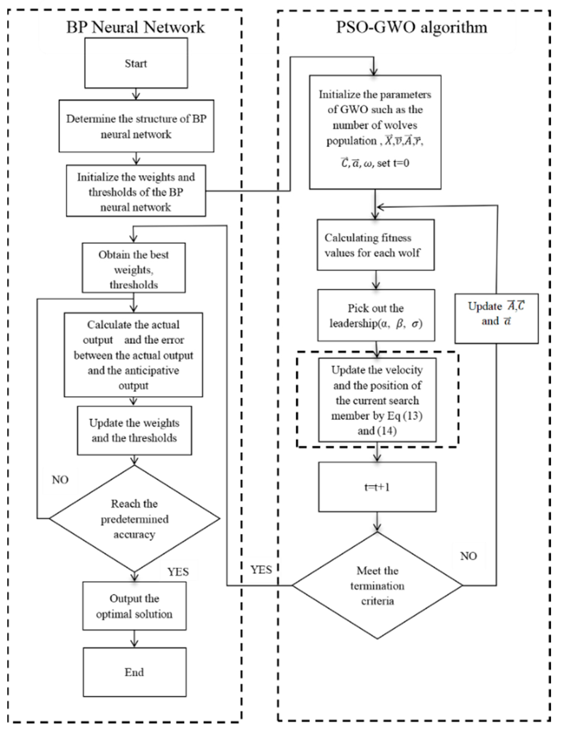
At each iteration of the PSO-GWO hybrid, each gray wolf’s position is updated using both the encircling mechanism from GWO (Equations (8)–(10)) and the velocity memory from PSO (Equations (13) and (14)). This tight coupling allows the wolf pack to benefit from GWO’s social hierarchy (α, β, and σ guiding the search) while simultaneously retaining individual historical best information via PSO’s velocity term. Consequently, the hybrid algorithm achieves faster convergence and a lower risk of falling into local optima compared to using either algorithm alone or in a simple sequential manner. The PSO-GWO-BP algorithm is then implemented to validate the improvement of the BP neural network using the hybrid optimization method. Firstly, the determination of the structure of the BP neural network is carried out, accompanied by the completion of the initialization of weights and thresholds. Subsequently, the hybrid PSO-GWO algorithm is invoked. The weights and thresholds of BP neural networks are regarded as optimization objectives. The algorithm was run to calculate the fitness of all gray wolf individuals, and the three gray wolves with the best fitness in the wolf pack were marked as α, β, and σ in turn, and the other wolf individuals were marked as ω. The wolves search for prey and perform encirclement operations, during which the positions and velocities of α, β, and σ wolves are updated according to Equations (5)–(10). The concept of particle velocity from the PSO algorithm is incorporated into the gray wolf position update, with each individual gray wolf treated as a particle in the swarm. The position and velocity updates for each gray wolf are shown in Equations (13) and (14). The termination condition is then evaluated, and if it is not met, the values of $\stackrel{⃑}{A}$, $\stackrel{⃑}{C}$, and $\stackrel{⃑}{a}$ are updated, and the process is repeated until the termination condition is satisfied. Once the termination condition is met, the optimal position within the gray wolf population is mapped to the initial weights and thresholds of the BP neural network. These optimal weights and thresholds are used to train the BP neural network. First, the output of the neural network is calculated. The error function is then used to calculate the error between the actual output and the expected output. Finally, the weights are adjusted to minimize the error until a satisfactory level of accuracy is achieved. The best value is then output.

The framework and execution process of PSO-GWO-BP are shown in Figure 3.

Figure 3. The flow chart of PSO-GWO-BP.

2.4. Model Performance Metrics

Assessment metrics are quantitative measures used to evaluate the accuracy of model predictions. Multiple metrics can be combined to assess the overall performance of a model after calibrating its structure [34]. To evaluate the prediction errors of different models, the mean absolute percentage error (MAPE), mean absolute error (MAE), mean squared error (MSE), root mean square error (RMSE), and Nash–Sutcliffe efficiency coefficient (NSE) are employed for comparison.

$$\mathrm{MAPE}={\displaystyle \frac{1}{\mathrm{n}}}\sum _{\mathrm{i}=1}^{\mathrm{n}}\left|{\displaystyle \frac{{\mathrm{y}}_{\mathrm{i}}-{\widehat{\mathrm{y}}}_{\mathrm{i}}}{{\widehat{\mathrm{y}}}_{\mathrm{i}}}}\right|\times 100\%$$

(15)

$$\mathrm{MAE}={\displaystyle \frac{1}{\mathrm{n}}}\sum _{\mathrm{i}=1}^{\mathrm{n}}\left|{\mathrm{y}}_{\mathrm{i}}-{\widehat{\mathrm{y}}}_{\mathrm{i}}\right|$$

(16)

$$\mathrm{MSE}={\displaystyle \frac{1}{\mathrm{n}}}\sum _{\mathrm{i}=1}^{\mathrm{n}}{\left({\mathrm{y}}_{\mathrm{i}}-{\widehat{\mathrm{y}}}_{\mathrm{i}}\right)}^2$$

(17)

$$\mathrm{R}\mathrm{M}\mathrm{S}\mathrm{E}=\sqrt{{\displaystyle \frac{1}{\mathrm{n}}}\sum _{\mathrm{i}=1}^{\mathrm{n}}{\left({\mathrm{y}}_{\mathrm{i}}-{\widehat{\mathrm{y}}}_{\mathrm{i}}\right)}^2}$$

(18)

$$\mathrm{N}\mathrm{S}\mathrm{E}=1-{\displaystyle \frac{\sum _{\mathrm{i}=1}^{\mathrm{n}}{\left({\mathrm{y}}_{\mathrm{i}}-{\widehat{\mathrm{y}}}_{\mathrm{i}}\right)}^2}{\sum _{\mathrm{i}=1}^{\mathrm{n}}{\left({\mathrm{y}}_{\mathrm{i}}-\stackrel{\mathrm{-}}{\mathrm{y}}\right)}^2}}$$

(19)

where $n$ is the number of data predicted; ${\widehat{y}}_i$ is the ith data actual value; $y_i$ is the ith data predicted value; and $\stackrel{\mathrm{-}}{\mathrm{y}}$ is the overall mean of the actual values.

2.5. Time-Series Cross-Validation Scheme

To rigorously evaluate the generalization ability of the proposed PSO-GWO-BP model and address the limitation of a single-day test set, we adopted an expanding window cross-validation strategy that respects the temporal order of water demand data. The entire dataset (1 January 2023 to 30 June 2023, 181 days, 4337 hourly records) was divided into five consecutive validation blocks, each containing 7 days (168 h). The splits are as follows:

• Fold 1: training on days 1–146, validation on days 147–153;
• Fold 2: training on days 1–153, validation on days 154–160;
• Fold 3: training on days 1–160, validation on days 161–167;
• Fold 4: training on days 1–167, validation on days 168–174;
• Fold 5: training on days 1–174, validation on days 175–181.

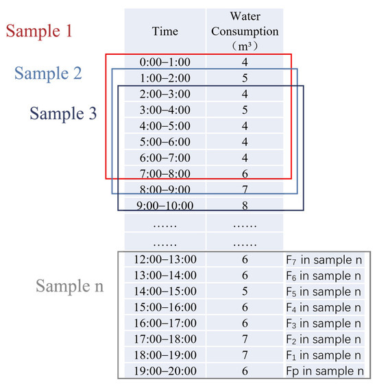
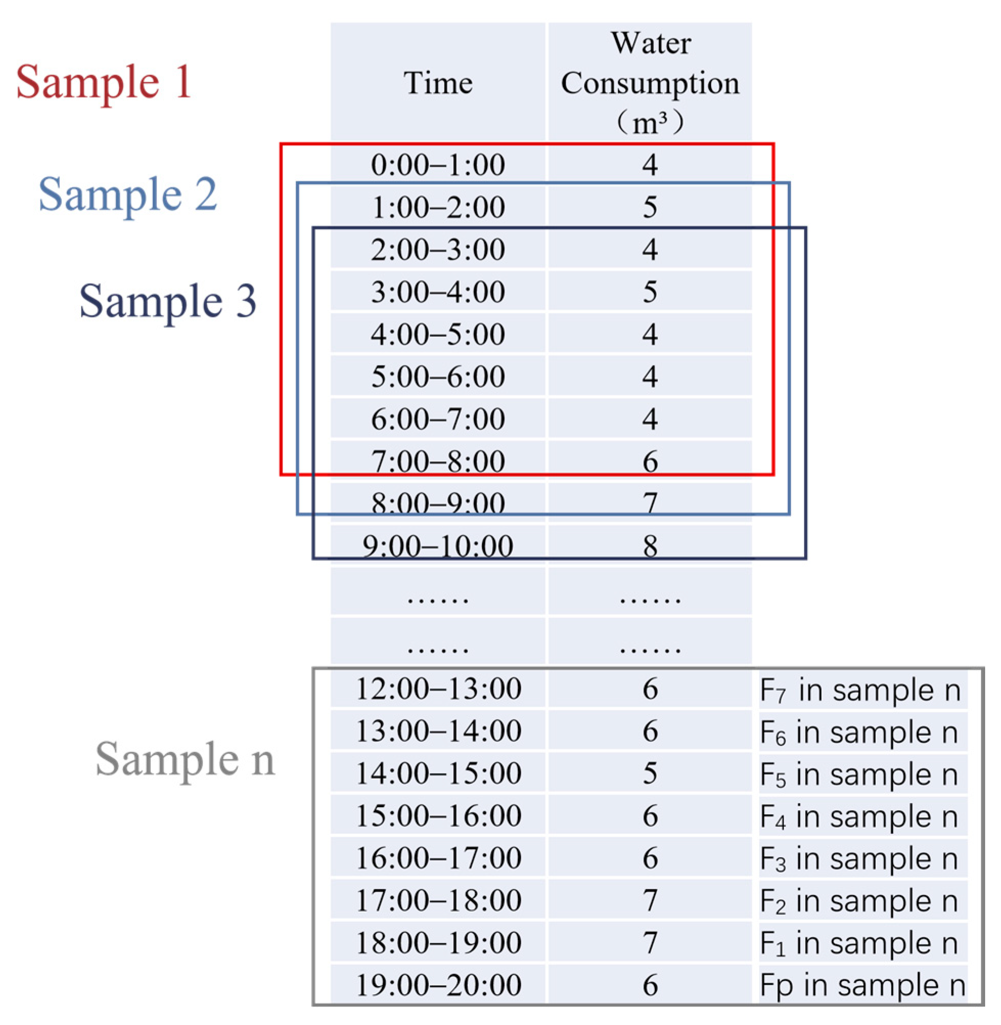
For each fold, the same 8 h sliding window (Figure 4) was applied to construct input–output samples from the training and validation periods. The PSO-GWO-BP model was retrained from scratch for each fold using identical hyperparameters (Table 1). The mean and standard deviation of the performance metrics (MAE, MSE, RMSE, MAPE, R, R², and NSE) across the five folds are reported to demonstrate model robustness.

Figure 4. Time series parameters schematic.

Table 1. The specific parameters of the models.

Model	Parameter	Type
PSO-GWO-BP	Number of neurons in hidden layer	10
	Activation function in input layer	Tansigmoidal activation function
	Activation function in hidden layer	Linear transfer function
	Learning algorithm	Levenberg–Marquardt
	Number of algorithm iterations	20
	Population size	3
	Number of model epochs	200
	Learning rate coefficient	0.01
GWO-BP	Number of neurons in hidden layer	10
	Activation function in input layer	Tansigmoidal activation function
	Activation function in hidden layer	Linear transfer function
	Learning algorithm	Levenberg–Marquardt
	Number of algorithm iterations	20
	Population size	3
	Number of model epochs	200
	Learning rate coefficient	0.01
BP	Number of neurons in hidden layer	5
	Activation function in input layer	Tansigmoidal activation function
	Activation function in hidden layer	Linear transfer function
	Learning algorithm	Levenberg–Marquardt
	Number of model epochs	200
	Learning rate coefficient	0.01
ELM	Number of neurons in hidden layer	20
	Transfer function	Sigmoidal function
	Number of model epochs	20
	Learning rate coefficient	0.01
SVM	Type of SVM	Epsilon-SVR
	Kernel function	Radial basis function
LSTM	Number of hidden units	64
	Optimizer	Adam
	Initial learning rate	0.01
	Max epochs	200
	Mini-batch size	32
GRU	Number of hidden units	64
	Optimizer	Adam
	Initial learning rate	0.01
	Max epochs	200
	Mini-batch size	32

The specific parameter settings for the models are presented in Table 1.

2.6. Water Scheduling Strategy

The water volume scheduling capability of the secondary water supply systems (SWSS) can be demonstrated by adjusting the proportion of recharge water volume from the tanks within the water supply system [35]. This study is grounded on the optimization model for predicting water consumption in the next period. Through pre-adjusting the refill level of the tank, the proportion of water replenishment is regulated. Specifically, prior to the arrival of the peak water consumption period, the inflow into the water tank is increased, while during the peak period, the inflow is reduced, thereby creating peaks and valleys in the tank inflow amount and realizing the real-time scheduling of the water supply volume of the tank.

3. Case Study

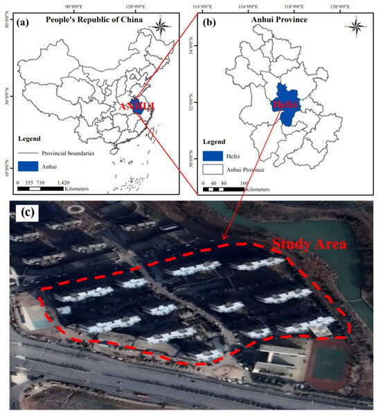
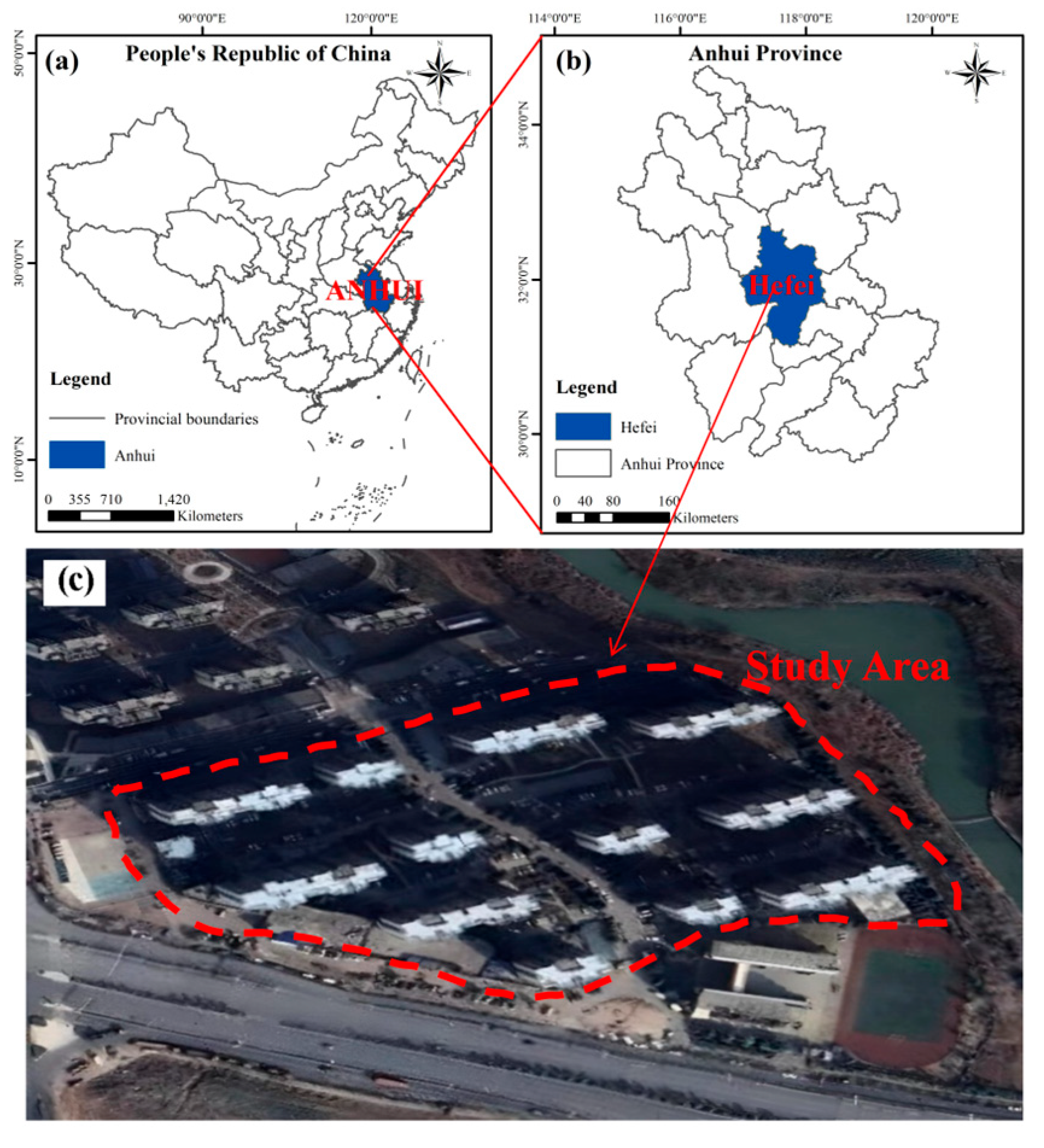
The living area selected for this study is shown in Figure 5 and is also surrounded by markets and schools. There are 12 residential buildings in the district, of which 1, 2, and 4 are 22 stories high, and the other buildings are 26 stories high. The number of housing households is 1844, and the scale is moderate. Most of the residents are office workers, leaving early and returning late. The household structure is mostly nuclear with regularity in water use activities. The original dataset is derived from the secondary water supply pump house of the neighborhood. This pump house is equipped with a flow monitoring platform that enables real-time data collection and transmission.

Figure 5. (a) Map showing the province where the research area is located; (b) Map showing the city where the research area is located; (c) Map showing the situation of the research area and its surrounding areas.

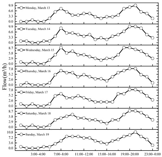
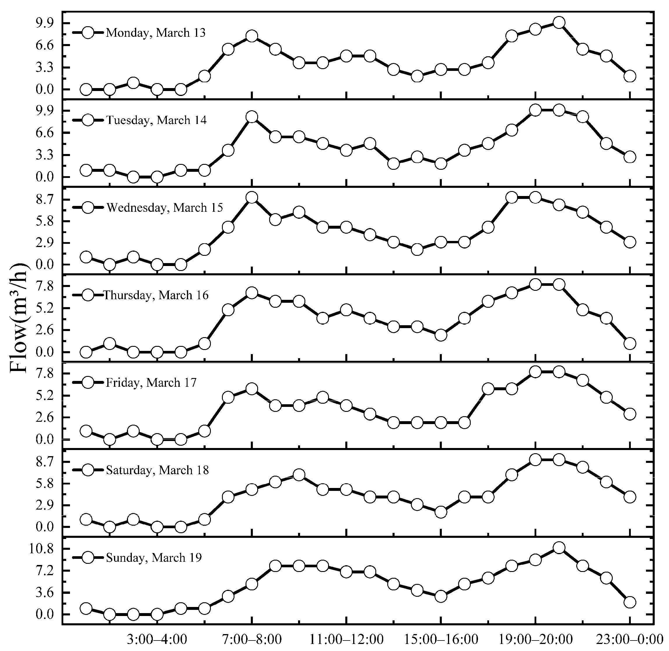
In order to study the effect of the time factor on water use in settlements, fluctuations in water use over a week were plotted based on the dataset.

As shown in Figure 6, the water usage patterns in this residential community are distinct. The variation in daily water consumption generally follows an M-shaped pattern. The morning peak on weekdays typically occurs between 07:00 and 08:00, while the evening peak is observed between 20:00 and 21:00. The time interval between these two peaks is approximately 13 h. A smaller peak is observed around 12:00, corresponding to water consumption during the lunch break of the company’s staff. On weekends, the morning peak is delayed by 1–2 h compared to weekdays, reflecting the altered schedules of households during their rest days. To extract valuable insights for decision-making, a feature extraction process is necessary to identify the key factors influencing water consumption.

Figure 6. The variation in residential water consumption over a week.

Given the regularity of residential water consumption and the low noise in historical data, time series analysis is employed to predict water consumption for the upcoming period. To fully utilize the historical data, a time-sliding window with an 8 h span and 1 h step size is applied to partition the original dataset. The sliding window moves along the time axis, with each slide corresponding to an 8 h sample. The first 7 h of data are assigned to the training set for model training, while the last 1 h is used for testing the model’s prediction performance. The time series sliding window operation and selected time series factors are illustrated in Figure 4.

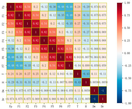
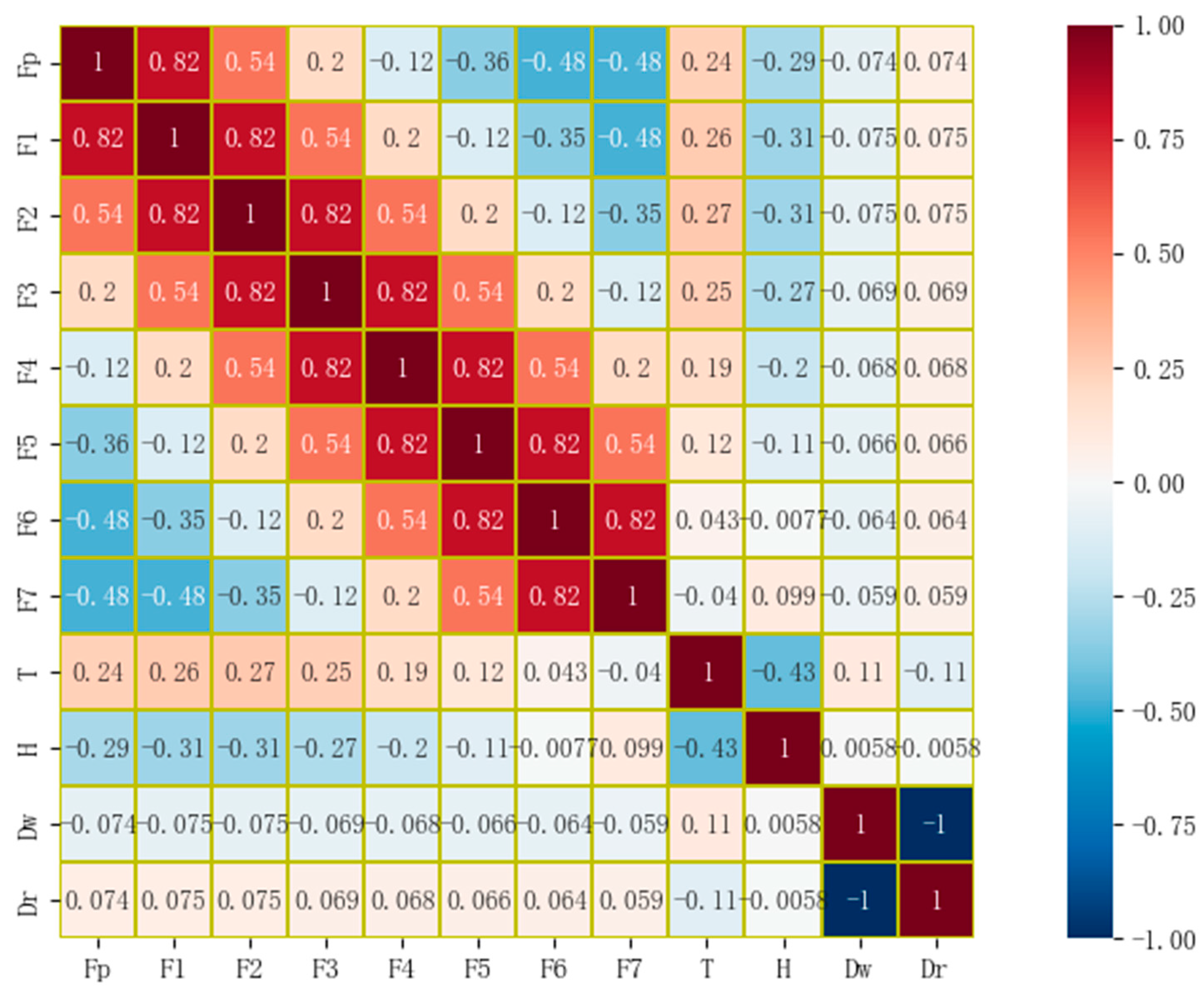
For the divided samples, the hourly water consumption values were calculated for different step lengths during the prediction period: F₁ for the first step, F₂ for the first two steps, F₃ for the first three steps, F₄ for the first four steps, F₅ for the first five steps, F₆ for the first six steps, and F₇ for the first seven steps. The correlation coefficients between temperature (T), humidity (H), and day type (weekday Dw, rest day Dr) and the hourly water consumption (Fp) during the prediction period were also calculated. These correlations were visualized in a heatmap of hourly water use correlations, as shown in Figure 7. The Pearson correlation coefficient (PCC) was used as the statistical method to assess the relationships between the variables, providing a clear visualization of the degree of correlation between each factor and hourly water consumption [26].

Figure 7. Pearson correlation coefficient heatmap.

The dataset was recorded for the period from 1 January 2023 to 30 June 2023, a total of 181 days (4337 hourly records). The data cover winter, spring, and summer seasons, capturing seasonal variations. As can be seen from Figure 7, if we want to predict the water consumption for the next hour, the input variables that will be selected are: F₁, F₂, F₅, F₆, F₇, temperature T, humidity H, weekdays Dw, and rest day Dr. The relevant data are shown in Table 2.

Table 2. Samples structure.

Time Series	Fp (m3)	F1 (m3)	F2 (m3)	F5 (m3)	F6 (m3)	F7 (m3)	Dw	Dr	T (℃)	H (%)
1 January 07:00–08:00	4	2	1	1	1	2	0	1	1.85	75.08
1 January 08:00–09:00	6	4	2	0	1	1	0	1	2.16	73.01
1 January 09:00–10:00	7	6	4	0	0	1	0	1	7.05	50.9
1 January 10:00–11:00	8	7	6	1	0	0	0	1	7.61	47.91
…	…	…	…	…	…	…	…	…	…	…
30 June 23:00–24:00	5	9	15	9	4	4	0	1	24.02	95.17

4. Results and Discussion

4.1. Model Initialization Parameter Setting

To determine the optimal hyperparameters of the prediction model, different algorithms were integrated into the BP neural network. For the PSO-GWO-BP model, the BP neural network structure was set as follows: input layer with nine neurons (corresponding to the nine selected input features: F₁, F₂, F₅, F₆, F₇, temperature T, humidity H, weekday Dw, and rest day Dr), one hidden layer with 10 neurons, and an output layer with one neuron (the predicted hourly water consumption). For the hybrid optimization, the maximum number of iterations was 200. The PSO parameters were: cognitive and social learning factors C₁ = C₂ = 1.4945, and inertia weight ω = 0.7298. The GWO convergence factor was linearly decreased from 2 to 0 over the course of iterations. The convergence criterion was defined as either the maximum number of iterations (200) being reached, or the change in fitness value being less than 10⁻⁶ for 20 consecutive generations. The specific parameters of the models involved are shown in Table 1.

4.2. Model Training Effects

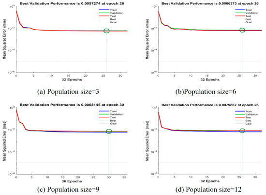
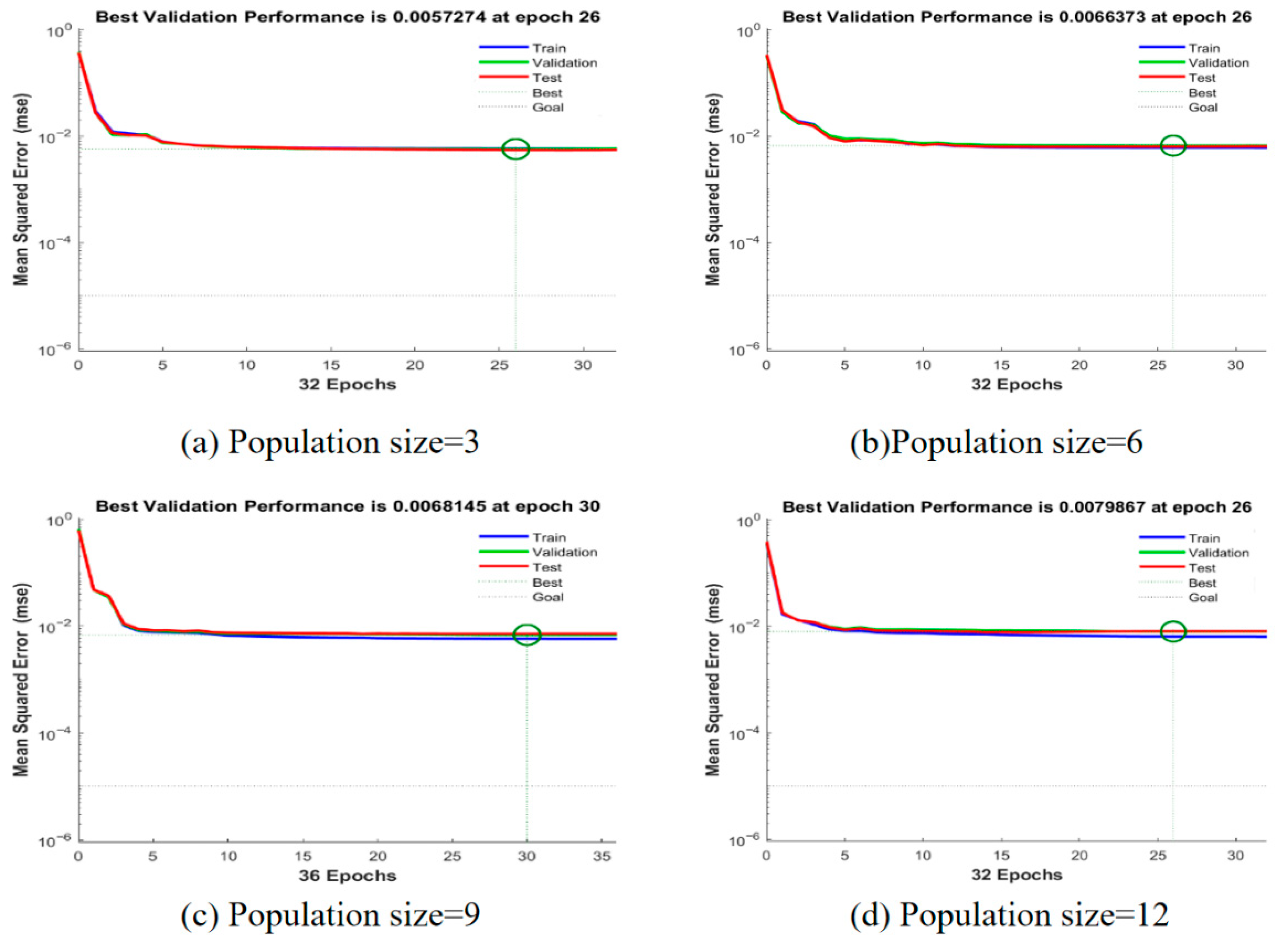
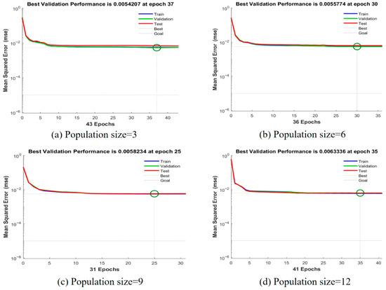
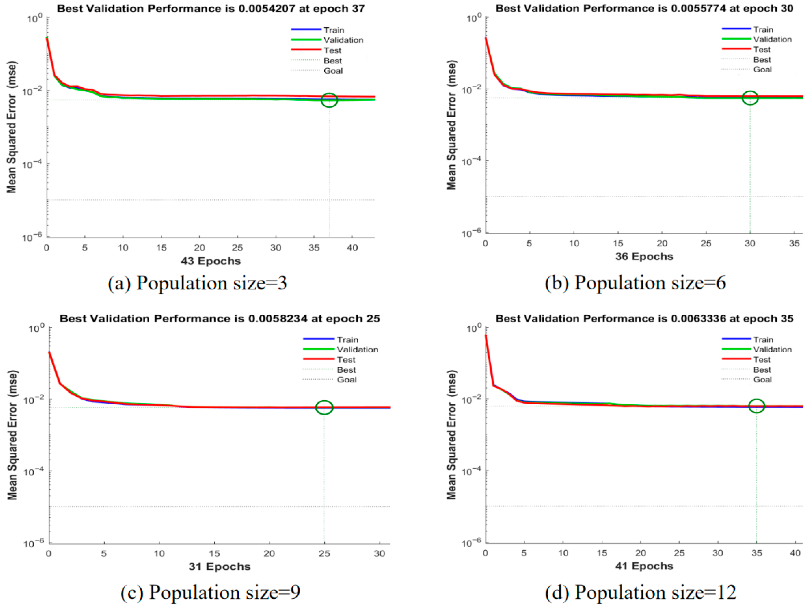
In each algorithm, the fitness function is used to evaluate the performance of each individual. In this study, the MSE between the predicted and actual values of water consumption was selected as the fitness function. The best fitness curve was obtained by running each algorithm three times for each of the different population sizes (3, 6, 9, and 12), based on 200 iterations. This is shown in Figure 8 and Figure 9.

Figure 8. Fitness curves of GWO-BP for different population sizes.

Figure 9. Fitness curves of PSO-GWO-BP for different population sizes.

Figure 8 shows that the fitness values of the GWO-BP model reached the lowest after 26 iterations when the population sizes were 3, 6, and 12. Among these, the best model performance occurred with a population size of 3, where the MSE reached 0.0057274. For a population size of 9, the fitness value resulted in a higher MSE of 0.0068145 after 30 iterations, indicating a poorer model performance. Figure 9 also shows that the model performance is optimal when the population size is 3. In comparison, the PSO-GWO-BP model achieved a minimum MSE of 0.0054207 after 37 iterations, requiring more iterations to reach convergence compared to the population sizes of 6, 9, and 12, which reached their minimum MSE values after 30, 25, and 35 iterations, respectively.

Due to the increased complexity of the model, the number of iterations required for the fitness value to reach its lowest point in the PSO-GWO-BP hybrid model is significantly higher compared to the GWO-BP model, which means the iterative performance of the model is improved. Therefore, the PSO-GWO algorithm is more effective in determining the hyperparameters of the BP neural network model.

4.3. Analysis of Model Prediction Results

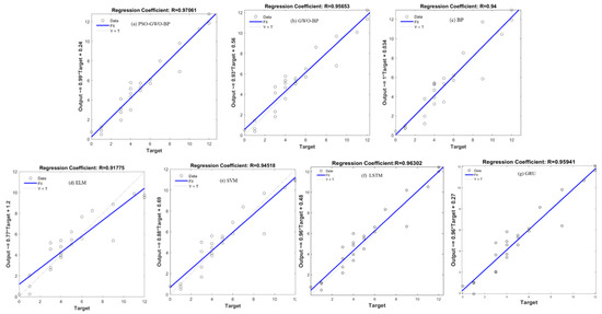
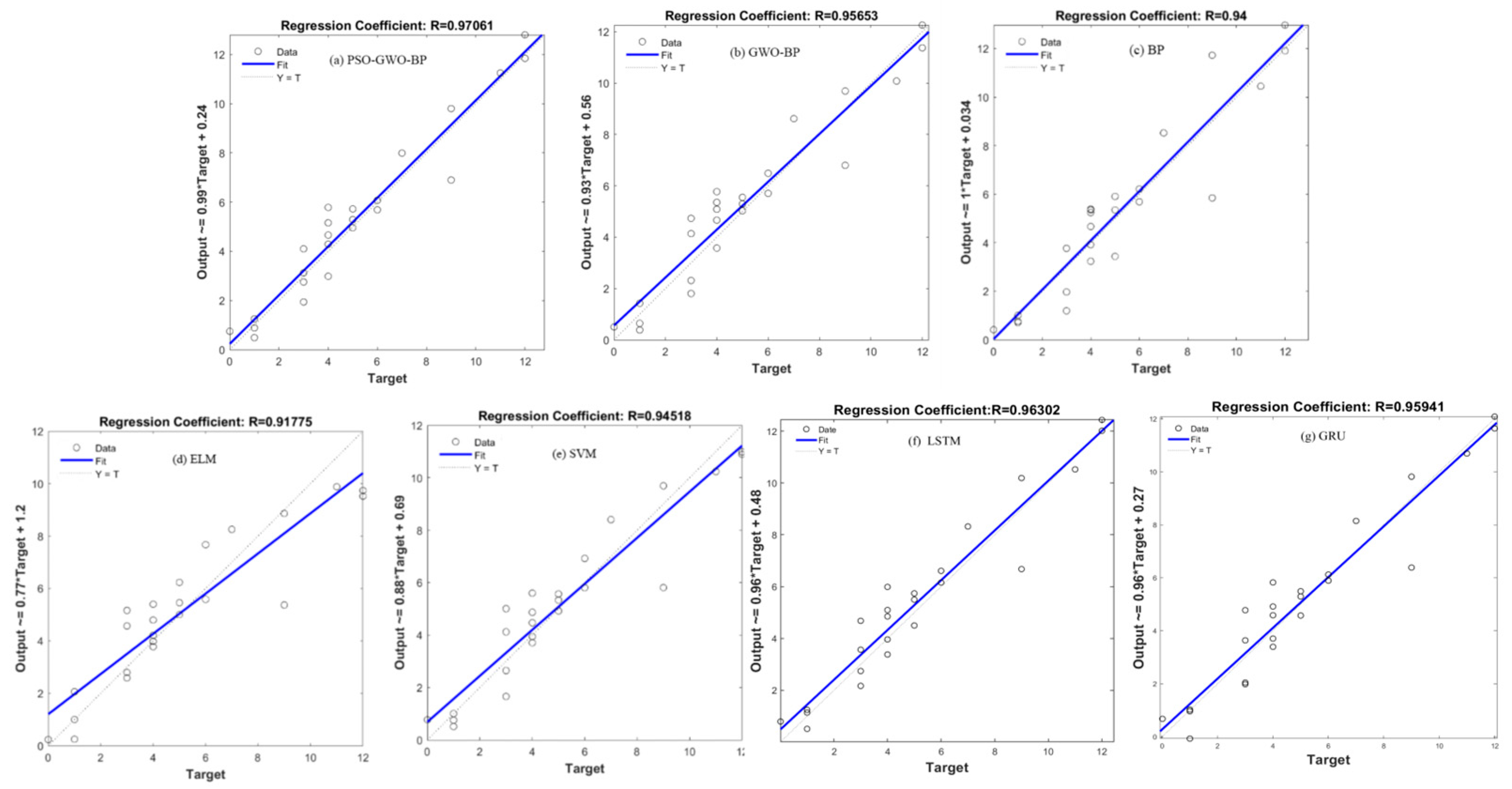
The regression coefficient (R) between the actual and predicted values is an important metric for evaluating the predictive performance of a model. A higher R-value indicates a stronger linear relationship between the actual and predicted values. The regression coefficients for the different models are presented in Figure 10.

Figure 10. Regression coefficients for different models.

A longitudinal comparison of the model prediction results reveals that, among the three BP neural networks, the PSO-GWO-BP model exhibits the best fit, with a regression coefficient of 0.97061. The GWO-BP model ranks second, with a regression coefficient of 0.95653, while the traditional BP model shows the weakest performance, with a regression coefficient of 0.94. After applying the hybrid improvement algorithm to optimize the BP neural network model, the regression coefficients of the hybrid-optimized BP model increased by 1.47% compared to the single GWO model, and by 3.26% compared to the traditional BP model. Cross-sectional comparison results show that the BP neural network model and the SVM model perform similarly in temporal water use prediction, while the ELM model is less effective in handling regression problems. The LSTM and GRU models achieve R values of 0.9630 and 0.9594, respectively, which are also lower than that of PSO-GWO-BP. For water use prediction, the PSO-GWO-BP model outperforms the ELM model by 5.76% and the SVM model by 2.69%, and outperforms the LSTM and GRU models by 0.79% and 1.17%, respectively. The GWO-BP model also performs better than the ELM and SVM models, suggesting that hybrid algorithms are more effective than single machine learning algorithms in prediction models.

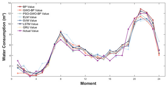
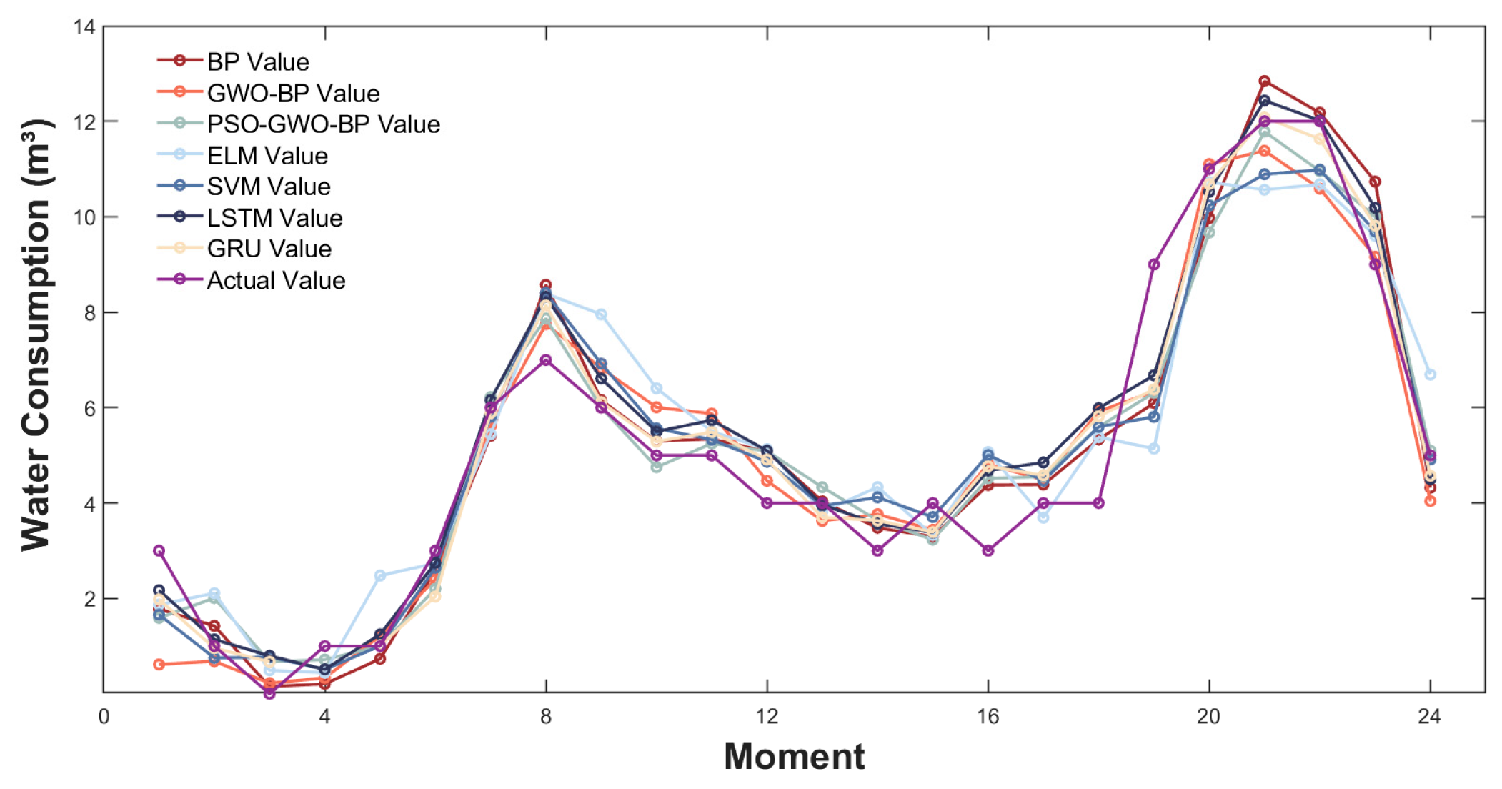
To visually illustrate the performance gap between the models, the predicted and actual water consumption curves for each model were plotted, as shown in Figure 11.

Figure 11. Plot of predicted versus actual water consumption curves for different models.

By examining the degree of curve fitting in the figure, it is evident that the three BP neural network models demonstrate superior fitting performance in predicting water consumption throughout the day. These models exhibit significantly higher prediction accuracy and greater robustness compared to the other two models. Nonetheless, among the BP neural network models, the GWO-BP model and the traditional BP model are less sensitive to the high and low peaks in water consumption than the PSO-GWO-BP model is. Both LSTM and GRU, owing to their strong computational capability for time series, also show good performance; however, their fitting degrees remain lower than that of the hybrid PSO-GWO-BP model.

To further evaluate model performance quantitatively, according to Section 2.4, multiple metrics—mean absolute error (MAE), mean squared error (MSE), mean absolute percentage error (MAPE), root mean square error (RMSE), Nash–Sutcliffe efficiency coefficient (NSE), regression coefficient (R), and coefficient of determination (R²)—are introduced to error analysis of the test set for the above models; the error values presented are the averages from 10 experiments for each model. The results of the evaluation metrics for the different models are shown in Table 3.

Table 3. Values of evaluation metrics for different models in the sample set.

Model	MAE	MSE	MAPE	R2	RMSE	NSE	R
PSO-GWO-BP	0.6305	0.7212	74.3938%	0.9421	0.8491	0.9006	0.9706
GWO-BP	0.7759	1.0350	190.9581%	0.9149	1.0173	0.8918	0.9565
BP	0.8193	1.4103	236.4509%	0.8836	1.1876	0.9058	0.94
ELM	1.1327	1.9585	465.2606%	0.8423	1.3994	0.8292	0.9178
SVM	0.8290	1.1885	338.3262%	0.8934	1.0903	0.8926	0.9452
LSTM	0.7440	0.8971	344.86%	0.9274	0.9471	0.9190	0.9630
GRU	0.7156	0.9015	294.42%	0.9205	0.9495	0.9186	0.9594

As presented in Table 3, the PSO-GWO-BP model achieves the best or competitive performance across nearly all evaluation metrics compared to GWO-BP, BP, ELM, SVM, LSTM, and GRU. Specifically, PSO-GWO-BP yields the lowest MAE (0.6305), MSE (0.7212), MAPE (74.3938%), and RMSE (0.8491), and the highest R (0.97061) and R² (0.9421) among all models. All models achieve NSE values above 0.82, demonstrating acceptable predictive capability. The PSO-GWO-BP model attains an NSE of 0.9006, which is slightly lower than those of LSTM (0.9190) and GRU (0.9186) but remains above 0.9, indicating very good model performance. More importantly, PSO-GWO-BP outperforms LSTM and GRU in terms of MAE, MSE, RMSE, and R, highlighting its superior ability to minimize absolute and squared errors. This suggests that while deep learning models may capture certain nonlinear patterns slightly better in terms of NSE, the proposed hybrid model provides more accurate point forecasts with smaller magnitude errors, which is practically more valuable for real-time water scheduling decisions. The lower MAPE of PSO-GWO-BP (74.39%) compared to LSTM (344.86%) and GRU (294.42%) further supports this conclusion. It should be noted that the high absolute MAPE values for all models are primarily due to the very low actual water consumption during off-peak hours (e.g., between 02:00 and 03:00 on the day of the test, when hourly water consumption is close to 0 m³). In such periods, even a small absolute error of 0.2 to 0.3 m³ can result in a very large relative error, which artificially inflates the MAPE. Nevertheless, the absolute errors are well within practical engineering tolerance for tank replenishment control, and the relative ranking of MAPE across models remains valid for comparison. These results confirm that the proposed hybrid model exhibits the highest prediction accuracy and the best robustness among all compared models, demonstrating the effectiveness of the tight PSO-GWO-BP coupling mechanism.

Table 4 presents the expanding window cross-validation results for the PSO-GWO-BP model. The proposed model achieves a mean MAPE of 74.52% with a standard deviation of 0.25%, a mean MAE of 0.6379 (SD = 0.0067), a mean MSE of 0.7292 (SD = 0.0082), a mean RMSE of 0.8539 (SD = 0.0048), a mean R of 0.9695 (SD = 0.0005), a mean R² of 0.9399 (SD = 0.0010), and a mean NSE of 0.8979 (SD = 0.0010). These values are very close to the single-day test results reported in Table 3 (MAPE = 74.39%, MAE = 0.6305, MSE = 0.7212, RMSE = 0.8491, R = 0.9706, R² = 0.9421, NSE = 0.9006), indicating that the high prediction accuracy is not coincidental but consistently reproducible across different time periods. The low standard deviations across folds further demonstrate the robustness of the PSO-GWO-BP model.

Table 4. Five-fold expanding window cross-validation results for the PSO-GWO-BP model.

Metric	1	2	3	4	5	Mean	Std
MAE	0.6281	0.6412	0.6398	0.6455	0.6349	0.6379	0.0067
MSE	0.7183	0.7325	0.7303	0.7401	0.7246	0.7292	0.0082
MAPE	74.2012	74.5247	74.6023	74.3881	74.8776	74.5188	0.2518
R2	0.9411	0.9399	0.9387	0.9406	0.9390	0.9399	0.0010
RMSE	0.8475	0.8559	0.8545	0.8603	0.8512	0.8539	0.0048
NSE	0.8992	0.8975	0.8968	0.8987	0.8971	0.8979	0.0010
R	0.9701	0.9695	0.9689	0.9698	0.9690	0.9695	0.0005

4.4. Water Scheduling Strategy Based on Model Prediction Results

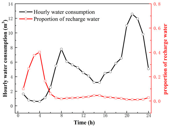
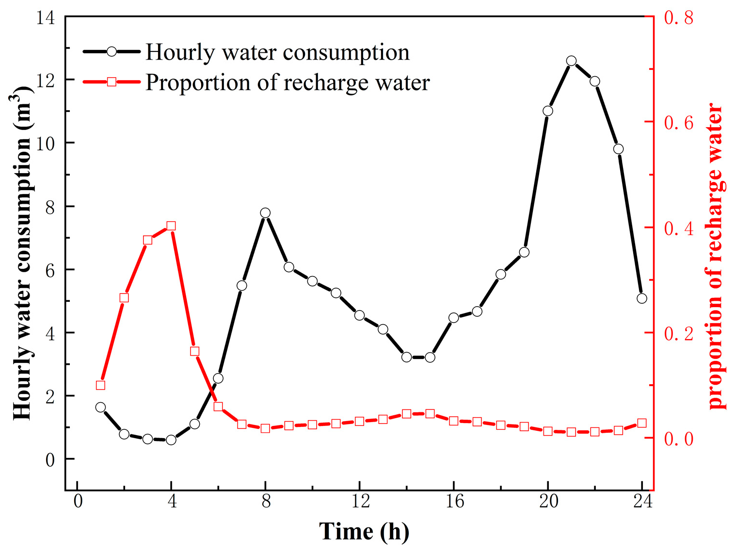
Based on the predicted hourly water demand derived from the proposed hybrid model, the replenishment water volume proportion can be dynamically adjusted by regulating the replenishment threshold level in the tanks. As shown in Figure 12, the predicted hourly water demand exhibits two peaks and two troughs within a single day: the morning peak occurs around 8:00 a.m., the evening peak around 9:00 p.m., and the troughs are observed in the early morning and afternoon. In response, the replenishment water volume proportion is inversely adjusted—increasing during low-demand periods to store water in the tanks and decreasing during peak-demand periods to prioritize the use of stored water. This strategy effectively flattens the peaks and valleys of water inflow [36]. By proactively raising the standby water level before peak-demand periods to allow increased inflow, and lowering it during peak hours to reduce inflow, this approach maximizes the utilization of stored water and minimizes the need for real-time pumping from the municipal network. This not only alleviates pressure on the municipal water distribution system but also reduces the operational energy consumption of building-level water supply equipment by avoiding frequent pump starts and high-load operation during peak hours. Such demand-responsive replenishment control aligns with the principles of green building operation and building energy efficiency, contributing to the intelligent and low-carbon management of secondary water supply systems.

Figure 12. Proportion of recharge corresponding to hourly water consumption prediction.

5. Conclusions

In this study, a hybrid prediction model was innovatively constructed by optimizing the traditional BP neural network with the GWO and PSO algorithms. At each iteration, the position of every gray wolf is updated using both the encircling mechanism of GWO and the velocity memory of PSO, enabling the social hierarchy of GWO and the individual historical information of PSO to work synergistically, thereby achieving faster convergence and higher prediction accuracy. The model’s performance was compared with that of individual machine learning methods, namely, ELM, SVM, LSTM, and GRU. This comparison was made using water consumption data from a single day in the study area. A time-series cross-validation scheme is further adopted to rigorously evaluate the model’s generalization ability and robustness. The effectiveness of the model’s predictions was verified and analyzed, and the feasibility of regulating the replenishment threshold level of water tanks to achieve a flexible water supply, based on the model’s predictions, was also explored. This approach offers a practical perspective for real-time water scheduling in building-level secondary water supply systems. The main conclusions are as follows:

(1)

Identification of key influencing factors: based on the study of water consumption patterns and the results of Pearson correlation analysis, the main factors influencing water consumption were identified: historical hourly water consumption data from 1, 2, 5, 6, and 7 h prior to the forecast period, along with temperature, humidity, and whether the day was a working day.

(2)

Development and performance evaluation of the hybrid prediction model: The proposed PSO-GWO-BP hybrid model achieved a predictive accuracy of 97.06%, outperforming standalone BP (94.00%), GWO-BP (95.65%), ELM (91.78%), SVM (94.52%), LSTM (96.30%), and GRU (95.94%). Based on the experimentally selected metrics, the hybrid prediction model outperformed the comparison models (BP, GWO-BP, ELM, SVM, LSTM, and GRU). Specifically, it reduced the MAE by 23.04%, 18.74%, 44.34%, 23.94%, 15.26%, and 11.89% respectively; the MSE by 48.86%, 30.32%, 63.18%, 39.32%, 19.61%, and 20.00% respectively; the RMSE by 28.51%, 16.53%, 39.33%, 22.12%, 10.35%, and 10.57% respectively; and the MAPE by 68.54%, 61.04%, 84.01%, 78.01%, 78.43%, and 74.33% respectively. These results demonstrate the superior performance of the hybrid model in hourly water consumption prediction, providing a reliable basis for real-time decision-making in building water supply systems.

(3)

Feasibility of prediction-driven water scheduling: The relationship between predicted hourly water consumption and replenishment proportion was analyzed. By pre-regulating the tank’s replenishment threshold level based on prediction results, the system enables real-time water supply scheduling. This demand-responsive strategy helps reduce unnecessary pump operations and energy consumption, contributing to the efficient and low-carbon operation of building-scale secondary water supply systems.

In summary, this study developed a high-precision water demand prediction model using PSO-GWO-BP and validated its advantages through comparative accuracy analysis. The findings support the integration of predictive intelligence into building water management, offering a viable pathway to enhance both water resource efficiency and energy performance in green building operations. Future research should address the current lack of long-term field validation, particularly energy data under different seasons and water usage patterns. We will collaborate with water utilities to deploy the model in real secondary water supply pumping stations for at least one year of online testing, collect actual energy saving data, and further optimize the threshold update strategy.

References

- Mannan, M.; Al-Ghamdi, S.G. Water Consumption and Environmental Impact of Multifamily Residential Buildings: A Life Cycle Assessment Study. Buildings 2022, 12, 48. [Google Scholar] [CrossRef] [Scilit]
- Eslamian, S.A.; Li, S.S.; Haghighat, F. A new multiple regression model for predictions of urban water use. Sustain. Cities Soc. 2016, 27, 419–429. [Google Scholar] [CrossRef] [Scilit]
- Jeandron, A.; Cumming, O.; Kapepula, L.; Cousens, S. Predicting quality and quantity of water used by urban households based on tap water service. npj Clean Water 2019, 2, 23. [Google Scholar] [CrossRef] [Scilit]
- Fullerton, T.M.; Ceballos, A.; Walke, A.G. Short-Term Forecasting Analysis for Municipal Water Demand. J. AWWA 2016, 108, E27–E38. [Google Scholar] [CrossRef] [Scilit]
- Yasar, A.; Bilgili, M.; Simsek, E. Water Demand Forecasting Based on Stepwise Multiple Nonlinear Regression Analysis. Arab. J. Sci. Eng. 2012, 37, 2333–2341. [Google Scholar] [CrossRef] [Scilit]
- Gagliardi, F.; Alvisi, S.; Kapelan, Z.; Franchini, M. A Probabilistic Short-Term Water Demand Forecasting Model Based on the Markov Chain. Water 2017, 9, 507. [Google Scholar] [CrossRef] [Scilit]
- Gharabaghi, S.; Stahl, E.; Bonakdari, H. Integrated nonlinear daily water demand forecast model (case study: City of Guelph, Canada). J. Hydrol. 2019, 579, 124182. [Google Scholar] [CrossRef] [Scilit]
- Shan, S.; Ni, H.; Chen, G.; Lin, X.; Li, J. A Machine Learning Framework for Enhancing Short-Term Water Demand Forecasting Using Attention-BiLSTM Networks Integrated with XGBoost Residual Correction. Water 2023, 15, 3605. [Google Scholar] [CrossRef] [Scilit]
- Bárdossy, G.; Halász, G.; Winter, J. Prognosis of urban water consumption using hybrid fuzzy algorithms. J. Water Supply Res. Technol.-AQUA 2009, 58, 203–211. [Google Scholar] [CrossRef] [Scilit]
- Smolak, K.; Kasieczka, B.; Fialkiewicz, W.; Rohm, W.; Siła-Nowicka, K.; Kopańczyk, K. Applying human mobility and water consumption data for short-term water demand forecasting using classical and machine learning models. Urban Water J. 2020, 17, 32–42. [Google Scholar] [CrossRef] [Scilit]
- Yu, K.; Liu, L.; Chen, Z. An Improved Slime Mould Algorithm for Demand Estimation of Urban Water Resources. Mathematics 2021, 9, 1316. [Google Scholar] [CrossRef] [Scilit]
- Herrera, M.; Torgo, L.; Izquierdo, J.; Pérez-García, R. Predictive models for forecasting hourly urban water demand. J. Hydrol. 2010, 387, 141–150. [Google Scholar] [CrossRef] [Scilit]
- Asgarkhani, N.; Kazemi, F.; Jankowski, R.; Formisano, A.J.R.E.; Safety, S. Dynamic ensemble-learning model for seismic risk assessment of masonry infilled steel structures incorporating soil-foundation-structure interaction. Reliab. Eng. Syst. Saf. 2026, 267, 111839. [Google Scholar] [CrossRef] [Scilit]
- Singh, M.K.; Kekatos, V. Optimal Scheduling of Water Distribution Systems. IEEE Trans. Control Netw. Syst. 2020, 7, 711–723. [Google Scholar] [CrossRef] [Scilit]
- Xia, H.; Wang, C.; Sun, J.; Lei, X.; Wang, H. Multi-scale closed-loop coupled real-time water quantity optimization scheduling of cascade pumping station in water supply canal systems. J. Hydrol. 2024, 641, 131802. [Google Scholar] [CrossRef] [Scilit]
- Yuan, W.; Yu, X.; Su, C.; Yan, D.; Wu, Z. A Multi-Timescale Integrated Operation Model for Balancing Power Generation, Ecology, and Water Supply of Reservoir Operation. Energies 2020, 14, 47. [Google Scholar] [CrossRef] [Scilit]
- Dini, M.; Hemmati, M.; Hashemi, S. Optimal Operational Scheduling of Pumps to Improve the Performance of Water Distribution Networks. Water Resour. Manag. 2022, 36, 417–432. [Google Scholar] [CrossRef] [Scilit]
- Lyu, J.; Zhang, J. BP neural network prediction model for suicide attempt among Chinese rural residents. J. Affect. Disord. 2019, 246, 465–473. [Google Scholar] [CrossRef] [Scilit]
- Liu, X.; Zhou, G.; Zhou, Y.; Luo, Q. Functional extreme learning machine. Front. Comput. Neurosci. 2023, 17, 1209372. [Google Scholar] [CrossRef] [Scilit]
- Kashef, R. A boosted SVM classifier trained by incremental learning and decremental unlearning approach. Expert Syst. Appl. 2021, 167, 114154. [Google Scholar] [CrossRef] [Scilit]
- Wang, D.; Tan, D.; Liu, L. Particle swarm optimization algorithm: An overview. Soft Comput. 2017, 22, 387–408. [Google Scholar] [CrossRef] [Scilit]
- Liu, Y.; As’arry, A.; Hassan, M.K.; Hairuddin, A.A.; Mohamad, H. Review of the grey wolf optimization algorithm: Variants and applications. Neural Comput. Appl. 2023, 36, 2713–2735. [Google Scholar] [CrossRef] [Scilit]
- Liu, H. Optimal selection of control parameters for automatic machining based on BP neural network. Energy Rep. 2022, 8, 7016–7024. [Google Scholar] [CrossRef] [Scilit]
- Kumar, R.; Singh, L.; Tiwari, R. Path planning for the autonomous robots using modified grey wolf optimization approach. J. Intell. Fuzzy Syst. 2021, 40, 9453–9470. [Google Scholar] [CrossRef] [Scilit]
- Hou, K.; Guo, M.; Li, X.; Zhang, H. Research on Optimization of GWO-BP Model for Cloud Server Load Prediction. IEEE Access 2021, 9, 162581–162589. [Google Scholar] [CrossRef] [Scilit]
- Afyouni, S.; Smith, S.M.; Nichols, T.E. Effective degrees of freedom of the Pearson’s correlation coefficient under autocorrelation. NeuroImage 2019, 199, 609–625. [Google Scholar] [CrossRef] [Scilit]
- Cui, L.; Tao, Y.; Deng, J.; Liu, X.; Xu, D.; Tang, G. BBO-BPNN and AMPSO-BPNN for multiple-criteria inventory classification. Expert Syst. Appl. 2021, 175, 114842. [Google Scholar] [CrossRef] [Scilit]
- Liu, P.; Zhang, W. A Fault Diagnosis Intelligent Algorithm Based on Improved BP Neural Network. Int. J. Pattern Recognit. Artif. Intell. 2019, 33, 1959028. [Google Scholar] [CrossRef] [Scilit]
- Liu, Y.; Shao, Q.; Liu, Y.; Yang, D. An interval neural network-based Caputo fractional-order extreme learning machine applied to classification. Appl. Soft Comput. 2024, 167, 112310. [Google Scholar] [CrossRef] [Scilit]
- Jin, Y.; Lee, S.M. Sampled-Data State Estimation for LSTM. IEEE Trans. Neural Netw. Learn. Syst. 2025, 36, 2300–2313. [Google Scholar] [CrossRef] [Scilit]
- Yang, M.; Li, M.; Li, G. On memory-augmented gated recurrent unit network. Int. J. Forecast. 2025, 41, 844–858. [Google Scholar] [CrossRef] [Scilit]
- Divasón, J.; Ceniceros, J.F.; Sanz-Garcia, A.; Pernia-Espinoza, A.; Martinez-de-Pison, F.J. PSO-PARSIMONY: A method for finding parsimonious and accurate machine learning models with particle swarm optimization. Application for predicting force–displacement curves in T-stub steel connections. Neurocomputing 2023, 548, 126414. [Google Scholar] [CrossRef] [Scilit]
- Hou, Y.; Gao, H.; Wang, Z.; Du, C. Improved Grey Wolf Optimization Algorithm and Application. Sensors 2022, 22, 3810. [Google Scholar] [CrossRef] [Scilit]
- Dawson, C.W.; Abrahart, R.J.; See, L.M. HydroTest: A web-based toolbox of evaluation metrics for the standardised assessment of hydrological forecasts. Environ. Model. Softw. 2007, 22, 1034–1052. [Google Scholar] [CrossRef] [Scilit]
- Li, H.; Li, S.; Tang, W.; Yang, Y.; Zhao, J.; Xia, S.; Zhang, W.; Wang, H. Influence of secondary water supply systems on microbial community structure and opportunistic pathogen gene markers. Water Res. 2018, 136, 160–168. [Google Scholar] [CrossRef] [Scilit]
- Wang, J.; Deng, B.; Jiang, S.; Deng, Z.; Wang, W.; Chen, G.; Liu, L. Optimizing Control of Secondary Water Supply Tanks for Demand Peak Staggering. Water Resour. Manag. 2024, 38, 4123–4136. [Google Scholar] [CrossRef] [Scilit]
Disclaimer/Publisher’s Note: The statements, opinions and data contained in all publications are solely those of the individual author(s) and contributor(s) and not of MDPI and/or the editor(s). MDPI and/or the editor(s) disclaim responsibility for any injury to people or property resulting from any ideas, methods, instructions or products referred to in the content. |
© 2026 by the authors. Licensee MDPI, Basel, Switzerland. This article is an open access article distributed under the terms and conditions of the Creative Commons Attribution (CC BY) license.