Research on the Distribution and Prediction of Wind Pressure on Airport Terminal Glass Curtain Walls Based on Wind Tunnel Testing and Numerical Simulation

Abstract

Glass curtain walls are widely used in the enclosure structure of airport terminals due to their advantages of lightweight and beautiful appearance, good lighting, and easy installation. However, coastal areas are constantly affected by typhoons, and under the influence of strong winds, complex pressure distributions are generated on the surface of curtain walls. Therefore, studying the wind pressure distribution characteristics of glass curtain walls is crucial for the structural safety and durability of coastal airport terminals. Based on this, accurately predicting wind pressure distribution not only helps to improve the design safety of airport terminals but also effectively prevents potential damage under strong wind conditions. To achieve effective prediction of wind pressure on glass curtain walls, this paper adopts a combination of wind tunnel tests and neural network prediction models. Real wind pressure coefficient data is obtained through wind tunnel tests, and a CNN–Transformer combination model is proposed to predict wind pressure coefficients. The results show that the prediction accuracy of the combined model is higher than that of the CNN and Transformer single models. MAE is optimized by 0.04~0.10 compared with the former and 0.16~0.34 compared with the latter; RMSE has been optimized by 0.02–0.10 and 0.30–0.34, respectively. This article can provide reference for the prediction research of wind pressure on the surface of glass curtain walls in airport terminals.

1. Introduction

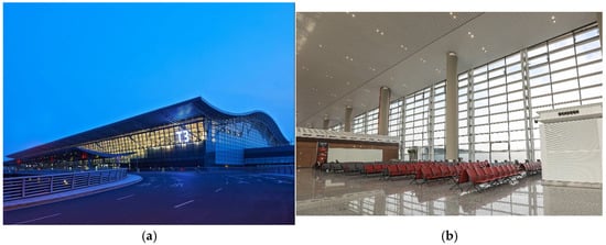
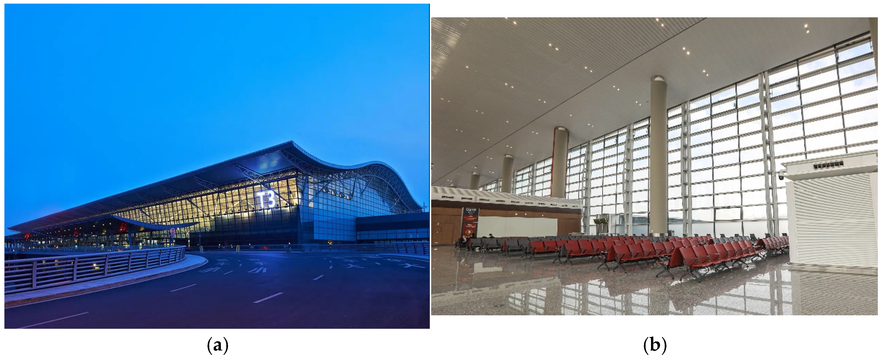
The terminal building serves as a critical transportation hub and represents the most wind-sensitive structure in airport complexes. Contemporary architectural designs increasingly favor glass curtain walls as the primary envelope system for terminal buildings, owing to their aesthetic appeal and superior daylighting performance. However, these façade elements are directly exposed to wind loads, as shown in Figure 1, making them particularly vulnerable in coastal regions prone to typhoon activity. Extreme wind conditions can substantially alter pressure distributions across curtain wall surfaces, potentially compromising both structural integrity and occupant comfort. Consequently, investigating typhoon-induced wind pressure patterns on terminal building enclosures and developing reliable prediction methodologies carries substantial engineering importance.

Figure 1. Schematic diagram of the glass curtain wall of the coastal airport terminal: (a) outside the glass wall; (b) inside the glass wall.

In wind-engineering-related research, wind tunnel testing is an important tool to study wind pressure distribution. Gerhardt et al. [1] conducted wind tunnel experiments on the wind load distribution of curtain walls with openings in buildings and systematically studied the key parameters of double curtain wall design such as the relative external dimensions of buildings. Gomes et al. [2] studied the effect of the outer curtain wall on the wind pressure distribution of the inner curtain wall of the monolithic double curtain wall system for high-rise buildings with rectangular cross-sections by means of wind tunnel experiments. Kawai et al. [3] investigated the distribution pattern of the mean and extreme values of the wind pressure of the window box type double curtain wall system and concluded that whether the inner curtain wall opens or closes a window has a greater influence on the wind pressure distribution of the inner and outer curtain walls. Through comprehensive wind tunnel experiments, Kim et al. [4] examined how extensive adjacent building clusters affect wind load characteristics on standard low-rise structures. In a related study focusing on architectural aerodynamics, Chen and Li [5] conducted experimental investigations on Guangzhou’s exhibition center, analyzing pressure distribution patterns across both interior and exterior curtain wall surfaces of the long-span roof system. Liu et al. [6] found that the distribution of wind pressure coefficients of rectangular buildings with different plan sizes varied greatly by means of wind tunnel tests. In the same year, Sun et al. [7] investigated the effects of wind direction, span, eave height, and terrain roughness on the wind pressure distribution of a long-span roof through wind tunnel experiments. Wu et al. [8] investigated the effects of different wind angles on the pulsation characteristics of the wind pressure of a long-span roof structure under sealed and open conditions through wind tunnel experiments. Through systematic wind tunnel investigations, Yang et al. [9] examined how varying wind incidence angles influence the fluctuating pressure patterns on large-span curved roof structures.

Among the many prediction methods, prediction research combined with neural network models is an important direction, which has been widely applied in various fields. The use of neural network models for prediction has a high degree of flexibility and adaptability and can better deal with a large number of complex data; in addition, its powerful nonlinear modeling ability makes it able to effectively capture the potential patterns in complex data and thus improve the accuracy of prediction. Wind pressure prediction has an important application value in the field of engineering, and considering the impact of wind pressure can improve the safety and durability of the glass curtain wall structure of a terminal building. For the prediction of wind pressure, many scholars have constructed neural network models to achieve the purpose. Tian et al. [10] proposed a deep neural network-based scale-modeled low-rise cable-roofed building to predict surface mean and peak wind pressure coefficients. The prediction method improved the accuracy of the prediction. Kang et al. [11] proposed a back-propagation neural network combined with the proper orthogonal decomposition (POD) method to predict the roof surface wind pressures, and the prediction results were generally satisfactory. Vigneshwaran et al. [12] used an ANN to predict the wind-induced pressures on the planar shaped building of the Pentagon. The results obtained were in good agreement. Ding et al. [13] proposed two new methods, genetic algorithm neural network and Bayesian optimization neural network, for wind pressure prediction of low-rise buildings. Chen et al. [14] predicted the wind pressure on the surface of high-rise buildings using a wavelet neural network and achieved satisfactory prediction results. Wu et al. [15] constructed a new model for wind pressure prediction of low-rise buildings based on a deep convolutional neural network (CNN), which has a higher prediction accuracy compared with other models. Huang et al. [16] proposed a new method combining POD and machine learning for the prediction of the time series of wind pressures of models of ultra-high-rise buildings in a wind tunnel test.

In summary, this article takes the typical glass curtain wall of airport terminals in coastal areas as the research object. Based on wind tunnel tests, the wind pressure distribution characteristics of glass curtain walls are studied, and a combination prediction model of CNN–Transformer is proposed to predict the wind pressure coefficient. The findings of this study can inform the design and construction of airport terminal glass curtain walls and also provide a foundation for future research on the rapid prediction of wind pressure coefficients.

2. Methodologies

2.1. Data Processing

Wind tunnel experiments typically provide measured data in terms of dimensionless pressure coefficients. To analyze the aerodynamic loading on glass curtain walls, the recorded surface pressures must be normalized to derive their corresponding coefficient time series. The normalization procedure follows the computational approach detailed below:

$$C_{pi}(t_j)=[P_i(t_j)-P_{\infty }]/0.5\rho {U_0}^2$$

(1)

In the formula, $C_{pi}(t_j)$ represents the dimensionless pressure coefficient for the i-th measurement location at time instant t; $P_i$ denotes the instantaneous pressure reading acquired from the scanning valve system; $P_{\infty }$ corresponds to the mean static pressure measured at the reference position; $U_0$ signifies the freestream velocity at the model’s peak elevation; and $\rho$ indicates the ambient air density.

Based on the above wind pressure coefficients, the average wind pressure coefficient and fluctuating wind pressure coefficient of each measuring point on the curtain wall surface can be calculated using Equations (2) and (3), as follows:

$${\overline{C}}_{pi}={\displaystyle \frac{{\displaystyle \sum _{j=1}^N{C}_{pi}(t_j)}}{M}}$$

(2)

$$C_{pri}=\sqrt{{\displaystyle \frac{1}{M}}{\displaystyle \sum _{j=1}^N{[C_{pi}(t_j)-{\overline{C}}_{pi}]}^2}}$$

(3)

In the formula, ${\overline{C}}_{pi}$ represents the mean value of the wind pressure coefficient; $C_{pri}$ denotes the fluctuating component of the wind pressure coefficient; and M indicates the complete set of sampling locations for the measurement point.

2.2. CNN Model

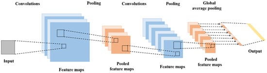
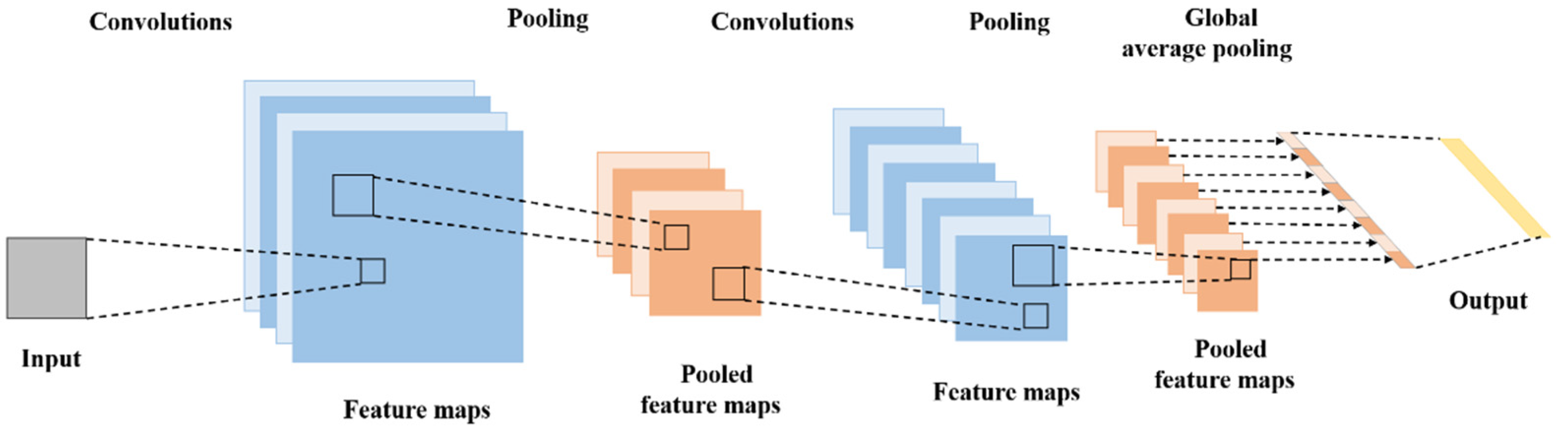
CNN is a deep learning model whose foundations date back to the 1980s but have really taken off since 2012 and are widely used in a number of domains. The architecture of CNN consists of three basic components: a convolutional layer, a pooling layer, and a fully connected layer. Figure 2 illustrates the architectural design.

Figure 2. Structure of CNN mode.

The convolutional layer is the core part of the CNN, which extracts features from the input image using convolutional operations. This layer uses multiple filters that glide over the image to generate feature maps that capture important information such as edges, texture, etc., in the image. The role of the pooling layer is to downsample the feature maps. Maximum or average pooling operations reduce the dimensionality of the features, which reduces the computational burden and improves the robustness of the model. This step helps retain important features while reducing sensitivity to small variations. The fully connected layer integrates the features after convolution and pooling to output the final classification result. In many applications, the final layer is typically combined with an activation function to transform the output into a probability distribution for multi-class classification tasks.

In terms of prediction, CNNs excel at image and time series tasks thanks to their powerful feature extraction capabilities and the way neurons work to significantly reduce model parameters through local connectivity and weight sharing, making training more efficient.

2.3. Transformer Model

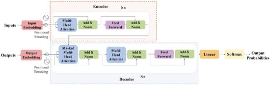
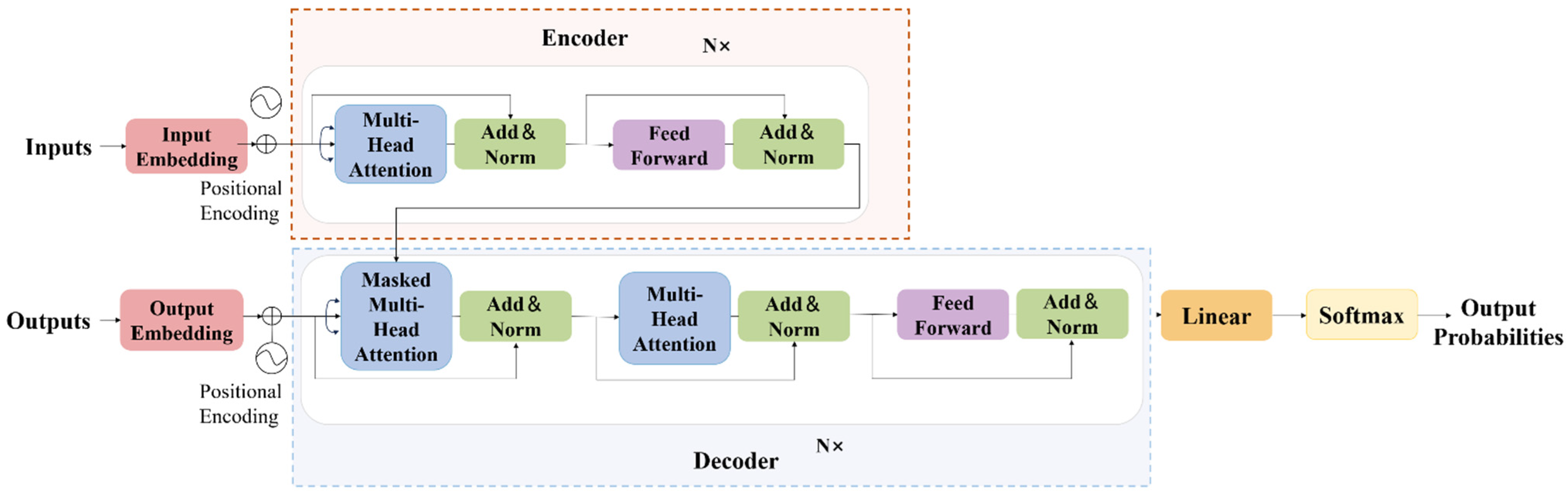
The Transformer architecture represents an advanced deep learning framework that employs self-attention mechanisms, initially introduced by Google Brain researchers in 2017. This innovative approach has found extensive applications across various domains, including NLP and image analysis. In contrast to conventional RNNs, the Transformer architecture demonstrates superior parallel computation efficiency and effectively addresses limitations associated with long-range dependencies in sequential data.

Structurally, the model incorporates two principal modules: an encoding component and a decoding component. The encoder processes input sequences to generate contextual representations, whereas the decoder utilizes these representations to produce the desired output. Each encoding layer integrates two fundamental operations: a multi-head attention mechanism that examines interdependencies among input elements and a position-wise feedforward network. The multi-head design permits simultaneous learning across multiple representation subspaces, while the self-attention operation computes relevance scores between sequence elements to determine optimal feature combinations.

The Transformer’s principal strengths are its capabilities for parallel processing and long-range dependency modeling. Its self-attention mechanism enables the model to adaptively focus on different parts of the sequence when processing input data. The introduction of the self-attention mechanism’s parallel processing capability, flexible input processing, and powerful feature learning capabilities facilitate the effective management of complex and dynamically changing data as it is received. As the model continues to be refined, the Transformer is seeing further applications, and it is also demonstrating excellent performance in prediction tasks, as illustrated in Figure 3.

Figure 3. Structure of Transformer mode.

3. Wind Tunnel Testing

3.1. Experimental Fundamentals

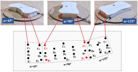
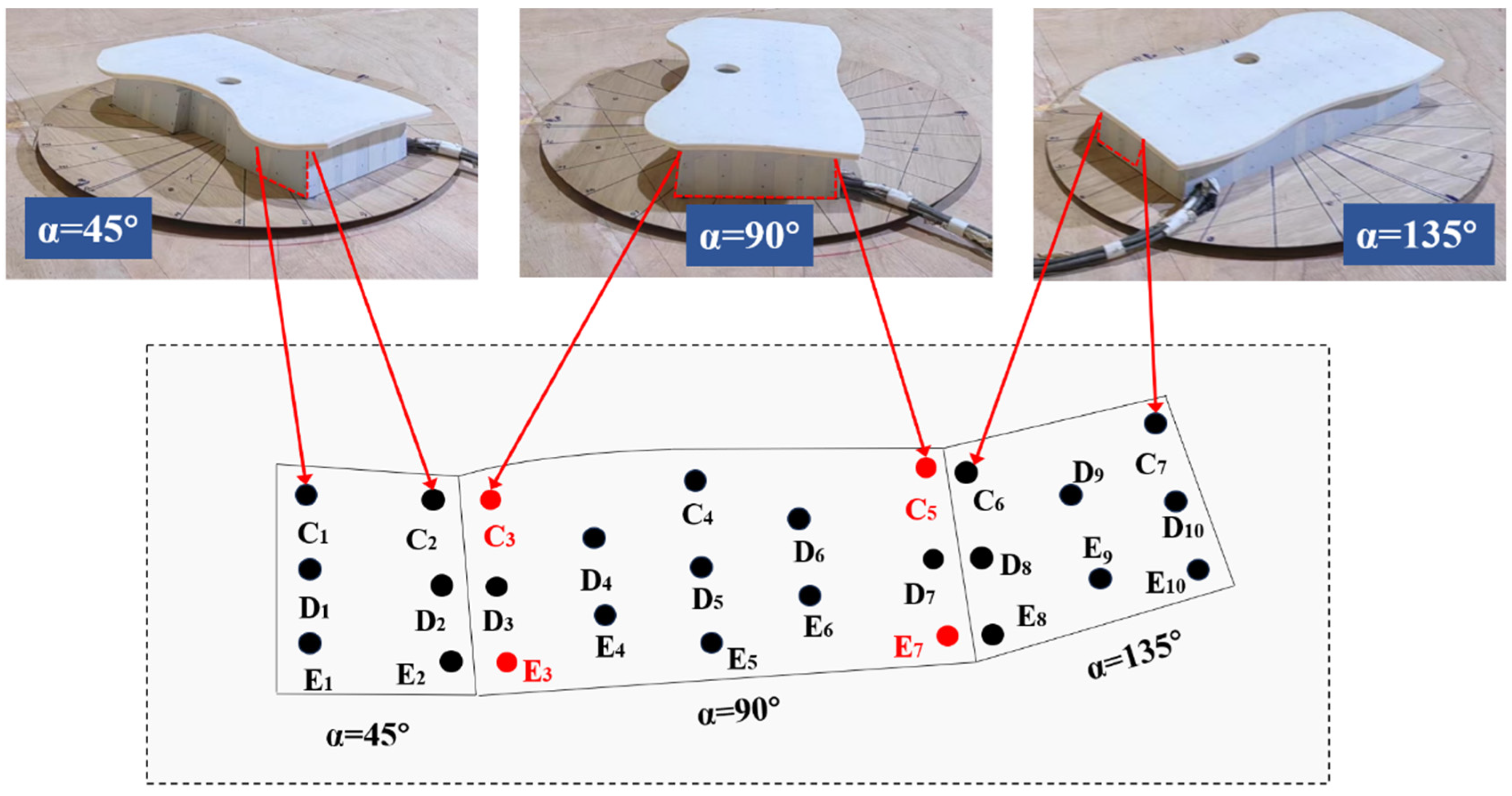
In this study, the glass curtain wall of the identified coastal airport terminal building serves as the research object for conducting wind tunnel tests. The dimensions of the airport terminal building adopted for this study were 102 m × 53 m × 60 m (length × width × height). A model for experimental purposes was constructed at a scale of 1:200, in accordance with the design and construction data, in order to meet the requirements of the wind tunnel test of the airport terminal building. Once the model was complete, it was placed on the base with the angle data clearly labeled for the experiments. The photographs of the test model are presented in Figure 4.

Figure 4. Schematic diagram of airport terminal model and glass curtain wall surface measurement points.

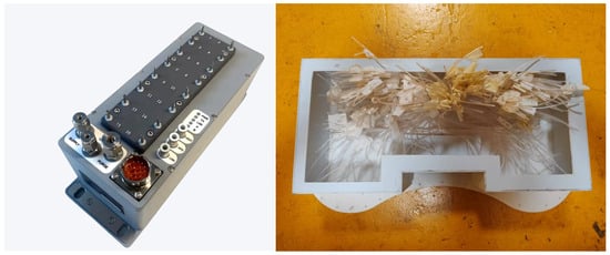
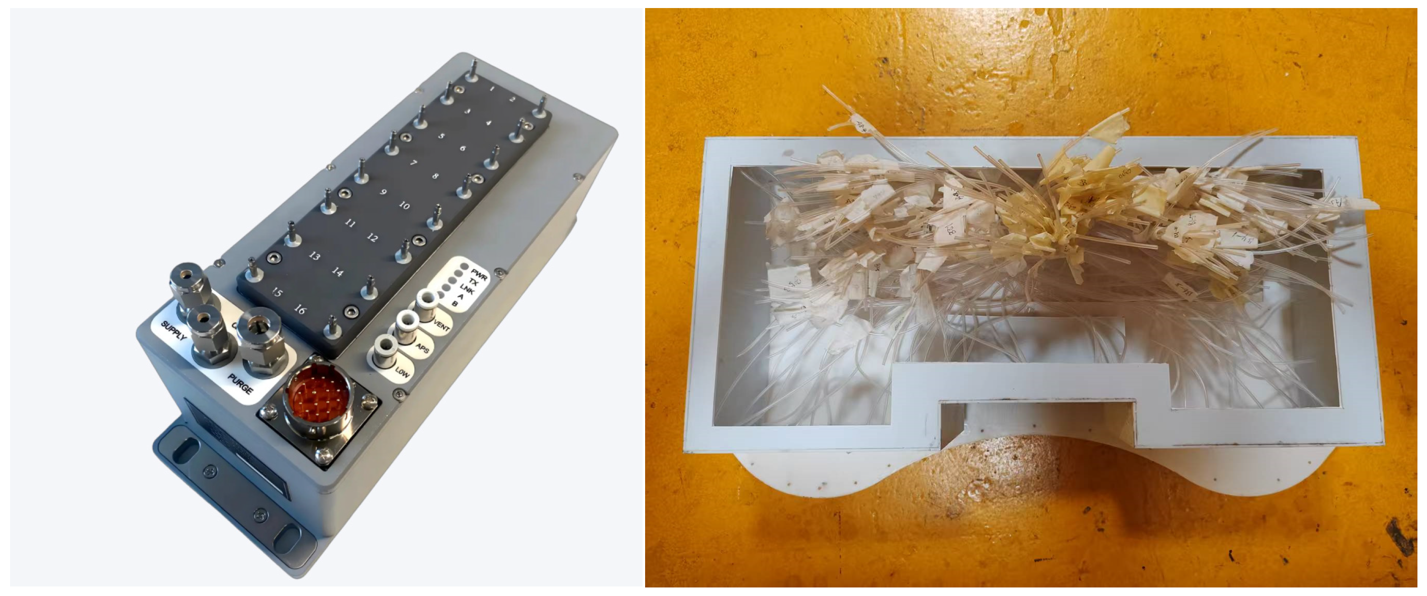
The experiment was conducted in the wind tunnel of the XNJD-1 wind tunnel facility at Southwest Jiaotong University. The cross-sectional area of the structure is 3.0 m (height) × 3.6 m (width). The test section was equipped with Scanivalve ZOC33 (Scanivalve Corporation, Washington, DC, USA) pressure scanners, which were used to measure the pressure on the surface of the glass curtain wall. These were connected to a Scanivalve DSM4000 (Scanivalve Corporation, Washington, DC, USA), which ensured simultaneous, timed pressure acquisition. Each scanner is equipped with 64 channels, as shown in Figure 5. The pressure measurement ports were 1 mm in diameter. All scanning devices were securely mounted within the model to ensure that the length of the tubing did not exceed 0.2 m. Digital filters were developed and employed to maintain signal integrity. For each test, the sampling frequency and time were set to 256 Hz and 60 s, respectively. The blocking rate was less than 5%. In order to obtain accurate wind pressure distribution characteristics, the pressure data were collected by placing measurement points in a symmetrical arrangement on the surface of the glass curtain wall, with a similar configuration on either side of the airport terminal building. In order to obtain a comprehensive understanding of the wind pressure distribution characteristics, the wind angle was gradually transitioned from 0° to 180° in 15° steps, forming 12 subconditions for each test condition.

Figure 5. Scanivalve DSM4000.

3.2. Simulation of Wind Environment

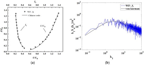
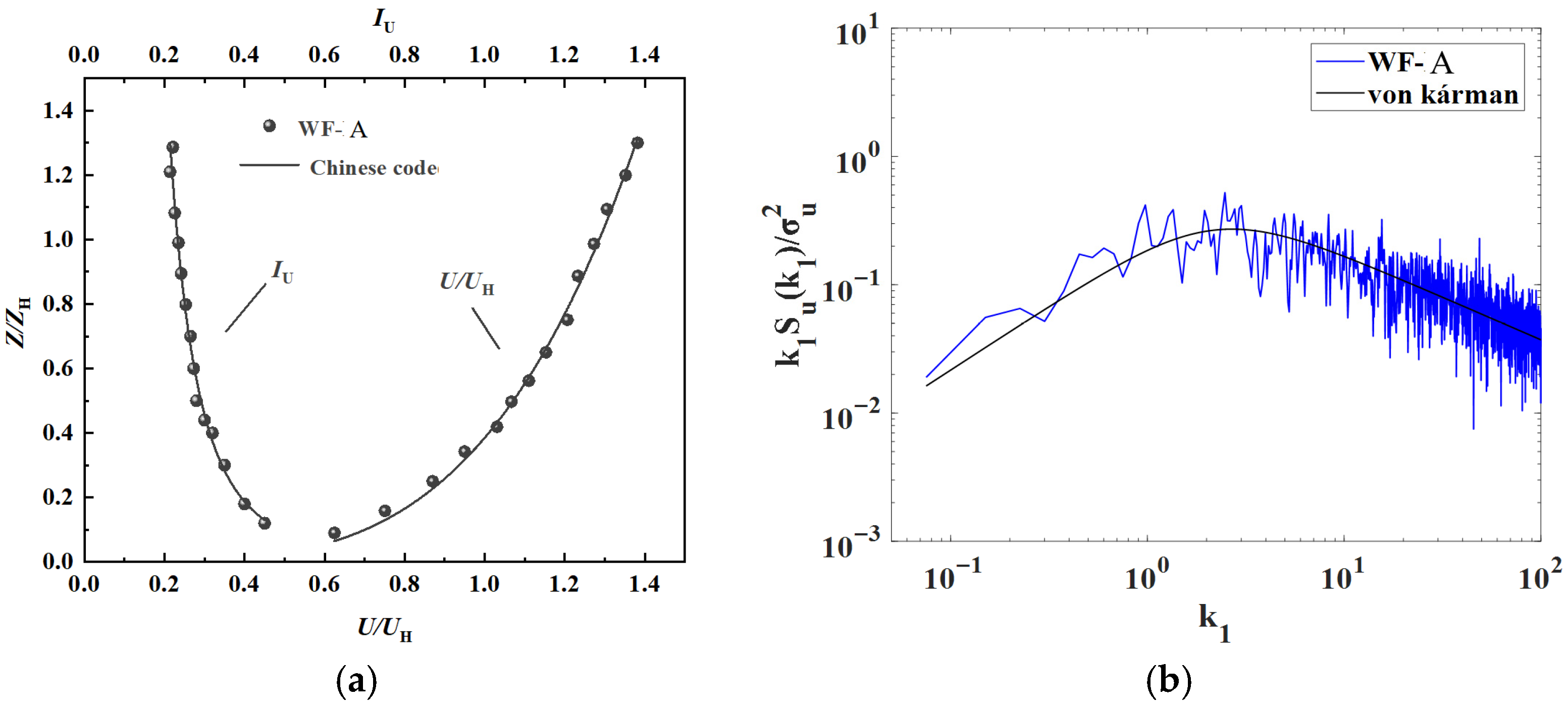
In accordance with the Chinese specification (GB50009-2012) [17], simulated coastal typhoon environments are classified as Level A. Initially, preliminary tests were conducted to ascertain the consistency of the prepared environments with the requirements of Class A. The data collected were plotted in Figure 6 for subsequent analysis. Experimental measurements of both mean wind velocity distributions and turbulence intensity characteristics exhibit close agreement with established reference values. Furthermore, spectral analysis confirms that the fluctuating wind velocity components follow the theoretical von Kármán distribution. These findings collectively validate that the numerically generated wind field satisfies all prescribed simulation criteria.

Figure 6. Class A atmospheric boundary layer simulated by wind tunnel tests: (a) mean velocity and intensity and (b) wind spectrum. Note: U = the wind speed; Z = the height; I_U = the turbulence intensity; U_H = the model reference point wind speed; Z_H stands for the model reference point height; k₁ = the index of refraction.

4. Results and Discussion

4.1. Mean and Fluctuating Wind Pressure Coefficients

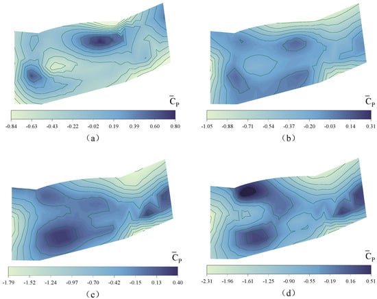
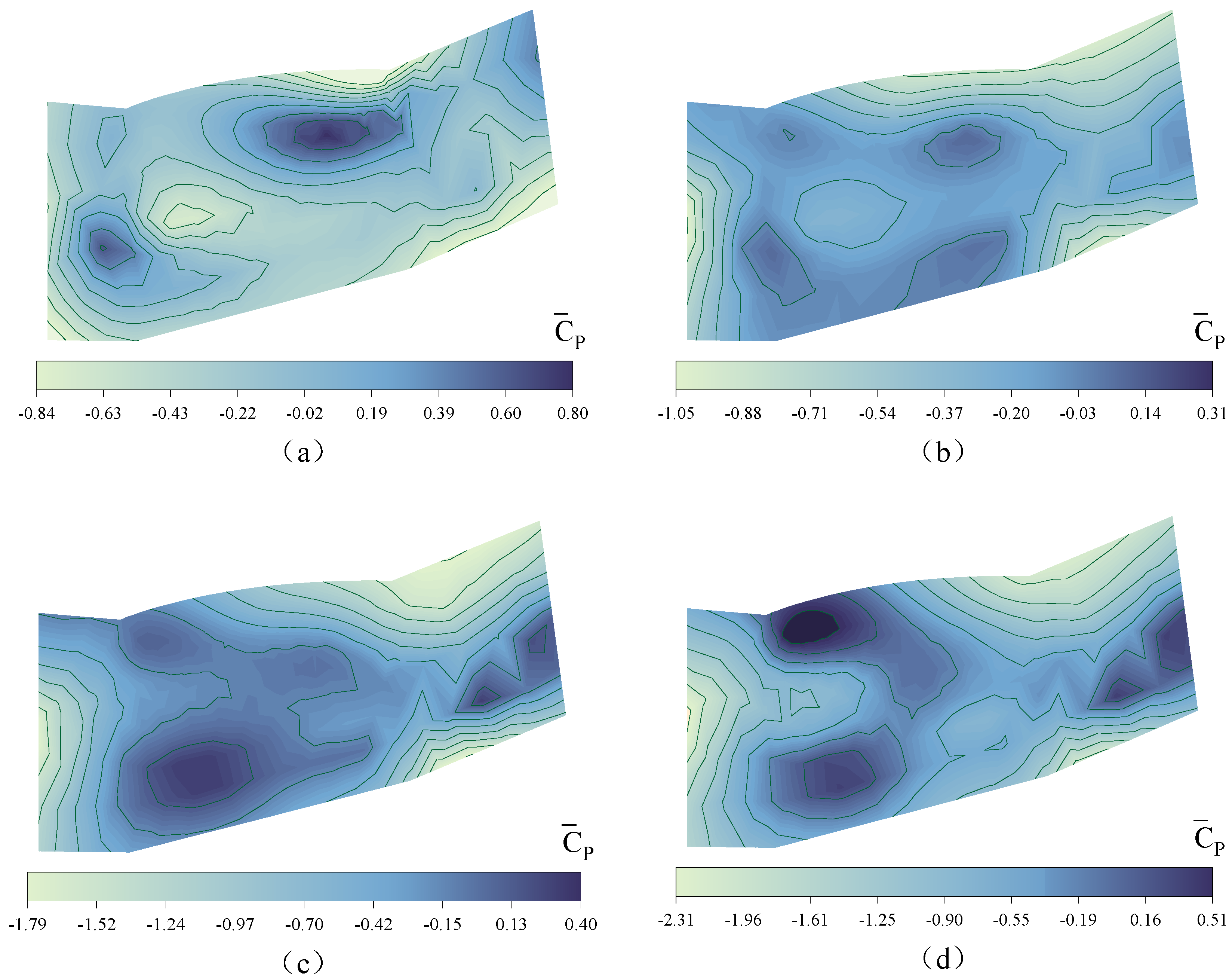
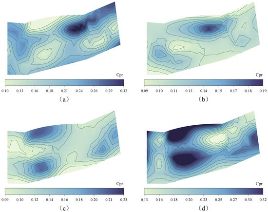
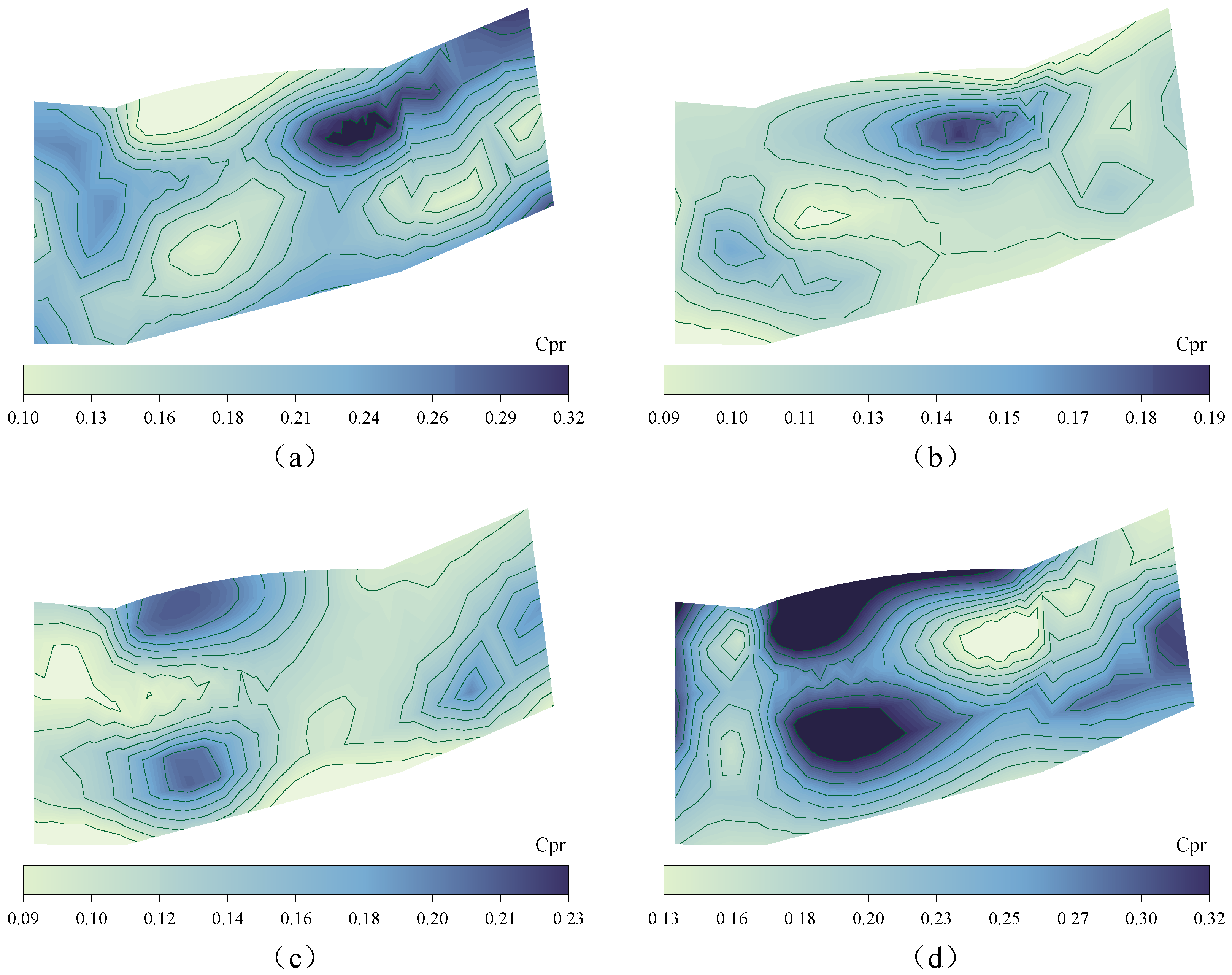
According to Equations (2) and (3), the ${\overline{C}}_p$ and $C_{p\mathrm{r}}$ values of the points arranged on the glass curtain wall model of the coastal airport terminal can be derived for different wind angles, and next, the ${\overline{C}}_p$ and $C_{p\mathrm{r}}$ values of the right half of the glass curtain wall are discussed using typical wind angles of $0^{\circ }$, ${45}^{\circ }$, ${135}^{\circ }$ and ${180}^{\circ }$ as examples. As shown in Figure 7 and Figure 8, it is easy to see that most of the measurement points on the windward side of the glass curtain wall show positive pressure values, while relatively speaking, at the edges, corners or other large areas of the curtain wall, the measurement points show negative pressure values. Moreover, the ${\overline{C}}_p$ and $C_{p\mathrm{r}}$ values at the transition of the corners of the glass curtain wall have very obvious changes; especially when the curtain wall is at wind angles of $0^{\circ }$ and ${180}^{\circ }$, the measured ${\overline{C}}_p$ and $C_{p\mathrm{r}}$ values are higher compared to the curtain wall at wind angles of ${45}^{\circ }$ and ${135}^{\circ }$, with the ${\overline{C}}_p$ reaching up to 0.80 and the $C_{p\mathrm{r}}$ reaching up to 0.32.

Figure 7. Cloud map of mean wind pressure coefficient distribution on the surface of the glass curtain wall under wind direction angles (a) 0°; (b) 45°; (c) 90°; (d) 180°.

Figure 8. Cloud map of fluctuating wind pressure coefficient distribution on the surface of the glass curtain wall under wind direction angles of (a) 0°; (b) 45°; (c) 90°; (d) 180°.

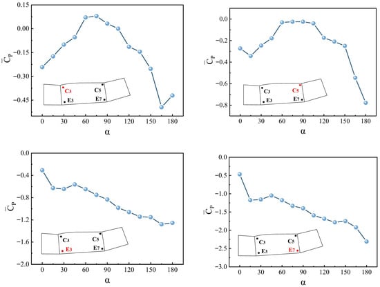
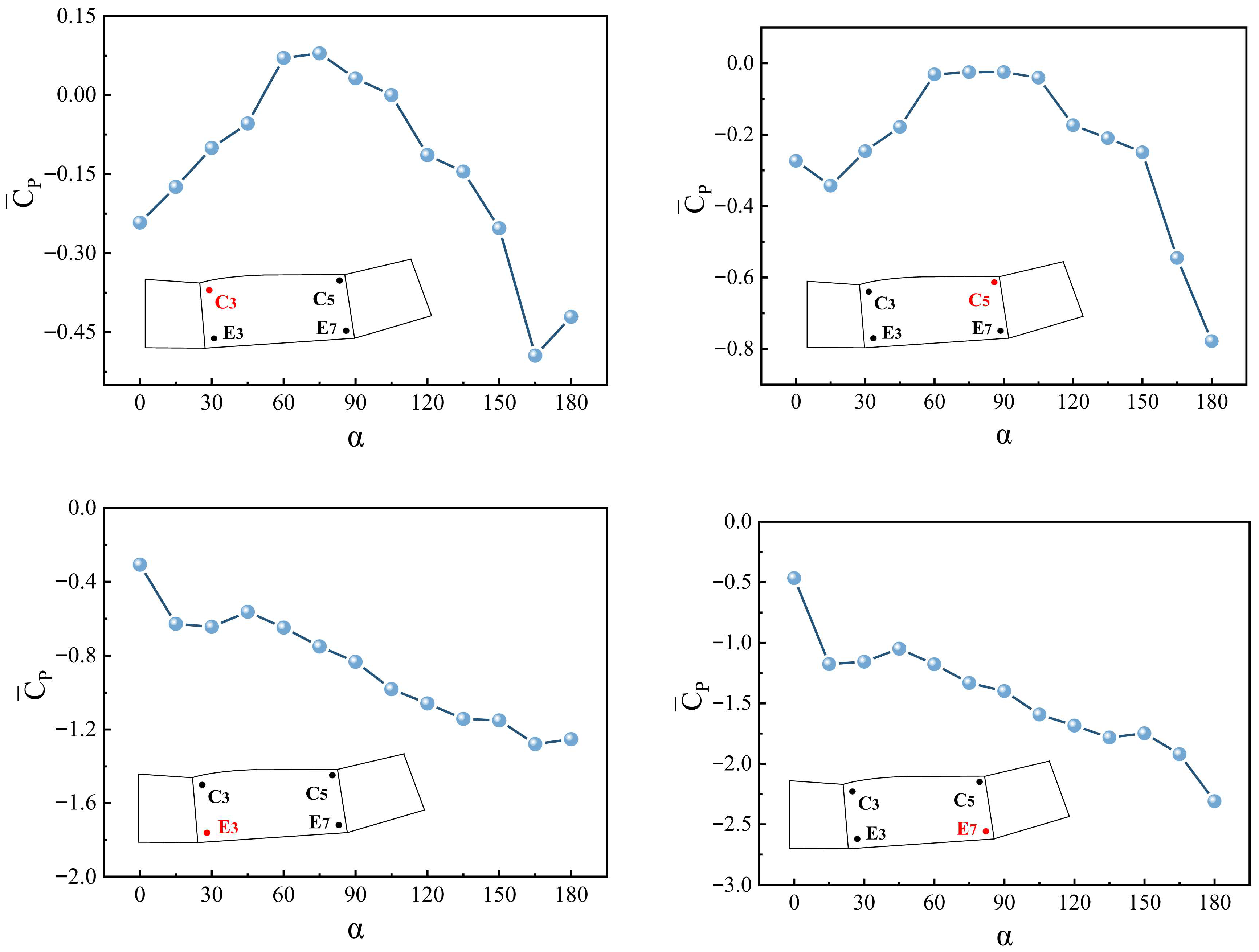
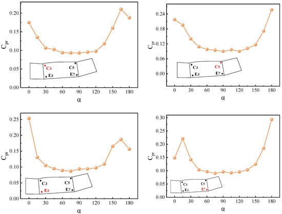
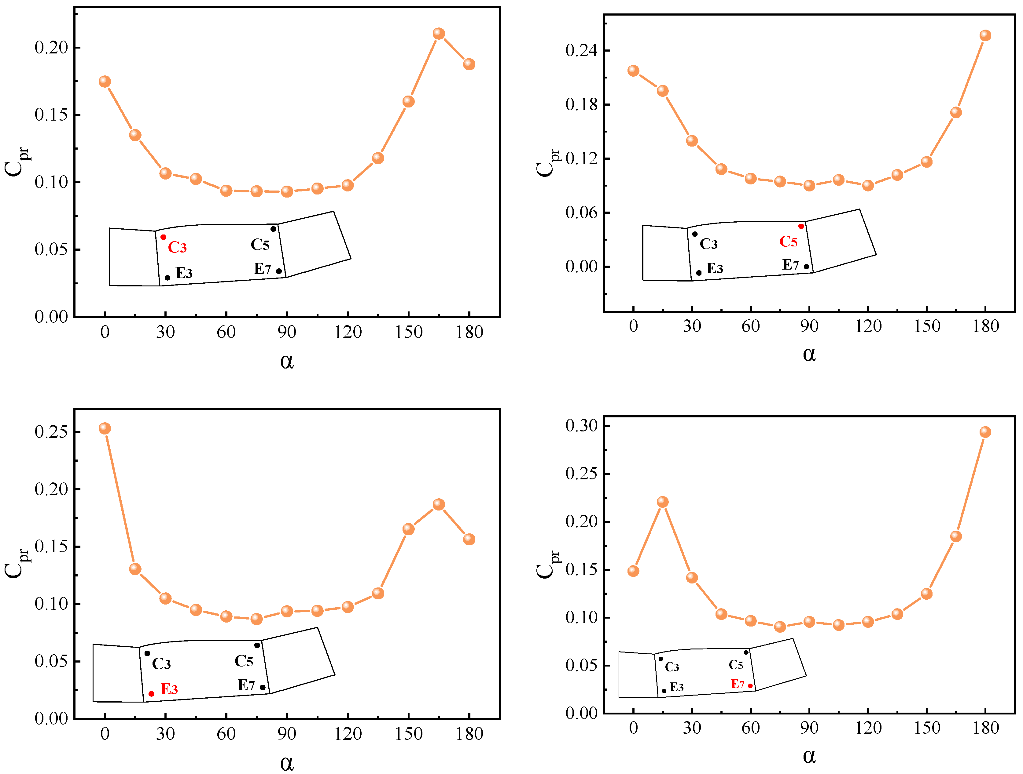
In order to observe more intuitively the changes of ${\overline{C}}_p$ and $C_{p\mathrm{r}}$ values under different wind angles, based on the results presented in the cloud map, four points located at the corner edges of the curtain wall, C₃, C₅, E₃ and E₇, were selected as typical measurement points for the study, and Figure 9 and Figure 10 are plotted with 12 different wind angles set at every ${15}^{\circ }$ as the horizontal coordinates. From the figure, it can be observed that the ${\overline{C}}_p$ values of points C₃ and C₅ located on the upper edge of the curtain wall corner and points E₃ and E₇ located on the lower edge are mostly negative. Under the change in the wind direction angle, they show similar trends and show a clear downward trend in a certain wind direction angle range. The common point can also be observed in the $C_{p\mathrm{r}}$ values of the four points, none of which produced large fluctuations in the wind angle interval from ${45}^{\circ }$ to ${135}^{\circ }$, showing a curve with a gentle transition, but near the two wind angle intervals of $0^{\circ }$ and ${180}^{\circ }$, the $C_{p\mathrm{r}}$ values corresponding to the four points are all relatively higher.

Figure 9. Variation diagram of mean wind pressure coefficient of typical measuring points C₃, C₅, E₃ and E₇ on the surface of glass curtain wall varies with wind direction angle.

Figure 10. Variation diagram of fluctuating wind pressure coefficient of typical measuring points C₃, C₅, E₃ and E₇ on surface of glass curtain wall with wind direction angle.

4.2. Wind Pressure Coefficient Prediction

In the preceding section, the mean and fluctuating wind pressure coefficients of typical measurement points situated at the upper and lower edges of the glass curtain wall at the side corners of the airport terminal building were examined. In the following section, the wind pressure coefficients of the two points on the glass curtain wall at the wind direction angles of C₃ and C₅ were selected for prediction. Among the available prediction methods, the use of a neural network model is currently the most popular approach. CNN in particular is a highly matured neural network model that has demonstrated significant advantages in prediction tasks. Additionally, the Transformer model, which is currently emerging in the field, has also exhibited a remarkable capacity to handle time series data.

This paper presents three scenarios of CNN, Transformer and CNN–Transformer combination models selected for wind pressure coefficient prediction. The relevant model parameter settings are shown in Table 1. These parameters were determined through hyperparameter search. The measured wind pressure coefficient time series was employed in the study, with 20% of the dataset utilized for testing and the remaining 80% designated as the training set. Data were collected for 200 s at each measurement point, resulting in a total of 102,400 data points (200 × 512) for each location.

Table 1. Parameter settings for CNN, Transformer, and CNN–Transformer models.

Parameter	CNN	Transformer	CNN–Transformer
Training batch scale	32	32	32
Optimizer	Adam	Adam	Adam
Number of training iterations	30	30	30
Activation function	Relu	Relu	Relu
Learning rate	10−4	10−4	10−4

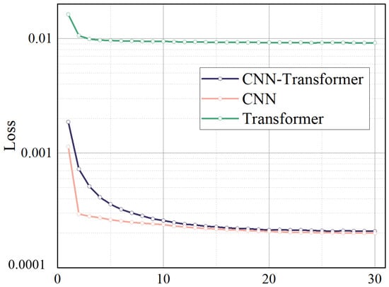
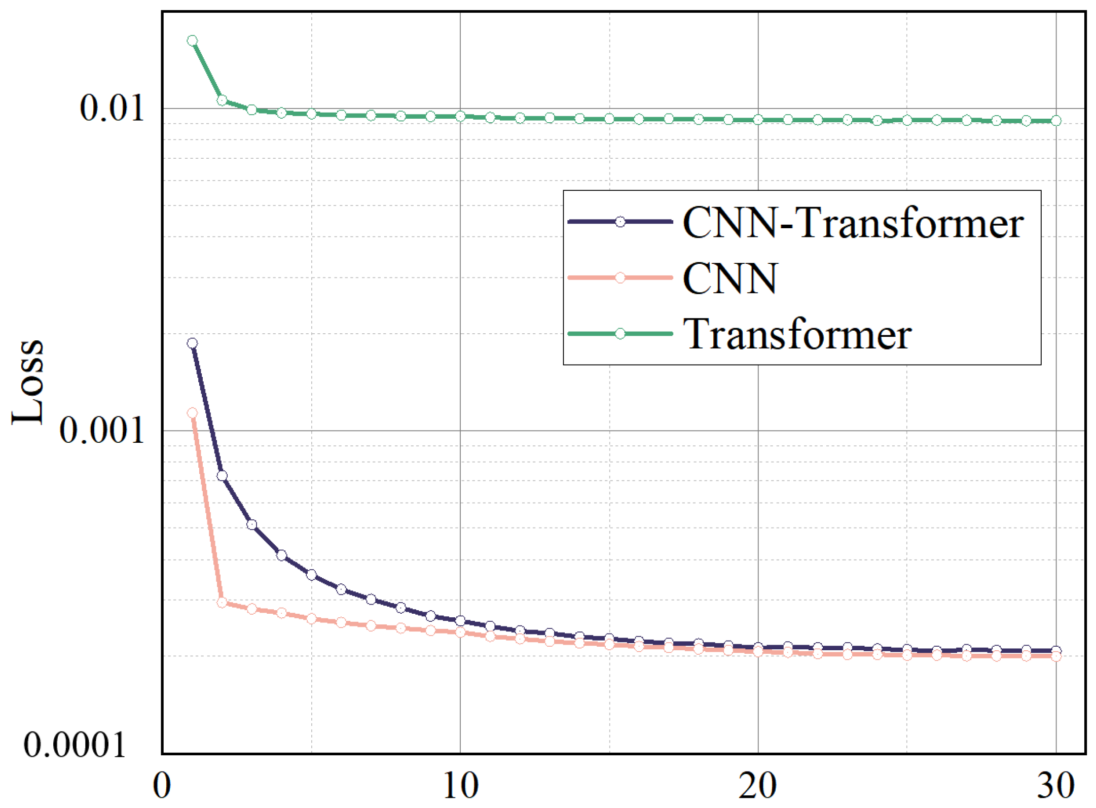
The selection of the learning rate in neural network training presents a critical trade-off between the convergence rate and solution stability. While higher values accelerate model convergence, they risk inducing oscillatory behavior near optimal solutions. Conversely, lower values promote stable convergence at the expense of computational efficiency. This study systematically evaluated three distinct architectures—CNN, Transformer, and their hybrid CNN–Transformer model—through multiple training trials. Figure 11 presents representative loss function trajectories, demonstrating that all architectures achieve stable convergence after sufficient iterations, with the hybrid model exhibiting particularly robust performance.

Figure 11. Loss function diagrams corresponding to different prediction models under the same number of iterations.

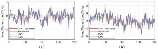
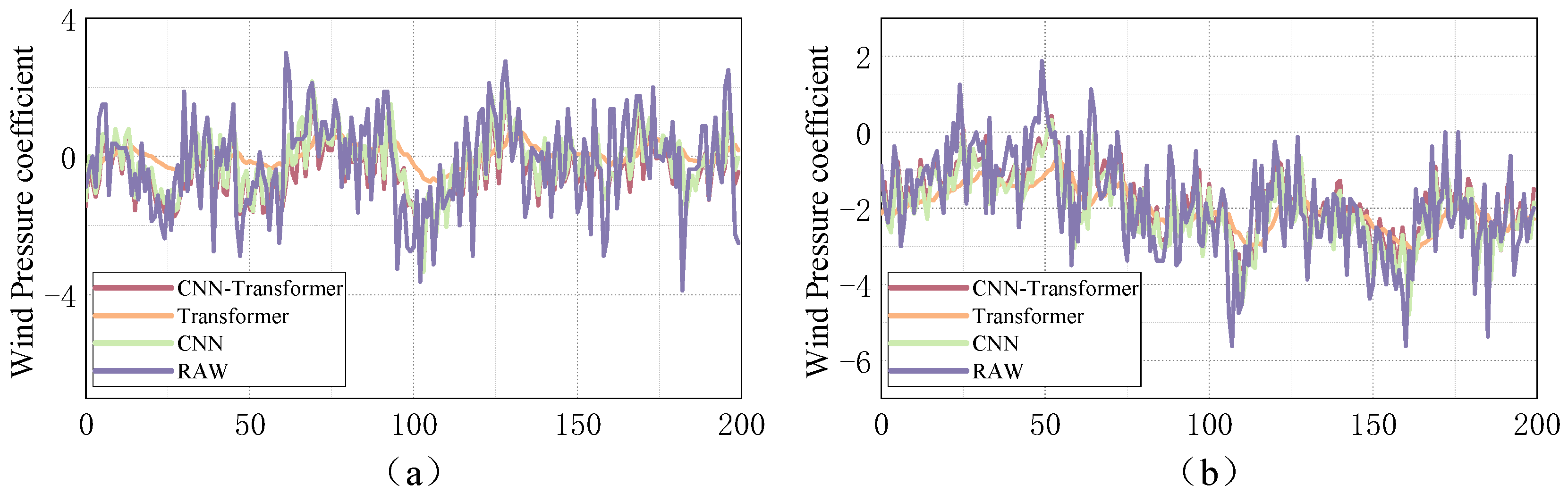
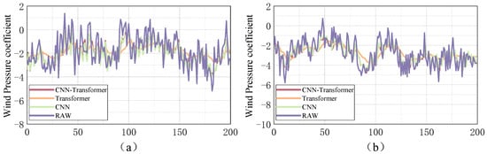
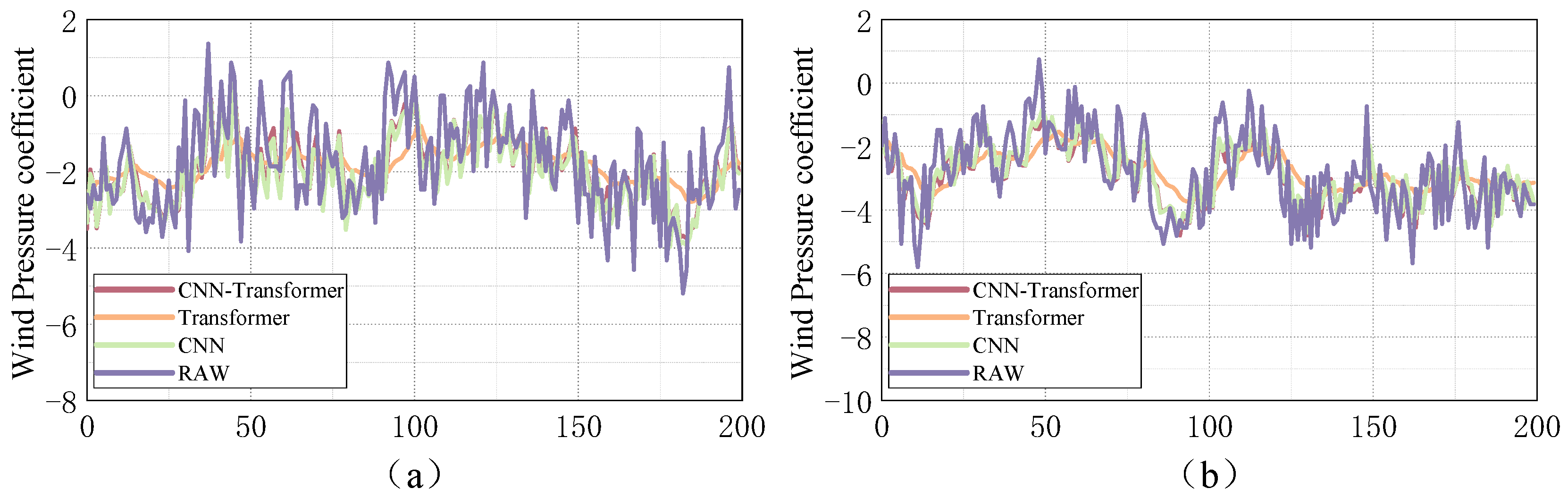
Figure 12 and Figure 13 compare the true and predicted wind pressure values. All three models yield results close to the true values, with Transformer performing the worst, the CNN the second best, and the CNN–Transformer hybrid model the most accurate. The standalone Transformer only captures the general trend but performs poorly at extreme values, leading to large deviations. The CNN better extracts key features and outperforms the Transformer. Combining their advantages, the proposed CNN–Transformer model achieves superior prediction, more accurate peaks, and better consistency with true trends. Under different wind angles and measurement points, the hybrid model still shows smaller deviations than the other two models. It also requires less training time while achieving higher accuracy. Thus, the CNN–Transformer model enables more efficient and reliable wind pressure coefficient prediction.

Figure 12. Wind pressure coefficient prediction diagram of point C₃ on the surface of the glass curtain wall using different prediction models at wind angles of (a) 45°; (b) 135°.

Figure 13. Wind pressure coefficient prediction diagram of point C₅ on the surface of the glass curtain wall using different prediction models at wind angles of (a) 45°; (b) 135°.

4.3. Assessment of Methods for Predicting Wind Pressure

To conduct a comprehensive quantitative evaluation of the predictive performance across the three model architectures, this study employs two statistically robust error metrics for systematic analysis. These selected evaluation criteria—specifically, the mean absolute error (MAE) and root mean square error (RMSE)—provide distinct yet complementary measures of prediction accuracy. The mathematical formulations of these metrics are presented below, enabling precise comparison of model performance.

$$MAE={\displaystyle \frac{1}{N}}{\displaystyle {\sum }_{t=1}^T\left|Y_t-{\widehat{Y}}_t\right|}$$

(4)

$$RMSE=\sqrt{{\displaystyle \frac{1}{N}}{\displaystyle {\sum }_{t=1}^T(Y_t-{\widehat{Y}}_t}{)}^2}$$

(5)

In the formula, $Y_t$ is the measured value at time step t, ${\widehat{Y}}_t$ indicates the model’s predicted output for the same temporal interval, ${\overline{Y}}_t$ signifies the mean value computed from all empirical observations, and $N$ is the total number of predicted instances included in the validation dataset.

The outcomes of each round of wind pressure coefficient forecasting at points C₃ and C₅ at 45° and 135° wind angles were collated, and the values of MAE and RMSE were calculated and are summarized in Table 2.

Table 2. Summary of error metrics for CNN, Transformer, and CNN-Transformer prediction models.

Point	Wind Direction Angle	Index	Model	Value
C3	45$°$	MAE	CNN	0.90
			Transformer	0.96
			CNN–Transformer	0.80
		RMSE	CNN	1.10
			Transformer	1.30
			CNN–Transformer	1.00
	135$°$	MAE	CNN	0.64
			Transformer	0.87
			CNN–Transformer	0.58
		RMSE	CNN	0.77
			Transformer	1.09
			CNN–Transformer	0.73
C5	45$°$	MAE	CNN	0.71
			Transformer	0.87
			CNN–Transformer	0.68
		RMSE	CNN	0.88
			Transformer	1.03
			CNN–Transformer	0.84
	135$°$	MAE	CNN	0.53
			Transformer	0.83
			CNN–Transformer	0.49
		RMSE	CNN	0.69
			Transformer	1.24
			CNN–Transformer	0.67

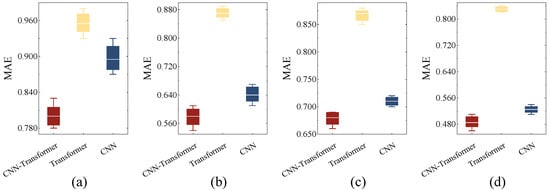
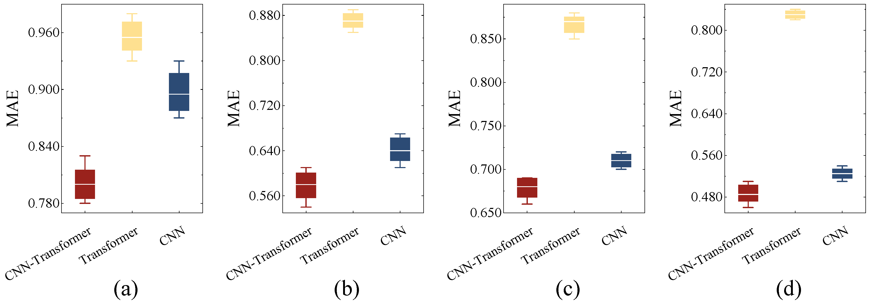
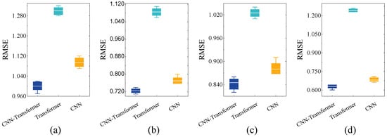
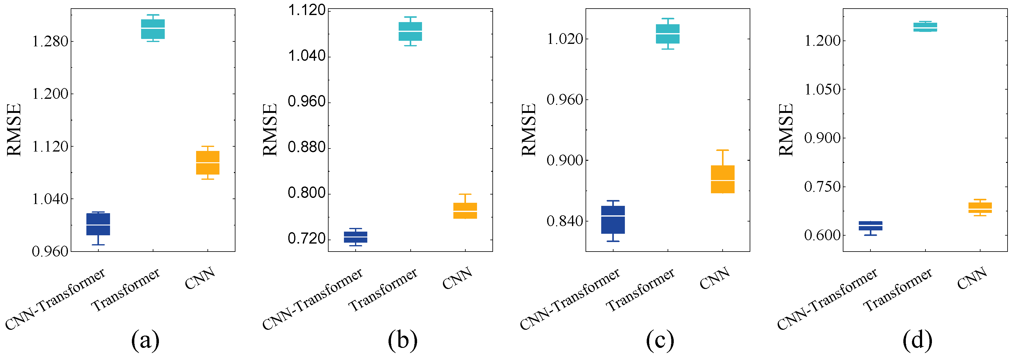
From Table 2 and the error analysis in Figure 14 and Figure 15, it can be seen that under different prediction scenarios, the MAE of the CNN model fluctuates between 0.53 and 0.90, and the RMSE fluctuates between 0.69 and 1.10; The MAE of the Transformer model fluctuates between 0.83 and 0.96, while the RMSE fluctuates between 1.03 and 1.30. The MAE of the CNN–Transformer model fluctuates between 0.49 and 0.80, while the RMSE fluctuates between 0.67 and 1.00. Among the three models, the CNN–Transformer model has the lowest MAE value of 0.49, and the CNN–Transformer model also has the lowest RMSE value of 0.67.

Figure 14. MAE schematic diagram of measuring points C₃ and C₅ on the surface of the glass curtain wall using different prediction models at wind angles of ${45}^{\circ }$ and ${135}^{\circ }$. Note: (a,b) wind angles of ${45}^{\circ }$ and ${135}^{\circ }$ (C₃); (c,d) wind angles of ${45}^{\circ }$ and ${135}^{\circ }$ (C₅).

Figure 15. RMSE schematic diagram of measuring points C₃ and C₅ on the surface of the glass curtain wall using different prediction models at wind angles of ${45}^{\circ }$ and ${135}^{\circ }$. Note: (a,b) wind angles of ${45}^{\circ }$ and ${135}^{\circ }$ (C₃); (c,d) wind angles of ${45}^{\circ }$ and ${135}^{\circ }$ (C₅).

In comparison with the Transformer model exhibiting the highest MAE and RMSE values, the CNN–Transformer combination model has demonstrated an enhanced degree of prediction accuracy, with improvements of 41% and 33%, respectively. In this study on the prediction of wind pressure coefficients, the combined prediction model of CNN–Transformer consistently outperforms the single models of CNN and Transformer. Its superiority is evident regardless of the location of measuring points or the size of the wind direction angle. It may be posited that the CNN–Transformer model is universally applicable in the prediction of wind pressure coefficients and is capable of accurately predicting the wind pressure coefficients of any measuring point on the glass curtain wall at varying wind direction angles. Moreover, the prediction of the wind pressure coefficient on the surface of the glass curtain wall allows for the subsequent calculation of the wind pressure magnitude, thereby providing data support for the safe operation of the terminal building and ensuring the safety of passengers in extreme weather conditions such as strong winds.

4.4. CFD Simulation Results

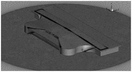
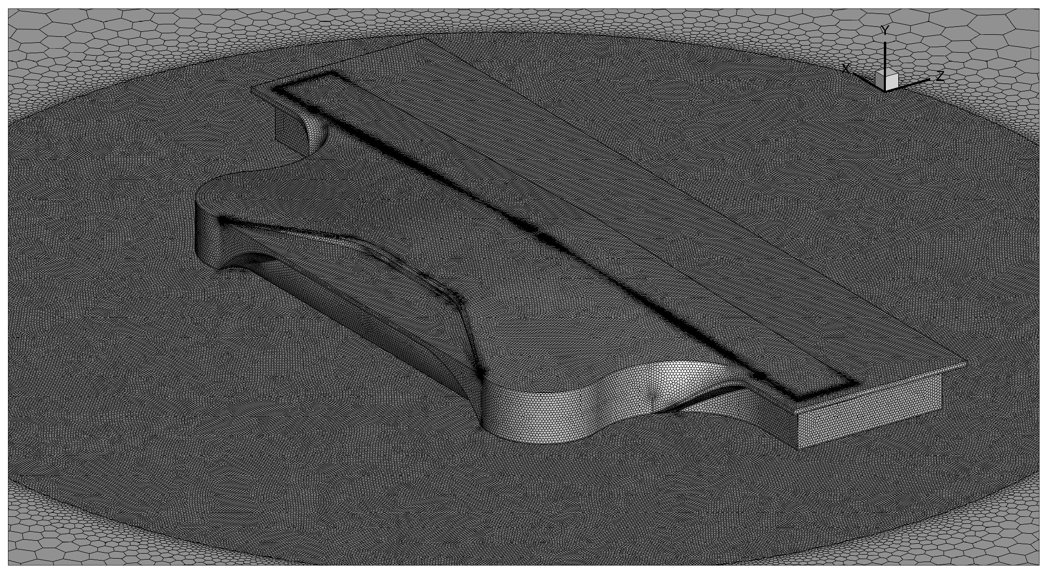
In this study, the aerodynamic flow around the airport building was simulated under incoming crosswind conditions. A sufficiently large computational domain was established to reduce the influence of artificial boundary effects on the flow around the structure. The inlet boundary of the flow field was prescribed as a velocity-inlet boundary, while the outlet was defined as a pressure-outlet boundary. The lateral and top boundaries of the computational domain were treated as symmetry boundaries. The airport building and ground surface were modeled as no-slip walls. Considering computational efficiency and the characteristics of turbulence models for separated external flows, the shear-stress transport (SST) k–ω model was selected for the present simulations. This model provides improved accuracy in predicting near-wall flow behavior and local separation around bluff and streamlined structural components. The mesh was generated using an unstructured hybrid meshing approach, with local refinement applied near the airport building and in wake regions where strong velocity gradients were expected. In addition, boundary-layer meshes were generated on the building surface with 15 layers, and the growth rate was set to 1.2 to ensure a smooth transition from the near-wall region to the outer flow field. The near-wall mesh resolution was controlled such that the y+ values remained below 1 over the building surfaces, thereby satisfying the requirements for accurate wall-resolved simulations with the SST k–ω model. The mesh details of the airport model are shown in Figure 16.

Figure 16. Grid layout.

A transient solver was employed to capture the unsteady aerodynamic characteristics of the flow around the building. The time step was set to 0.0001 s, and the residual convergence criterion for each time step was specified as 10⁻⁴. The pressure coefficients obtained from the numerical simulations are in good agreement with those measured in the wind tunnel tests, which demonstrates the validity of the adopted CFD model.

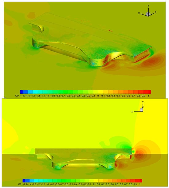
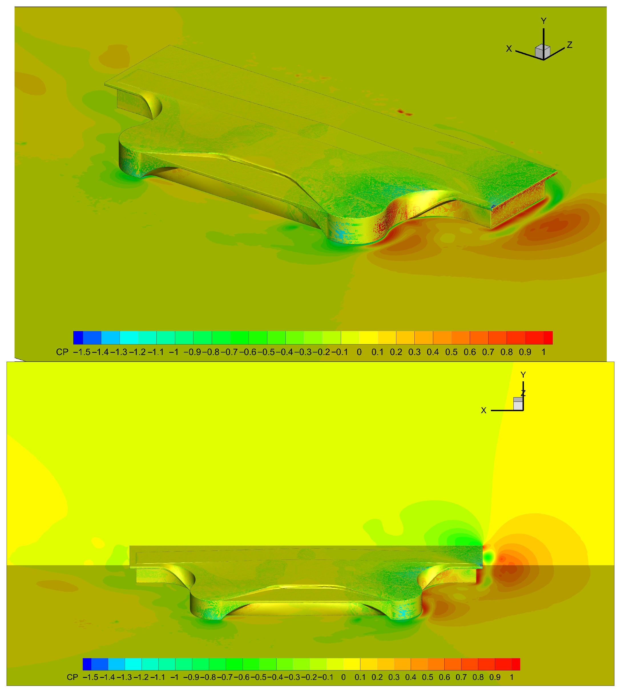
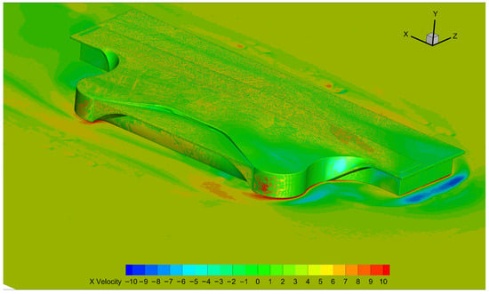
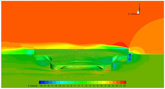
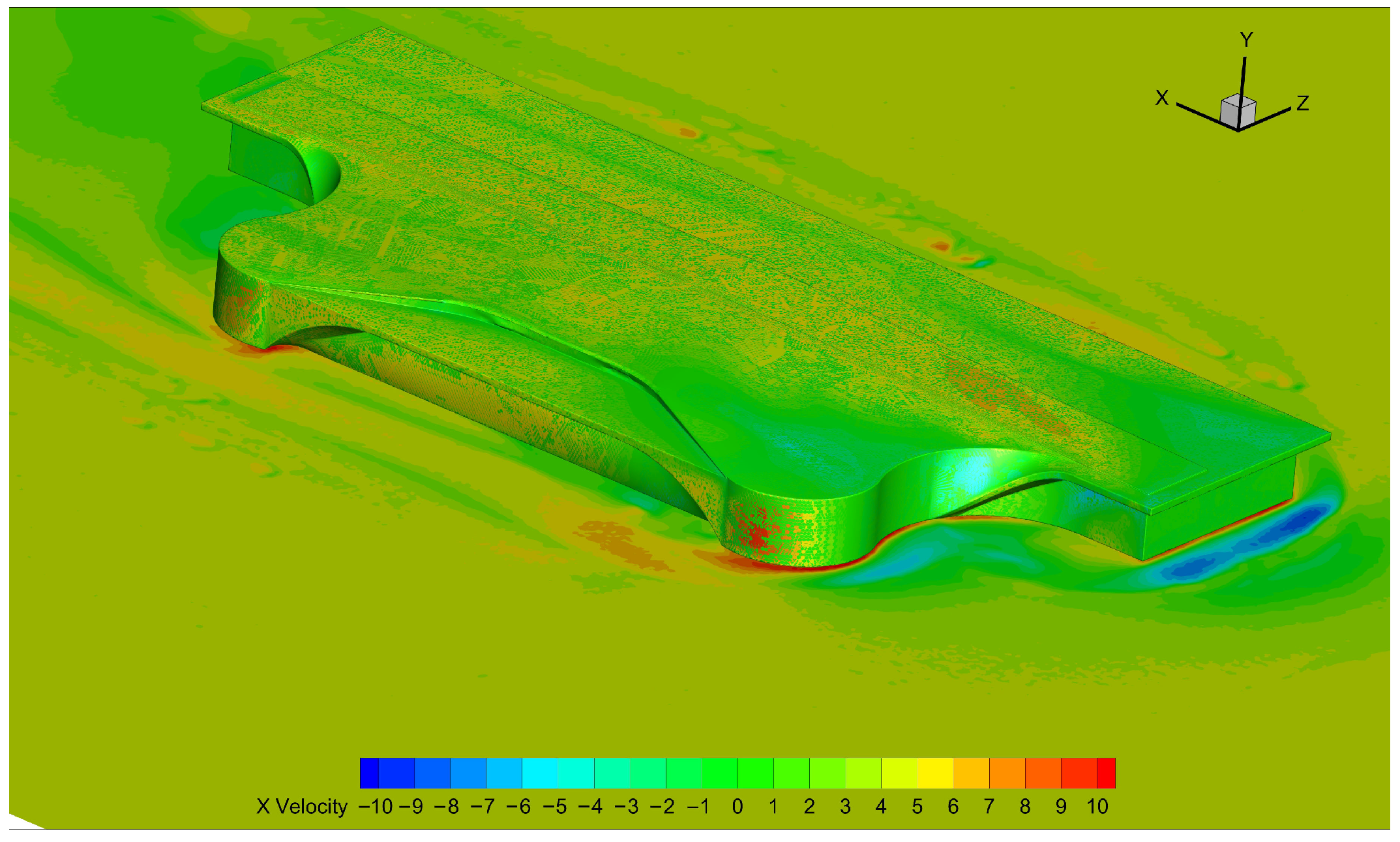
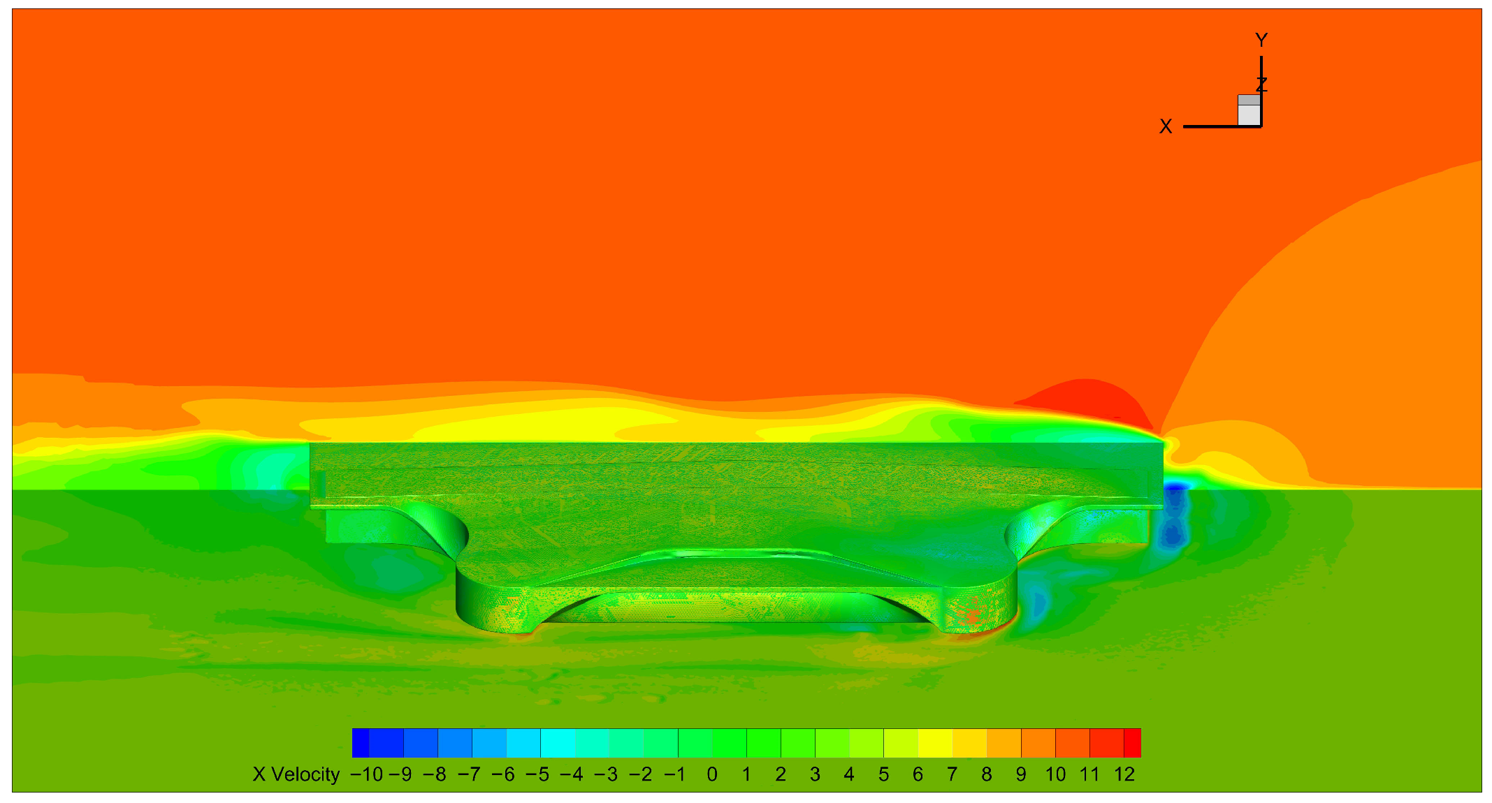
In order to provide a more intuitive description of the wind pressure distribution characteristics of the airport terminal model, high-precision modeling and simulation were carried out using CFD. The grid division is shown in Figure 16. From the CFD simulation results in Figure 17 and Figure 18, it can be seen that under various operating conditions, there is a large negative pressure on the leading edge of the roof at the windward position, while the negative pressure on the other side of the roof is very small, even positive pressure.

Figure 17. Airport surface pressure coefficient (0 deg).

Figure 18. Velocity flow field (0 deg).

5. Conclusions

Based on the wind tunnel test data collected from the surface of the glass curtain wall of an airport terminal building, this paper conducts research on wind pressure prediction. Firstly, the characteristics of average wind pressure and fluctuating wind pressure at typical measurement points of the glass curtain wall are analyzed; secondly, a combined CNN–Transformer prediction model is constructed, and the model is trained and tested for performance; and finally, the prediction results of the combined model are compared with those of the single CNN and Transformer models, and the error indicators of the three models are analyzed, leading to the following research conclusions:

1. The calculation results show that the wind pressure values at the edge and corner measurement points of the glass curtain wall of the airport terminal building (wind-pressure-related parameters not clearly specified in the original text) vary most significantly with changes in wind angle; among them, most measurement points on the windward side of the curtain wall show positive values, while the remaining measurement points show negative values.

2. Through the comparative analysis of the two error indicators, MAE and RMSE, the combined CNN–Transformer prediction model performs better than the single CNN model and the single Transformer model in wind pressure prediction; in addition, the combined model exhibits higher prediction accuracy in wind pressure prediction at different measurement points under different wind angles, indicating that the proposed CNN–Transformer integrated prediction model has universal applicability.

3. This paper adopts a combination of wind tunnel tests and neural network models to conduct research on the wind pressure of the glass curtain wall of airport terminal buildings, which can provide valuable references for the engineering design and construction of the enclosure structure of airport terminal buildings in the future.

At present, most of the research on the wind pressure distribution characteristics and prediction of airport terminal buildings focuses on long-span roofs, while the relevant research on glass curtain walls is relatively scarce. This is a weak point in the current research field, and it also points out the direction for the follow-up research of this paper and further exploration in related fields.

References

- Gerhardt, H.J.; Kramer, C. Wind loads on wind-permeable building facades. J. Wind Eng. Ind. Aerodyn. 1983, 11, 1–20. [Google Scholar] [CrossRef] [Scilit]
- Gomes, M.G.; Silva, F.M. Multi-storey double-skin facades influence on surface pressure distribution. In Proceedings of the CISBAT 2004, Lausanne, Switzerland, 7–9 July 2004; pp. 107–122. [Google Scholar]
- Kawai, H. Wind loads on double skin facades with opening windows. In Proceedings of the Sixth Asia-Pacific Conference on Wind Engineering, Seoul, Republic of Korea, 12–14 September 2005; pp. 231–247. [Google Scholar]
- Kim, Y.C.; Yoshida, A.; Tamura, Y. Characteristics of surface wind pressures on low-rise building located among large group of surrounding buildings. Eng. Struct. 2012, 35, 18–28. [Google Scholar] [CrossRef] [Scilit]
- Chen, F.B.; Li, Q.S. Characteristics of wind loads acting on complex long-span roof structure. Adv. Mater. Res. 2013, 639, 523–529. [Google Scholar] [CrossRef] [Scilit]
- Liu, Y.; Kopp, G.A.; Chen, S.F. Effects of Plan Dimensions on Gust Wind Loads for High-Rise Buildings. J. Wind Eng. Ind. Aerodyn. 2019, 194, 103980. [Google Scholar] [CrossRef] [Scilit]
- Sun, X.; Yu, R.; Wu, Y. Investigation on wind tunnel experiments of ridge-valley tensile membrane structures. Eng. Struct. 2019, 187, 280–298. [Google Scholar] [CrossRef] [Scilit]
- Wu, Y.; Wu, X.; Wei, S.; Sun, Q.; Wang, J. Experimental study of wind pressure fluctuating characteristics and wind load shape factor of long-span cylinder roof structure. Struct. Des. Tall Spec. Build. 2021, 30, e1860. [Google Scholar] [CrossRef] [Scilit]
- Yang, X.; Zhou, Q.; Lei, Y.; Yang, Y.; Li, M. Non-Gaussian features of dynamic wind loads on a long-span roof in boundary layer turbulences with different integral-scales. Wind Struct. 2022, 34, 421–435. [Google Scholar] [CrossRef] [Scilit]
- Tian, J.; Gurley, R.K.; Diaz, T.M.; Fernández-Cabán, P.L.; Masters, F.J.; Fang, R. Low-rise gable roof buildings pressure prediction using deep neural networks. J. Wind Eng. Ind. Aerodyn. 2020, 196, 104026. [Google Scholar] [CrossRef] [Scilit]
- Chen, F.; Kang, W.; Shu, Z.; Li, Q.; Li, Y.; Chen, Y.F.; Zhou, K. Predicting roof-surface wind pressure induced by conical vortex using a BP neural network combined with POD. Build. Simul. 2021, 15, 1475–1490. [Google Scholar] [CrossRef] [Scilit]
- Vigneshwaran, R.; Prabavathy, S.; Sivasubramanian, J. Prediction of Wind-Induced Pressure on Pentagon Plan Shape Building using Artificial Neural Network. J. Inst. Eng. (India) Ser. A 2022, 103, 581–599. [Google Scholar] [CrossRef] [Scilit]
- Ding, Z.; Zhang, W.; Zhu, D.L. Neural-network based wind pressure prediction for low-rise buildings with genetic algorithm and Bayesian optimization. Eng. Struct. 2022, 260, 114203. [Google Scholar] [CrossRef] [Scilit]
- Chen, F.B.; Wang, X.L.; Li, X.; Shu, Z.R.; Zhou, K. Prediction of wind pressures on tall buildings using wavelet neural network. J. Build. Eng. 2022, 46, 103674. [Google Scholar] [CrossRef] [Scilit]
- Huang, Y.; Wu, H.; Fu, J.; Zhang, H.; Li, H. Convolutional neural network-based wind pressure prediction on low-rise buildings. Eng. Struct. 2024, 309, 118078. [Google Scholar] [CrossRef] [Scilit]
- Huang, X.J.; Li, S.Q.; Han, L.X. Prediction of wind pressures on supertall buildings based on proper orthogonal decomposition and machine learning. Struct. Des. Tall Spec. Build. 2024, 33, e2174. [Google Scholar] [CrossRef] [Scilit]
- GB50009-2012; Load Code for the Design of Building Structures. China Architecture & Building Press: Beijing, China, 2012.
Disclaimer/Publisher’s Note: The statements, opinions and data contained in all publications are solely those of the individual author(s) and contributor(s) and not of MDPI and/or the editor(s). MDPI and/or the editor(s) disclaim responsibility for any injury to people or property resulting from any ideas, methods, instructions or products referred to in the content. |
© 2026 by the authors. Licensee MDPI, Basel, Switzerland. This article is an open access article distributed under the terms and conditions of the Creative Commons Attribution (CC BY) license.