A Case Study on Response Characteristics of Large Steel Frame Support Structures Under the Combined Action of Earthquake and Wind Loads, Considering Shielding Effects

Abstract

Large steel frame support structures may encounter multiple-hazard coupling effects, such as earthquakes and wind loads, during their service period, and their combined damage effects are often significantly greater than those under single-hazard conditions. This study focuses on a single case example of large steel frame support structures, adopts a one-way CFD (Computational Fluid Dynamics)-to-structure loading analysis method to quantify the distribution of wind drag coefficients influenced under shielding effects, and reveals the response amplification and transition behavior under earthquake–wind load coupling effects through a systematic parametric analysis. The results demonstrate that within the simulated wind speed range (10–30 m/s), the drag coefficient of the structure is insensitive to the Reynolds number. The drag coefficient of the first row of members remains stable at approximately 1.25, whereas those of the second and subsequent rows are concentrated in the 0.6–0.8 range and decrease progressively along the wind direction. This pattern challenges the conventional design assumption of using a unified drag coefficient. Based on the analyzed cases, under earthquake–wind coupling effects, the structural amplitude amplification effect demonstrates significant load-dominant transition characteristics—when the earthquake acceleration is low (0.05 g), the wind load-induced amplitude amplification effect is pronounced, reaching 206.3%. As the earthquake intensity increases, the amplification effect stabilizes at approximately 9%. This study identifies structural drag coefficients for considering shielding effects, reveals the coupling mechanism between earthquakes and wind loads, and provides theoretical support for the multihazard performance-based design of temporary large-scale spatial structures. It should be noted that the findings and the proposed load-dominance transition characteristics are primarily applicable to temporary large-scale spatial frame structures operating within a service wind speed range of 10 to 30 m/s.

1. Introduction

In recent years, global warming and intensified geological activity have led to the frequent occurrence of extreme multihazard events [1]. In addition to single disasters, the probability of coupled effects between earthquakes and strong winds has significantly increased, becoming a new challenge that cannot be ignored in the field of engineering disaster prevention [2,3,4]. In accordance with the Beaufort wind scale, wind speeds exceeding 10 m/s are defined as strong winds [5]. On 12 October 2019, during the landfall of Super Typhoon Hagibis in Chiba Prefecture, Japan, extreme wind fields with maximum speeds reaching 42 m/s occurred almost simultaneously with a magnitude 5.7 earthquake, resulting in significant casualties and structural damage. This typical case highlights the real threat of multihazard coupling effects. Research has indicated that significant changes in atmospheric pressure fields often occur before and after earthquakes and are potentially accompanied by severe weather events [6]. Lin et al. [7] reported a 63.75% correlation based on a statistical analysis of 102 typhoon–earthquake events near Taiwan, China, over 15 years. Through statistical studies in Yunnan, China, Li et al. [8] confirmed that the concurrent probability of earthquakes and strong winds cannot be ignored. Through a systematic review of 120 years of earthquake data from 1901–2020, Yu et al. [9] identified 218 concurrent events with magnitudes exceeding 4 and wind speeds surpassing 10 m/s. Furthermore, earthquakes can induce localized strong winds through mechanisms such as atmospheric temperature anomalies and electromagnetic wave disturbances, further corroborating the potential nonlinear relationships between these two types of disasters [10].

However, current design codes significantly lag behind the reality of disasters in terms of the coupled effects of earthquakes and wind. The European code EN 1990 [11] and American code ASCE 7-22 [12] do not account for the combined effects, assuming a low probability of their simultaneous occurrence; meanwhile, the current Chinese code [13] only applies a simplified combination coefficient of 0.2 for wind-sensitive high-rise buildings. This gap in code-level understanding may lead to an overestimation of the actual safety reserves of structures under multihazard conditions. Therefore, revealing the structural dynamic response mechanisms under earthquake–wind coupling effects, scientifically assessing the threats of extreme compound disasters, and providing theoretical foundations for disaster-resistant design and performance optimization are urgently needed and have significant scientific value [14].

Currently, studies on structural multihazard responses have achieved abundant results, but there is a significant bias in research subjects. In terms of single hazards, scholars have extensively studied structural performance under earthquakes, hurricanes, floods, etc. [15,16,17,18,19,20,21]. In terms of multihazard coupling, researchers have conducted studies on the theoretical frameworks for seismic–wind interaction analysis [10,22,23], as well as on conventional structural systems such as low- to medium-rise buildings, high-rise buildings, bridges, and wind turbines [24,25,26,27,28,29]. Sibille et al. [30] investigated the effects of environmental loads such as ship impact and wind load on the steel frame structure of a ferry terminal through structural health monitoring (SHM). Additionally, numerous researchers analyzed and predicted the seismic damage of structures based on machine learning algorithms [31,32]. Nevertheless, insufficient attention has been given to large temporary steel frame support structures, which constitute a unique and important category of engineering structures.

Large steel frame support structures, as critical temporary facilities for major social events and engineering projects, are widely used in scenarios such as the Spring Festival Gala stages, Winter Olympics opening ceremonies, large-scale concerts, electronic display screen supports, and outdoor construction protection. These structures typically employ a spatial steel truss system composed of columns and horizontal steel pipes, characterized by their tall and open design, lightweight yet strong construction, and large height–width ratios, leading to high sensitivity to both wind loads and seismic actions. Owing to their short service cycles, high reuse rates, and variable site conditions, design priorities often emphasize functionality and construction efficiency, with insufficient attention given to performance-based design against multiple hazards. The limitations of existing research directly result in a lack of understanding of the failure mechanisms of such structures under coupled seismic–wind environments, hindering the development of optimized disaster-resistant designs and risk management strategies and thereby posing potential safety threats to users. Therefore, focusing on large steel frame support structures as unique subjects, this study reveals the response amplification and transition behavior under earthquake–wind load coupling effects through a systematic parametric analysis, which is a crucial step to fill theoretical gaps, improve standard systems, and ensure public safety.

The majority of existing studies either adopt simplified wind load models or neglect the shielding-effect-modulated drag coefficient distribution in dense spatial frame systems, leading to inaccurate wind load predictions for such structures. Considering the shielding effects, this study integrates full-scale refined Finite Element Model (FEM) to systematically study the dynamic response characteristics of large temporary spatial steel frame support systems under combined earthquake–wind actions. Specifically, through computational fluid dynamics (CFD) simulations, the interference effects of the wake from the front-row members on the aerodynamic characteristics of the rear-row members are accurately captured, and the distribution patterns of the variations in the wind drag coefficients with position are obtained. The wind time–history obtained from flow field simulations are subsequently coupled with seismic time–history for application, achieving physical consistency and spatiotemporal accuracy in the combined earthquake–wind actions. Finally, systematic comparisons are made between structural dynamic response differences under single seismic action, single wind load, and combined conditions, quantifying the amplification effect of wind loads on seismic responses.

The findings of this case study provide data support for the rational determination of drag coefficients and the performance analysis of large temporary steel frame support systems under combined earthquake–wind actions, and offer a valuable reference for developing structural performance evaluation methods for similar temporary large-span spatial structures under multi-hazard conditions.

2. Project Overview of the Large Steel Frame Support Structure

This project is a temporary LED support structure for a large performance in China. The height of the steel frame support structure is 37,500 mm, with planar dimensions of 45,000 mm × 9000 mm. The elevation story height is 1500 mm. The spacing between the horizontal and vertical supports of the structure is 1800 mm, with 6 supports in both directions, each having a diameter of 48 mm. Closed-loop horizontal supports are arranged on the plane, and all members use circular tube sections of 48 mm × 2.5 mm. Based on the location of the structure, the seismic design group is the second group, and the site category is Class II. The characteristic period T_g is 0.4 s, and the damping ratio ξ = 0.02.

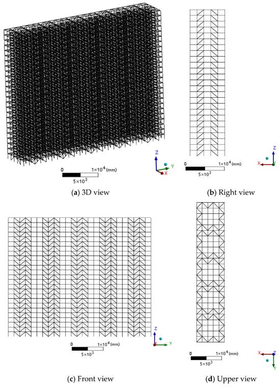
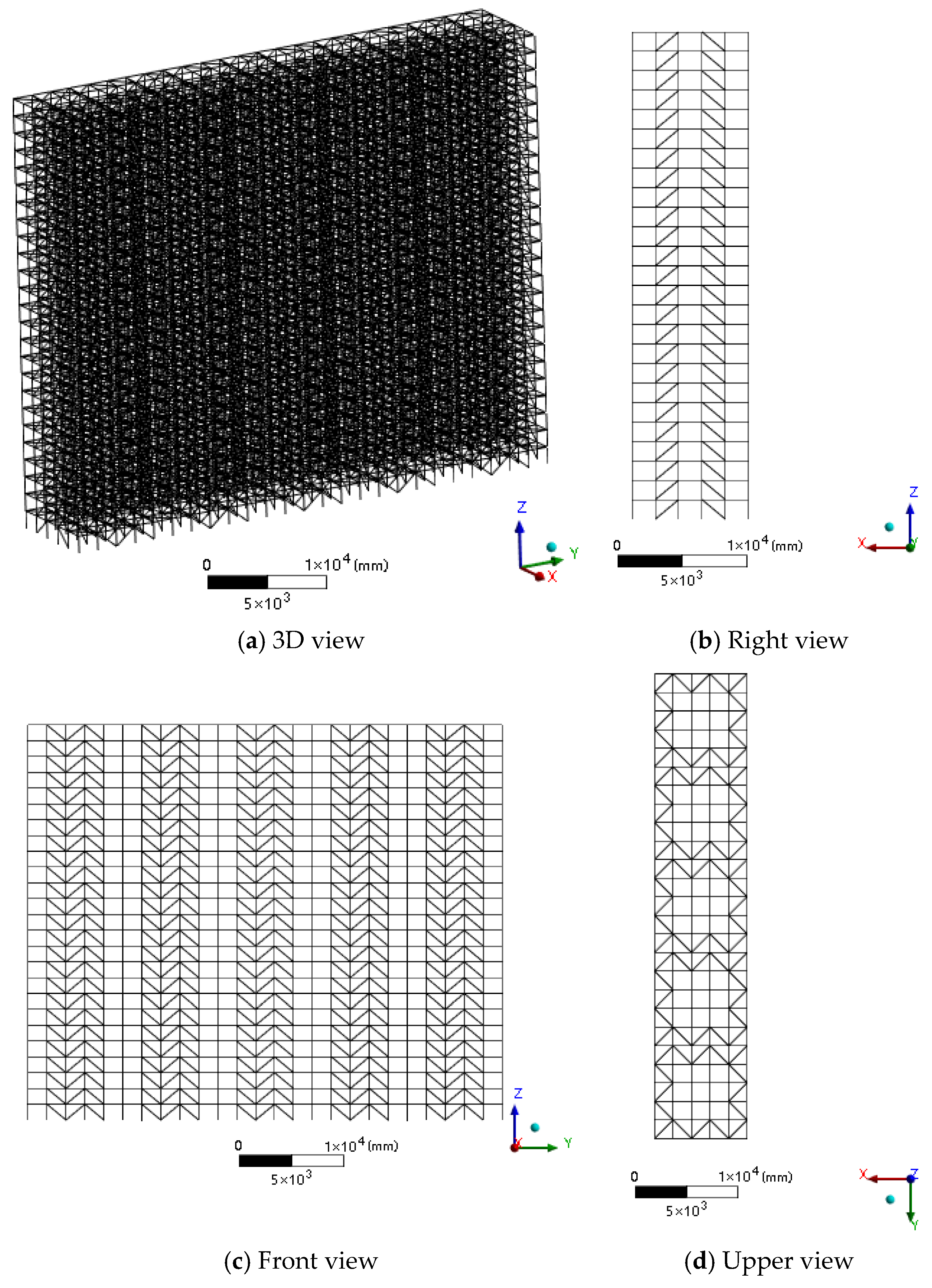
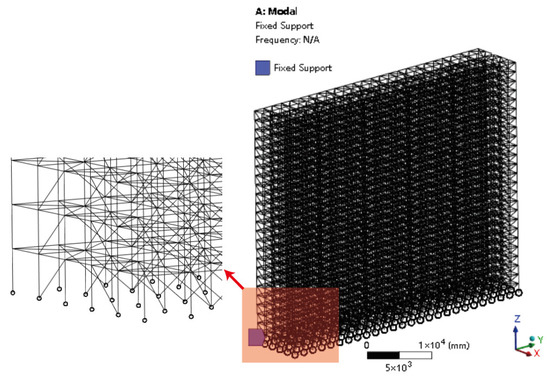
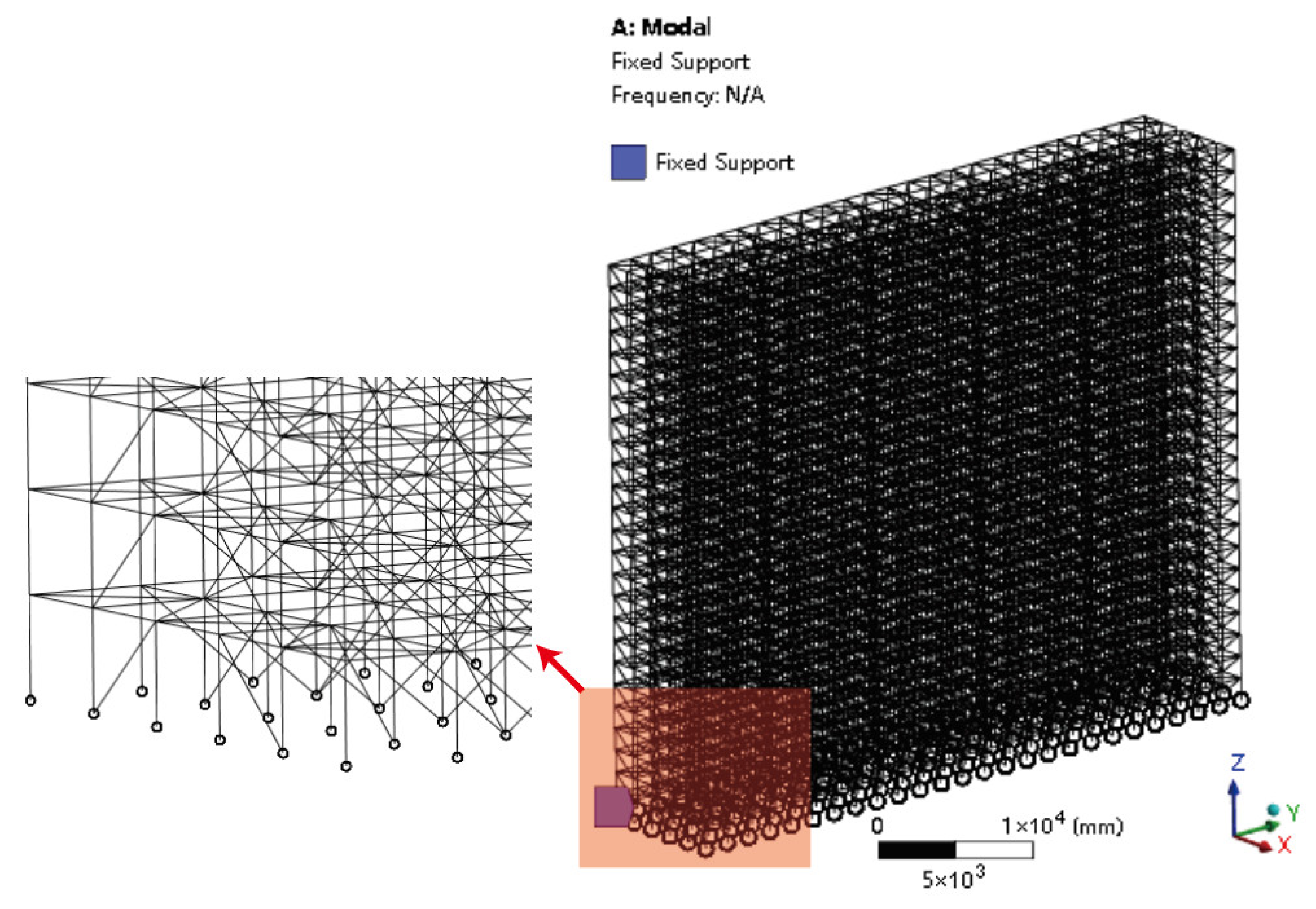
Ansys Workbench software 2023R1 was used to construct FEM of the structural, as shown in Figure 1 [33].

Figure 1. FEM of the large steel frame support structure.

The steel structure employs structural steel, with the member unit type BEAM188. BEAM188 is a 3D 2-node linear Timoshenko beam element with 6 degrees of freedom per node (translations in x, y, z directions and rotations about x, y, z axes). It accounts for transverse shear deformation, making it suitable for the analysis of slender to moderately thick beam structures. This element supports linear analysis, large rotation, and large deformation problems, and can accurately simulate the mechanical behavior of welded and bolted steel frame connections. The specific material parameters are listed in Table 1.

Table 1. Material properties of the large steel frame support structure.

Density (kg/m3)	Modulus of Elasticity (MPa)	Poisson’s Ratio
7850	2 × 105	0.3

3. Numerical Simulation Analysis of the Wind Load

3.1. Governing Equations

In the Cartesian coordinate system for a two-dimensional (2D) unsteady incompressible fluid with constant fluid properties, the governing equations of motion must adhere to the continuity equation and the law of momentum conservation. The corresponding mathematical descriptions are as follows [34,35,36].

Continuity equation: According to the law of mass conservation, the increase in mass within a control volume per unit time should equal the net mass outflow from the control volume during the same time interval. The differential form is expressed as follows:

$${\displaystyle \frac{\partial \rho }{\partial t}}+{\displaystyle \frac{\partial (\rho u)}{\partial x}}+{\displaystyle \frac{\partial (\rho v)}{\partial y}}=0$$

(1)

where u and v are the velocity vectors (m/s) in the x and y directions, respectively. ρ is the density (kg/m³) and t is time (s).

Momentum equation: For a given 2D fluid element, the rate of change in momentum with respect to time should equal the sum of all the external forces acting on the element. The momentum equation essentially satisfies the second law of Newton and is expressed as follows [37,38]:

$$\left.\begin{array}{l}{\displaystyle \frac{\partial \rho u}{\partial t}}+{\displaystyle \frac{\partial \rho uu}{\partial x}}+{\displaystyle \frac{\partial \rho u\nu }{\partial y}}=-{\displaystyle \frac{\partial p}{\partial x}}+{\displaystyle \frac{\partial }{\partial x}}\left[\mu {\displaystyle \frac{\partial u}{\partial x}}\right]+{\displaystyle \frac{\partial }{\partial y}}\left[\mu {\displaystyle \frac{\partial u}{\partial y}}\right]+\mu \left[{\displaystyle \frac{{\partial }^{2}u}{\partial x^2}}+{\displaystyle \frac{{\partial }^{2}v}{\partial y^2}}\right]\\ {\displaystyle \frac{\partial \rho u}{\partial t}}+{\displaystyle \frac{\partial \rho vu}{\partial x}}+{\displaystyle \frac{\partial \rho v\nu }{\partial y}}=-{\displaystyle \frac{\partial p}{\partial y}}+{\displaystyle \frac{\partial }{\partial x}}\left[\mu {\displaystyle \frac{\partial v}{\partial x}}\right]+{\displaystyle \frac{\partial }{\partial y}}\left[\mu {\displaystyle \frac{\partial v}{\partial y}}\right]+\mu \left[{\displaystyle \frac{{\partial }^{2}u}{\partial x^2}}+{\displaystyle \frac{{\partial }^{2}v}{\partial y^2}}\right]\end{array}\right\}$$

(2)

where p represents the pressure on the microelement (N/m²). u and v are the velocity vectors in the x and y directions, respectively (m/s). μ is the viscosity (Pa·s).

The transport equations of the SST (Shear Stress Transport) k-ω model combine the advantages of the SST k-ε turbulence model in the near-wall region and the SST k-ω turbulence model in the far-field region, making it suitable for flow field simulations [39,40]. The core formulas are detailed in the literature [41,42].

3.2. Computational Domain

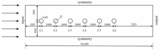
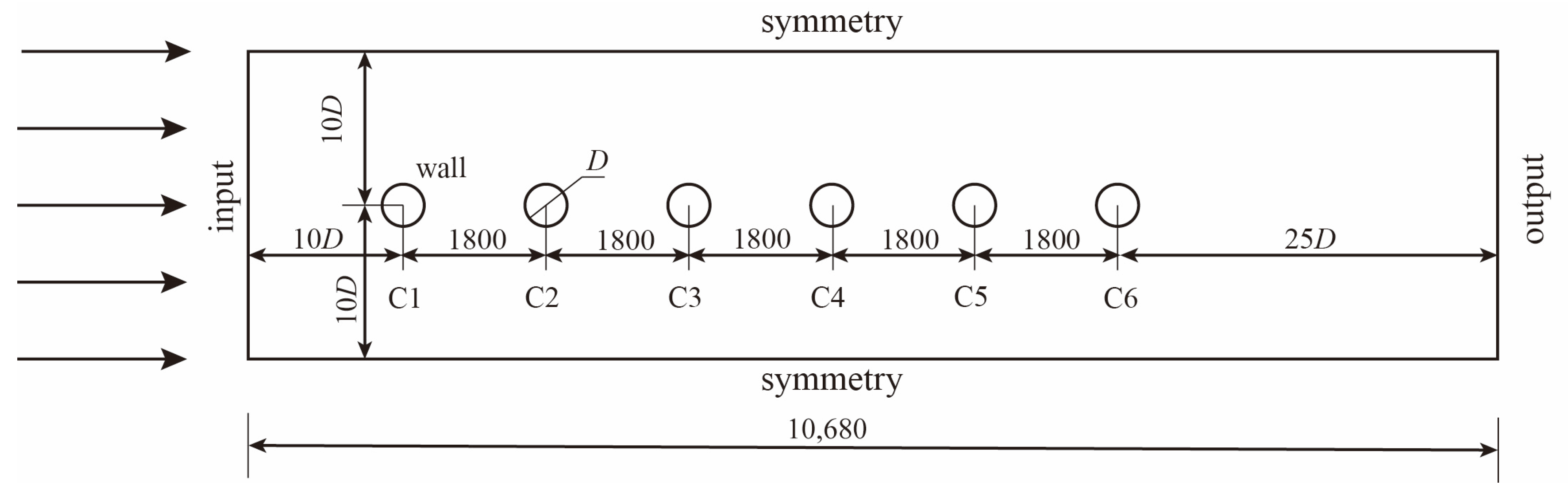
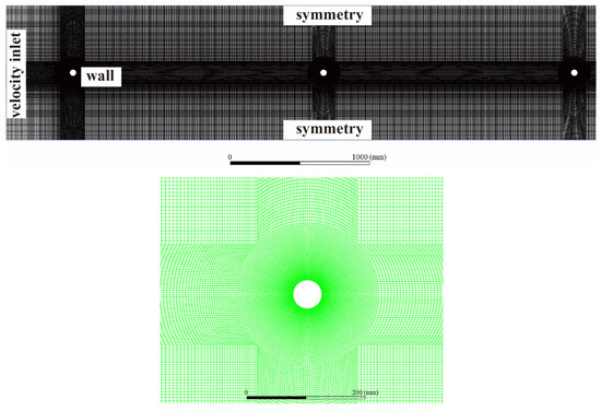
Many researchers have investigated the aerodynamic characteristics of two-and three-dimensional side-by-side cylinders using experimental and numerical methods [43,44,45,46]. Studies have shown that when the spacing ratio L/D of side-by-side cylinders is within 15, the wake patterns, lift, and drag coefficients of the two cylinders are almost identical to those of a single cylinder. Under the working conditions considered in this study, L/D is as high as 31.25. Therefore, the influence of side-by-side cylinders on the lift and drag coefficients is neglected, and only a single column of members is considered. Accordingly, in this study, the CFD simulations involve 2D idealizations of the multirow rod array to obtain the drag coefficients distribution pattern and its spatial variation along the wind direction. Six vertical support rods are selected to simulate and analyze the wind drag of the support structure under wind load. To meet both the computational speed and accuracy requirements, the 2D computational domain is set as shown in Figure 2 based on existing research results [47,48,49]. The total length is 10,680 mm, the width is 20D = 960 mm, the distance from the first rod to the wind velocity inlet is 10D, the distance to both sidewalls is 10D, the spacing between rods is 1800 mm, and the distance from the last rod to the flow field outlet is 25D.

Figure 2. 2D Schematic diagram of the multirow rod computational model.

3.3. Boundary and Initial Conditions

The boundary conditions for the computational domain are set as follows: the inlet adopts a velocity inlet boundary condition, the outlet uses a pressure outlet boundary, the upper and lower boundaries employ symmetric interfaces, and the rods are modeled with no-slip wall boundary conditions. A second-order implicit solver based on pressure-coupled equations is selected, the SIMPLEC algorithm is chosen [50], the SST k-ω turbulence model is applied, and the pressure–velocity coupling uses a second-order upwind scheme. The basic environmental parameters are listed in Table 2.

Table 2. Environmental parameters.

Density (kg/m3)	Dynamic Viscosity (kg/m·s)	Kinematic Viscosity (m2/s)
1.205	1.81 × 10−5	1.506 × 10−5

3.4. Mesh Division and Independence Validation

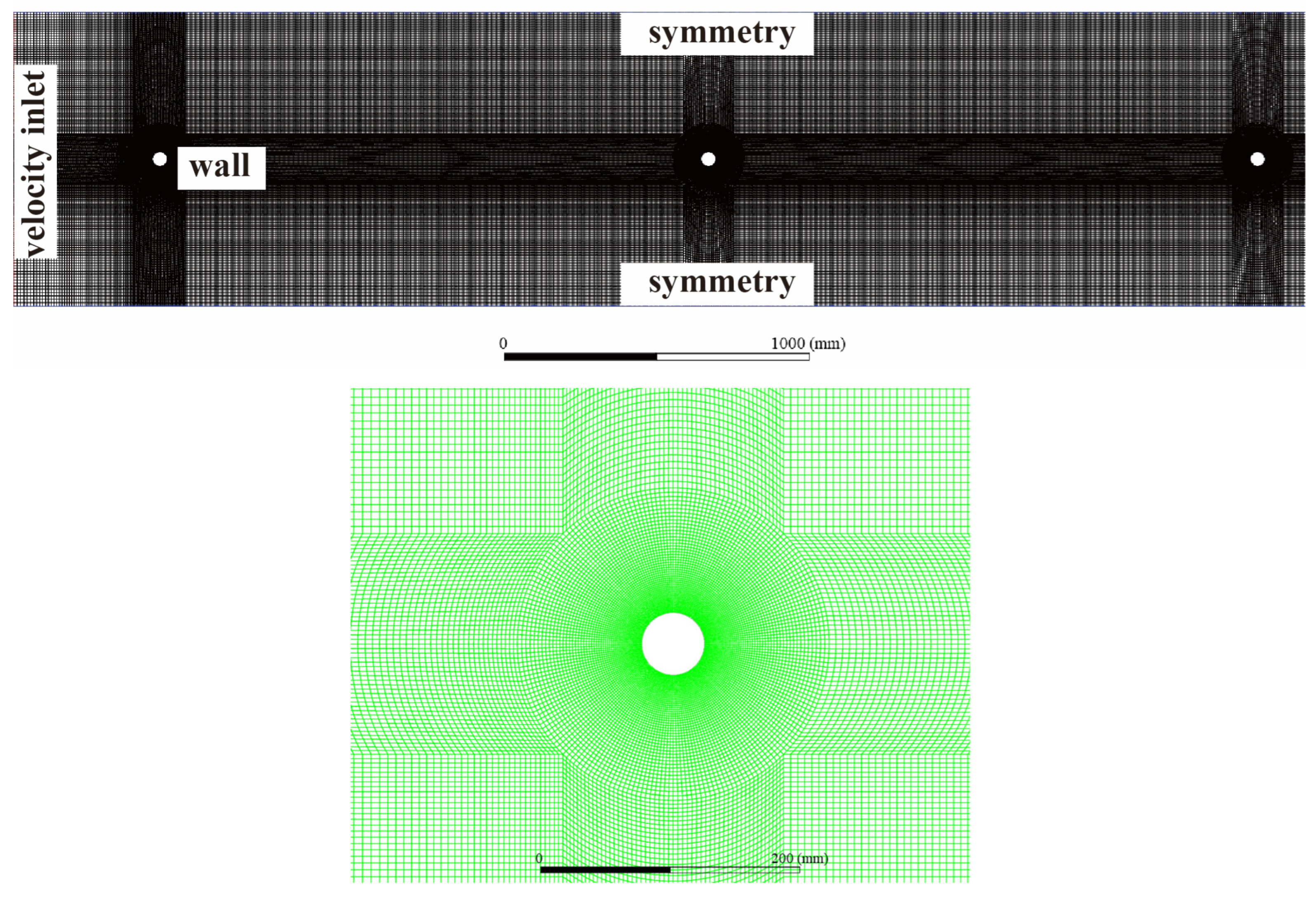
The quadrilateral structured mesh method is adopted for mesh division in this study [51]. The wall function method is used to refine the mesh near the wall surfaces of the rods, with a linear growth rate of 1.1. The first boundary layer mesh size $\mathrm{\Delta }y$ is controlled by ensuring that $y^{+}$≤ 1, which is a dimensionless quantity that describes the normal distance to the physical wall, as calculated via Equations (3) and (4).

$$y^{+}=0.172{\displaystyle \frac{\mathrm{\Delta }y}{l}}R{e}^{0.9}$$

(3)

$$Re=\rho vD/\mu$$

(4)

where Re represents the Reynolds number. l represents the flow field characteristic length. μ represents the air viscosity coefficient. ρ represents the fluid velocity. v represents the free-stream velocity and D represents the cylinder diameter.

To better capture the flow field in the boundary layer, the wake region behind the rods is also refined. The mesh gradually coarsens in areas farther from the rods to reduce the number of mesh elements, balancing computational accuracy and efficiency. The mesh division of the fluid is shown in Figure 3.

Figure 3. Mesh division of the fluid.

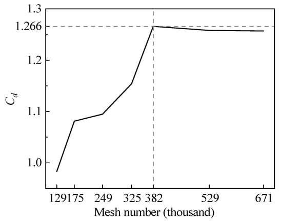
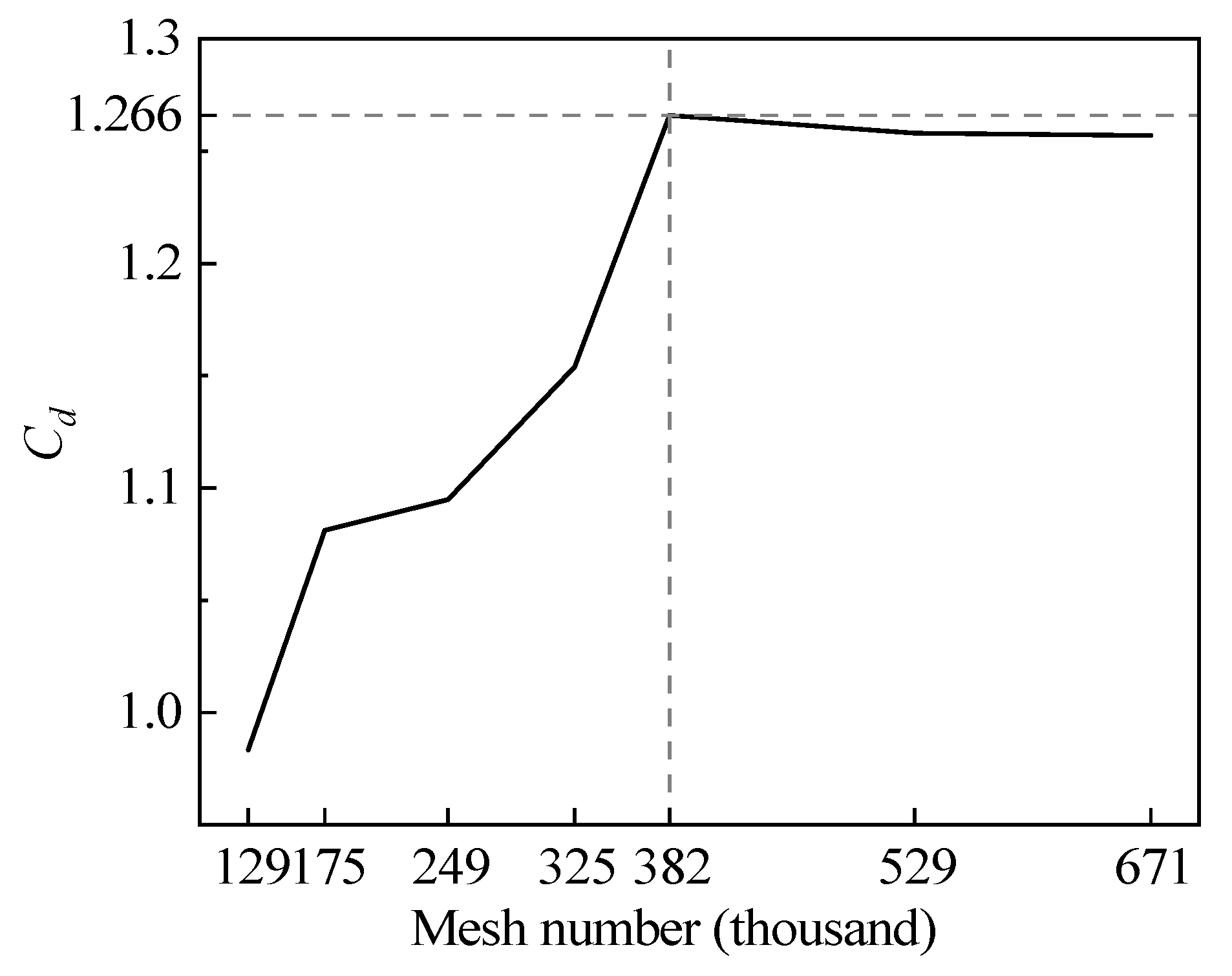
Simulations are conducted using structured mesh elements with varying densities to investigate the influence of the mesh count on the computed drag coefficients of the rod members. The results are compared and validated against existing literature, as detailed in Section 3.5. Validation is specifically performed for the drag coefficient of the first-row rod members at a wind speed of 1.15 m/s. The detailed computational results are presented in Figure 4.

Figure 4. Mesh independence validation.

When the mesh number reached 382 thousand, the computational results exhibited minimal variation. At this stage, the mesh had 168 uniformly distributed nodes in the circumferential direction of the rod members and 42 layers of mesh elements near the wall. Additionally, calculations under a maximum simulated wind speed of 30 m/s with 382 thousand mesh elements yielded a near-wall mesh size $y^{+}$ value of approximately 0.25, which is less than 1, meeting computational requirements. Therefore, the 382 thousand mesh elements were adopted for simulation analysis.

3.5. Verification of Mesh Reliability

To verify the mesh independence, in the present study, the drag coefficients C_d, the root mean square of the lift coefficient C_lrms, and the Strouhal number St of the vertical rod under wind loads with different mesh sizes at a wind speed of 1.15 m/s and Reynolds number Re = 3900 are computed using a time step Δt = 0.005 s. The numerical results are compared with available experimental and numerical data under comparable conditions. Owing to the lack of references for six rods in tandem, this study compares the drag coefficient C_d, root mean square of the lift coefficient C_lrms, and Strouhal number St of the first row of rods with the literature results, as shown in Table 3.

Table 3. Comparison of the numerically simulated results in the present study with the results of similar working conditions in the literature.

Data Sources	Re	Cd	Clrms	St
Experimental results given by reference [52,53]	3900	0.98–1.07	0.25	0.21–0.22
Numerical results given by reference [45,54,55,56,57]	3900	0.99–1.63	0.051–0.316	0.202–0.223
Simulated results in the present study	3900	1.266	0.275	0.214

The results indicate that the differences in the calculations are small. Strouhal number St in the present numerical study is equal to 0.214. This is in fair agreement with existing experimental and numerical data in the range from 0.202–0.223, thereby validating the accuracy and reliability of the adopted numerical model and methodology [57].

3.6. Wind Load Simulation Results and Analysis

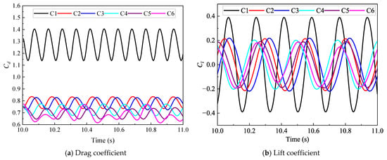
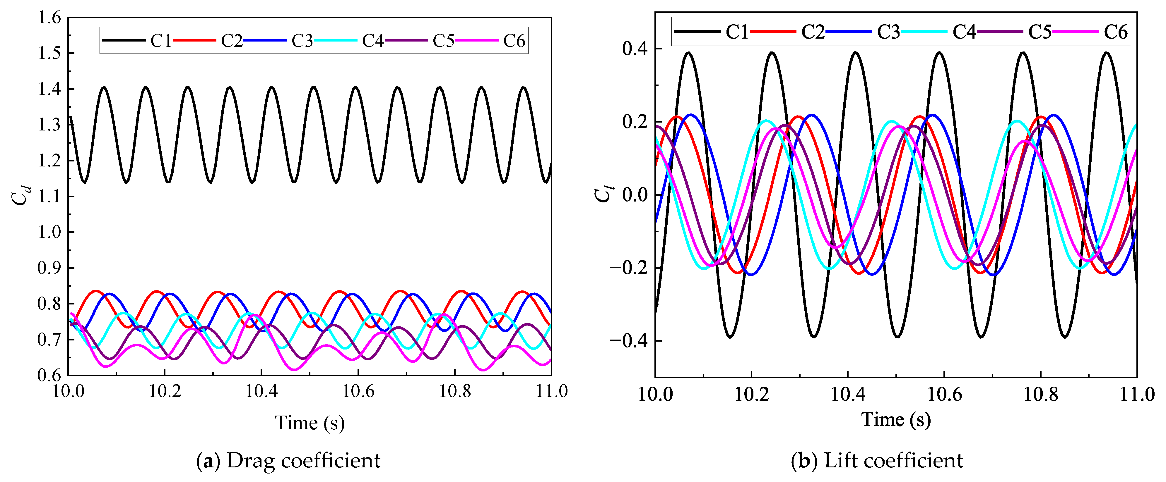
Taking the Reynolds number Re = 3900 as an example, where the wind speed is approximately 1.15 m/s, the variations in the lift and drag coefficients for the members are analyzed. The time–history curves of the lift and drag coefficients for different members at the stable flow stage when Re = 3900 are shown in Figure 5.

Figure 5. Lift and drag coefficients of the structure at Re = 3900.

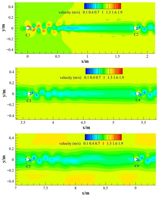
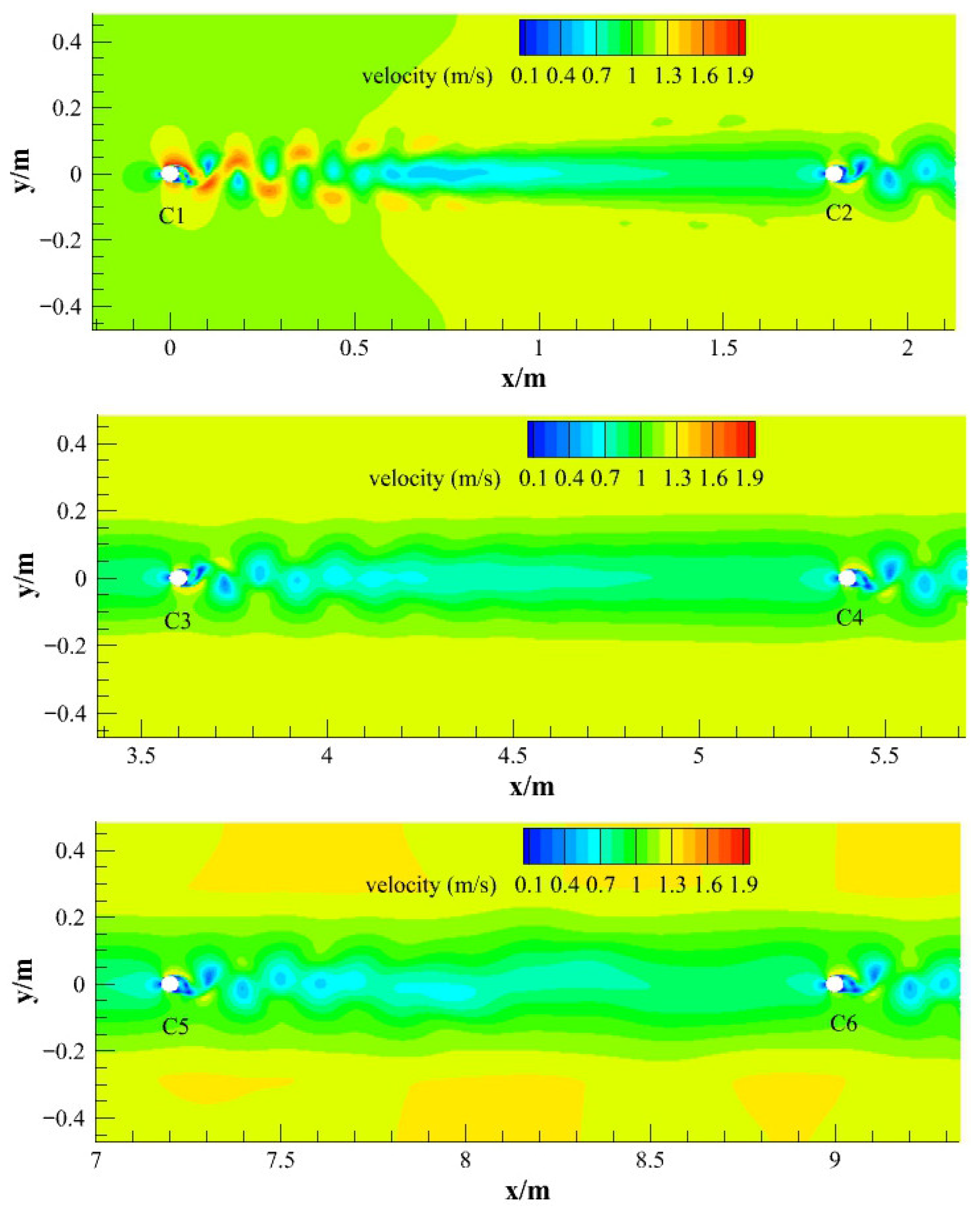
The entire vortex shedding process is stable, with both the lift and drag coefficients displaying periodic variations. The first-row member (C1) has larger amplitudes and relatively stable fluctuation frequencies, where periodic vortex shedding leads to periodic changes in the lift and drag forces. The downstream members (C2–C6) exhibit smaller amplitudes, indicating that they are within the wake of the upstream members. Their own vortex shedding is disturbed and suppressed, resulting in a significant reduction in the oscillation intensity of the lift and drag coefficients. Additionally, the vibration phase of the curves differs markedly from that of the first-row member C1, which is also evident in Figure 6 and Figure 7.

Figure 6. Velocity distribution of the structure flow field at Re = 3900.

Figure 7. Turbulent kinetic energy (TKE) diagram of the structure at Re = 3900.

The velocity distribution of the flow field in the X direction of the support structure at a Reynolds number of Re = 3900 is shown in Figure 6.

The wake pattern behind the members exhibits a shedding mode. After the fluid separates behind each member, vortices form and shed, creating two stable rows of vortex streets. Weak vortex structures appear at the edges of the upstream flow field wake, and their intensity gradually decreases. However, they still influence the vortex shedding of the downstream members. Owing to being within the affected region of the upstream wake, the vortex shedding of the downstream members is suppressed, resulting in relatively weak vortex shedding in their wakes. Overall, because the spacing between adjacent members is large, the wake of the upstream members is almost unaffected by the downstream members, and the acceleration effect of the shear layer behind them is more pronounced. In contrast, the acceleration effect of the shear layer below the downstream members gradually weakens compared with that of the upstream members, and the vortex guidance near the wall surfaces of the rear members essentially disappears. Additionally, the flow velocity near the wall region is lower, leading to weaker instability in the wall flow.

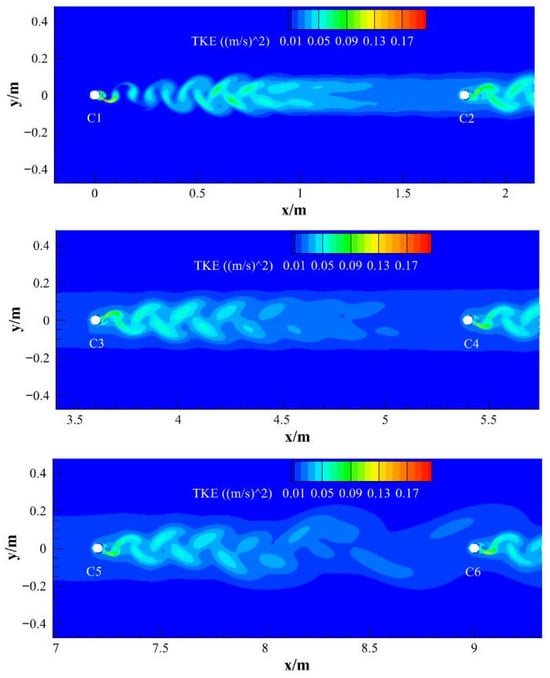
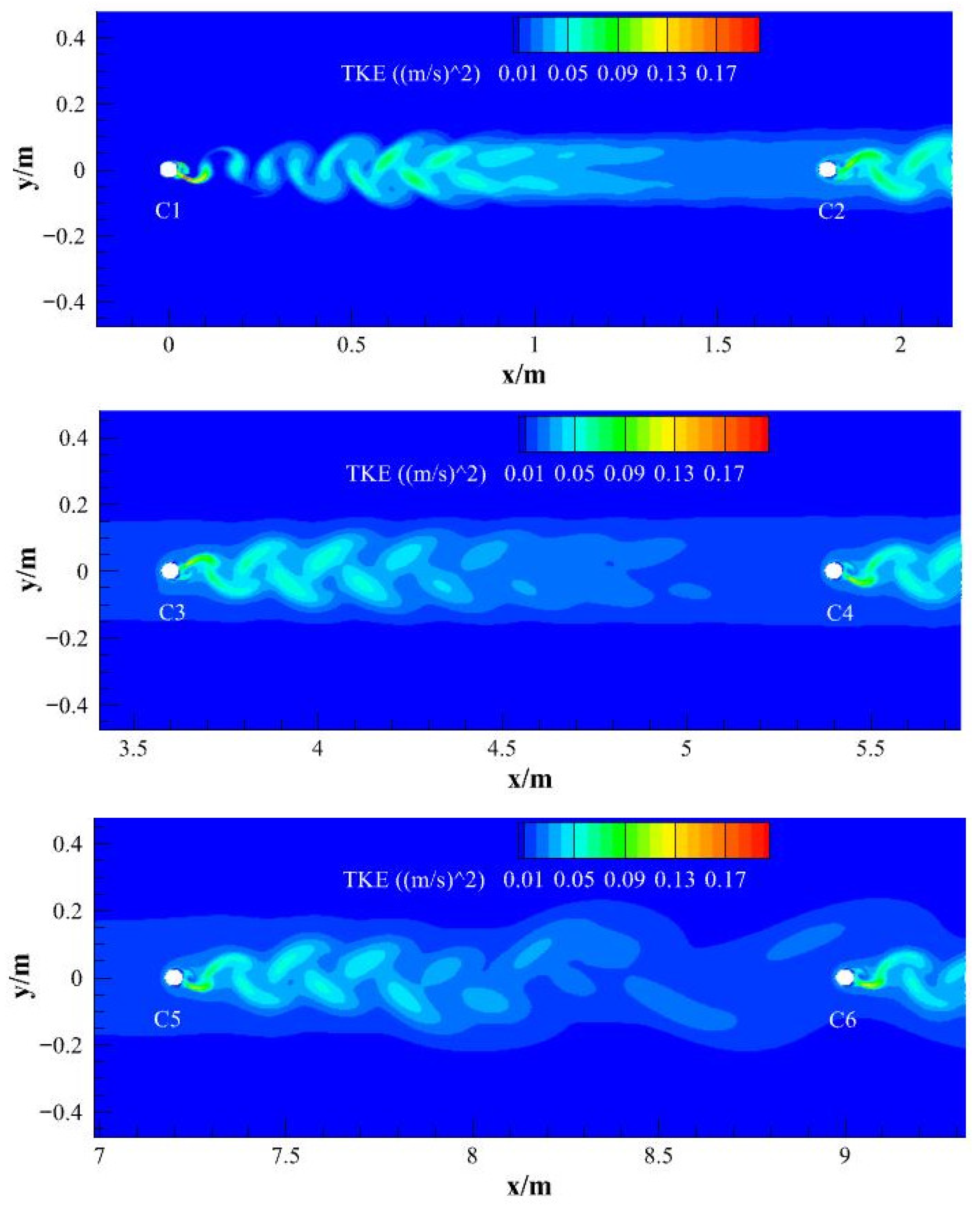
The distribution of the turbulent kinetic energy (TKE) in the flow field is shown in Figure 7.

Since there are no obstructions upstream of C1, a distinct Kármán vortex street (X = 0–1 m) appears behind member C1, characterized by alternating vortices. This region has high TKE values, generating intense turbulent fluctuations and concentrated kinetic energy. In the area between C1 and C2 (X = 1–1.8 m), the flow gradually stabilized, and the vortices dissipated as they moved downstream, leading to reduced TKE values. In the wake region of C2 (X = 1.8–3.6 m), owing to the obstruction caused by C2, new disturbances are introduced to the incoming flow. However, the TKE values here are lower than those in the wake of C1. This is because the incoming flow, after being disturbed by C1, experiences altered turbulence characteristics, resulting in reduced vortex intensity and, consequently, a lower drag coefficient. The same behavior is observed in the rear members (X = 3.6–10.68 m), where the TKE values remain low.

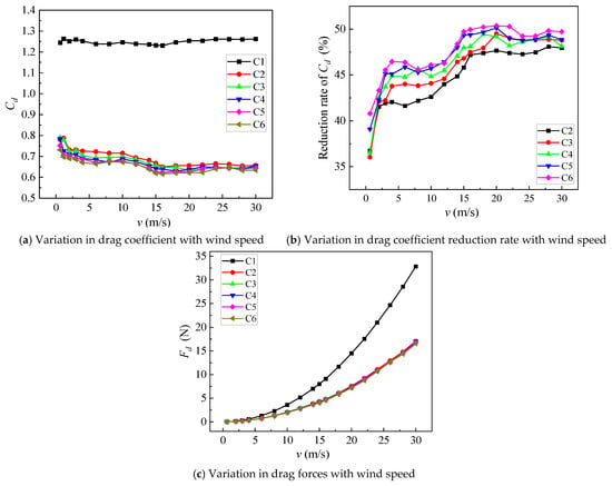
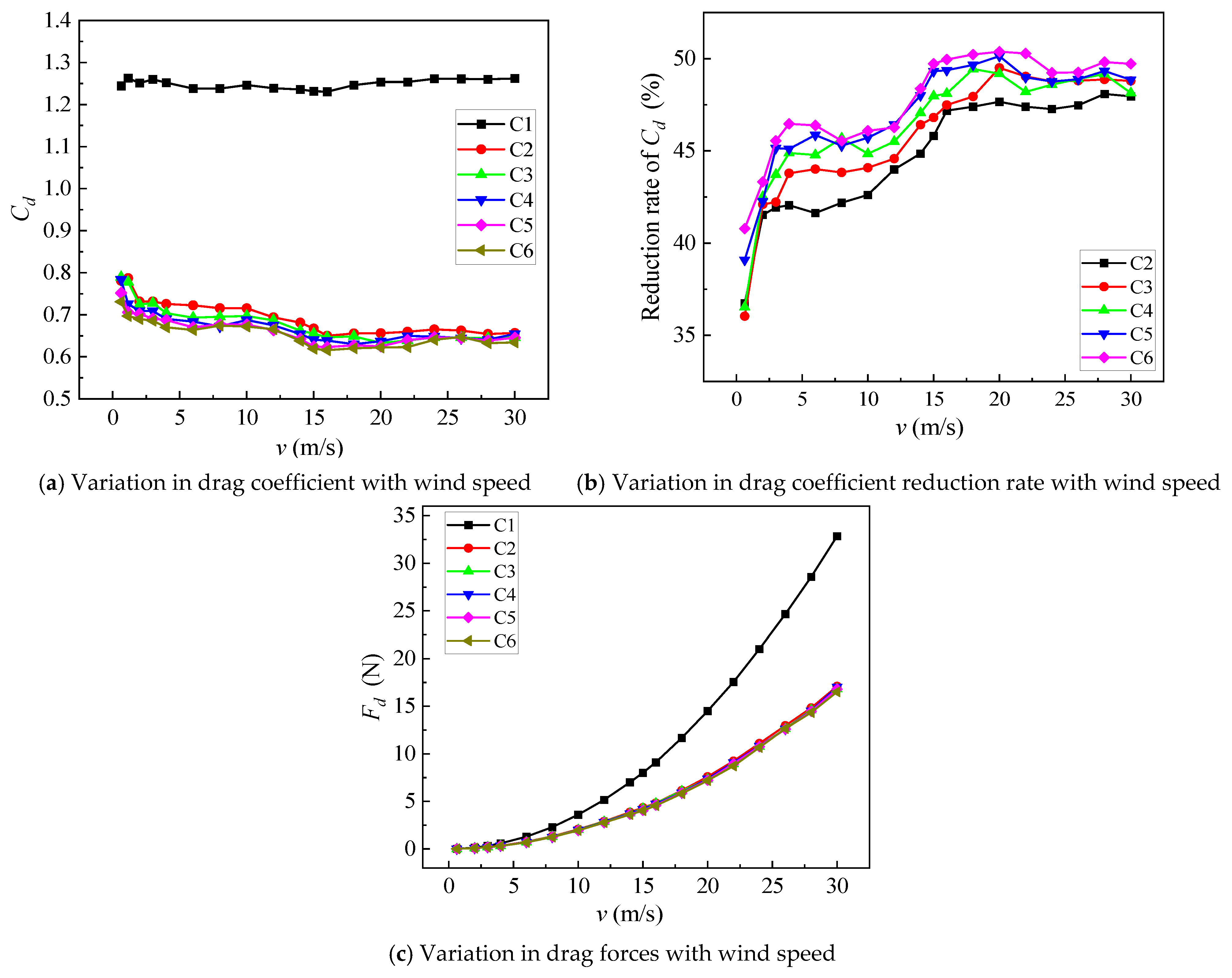
The variations in drag coefficients, drag coefficient reduction rate, and drag force with wind speed are presented in Figure 8a, Figure 8b and Figure 8c, respectively.

Figure 8. Characteristics of drag force variations under different wind speeds.

As shown in Figure 8a, the drag coefficient only slightly changes with increasing wind speed. The C_d varies by less than 3% for the first-row member, confirming that the Reynolds number is insensitive to the subcritical flow regime. This characteristic is consistent with the established cylindrical aerodynamic theory, where the drag coefficient remains approximately constant for 10³ < Re < 2 × 10⁵ [58]. The drag coefficient of the first row of members fluctuates slightly by approximately 1.25, whereas the drag coefficients of the second and subsequent rows are relatively close, fluctuating between approximately 0.6–0.8, and the drag coefficient tends to decrease further downstream. This is due to the large ratio of the distance between members to their diameter. Shear layers from upstream members roll up into periodically shedding vortices, which envelop the downstream members. The wake resembles that of the flow around a single member, displaying a typical Kármán vortex street with a double-row vortex structure. The flow interference generated by upstream members reduces the drag coefficients of downstream members, as also observed in Figure 6 and Figure 7.

As shown in Figure 8b, The drag coefficient reduction rate increases with increasing wind speed. When the wind speed exceeds 15 m/s, the drag coefficient reduction rate essentially remains constant. Overall, the drag coefficient reduction rate increases with increasing downstream position of the members.

As shown in Figure 8c, the drag force acting on the members increases gradually with increasing wind speed, following a quadratic growth trend that is consistent with the theoretical formulations. At the same wind speed, the first row of members is subjected to the maximum drag force, whereas the drag forces on the downstream members are relatively comparable.

4. Dynamic Response Analysis of the Structure

4.1. Structural Motion Equation

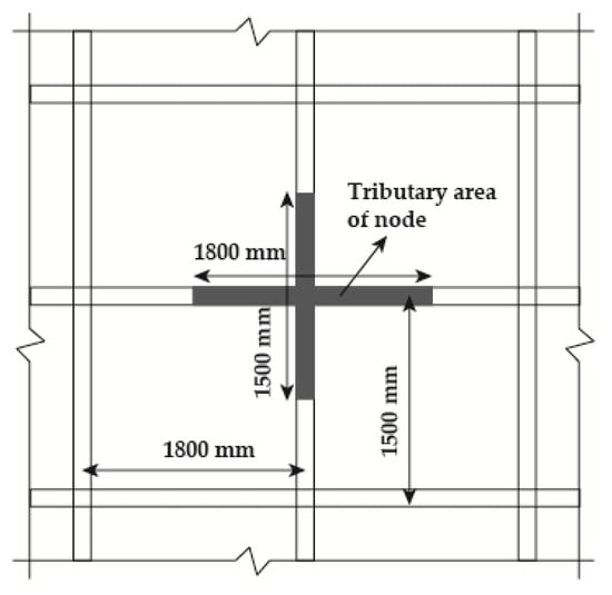
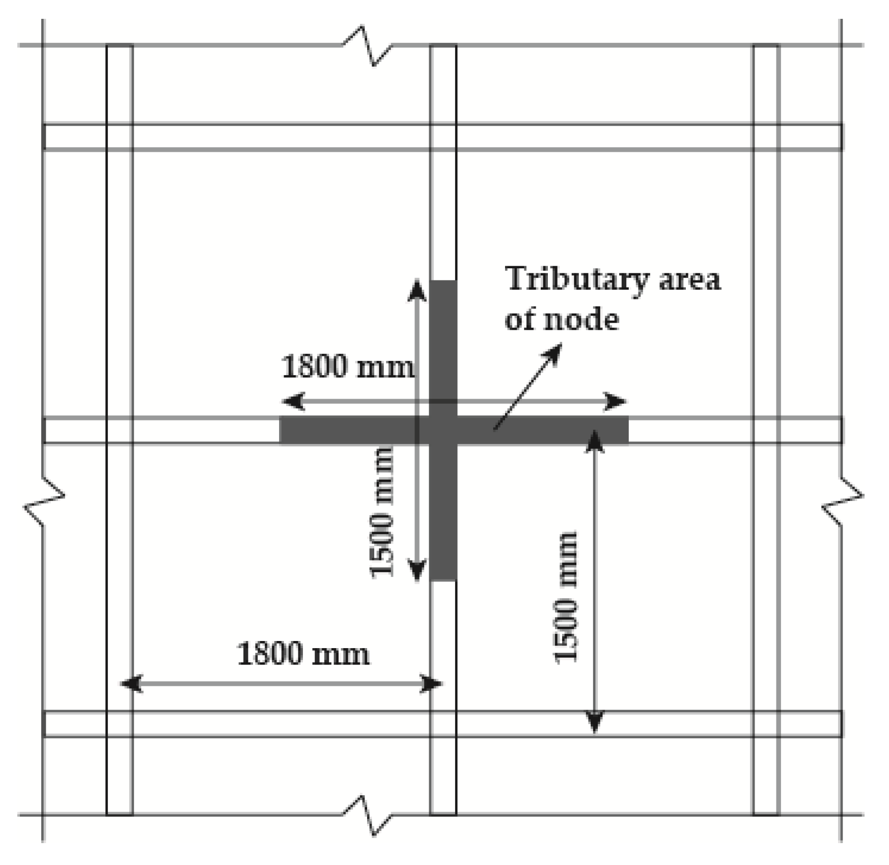
Based on the tributary area of each node and the time–history of the fluctuating drag coefficient obtained from the unsteady flow field simulation, the fluctuating wind force time–history at the nodes of each row of members is determined using Equation (5).

$$F_d={\displaystyle \frac{1}{2}}\rho v^2{C}_{d}DL$$

(5)

where ρ is the air density. $C_d$ is the drag coefficient, v is the wind speed. $F_d$ is the wind load and L is the tributary length based on the structural grid spacing (1500 mm vertically, 1800 mm horizontally).

The fluctuating wind forces are concentrated and applied at each structural node. This mapping procedure is illustrated in the schematic diagram presented in Figure 9.

Figure 9. Schematic diagram of nodal mapping.

The fluctuating drag coefficient time–history is extracted from the final 5 s of the 15 s unsteady CFD simulation (after reaching statistical stationarity), with a sampling time step of Δt = 0.005 s. Each row of vertical members (C1–C6) adopts the identical C_d(t) time–history derived from the corresponding rod in the 2D CFD simulation. Independent time-histories are assigned to different rows to reflect their relative positions in the wake, with the phase differences between rows neglected. Owing to the relatively low height of the structure (37.5 m), the relatively compact footprint of the structure and the global correlation of wind gusts is high, the variations in the wind load along the structural height is neglected.

Based on the dynamic equilibrium equation of the large steel frame support structures under seismic excitation alone, the equation of motion for the structure under combined earthquake–wind action is given in Equation (6) [59].

$$M\ddot{X}+C\dot{X}+KX=M{\ddot{X}}_g+F_{\mathrm{d}}$$

(6)

4.2. Model Establishment and Boundary Conditions of the Structure

The FEM of the structure is a fully anchored temporary support (e.g., those for LED screens at large-scale events). The connections of the FEM between the primary structural members (beams and columns) are idealized as rigid connections, reflecting the typical welded or heavily bolted joints of such systems, while the column bases are modeled as fixed supports. Furthermore, the selected structural dimensions (45 m × 9 m × 37.5 m) and the corresponding slenderness ratios are highly representative of standard configurations used for large-scale temporary logistics hubs and industrial support towers. The layout of the cross-bracing system aligns with standard engineering practices, ensuring that the dynamic characteristics (e.g., translation–torsion coupled modes) derived from this model accurately reflect actual field behaviors.

In this study, linear elastic analysis is adopted to clearly reveal the dynamic superposition effect of earthquake–wind coupling actions, so as to avoid additional variables introduced by nonlinearity from obscuring the coupling mechanism. To verify the influence of geometric nonlinearity on the structural vibration amplitude, some parametric checks were conducted. The results show that the difference caused by geometric linearity or nonlinearity is approximately 3%. Therefore, the effect of geometric nonlinearity on the vibration amplitude lies within the acceptable error range. To improve computational efficiency, linear analysis is adopted in this study.

The large steel frame support structure model uses structural steel, and the member unit type is BEAM188. The calculation model is shown in Figure 10.

Figure 10. FEM of the structure.

4.3. Modal Analysis

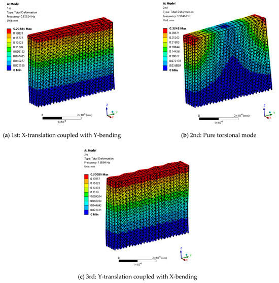
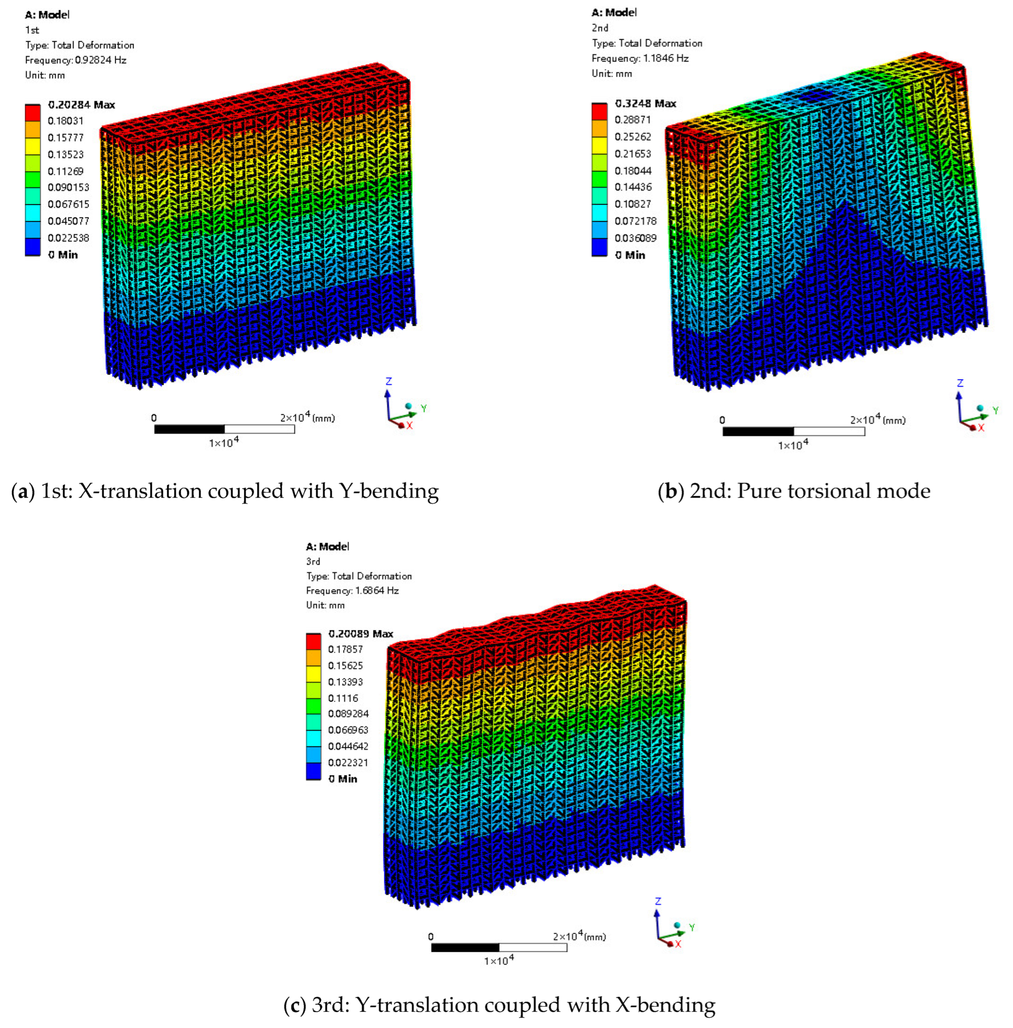
Modal analysis is performed to identify the vibration modes and natural periods of the structure. The periods and Modal Participating Mass Ratios (MPMRs) of the first six vibration modes of the model are presented in Table 4. Mode shape diagrams for the first four modes are presented in Figure 11.

Table 4. Results of modal analysis.

Mode	Period (s)	MPMR (%)						Dominant Actual Mode Characteristic
		X	Y	Z	X-Bending	Y-Bending	TOR-Z
1st	1.08	65.30	0.04	0.00	0.06	93.15	39.63	X-translation coupled with Y-bending
2nd	0.84	0.05	0.00	0.00	0.00	0.00	23.54	Pure torsion around the vertical axis
3rd	0.59	0.05	63.81	0.00	47.33	0.00	2.90	Y-translation coupled with X-bending
4th	0.24	17.24	0.01	0.00	0.00	1.07	10.32	Higher-order X-translation
5th	0.21	0.02	0.00	0.00	0.00	0.00	5.71	Higher-order torsion around the vertical axis
6th	0.13	0.00	19.87	0.04	1.01	0.00	0.75	Higher-order Y-translation

Figure 11. Mode shape diagrams for the first three modes.

The first three modes of the structure are characterized by global vibration. Specifically, the first mode (1.08 s) is dominated by X-direction translation (65.30%) coupled with significant bending about the Y-axis (93.15%). The second mode (0.84 s) is a pure torsion mode around the vertical axis (23.54%), while the third mode (0.59 s) is dominated by Y-direction translation (63.81%) coupled with X-direction bending (47.33%). The significantly longer period of the first mode compared to the third indicates that the structural stiffness in the X-direction is lower than that in the Y-direction. Furthermore, the relatively low global bending stiffness results in pronounced translation–bending coupling effects. The fourth to sixth modes correspond to higher-order vibrations, namely higher-order X-direction translation (17.24%), higher-order torsion around the vertical axis (5.71%), and higher-order Y-direction translation (19.87%). Given their relatively small modal participating mass ratios, these higher-order modes contribute minimally to the overall dynamic response of the structure.

4.4. Selection of Seismic Waves

In this study, the seismic design group is the second group, the site is Class II, the characteristic period T_g is 0.4 s, the damping ratio ξ = 0.02, the seismic fortification intensity is 7 degrees, the basic design acceleration is 0.2 g, and the target response spectrum is obtained according to the design response spectrum specified in the Chinese seismic design code (GB50011-2010) [60].

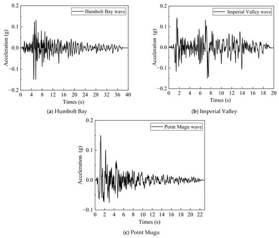
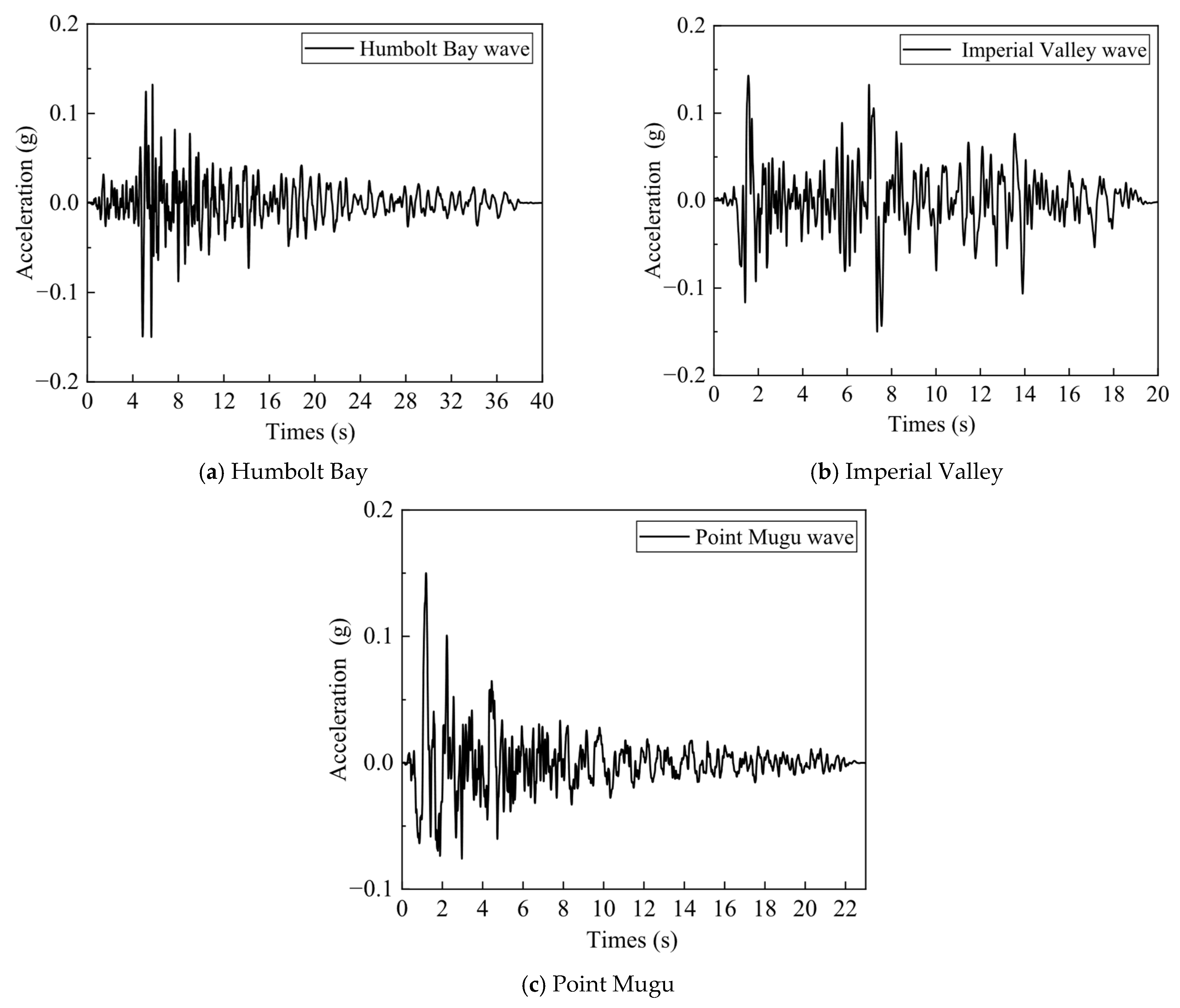
To meet the requirements of the Chinese seismic design code (GB50011-2010) [60], when the time–history analysis method is adopted, acceleration time–history curves should be selected based on the site category and design earthquake group, with the number of actual earthquake records not less than two-thirds of the total. To accurately capture real-world seismic characteristics, three sets of actual ground motion records are chosen for analysis. The selection process prioritized the matching of the response spectra with the design spectrum of Site Class II, ensuring the frequency-domain characteristics of the seismic input were representative of the design requirements. Three real ground motion acceleration time–history curves are selected from the Pacific Earthquake Engineering Research Center (PEER) database: Humbolt Bay (1937), Imperial Valley (1953) and Point Mugu (1973) [61].

To balance computational efficiency with accuracy and considering that the peak ground acceleration of the selected seismic waves is contained within the first 15 s, only the first 15 s of each seismic wave containing the peak ground acceleration are selected as the ground input for the supporting structure [62]. In accordance with the research requirements of this study, the original seismic wave curves are scaled to 0.05 g, 0.10 g, 0.15 g, and 0.20 g using the PGA scaling method. Specifically, the selected ground motion records were scaled in terms of peak ground acceleration (PGA) to match the target fortification intensities. The acceleration time–history curves scaled to 0.15 g are shown in Figure 12.

Figure 12. Seismic wave time–history curves.

In this study, the seismic ground motions were applied unidirectionally along the transverse direction of the structure (X-direction), as this short-axis orientation represents the most critical and vulnerable direction for dynamic excitation due to the highly asymmetric plan of the support system.

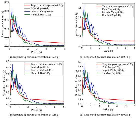
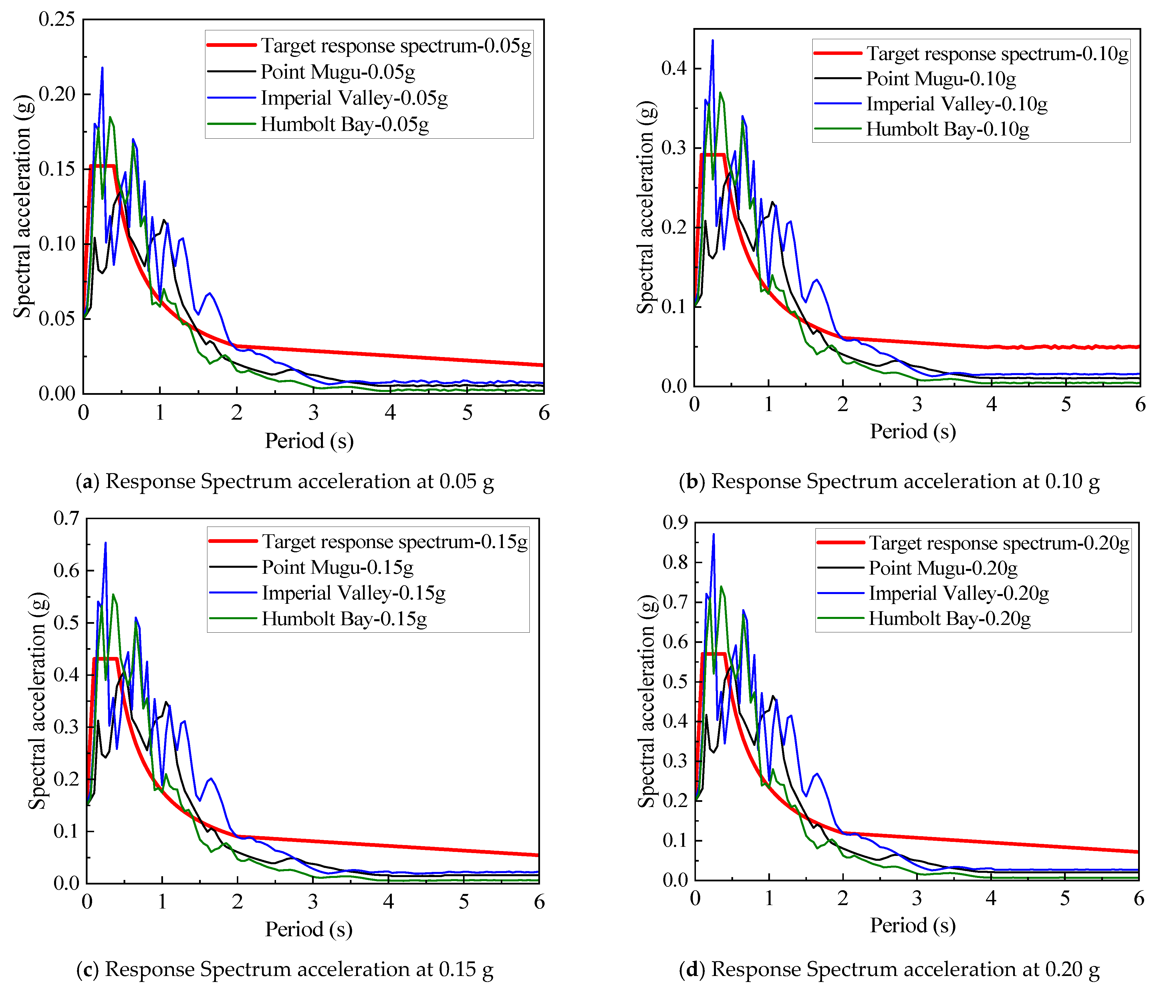
A comparison of the scaled ground motion response spectra with the target design spectrum at PGA levels of (a) 0.05 g, (b) 0.10 g, (c) 0.15 g, and (d) 0.20 g is shown in Figure 13.

Figure 13. Comparison of scaled ground motion response spectra with the target design spectrum at PGA levels of (a) 0.05 g, (b) 0.10 g, (c) 0.15 g, and (d) 0.20 g.

The deviation between the mean value of the seismic records and the standard response spectra is within 20% in the period range of 0.2 T–2.0 T (0.22–2.2 s, covering the structure’s fundamental period of 1.08 s), which can be used for time–history analysis [63].

4.5. Vibration Responses of the Structure Under Different Seismic Actions

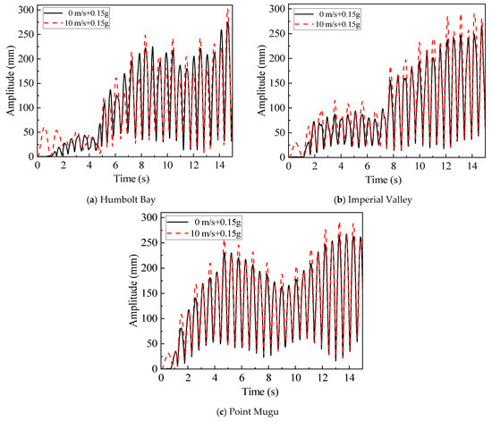
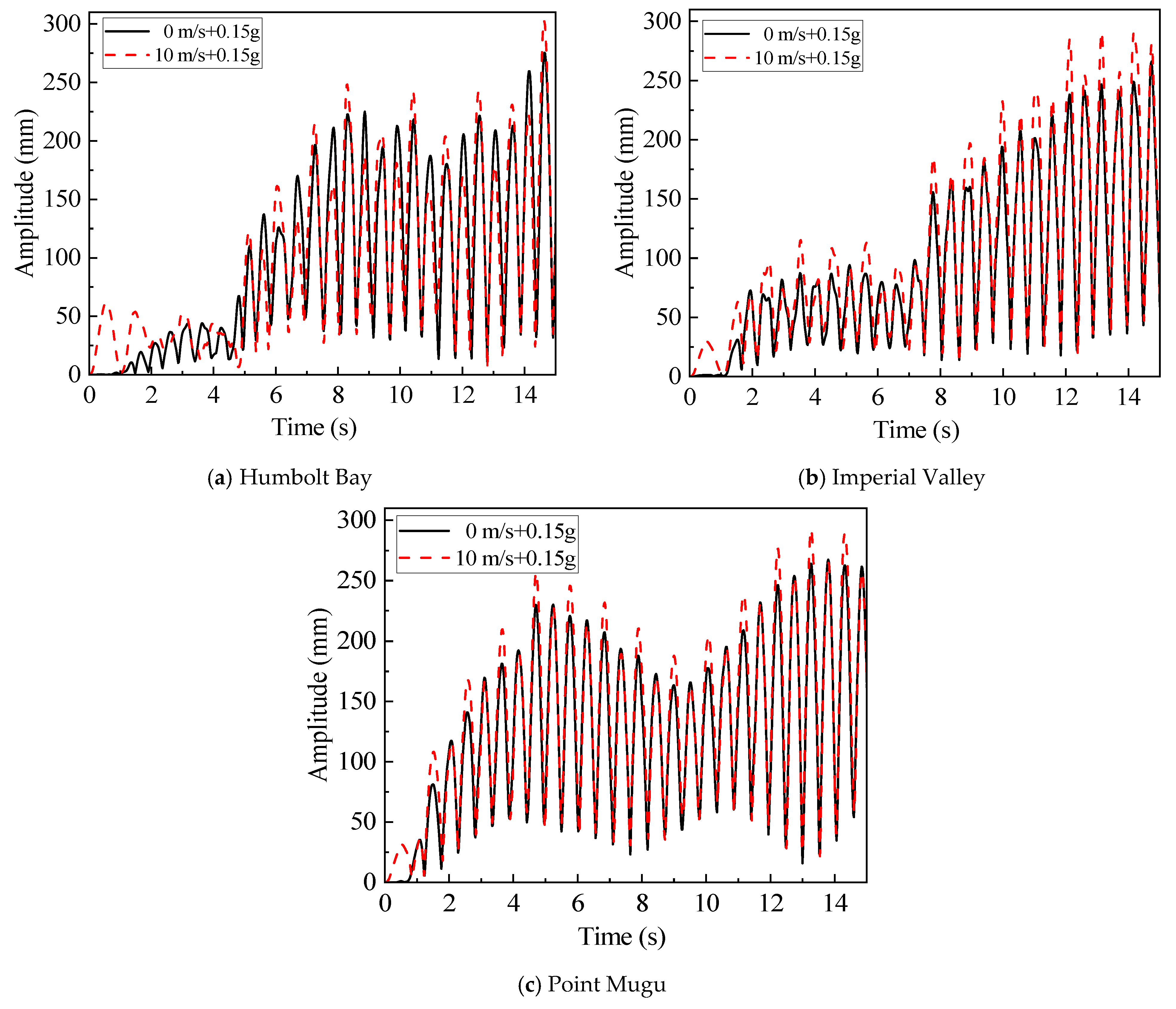
In this study, the dynamic behavior of the large steel frame support structure is evaluated under combined hazard scenarios. Three sets of seismic waves and wind loads with wind speeds of 0 m/s and 10 m/s are applied to the structure. The 10 m/s wind speed is selected here as a representative case to illustrate the dynamic coupling characteristics, as consistent response trends were observed at higher wind speeds. A dynamic time–history analysis is carried out along the transverse direction of the short side (X-direction) of the structure to obtain the structural displacement time–history curves. The displacement responses are specifically extracted from the nodes at the top chord of the steel frame, where the maximum lateral drift is expected to occur. The resulting displacement time–history curves are shown in Figure 14. Furthermore, the spatial deformation characteristics observed in the time–history analysis remain consistent with the fundamental mode shapes described in Figure 11.

Figure 14. Structural amplitude under different seismic waves when the wind speed is 0 and 10 m/s.

The results indicate that under the action of Humbolt Bay, Imperial Valley and Point Mugu seismic waves, the maximum displacement amplitudes of the structure are 275 mm, 266 mm, and 267 mm, respectively. Under the combined actions of three types of 7-degree seismic forces (0.15 g) and a wind speed of 10 m/s, the maximum displacement amplitudes of structural vibration are 302 mm, 290 mm, and 293 mm, respectively. Under the influence of wind, the structural vibration amplitudes increase compared with those without wind, with increase ratios of 9.7%, 9.0%, and 9.6%, respectively. A comparison of Figure 12 and Figure 14 reveals that the maximum structural amplitude occurs in regions corresponding to greater seismic accelerations. Under different seismic waves, the waveforms of the maximum structural amplitudes differ significantly, but the magnitudes of the maximum amplitudes are relatively close.

4.6. Responses of the Structure Under Different Wind Speeds and Seismic Accelerations

To study the amplification effect of the wind load on the structural vibration amplitude, the wind load amplification factor λ is defined. Here, λ reflects the influence of different wind loads on the structural amplitude under a certain seismic acceleration. The calculation formula is shown in Equation (7).

$$\lambda ={\displaystyle \frac{X_{E,W}-X_E}{X_E}}\times 100\%$$

(7)

where $X_{E,W}$ is the vibration amplitude of the support structure under combined wind and seismic actions and where $X_E$ is the vibration amplitude of the support structure under seismic action alone.

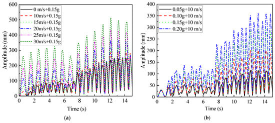
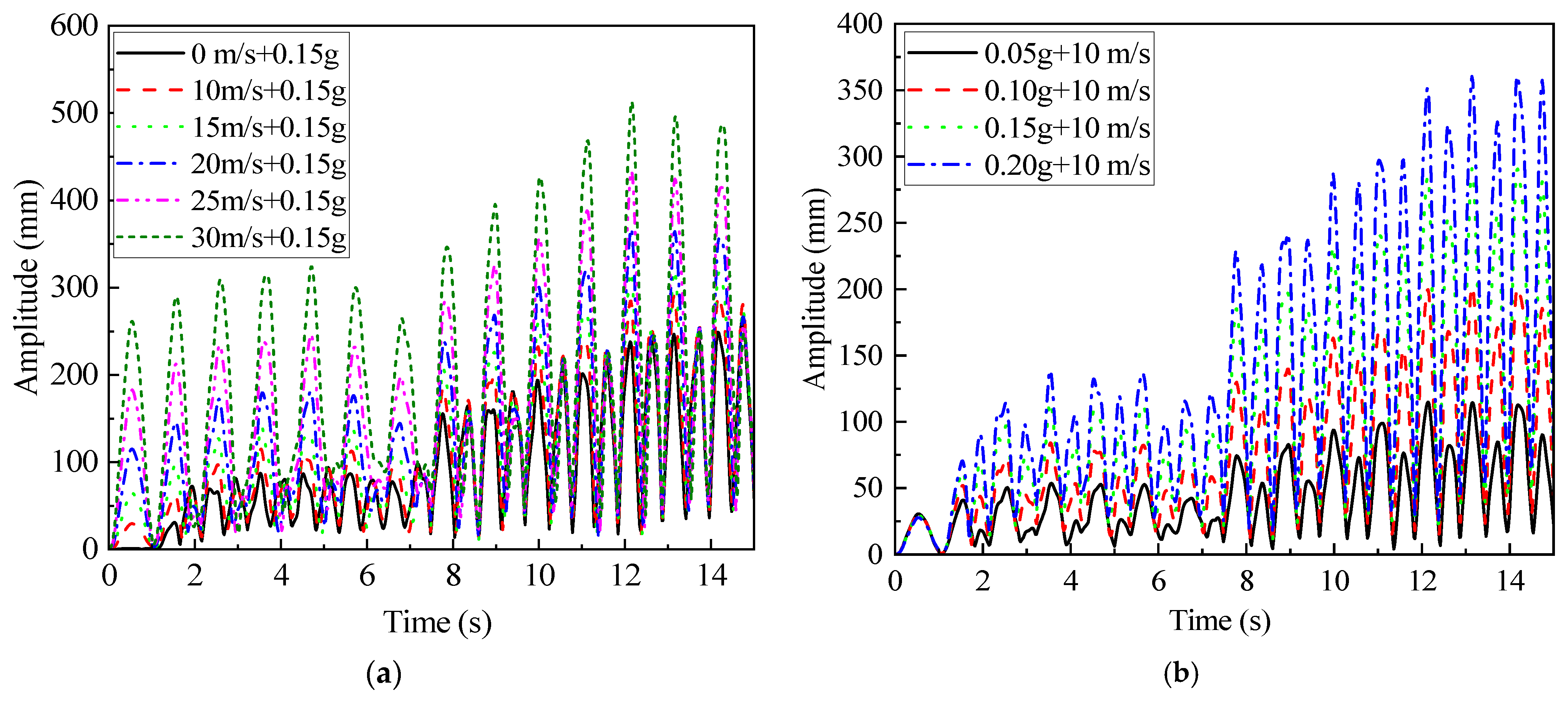
The Imperial Valley seismic wave is selected from the calculation results, and its amplitude is adjusted to obtain maximum amplitudes of 6 degrees (0.05 g), 7 degrees (0.1 g), 7 degrees (0.15 g), and 8 degrees (0.2 g). Wind speeds of 10 m/s, 15 m/s, 20 m/s, 25 m/s, and 30 m/s are subsequently superimposed. The time–history responses of the structural amplitude under combined wind speeds and seismic accelerations are obtained, as illustrated in Figure 15.

Figure 15. Time–history responses of the structural amplitude under different wind speeds and seismic accelerations. (a) Time–history of the structural amplitude under different wind speeds; (b) Time–history of the structural amplitude under different seismic accelerations.

As shown in Figure 15, the linear elastic simulation analysis yields the structural vibration amplitudes under the Imperial Valley seismic wave combined with different wind speeds, thus characterizing the hazard interaction effects.

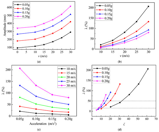
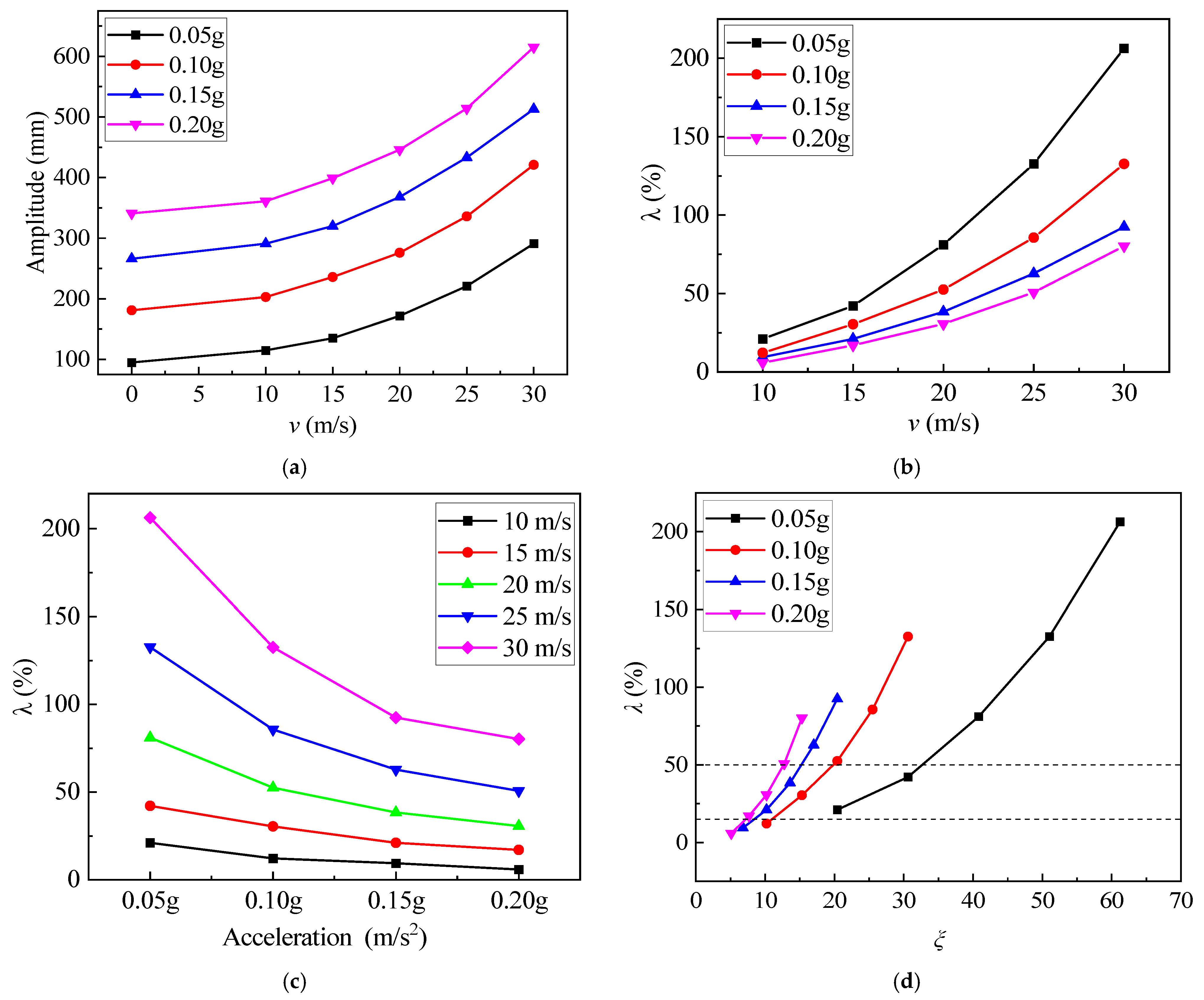
The maximum vibration amplitudes of the structure under different wind speeds and seismic accelerations are shown in Figure 16a. The variation curves of the wind load amplification factor λ under different wind speeds and seismic accelerations are shown in Figure 16b and Figure 16c, respectively. The wind load amplification factor λ under different ξ values is shown in Figure 16d.

Figure 16. Structural amplitude and wind load amplification factor of the structure under different wind speeds and seismic accelerations. (a) Structural amplitude under different wind speeds; (b) Wind load amplification factor under different wind speeds; (c) Wind load amplification factor under different seismic accelerations; (d) Wind load amplification factor under different ξ.

The results indicate that under the action of the Imperial Valley seismic wave, the amplitude of the support structure gradually increases as the wind speed increases. When the wind load and seismic action are combined, under a certain seismic acceleration applied to the structure, the amplifying effect of the wind load on the structural amplitude gradually increases with increasing wind speed. Conversely, when a constant wind speed is applied to the structure, the amplifying effect of seismic acceleration on the structural amplitude gradually decreases as the acceleration increases. Under the working conditions studied in this study, when the seismic acceleration is at its minimum of 6 degrees (0.05 g) and the wind speed reaches its maximum of 30 m/s, the combined effect results in the maximum amplifying effect of the wind load on the structural amplitude at 206.3%.

The wind-dominated regime is defined as the condition where the wind load amplification factor λ > 50%, the earthquake-dominated regime is defined as λ < 15%, and the range of 15% ≤ λ ≤ 50% is defined as the transition zone of load dominance. For the structural configuration investigated in this study, a practical engineering design criterion is proposed based on the velocity-to-acceleration ratio ξ, the calculation formula is shown in Equation (8).

$$\xi ={\displaystyle \frac{velocity}{acceleration}}$$

(8)

The wind load amplification factor λ under different ξ values is shown in Figure 16d, from which the specific judgment criteria for different seismic intensities are derived as follows:

• 6 degree (0.05 g): earthquake-dominated for ξ < 18 and wind-dominated for ξ > 33;
• 7 degree (0.10 g): earthquake-dominated for ξ < 10 and wind-dominated for ξ > 20;
• 7 degree (0.15 g): earthquake-dominated for ξ < 8 and wind-dominated for ξ > 15;
• 8 degree (0.20 g): earthquake-dominated for ξ < 7 and wind-dominated for ξ > 12;

This ratio can be calculated at the preliminary design stage by combining site-specific wind speed data and seismic hazard maps. The ξ threshold parameters proposed in this study are calibrated for the specific structural configuration analyzed (structural height 37.5 m, natural period 1.08 s, damping ratio 2%, fully anchored support). For structures with significantly different dynamic characteristics (e.g., tall support structures with longer natural periods that are closer to the peak of the wind load energy spectrum), the ξ thresholds need to be recalibrated.

4.7. Discussion and Limitations

While this study establishes a systematic framework for multihazard dynamic analysis, several limitations should be acknowledged to define the boundaries of the current findings:

(1)

Material Linearity: The current structural model is strictly linear-elastic. While this approach effectively isolates the fundamental ‘load-dominance transition’ mechanism without the interference of complex hysteretic variables, it neglects material nonlinearity and energy dissipation. Future studies should incorporate elastic-plastic models to assess the ultimate collapse capacity under extreme, rare hazard events.

(2)

2D CFD Simplification: The aerodynamic simulations utilize a 2D CFD approach. Although this simplification neglects fully three-dimensional flow structures, it effectively captures the most crucial row-to-row shielding effects along the primary wind direction while maintaining the computational feasibility necessary for extensive parametric studies.

(3)

Spatial Correlation of Wind Loads: The phase differences in wind load across different spatial locations (rows) are neglected. Given the relatively compact footprint of the structure, this assumption provides a conservative estimate of the global structural response.

5. Conclusions

This study focuses on a single case example of large steel frame support structures, adopts a one-way CFD-to-structure loading analysis method to quantify the distribution of wind drag coefficients influenced under shielding effects, and reveals the response amplification and transition behavior under earthquake–wind load coupling effects through a systematic parametric analysis. The findings of this case study are valid for temporary large steel support frame structures within a service wind speed range of 10 to 30 m/s. Based on the analytical and numerical results presented in this study, the main conclusions are drawn as follows:

(1)

The drag coefficient distribution of large steel frame support structures is significantly spatially nonuniform and insensitive to the Reynolds number. Within the simulated wind speed range (10–30 m/s), the overall drag coefficient of the structure remains relatively stable with varying wind speed, which verifies its insensitivity to the Reynolds number. The drag coefficient of the first row of members stabilizes at approximately 1.25, whereas those of the second and subsequent rows are concentrated in the range of 0.6–0.8, with a decreasing trend along the wind direction. This distribution pattern challenges the conventional simplified assumption of adopting a uniform drag coefficient for dense steel truss structures in engineering design and provides a quantitative basis for the refined determination of wind loads for such spatially sparse structures.

(2)

For the fully anchored temporary support investigated in this study, the structural amplitude amplification effect under combined earthquake and wind action exhibits a significant load-dominance transition characteristic: specifically, when the earthquake acceleration is small (e.g., 6 degrees, 0.05 g), the wind load dominates structural vibration, where the coupling amplification effect is most significant (up to 206.3%). With increasing seismic acceleration, the structural response is gradually dominated by seismic forces, and the amplification contribution rate of the wind load progressively decreases, stabilizing at approximately 9% under typical working conditions (wind speed 10 m/s). This “dominant transition mechanism” reveals the nature of multihazard coupling effects, indicating that a single-hazard design may present a potentially unconservative or conservative bias.

(3)

The multihazard coupling amplification effect is regulated by both the earthquake intensity and wind speed. Under constant earthquake acceleration, the amplification effect of the wind load on the amplitude monotonically increases with increasing wind speed; under constant wind speed, the amplification contribution rate of earthquake acceleration decreases with increasing seismic intensity. This bidirectional nonmonotonic coupling relationship indicates that the most unfavorable working condition for the structure does not simply correspond to the extreme value of a single hazard but occurs in a “transition zone of load dominance” of specific intensity combinations. These findings suggest that the fixed combination coefficient method adopted in current design codes has room for further optimization.

This study employs 2D CFD simulations, adopts the linear elastic assumption, and neglects the spatial phase differences in drag forces. Subsequent studies will integrate both material and geometric nonlinearities to systematically quantify their influence on structural dynamic responses. Furthermore, full-scale three-dimensional flow field analyses that explicitly consider wind load phase correlations will be conducted. It should be noted that this study belongs to one specific case example with three different earthquakes under different wind speeds. To generalize the results, many case examples should be studied with many different types of earthquakes and winds.

References

- UNDRR. The Human Cost of Disasters—An Overview of the Last 20 Years; UNDRR: Geneva, Switzerland, 2020. [Google Scholar]
- Fujiwara, H.; Kamogawa, M.; Ikeda, M.; Liu, J.; Sakata, H.; Chen, Y.; Ofuruton, H.; Muramatsu, S.; Chuo, Y.; Ohtsuki, Y. Atmospheric anomalies observed during earthquake occurrences. Geophys. Res. Lett. 2004, 31, 2–5. [Google Scholar] [CrossRef] [Scilit]
- Singh, R.P.; Mehdi, W.; Sharma, M. Complementary nature of surface and atmospheric parameters associated with Haiti earthquake of 12 January 2010. Nat. Hazards Earth Syst. Sci. 2010, 10, 1299–1305. [Google Scholar] [CrossRef] [Scilit]
- Kozak, L.V.; Dzubenko, M.I.; Ivchenko, V.M. Temperature and thermosphere dynamics behavior analysis over earthquake epicenters from satellite measurements. Phys. Chem. Earth 2004, 29, 507–515. [Google Scholar] [CrossRef] [Scilit]
- World Meteorological Organization. Manual on Marine Meteorological Services; World Meteorological Organization: Geneva, Switzerland, 2017. [Google Scholar] [CrossRef]
- Jing, F.; Zhang, L.; Singh, R.P.; Chauhan, A.; Jiang, M. Quasicoseismic variations and geosphere coupling associated with the strong 2023 Turkey earthquakes. Sci. Total Environ. 2024, 907, 167963. [Google Scholar] [CrossRef] [Scilit]
- Lin, J.W. An empirical correlation between the occurrence of earthquakes and typhoons in Taiwan: A statistical multivariate approach. Nat. Hazards 2013, 65, 605–634. [Google Scholar] [CrossRef] [Scilit]
- Li, H.N.; Liu, Y.; Li, C.; Zheng, X. Multihazard fragility assessment of steel–concrete composite frame structures with buckling-restrained braces subjected to combined earthquake and wind. Struct. Des. Tall Spec. Build. 2020, 29, e1746. [Google Scholar] [CrossRef] [Scilit]
- Yu, Q.Q.; Liu, L.H.; Gu, X.L.; Zhang, Y.Y. Probabilistic multihazard risk assessment of high-rise buildings subjected to concurrent earthquakes and strong winds. Eng. Struct. 2025, 331, 119972. [Google Scholar] [CrossRef] [Scilit]
- Zhang, Z.; Jiang, Y.; Yan, L. Joint Seismic Risk Assessment and Economic Loss Estimation of Coastal RC Frames Subjected to Combined Wind and Offshore Ground Motions. Buildings 2025, 15, 3309. [Google Scholar] [CrossRef] [Scilit]
- EN 1990; Eurocode—Basis of Structural Design. CEN: Brussels, Belgium, 2002.
- ASCE 7-22; Minimum Design Loads for Buildings and Other Structures. ASCE: Reston, VA, USA, 2022.
- GB 55002-2021; General Specifications for Seismic Design of Buildings and Municipal Engineering. China Architecture & Building Press: Beijing, China, 2021. (In Chinese)
- Argyroudis, S.A.; Mitoulis, S.A.; Hofer, L.; Zanini, M.A.; Tubaldi, E.; Frangopol, D.M. Resilience assessment framework for critical infrastructure in a multihazard environment: Case study on transport assets. Sci. Total Environ. 2020, 714, 136854. [Google Scholar] [CrossRef] [Scilit]
- Ellingwood, B.R. Earthquake risk assessment of building structures. Reliab. Eng. Syst. Saf. 2001, 74, 251–262. [Google Scholar] [CrossRef] [Scilit]
- Emanuel, K.; Ravela, S.; Vivant, E.; Chavas, D.; Foley, J. Supplement to a statistical deterministic approach to hurricane risk assessment. Bull. Am. Meteorol. Soc. 2006, 87, 299–314. [Google Scholar] [CrossRef] [Scilit]
- Wang, Z.; Lai, C.; Chen, X.; Yang, B.; Zhao, S.; Bai, X. Flood hazard risk assessment model based on random forest. J. Hydrol. 2015, 527, 1130–1141. [Google Scholar] [CrossRef] [Scilit]
- Rezaei Rad, A.; Banazadeh, M. Probabilistic Risk-Based Performance Evaluation of Seismically Base-Isolated Steel Structures Subjected to Far-Field Earthquakes. Buildings 2018, 8, 128. [Google Scholar] [CrossRef] [Scilit]
- Zhao, H.; Qian, X.-Y.; Zhu, Y.-J. Seismic behaviour of post-earthquake composite frame structures with different damage levels. Structures 2023, 58, 105482. [Google Scholar] [CrossRef] [Scilit]
- Zhang, J.; Li, G.; Yu, D.; Dong, Z. Time-Dependent Multi-Hazard Performance Analysis Method for Monopile Offshore Wind Turbines under Hurricane and Earthquake Loads. Eng. Struct. 2025, 344, 121346. [Google Scholar] [CrossRef] [Scilit]
- Arunachalam, S.; Spence, S.M.J. Characterizing the Role of Non-Stationary Hurricane Wind Loads on Nonlinear Structural Responses and Collapse Risk of Steel Structures. J. Build. Eng. 2025, 102, 111879. [Google Scholar] [CrossRef] [Scilit]
- Chen, X.; Yan, Q.L.; Fu, W.W.; Yang, L.S.; Tan, L.H.; Liu, T. Damage risk assessment approach for high-rise conjoined structures subjected to coupled earthquake and strong wind. Structures 2025, 80, 109774. [Google Scholar] [CrossRef] [Scilit]
- Liu, X.; Xu, C. IDA-Based Seismic Fragility Analysis of a Concrete-Filled Square Tubular Frame. Buildings 2024, 14, 2686. [Google Scholar] [CrossRef] [Scilit]
- Wang, Z.; Martinez-Vazquez, P.; Zhao, B. Pushover analysis of structures subjected to combined actions of earthquake and wind. Eng. Struct. 2020, 221, 111034. [Google Scholar] [CrossRef] [Scilit]
- Kontoni, D.P.; Farghaly, A.A. TMD effectiveness for steel high-rise building subjected to wind or earthquake including soil-structure interaction. Wind Struct. 2020, 30, 423–432. [Google Scholar] [CrossRef]
- Kameshwar, S.; Padgett, J.E. Multihazard risk assessment of highway bridges subjected to earthquake and hurricane hazards. Eng. Struct. 2014, 78, 154–166. [Google Scholar] [CrossRef] [Scilit]
- Roy, T.; Saito, T.; Matsagar, V. Multihazard framework for investigating high-rise base-isolated buildings under earthquakes and long-duration winds. Earthq. Eng. Struct. Dyn. 2020, 50, 1334–1357. [Google Scholar] [CrossRef] [Scilit]
- Fitzgerald, B.; Basu, B. A monitoring system for wind turbines subjected to combined seismic and turbulent aerodynamic loads. Struct. Monit. Maint. 2017, 4, 175–194. [Google Scholar] [CrossRef]
- Kazemi, F.; Asgarkhani, N.; Jankowski, R. Machine learning-based seismic fragility and seismic vulnerability assessment of reinforced concrete structures. Soil Dyn. Earthq. Eng. 2023, 166, 107761. [Google Scholar] [CrossRef] [Scilit]
- Sibille, L.; Nord, T.S.; Frøseth, G.T.; Fenerci, A.; Siedziako, B. Characterization and analysis of ferry impacts on the Magerholm ferry quay. Measurement 2026, 257, 118551. [Google Scholar] [CrossRef] [Scilit]
- Lazaridis, P.C.; Kavvadias, I.E.; Demertzis, K.; Iliadis, L.; Vasiliadis, L.K. Structural Damage Prediction of a Reinforced Concrete Frame under Single and Multiple Seismic Events Using Machine Learning Algorithms. Appl. Sci. 2022, 12, 3845. [Google Scholar] [CrossRef] [Scilit]
- Zhang, H.; Yu, D.; Li, G.; Dong, Z. A real-time seismic damage prediction framework based on machine learning for earthquake early warning. Earthq. Eng. Struct. Dyn. 2024, 53, 593–621. [Google Scholar] [CrossRef] [Scilit]
- ANSYS Inc. ANSYS Mechanical, 2023 R1; ANSYS Inc.: Canonsburg, PA, USA, 2023. [Google Scholar]
- Harimi, I.; Saghafian, M. Numerical simulation of fluid flow and forced convection heat transfer from tandem circular cylinders using overset grid method. J. Fluids Struct. 2012, 30, 309–327. [Google Scholar] [CrossRef] [Scilit]
- Donea, J.; Giuliani, S.; Halleux, J.P. An arbitrary Lagrangian–Eulerian finite element method for transient dynamic fluid-structure interactions. Comput. Methods Appl. Mech. Eng. 1982, 33, 689–723. [Google Scholar] [CrossRef] [Scilit]
- Mirzaei, M.; Ardekani, M.A.; Doosttalab, M. Numerical and experimental study of flow field characteristics of an iced airfoil. Aerosp. Sci. Technol. 2009, 13, 267–276. [Google Scholar] [CrossRef] [Scilit]
- Zhang, X.; Zheng, M. Numerical Simulation of Fluid-Structure Coupling for a Multi-Blade Vertical-Axis Wind Turbine. Appl. Sci. 2023, 13, 8612. [Google Scholar] [CrossRef] [Scilit]
- Fu, P.; Farzaneh, M. A CFD approach for modeling the rime-ice accretion process on a horizontal-axis wind turbine. J. Wind Eng. Ind. Aerodyn. 2010, 98, 181–188. [Google Scholar] [CrossRef] [Scilit]
- Sadasivan, S.; Litak, G.; Gęca, M.J. Numerical Analysis of Flow-Induced Transverse Vibration of a Cylinder with Cubic Non-Linear Stiffness at High Reynolds Numbers. Energies 2024, 17, 1776. [Google Scholar] [CrossRef] [Scilit]
- Menter, F.R.; Kuntz, M.; Langtry, R. Ten years of industrial experience with the SST turbulence model. Turbul. Heat Mass Transf. 2003, 4, 625–632. [Google Scholar]
- Jiang, H.-B.; Huang, H.-F.; Zhang, Y.-L.; Xu, X.-W.; Zhao, Y.-J. The Impact of Installation Angle on the Wind Load of Solar Photovoltaic Panels. Processes 2024, 12, 1077. [Google Scholar] [CrossRef] [Scilit]
- Menter, F.R. Two-equation eddy-viscosity turbulence models for engineering applications. AIAA J. 1994, 32, 1598–1605. [Google Scholar] [CrossRef] [Scilit]
- Williamson, C.H.K. Evolution of a single wake behind a pair of bluff bodies. J. Fluid Mech. 1985, 159, 1–18. [Google Scholar] [CrossRef] [Scilit]
- Williamson, C.H.K. Three-dimensional wake transition. J. Fluid Mech. 1996, 328, 345–407. [Google Scholar] [CrossRef] [Scilit]
- Meneghini, J.R.; Saltara, F.; Siqueira, C.L.R.; Ferrari, J. Numerical simulation of flow interference between two circular cylinders in tandem and side-by-side arrangements. J. Fluids Struct. 2001, 15, 327–350. [Google Scholar] [CrossRef] [Scilit]
- Vu, H.C.; Ahn, J.; Hwang, J.H. Numerical simulation of flow past two circular cylinders in tandem and side-by-side arrangement at low Reynolds numbers. KSCE J. Civ. Eng. 2016, 20, 1594–1604. [Google Scholar] [CrossRef] [Scilit]
- Zhang, M.; Xu, J.; Zhao, G.; Hao, G. Enhanced heat transfer characteristics and ampacity analysis of a high-voltage overhead transmission line under aeolian vibration. IET Gener. Transm. Distrib. 2018, 12, 2918–2925. [Google Scholar] [CrossRef] [Scilit]
- Tang, P.; Hou, M.; Wang, W.; Zhang, H. Three-Dimensional Numerical Study of Flow Characteristics Around Finite and Infinite Circular Cylinders at Subcritical Reynolds Numbers. Water 2025, 17, 292. [Google Scholar] [CrossRef] [Scilit]
- Lai, Z.N.; Nie, D.M. Two-Dimensional Numerical Study on the Flow Past Two Staggered Cylinders in a Channel. Fluid Dyn. Mater. Process. 2025, 21, 2131–2148. [Google Scholar] [CrossRef] [Scilit]
- Van Doormaal, J.P.; Raithby, G.D. Enhancements of the SIMPLE Method for Predicting Incompressible Fluid Flows. Numer. Heat Transf. 1984, 7, 147–163. [Google Scholar] [CrossRef] [Scilit]
- Gordon, W.J.; Hall, C.A. Construction of Curvilinear Co-ordinate Systems and Applications to Mesh Generation. Int. J. Numer. Methods Eng. 1973, 7, 461–477. [Google Scholar] [CrossRef] [Scilit]
- Norberg, C. Effects of Reynolds number and low-intensity freestream turbulence on the flow around a circular cylinder. Technol. Publ. 1987, 87, 1–55. [Google Scholar]
- Shih, W.; Wang, C.; Coles, D.; Roshko, A. Experiments on flow past rough circular cylinders at large Reynolds numbers. J. Wind Eng. Ind. Aerodyn. 1993, 49, 351–368. [Google Scholar] [CrossRef] [Scilit]
- Breuer, M. Large eddy simulation of the subcritical flow past a circular cylinder: Numerical and modeling aspects. Int. J. Numer. Methods Fluids 1998, 28, 1281–1302. [Google Scholar] [CrossRef] [Scilit]
- Franke, J.; Frank, W. Large eddy simulation of the flow past a circular cylinder at Re D = 3900. J. Wind Eng. Ind. Aerodyn. 2002, 90, 1191–1206. [Google Scholar] [CrossRef] [Scilit]
- Lysenko, D.A.; Ertesvåg, I.S.; Rian, K.E. Large-Eddy simulation of the flow over a circular cylinder at reynolds number 3900 using the OpenFOAM Toolbox. Flow Turbul. Combust. 2012, 89, 491–518. [Google Scholar] [CrossRef] [Scilit]
- Xu, C.; Wang, S.; Mao, Y. Numerical Study of Porous Treatments on Controlling Flow around a Circular Cylinder. Energies 2022, 15, 1981. [Google Scholar] [CrossRef] [Scilit]
- Strouhal, V. Ueber eine besondere Art der Tonerregung. Ann. Phys. 1878, 241, 216–251. [Google Scholar] [CrossRef] [Scilit]
- Zhang, M.; Zhou, J.; Zhao, G.F.; Xu, J.K.; Sun, C. Study of structural-thermal characteristics of electrified conductors under aeolian vibration. Wind Struct. 2021, 33, 155–168. [Google Scholar] [CrossRef]
- GB 50011-2010; Code for Seismic Design of Buildings. China Architecture & Building Press: Beijing, China, 2016. (In Chinese)
- Pacific Earthquake Engineering Research Center. NGA-West2 Ground Motion Database; University of California: Berkeley, CA, USA, 2013. [Google Scholar]
- Zhang, J.; Yuan, G.-K.; Zhu, S.; Gu, Q.; Ke, S.; Lin, J. Seismic Analysis of 10 MW Offshore Wind Turbine with Large-Diameter Monopile in Consideration of Seabed Liquefaction. Energies 2022, 15, 2539. [Google Scholar] [CrossRef] [Scilit]
- Jin, T.; Yu, H.; Li, J.; Hao, G.; Li, Z. Design and Seismic Performance of Tied Braced Frames. Buildings 2023, 13, 1652. [Google Scholar] [CrossRef] [Scilit]
Disclaimer/Publisher’s Note: The statements, opinions and data contained in all publications are solely those of the individual author(s) and contributor(s) and not of MDPI and/or the editor(s). MDPI and/or the editor(s) disclaim responsibility for any injury to people or property resulting from any ideas, methods, instructions or products referred to in the content. |
© 2026 by the authors. Licensee MDPI, Basel, Switzerland. This article is an open access article distributed under the terms and conditions of the Creative Commons Attribution (CC BY) license.