A Self-Powered Formwork Monitoring System for Concrete via Hydration Heat Recovery

Abstract

To address the challenges of complex wiring, limited external power supply, and difficult maintenance in temperature monitoring during the construction of mass concrete, this study proposes a formwork-integrated self-powered temperature monitoring system based on hydration heat recovery. The system incorporates temperature sensing, thermal energy harvesting, energy storage and management, and wireless data transmission. Its heat-transfer performance, power-generation capability, and operational reliability are evaluated through experimental testing and seasonal condition analysis. The results show that interface optimization can substantially improve heat-transfer efficiency, enabling stable power generation and system operation even under low temperature-gradient conditions. The system exhibits a considerable energy surplus in summer and autumn, satisfies monitoring demands in spring, and is capable of achieving energy-neutral operation even in winter. Without requiring embedment within the concrete or reliance on an external power supply, the proposed system offers a convenient and efficient new solution for temperature monitoring during construction.

1. Introduction

Concrete, as one of the most widely consumed man-made construction materials worldwide, relies heavily on the quality of early-stage curing for its long-term durability and in-service structural safety [1,2]. During the initial hardening stage, the cement hydration reaction releases a substantial amount of heat, commonly referred to as hydration heat. In mass concrete structures and critical joint regions of high-rise buildings, the excessive internal–external temperature gradient induced by hydration heat accumulation constitutes a principal cause of early-age thermal cracking, thereby posing a serious threat to structural integrity [3,4]. Accordingly, real-time and accurate monitoring of the temperature field and stress evolution in early-age concrete is of critical importance [5].

Conventional concrete monitoring methods typically rely on wired sensor systems, which are characterized by complex cabling, vulnerability to construction-stage interference, and limited reusability after formwork removal [6]. In recent years, Internet of Things (IoT)-enabled wireless sensor networks (WSNs) have emerged as a major research focus. Ikumi et al. [7] and Porras et al. [8] demonstrated that embedded wireless temperature–humidity sensors and low-cost sensing systems can be employed for continuous monitoring within concrete and in prefabrication scenarios. Vidal Martínez et al. [9,10], in turn, showed that ultra-high-frequency (UHF) sensing/antenna technologies offer superior penetration capability and transmission distance in mass concrete, thereby opening a new avenue for deeply embedded wireless monitoring. Nevertheless, the power supply of wireless sensor nodes remains a persistent bottleneck to their large-scale deployment. Conventional chemical batteries are constrained by limited service life, high replacement costs, and the potential environmental risks associated with battery waste, all of which run counter to the principles of green construction and sustainable development [11,12]. Against this backdrop, the development of monitoring systems capable of harvesting ambient energy and achieving self-powered operation has become an important direction in the intelligentization of civil engineering [13].

Among the various ambient energy-harvesting technologies, thermoelectric energy harvesting has attracted considerable attention because of its simple structure, lack of moving parts, and high reliability [14]. Thermoelectric generators (TEGs), operating on the basis of the Seebeck effect, are capable of directly converting thermal energy into electrical energy. Concrete structures are typically exposed to complex thermal environments throughout their service life; in particular, during the early-age stage, a pronounced temperature gradient often exists between the concrete core and the surface (or formwork), thereby providing a naturally favorable setting for thermoelectric energy harvesting [3,4]. Existing studies suggest that the effective utilization of waste heat released during cement hydration can not only supply power to low-power sensors, but also facilitate structural heat dissipation to some extent, thus delivering the dual benefit of energy recovery and thermal regulation [15].

At present, research on thermoelectric energy harvesting in concrete is concentrated primarily along two dimensions: the development of high-performance cement-based thermoelectric materials (CTEMs) and the integrated application of thermoelectric devices in building structures. With respect to cementitious materials themselves, the review studies by Li et al. [16] and Singh et al. [17] indicate that modification strategies involving CNTs, SWCNTs, graphene, metal oxides, and geopolymers have substantially improved the Seebeck coefficient, power factor, and output performance of cement-based composites. Further studies by Vareli et al. [18], Zhou et al. [19], Ran et al. [20,21], Barzegar et al. [22], and Ghosh et al. [23,24,25,26] provide additional evidence that cementitious materials have attained a certain degree of feasibility in thermoelectric conversion and small-scale energy harvesting. At the level of system integration and practical application, embedding TEGs into concrete or incorporating them into formwork systems for self-powered monitoring has demonstrated considerable promise [27]. Relative to photovoltaic or piezoelectric harvesting, thermoelectric harvesting is not constrained by solar irradiance and does not require structural vibration, thereby offering a distinctive advantage for all-weather operation [14]. Yet the extant literature has focused predominantly on material-level modification or idealized laboratory testing, while comparatively limited attention has been paid to the harvesting characteristics of hydration heat within concrete formwork systems under field construction conditions [28]. In particular, further investigation is warranted into how energy-management circuits can accommodate hydration heat as a transient and decaying heat source, and how intelligent inverse-monitoring models can be established on the basis of harvested energy data.

Motivated by these considerations, this study proposes a formwork-integrated self-powered monitoring system based on hydration heat recovery for early-age temperature monitoring in mass concrete. The proposed system unifies, within a single framework, heat-flow coupling at the formwork side, interfacial thermal-resistance optimization, thermoelectric array configuration, dual-path energy harvesting, energy storage and management, and wireless temperature-monitoring nodes. Its feasibility is further validated through experimental calibration, four-season operating-condition simulations, and an energy-neutrality assessment. The present study provides a wire-free, low-maintenance, and sustainably operable power-supply solution for wireless monitoring nodes during construction, while also offering system-level theoretical grounding and methodological support for the engineering utilization of hydration heat as a low-grade thermal resource.

2. Materials and Methods

2.1. System Architecture and Thermal Design

This study proposes a 1 m² formwork-side integrated modular thermoelectric energy-harvesting prototype, termed the Energy Tile, for application during the early-age curing stage of concrete. Under non-invasive conditions, the prototype is designed to recover thermally driven heat flux arising from the temperature difference between the concrete surface and the ambient air, while simultaneously supplying electrical power to self-powered temperature-monitoring nodes. Intended for integration on the construction-formwork side, the prototype adopts a hierarchical integration strategy that consolidates heat-flux coupling, thermoelectric conversion, heat dissipation, and structural protection into a unified assembly, thereby establishing a stable thermoelectric energy pathway.

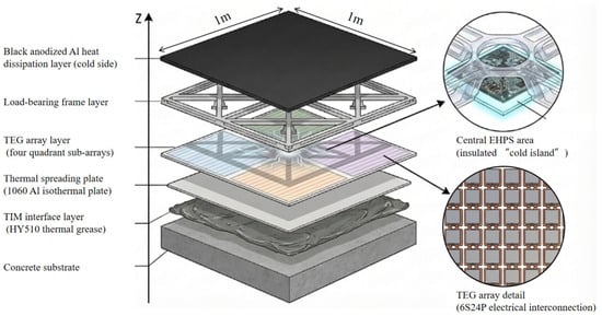
As shown in Figure 1, the physical structure of the Energy Tile comprises a concrete substrate layer, an interfacial gap-filling layer, a heat-flux coupling layer (a thin vapor chamber), a TEG array layer (including four sub-arrays and a central EHPS region), a load-bearing frame layer, and a thin heat-dissipation layer. Within the central EHPS region, a thermal insulation pad (aerogel pad) is introduced to thermally isolate the electronic unit.

Figure 1. Exploded three-dimensional view of the hierarchical physical structure of the 1 m² Energy Tile.

The principal components of the prototype and their physical parameters are summarized in Table 1. The material parameters of the TEG-12706 (purchased from SEEBECK Flagship Store, Guangzhou, China) used in this article are as follows: a Seebeck coefficient of 190–230 μV/K, electrical conductivity of 8.5 × 10⁴–1.25 × 10⁵ S/m, thermal conductivity of 1.2–1.6 W/(m·K), and ZT = 0.9–1.1. TEG-12706 was selected as a commercially available Bi₂Te₃-based module for near-room-temperature harvesting [29]. Rather than targeting single-module extreme low-ΔT performance, the selection emphasized array-level matching, since usable output under low temperature differences depends on Seebeck response, internal resistance, and compatibility with the subsequent power-management circuit [30].

Table 1. Key components and physical parameters of the 1 m² formwork-integrated thermoelectric energy-harvesting prototype.

Component/Layer	Material or Model	Quantity/Configuration	Key Parameters
Interfacial gap-filling layer	HY510 thermally conductive silicone grease	Thin-layer coating applied to the contact interface	Thermal conductivity: 5.0 W/(m·K)
Heat-flux coupling layer	1060 aluminum	1 piece (1 m2)	Thickness: 2 mm
Thermoelectric generator unit	Bismuth telluride TEG-12706	144 units (12 × 12 array), 6 in series and 24 in parallel	Dimensions: 40 × 40 × 3.7 mm; internal resistance: 1.98–2.30 Ω
Load-bearing frame layer	5083-H116 aluminum alloy frame	1 set	Tensile strength: ≥310 MPa
Heat-dissipation layer	5052 black anodized aluminum	1 piece (1 m2)	Thickness: 0.5 mm
EHPS central insulation layer	Nano-aerogel felt	Locally installed in the central EHPS region	Thickness: 3 mm

The effective temperature difference available for thermoelectric energy harvesting is strongly constrained by the interfacial thermal contact resistance at the hot side. Owing to the relatively low thermal conductivity and pronounced surface roughness of concrete [31] (k_con ≈ 1.5 W/(m·K), R_a ≈ 50–100 μm), direct contact with a ceramic substrate readily gives rise to microscale interfacial voids. These voids form an air-dominated low-conductivity layer and introduce a non-negligible temperature drop across the interface.

To quantitatively evaluate the extent of interfacial optimization, this study adopts the areal thermal resistance, R″, as an engineering measure. For a thin gap-filling medium, it may be approximated as

$${\mathrm{R}}^{″}\approx {\displaystyle \frac{\mathrm{t}}{\mathrm{k}}}$$

(1)

where t is the equivalent gap thickness, and k is the thermal conductivity of the gap-filling medium. For the case of direct contact, taking t ≈ Ra = 50–100 μm and k_air ≈ 0.026 W/(m·K), one obtains R_air″ ≈ (1.9–3.8) × 10⁻³ m²·K/W.

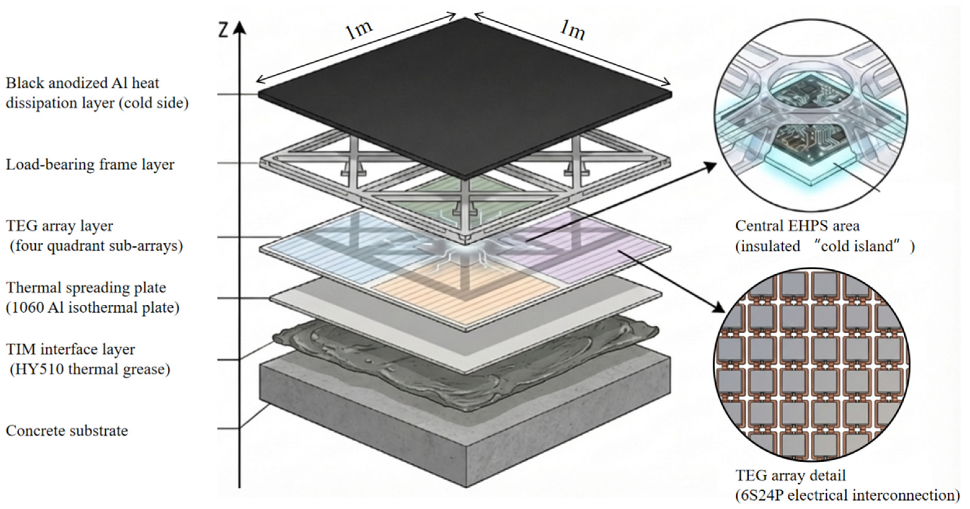
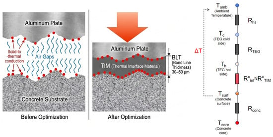
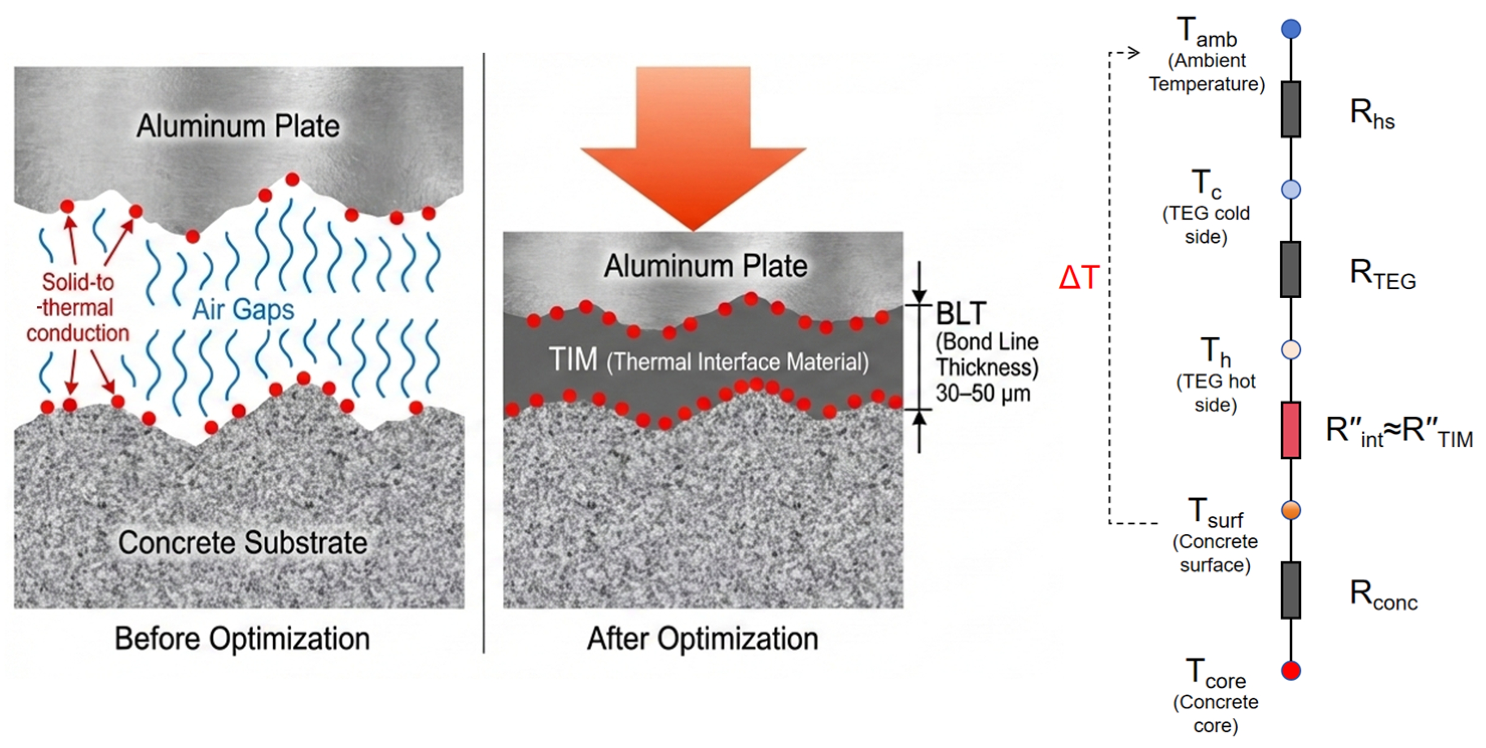
As shown in Figure 2, this study introduces HY510 (purchased from SEERY Flagship Store, Guangzhou, China) thermally conductive silicone grease (k_TIM = 5.0 W/(m·K)) between the concrete and the 1060 aluminum vapor chamber as an interfacial gap-filling layer. Under the lateral pressure applied during construction, the material forms a stable bond-line thickness (BLT ≈ 30–50 μm), yielding R_TIM″ ≈ (0.6–1.0) × 10⁻⁵ m²·K/W. Accordingly, the hot-side interfacial thermal resistance is reduced from R_air″ to R_TIM″, corresponding to a reduction factor of approximately R_air″/R_TIM″ ≈ 2.0 × 10²–6.4 × 10², or about 2.3–2.8 orders of magnitude. In the present system, the thin vapor chamber is used as a passive in-plane heat spreader under the assembled boundary condition, rather than as an independently optimized two-phase component. Since vapor chamber performance is typically assessed by thermal resistance and start-up behavior, both of which depend on structural design and heat input, this study evaluates only the integrated Energy Tile and does not claim a complete characterization of the vapor chamber itself, particularly at low heat flux [32,33].

Figure 2. Optimization mechanism of the concrete–vapor chamber interfacial thermal contact resistance and the corresponding thermal-resistance network model.

2.2. Energy Harvesting and Power Management

Thermoelectric energy harvesting driven by the heat of concrete hydration is characterized by a low initial temperature gradient, a time-decaying power output, and a source impedance that varies with operating conditions. Accordingly, the energy-harvesting circuit must satisfy two engineering requirements simultaneously: first, low-voltage self-start capability under weak temperature-gradient conditions; and second, stable transfer of array output power to a rechargeable energy-storage unit over a wide input range, while preventing instability of the input operating point and repeated system resets caused by the pulsed load of LoRa transmission.

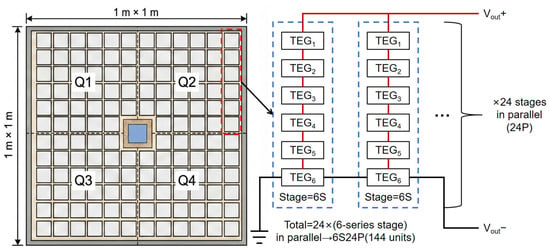
On the harvesting side, the system adopts a combined strategy of topology matching and dual-path harvesting. As shown in Figure 3, the 1 m² prototype incorporates 144 TEG modules (12 × 12), arranged in four quadrant-based partitions with centralized power collection. The array is configured in a 6S24P topology, where the series connection elevates the usable input voltage under weak temperature-gradient conditions, while the parallel connection reduces the equivalent internal resistance and thereby enhances power throughput. To accommodate both ultra-low-temperature-difference cold start and steady-state energy transfer, two harvesting paths are connected in parallel. The cold-start path employs the LTC3108 with a coupled transformer (purchased from Xiangyang Microelectronics, Shenzhen, China), which uses a start-up voltage as low as approximately 20 mV to precharge an intermediate storage capacitor. The primary transfer path uses the LTC3119 (purchased from Liankeji Electronics Co., Ltd., Shenzhen, China) to convey harvested energy over an input range of approximately 0.8–12 V, while achieving quasi-maximum power point extraction through input-voltage-clamped MPPC control.

Figure 3. Physical layout of the 1 m² thermoelectric array and its mapping to the electrical topology.

On the load side, an indirect power supply (store-and-forward) strategy is adopted to decouple the energy source from the load. Specifically, the thermoelectric harvesting chain is responsible only for transferring energy to the storage node, V_store. The microcontroller and continuous loads, including sensing and data storage, are powered through the TPS63070 (purchased from Kangwei Technology, Chengdu, China), which regulates the system voltage to V_sys = 3.3 V. Pulsed events such as LoRa uplink transmission are triggered only when the storage-node voltage satisfies the prescribed condition, and the transient current during transmission is supplied primarily by the storage unit together with a parallel buffer capacitor. This design prevents the collapse of the harvesting-side operating point during pulse events and thereby avoids repeated system resets.

The energy-management strategy defines the system state machine through voltage thresholds and hysteresis, including the RF enable threshold V_TX = 3.75 V, the minimum logging threshold V_LOG = 3.45 V, the undervoltage threshold V_UV = 3.2 V, and a hysteresis band of ΔV_h = 0.15 V. When V_store ≥ V_TX, data transmission is permitted. When V_LOG ≤ V_store < V_TX, the system performs sensing and local data buffering only, while transmission is suspended. When V_store < V_UV, the system enters undervoltage protection and shuts down nonessential peripherals; normal operation resumes only after the voltage recovers above the relevant threshold plus hysteresis. The main hardware components and device models of the self-powered monitoring node are summarized in Table 2.

Table 2. Main hardware components and device models of the self-powered monitoring node.

Component/Module	Model/Specification	Quantity
Microcontroller development board	STM32L431RCT6 (Boring Technology, Suzhou, China)	1
Buck–boost regulator module	TPS63070	1
Ultra-low-voltage cold-start boost converter	LTC3108-1	1
Main power transfer/MPPC module	LTC3119	1
Power monitoring/current–voltage sensor	INA219 (Jiaxinwei Digital Specialty Store, Dongguan, China)	1
Temperature sensor	DS18B20 (Qinhe Intelligent Technology Store, Jiaozuo, China)	2
LoRa communication module	L33_433UD22S (Tashi Flagship Store, Jinhua, China)	1
Energy storage unit	18650 battery (4.8 Wh) (Delipow Flagship Store, Huizhou, China)	1
Local storage	MB85RC256V (Mingwu Electronics, Shenzhen, China)	1

In the present study, the 18650 battery is adopted only as the storage unit required for prototype-level experimental validation. In future engineering applications, multiple 1 m² Energy Tile units may be connected to a shared battery installed in a fixed electrical box, rather than using one distributed battery for each unit.

2.3. Sampling Strategy and Energy Consumption Model

To balance the continuity of maturity-related temperature monitoring against the constraints imposed by limited harvested energy, the node adopts a high-frequency sampling, low-frequency transmission strategy. Specifically, temperature data are acquired at a fixed sampling interval, T_s, and written to local cache memory; at a transmission interval, T_u, N = T_u/T_s records are aggregated and uploaded in a single LoRa uplink packet. During undervoltage-induced transmission suspension, data acquisition and local buffering continue uninterrupted, and the buffered records are retransmitted in batches once the voltage recovers. In this way, insufficient energy manifests as transmission delay rather than monitoring failure.

The node energy consumption is represented using an event-driven model. Over an evaluation horizon T, the total energy consumption is given by

$${\mathrm{E}}_{\mathrm{o}\mathrm{u}\mathrm{t}}(\mathrm{T})\approx ({\mathrm{P}}_{\mathrm{s}\mathrm{l}\mathrm{e}\mathrm{e}\mathrm{p}}+{\mathrm{P}}_{\mathrm{q}})\mathrm{T}+[{\displaystyle \frac{\mathrm{T}}{{\mathrm{T}}_{\mathrm{s}}}}]{\mathrm{E}}_{\mathrm{s}}+[{\displaystyle \frac{\mathrm{T}}{{\mathrm{T}}_{\mathrm{u}}}}]{\mathrm{E}}_{\mathrm{u}}+{\mathrm{N}}_{\mathrm{t}\mathrm{r}}{\mathrm{E}}_{\mathrm{t}\mathrm{r}}$$

(2)

where E_s denotes the energy consumed per sampling event (including sensing, computation, and data writing); E_u denotes the energy consumed per transmission event (including wake-up, packet formation, and RF transceiving); P_sleep denotes the average power consumption of the node in sleep mode; P_q denotes the aggregate quiescent background power of the always-on or standby load-side circuits; E_tr denotes the lumped energy overhead per state-transition event, including threshold switching, entry/exit of undervoltage protection; and N_tr denotes the total number of such state-transition events within the evaluation horizon. The typical ranges and the values adopted for the energy-consumption model parameters of the self-powered monitoring node are summarized in Table 3.

Table 3. Energy consumption model parameters of the self-powered monitoring node: typical ranges and values adopted in this study.

Symbol	Parameter	Unit	Value
Ts	Sampling interval	min	30
Tu	Transmission interval	h	4
N	Number of records per transmission	–	8
Vsys	System supply voltage	V	3.3
Psleep	Average sleep-mode power consumption	W	1–10 × 10−5
Pq	Standby static power consumption	mW	0.28–0.68
Es	Energy consumed per sampling event	mJ	30–100
Eu	Energy consumed per transmission event	J	1–5
Etr	Single-switching energy consumption	µJ	5–100
Ntr	Number of state-transition events	–	84
SF	Spreading factor	–	12
BW	Bandwidth	kHz	125
TxPower	Transmission power	dBm	22
Payload	Payload length	bytes	40

Note: The typical parameter ranges reported in Table 3 are drawn from device datasheets and commonly adopted configurations in the relevant literature. The upper-bound values of these parameters are used in the present calculations.

2.4. Calibration of the Standard Sub-Array

To convert the simulated temperature difference series, ΔT(t), obtained in the subsequent numerical analysis of the system-level usable electrical power input, this study conducts laboratory calibration using a standard sub-array that is structurally homologous to the 1 m² prototype. The objective is to establish the mappings of V–ΔT and P–ΔT under realistic interfacial treatment and wiring conditions, and to extract derating factors for system-level estimation. The standard sub-array corresponds to one physical quadrant of the 1 m² prototype and consists of 36 TEG units arranged in a 6 × 6 matrix and integrated onto a 250 mm × 250 mm aluminum-alloy vapor chamber. The interfacial materials are identical to those used in the full-scale prototype, including the thermally conductive gap-filling medium and vapor-chamber coupling layer. Stable contact conditions are ensured by a clamping fixture so as to reproduce the assembly boundary conditions of the experiment. The electrical configuration of the sub-array is fixed at 6S6P, thereby preserving structural homology with respect to the number of series-connected units in the full 1 m² system (6S24P). Under this configuration, the open-circuit voltage of the sub-array is of the same order of magnitude as that of the full system, while the short-circuit current scales with the quadrant size, allowing the measured voltage–temperature difference relationship to be used directly for evaluating the startup and sustained-operating feasibility of the main power-management path.

The experimental program combines two complementary tests: steady-state temperature-difference scanning and continuous duration-based validation. The first is a steady-state temperature-difference scanning calibration test, designed to establish the quantitative relationship among temperature difference, voltage, and power for the sub-array. Over the range of ΔT = 5–50 °C, with the cold-side temperature T_c maintained at 0 °C and the hot-side temperature T_h varied from 5 °C to 50 °C, target temperature differences are applied incrementally at intervals of 5 °C. At each target point, the real-time temperatures of the hot and cold sides are synchronously recorded, and data acquisition proceeds only after the system satisfies the steady-state criterion, defined as ∣dΔT/dt∣ < 0.1 °C sustained for 3 min. The key calibration outputs are the input operating-point voltage after matching with the energy-management circuit, V_in,PMIC, and the corresponding input power, P_in,PMIC.

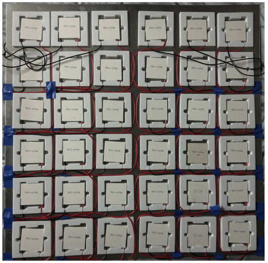
The second test is a continuous measurement designed to represent the time-varying temperature difference at the concrete surface, and is intended to verify the output consistency and operational reliability of the sub-array under diurnal temperature fluctuations simulating concrete hydration heat. The hot-side temperature is controlled by a programmable heat source to emulate the concrete surface temperature, T_surf (20–30 °C), while the cold-side temperature is taken as the laboratory ambient temperature, T_amb. Under the same contact conditions, the temperatures at the hot and cold sides, together with the output voltage and current of the sub-array, are continuously recorded. The sampling interval is set at 30 min, and the total test duration is 3 d, covering 144 sampling points. A photograph of the experimental platform for the standard sub-array is shown in Figure 4.

Figure 4. Photograph of the experimental platform for the standard sub-array.

2.5. Temperature-Difference Simulation and System-Level Energy Evaluation

To evaluate the practical availability of thermoelectric energy harvesting during the curing period, this study employed a transient temperature-field simulation using an in-house program developed by the authors’ research group to obtain the time history of the surface temperature over the Energy Tile coverage area, Tsurf(t). This series is then combined with the ambient air temperature input, T_amb(t), to construct the driving temperature-difference sequence, ΔT(t) = T_surf(t) − T_amb(t).

2.5.1. Temperature-Field Model and Boundary Conditions

At any point within the concrete computational domain R, the transient temperature field, T(x, y, z, t), must satisfy the governing heat-conduction equation:

$${\displaystyle \frac{\partial \mathrm{T}}{\partial \mathrm{t}}}=\alpha ({\displaystyle \frac{{\partial }^2\mathrm{T}}{{\partial \mathrm{x}}^2}}+{\displaystyle \frac{{\partial }^2\mathrm{T}}{{\partial \mathrm{y}}^2}}+{\displaystyle \frac{{\partial }^2\mathrm{T}}{{\partial \mathrm{z}}^2}})+{\displaystyle \frac{\partial \theta }{\partial \tau }}(\forall (\mathrm{x},\mathrm{y},\mathrm{z})\in \mathrm{R})$$

(3)

where T—temperature (°C); α—thermal diffusivity (m²/h); θ—adiabatic temperature rise in concrete (°C); t—time (d); and τ—age (d).

The boundary conditions are specified in accordance with standard forms commonly used in engineering thermal analysis, including prescribed-temperature boundaries, adiabatic boundaries, and surface heat-exchange boundaries. Because the present study focuses on energy harvesting driven by the surface-to-ambient temperature difference, the critical boundary condition is the heat-exchange condition at the external surface, which is represented by a third-kind boundary condition:

$$\lambda {\displaystyle \frac{\partial \mathrm{T}(\mathrm{x},\mathrm{y},\mathrm{z},\mathrm{t})}{\partial \mathrm{n}}}=\beta (\mathrm{T}(\mathrm{x},\mathrm{y},\mathrm{z},\mathrm{t}))-{\mathrm{T}}_{\mathrm{a}}(\mathrm{x},\mathrm{y},\mathrm{z},\mathrm{t})$$

(4)

where β—heat transfer coefficient (kJ/(m²·h·°C)); λ—thermal conductivity of the material (kJ/(m·h·°C)); and Ta—ambient temperature (°C).

For the calculations, the variation in the multi-year average daily air temperature for Liaoning Province, China, was fitted using the following equation:

$${\mathrm{T}}_{\mathrm{a}}(\mathrm{t})=8+16.65\times \cos [{\displaystyle \frac{\pi }{6}}(\mathrm{t}-7)]$$

(5)

The diurnal temperature-difference function is given by

$${{\mathrm{T}}_{\mathrm{a}}}^{\mathrm{d}}(\tau )={\mathrm{T}}_{\mathrm{a}}(\mathrm{t})+5\times \cos [{\displaystyle \frac{\pi }{12}}(\tau -12)]$$

(6)

2.5.2. Model Geometry and Mesh

The geometric model was developed from the actual structural configuration of a gravity dam in Liaoning Province, China, with appropriate geometric simplifications applied. The simulation domain includes the core region of the dam body, the external surfaces, and the portions exposed to the surrounding environment. The material properties used in the model are summarized in Table 4.

Table 4. Thermophysical properties adopted for numerical simulation of the concrete temperature field.

Concrete Grade	Thermal Conductivity, λ (kJ/(m·h·°C))	Specific Heat, c (kJ/(kg·°C))	Thermal Diffusivity, a (m2/h)	Linear Expansion Coefficient, α (10−6/°C)	Ultimate Adiabatic Temperature Rise, θ0 (°C)
C20	12.09	1.0076	0.00502	7.54	28.5

As shown in Figure 5, the geometric model was discretized using a free hexahedral mesh in HyperMesh 2019 (Altair Engineering Inc., Troy, MI, USA). The model comprises 10,738 elements and 13,468 nodes, and a mesh-independence analysis was subsequently performed.

Figure 5. Schematic of the geometric model for numerical temperature-field simulation and the locations of monitoring points.

2.5.3. Simulation Scenarios and Temperature-Difference Output

To account for the influence of seasonal variation on the energy-harvesting window, four representative ambient-temperature scenarios—spring, summer, autumn, and winter—were constructed in this study. For each scenario, a continuous evaluation window of T = 7 d was adopted. The representative weekly periods for spring, summer, autumn, and winter were defined as 15–22 April, 15–22 July, 15–22 October, and 15–22 January, respectively. The casting temperature was taken as the long-term average daily mean air temperature plus 3 °C, with no additional temperature-control measures applied. Because the Energy Tile is composed primarily of aluminum plates with high thermal conductivity, and because the interfacial thermal resistance of the bonding layer (thermally conductive silicone grease) is very small, the equivalent heat-transfer capacity of the Energy Tile-covered region is comparable to that of conventional steel formwork when expressed in terms of the third-kind boundary heat-transfer coefficient. In this study, β_d = 400 kJ/(m²·d·°C) was adopted. The output time step of the temperature-field simulation, ΔT(t), was set to 3 h, consistent with the subsequent energy-integration interval, so that ΔT(t) could be directly mapped into a power time series for cumulative energy estimation.

2.5.4. System-Level Energy Estimation and ENO/ESF Criteria

Based on the experimentally calibrated temperature-difference-to-power relationship obtained for the standard sub-array in Section 2.4, together with the hourly temperature-difference series generated by the numerical simulation in Section 2.5.3, the system-level energy yield of the 1 m² prototype over the full curing period was quantified. The feasibility of self-powered operation under different working conditions was then evaluated using the criteria of energy-neutral operation (ENO) and the energy safety factor (ESF).

(1)

Calculation of system-level thermoelectric output power

The real-time thermoelectric output power of the 1 m² prototype system is calculated as follows:

$${\mathrm{P}}_{\mathrm{T}\mathrm{E}\mathrm{G}}\left(\mathrm{t}\right)={\mathrm{N}}_{\mathrm{q}}·{\mathrm{P}}_{\mathrm{s}\mathrm{u}\mathrm{b}}(\Delta \mathrm{T}(\mathrm{t}\left)\right)$$

(7)

where N_q = 4 is the quadrant scaling factor, since the standard sub-array corresponds to one-quarter of the physical 1 m² prototype. P_sub(ΔT(t)) denotes the experimentally measured effective output power (W) of the standard sub-array under the instantaneous temperature difference ΔT(t), as obtained from the calibration in Section 2.4. The boundary condition is specified as follows: when ΔT(t) ≤ 0, the thermoelectric modules produce no effective output, and thus P_TEG(t) = 0.

After conversion by the power management unit (PMU), the real-time effective power delivered from the thermoelectric harvesting system to the energy-storage unit is given by

$${\mathrm{P}}_{\mathrm{i}\mathrm{n}}\left(\mathrm{t}\right)={\eta }_{\mathrm{p}\mathrm{m}\mathrm{u}}·{\mathrm{P}}_{\mathrm{T}\mathrm{E}\mathrm{G}}\left(\mathrm{t}\right)$$

(8)

where η_PMU is the experimentally measured average conversion efficiency of the power management circuit. This value is obtained from the steady-state tests of the circuit described in Section 2.2 over its typical operating range. In this study, the measured mean value of 85% is adopted to represent the conversion performance across the full range of operating conditions, from weak to strong temperature differences.

(2)

Trapezoidal integration for cumulative input energy

To account for the nonlinear temporal decay of the temperature difference induced by concrete hydration heat, the trapezoidal integration method is employed. Over the evaluation window of T = 7, the cumulative input energy is obtained by integrating P_in(t) as follows:

$${\mathrm{E}}_{\mathrm{i}\mathrm{n}}(7\mathrm{d})={\sum }_{\mathrm{K}=1}^{\mathrm{K}-1}{\displaystyle \frac{{\mathrm{P}}_{\mathrm{i}\mathrm{n}}\left({\mathrm{t}}_{\mathrm{k}}\right)+{\mathrm{P}}_{\mathrm{i}\mathrm{n}}\left({\mathrm{t}}_{\mathrm{k}+1}\right)}{2}}·∆\mathrm{t}$$

(9)

where K is the total number of sampling points within the evaluation window. For a 7-day evaluation period with a time step of 3 h, K = 57; Δt is the time interval (h) between two adjacent sampling points, which is fully consistent with the output time step of the numerical temperature-field simulation, and is taken here as Δt = 3; and t_k denotes the time corresponding to the k-th sampling point.

The monitoring-side energy demand, E_out(7 d), is calculated using the energy-consumption model presented in Section 2.3, covering the full operating-cycle demand associated with node sleep, periodic sensing, local data storage, and wireless data transmission.

(3)

Quantitative evaluation framework based on the ENO criterion and ESF

During the evaluation period, if the cumulative effective input energy of the system is greater than or equal to the total energy consumption requirement of the monitoring system under all operating conditions, it is determined that the system can achieve fully autonomous energy-neutral operation. The criterion expression is E_in(7 d) ≥ E_out(7 d). The establishment of ENO indicates that under this operating condition, the system can maintain the continuous and stable operation of the monitoring node solely by the energy collected from hydration heat thermoelectricity, without the need for an external power supply or pre-charging of energy storage units for supplementation.

To quantify the energy margin, the energy safety factor (ESF) is defined as

$$\mathrm{E}\mathrm{S}\mathrm{F}={\displaystyle \frac{{\mathrm{E}}_{\mathrm{i}\mathrm{n}}\left(7\mathrm{d}\right)}{{\mathrm{E}}_{\mathrm{o}\mathrm{u}\mathrm{t}}\left(7\mathrm{d}\right)}}$$

(10)

An ESF greater than 1 indicates an energy surplus, and a larger ESF corresponds to a greater energy margin.

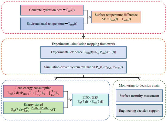
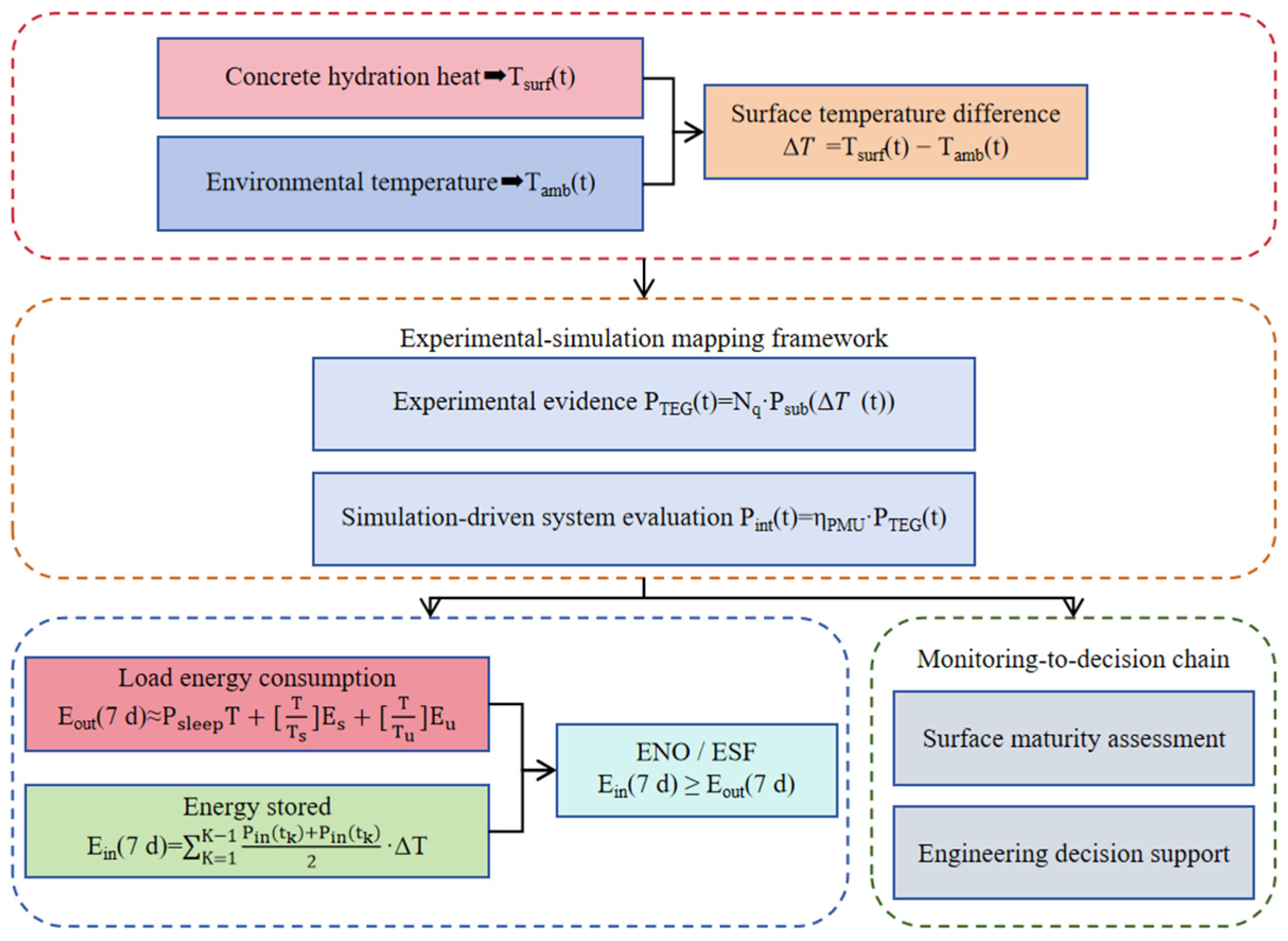
Based on the above temperature-difference inputs, experimentally calibrated mapping relationships, and energy-calculation procedures, this study establishes a system-level evaluation framework for self-powered operation (see Figure 6). The framework integrates the surface-to-ambient temperature-difference input, thermoelectric output mapping, power-management correction, and node load demand into a unified analytical workflow, thereby providing the basis for energy-yield calculation and ENO/ESF evaluation. In the present study, the monitoring system mainly records surface temperature histories. These logged data may serve as a possible downstream input for project-specific maturity/strength interpretation and support for formwork-removal timing after proper calibration, but such engineering interpretation is not evaluated here. A direct thermal-cracking risk assessment is beyond the scope of the present study and would require additional internal-temperature information and/or temperature-field or thermo-mechanical analysis.

Figure 6. Schematic illustration of the evidence chain for the self-powered monitoring system.

3. Results

3.1. Sub-Array Calibration Results

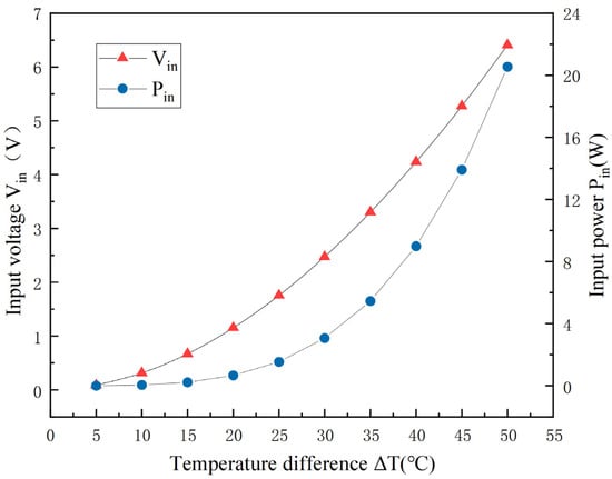
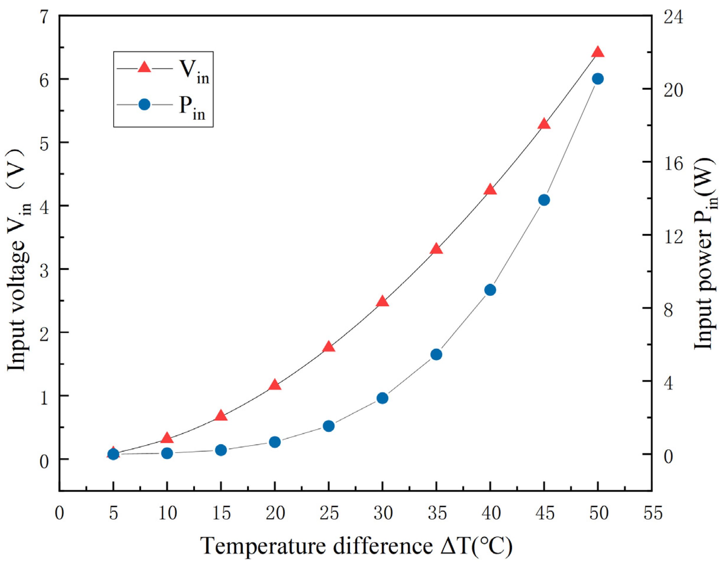
Figure 7 presents the relationships between the input operating-point voltage, Vin, and the corresponding input power, Pin, of the energy-harvesting path and the applied temperature difference for the standard sub-array (36 units, 6S6P) under steady-state temperature-difference scanning (ΔT = 5–50 °C, in increments of 5 °C). As ΔT increases, Vin rises monotonically from 0.088 V at 5 °C to 6.411 V at 50 °C, while the corresponding Pin increases from 0.004 W to 20.55 W. These results indicate that the energy margin is extremely limited in the low-temperature-difference regime: when ΔT ≤ 10 °C, Pin ≤ 0.049 W; by contrast, once ΔT ≥ 20 °C, the input power increases markedly with temperature difference, reaching 0.665 W at 20 °C and 8.982 W at 40 °C. This pattern suggests that the system is constrained by limited available input power during the weak-temperature-difference startup stage, whereas it acquires a more stable energy-transfer capability once it enters the moderate temperature-difference range.

Figure 7. Relationship of the PMIC input operating-point voltage and input power of the standard sub-array with temperature difference under steady-state temperature-difference scanning.

3.2. Output Consistency in Testing

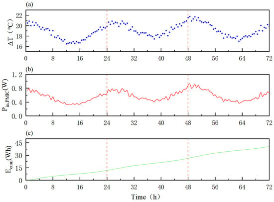
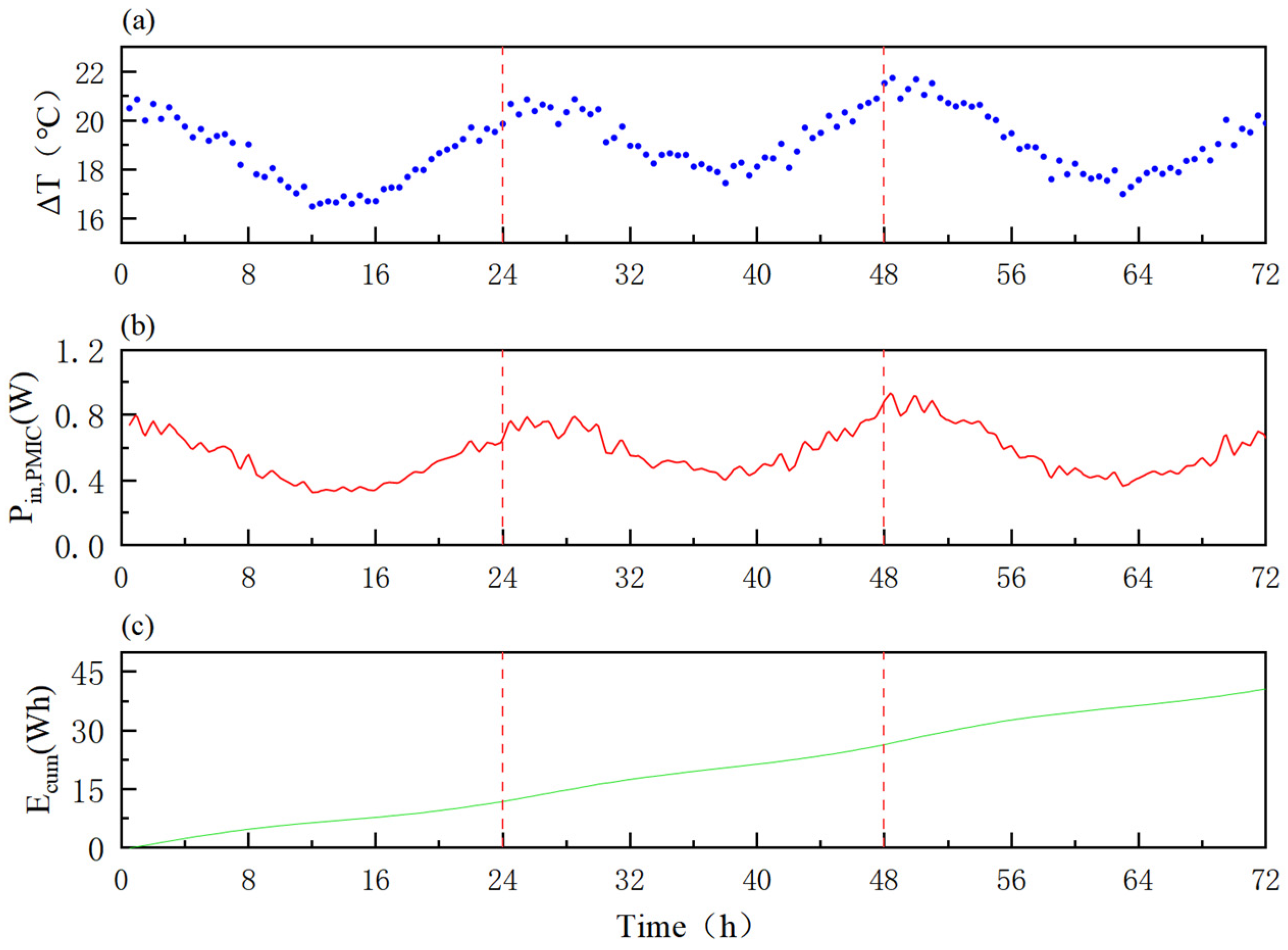
Figure 8a shows that the temperature difference, ΔT(t) = Thot(t) − Tcold(t), exhibited a stable diurnal fluctuation over 72 h, ranging from 16.45 to 21.7 °C. The corresponding PMIC input power, Pin, PMIC(t), shown in Figure 8b, varied synchronously with ΔT(t), with a fluctuation range of approximately 0.33–0.92 W. No obvious time-accumulated drift or abrupt change was observed. The cumulative input energy, Ecum, obtained by trapezoidal integration, is presented in Figure 8c, reaching 40.68 Wh at the end of the 72 h period, which corresponds to an average input power of approximately 0.565 W over the three-day test.

Figure 8. Validation of the output consistency of the standard sub-array under continuous temperature-difference fluctuations over 72 h: (a) time history of the temperature difference; (b) time history of the input power; and (c) time history of the cumulative input energy.

3.3. Seasonal Temperature-Difference Simulation

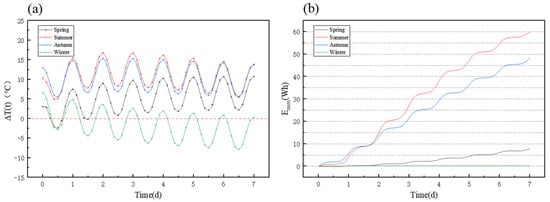
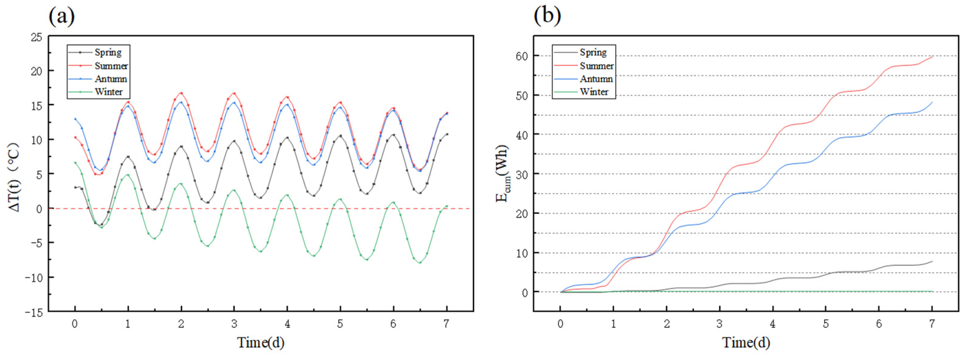
Figure 9 illustrates the evolution of the concrete surface-to-ambient temperature difference, ΔT(t), and the cumulative input energy, Ecum(t), over representative weeks in the four seasons. The simulation time step was 3 h, yielding a total of 57 sampling points over each 7-day period. Substantial seasonal differences are observed in both the magnitude and persistence of the temperature difference, and these differences are directly reflected in the cumulative energy-growth profiles. In spring, ΔT fluctuates between −2.3 °C and 10.8 °C, with an average of 4.9 °C. During limited periods, ΔT < 0, indicating that the surface temperature falls below the ambient temperature; by the end of the 7-day period, Ecum(t) reaches 7.87 Wh. In both summer and autumn, the temperature difference remains positive and at a comparatively high level throughout the representative week. Specifically, ΔT ranges from 5.0 °C to 16.8 °C in summer, with an average of 11.0 °C, and from 5.5 °C to 15.4 °C in autumn, with an average of 10.4 °C. The corresponding cumulative energies over 7 d reach 59.79 Wh and 48.28 Wh, respectively. In winter, by contrast, the temperature difference is generally small. Over the representative week, the effective temperature difference—defined on the harvesting side as ΔT > 0 only—has a maximum of approximately 6.7 °C and an average of 0.8 °C, while the duration of positive temperature difference is substantially shorter than in the other seasons. As a result, the cumulative energy increases only slowly, reaching 0.234 Wh. Overall, the cumulative input energy follows the order summer > autumn > spring ≫ winter.

Figure 9. Simulated time-history curves over representative weeks (7 d) in the four seasons: (a) concrete surface-to-ambient temperature difference, ΔT(t); (b) cumulative input energy, Ecum(t).

3.4. System Energy and ENO/ESF

The numerical simulation results reveal pronounced seasonal differences in the cumulative input energy of the system. Driven by persistently high positive temperature differences, the cumulative input energy over 7 d reaches 59.79 Wh in summer and 48.28 Wh in autumn. In spring, owing to fluctuations in the temperature difference, the 7-day cumulative input energy decreases to 7.87 Wh. In winter, by contrast, the cumulative input energy is limited to only 0.23 Wh because of the small temperature difference and the short effective harvesting window.

To ensure a conservative evaluation, this study adopts the highest-power-consumption operating condition as a uniform benchmark and calculates energy demand using the upper-bound values of the relevant parameters. Over the 7-day evaluation window, this corresponds to 336 sampling events and 42 transmission events, yielding E_out(7 d) = 0.1987 Wh. Under the representative spring, summer, autumn, and winter scenarios, the cumulative effective input energy of the system over 7 d satisfies the ENO criterion in all cases (E_in(7 d) ≥ E_out(7 d)), indicating that fully self-sustained operation can be achieved solely through energy recovered from hydration heat. The core evaluation results for self-powered operation under the four seasonal scenarios are summarized in Table 5.

Table 5. Evaluation results of self-powered operation under representative seasonal scenarios.

Season	Ein(7 d) (Wh)	Eout(7 d) (Wh)	ESF	ENO
Spring	7.87	0.1987 (highest-power-consumption scenario)	39.61	Satisfied
Summer	59.79		300.89	Satisfied
Autumn	48.28		242.97	Satisfied
Winter	0.23		1.16	Satisfied

All four seasonal scenarios yield ESF values greater than 1 under the revised conservative load model. Energy surpluses remain substantial in summer, autumn, and spring, whereas the winter scenario satisfies the ENO criterion with only a limited energy margin. Under winter conditions, operational feasibility is therefore more sensitive to interfacial thermal resistance, background quiescent consumption, the state of energy storage, state-transition overhead, and load-scheduling strategies.

4. Discussion

4.1. Core Mechanism Analysis

4.1.1. Hydration Heat Utilization

In this study, the heat released during cement hydration is treated as a transient, decaying heat source [34]. The thermoelectric conversion process is driven by the surface-to-ambient temperature difference, ΔT(t), that develops during the early-age stage, thereby enabling recovery of energy that would otherwise be dissipated as wasted hydration heat. The central mechanism lies in the alignment between hydration-heat release and monitoring demand across both temporal and spatial scales.

From a temporal perspective, hydration heat is highly concentrated during the early period after casting, and the concrete surface temperature, T_surf(t), follows a nonstationary evolution characterized by temperature rise–peak–decay. This pattern coincides closely with the period of rapid temperature-field variation and heightened susceptibility to thermal cracking [4]. By taking ΔT(t) = T_surf(t) − T_amb(t) as the driving variable, the time-varying nature of the heat source is translated into usable power input, thereby establishing a temporal coupling between heat-source decay and adaptive load response.

From a spatial perspective, hydration heat accumulates within the structure and is conducted toward the formwork side, where it combines with surface convective heat exchange to form a stable heat-flow pathway. By integrating thermoelectric modules on the formwork side, the system couples with this heat flux and directly converts the temperature difference without intruding into the structural interior. At the same time, the introduction of a controllable heat-dissipation path on the formwork side gives the system potential engineering value not only for energy recovery but also for regulating thermal behavior [35].

4.1.2. Interfacial Resistance Optimization

Thermoelectric output is constrained by the effective temperature difference across the hot and cold sides of the module, ΔT_TEG, while the concrete–thermoelectric module interfacial contact resistance, R_int″, often governs how the temperature drop is distributed along the heat-transfer path and therefore constitutes the principal source of attenuation in ΔT_TEG. Let the areal thermal resistance, R″, denote the heat-transfer resistance of each layer. Under unoptimized direct contact, R_int,air″ ≈ t/k_air = (1.9–3.8) × 10⁻³ m²·K/W in room-temperature conditions. This places R_int,air″ on the same order of magnitude as R_TEG″ (3.7 × 10⁻³ m²·K/W) and R_conc″ (3.3 × 10⁻³ m²·K/W). After introducing HY510 thermally conductive silicone grease as the gap-filling layer, a stable bond-line thickness of 30–50 μm is formed under lateral pressure during construction. With k_TIM = 5.0 W/(m·K), the resulting interfacial resistance is estimated as R_int,TIM″ ≈ (0.6–1.0) × 10⁻⁵ m²·K/W, representing a reduction of approximately two to three orders of magnitude relative to the air-gap case. This substantially preserves the temperature difference available for thermoelectric conversion, ΔT_TEG.

4.2. Seasonal Thermal Behavior and Harvesting

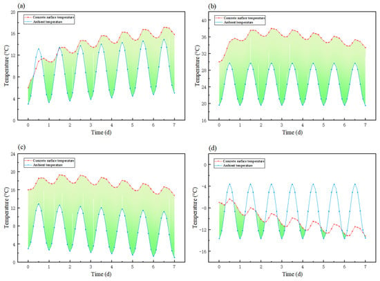
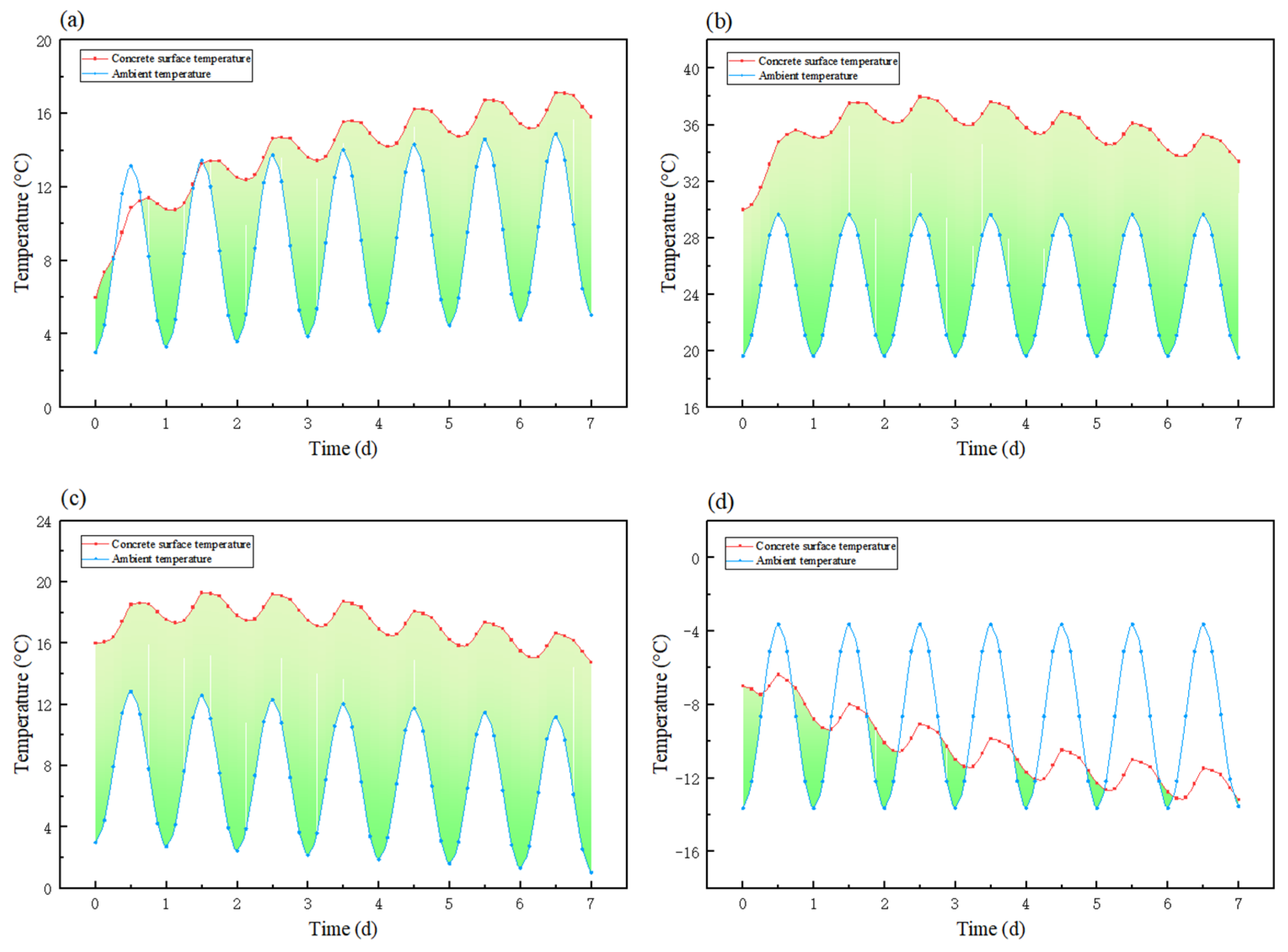
Figure 10 compares the temperature histories under the four seasonal scenarios. Overall, T_surf(t) rises rapidly during the initial post-casting period and then gradually enters a slowly varying stage, whereas T_amb(t) is dominated by diurnal fluctuations. Their interaction causes ΔT(t) to exhibit a combined pattern of nonstationarity associated with early-age evolution and periodicity associated with daily oscillation, thereby determining seasonal differences in the effective harvesting window and the available energy margin.

Figure 10. Time-history profiles of concrete surface temperature and ambient temperature over representative weeks in the four seasons: (a) spring; (b) summer; (c) autumn; (d) winter.

4.2.1. Seasonal Differences in Thermal Behavior

Across all seasonal scenarios, the concrete surface temperature exhibits a cyclical pattern jointly governed by the initial casting temperature and the release of hydration heat during the early-age stage; however, its relationship with ambient temperature is strongly shaped by seasonal boundary conditions. As shown in Figure 10, the surface temperature remains generally higher than the ambient temperature in spring, summer, and autumn. In summer and autumn, in particular, a sustained and stable positive temperature difference is maintained, corresponding respectively to continuously high and moderately stable thermal driving conditions. In spring, although the temperature difference remains positive overall, it is more strongly affected by diurnal fluctuations, with brief intervals of negative temperature difference occurring locally; the availability of the temperature gradient is therefore more variable. By contrast, under winter conditions, despite the elevation of surface temperature by hydration heat, the combined effects of low ambient temperature and intensified heat dissipation lead to frequent alternation between positive and negative surface-to-ambient temperature differences, yielding an overall weaker thermal-gradient background. This indicates that, in winter, harvesting performance is more sensitive to variations in external boundary conditions. It should be noted that the winter scenario is considered here primarily for comparative analysis under unfavorable conditions. Given that winter is not a principal construction season in northeastern China and similar regions, the significance of the winter results lies mainly in characterizing the lower bound of system performance and providing a reference for assessing applicability under different seasonal conditions. Taken together, these results suggest that seasonal differences do not alter the fundamental evolution of concrete surface temperature at early age, but they substantially affect the duration and stability of the positive surface-to-ambient temperature-difference window, which in turn is the primary determinant of differences in cumulative system input energy.

4.2.2. Temperature-Difference Availability Metrics

Given that thermoelectric output is meaningful only when ΔT(t) > 0, this study uses the duration of positive temperature difference to characterize the continuity of the energy-harvesting window. Based on 3 h intervals over a 7-day period (168 h), the positive-temperature-difference windows are summarized as follows:

(1)

Spring: The positive-temperature-difference duration is approximately 156 h, while the negative-temperature-difference duration is about 12 h. Although the mean temperature difference remains positive (approximately 5.0 °C), brief negative excursions do occur, indicating that spring corresponds to an operating condition that is usable but fluctuating.

(2)

Summer: The positive-temperature-difference duration reaches 168 h, i.e., positive throughout the entire period, with the highest mean ΔT (approximately 11.02 °C). This represents the most favorable operating condition, characterized by high magnitude and strong continuity.

(3)

Autumn: The positive-temperature-difference duration is likewise 168 h, remaining positive throughout, with a mean ΔT of approximately 10.39 °C. This corresponds to a stable operating condition featuring moderately high magnitude and strong continuity.

(4)

Winter: The positive-temperature-difference duration is only about 63 h, whereas the negative-temperature-difference duration reaches approximately 105 h, and the mean ΔT is negative (approximately −1.61 °C). This indicates that the winter harvesting window is highly fragmented, and that system availability depends more critically on interfacial thermal-resistance optimization and adaptive load-energy scheduling.

These results suggest that seasonal differences are reflected not only in ΔT_max but, more importantly, in the cumulative duration of positive temperature difference and the stability of the thermal background. Summer and autumn benefit from long harvesting windows, spring exhibits brief losses of thermal driving, and winter constitutes the most unfavorable boundary condition, characterized by a short window and frequent reversals. The statistical results of the surface-to-ambient temperature-difference characteristics under the representative seasonal scenarios are summarized in Table 6.

Table 6. Statistical results for the surface-to-ambient temperature-difference characteristics under representative seasonal scenarios.

Season	ΔTmin (°C)	ΔTmax (°C)	Average ΔT (°C)	Duration of ΔT > 0 (h)
Spring	−2.26	10.78	5	156
Summer	5.02	16.75	11.02	168
Autumn	5.46	15.37	10.39	168
Winter	−7.83	6.65	−1.61	63

4.3. Consistency and Scale-Up Reliability

4.3.1. Validation of Experimental–Simulation Consistency

(1)

Quantitative mapping relationship

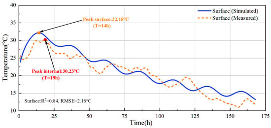
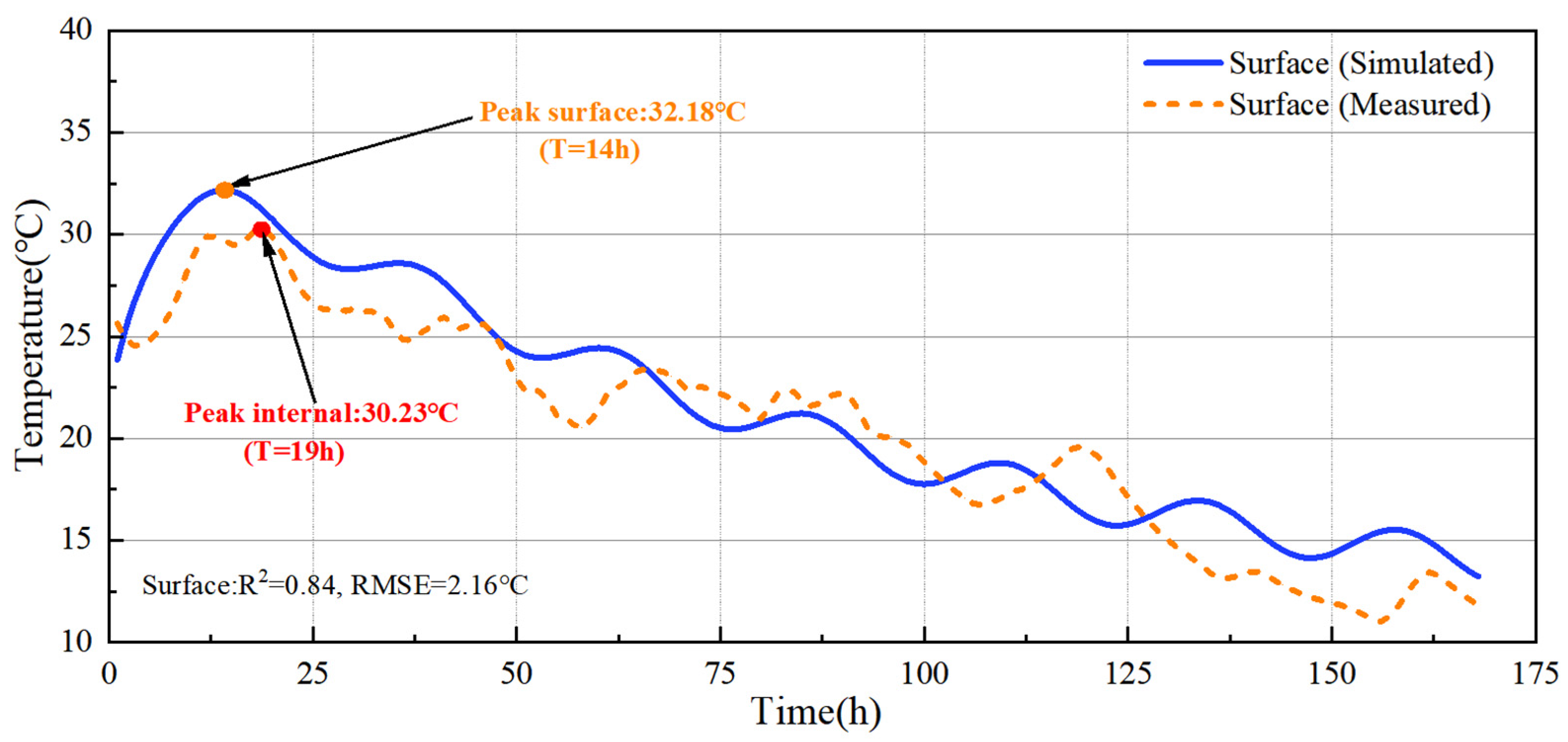
The simulation yields the surface temperature-difference series ΔT = {0, 5, …, 50} °C for the subarray, where V_oc,sub, R_int,sub, V_in,PMIC, and P_in,PMIC are obtained, thereby establishing P_in,PMIC = f(ΔT). During coupling, ΔT(t_k) is mapped to P_in,PMIC(t_k) using piecewise linear interpolation with a step size of 3 h (0.125 d), and a physical constraint of ΔT ≤ 0 ⇒ P = 0 is applied. The mapping mainly occurs within the calibration coverage area, ensuring the robustness of the numerical coupling. To provide a preliminary check on the realism of the simulated thermal evolution, the simulated surface temperature was compared with measured surface-temperature data from a comparable mass-concrete project over the first 168 h after casting (Figure 11). The two curves show consistent heating–cooling evolution, with the simulated peak temperature of 32.18 °C occurring at 14 h and the measured peak temperature of 30.23 °C occurring at 19 h.

Figure 11. Simulated vs. measured surface temperature over 168 h.

(2)

Fidelity of the simulation boundary conditions

The numerical simulation of the concrete temperature field was conducted using the transient heat-conduction equation commonly adopted in engineering practice. The model was developed on the basis of the actual geometry and material properties of a gravity dam in a reservoir in Liaoning Province, China, and the boundary conditions were specified using the conventional third-kind heat-transfer boundary widely employed in engineering thermal analysis. The equivalent heat-transfer coefficient assigned to the Energy Tile-covered region was taken to be consistent with that of steel formwork commonly used in practice. As a result, the thermal boundary conditions closely reflect real construction conditions, and the resulting temperature-difference series follows the physical evolution of the early-age temperature field in mass concrete rather than an idealized laboratory scenario, thereby reducing the risk of overestimating the available temperature gradient under overly simplified experimental boundaries.

4.3.2. Transferability of Scale-Up

The energy-harvesting capability of the 1 m² prototype was estimated from the 0.25 m² standard sub-array on the basis of structural homology and electrical-topology consistency, while deviations from the ideal linear scaling relationship caused by in-plane temperature nonuniformity, branch-to-branch performance dispersion, and contact-resistance variations were further evaluated using a conservative aggregate derating analysis. Under these conditions, the voltage characteristics of the system are governed primarily by the number of series-connected modules, whereas the power output can be expected to scale approximately linearly with the number of parallel branches and the effective area. This scaling approach is therefore most appropriate for formwork-integrated applications in which the temperature-difference field is relatively uniform and array-level fabrication consistency is well controlled.

(1)

Voltage Scale

For both the sub-array and the full-scale system, the number of series-connected modules is the same, namely 6 (6S). Accordingly, under the same driving temperature difference, ΔT, the open-circuit voltage of the array—or, equivalently, the order of magnitude of its effective input voltage—does not change with area scaling, such that V_{oc,1 m}² (ΔT) ≈ V_oc,sub (ΔT). In other words, the 1 m² system and the 0.25 m² sub-array operate within the same voltage regime: the cold-start threshold, the PMIC input-voltage range, and the triggering conditions of the threshold-based state machine all remain unchanged. The voltage-to-temperature-difference calibration obtained from the sub-array can therefore be directly carried over as the voltage-scale basis for the full system.

(2)

Power scale

Provided that the temperature-difference distribution is approximately uniform and the electrical performance of each parallel branch is consistent, the equivalent internal resistance of the parallel network scales inversely with the number of parallel branches. Because the full system uses 24 parallel branches, which is four times the 6P configuration of the sub-array, it follows that R_{int,1 m}² (ΔT) ≈ R_int,sub(ΔT)/4. Within the same PMIC input-voltage operating range, the input power can then be approximated as scaling linearly with area: P_{in,PMIC 1 m}² (ΔT) ≈ 4P_{in,PMIC sub}(ΔT). Further accounting for the average power-management efficiency ηPMU = 0.85, the effective input power at the storage side satisfies P_{in,1 m}² (ΔT) ≈ ηPMU·4P_{in,PMIC sub}(ΔT).

However, direct full-scale field measurements of the complete 1 m² prototype were not available in the present study. Accordingly, the above scale-up relationship should be understood as a calibrated estimate rather than a direct full-system validation. In practical engineering applications, deviations from the ideal linear relationship may arise from several coupled sources, including nonuniform temperature difference over the formwork surface, branch-to-branch electrical dispersion, local differences in contact thermal resistance, and variations in clamping pressure or heat-dissipation conditions among sub-arrays [36]. To explicitly account for these uncertainties while avoiding overstatement of the full-scale performance, a conservative aggregate derating factor, γ_sys, is introduced here:

$${\mathrm{E}}_{\mathrm{i}\mathrm{n},\mathrm{a}\mathrm{d}\mathrm{j}}\left(7\mathrm{d}\right)={{\gamma }_{\mathrm{s}\mathrm{y}\mathrm{s}}·\mathrm{E}}_{\mathrm{i}\mathrm{n}}\left(7\mathrm{d}\right),0<{\gamma }_{\mathrm{s}\mathrm{y}\mathrm{s}}\le 1$$

(11)

where E_in(7 d) is the originally estimated 7-day cumulative effective input energy of the 1 m² system, and E_in,adj(7 d) is the derated value after accounting in an aggregated manner for scale-up uncertainty. In this way, the effects of in-plane thermal nonuniformity, parallel-branch inconsistency, and interfacial or assembly-related deviations are conservatively lumped into a single system-level correction parameter.

Based on the seasonal E_in(7 d) values in Table 5 and the conservative load demand of E_out(7d) = 0.1987 Wh, a sensitivity analysis was performed for four derating levels (γ_sys = 1.0, 0.9, 0.8, and 0.7). The detailed results of the conservative derating sensitivity analysis under the representative seasonal scenarios are summarized in Table 7. The results show that spring, summer, and autumn retain large energy margins and continue to satisfy the ENO criterion even under substantial derating, whereas winter is much more sensitive: ENO is satisfied only at γ_sys = 1.0 and 0.9, but not at 0.8 or 0.7. This reflects the much lower original winter ESF (1.16) compared with spring, summer, and autumn (39.61, 300.89, and 242.97, respectively).

Table 7. Conservative derating sensitivity analysis of the system-level ENO assessment under representative seasonal scenarios.

Season	Ein(7 d) (Wh)	Eout(7 d) (Wh)	γsys	Ein,adj(7 d) (Wh)	ESF	ENO
Spring	7.87	0.1987	1.0	7.87	39.61	Satisfied
			0.9	7.083	35.65	Satisfied
			0.8	6.296	31.69	Satisfied
			0.7	5.509	27.73	Satisfied
Summer	59.79	0.1987	1.0	59.79	300.89	Satisfied
			0.9	53.811	270.8	Satisfied
			0.8	47.832	240.71	Satisfied
			0.7	41.853	210.62	Satisfied
Autumn	48.28	0.1987	1.0	48.28	242.97	Satisfied
			0.9	43.452	218.67	Satisfied
			0.8	38.624	194.38	Satisfied
			0.7	33.796	170.08	Satisfied
Winter	0.23	0.1987	1.0	0.23	1.16	Satisfied
			0.9	0.207	1.04	Satisfied
			0.8	0.184	0.93	Not satisfied
			0.7	0.161	0.81	Not satisfied

It should therefore be emphasized that the present scale-up conclusion is best interpreted as a sub-array-validated and simulation-supported system-level feasibility assessment. For early-age mass concrete under conditions where the thermal behavior remains relatively continuous and the in-plane temperature variation over the formwork surface is mild, the quadrant-based scaling framework is considered suitable for first-order engineering evaluation. Nevertheless, for cases characterized by strongly localized thermal nonuniformity, significant assembly dispersion, or unfavorable winter boundary conditions, further full-scale field validation is still required. The conservative derating analysis presented here helps quantify the likely effect of such uncertainty and prevents the full-scale feasibility claim from relying solely on ideal linear extrapolation.

4.4. Deployment and Application Value

4.4.1. Feasibility of Engineering Deployment

The formwork-integrated self-powered monitoring system proposed in this study integrates the thermoelectric generation unit, energy-storage and management circuitry, and wireless transmission node into a formwork-side module, thereby enabling the integrated deployment of sensing, power supply, and communication functions. Compared with conventional embedded monitoring approaches, this scheme requires neither additional internal power wiring nor battery replacement within the concrete, and can therefore effectively reduce interference with reinforcement tying, concrete casting and vibration, and subsequent formwork removal. It is thus conducive to improving both the installation efficiency and maintainability of monitoring systems during construction. In addition, the system adopts a modular design and can be flexibly configured according to member dimensions, the spatial distribution of thermal risk, and monitoring requirements. It is therefore expected to be suitable for structural members characterized by pronounced early-age temperature rise and representative thermal evolution, with practical potential for localized deployment in thermally critical regions.

4.4.2. Application Value and Scalability

The principal advantage of the proposed system lies in its direct utilization of the heat released during concrete hydration to drive the operation of monitoring nodes, thereby establishing a coupled relationship between energy harvesting and the early-age temperature evolution process. During the temperature-rise stage, the relatively large temperature difference between the concrete surface and the external environment provides sufficient energy to support data acquisition, storage, and transmission. As the temperature gradient diminishes, the system can maintain essential monitoring functions through low-power management strategies, thus enhancing operational continuity and adaptability under field conditions. On this basis, the proposed system can provide continuous surface-temperature data for construction-stage monitoring and may serve as a useful downstream input for project-specific engineering interpretation, such as maturity/strength estimation and support for formwork-removal timing after proper calibration. However, such engineering interpretation is not established in the present study. Likewise, direct thermal-cracking risk assessment would require additional internal-temperature information and/or temperature-field or thermo-mechanical analysis. Consequently, the present work should be understood primarily as a validation of self-powered temperature monitoring and energy-neutral feasibility, while also indicating the potential for broader engineering use in subsequent data-informed decision workflows.

By recovering low-grade thermal energy that would otherwise be dissipated, the system supplies power to the monitoring node while reducing reliance on temporary wiring and disposable batteries used in conventional schemes. In addition, the battery mainly acts as a buffer for harvested energy rather than a primary source subjected to repeated deep cycling, which helps limit aging under low-power operation [37,38]. Together, these features support the green-construction value of the proposed system and make maintenance and end-of-life collection easier to manage. Overall, the proposed self-powered monitoring system shows clear practical potential for broader application in intelligent early-age monitoring of mass concrete.

4.4.3. Study Limitations

Although this study verifies the feasibility of the formwork-integrated self-powered monitoring system from the three perspectives of system design, experimental calibration, and four-season simulation, several limitations remain.

(1)

The system-level energy performance of the 1 m² prototype is inferred mainly from the 0.25 m² standard sub-array and numerical simulation. Although a conservative derating analysis is introduced, direct full-scale experimental validation of the complete 1 m² prototype under real construction conditions is still lacking. Therefore, uncertainties associated with in-plane temperature nonuniformity, branch inconsistency, and local contact variations may still affect the actual full-system output.

(2)

The temperature-field model is established for a representative mass-concrete structure in Liaoning Province, China. Although the simulated surface temperature has been preliminarily compared with measured data from a comparable mass-concrete project over the first 168 h after casting, the present conclusions are more directly applicable to members with pronounced early-age temperature rise. Their applicability to other structural types, insulation conditions, or unfavorable seasonal boundaries, especially winter conditions, still requires further validation.

(3)

The present study mainly demonstrates the feasibility of self-powered temperature monitoring and energy-neutral operation. The logged data may support downstream engineering interpretation, such as maturity/strength estimation and formwork-removal decisions after proper calibration; however, a direct thermal-cracking risk assessment is beyond the scope of this work and would require additional internal-temperature information and/or coupled thermo-mechanical analysis.

(4)

In addition, the main energy source considered here is the hydration heat released during the early-age stage, and its duration is inherently limited. The long-term durability of the TEG modules, the low-heat-flux performance of the integrated heat-spreading path, the interfacial stability under repeated formwork reuse, and the lifecycle behavior of the storage unit have not yet been systematically evaluated. To extend the duration of power supply and broaden the range of applications, future research may further consider harnessing surface temperature differences induced by solar radiation as a supplementary energy source for the monitoring node.

Future work should therefore include direct full-scale prototype testing, longer-term field validation, and broader scenario-based assessment to further verify whole-system consistency, long-term reliability, and engineering adaptability.

5. Conclusions

(1)

This study proposes a formwork-integrated self-powered monitoring system based on concrete hydration heat recovery, and establishes an integrated technical pathway combining thermoelectric conversion, energy storage and management, and wireless monitoring. The results show that the proposed system can achieve the coordinated integration of power supply for monitoring nodes and temperature-data acquisition without intruding into the concrete interior, while also demonstrating construction-stage adaptability, modular deployability, and practical engineering potential.

(2)

Interfacial heat-transfer optimization and energy-management strategy are critical to ensuring effective system operation. By introducing thermally conductive silicone grease between the concrete and the vapor chamber, the thermal contact resistance at the hot-side interface is substantially reduced, thereby improving the transfer efficiency of the effective temperature difference. Meanwhile, the dual-path energy-harvesting scheme and the store-and-forward power-supply architecture are well suited to the operating characteristics of hydration heat, namely weak temperature-difference startup, time-varying decay, and coexistence with pulsed loads, thus enhancing both low-voltage startup capability and operational stability.

(3)

The simulation-supported system-level evaluation reveals clear seasonal differences in energy-harvesting performance, with cumulative input energies over 7 d of 7.87 Wh in spring, 59.79 Wh in summer, 48.28 Wh in autumn, and 0.23 Wh in winter. Under the revised conservative load model, all four scenarios satisfy the ENO criterion, although the winter case provides only a limited energy margin. Overall, the present work verifies the feasibility of hydration-heat-powered temperature monitoring at the system level and indicates promising engineering potential for formwork-side deployment in mass concrete. However, the conclusions should still be understood as sub-array-validated and simulation-supported results, and further full-scale field validation is required before broader engineering applications can be established.

References

- Coviello, C.G.; Lassandro, P.; Foti, D.; Serna, P. Comparison at the short and long term of the mechanical performance of FRCs with recycled, natural and commercial fibers. J. Build. Eng. 2026, 119, 115304. [Google Scholar] [CrossRef] [Scilit]
- Idowu, O.; Black, L. The effect of improper curing on properties that may affect concrete durability. Mag. Concr. Res. 2018, 70, 633–647. [Google Scholar] [CrossRef] [Scilit]
- Maruyama, I.; Lura, P. Properties of early-age concrete relevant to cracking in massive concrete. Cem. Concr. Res. 2019, 123, 105770. [Google Scholar] [CrossRef] [Scilit]
- Singh, M.P.; Sen, S.; Pathak, H.; Dogra, A.B. Early age cracking relevant to mass concrete dam structures during the construction schedule. Constr. Build. Mater. 2024, 411, 134739. [Google Scholar] [CrossRef] [Scilit]
- Miller, D.; Ho, N.M.; Talebian, N.; Javanbakht, Z. Real-time monitoring of early-age compressive strength of concrete using an IoT-enabled monitoring system: An investigative study. Innov. Infrastruct. Solut. 2023, 8, 75. [Google Scholar] [CrossRef] [Scilit]
- Cabezas, J.; Sánchez-Rodríguez, T.; Gómez-Galán, J.A.; Cifuentes, H.; González Carvajal, R. Compact embedded wireless sensor-based monitoring of concrete curing. Sensors 2018, 18, 876. [Google Scholar] [CrossRef] [Scilit] [PubMed]
- Ikumi, T.; Cairó, I.; Groeneveld, J.; Aguado, A.; de la Fuente, A. Embedded wireless sensor for in situ concrete internal relative humidity monitoring. Sensors 2024, 24, 1756. [Google Scholar] [CrossRef] [Scilit] [PubMed]
- Porras, R.; Mobaraki, B.; Liu, Z.; Muñoz, T.; Lozano, F.; Lozano, J.A. Assessment of Low-Cost Sensors in Early-Age Concrete: Laboratory Testing and Industrial Applications. Appl. Sci. 2025, 15, 8701. [Google Scholar] [CrossRef] [Scilit]
- Vidal, N.; Lopez-Villegas, J.M.; Cairó, I.; Garcia-Miquel, A.; Romeu, J.; Jofre, L.L. Encapsulated UHF antenna for early and long-term concrete monitoring. Measurement 2025, 243, 116439. [Google Scholar] [CrossRef] [Scilit]
- Ikumi, T.; Cairó, I.; Boix-Cots, D.; Herrera-Mesén, C.; Aguado, A.; de la Fuente, A. Evaluating data transmission performance of a UHF sensor for wireless temperature monitoring in mass concrete. J. Infrastruct. Intell. Resil. 2025, 4, 100172. [Google Scholar] [CrossRef] [Scilit]
- Nkemeni, V.; Mieyeville, F.; Kuaban, G.S.; Czekalski, P.; Tokarz, K.; Nsanyuy, W.B.; Deussom Djomadji, E.M.; Katche, M.L.; Tsafack, P.; Zieliński, B. Evaluation of green strategies for prolonging the lifespan of linear wireless sensor networks. Sensors 2024, 24, 7024. [Google Scholar] [CrossRef] [Scilit] [PubMed]
- Mrozik, W.; Rajaeifar, M.A.; Heidrich, O.; Christensen, P. Environmental impacts, pollution sources and pathways of spent lithium-ion batteries. Energy Environ. Sci. 2021, 14, 6099–6121. [Google Scholar] [CrossRef] [Scilit]
- Salehi, H.; Burgueño, R.; Chakrabartty, S.; Lajnef, N.; Alavi, A.H. A comprehensive review of self-powered sensors in civil infrastructure: State-of-the-art and future research trends. Eng. Struct. 2021, 234, 111963. [Google Scholar] [CrossRef] [Scilit]
- Tohidi, F.; Holagh, S.G.; Chitsaz, A. Thermoelectric Generators: A comprehensive review of characteristics and applications. Appl. Therm. Eng. 2022, 201, 117793. [Google Scholar] [CrossRef] [Scilit]
- Ji, T.; Liao, X.; Zhang, S.; He, Y.; Zhang, X.; Zhang, X.; Li, W. Cement-based thermoelectric device for protection of carbon steel in alkaline chloride solution. Materials 2022, 15, 4461. [Google Scholar] [CrossRef] [Scilit] [PubMed]
- Li, W.; Du, C.; Liang, L.; Chen, G. Cement-based thermoelectric materials, devices and applications. Nano-Micro Lett. 2026, 18, 29. [Google Scholar] [CrossRef] [Scilit]
- Singh, V.P.; Kumar, M.; Srivastava, R.S.; Vaish, R. Thermoelectric energy harvesting using cement-based composites: A review. Mater. Today Energy 2021, 21, 100714. [Google Scholar] [CrossRef] [Scilit]
- Vareli, I.; Tzounis, L.; Tsirka, K.; Kavvadias, I.E.; Tsongas, K.; Liebscher, M.; Elenas, A.; Gergidis, L.N.; Barkoula, N.; Paipetis, A.S. High-performance cement/SWCNT thermoelectric nanocomposites and a structural thermoelectric generator device towards large-scale thermal energy harvesting. J. Mater. Chem. C 2021, 9, 14421–14438. [Google Scholar] [CrossRef] [Scilit]
- Zhou, H.; Liu, H.; Qian, G.; Xu, P.; Yu, H.; Cai, J.; Zheng, J. Enhanced thermoelectric performances of CNTs-reinforced cement composites with Bi0.5Sb1.5Te3 for pavement energy harvesting. Nanomaterials 2022, 12, 3883. [Google Scholar] [CrossRef] [Scilit]
- Ran, H.; Elchalakani, M.; Sadakkathulla, M.A.; Yehia, S.; Cai, J.; Xie, T. Thermoelectric engineered cementitious composites with low thermal conductivity for efficiency improvement of buildings. Energy Build. 2024, 317, 114390. [Google Scholar] [CrossRef] [Scilit]
- Ran, H.; Elchalakani, M.; Hu, Z.; Ayough, P.; Sadakkathulla, M.A.; Cai, J. Self-sensing function and thermoelectric effect of engineered cementitious composites (ECC) with porous structures. Energy Build. 2024, 324, 114846. [Google Scholar] [CrossRef] [Scilit]
- Barzegar, M.; Goracci, G.; Martauz, P.; Dolado, J.S. Sustainable geopolymer concrete for thermoelectric energy harvesting. Constr. Build. Mater. 2024, 411, 134398. [Google Scholar] [CrossRef] [Scilit]
- Ghosh, S.; Saha, B.B. Estimation of energy harvesting by thermoelectric cement composites with nanostructured graphene and metallic oxides. J. Compos. Sci. 2023, 7, 207. [Google Scholar] [CrossRef] [Scilit]
- Ghosh, S.; Harish, S.; Rocky, K.A.; Ohtaki, M.; Saha, B.B. Graphene enhanced thermoelectric properties of cement based composites for building energy harvesting. Energy Build. 2019, 202, 109419. [Google Scholar] [CrossRef] [Scilit]
- Ghosh, S.; Harish, S.; Ohtaki, M.; Saha, B.B. Enhanced figure of merit of cement composites with graphene and ZnO nanoinclusions for efficient energy harvesting in buildings. Energy 2020, 198, 117396. [Google Scholar] [CrossRef] [Scilit]
- Ghosh, S.; Harish, S.; Ohtaki, M.; Saha, B.B. Thermoelectric figure of merit enhancement in cement composites with graphene and transition metal oxides. Mater. Today Energy 2020, 18, 100492. [Google Scholar] [CrossRef] [Scilit]
- Lai, Z.; Hao, Y.; Wei, Y.; She, A.; Yao, W. Structural Study of the Thermoelectric Work Units Encapsulated with Cement Paste for Building Energy Harvesting. Materials 2024, 17, 926. [Google Scholar] [CrossRef] [Scilit]
- Jani, R.; Holmes, N.; West, R.; Gaughan, K.; Liu, X.; Qu, M.; Orisakwe, E.; Stella, L.; Kohanoff, J.; Yin, H.; et al. Characterization and performance enhancement of cement-based thermoelectric materials. Polymers 2022, 14, 2311. [Google Scholar] [CrossRef] [Scilit]
- Jaziri, N.; Boughamoura, A.; Müller, J.; Mezghani, B.; Tounsi, F.; Ismail, M. A comprehensive review of Thermoelectric Generators: Technologies and common applications. Energy Rep. 2020, 6, 264–287. [Google Scholar] [CrossRef] [Scilit]
- Liu, Y.; Riba, J.R.; Moreno-Eguilaz, M.; Sanllehí, J. Application of thermoelectric generators for low-temperature-gradient energy harvesting. Appl. Sci. 2023, 13, 2603. [Google Scholar] [CrossRef] [Scilit]
- Asadi, I.; Shafigh, P.; Hassan, Z.F.B.; Mahyuddin, N.B. Thermal conductivity of concrete–A review. J. Build. Eng. 2018, 20, 81–93. [Google Scholar] [CrossRef] [Scilit]
- Xie, D.; Sun, Y.; Wang, G.; Chen, S.; Ding, G. Significant factors affecting heat transfer performance of vapor chamber and strategies to promote it: A critical review. Int. J. Heat Mass Transf. 2021, 175, 121132. [Google Scholar] [CrossRef] [Scilit]
- Egbo, M. A review of the thermal performance of vapor chambers and heat sinks: Critical heat flux, thermal resistances, and surface temperatures. Int. J. Heat Mass Transf. 2022, 183, 122108. [Google Scholar] [CrossRef] [Scilit]
- Qu, Z.; Zhang, Y.; Liu, Z.; Si, R.; Wu, J. A review on early-age cracking of concrete: Causes and control. Case Stud. Constr. Mater. 2024, 21, e03848. [Google Scholar] [CrossRef] [Scilit]
- Barbhuiya, S.; Das, B.B.; Idrees, M. Thermal energy storage in concrete: A comprehensive review on fundamentals, technology and sustainability. J. Build. Eng. 2024, 82, 108302. [Google Scholar] [CrossRef] [Scilit]
- Ziolkowski, P.; Blaschkewitz, P.; Müller, E. Validation of commercial Bi2Te3-based thermoelectric generator modules for application as metrological reference samples. Measurement 2021, 177, 109247. [Google Scholar] [CrossRef] [Scilit]
- Ecker, M.; Nieto, N.; Käbitz, S.; Schmalstieg, J.; Blanke, H.; Warnecke, A.; Sauer, D.U. Calendar and cycle life study of Li (NiMnCo) O2-based 18650 lithium-ion batteries. J. Power Sources 2014, 248, 839–851. [Google Scholar] [CrossRef] [Scilit]
- Soto, A.; Berrueta, A.; Mateos, M.; Sanchis, P.; Ursúa, A. Impact of micro-cycles on the lifetime of lithium-ion batteries: An experimental study. J. Energy Storage 2022, 55, 105343. [Google Scholar] [CrossRef] [Scilit]
Disclaimer/Publisher’s Note: The statements, opinions and data contained in all publications are solely those of the individual author(s) and contributor(s) and not of MDPI and/or the editor(s). MDPI and/or the editor(s) disclaim responsibility for any injury to people or property resulting from any ideas, methods, instructions or products referred to in the content. |
© 2026 by the authors. Licensee MDPI, Basel, Switzerland. This article is an open access article distributed under the terms and conditions of the Creative Commons Attribution (CC BY) license.