Prediction and Applicability Analysis of Multi-Type Monitoring Data for Metro Foundation Pits Based on VMD-GWO-CNN Model

Abstract

Current methods for predicting deep excavation deformation suffer from insufficient accuracy and limited generalization capability. Moreover, the applicability of these methods to different types of monitoring data also requires in-depth analysis. To address this, a machine learning-based prediction model, i.e., the VMD-GWO-CNN model, integrating Variational Mode Decomposition (VMD), the Grey Wolf Optimizer (GWO), and the Convolutional Neural Network (CNN), is proposed to predict various types of monitoring data. The GWO algorithm optimizes both the key parameters of VMD and the hyperparameters of the CNN. The optimized CNN model predicts each subsequence decomposed by VMD, and the final prediction is obtained by superimposing these results. Furthermore, the prediction performance of the proposed model is evaluated against the LSTM, CNN, and GWO-CNN models using four metrics (RMSE, MAE, MAPE, R²). The results indicate that all four algorithms possess effective predictive capability for the monitoring data, in which the VMD-GWO-CNN model demonstrates the best performance across all metrics. Specifically, its RMSE for surface settlement prediction is reduced by 59.2%, 34.1%, and 33.0% compared to the LSTM, CNN, and GWO-CNN models, respectively. Moreover, the VMD-GWO-CNN model exhibits strong predictive performance for deformation in slope engineering and subgrade engineering, demonstrating its good applicability across different geotechnical engineering. The findings provide a scientific basis for safe excavation construction and contribute to efficient and rapid execution of foundation pit projects.

1. Introduction

With the rapid advancement of urban rail transit construction, deep excavation engineering, as a critical component of underground engineering, has attracted significant scholarly and practical attention regarding its construction safety and environmental impact on surrounding areas. When conducting deep excavations in densely built urban areas, the excavation process disrupts the original geostatic equilibrium, triggering a series of geomechanical responses such as ground settlement, retaining structure displacement, and variations in strut forces. The changes in structural stress and ground deformation not only directly reflect the stability of the excavation but are also closely related to the safety of the surrounding buildings and structures. Consequently, real-time monitoring during the excavation process is essential. However, as some engineering hazards often exhibit an abrupt nature, it is necessary to predict future trends in monitoring data. This enables the proactive adjustment of construction parameters to ensure safe construction.

Recalling previous studies, the prediction methods in deep excavation can be categorized into traditional methods and machine learning-based approaches. Traditional prediction methods primarily rely on empirical formulas, theoretical analysis, and numerical simulation. For example, Anatolii et al. [1] proposed a formula for predicting ground settlement based on extensive case data from excavation engineering. Xiao et al. [2] collected field monitoring data from nearly one hundred excavations of varying widths and propose a semi-empirical formula to predict the deformation of wall deflection. However, when dealing with large volumes of data and requiring rapid prediction of future monitoring trends, traditional prediction methods are often time-consuming and hinder quick decision-making by construction personnel. In addition, due to regional variations in excavation engineering, the nonlinear behavior of soil mechanics, and changes on construction sites, the applicability of traditional prediction methods faces significant challenges. The generalizability of empirical formulas is limited by statistical foundations; theoretical analytical methods may yield deviations due to idealized assumptions; and the outcomes of numerical simulations are highly contingent upon the selected constitutive models and the accuracy of input parameters, potentially leading to substantial discrepancies with actual monitoring data.

In recent years, with the rapid development of high-performance computing technologies such as cloud computing, machine learning (ML) has been widely adopted in geotechnical engineering, effectively circumventing issues inherent in traditional prediction methods [3,4,5,6,7]. Some machine learning methods have been used to predict deformation and stress in deep excavations, such as Backpropagation (BP), Long Short-Term Memory (LSTM), and Support Vector Machines (SVMs). For example, Wang et al. [8] combined time series analysis with a BP neural network model to enhance the prediction accuracy for settlement induced by a specific excavation project. Donaldson et al. [9] utilized Deep Learning Mixture (DLM) and LSTM models for soil deformation prediction. Zhao et al. [10] analyzed the applicability of SVM models in deep excavation deformation prediction based on a practical project, with results indicating a close agreement between the SVM predictions and the field monitoring data.

However, the application of these machine learning methods also has certain drawbacks. For example, BP neural networks suffer from inherent limitations in time-series prediction, including a tendency to overfit; the application of LSTM is influenced by high computational complexity, slow training speeds, and a significant risk of overfitting on small datasets; there are difficulties in selecting hyperparameters for the SVM model, including optimal penalty factors, kernel function parameters, and insensitive parameters [11]. Therefore, numerous scholars have employed various optimization algorithms to search for the optimal combination of weights and biases within machine learning models [12,13], such as binary interval search algorithms [14], Particle Swarm Optimization (PSO) [15], Ant Colony Optimization (ACO) algorithms [16], and the Grey Wolf Optimizer (GWO) [17]. Among that, the GWO algorithm offers advantages such as structural simplicity and strong global search capability. For example, Rezaeian et al. [18] introduces ODACO, a comprehensive program developed to determine the optimal cross-section of earth dams with berms by employing the Max-Min Ant System (MMAS), a robust variant of the ant colony optimization algorithm. Among that, the framework integrates the identification of non-circular critical slip surfaces with slope stability criteria under multiple loading conditions and incorporates an artificial neural network (ANN) model to rapidly and reliably predict seismic responses, thereby avoiding computationally intensive dynamic analyses. In this way, they [18] found significant economic benefits through case studies on existing dams in Iran, achieving up to a 13% reduction in embankment volume and establishing optimal ranges for key dimensionless design parameters. Compared to the MMAS, which focuses on structural optimization problems, the Grey Wolf Optimizer (GWO) offers advantages in hyperparameter optimization for time-series prediction models.

Despite this, the monitoring data from deep excavation engineering often exhibits complex characteristics. Direct prediction using the raw time series is susceptible to noise interference, which can lead to insufficient accuracy. To overcome this limitation, some researchers frequently employ signal decomposition techniques, i.e., decomposing a non-stationary signal into a series of relatively stationary subsequences, thereby reducing the difficulty of prediction. The commonly used decomposition methods include Empirical Mode Decomposition (EMD) [19], Ensemble Empirical Mode Decomposition (EEMD) [20], and Variational Mode Decomposition (VMD) [21] as a preprocessing step. Empirical Mode Decomposition (EMD) is prone to the issue of mode mixing, which occurs when handling nonlinear and non-stationary signals. Ensemble Empirical Mode Decomposition (EEMD) enhances the stability and decomposition accuracy of the EMD method by introducing random noise. It is particularly suitable for analyzing complex signals and can effectively suppress mode mixing. However, the EEMD method still suffers from drawbacks such as low computational efficiency and residual noise interference. In comparison to the aforementioned methods, Variational Mode Decomposition (VMD) can effectively suppress end effects and mode mixing while possessing strong noise robustness [22,23,24]. It allows for a more precise extraction of the intrinsic features of a signal. Nevertheless, its performance largely depends on the manual and appropriate setting of key parameters.

Recalling previous studies, although decomposition techniques, optimization algorithms, and predictive models have each been individually employed in monitoring data prediction, their synergistic integration into a unified framework remains largely unexplored. In this study, a hybrid prediction model integrating Variational Mode Decomposition (VMD), the Grey Wolf Optimizer (GWO), and a Convolutional Neural Network (CNN) is proposed, designated as the VMD-GWO-CNN model. The proposed methodology can be divided into three parts: first, the GWO algorithm is employed to optimize the key parameters of VMD, thereby determining optimal configuration; subsequently, based on the obtained optimal parameters, the original monitoring data is decomposed via VMD; then, the GWO algorithm is applied to identify the optimal hyperparameter set for the CNN model, which is then updated accordingly; and finally, the decomposed data components are partitioned into training and testing sets. The updated CNN model is utilized to perform predictions on each component. The final comprehensive prediction result is obtained by aggregating the individual component. In addition, the predictive performance of the proposed model is compared with that of other models. The applicability of the VMD-GWO-CNN model for other engineering is also discussed.

2. Theoretical Foundations of Machine Learning Prediction Models

2.1. Variational Mode Decomposition (VMD)

Variational Mode Decomposition (VMD) is an adaptive signal processing technique whose core principle lies in adaptively decomposing a complex, non-stationary, and nonlinear signal into a number of Intrinsic Mode Functions (IMFs) with distinct center frequencies. The performance of VMD is governed by two crucial parameters, i.e., the penalty factor (α) and the number of decomposition modes (k). These parameters critically determine the quality of the decomposition outcome. Unlike the traditional Empirical Mode Decomposition (EMD), based on the variational optimization framework, VMD constrains the bandwidth of each mode, and ensures that the resulting components exhibit sparsity and clear separation in the frequency domain. Additionally, VMD possesses excellent noise-suppression capabilities and can effectively process signals characterized by high nonlinearity, complexity, and non-stationarity [25].

The fundamental principle of VMD involves formulating and solving a constrained variational problem [26]. The method decomposes the original signal into various mode functions such that the sum of the estimated bandwidths of all modes is minimized, subject to the constraint that the sum of all modes equals the original signal. This problem is typically solved through iterative optimization using the Alternating Direction Method of Multipliers (ADMM), ultimately yielding a series of IMF components with varying center frequencies. VMD can effectively suppress end effects and mode mixing, while its decomposition performance is contingent upon the appropriate selection of the penalty factor (α) and the number of modes (k).

2.2. Grey Wolf Optimizer

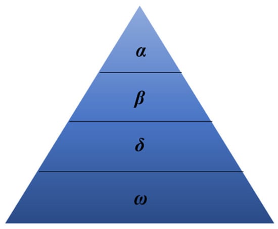
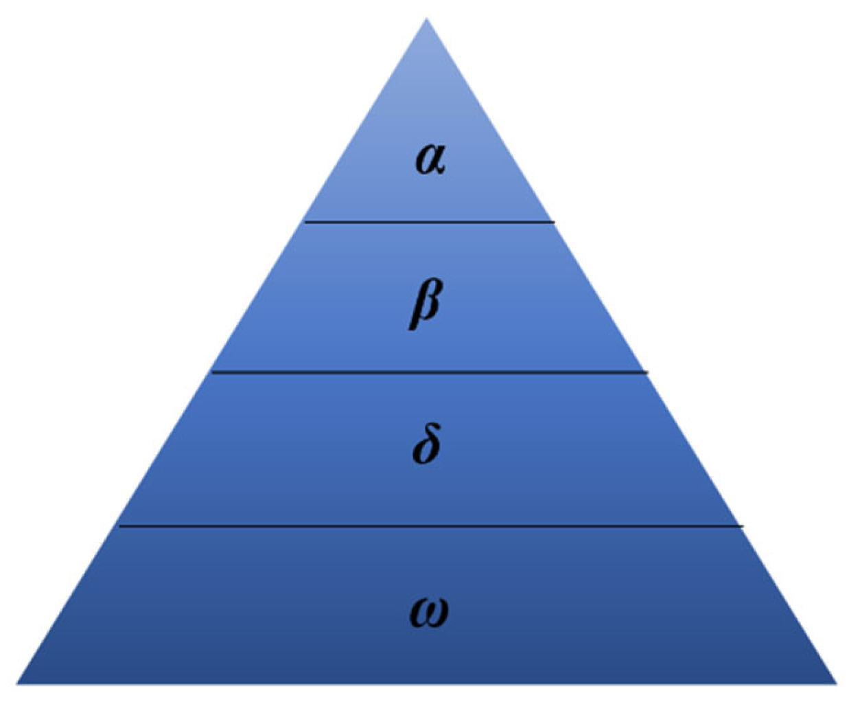
The Grey Wolf Optimizer (GWO) is a novel intelligent optimization algorithm. As illustrated in Figure 1, the algorithm defines a social hierarchy comprising four distinct roles, i.e., α, β, δ, and ω, and guides the search process by simulating the cooperative hunting strategy of grey wolf packs to approximate the global optimum. The GWO algorithm has some advantages, including straightforward principles, inherent parallelism, ease of implementation, minimal requirement for parameter tuning, strong generalization capability, and robust global search performance [17].

Figure 1. Social hierarchy of grey wolves (GWO).

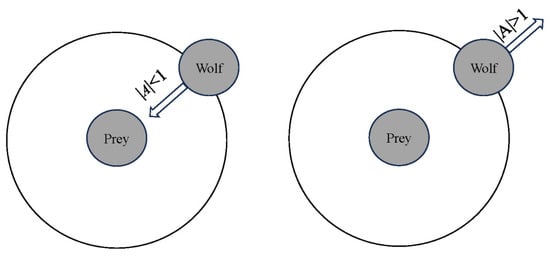
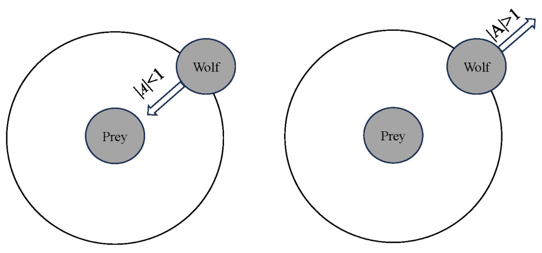
The Grey Wolf Optimizer primarily simulates three key hunting steps [26,27]: (1) encircling the prey; (2) hunting; and (3) attacking the prey. During the search process, the positions of individual wolves within the population are updated based on the positional information of the leadership hierarchy (i.e., α, β, and δ), enabling the swarm to progressively converge toward the optimal solution. This process can be mathematically represented by Equation (1). The convergence factor, i.e., a, decreases linearly from 2 to 0, which balances the algorithm’s global exploration and local exploitation capabilities. As illustrated in Figure 2, when |A| < 1, the algorithm tends toward local exploitation; when |A| > 1, it favors global exploration.

$$\left\{\begin{array}{c}D=\left|C·X_p-X\left(t\right)\right|\\ X\left(t+1\right)=X_p-A·D\\ A=2a·r_1-a\\ C=2r_2\end{array}\right.$$

(1)

where D represents the distance between the current wolf and the prey; t denotes the current iteration number; C and A are coefficient vectors; Xp and X are the position vectors of the prey and the grey wolf, respectively; r₁ and r₂ are random vectors within the interval [0, 1]; and a is the convergence factor. It is noted that the Grey Wolf Optimizer has been theoretically proven to converge under specific conditions. For example, Long et al. [28] provided a theoretical proof of convergence for the GWO and demonstrated that the algorithm is efficient, effective, and reliable for solving function optimization problems. Sun et al. [29] further analyzed the global convergence of the GWO using martingale theory and proved that the GWO algorithm can achieve global convergence with probability 1.

Figure 2. Schematic diagram of grey wolf position updating.

2.3. Convolutional Neural Network

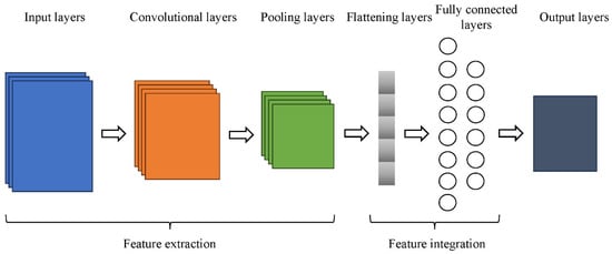
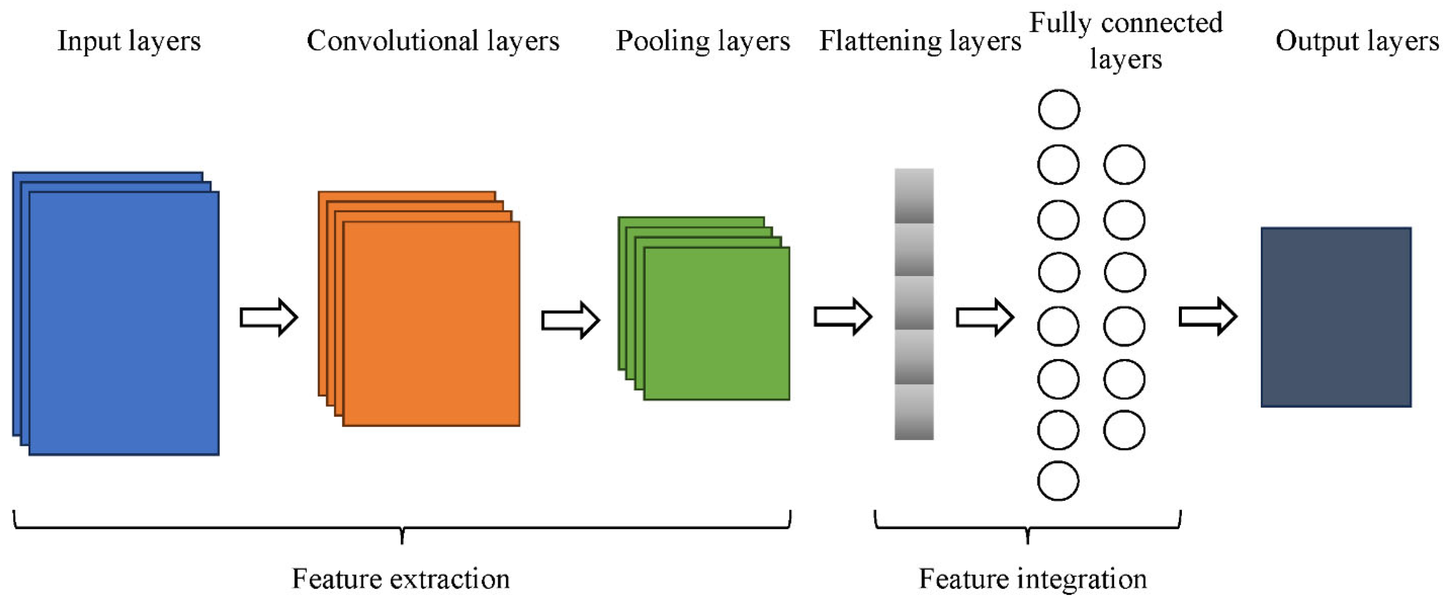
The Convolutional Neural Network (CNN) is a quintessential deep learning model whose architecture is inspired by the multilayer perceptron and is extensively applied in tasks such as image recognition and visual analysis. A typical CNN comprises several functional layers, as illustrated in Figure 3, primarily including input layers, convolutional layers, pooling layers (i.e., downsampling layers), fully connected layers, and output layers. The core of this architecture lies in the convolutional and pooling layers, which typically alternate. The computational process of the CNN is presented as follows: structured matrix data is first fed into the network through the input layer; subsequently, convolutional kernels or pooling windows perform calculations and shifting operations across the input data, enabling local feature perception and extraction to produce feature maps; and finally, the data processed by the convolutional and pooling layers is passed to the fully connected layers. These layers integrate the discriminative local information extracted from the preceding stages, ultimately yielding the data processed by the convolutional neural network.

Figure 3. Structure of the CNN model.

3. Construction of the VMD-GWO-CNN Model

3.1. Prediction Workflow

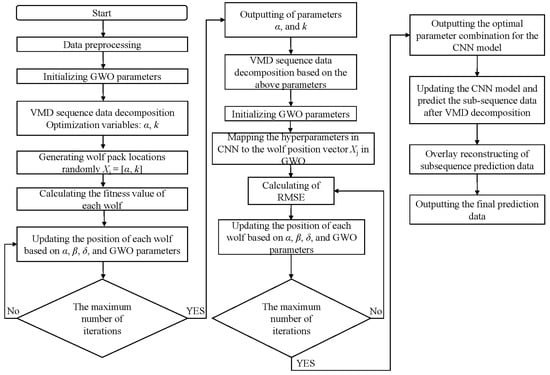
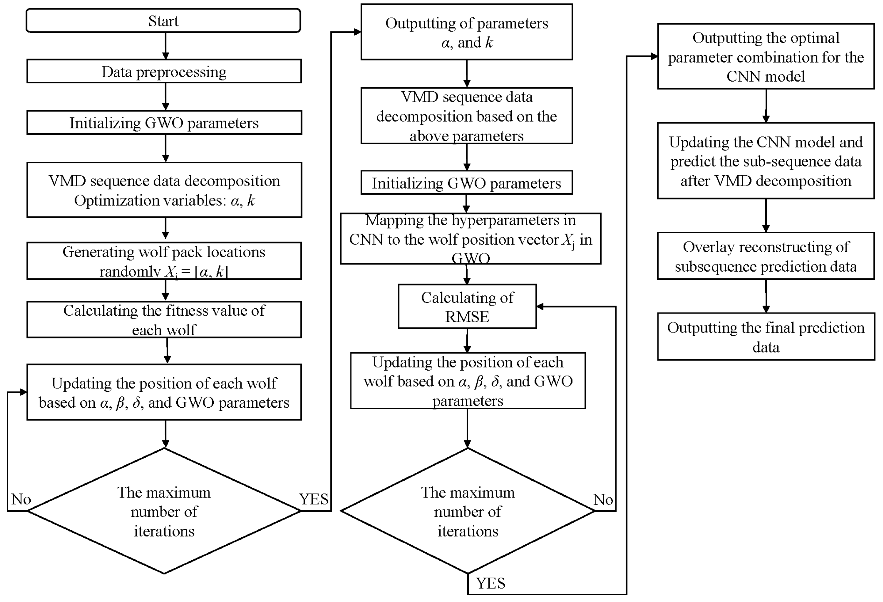
Based on the above theoretical foundations of machine learning prediction models, the VMD-GWO-CNN model is proposed. The operational workflow of the VMD-GWO-CNN model is illustrated in Figure 4 and the specific computational steps of the model are outlined as follows:

Figure 4. Workflow of the VMD-GWO-CNN hybrid model.

(1) Data Preprocessing: This stage includes data cleansing, linear interpolation, and normalization. Data cleansing removes outlier values and filters for representative data points. Due to the limited monitoring data in this study, it may lead to model overfitting or insufficient generalization capability. Thus, data augmentation is performed via linear interpolation based on findings from the literature [30]. This method suitably expands the dataset to meet the predictive requirements. Data normalization scales the data to a uniform magnitude and accelerates algorithmic convergence. The normalization formula is expressed as Equation (2):

$$x_n^{\ast }={\displaystyle \frac{x_n-x_{min}}{x_{max}-x_{min}}}$$

(2)

where $x_n^{\ast }$ denotes the normalized data; $x_n$ represents the original data; $x_{min}$ is the minimum value in the dataset; and $x_{max}$ is the maximum value.

(2) Optimization of VMD Parameter: First, the parameters of the GWO algorithm are initialized, including the wolf pack size, maximum iteration count, and the parameters a and ω. The VMD parameters, i.e., the penalty factor α and the number of modes k, are defined as the optimization variables. An objective function such as minimizing envelope entropy or sample entropy is adopted as the fitness function to evaluate the decomposition quality of VMD corresponding to each wolf’s position. The initial wolf positions Xi = [α, k] are randomly generated, and the fitness value of each wolf is calculated. Based on the position information of the α, β, and δ wolves as well as the GWO parameters, the optimal solution (i.e., α), sub-optimal solutions (i.e., β and δ), and general solutions (i.e., ω) are updated iteratively. The process is repeated until the termination criterion is met, at which point the optimal α and k are output.

(3) Optimization of CNN Hyper parameter: The optimized parameters α and k obtained from the previous steps are used to decompose the preprocessed data. The several Intrinsic Mode Function (IMF) components are obtained. The hyperparameters of the CNN such as the number of convolutional kernels and the learning rate are mapped to the wolf position vector Xj in the GWO framework. Then, the CNN model is trained by using the IMF component data and the GWO algorithm, thereby searching for the optimal combination of hyperparameters (e.g., time-step length and learning rate). Based on this, an update of the CNN model parameters is completed. The optimized CNN model is subsequently used to predict each VMD subsequence separately. The final prediction result is obtained by superimposing and reconstructing the predictions of all subsequences.

3.2. Introduction to Evaluation Indicators

To evaluate the predictive performance of the models, the following metrics are employed as evaluation criteria: Root Mean Square Error (RMSE), Mean Absolute Error (MAE), Mean Absolute Percentage Error (MAPE), and the Coefficient of Determination (R²). The definitions of these prediction evaluation metrics are listed in Table 1. In Table 1, n denotes the number of samples; y_i represents the actual value of the i-th sample; $y_i^{\prime }$ represents the predicted value of the i-th sample; and $\overline{y}$ denotes the mean of the actual values.

Table 1. Evaluation metrics.

Evaluation Metrics	Formulae of Evaluation Metrics	Notes
RMSE	$\sqrt{{\displaystyle \frac{1}{n}}{\displaystyle \sum _{i=1}^n{\left(y_i-{y^{\prime }}_i\right)}^2}}\in \left[0,+\infty \right)$	The smaller the value, the greater the predictive accuracy and the lower the average error magnitude.
MAE	${\displaystyle \frac{1}{n}}{\displaystyle \sum _{i=1}^n\left|y_i-{y^{\prime }}_i\right|}\in \left[0,+\infty \right)$
MAPE	${\displaystyle \frac{1}{n}}{\displaystyle \sum _{i=1}^n\left|\frac{y_i-{y^{\prime }}_i}{y_i}\right|}\times 100\%\in \left[0,+\infty \right)$
R2	$1-{\displaystyle \frac{{\displaystyle \sum _{i=1}^n{\left(y_i-{y^{\prime }}_i\right)}^2}}{{\displaystyle \sum _{i=1}^n{\left(y_i-{\overline{y}}_i\right)}^2}}}\in \left[0,1\right]$	The higher the value, the greater the predictive accuracy.

4. Engineering Case Study

4.1. Data Source

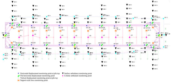
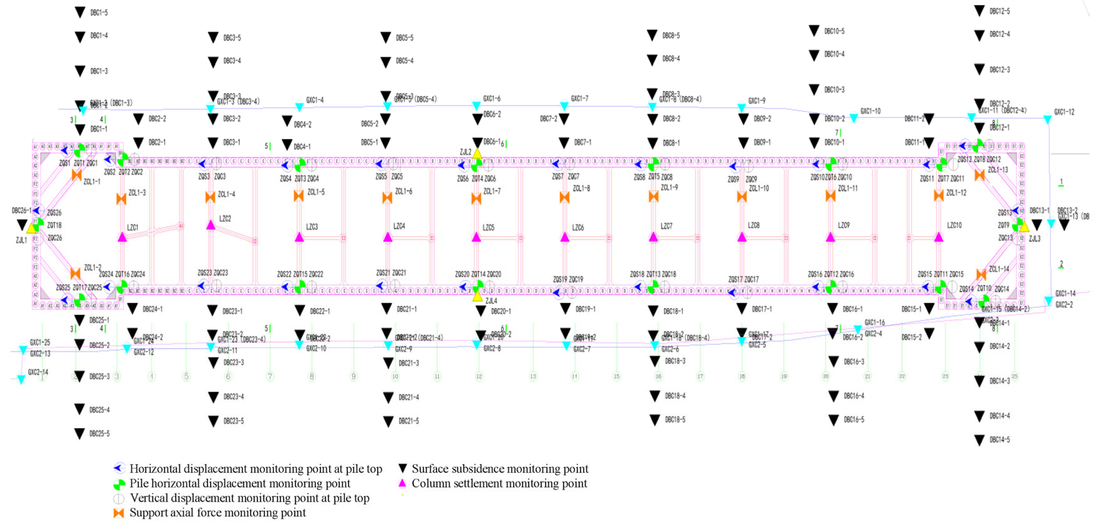
Taking the field monitoring data from Gangkoucun Station in the Wuhan Metro Line 12 as a case study, this analysis focuses on predictions for four different monitoring items, including ground settlements, horizontal and vertical displacements of pile top, and support axial forces. Figure 5 is the layout plan of the monitoring points. Among which the monitoring point numbers, i.e., DBC, ZQS, ZQC, and ZCL, present the ground settlements, horizontal displacements of pile top, vertical displacements of pile top, and support axial forces, respectively. For the aforementioned four distinct monitoring items, monitoring data corresponding to the four selected monitoring points are analyzed, i.e., DBC13-4, ZQS-15, ZQC-12, and ZCL1-6. The dataset covers the period from 30 November 2021 to 6 September 2022. Moreover, the excavation depth of the foundation pit is 17.4 m, and the buried depth of the groundwater level is 3.6 m. The foundation pit can be excavated in four stages, with each stage reaching a depth of 2 m, 5.3 m, 6.2 m, and 3.9 m, respectively. The supporting structure system comprises one reinforced concrete support and two steel pipe supports. In accordance with the data processing procedures described in Section 3.1, the monitoring data for each item underwent preprocessing, followed by decomposition using Variational Mode Decomposition (VMD). The processed data was then partitioned into training and testing sets, with the first 280 data points allocated for model training and the remaining 20 data points reserved for model validation and performance evaluation.

Figure 5. Layout plan of monitoring points.

The monitoring instruments and measurement accuracy corresponding to different monitoring items are presented, as shown in Table 2. Among them, the ground settlements, horizontal and vertical displacements of pile top, and support axial forces are measured by electronic level (Model: Trimble DINI03, Trimble Inc., Sunnyvale, CA, USA), total station (Model: IM-101, Sokkia, Tokyo, Japan), and steel bar dynamometer (Model: JY-1010, Golden Civil Engineering, Changzhou, China). The monitoring data were collected through manual on-site measurements, and the monitoring frequency was constrained by factors such as construction progress and labor costs, resulting in a limited volume of monitoring data. However, based on the research of Unterthiner et al. [31], the neural networks can learn effective representations from modest sample sizes when architecture and hyperparameters are carefully optimized. Therefore, Variational Mode Decomposition (VMD) was employed to decompose the original time series into multiple stationary subsequences (IMF components), effectively augmenting the feature space and reducing noise interference. Moreover, combined with the GWO-based hyperparameter optimization, the approach used in this study mitigated overfitting risks by ensuring that the model captured underlying patterns in the data.

Table 2. Monitoring instruments and measurement accuracy.

Monitoring Items	Monitoring Instruments	Model	Measurement Accuracy
Ground settlements	Electronic level	Trimble DINI03	±0.3 mm/km
Horizontal displacements of pile top	Total station	IM-101	1″/1.5 + 2 ppm
Vertical displacements of pile top	Total station	IM-101	1″/1.5 + 2 ppm
Support axial forces	Steel bar dynamometer	JY-1010	±0.5% F.S.

4.2. Data Decomposition Based on VMD

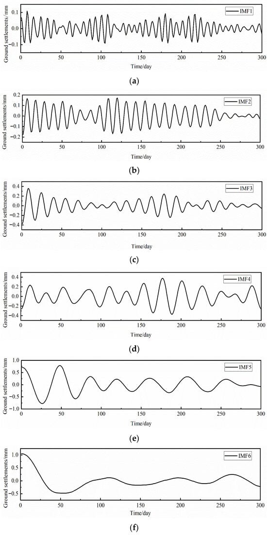
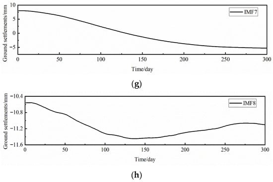
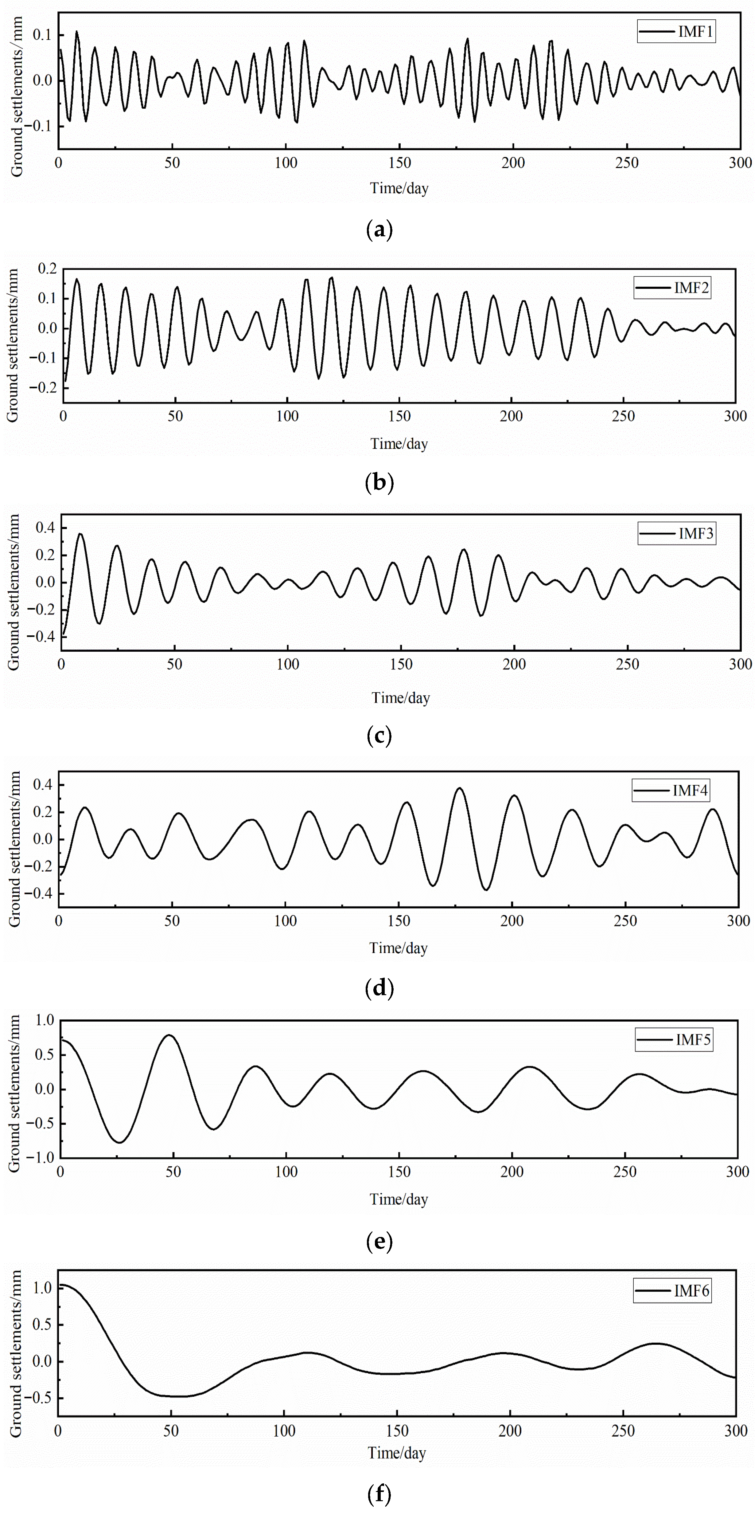
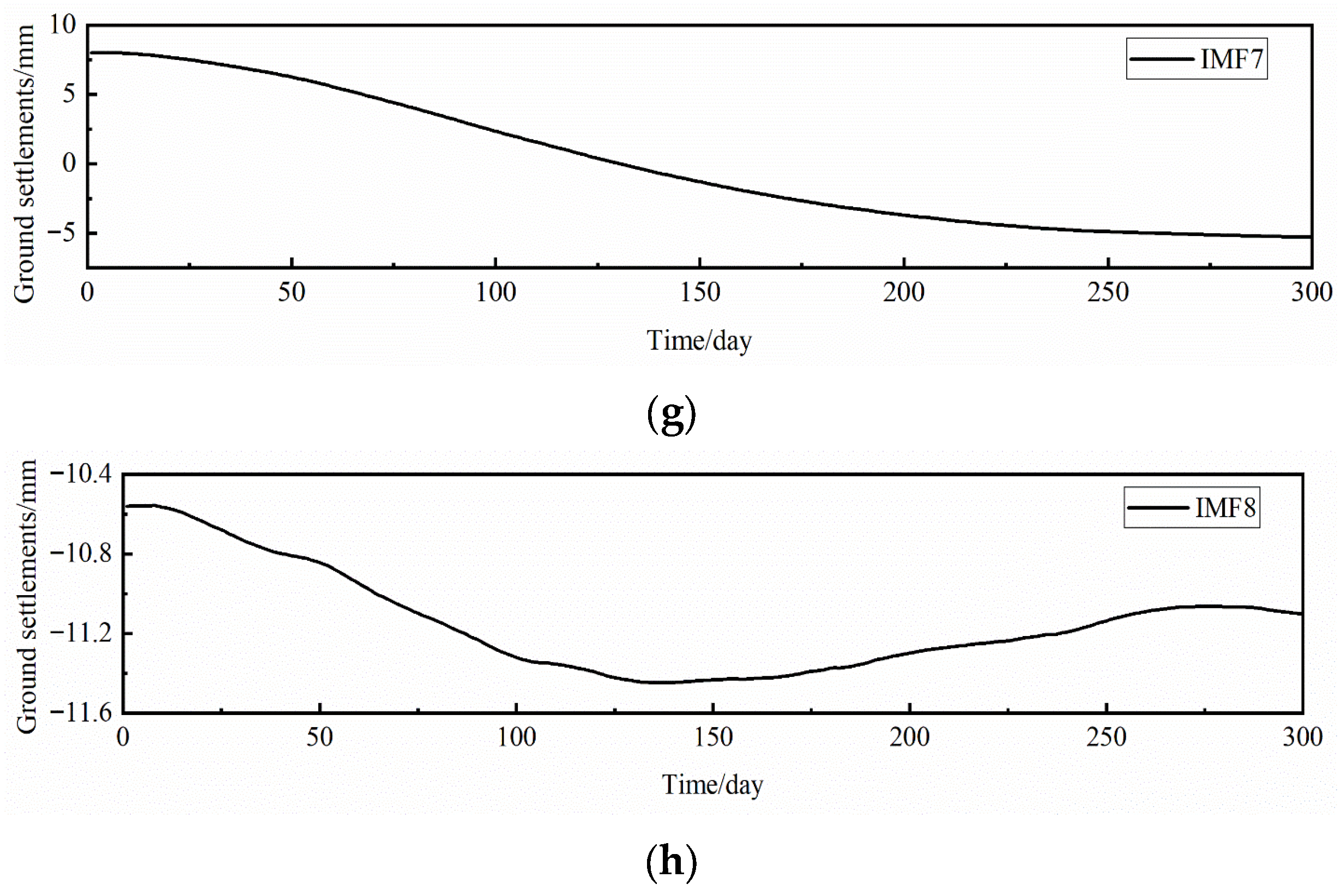
Taking the data from monitoring point DBC13-4 as an example, VMD was employed to decompose the ground settlement time series. As the performance of VMD critically depends on the appropriate selection of two key parameters, i.e., the penalty factor (α) and the number of modes (k), a rigorous analysis for determining their optimal values was conducted. The Grey Wolf Optimizer (GWO) was applied to optimize the parameters α and k for VMD. Based on the studies of Long et al. [32], the GWO parameters were configured as follows: a population size of 30 and a maximum iteration count of 20. Moreover, the search ranges for the penalty factor α and the number of modes k were set to [100, 3000] and [3, 12], respectively. The choice of the mode number k is critical because the smaller k value leads to under-decomposition, while the larger k value leads to over-decomposition. To address this trade-off, some researchers typically define a reasonable search space that encompasses the potential optimal k values for most signals. For example, Li et al. [33] explicitly states in their study on VMD parameter optimization that the original signal may be decomposed by VMD as the k value is varied from 2 to 10. This establishes that varying k values within the range of 2 to 10 is a well-accepted practice in VMD applications. The range [3, 12] adopted in this study aligns with and slightly extends this common practice, allowing the GWO algorithm to efficiently search for the optimal k without venturing into regions where decomposition quality deteriorates or computational cost becomes prohibitive. Following the optimization process for the VMD parameters illustrated in Figure 4, the optimal parameters were obtained, i.e., α = 800, and k = 8. The preprocessed monitoring data from DBC13-4 are decomposed via VMD using the above optimal parameters, resulting in eight Intrinsic Mode Function (IMF) components with distinct physical interpretations. Figure 6 shows the decomposition results of monitoring data from DBC13-4 based on VMD. Among that, Figure 6a–h are presented as eight different components. As seen, the time-frequency characteristics of each IMF component are presented. The different components distinctly reflect various deformation characteristics during the excavation process. For example, the curves of IMF7 and IMF8 exhibit relatively gentle variations and long periods, meaning that the excavation is completed, and the surface subsidence is stabilized. The curves of IMF4 to IMF6 demonstrate similar variation patterns with minor fluctuations and can be interpreted as periodic displacements primarily influenced by staged construction activities. In contrast, the curves of IMF1 to IMF3 display higher-frequency fluctuations with less apparent regularity, likely attributable to stochastic disturbances caused by weakly correlated factors such as human operational variability.

Figure 6. VMD decomposition results of monitoring data from DBC13-4: (a) IMF-1; (b) IMF-2; (c) IMF-3; (d) IMF-4; (e) IMF-5; (f) IMF-6; (g) IMF-7; (h) IMF-8.

Likely, the same methodology is applied to the other three monitoring items, including horizontal and vertical displacements of pile top and support axial forces. The optimal parameters for VMD of the above monitoring items can be obtained. The search ranges for the penalty factor (α) and the number of modes (k) are set consistent with those for the ground settlement. Following the optimization procedure, the optimal parameters for various monitoring items are obtained. The penalty factor (α) for horizontal and vertical displacements of pile top and support axial force are 1200, 600, and 2000, respectively, and the corresponding number of modes (k) is 8 for various monitoring items.

4.3. Comparative Analysis of Prediction Results

The optimized VMD parameters for the four monitoring items are used to decompose the time-series data for ground settlement (i.e., DBC13-4), horizontal displacement of pile top (ZQS-15), vertical displacement of pile top (ZQC-12), and support axial force (ZCL1-6). The eight IMF components for each monitoring item are obtained. For each component, the first 280 data points are used as the training set and the subsequent 20 points as the test set. The VMD-GWO-CNN model is applied to predict each component series. The final prediction values for different monitoring items are obtained by superimposing the predicted values of all components, followed by denormalization. This process successfully generated 20-day-ahead predictions for the four monitoring items during the excavation period. Moreover, three machine learning models, i.e., LSTM, CNN, and GWO-CNN model, are employed to predict the same monitoring data. Their results are compared with those of the VMD-GWO-CNN model to validate the reliability and superiority of the latter. In accordance with the hyperparameter search spaces recommended in the studies of Chai et al. [25] and Li et al. [26], the hyperparameters of the CNN model were selected for optimization and their corresponding value ranges are specified in Table 3.

Table 3. Optimization ranges for hyperparameters.

Hyperparameters	Value Ranges
Learning Rate	[8.5 × 10−3, 2 × 10−2]
Batch_Size	[8, 256]
Optimizer	[Adam, RMSprop, SGD]
Dropout_Size	[0.25, 0.5]
Kernel Size	[3 × 3, 5 × 5, 7 × 7]

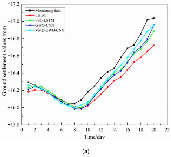
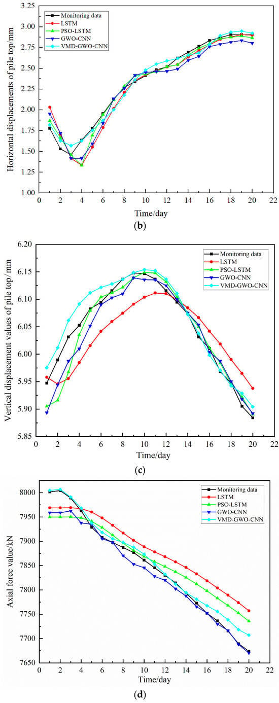
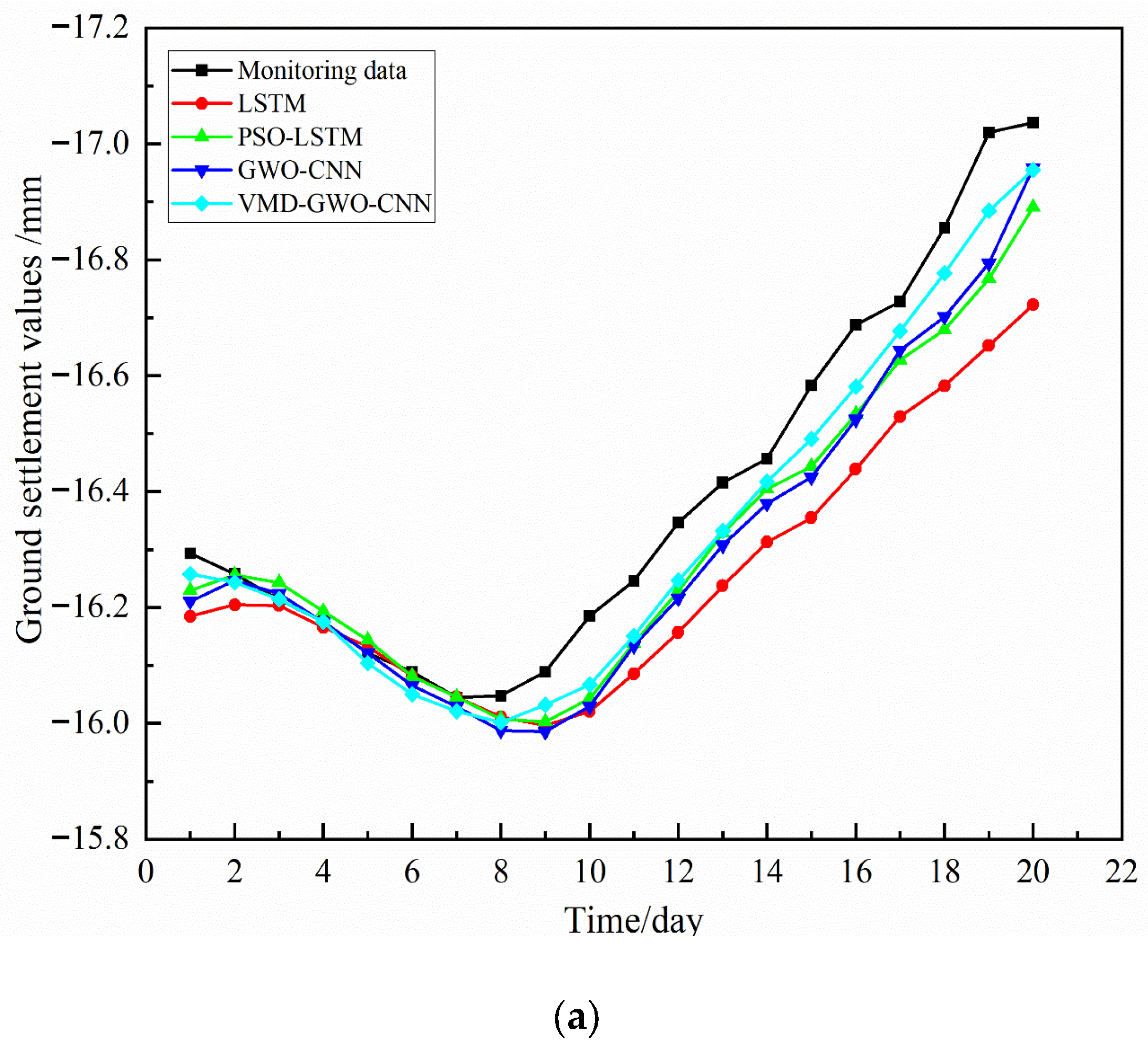
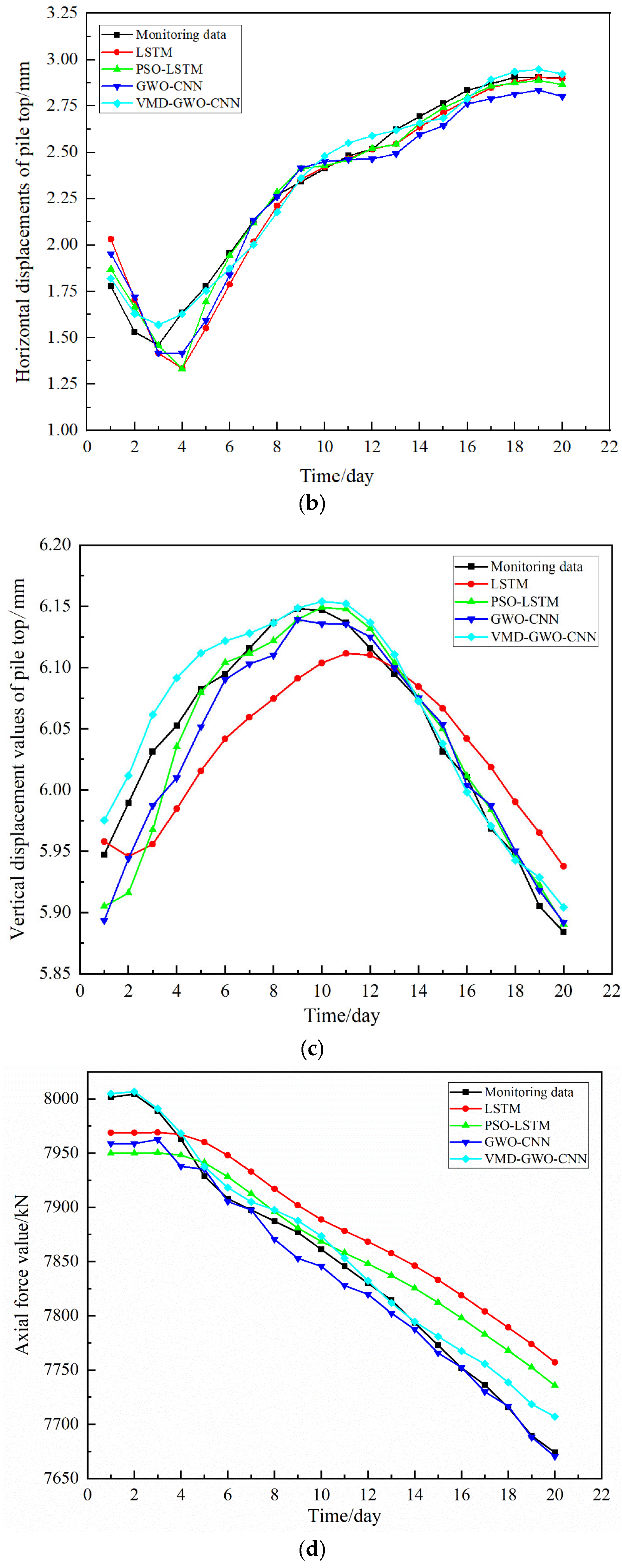
The hyperparameters of the CNN model via the GWO algorithm are optimized, and the optimal hyperparameters for each IMF component across all monitoring items are obtained. Each corresponding model is then trained using the training set and subsequently validated and analyzed with the test set. The prediction curves of the models on the test set are shown in Figure 7. Among them, Figure 7a–d represent the results of ground settlements (DBC13-4), horizontal displacements of pile top (ZQS-15), vertical displacements of pile top, and support axial forces (ZCL1-6), respectively. As seen, the predictive curves corresponding to various models (i.e., LSTM, CNN, GWO-CNN and VMD-GWO-CNN) exhibit consistent trends and align with the patterns observed in the monitoring data for different monitoring items. The phenomena demonstrate that all four models can effectively predict the four types of monitoring data, including ground settlements, horizontal and vertical displacements of pile top, and support axial forces. By integrating the Grey Wolf Optimizer (GWO) and Variational Mode Decomposition (VMD) techniques to decompose the original monitoring data into multiple stationary subsequences, the VMD-GWO-CNN model significantly enhances the expressiveness of data features. Consequently, it exhibits the best predictive performance across all four monitoring categories.

Figure 7. Comparative performance of different models on monitoring datasets: (a) ground settlements (DBC13-4); (b) horizontal displacements of pile top (ZQS-15); (c) vertical displacements of pile top (ZQC-12); (d) support axial forces (ZCL1-6).

Based on the evaluation metrics outlined in Table 1, the corresponding indicator values for the different prediction models are calculated, as presented in Table 4. As seen, the VMD-GWO-CNN model achieves the best performance metrics in predicting all four monitoring datasets. To illustrate the predictive superiority of the VMD-GWO-CNN model, an analysis using the RMSE values from Table 4 is provided. For ground settlements, the RMSE of the VMD-GWO-CNN model is 0.0723 mm, representing a significant reduction of 59.2%, 34.1%, and 33.0% compared to the LSTM, CNN, and GWO-CNN models, respectively. For horizontal displacements of pile top, the RMSE of 0.0648 mm is 46.9%, 24.0%, and 42.1% lower than those of the LSTM, CNN, and GWO-CNN models. For vertical displacements of pile top, the model’s RMSE is 0.0195 mm, showing reductions of 59.2%, 24.7%, and 20.4% compared to the other three models. The VMD-GWO-CNN model also demonstrates exceptional performance in the prediction of support axial forces, with a RMSE of only 13.9419 kN, corresponding to substantial error reductions of 71.6%, 61.8%, and 25.9% relative to the LSTM, CNN, and GWO-CNN models. Furthermore, the VMD-GWO-CNN model consistently outperforms all comparative models across the other three evaluation metrics, i.e., MAE, MAPE, and R², demonstrating comprehensive and stable predictive capability. These results robustly validate the significant advantage of the VMD-GWO-CNN model in multi-parameter deformation prediction for deep excavations, offering more reliable technical support for engineering safety monitoring.

Table 4. Comparison of various models across evaluation metrics.

Model	Monitoring Point	RMSE	MAE	MAPE (%)	R2
VMD-GWO-CNN	DBC13-4	0.0723	0.0607	0.37	0.9460
	ZQS-15	0.0648	0.0546	2.58	0.9821
	ZQC-12	0.0195	0.0159	0.26	0.9418
	ZCL1-6	13.9419	10.7298	0.14	0.9806
GWO-CNN	DBC13-4	0.1080	0.0878	0.53	0.8795
	ZQS-15	0.1119	0.0945	4.52	0.9466
	ZQC-12	0.0245	0.0185	0.31	0.9074
	ZCL1-6	18.8084	13.5711	0.17	0.9648
CNN	DBC13-4	0.1097	0.0874	0.53	0.8756
	ZQS-15	0.0853	0.0520	2.69	0.9689
	ZQC-12	0.0259	0.0168	0.28	0.8971
	ZCL1-6	36.5013	31.0669	0.40	0.8673
LSTM	DBC13-4	0.1772	0.1399	0.84	0.6754
	ZQS-15	0.1222	0.0834	4.42	0.9362
	ZQC-12	0.0478	0.0428	0.71	0.6490
	ZCL1-6	49.0744	44.2224	0.57	0.7602

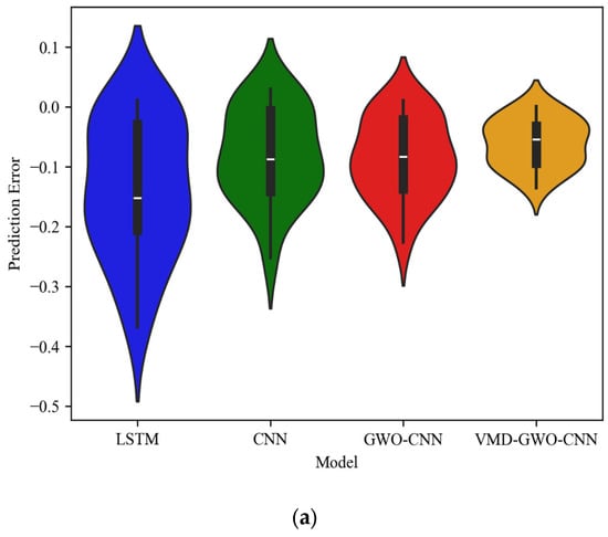
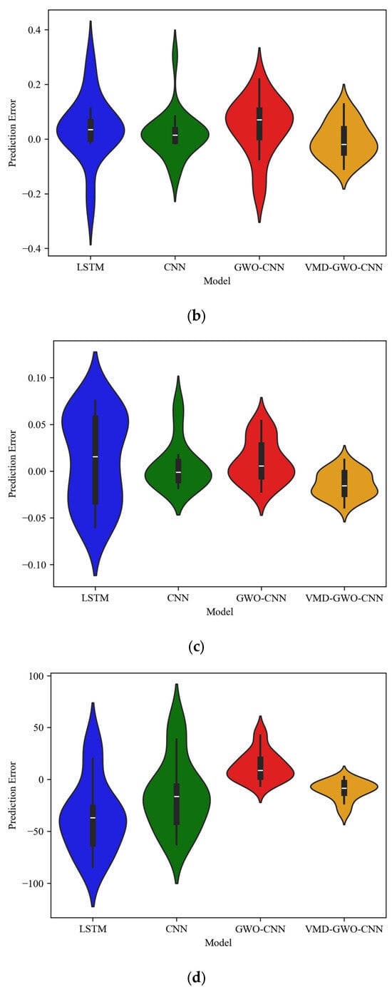
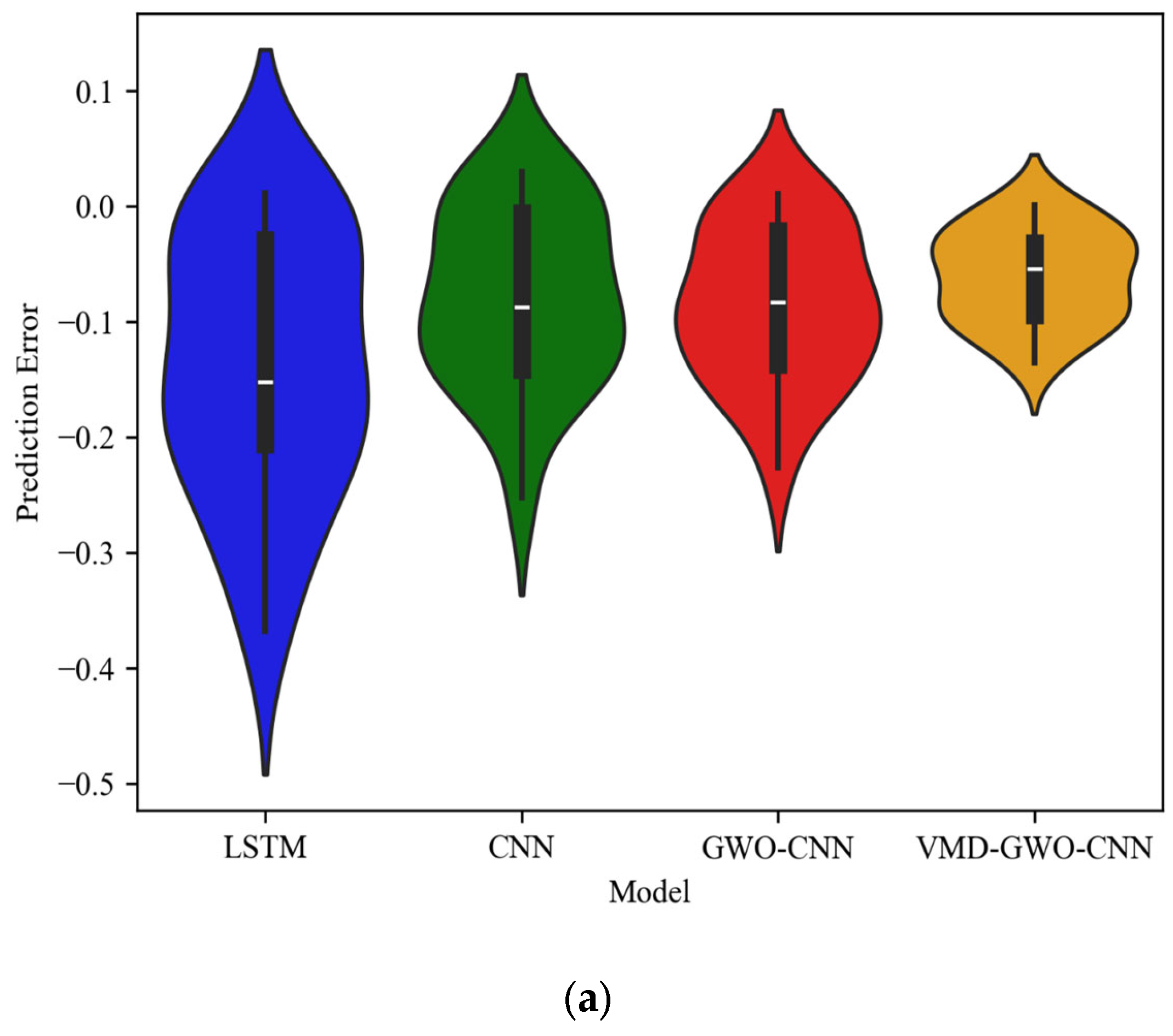
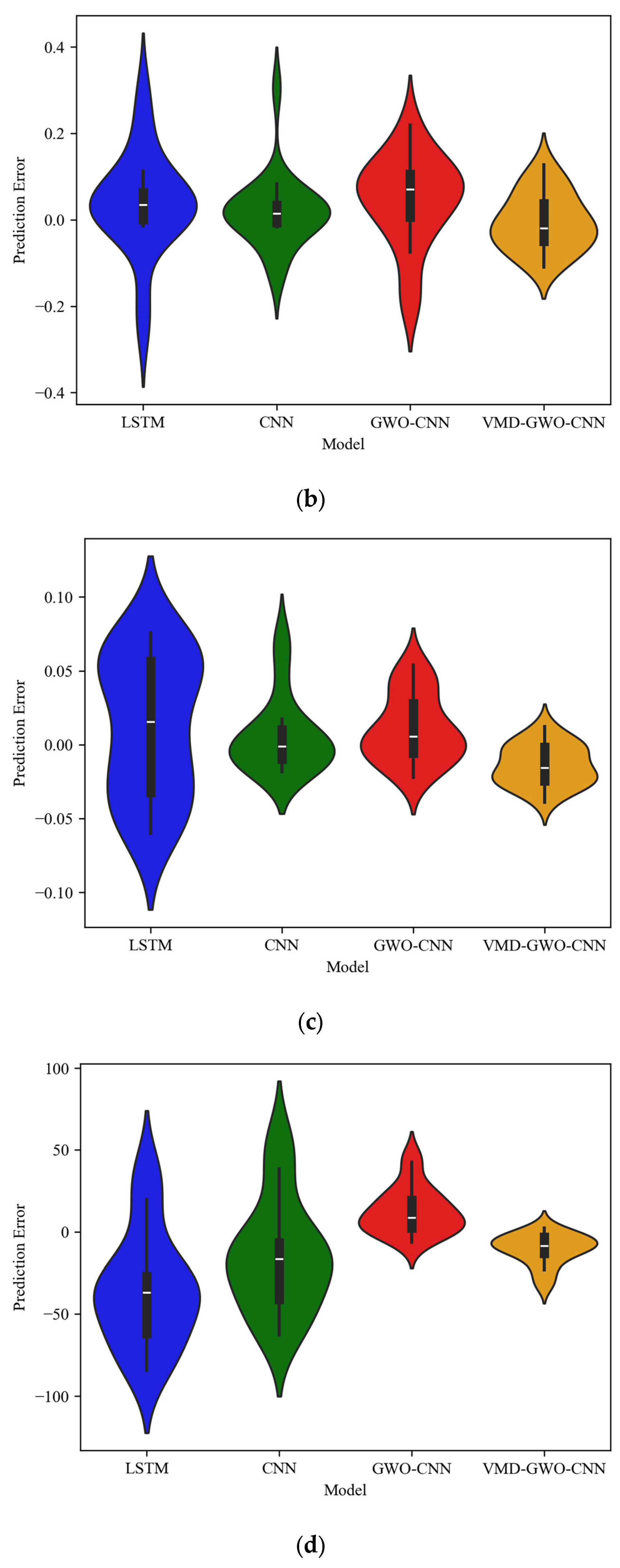
Table 4 shows an overview of the overall performance of each model but does not describe the specific distribution of errors. In contrast, the error distribution offers a more intuitive visualization of the error density and range for the different models, thereby enabling a deeper understanding of their predictive capabilities. Figure 8 shows the error distribution of different machine learning models (including LSTM, CNN, GWO-CNN, and VMD-GWO-CNN) for various monitoring items: Figure 8a–d represent the results of ground settlements (DBC13-4), horizontal displacements of pile top (ZQS-15), vertical displacements of pile top (ZQC-12), and support axial forces (ZCL1-6), respectively. Taking the error distribution of ground settlements as an example, i.e., Figure 8a, the prediction capabilities for different models are analyzed. As can be observed, the LSTM model exhibits the most dispersed error distribution, with extreme values ranging from −0.37 to 0.01 and a mean around −0.15. In addition, it presents the longest error bars, indicating a pronounced systematic bias and poor prediction stability. Compared with LSTM, the CNN model shows a more concentrated error distribution, mainly within the range of −0.25 to 0.02, with a mean close to −0.10, demonstrating an overall improvement in predictive performance. After introducing the GWO optimization, the GWO-CNN model exhibits a further reduction in error dispersion, with the primary error interval narrowed to approximately −0.20 to 0, accompanied by a shorter error bar. This suggests that swarm intelligence optimization effectively enhances network parameter searching, thereby improving both prediction accuracy and stability. In contrast, the VMD-GWO-CNN model presents the most compact violin shape, with errors predominantly concentrated within the narrow range of −0.12 to 0. Its mean value is closest to zero and it exhibits the shortest error bars among all models, indicating not only the lowest systematic bias but also the highest consistency in prediction results. Overall, the synergistic integration of VMD decomposition and GWO optimization effectively suppresses noise in the original signal and enhances model performance, enabling the VMD-GWO-CNN model to achieve significantly superior accuracy and robustness compared with the other benchmark models.

Figure 8. The error distribution of different machine learning models for various monitoring items: (a) ground settlements (DBC13-4); (b) horizontal displacements of pile top (ZQS-15); (c) vertical displacements of pile top (ZQC-12); (d) support axial forces (ZCL1-6).

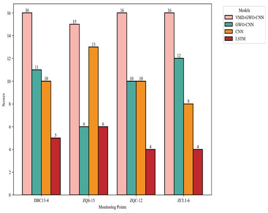
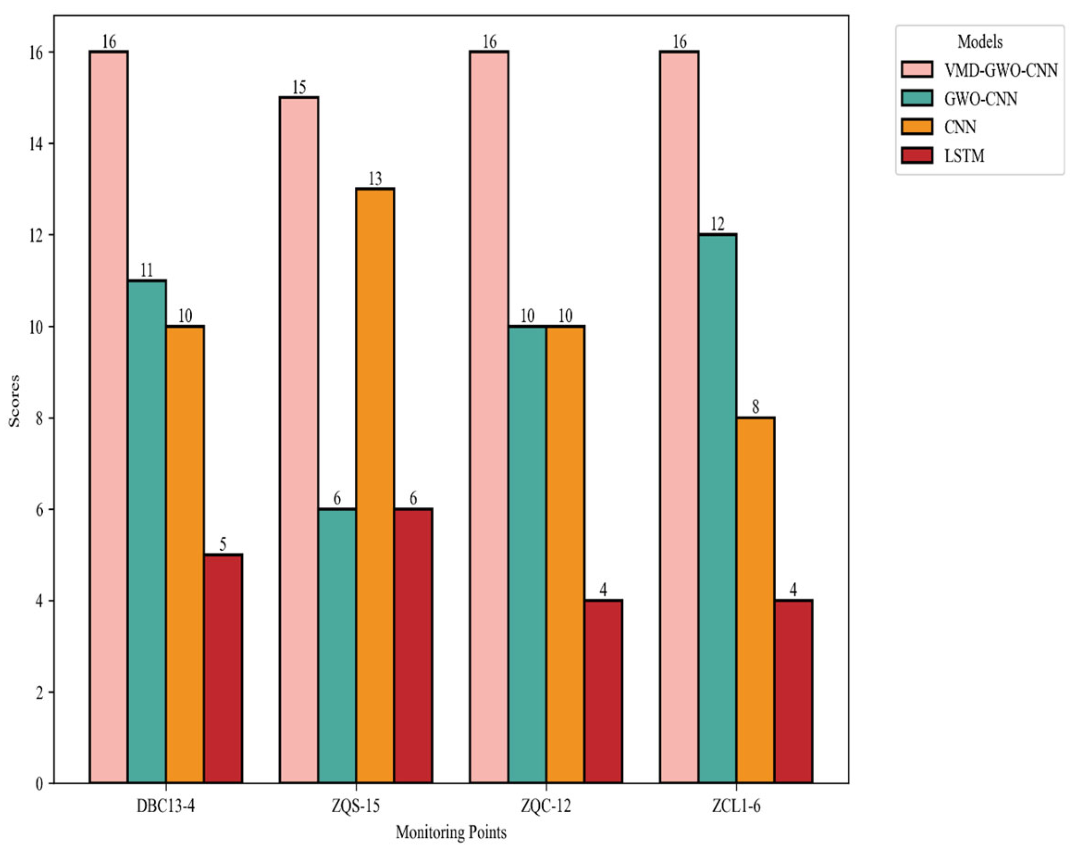
In addition, based on the decision-making methodology derived from existing research, the various models are scored and ranked. For each evaluation metric, the best-performing algorithm receives four points, followed by three points, then two points, and the weakest receives one point. If multiple algorithms yield identical results for a given metric, they are assigned the same score. The maximum possible score is 16 with four evaluation metrics in total, in which a higher score indicates better predictive performance. Thus, Figure 9 shows the scores of different prediction models. Among all monitoring items, the VMD-GWO-CNN model achieves the highest score. Using ground settlement as a case study (i.e., DBC 13-4), the scoring results of different prediction models are further analyzed: the VMD-GWO-CNN model achieves the highest score (16 points), demonstrating the best performance, followed by the GWO-CNN model (11 points), and then the CNN model (10 points). The LSTM model ranks last with the lowest score (5 points).

Figure 9. Scores of different prediction models.

In summary, the aforementioned analysis demonstrates that the VMD-GWO-CNN model exhibits the best overall predictive performance across various monitoring items, including ground settlements (i.e., DBC13-4), horizontal displacements of pile top (ZQS-15), vertical displacements of pile top (ZQC-12), and support axial forces (ZCL1-6).

5. Discussion

It is noted that the predicted values of support axial force exhibit a systematic overestimation in the later stage shown in Figure 7d. This deviation may be attributed to the inherent “information gap” of univariate prediction models. A comparison with the study by Chen et al. [34] suggests that the present model fails to incorporate four key physical variables, i.e., diaphragm wall inclinometer readings [35], upright rebound [36], excavation depth [37], and ambient temperature [38]. Moreover, the employed steel stress meter measurement method is sensitive to temperature variations; fluctuations in ambient temperature directly affect the meter readings, introducing temperature-induced variations into the measured axial force values. Since the model does not account for the coupling effects of environmental factors like temperature, its predictions tend to follow earlier trends and fail to capture the actual force increase resulting from multi-factor interactions, leading to the observed deviation from the measured data.

In addition, recalling previous studies, some scholars have conducted extensive research on predicting ground displacement induced by excavation, including empirical formulas, theoretical analysis, and numerical simulation. These approaches can reveal the mechanical interaction between excavation and the surrounding soil, and preliminarily reflect the influence of soil constitutive relationships on displacement; however, their application is constrained by several inherent challenges, i.e., the difficulty in accurately determining soil constitutive parameters, the high computational cost of numerical procedures, the complexity of theoretical derivations, and generally low operational efficiency. The integrated VMD-GWO-CNN-based machine learning model developed in this study effectively addresses these limitations. In this model, the Grey Wolf Optimizer (GWO) is used to synchronously and intelligently optimize the critical parameters of Variational Mode Decomposition (VMD), i.e., the penalty factor (α) and the number of modes (k), alongside the hyperparameters of the Convolutional Neural Network (CNN). In this way, it represents a significant enhancement in the engineering application efficiency for predicting ground displacement in subway deep excavation projects.

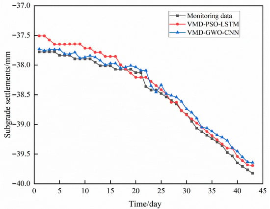
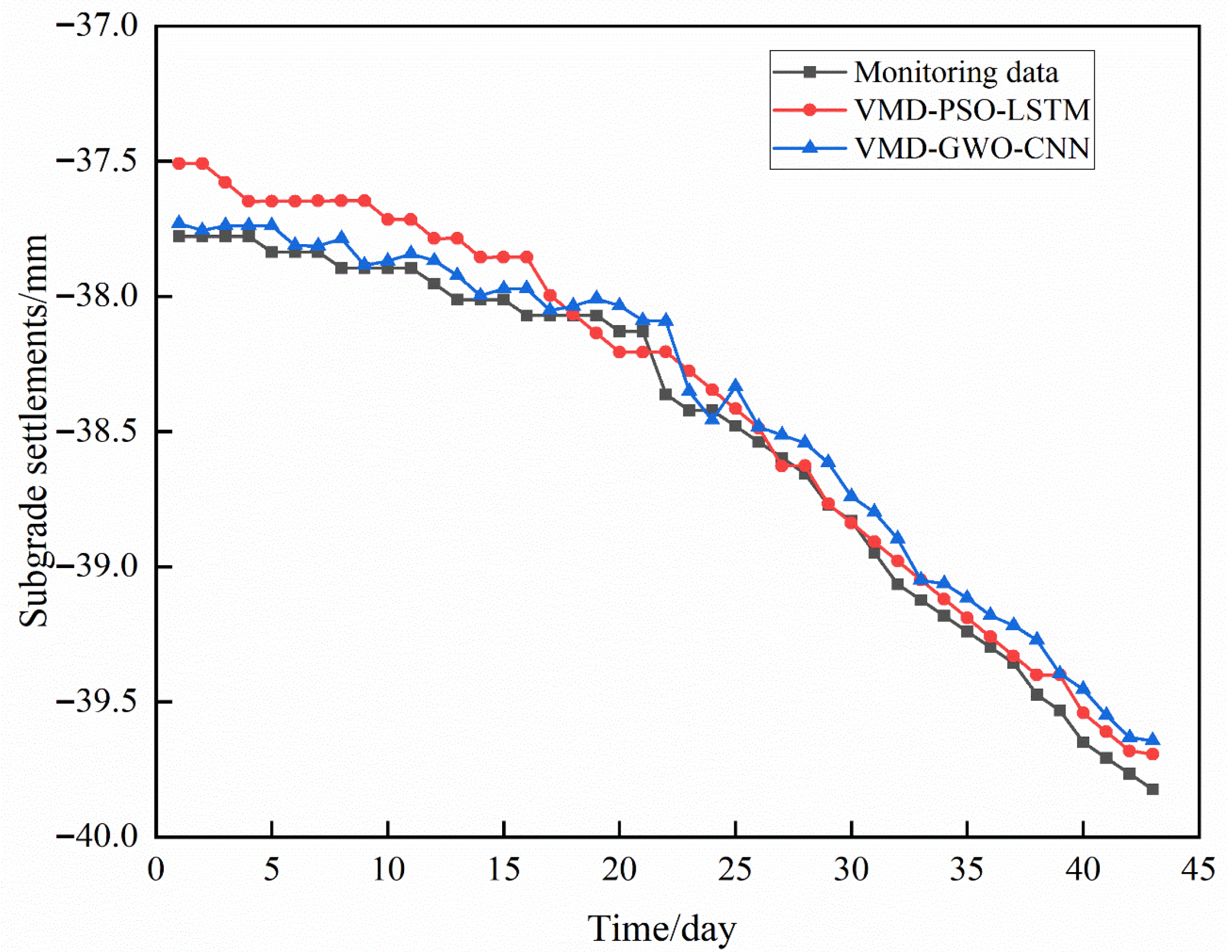
In addition, to further validate the applicability of the proposed model, the hybrid framework is applied to the predictive analysis of monitoring data from various engineering types. Figure 10 shows the predicted results of the VMD-GWO-CNN model at monitoring point No. 4 of the high-fill subgrade settlement. As seen, both the VMD-GWO-CNN model and the VMD-PSO-LSTM model employed by Chai et al. [25] exhibit good predictive ability. The predicted results are close to the monitored data. However, the proposed model (i.e., the VMD-GWO-CNN model) achieves better evaluation metrics compared with those from the VMD-PSO-LSTM model. The RMSE, MAPE, and R² values of the VMD-GWO-CNN model are 0.1103, 0.24%, and 0.9719, while the corresponding values of the VMD-PSO-LSTM model are 0.4496, 1.07%, and 0.9141. The above results demonstrate the superior performance of the proposed model compared to the VMD-PSO-LSTM model.

Figure 10. Application of the VMD-GWO-CNN model in high-fill subgrade settlement.

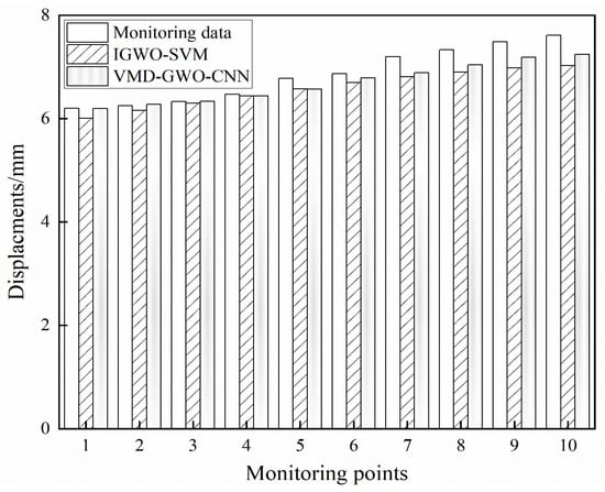
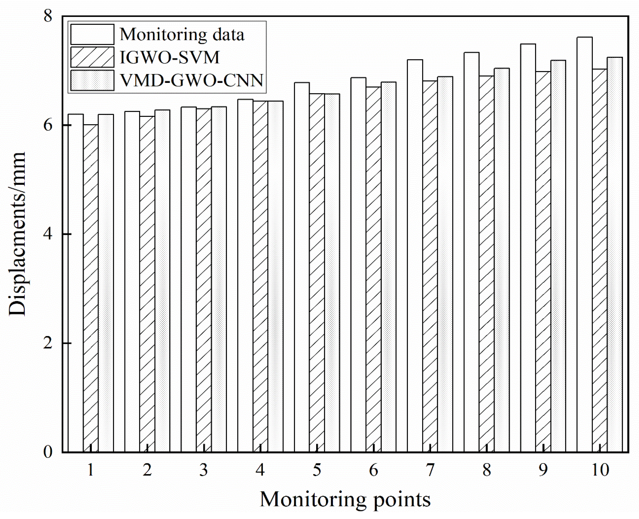
Furthermore, the applicability of the proposed model is analyzed in slope displacement. Figure 11 shows the predicted results of the VMD-GWO-CNN model at a high-speed railway tunnel portal. As seen, both the VMD-GWO-CNN model and the IGWO-SVM model used by Liu et al. [39] can perform good predictions in slope displacement. However, the proposed model yields a RMSE of 0.2141 and a MAPE of 2.25% for the slope displacement monitoring data. Among that, the RMSE is comparable to that reported in reference [39], i.e., 0.21, and the MAPE shows a slight improvement compared to 2.41%. This further verifies the effectiveness of the proposed model in slope deformation monitoring.

Figure 11. Application of the VMD-GWO-CNN model in slope displacement.

6. Conclusions

A hybrid prediction model integrating Variational Mode Decomposition (VMD), the Grey Wolf Optimizer (GWO), and the Convolutional Neural Network (CNN), termed VMD-GWO-CNN, is constructed to predict various monitor items. Among that, the monitoring data from the foundation pit at Gangkoucun Station on Wuhan Metro Line 12 is used. The main conclusions are as follows:

(1) The application of VMD decomposes the original monitoring data into multiple stationary subsequences, mitigating noise interference. Moreover, the GWO algorithm intelligently optimizes the key parameters of VMD as well as the hyperparameters of the CNN, ensuring optimal decomposition quality and model architecture. The optimization results indicate that the optimal VMD parameter combinations for the four different monitoring projects effectively balance the completeness of the modal components and reduce the noise present in the original data. Simultaneously, the prediction accuracy is improved by optimizing the hyperparameters of CNN using the GWO.

(2) The predicted results obtained by the VMD-GWO-CNN model are compared with those from different machine learning methods. Furthermore, the prediction results of the VMD-GWO-CNN model are consistent with those obtained from other machine learning-based methods. From four different evaluation indicators, it is evident that the proposed model exhibits superior predictive ability across four distinct monitoring items.

(3) The applicability of the VMD-GWO-CNN model in other geotechnical engineering projects has also been analyzed. In predicting high-fill embankment settlement, the VMD-GWO-CNN model yields superior results for monitoring point No. 4 compared to the VMD-PSO-LSTM model used in the reference. For slope displacement monitoring, the accuracy of the VMD-GWO-CNN model is significantly higher than that of the IGWO-SVM model. These findings indicate that the VMD-GWO-CNN model is applicable to deformation prediction in both slope engineering and subgrade engineering.

Various interpolation techniques exist for handling nonlinear data [40], including polynomial interpolation and spline interpolation. However, linear interpolation was still employed for data augmentation in this study. Based on the research results of Armstrong et al. [41], the reliability and simplicity of linear interpolation as a traditional method have been long validated in the engineering field. Besides that, the linear interpolation method can offer significant advantages in computational efficiency and simplicity, making it particularly suitable for engineering applications that may require rapid model updates to support on-site decision-making. In future research, the author will attempt to expand the data using different interpolation methods to verify the reliability of the model. Moreover, the current model relies solely on a single signal from historical monitoring data and cannot capture the coupling effects of other key physical variables (i.e., excavation depth and groundwater), resulting in predictions that lack explanatory power in terms of physical mechanisms. This is due to the lack of corresponding information on construction sequence and monitoring data, and the duration of each construction process cannot be fully determined. In the future, the authors will develop multivariate prediction frameworks that integrate multi-source physical variables into the input space. By enriching the data with key influencing factors, such models can learn the complex relationships between construction activities, environmental conditions, and structural responses, thereby improving both the prediction accuracy and physical interpretability of model.

References

- Anatolii, O.; Maksim, P.; Ivan, D.; Bashmakov, I. Determination of the bending moment in the diaphragm wall by in clinometric observations. In E3S Web of Conferences; EDP Sciences: Les Ulis, France, 2023; Volume 371. [Google Scholar]
- Xiao, H.J.; Zhou, S.H.; Sun, Y.Y. Wall deflection and ground surface settlement due to excavation width and foundation pit classification. KSCE J. Civ. Eng. 2019, 23, 1537–1547. [Google Scholar] [CrossRef] [Scilit]
- Zou, D.L.; Wu, L.L.; Hao, Y.F.; Xu, L.; Chen, J.J. Composition strength relationship study of ultrahigh performance fiber reinforced concrete (UHPFRC) using an interpretable data-driven approach. Constr. Build. Mater. 2023, 392, 131973. [Google Scholar] [CrossRef] [Scilit]
- Wang, M.; Zhao, G.; Liang, W.; Wang, N. A comparative study on the development of hybrid SSA-RF and PSO-RF models for predicting the uniaxial compressive strength of rocks. Case Stud. Constr. Mater. 2023, 18, e02191. [Google Scholar] [CrossRef] [Scilit]
- Karim, R.; Islam, M.H.; Datta, S.D.; Kashem, A. Synergistic effects of supplementary cementitious materials and compressive strength prediction of concrete using machine learning algorithms with SHAP and PDP analyses. Case Stud. Constr. Mater. 2024, 20, e02828. [Google Scholar] [CrossRef] [Scilit]
- Nguyen, H.; Vu, T.; Vo, T.P.; Thai, H.T. Efficient machine learning models for prediction of concrete strengths. Constr. Build. Mater. 2021, 266, 120950. [Google Scholar] [CrossRef] [Scilit]
- Kashem, A.; Karim, R.; Malo, S.C.; Das, P.; Datta, S.D.; Alharthai, M. Hybrid data-driven approaches to predicting the compressive strength of ultra-high-performance concrete using SHAP and PDP analyses. Case Stud. Constr. Mater. 2024, 20, e02991. [Google Scholar] [CrossRef] [Scilit]
- Wang, L.; Gao, F. Application research of time series-BP neural network in foundation pit engineering. Geomat. Spat. Inf. Technol. 2018, 41, 201–205. [Google Scholar]
- Donaldson, R.G.; Kamstra, M. An artificial neural network-GARCH model for international stock return volatility. J. Empir. Financ. 1997, 4, 17–46. [Google Scholar] [CrossRef] [Scilit]
- Zhao, Y.; Zhang, J.; Li, H. Deformation prediction analysis of vertical displacement of deep foundation pit based on LIBSVM. In E3S Web of Conferences; EDP Sciences: Les Ulis, France, 2020; Volume 206, p. 01021. [Google Scholar]
- Li, B.; Li, X.; Rui, H. Displacement prediction of tunnel entrance slope based on variational modal decomposition and grey wolf optimized extreme learning machine. J. Jilin Univ. 2023, 53, 1853–1860. [Google Scholar]
- Cai, G.P.; Liu, X.; Luo, X.Y.; Dai, C.C.; Zhou, X.Y. Load state identification method for ball mills based on modified multiscale fuzzy entropy and improved extreme learning machine. J. Jilin Univ. 2020, 50, 2055–2067. [Google Scholar]
- Zhang, H.; Xu, B.; Chen, Z.Y. A novel reconstruction method for displacement missing data of arch dam via hierarchical clustering and deep learning. Eng. Appl. Artif. Intell. 2024, 133, 108586. [Google Scholar] [CrossRef] [Scilit]
- Tran, V.N.; Dinh, D.D.; Pham, B.D.H.; Dang, K.D.; Anh, T.N.; Ngoc, H.N.; Nguyen, G.T. Data-Driven Dam Outflow Prediction using deep learning with simultaneous selection of Input predictors and hyperparameters using the bayesian optimization algorithm. Water Resour. Manag. 2024, 38, 401–421. [Google Scholar] [CrossRef] [Scilit]
- Eberhart, R.C.; Kennedy, J. A New optimizer using particle swarm theory. In Proceedings of the Sixth International Symposium on Micro Machine and Human Science, Nagoya, Japan, 4–6 October 1995; pp. 39–43. [Google Scholar]
- Li, X.Q.; Ma, R.; Zhang, S.; Hou, Y.Z.; Pei, Y.F. Improved design of ant colony algorithm and its application in path planning. Acta Aeronaut. Et Astronaut. Sin. 2020, 41, 210–216. [Google Scholar]
- Mirjalili, S.; Mirjalili, S.M.; Lewis, A. Grey wolf optimizer. Adv. Eng. Softw. 2014, 69, 46–61. [Google Scholar] [CrossRef] [Scilit]
- Rezaeian, A.; Davoodi, M.; Jafari, M.K.; Bagheri, M.; Asgari, A.; Kafshgarkolaei, H.J. Optimization of earth dam cross-sections using the max-min ant system and artificial neural networks with real case studies. Buildings 2026, 16, 501. [Google Scholar] [CrossRef] [Scilit]
- Huang, N.E.; Long, S.R.; Wu, M.L.C.; Shih, H.H.; Zheng, Q.N.; Yen, N.C.; Tung, C.C.; Liu, H.H.; Shen, Z. The empirical mode decomposition and the Hilbert spectrum for nonlinear and non-stationary time series analysis. Proc. R. Soc. Lond. Ser. A Math. Phys. Eng. Sci. 1998, 454, 903–995. [Google Scholar] [CrossRef] [Scilit]
- Xie, B.; Shi, F.Q.; Liao, X.Y.; Ma, S.; Yang, W.; Lu, X.X. Slope displacement prediction method based on EEMD-PSO-ELM model. China Saf. Sci. J. 2020, 30, 157–162. [Google Scholar]
- Dragomiretskiy, K.; Zosso, D. Variational Mode Decomposition. IEEE Trans. Signal Process. 2014, 62, 531–544. [Google Scholar] [CrossRef] [Scilit]
- Feng, G.R.; Wei, H.R.; Qi, T.Y.; Pei, X.M.; Wang, H. A transient electromagnetic signal denoising method based on an improved variational mode decomposition algorithm. Measurement 2021, 184, 109815. [Google Scholar] [CrossRef] [Scilit]
- Li, L.W.; Wu, Y.P.; Miao, F.S.; Liao, K.; Zhang, L.F. Displacement prediction of landslides based on variational mode decomposition and GWO-MIC-SVR model. Chin. J. Rock Mech. Eng. 2018, 37, 1395–1406. [Google Scholar]
- Deng, D.M.; Liang, Y.; Wang, L.Q.; Wang, C.S.; Sun, Z.H.; Wang, C.; Dong, M.M. Displacement prediction method based on ensemble empirical mode decomposition and support vector machine regression—Case of landslides in Three Gorges Reservoir area. Rock Soil Mech. 2017, 38, 3660–3669. [Google Scholar]
- Chai, S.B.; Yue, S.Q.; Wang, M.Y.; Lv, L.L.; Fan, K.K. Settlement prediction of high-fill subgrade in loess region based on variational mode decomposition and particle swarm optimization-long short term memory network. J. Taiyuan Univ. Technol. 2024, 56, 907–915. [Google Scholar]
- Li, K.; Cheng, G.Y.; Sun, X.D.; Yang, Z.B. A nonlinear flux linkage model for bearingless induction motor based on GWO-LSSVM. IEEE Access 2019, 7, 36558–36567. [Google Scholar] [CrossRef] [Scilit]
- Li, B.; Luo, C.Y.; Wang, Z.Y. Application of GWO-SVM algorithm in arc detection of pantograph. IEEE Access 2020, 8, 173865–173873. [Google Scholar] [CrossRef] [Scilit]
- Long, W.; Wu, T.; Cai, S.; Liang, X.; Jiao, J.; Xu, M. A Novel Grey Wolf Optimizer Algorithm with Refraction Learning. IEEE Access 2019, 7, 57805–57819. [Google Scholar] [CrossRef] [Scilit]
- Sun, L.J.; Feng, B.B.; Chen, T.F. Global convergence analysis of grey wolf optimization algorithm based on martingale theory. Control. Decis. 2022, 37, 2839–2848. [Google Scholar]
- Li, M.; Wu, H.J.; Dong, H.; Ren, G.; Zhang, P.; Huang, F.L. Machine learning-based prediction model for concrete penetration depth. Acta Armamentarii 2023, 44, 3771–3782. [Google Scholar]
- Unterthiner, T.; Keysers, D.; Gelly, S.; Bousequet, O.; Tolstikhin, H. Predicting neural network accuracy from weights. arXiv 2021, arXiv:2002.11448. [Google Scholar] [CrossRef] [Scilit]
- Long, Z.Y.; Wan, Z.L.; Dong, S.; Yang, C.; Liu, X.Y. Displacement prediction of highway slope based on variational mode decomposition and extreme gradient boosting. J. Jilin Univ. 2025, 55, 2320–2332. [Google Scholar]
- Li, Y.Q.; Huang, D.R.; Qin, Z.X. A classification algorithm of fault modes-integrated LSSVM and PSO with parameters’ optimization of VMD. Math. Probl. Eng. 2021, 2021, 6627367. [Google Scholar] [CrossRef] [Scilit]
- Chen, H.; Liao, S.M. Analysis of Factors Affecting Axial Force of Foundation Pit Reinforced Concrete Support and Multivariable LSTM Prediction. Build. Constr. 2025, 47, 905–909. [Google Scholar]
- Xu, Z.H.; Wang, J.H.; Wang, W.D. Deformation behavior of diaphragm wall in deep foundation pit engineering in Shanghai. China Civ. Eng. J. 2008, 41, 81–86. [Google Scholar]
- Sun, Z.X.; Wang, Y.C.; Lu, Y.Z.; Wang, N.Z.; Xue, H.Y. Safety monitoring and analysis of shield ultra-deep receiving well excavation in mixed strata. J. Archit. Civ. Eng. 2023, 40, 144–152. [Google Scholar]
- Guo, L.N.; Hu, B.; Li, F.C.; Xu, H.Q. The study on axial force of steel shotcrete protective structures on deep foundation pit in wuhan subway. Chin. J. Undergr. Space Eng. 2013, 9, 1386–1393. [Google Scholar]
- Li, X.; Mao, L.X.; Liu, J.G. Influence Analysis of Surrounding Temperature and Concrete Creep to RC Support’s Axis Force. Constr. Technol. 2014, 43, 178–179. [Google Scholar]
- Liu, H.; Zhu, D.K.; Xu, L.J.; Yan, S.X. Slope Displacement Prediction Based on Improved Grey Wolf Algorithm and Support Vector Machine. Control Theory Appl. 2024, 43, 30–33+171. [Google Scholar]
- Akbarzadeh, M.R.; Naeim, B.; Asgari, A.; Estekanchi, H.E. Framework for multi-hazard parameterized fragility based uncertainty quantification and sensitivity analysis of offshore wind turbines. Soil Dyn. Earthq. Eng. 2026, 201, 109963. [Google Scholar] [CrossRef] [Scilit]
- Armstrong, E.; Hansen, M.A.; Knaus, R.C.; Trask, N.A.; Hewson, J.C.; Sutherland, J.C. Accurate compression of tabulated chemistry models with partition of unity networks. Combust. Sci. Technol. 2022, 196, 850–867. [Google Scholar] [CrossRef] [Scilit]
Disclaimer/Publisher’s Note: The statements, opinions and data contained in all publications are solely those of the individual author(s) and contributor(s) and not of MDPI and/or the editor(s). MDPI and/or the editor(s) disclaim responsibility for any injury to people or property resulting from any ideas, methods, instructions or products referred to in the content. |
© 2026 by the authors. Licensee MDPI, Basel, Switzerland. This article is an open access article distributed under the terms and conditions of the Creative Commons Attribution (CC BY) license.