Determination of Key Parameters for the Small-Strain Hardening Soil Model and Engineering Validation: A Case Study of Typical Soils in Taiyuan, China

Abstract

The Hardening Soil model with small-strain stiffness (HSS) is widely adopted in the numerical analysis of deep excavations and tunneling due to its ability to capture non-linear deformation and stress-history dependency. However, the determination of its key stiffness parameters remains regionally uneven, limiting its application in distinct geological contexts. To address this gap, this study systematically analyzes the physical significance and experimental determination methods of key HSS parameters. Based on comprehensive laboratory testing, including standard consolidation, consolidated undrained triaxial, empirical correlations and quantitative normalized stiffness ratios among the three reference stiffness parameters ($E_{oed}^{ref}$, $E_{50}^{ref}$, $E_{ur}^{ref}$) and the small-strain shear modulus ($G_0^{ref}$) were established for typical soil layers in Taiyuan. Additionally, recommended values for the stress dependency exponent m were determined. The derived parameter ratios were implemented in a finite element analysis of a representative deep excavation project, where the predicted wall deflections and ground settlements showed good agreement with field monitoring data. The results demonstrate that the calibrated regional parameter system provides reliable deformation prediction and improves the transparency and consistency of HSS parameter selection. These findings not only provide a reference for HSS parameter selection in the Taiyuan region but also offer a highly applicable framework for establishing similar parameter systems in other geological contexts.

1. Introduction

The rapid pace of urbanization has established the development of underground space as a critical strategy to mitigate surface traffic congestion and promote sustainable urban growth. Consequently, deep excavation has become a pivotal component in the construction of subways, utility tunnels, and underground complexes. As the depth and scale of excavations increase, ensuring the safety of engineering structures and adjacent facilities becomes a paramount design objective [1,2,3]. In complex urban environments, excavations frequently encounter sensitive constraints, such as dense building clusters and intricate pipeline networks. In this context, the Finite Element Method (FEM) has emerged as the primary numerical approach for predicting excavation-induced deformation and assessing environmental impacts [4,5,6]. However, the accuracy of FEM analysis relies heavily on the selection of appropriate constitutive models and the reliability of their calibrated parameters.

Soil strain behavior is typically categorized into three stages: very small-strain (elastic), small-strain (non-linear degradation), and large-strain (failure) [7]. Extensive field monitoring indicates that soil strains induced by deep excavations predominantly fall within the small-strain range [8,9]. Conventional models, such as Mohr–Coulomb (MC) and Modified Cam-Clay (MCC), often fail to account for stiffness evolution in this range [10,11,12]. To address this, Benz et al. proposed the Hardening Soil model with Small-Strain stiffness (HSS) [13]. By incorporating the Hardin–Drnevich relationship into the HS framework, the HSS model effectively describes the non-linear decay of shear modulus, providing a more accurate prediction of deformation under small-strain conditions [14,15].

The superiority of the HSS model over conventional constitutive laws (e.g., MC, MCC) has been extensively validated in deep excavation analyses. Comparative studies across diverse geological conditions—ranging from Nanjing’s soft clay [16] to Kaohsiung’s sandy strata [17]—consistently demonstrate that neglecting small-strain stiffness leads to significant deviations in deformation predictions. Moreover, recent research has extended the application of the HSsmall model to soil–structure interaction problems, including laterally loaded partially rock-socketed monopiles, where three-dimensional nonlinear finite element analyses and hybrid finite element–machine learning approaches have shown that incorporating small-strain stiffness improves the prediction of lateral capacity, deformation modes, and soil–pile interaction behavior under serviceability and ultimate limit states. These findings collectively confirm the robustness and versatility of the HSS framework under complex loading conditions [18,19,20,21].

However, the widespread application of the HSS model is constrained by the complexity of parameter determination. The model involves 13 independent parameters, among which the stiffness indicators—specifically the reference oedometer ($E_{oed}^{ref}$), secant ($E_{50}^{ref}$), unloading-reloading ($E_{ur}^{ref}$), and small-strain ($G_0^{ref}$) stiffness—are particularly challenging to quantify. Obtaining these values typically demands advanced laboratory protocols (e.g., resonant column tests) and back-analyses that extend beyond the scope of routine geotechnical investigations.

Currently, research on HSS parameters is well-established for soft soil regions like Shanghai [22,23] but remains limited for the loess and silty soils of Northern China. Taiyuan, located in the Loess Plateau, is characterized by silty soil and silty clay layers with distinct structural potential and collapsibility [24]. The unique stiffness degradation characteristics of these soils render traditional empirical parameters derived for soft clays inapplicable. Therefore, establishing a localized parameter system is essential.

This study focuses on typical silty soil, silty clay, and fine sand in Taiyuan. Through systematic laboratory testing—including Standard Consolidation (SC), Consolidated Undrained (CU) triaxial, and Resonant Column (RC) tests—we investigate the correlations between primary stiffness parameters. This study establishes empirical relationships and recommended values for the Stress dependency exponent m. Finally, the proposed parameter system is validated via a PLAXIS 3D simulation of a Taiyuan Metro Line 1 excavation, demonstrating its reliability for practical engineering applications. Collectively, these findings provide a theoretical basis and practical guidelines for the selection of HSS model parameters in underground engineering projects in Taiyuan and regions with similar geological characteristics.

2. HSS Model Parameter System

The HSS model comprises 13 independent parameters, each possessing a distinct physical significance and specific experimental determination methods [11,13,25]. Based on the mechanical behaviors they characterize, these parameters are classified into three categories: strength parameters, stiffness parameters, and stress-state parameters. The detailed classification and corresponding determination methods are summarized in Table 1.

Table 1. Determination methods for HSS model parameters.

Parameter	Symbol	Determination Method
Strength parameters
Effective cohesion	$c^{\prime }$	CD or CU triaxial test
Effective friction angle	${\phi }^{\prime }$	CD or CU triaxial test
Dilatancy angle	$\psi$	$\mathrm{Empirical}: \psi ={\phi }^{\prime }-30°$$(\mathrm{for} {\phi }^{\prime }>30°$$), \mathrm{otherwise} 0°$
Failure ratio	$R_f$	$\mathrm{CD} \mathrm{or} \mathrm{CU} \mathrm{test}; \mathrm{Default} R_f=0.9$
Stiffness parameters
Reference oedometer stiffness	$E_{oed}^{ref}$	SC test
Reference secant stiffness	$E_{50}^{ref}$	CD or CU triaxial test
Reference unloading/reloading stiffness	$E_{ur}^{ref}$	Triaxial test with unloading-reloading
Stress dependency exponent	m	SC test
Poisson’s ratio (unloading/reloading)	$v_{ur}$	$\mathrm{Empirical}:v_{ur}\approx 0.2$
Reference small-strain shear modulus	$G_0^{ref}$	RC test
Threshold shear strain	${\gamma }_{0.7}$	RC test or Empirical correlations
Stress state parameters
Earth pressure coefficient at rest	$K_0$	$\mathrm{Oedometer} \mathrm{test} \mathrm{or} \mathrm{Empirical}: K_0=1-\sin {\phi }^{\prime }$
Reference pressure	$P^{ref}$	$\mathrm{Default} \mathrm{value}: P^{ref}=100 \mathrm{k}\mathrm{P}\mathrm{a}$

Notes: CD—consolidated drained triaxial test, CU—consolidated undrained triaxial test, SC—standard consolidation test, RC—resonant column test.

Despite the theoretical merits of the HSS model, its widespread engineering application is constrained by the difficulty in obtaining high-quality input parameters. Routine geotechnical investigations typically yield only the reference oedometer stiffness, while critical parameters such as the reference secant stiffness, unloading-reloading stiffness, and particularly the small-strain stiffness, require advanced testing often absent in standard practice. Consequently, engineers frequently resort to empirical correlations derived from other regions, as summarized in Table 2.

Table 2. Stiffness parameter ratios of HSS model in different regions.

Region	Soil Type	Stiffness Ratios (Normalized by ${\mathit{E}}_{\mathit{o}\mathit{e}\mathit{d}}^{\mathit{r}\mathit{e}\mathit{f}}$)
		${\mathit{E}}_{\mathit{o}\mathit{e}\mathit{d}}^{\mathit{r}\mathit{e}\mathit{f}}$	${\mathit{E}}_{50}^{\mathit{r}\mathit{e}\mathit{f}}$	${\mathit{E}}_{\mathit{u}\mathit{r}}^{\mathit{r}\mathit{e}\mathit{f}}$	${\mathit{G}}_0^{\mathit{r}\mathit{e}\mathit{f}}$
Zhengzhou, China [5]	Silty clay	1	1.13	4.40	8.80
	Silt	1	0.86	6.12	10.24
	Sand	1	0.73	3.15	3.82
Xi’an, China [6]	Loess	1	1.30	6.45	12.92
Nanjing, China [16]	Silty clay	1	0.53	14.03	15.94
Shanghai, China [26]	Clay	1	1.30	5.70	N.A.
	Silty clay	1	0.90	3.90	N.A.
Ningbo, China [27]	Silty clay	1	1.00	5.00	N.A.
Hangzhou, China [28]	Silt	1	1.46	6.59	16.67
	Silty clay	1	0.77	5.23	5.75
	Clay	1	0.93	4.74	5.64
Changzhou, China [29]	Clay	1	1.47	5.92	11.57
	Silt	1	1.50	5.44	9.79
	Silty sand	1	1.38	5.18	8.30
	Silty clay	1	1.49	5.94	11.54
Beijing, China [30]	Sandy gravel	1	1.00	4.30	N.A.
Varberg, Sweden [31]	Clay	1	1.00	3.00	7.59~9.09
London, UK [32]	Clay	1	1.00	5.30	22.05
Lisbon, Portugal [33]	Stiff clay	1	1.00	3.00	6.90
Incheon, South Korea [34]	Sediment	1	1.25	3.75	9.94

However, as indicated by the significant variability in these correlations, stiffness parameters are highly sensitive to regional geological conditions. Direct application of generalized coefficients to the typical soil layers in Taiyuan may introduce substantial uncertainty into numerical predictions. Given this variability, a systematic calibration tailored to local soil conditions is indispensable.

To address these limitations and establish a robust mechanical parameter system for typical Taiyuan soils, this study proposes a comprehensive characterization strategy. By integrating Standard Consolidation (SC), Consolidated Undrained (CU) triaxial, and Resonant Column (RC) tests, the following research aims to characterize the full stress–strain response, spanning from the very small-strain elastic region to the large-strain plastic failure state, thereby deriving precise, localized empirical conversion coefficients.

3. Experimental Investigation and Parameter Calibration

3.1. Experimental Soil

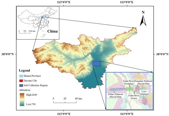
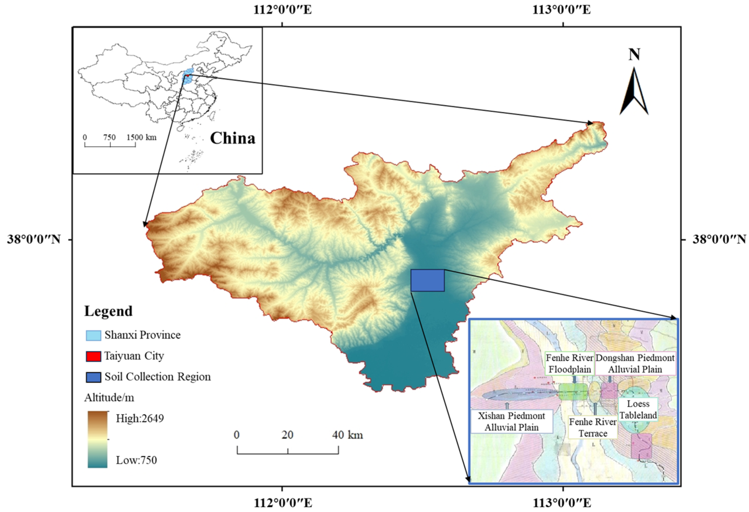
This study is based on the Taiyuan Metro Line 1 project. Undisturbed soil samples were collected from deep excavation pits at five representative stations. As illustrated in Figure 1, the sampling sites are strategically distributed from west to east, traversing five distinct geomorphic units: the Xishan piedmont alluvial plain, the Fenhe River floodplain, the Fenhe River terrace, the Dongshan piedmont alluvial plain, and the Loess tableland.

Figure 1. Location of the study area and distribution of sampling sites across different geomorphic units.

Collected samples were preliminarily classified based on physical indices, including color, particle size distribution, mineral composition, and natural water content. For brevity and clarity, the silty clay sample CL-XY-1 is selected as a representative case study to detail the calibration procedure for HSS model parameters; the determination process for other samples follows an identical protocol. In situ investigation indicates that the CL-XY-1 sample was retrieved from a depth of approximately 14.0 m. The soil is grayish-black, exhibits plasticity, and features a smooth cut surface with a homogeneous texture and significant organic content. Its primary physical properties are summarized in Table 3.

Table 3. Physical properties of silty clay CL-XY-1.

${\mathit{\gamma }}_{\mathit{s}\mathit{a}\mathit{t}}$	$\mathit{\gamma }$	${\mathit{e}}_0$	${\mathit{K}}_{\mathit{v}}$	$\mathit{\omega }$	${\mathit{I}}_{\mathit{P}}$	${\mathit{I}}_{\mathit{L}}$
/kN·m−3	/kN·m−3	/−	/cm·s−1	/%	/−	/−
19.4	15.2	0.778	5.4 × 10−6	27.3	10.8	0.94

Notes: ${\gamma }_{sat}$—saturation unit weight, $\gamma$—natural unit weight, $e_0$—initial void ratio, $K_v$—permeability coefficient, $\omega$—water content, $I_P$—plasticity index, $I_L$—liquidity index.

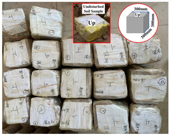
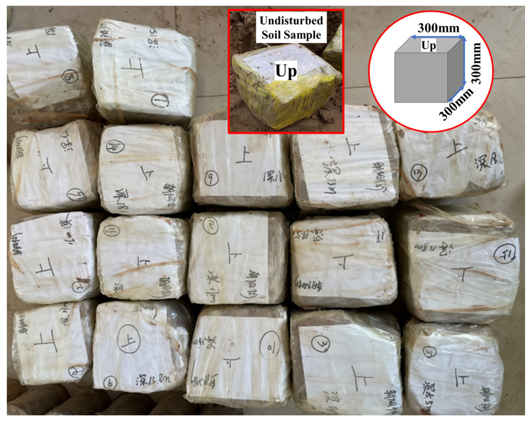
To ensure specimen representativeness and minimize disturbance, manual block sampling was employed at the excavation face. Undisturbed soil blocks were trimmed to dimensions of 300 mm × 300 mm × 300 mm (Figure 2). Immediately upon extraction, samples were oriented, sealed with multiple layers of plastic wrap and transparent tape to preserve natural moisture content. To minimize mechanical disturbance and prevent structural alteration during transportation, the specimens were placed in rigid containers with cushioning materials and transported to the laboratory on the same day. All samples were stored in a temperature-controlled environment, and laboratory tests were conducted within 7 to 10 days after sampling to ensure minimal changes in soil properties.

Figure 2. Preparation of undisturbed soil samples collected on site.

In total, the study acquired 8 silt samples, 7 silty clay samples, and 2 fine sand samples. Detailed numbering and sampling location information are provided in Table 4.

Table 4. Soil sample IDs and sampling locations.

Geomorphic Unit	Station	Depth/m	Soil Type	Sample ID
Xishan Piedmont Alluvial Plain	Xiayuan Station	−14.0	Silty clay	CL-XY-1
		−22.5	Silt	ML-XY-1
		−26.5	Silty clay	CL-XY-2
Fenhe River Floodplain	Yingzeqiaoxi Station	−12.5	Silt	ML-YZ-1
		−19.5	Silty clay	CL-YZ-1
		−21.0	Silty clay	CL-YZ-2
Fenhe River Terrace	Liuxiangnankou Station	−10.0	Silty sand	SM-LN-1
		−10.5	Silt	ML-LN-1
		−18.0	Silt	ML-LN-2
		−21.5	Silty clay	CL-LN-1
Dongshan Piedmont Alluvial Plain	Wusu Airport Station	−8.5	Silty sand	SM-JC-1
		−9.0	Silt	ML-JC-1
		−14.0	Silty clay	CL-JC-1
		−17.5	Silt	ML-JC-2
Loess Tableland	Chaoyangjie Station	−11.5	Silt	ML-CY-1
		−14.0	Silt	ML-CY-2
		−23.0	Silty clay	CL-CY-1

3.2. Experimental Design

To comprehensively quantify the input parameters required for the HSS model, a systematic laboratory testing program was conducted on the collected undisturbed soil samples. The program primarily comprises Standard Consolidation (SC), Consolidated Undrained (CU) triaxial, and Resonant Column (RC) tests. To ensure consistency in data processing, compressive stresses and strains are defined as positive throughout this study.

3.2.1. Standard Consolidation Test

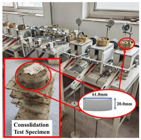
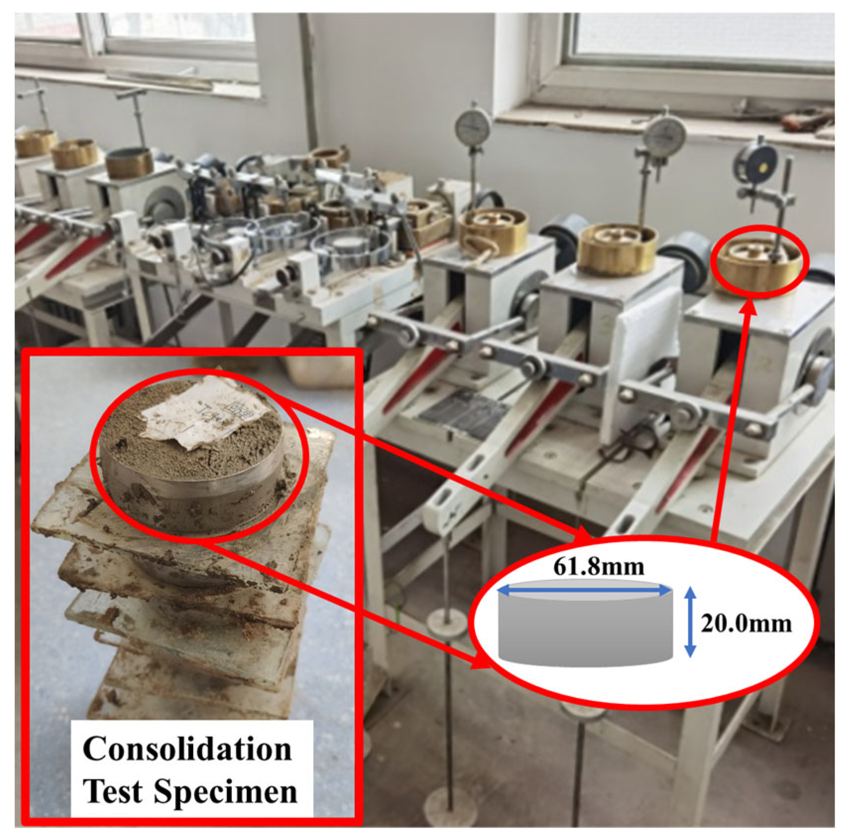
Standard Consolidation (SC) tests were performed using a high-pressure oedometer apparatus in accordance with ASTM D2435/D2435M [35]. The primary objective of the SC test is to induce one-dimensional consolidation by applying incremental vertical loads to a specimen confined in a rigid ring.

To accurately determine the reference unloading-reloading stiffness ($E_{ur}^{ref}$) for the HSS model, the loading sequence was modified from the conventional incremental loading method to include an unloading-reloading cycle. This cycle is essential for capturing the soil’s elastic rebounding behavior, which defines the HSS unloading-reloading parameters. The specific loading sequence was designed as follows: 25, 50, 100, 200 (unloading point), 100, 50, 25 (reloading point), 50, 100, 200, 400, 800, and 1600 kPa. The unloading point of 200 kPa was chosen because it corresponds to the typical average effective overburden stress level of the soil strata at the project site, ensuring the modulus is measured under representative stress conditions.

Following the incremental loading procedure, each load increment was maintained for 24 h, with the termination criterion that vertical deformation in the final hour be less than 0.01 mm to ensure the completion of primary consolidation. Vertical settlement was recorded in real-time throughout the process.

Cylindrical specimens were carefully trimmed to a diameter of 61.8 mm and a height of 20.0 mm. Great care was taken during the trimming process to minimize disturbance to the soil skeleton. The consolidation apparatus and prepared specimens are illustrated in Figure 3.

Figure 3. Consolidation test apparatus and prepared soil specimens.

3.2.2. Triaxial Consolidated Undrained Test

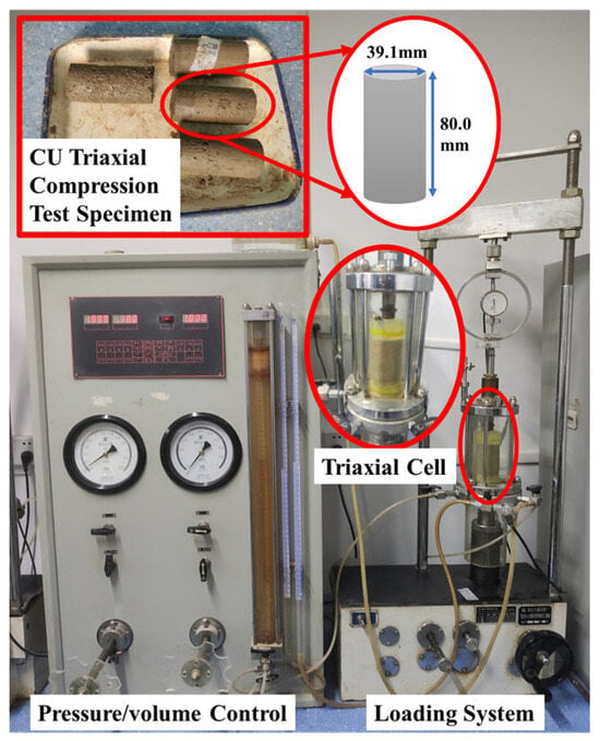
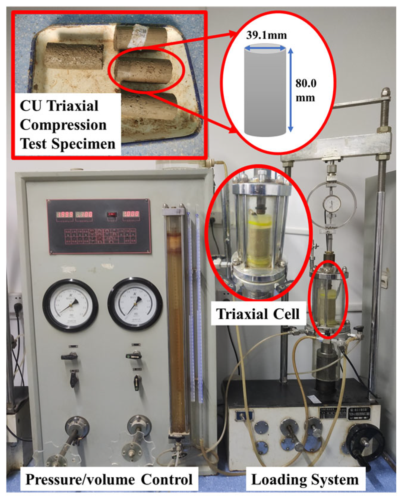
Triaxial Consolidated Undrained (CU) compression tests were conducted in accordance with ASTM D4767 [36]. For each soil sample, three standard cylindrical specimens (diameter 39.1 mm, height 80.0 mm) were prepared and sheared under effective confining pressures of 100, 200, and 400 kPa, respectively.

The testing protocol comprised three distinct phases:

• Saturation Phase: A dual-stage saturation method combining vacuum and back-pressure saturation was employed. First, specimens were placed in a vacuum cylinder and evacuated for over 12 h to achieve initial saturation. Subsequently, the specimens were mounted in the triaxial cell. To monitor the saturation development, Skempton’s pore pressure coefficient B was measured repeatedly after each incremental increase in cell pressure and back pressure. The back pressure was increased in stages while maintaining a constant effective stress differential of 50 kPa until the B-coefficient was verified to reach 0.95, ensuring full saturation before proceeding to consolidation.
• Consolidation Phase: Saturated specimens underwent isotropic consolidation under the target confining pressures. The primary consolidation was deemed complete when the volumetric change was less than 0.1 cm³ over a consecutive period of 1 to 2 h.
• Shearing Phase: Upon completion of consolidation, the drainage valve was closed to conduct undrained shearing under strain-controlled conditions. In accordance with ASTM D4767, a shear rate of 0.04 mm/min was selected based on the drainage characteristics of the specimens to ensure the equalization of pore water pressure throughout the shearing process. Axial load, deformation, and pore water pressure were recorded in real-time via an automated data acquisition system. The test was terminated when the deviatoric stress peaked or when the axial strain reached 15% (in cases with no distinct peak).

The triaxial testing apparatus and representative specimens are shown in Figure 4.

Figure 4. Triaxial test apparatus and prepared soil specimens.

3.2.3. Resonant Column Test

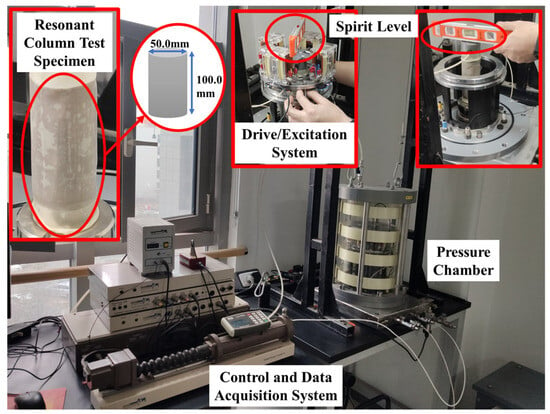
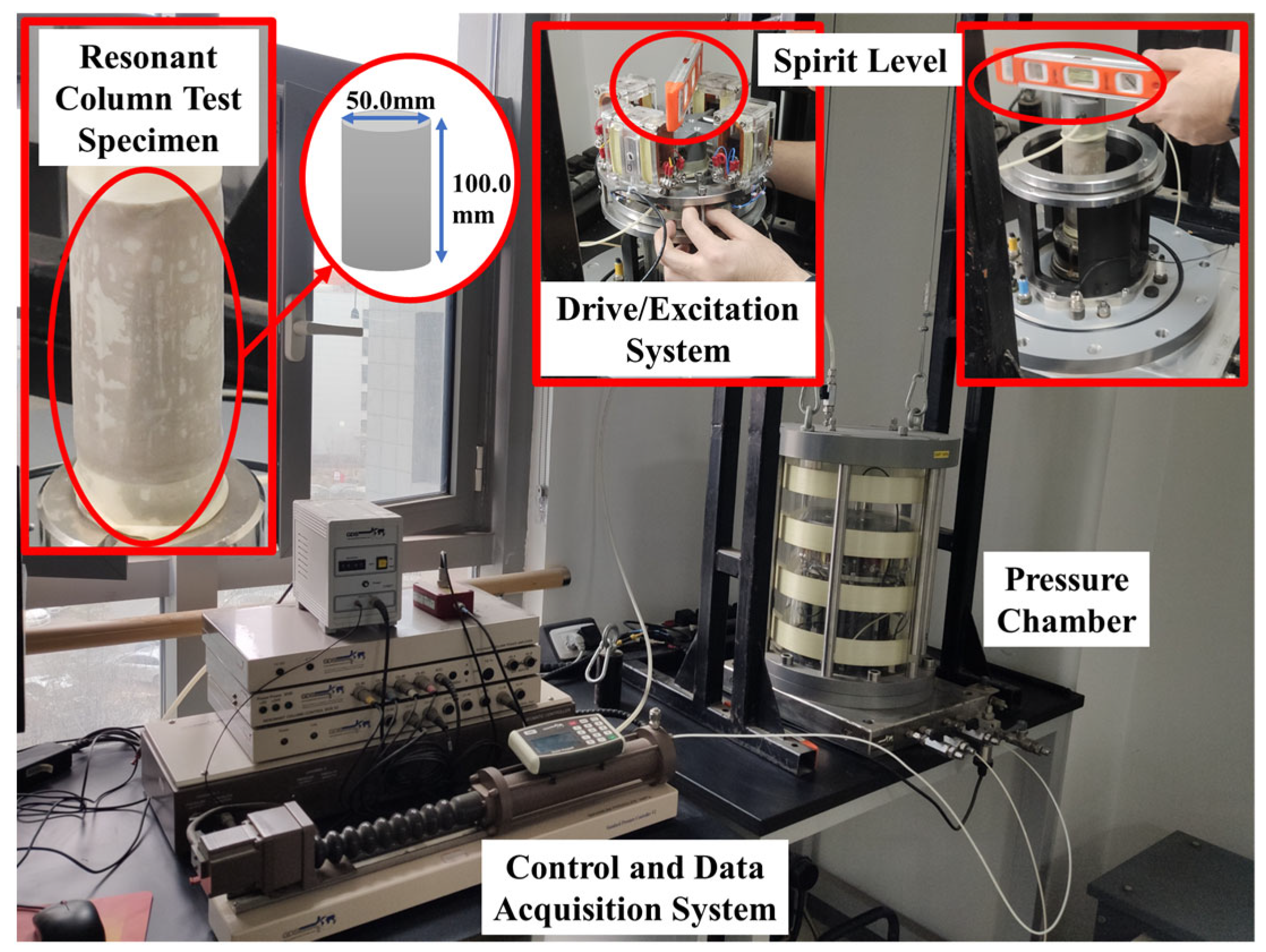
To accurately determine the reference small-strain shear modulus ($G_0^{ref}$) and its degradation characteristics, Resonant Column (RC) tests were conducted in accordance with ASTM D4015 [37]. The testing utilized a Stokoe-type Resonant Column Apparatus (RCA) manufactured by GDS Instruments, UK, capable of applying a maximum confining pressure of 1000 kPa. Cylindrical specimens were prepared with a diameter of 50.0 mm and a height of 100.0 mm.

The experimental procedure comprised four key stages:

• Specimen Installation and Saturation: The test adopted a “fixed-free” boundary condition configuration. Specimens were first subjected to vacuum saturation and then mounted between the drive plate and the fixed pedestal. A precision spirit level and alignment device were employed to ensure strict verticality and centrality of the specimen (as highlighted in Figure 5). Following installation, back-pressure saturation was applied until Skempton’s pore pressure coefficient B reached ≥0.95.
• Consolidation Phase: Saturated specimens underwent isotropic consolidation under an effective confining pressure of 100 kPa. Drainage volume was monitored in real-time; the primary consolidation was considered complete when the volumetric change was less than 200 mm² (approximately 0.1% of the specimen volume) over a consecutive 1 h period.
• Excitation and Measurement: An electromagnetic drive system applied low-amplitude torsional vibrations to the specimen top. A frequency sweep was performed within a range of 10 to 250 Hz, and the vibration amplitude was incrementally adjusted to capture the soil response across a shear strain range of 10⁻⁶ to 10⁻⁴. A frequency sweep mode was employed via a closed-loop control system to identify the first-mode resonant frequency (f_n). The resonance state was identified as the frequency at which the dynamic response reached its maximum amplitude, corresponding to a 90° phase lag between the applied torque and the resulting angular displacement. Based on elastic wave propagation theory, the dynamic shear modulus (G) and damping ratio (D) were calculated across a range of shear strain amplitudes (γ).
• Data Acquisition and Correction: Torque, angular displacement, and frequency signals were recorded by the GDS data acquisition system. Prior to the experimental program, the apparatus underwent rigorous calibration using standard aluminum specimens of known properties to determine the rotational inertia of the drive system and ensure measurement precision. To eliminate the influence of equipment rigidity on the results, all raw data underwent system compliance correction, ensuring the accuracy of measurements for high-stiffness soil specimens.

Figure 5. Resonant column test apparatus and prepared soil specimens.

The resonant column testing apparatus and specimen preparation details are illustrated in Figure 5.

3.3. Calculation of Key Parameters

3.3.1. Determination of Effective Strength Parameters

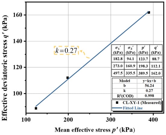
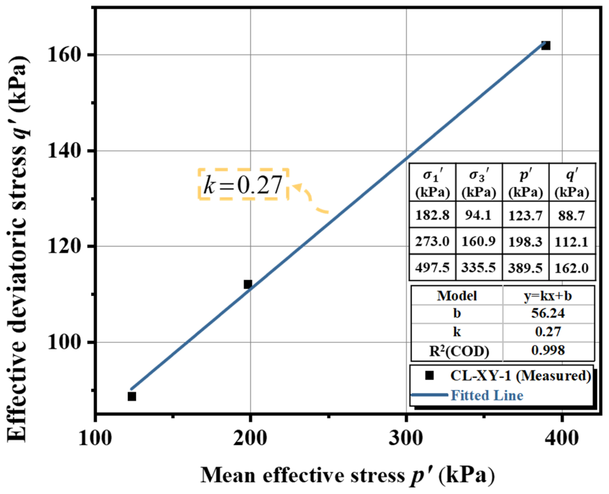
Based on the results of the CU tests, the effective strength parameters—effective cohesion c′ and effective friction angle φ′—were determined using the p′-q′ stress path method combined with the Mohr–Coulomb failure criterion.

In the principal stress space, the Mohr–Coulomb failure criterion is expressed as:

$$0.5\left({\sigma }_1^{\prime }-{\sigma }_3^{\prime }\right)-0.5\left({\sigma }_1^{\prime }+{\sigma }_3^{\prime }\right)\times \mathit{sin}{\phi }^{\prime }-c^{\prime }\mathit{cos}{\phi }^{\prime }=0$$

(1)

Introducing the mean effective stress p′ = (σ₁′ + 2σ₃′)/3 and the deviatoric stress q′ = σ₁′ − σ₃′, Equation (1) can be rewritten as a linear relation in the p′-q′ plane:

$$q^{\prime }=M{p}^{\prime }+N={\displaystyle \frac{6\mathit{sin}{\phi }^{\prime }}{3-\mathit{sin}{\phi }^{\prime }}}{p}^{\prime }+{\displaystyle \frac{6c^{\prime }\mathit{cos}{\phi }^{\prime }}{3-\mathit{sin}{\phi }^{\prime }}}$$

(2)

Figure 6 presents the failure stress states of sample CL-XY-1 under different confining pressures and the corresponding linear regression results. The experimental data show strong linearity (R² > 0.99), yielding the fitted relationship: q′ = 0.27p′ + 56.24.

Figure 6. Determination of effective strength parameters for sample CL-XY-1.

By equating the regression parameters with the theoretical expressions in Equation (2), the effective strength parameters of sample CL-XY-1 were obtained as: c′ = 27.2 kPa, φ′ = 7.4°.

3.3.2. Reference Oedometer Stiffness

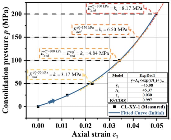
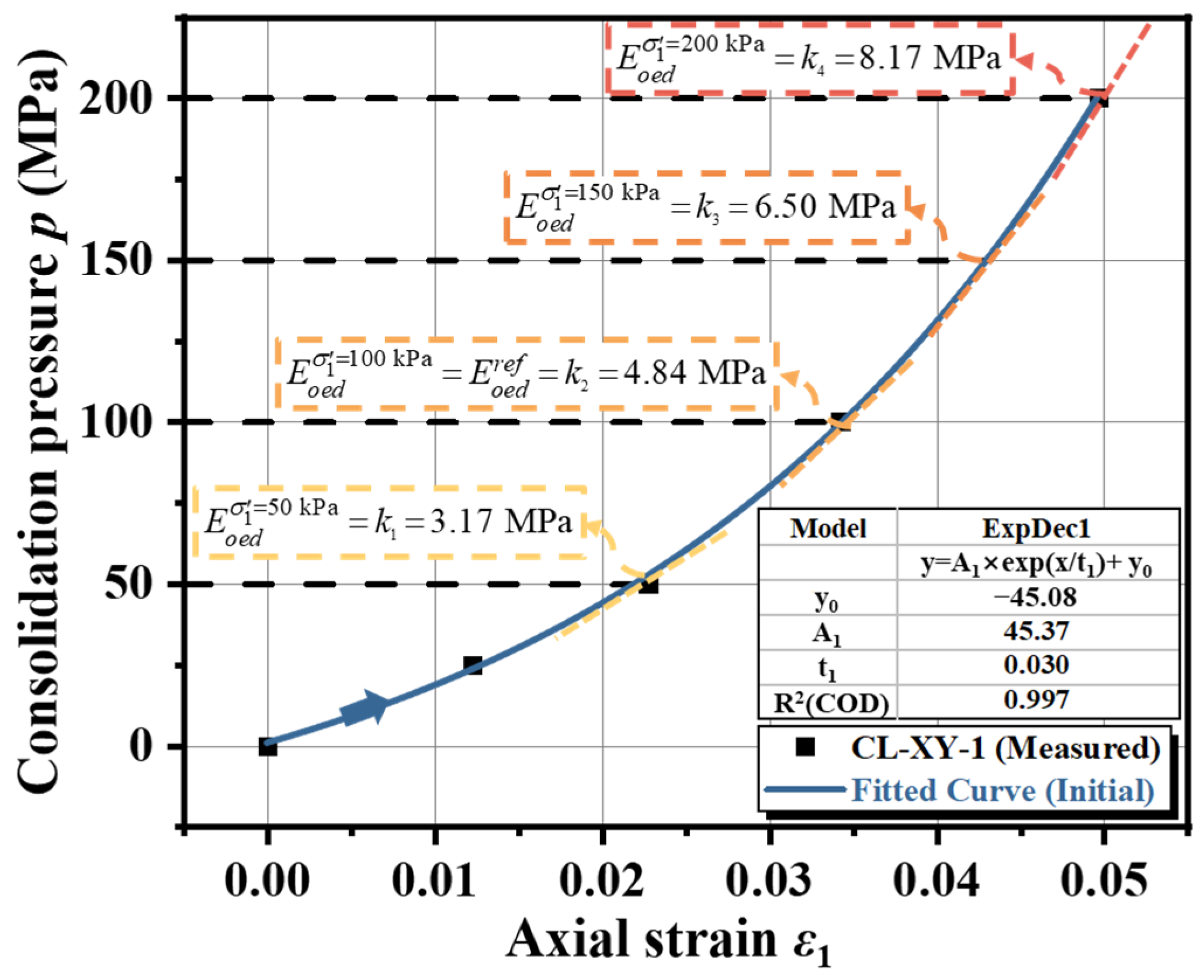
Figure 7 presents the standard consolidation test results for the representative sample CL-XY-1 during the initial loading stage (0–200 kPa). The scatter plot of vertical load p versus axial strain ε1 reveals a distinct non-linear relationship. As the load increases, the slope of the curve gradually steepens, indicating that the soil stiffness increases with stress level (i.e., strain hardening behavior).

Figure 7. Determination of reference oedometer stiffness.

To accurately quantify this non-linear response, an exponential growth model, y = y₀ + Ae^(x/t), was employed to perform a non-linear regression analysis on the experimental data, where A, t, and y₀ are fitting parameters. The regression yields the equation p = −45.08 + 45.37e^ε1/0.030, with a coefficient of determination R² exceeding 0.99, demonstrating that this model provides an excellent description of the soil’s compression behavior under confined conditions.

According to the HSS model definition, the reference oedometer stiffness $E_{oed}^{ref}$ corresponds to the tangent stiffness of the p-ε₁ curve at the reference pressure $P^{ref}=100 \mathrm{k}\mathrm{P}\mathrm{a}$. By differentiating the fitted equation with respect to strain and substituting the strain value corresponding to p = 100 kPa, the tangent stiffness for sample CL-XY-1 is calculated as:

$$E_{oed}^{ref}={\left.{\displaystyle \frac{dp}{d{\epsilon }_1}}\right|}_{p=100\mathrm{k}\mathrm{P}\mathrm{a}}=4.84 \mathrm{M}\mathrm{P}\mathrm{a}$$

This calculated value is consistent with the tangent slope marked as k₂ in Figure 7, verifying the reliability of the fitted model parameters.

3.3.3. Stress Dependency Exponent

In the theoretical framework of the HSS model, the complete expression for the oedometer stiffness $E_{oed}$, incorporating strength parameters (effective cohesion c’ and effective friction angle φ’), is given by Equation (3) [14]:

$$E_{oed}=E_{oed}^{ref}{\left({\displaystyle \frac{{\sigma }_1^{\prime }\mathit{sin}{\phi }^{\prime }+c^{\prime }\mathit{cos}{\phi }^{\prime }}{p^{ref}\mathit{sin}{\phi }^{\prime }+c^{\prime }\mathit{cos}{\phi }^{\prime }}}\right)}^m$$

(3)

Under standard one-dimensional compression conditions (K₀-consolidation), the ratio between the deviatoric stress q and the mean effective stress p’ remains constant, meaning the influence of the failure envelope on stiffness becomes constant. Consequently, the non-linear stiffness hardening is primarily governed by the mean effective stress. Equation (3) can thus be simplified to a power-law form dependent solely on stress level, as shown in Equation (4):

$$E_{oed}=E_{oed}^{ref}{\left({\sigma }_1^{\prime }/p^{ref}\right)}^m$$

(4)

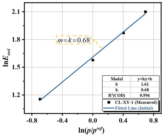
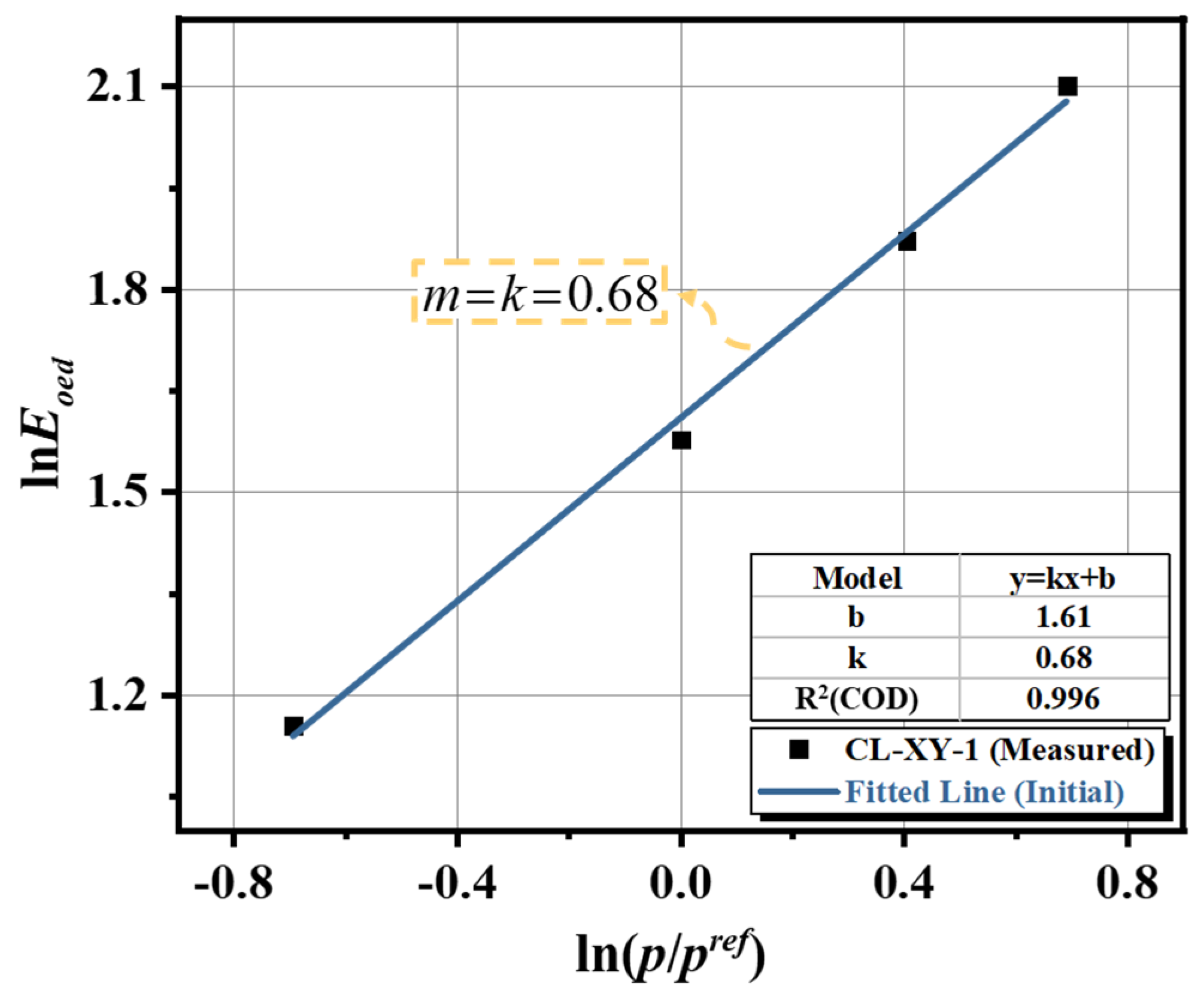
where σ₁′ is the vertical effective stress, which equals the consolidation pressure p in standard oedometer tests. To determine the exponent m, a natural logarithm transformation is applied to both sides of Equation (4) to linearize the relationship:

$$\mathit{ln}{E}_{oed}=\mathit{ln}{E}_{oed}^{ref}+m\mathit{ln}\left(p/p^{ref}\right)$$

(5)

Based on the stiffness function derived in Section 3.3.2 (the derivative of the p-ε₁ curve), the tangent stiffness moduli $E_{oed}$ at consolidation pressures of 50, 100, 150, and 200 kPa were calculated as 3.17 MPa, 4.84 MPa, 6.50 MPa, and 8.17 MPa, respectively.

Figure 8 illustrates the scatter plot of $\ln E_{oed}$-$\ln \left(p/p^{ref}\right)$ for sample CL-XY-1, along with the linear regression results. The data points exhibit a strong linear correlation in the double-logarithmic coordinate system R² > 0.99. The fitted linear equation is y = 0.68x + 1.61. Since the slope of this line represents the stress dependency exponent, the value is determined as m = 0.68.

Figure 8. Determination of stress dependency exponent.

It should be noted that while different stiffness moduli (e.g., $E_{oed}$, $E_{50}$, $E_{ur}$, $G_0$) in natural soils may exhibit slight variations in their stress dependency, the HSS model adopts a unified m value throughout its constitutive framework. This simplification ensures mathematical elegance, facilitates parameter calibration, and guarantees numerical convergence and stability. Engineering practice has demonstrated that using a unified m value effectively avoids numerical instability caused by over-parameterization while maintaining sufficient accuracy for engineering applications.

3.3.4. Reference Unloading/Reloading Stiffness

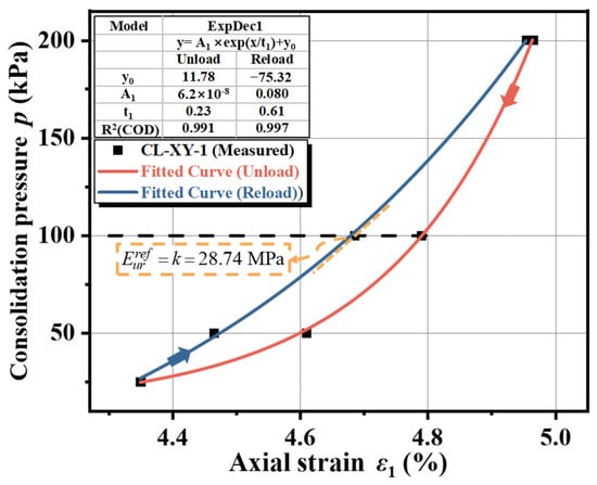
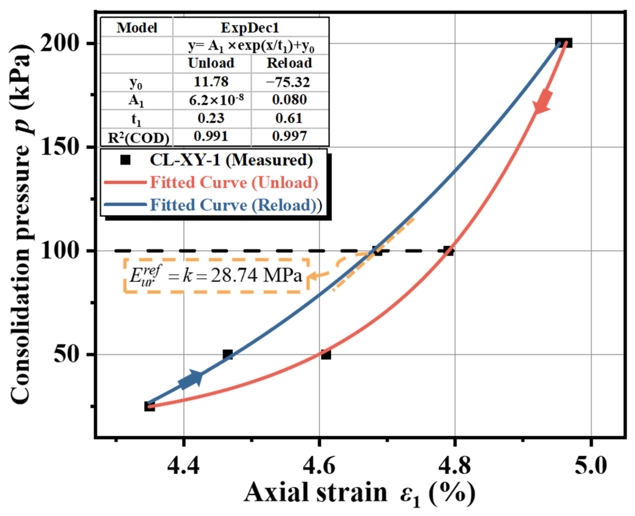
The HSS model assumes elastic behavior during unloading and reloading stress paths. While triaxial unloading tests are the ideal source for this parameter, deriving $E_{ur}^{ref}$ from the “unloading-reloading” hysteresis loop in SC tests is a widely accepted and effective alternative in engineering practice [38]. During this phase, the soil undergoes rebound and recompression, which can be approximated as elastic deformation.

Following the methodology recommended by PLAXIS, this study applies the same mathematical framework used in Section 3.3.2 to the reloading branch of the hysteresis loop.

According to the definition, the reference unloading-reloading stiffness $E_{ur}^{ref}$ is the tangent stiffness of the reloading curve at the reference pressure $P^{ref}=100 \mathrm{k}\mathrm{P}\mathrm{a}$. Differentiating the fitted equation and substituting the corresponding strain yields a value of $E_{ur}^{ref}=28.74$ MPa for sample CL-XY-1. This calculated stiffness is visually consistent with the tangent slope marked in Figure 9, verifying the accuracy of the parameter extraction.

Figure 9. Determination of reference unloading-reloading stiffness.

3.3.5. Reference Secant Stiffness

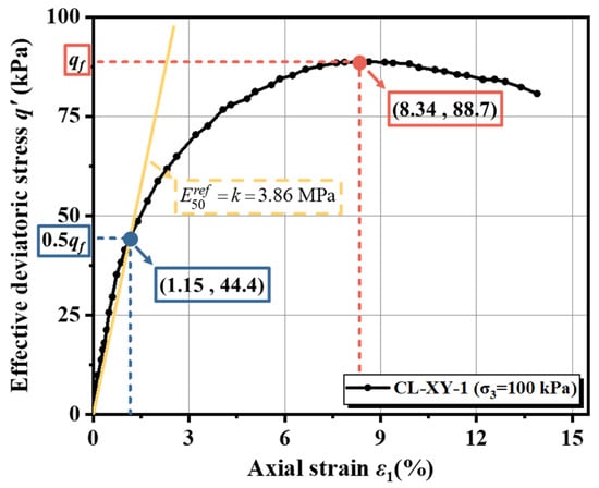
The reference secant stiffness $E_{50}^{ref}$ is the primary parameter governing plastic shear deformation within the HSS model framework. It is defined as the secant stiffness corresponding to 50% of the ultimate deviatoric stress q′ on the deviatoric stress-axial strain (q′-ε₁) curve, obtained from standard triaxial compression tests at a reference confining pressure of $P^{ref}=100 \mathrm{k}\mathrm{P}\mathrm{a}$.

The ultimate deviatoric stress $q_f$ is defined as the asymptotic peak stress. In the absence of a distinct peak, the stress corresponding to 15% axial strain is adopted as the failure value.

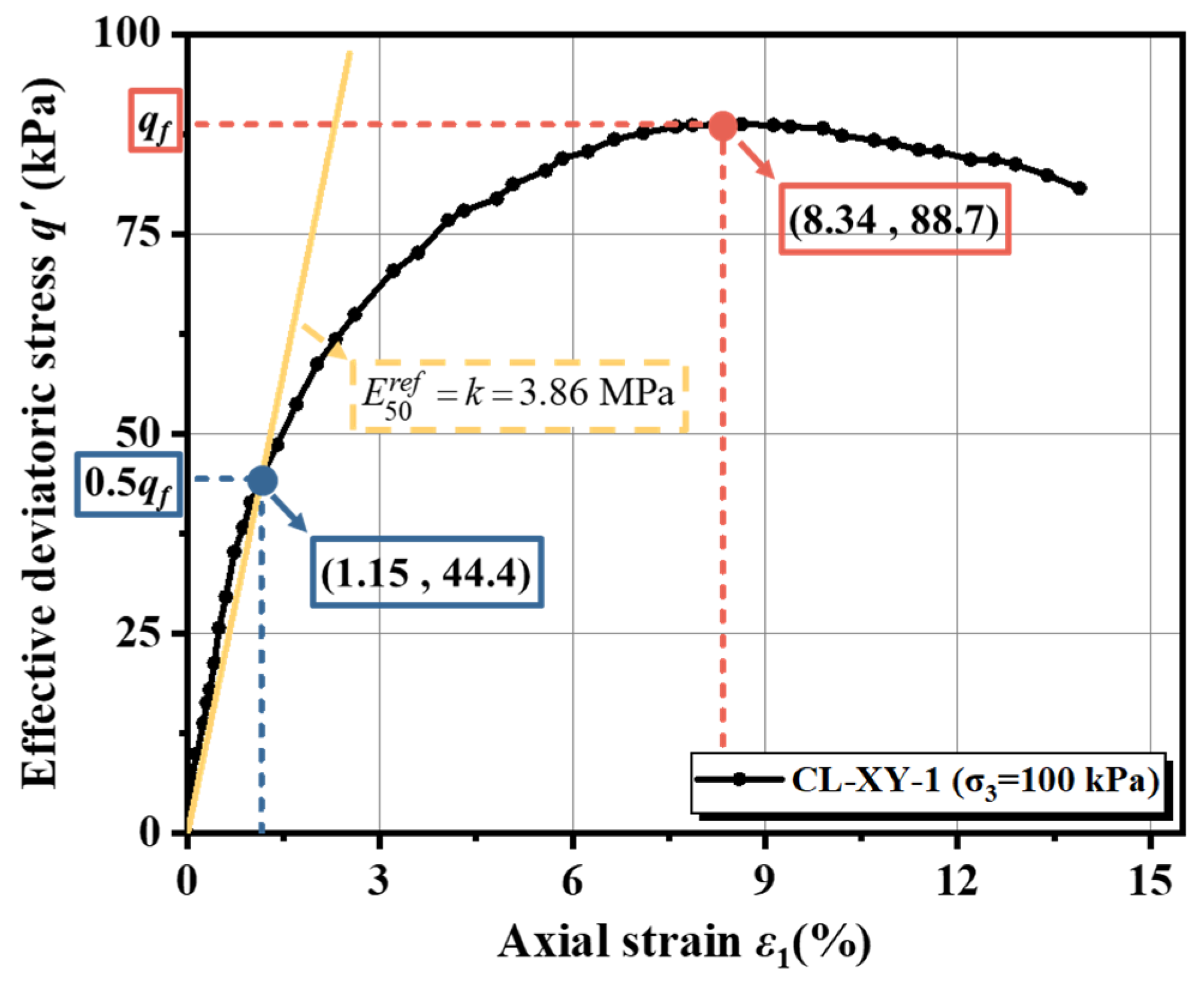
Figure 10 presents the deviatoric stress versus axial strain (q′-ε₁) curve for sample CL-XY-1 under the reference confining pressure of 100 kPa. Following the definition above, a secant line was drawn connecting the origin to the stress point corresponding to 0.5 $q_f$. The slope of this line represents the reference secant stiffness. For sample CL-XY-1, the calculated value is $E_{50}^{ref}=3.86$ MPa.

Figure 10. Determination of reference secant stiffness.

3.3.6. Reference Small-Strain Shear Modulus

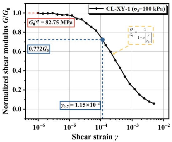
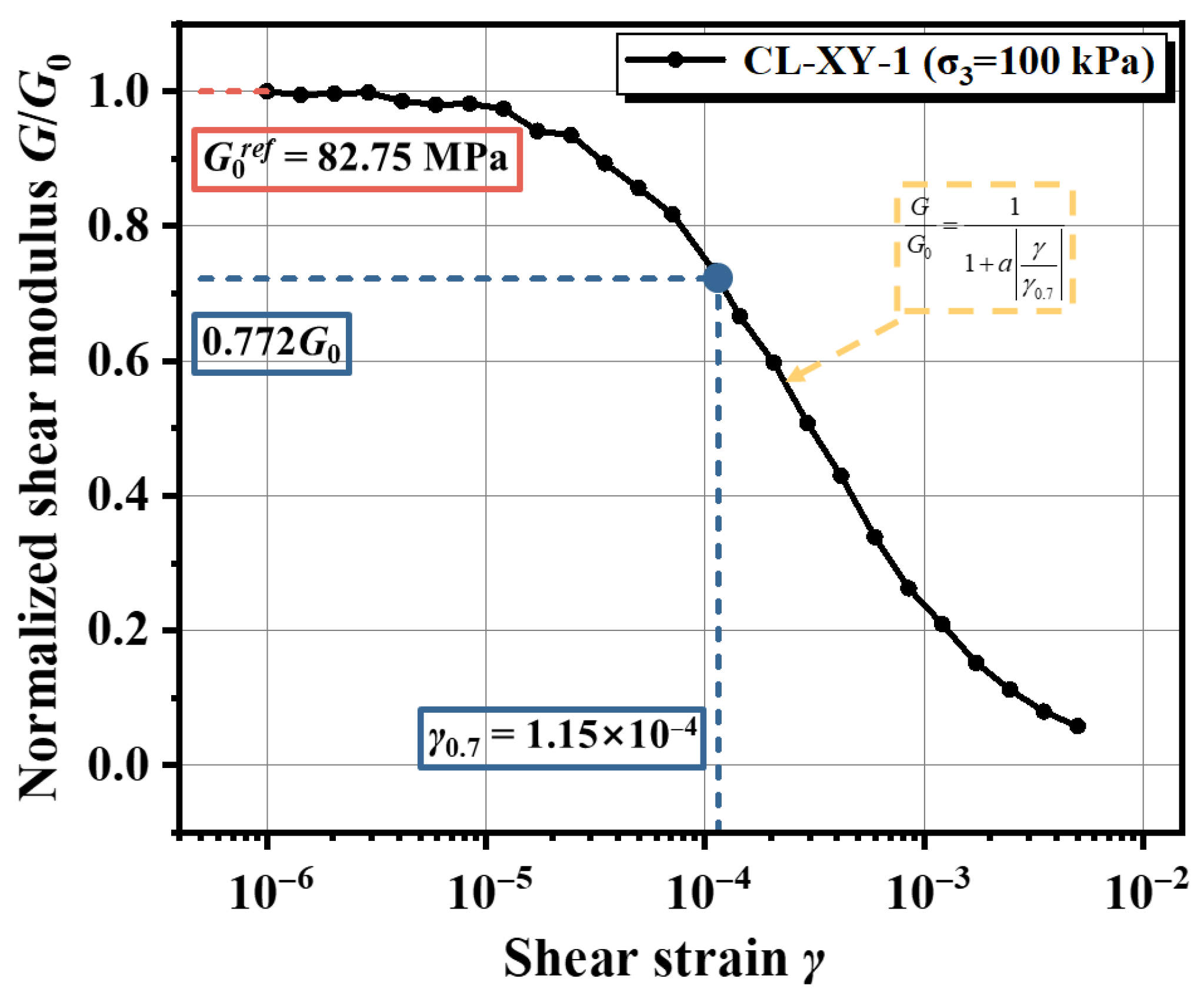
The non-linear decay characteristics of the dynamic shear modulus $G$ with increasing shear strain $\gamma$ are typically described using the hyperbolic model proposed by Hardin et al. [14]. Building upon this framework, Santos [39] introduced a threshold shear strain parameter ${\gamma }_{0.7}$, defined as the strain amplitude at which the secant shear modulus degrades to approximately 72.2% of its initial small-strain value, to normalize the decay curve. The modified normalized small-strain stiffness decay model is expressed as:

$${\displaystyle \frac{G}{G_0}}={\displaystyle \frac{1}{1+a\left|\frac{\gamma }{{\gamma }_{0.7}}\right|}}$$

(6)

In Equation (6), $a$ is a curve-fitting parameter set to 0.385. $G_0$ represents the initial dynamic shear modulus as shear strain approaches zero, which is equivalent to the maximum shear modulus $G_{max}$. Within the definition of the HSS model, the initial shear modulus measured under the reference confining pressure $P^{ref}={\sigma }_3=100 \mathrm{k}\mathrm{P}\mathrm{a}$ is designated as the reference small-strain shear modulus $G_0^{ref}$.

Figure 11 illustrates the semi-logarithmic relationship between the normalized dynamic shear modulus and shear strain ($G/G_0$-$\gamma$) for sample CL-XY-1 under a confining pressure of 100 kPa. The experimental data were fitted using Equation (6), demonstrating a strong correlation. The analysis yields a reference small-strain shear modulus of $G_0^{ref}=82.75$ MPa and a corresponding threshold shear strain of ${\gamma }_{0.7}=1.15\times {10}^{-4}$.

Figure 11. Determination of reference small-strain shear modulus parameters.

To further assess the applicability of the measured modulus reduction behavior, the obtained G/G₀–γ curves were qualitatively compared with widely accepted empirical relationships, including those proposed by Vucetic and Dobry (1991) [40] and Darendeli (2001) [41]. Under comparable confining pressure conditions, the degradation trends of the tested silty and clayey soils fall within the typical empirical envelopes reported for soils of similar plasticity. The threshold shear strain values obtained in this study indicate moderate stiffness degradation characteristics, consistent with the transitional microstructure of loess-derived deposits. While detailed quantitative plotting against multiple empirical curves for each soil category is beyond the scope of the present work, such systematic comparison would provide further validation of the regional stiffness characterization.

3.4. Summary of Key Parameters

By integrating the experimental data from the SC, CU, and RC tests with the theoretical framework of the HSS model, the key constitutive parameters for 17 undisturbed soil samples—comprising typical silt (ML), silty clay (CL), and silty sand (SM) from the Taiyuan region—were systematically calibrated.

The calibrated physico-mechanical parameters are summarized in Table 5. This comprehensive dataset encompasses the effective strength parameters (c′, φ′) governing failure behavior, the stress dependency exponent (m), and the critical stiffness parameters ($E_{oed}^{ref}$, $E_{50}^{ref}$, $E_{ur}^{ref}$, $G_0^{ref}$) characterizing the deformation response across the entire strain spectrum—from small-strain elasticity to large-strain plasticity.

Table 5. Summary of calibrated HSS model parameters for all soil samples.

Sample ID	c′	φ′	${\mathit{E}}_{\mathit{o}\mathit{e}\mathit{d}}^{\mathit{r}\mathit{e}\mathit{f}}$	${\mathit{E}}_{50}^{\mathit{r}\mathit{e}\mathit{f}}$	${\mathit{E}}_{\mathit{u}\mathit{r}}^{\mathit{r}\mathit{e}\mathit{f}}$	${\mathit{G}}_0^{\mathit{r}\mathit{e}\mathit{f}}$	${\mathit{\gamma }}_{0.7}$	m
	/kPa	/°	/MPa	/MPa	/MPa	/MPa	$/\times {10}^{-4}$	/−
ML-XY-1	11.1	16.0	11.76	12.53	45.94	96.84	1.58	0.50
ML-YZ-1	11.4	26.9	6.55	5.11	21.56	90.10	1.41	0.56
ML-LN-1	17.6	28.8	8.44	9.95	38.70	88.13	1.38	0.76
ML-LN-2	18.2	32.7	11.67	12.80	57.64	104.23	1.78	0.56
ML-JC-1	20.3	31.3	8.16	10.75	31.92	98.57	1.22	0.60
ML-JC-2	25.3	29.7	9.69	10.89	39.41	91.85	1.51	0.66
ML-CY-1	16.8	11.1	6.97	5.60	36.77	95.71	1.80	0.78
ML-CY-2	18.0	21.4	8.39	9.04	41.35	91.85	1.43	0.66
CL-XY-1	27.2	7.4	4.84	3.86	28.74	82.75	1.15	0.68
CL-XY-2	37.0	3.4	5.33	4.22	21.94	84.31	0.96	0.61
CL-YZ-1	39.0	10.4	10.48	12.05	44.07	95.85	1.02	0.71
CL-YZ-2	44.1	12.3	3.58	3.20	23.78	83.20	1.22	0.65
CL-LN-1	30.9	23.0	8.15	8.47	32.51	88.79	0.95	0.69
CL-JC-1	39.3	27.5	7.52	6.20	22.19	80.29	0.91	0.81
CL-CY-1	55.5	13.7	4.63	5.13	20.79	78.64	1.12	0.61
SM-LN-1	7.0	32.4	17.53	20.35	78.57	113.66	2.78	0.57
SM-JC-1	7.3	37.7	19.03	24.47	73.08	121.43	2.49	0.55

As evidenced in Table 5, the parameters exhibit significant variability across different soil lithologies. This heterogeneity underscores the necessity of carrying out site-specific parameter calibration rather than relying on generic values. Furthermore, this high-quality dataset provides a robust foundation for the subsequent development of regional empirical correlations for stiffness parameters and for the execution of accurate numerical simulations of deep excavations in the Taiyuan area.

4. Statistical Analysis of Key Stiffness Parameters

4.1. Correlations Between Stiffness Parameters

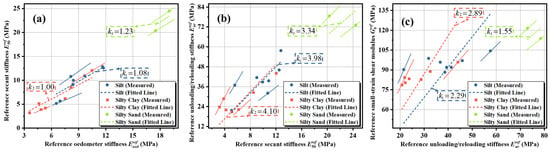
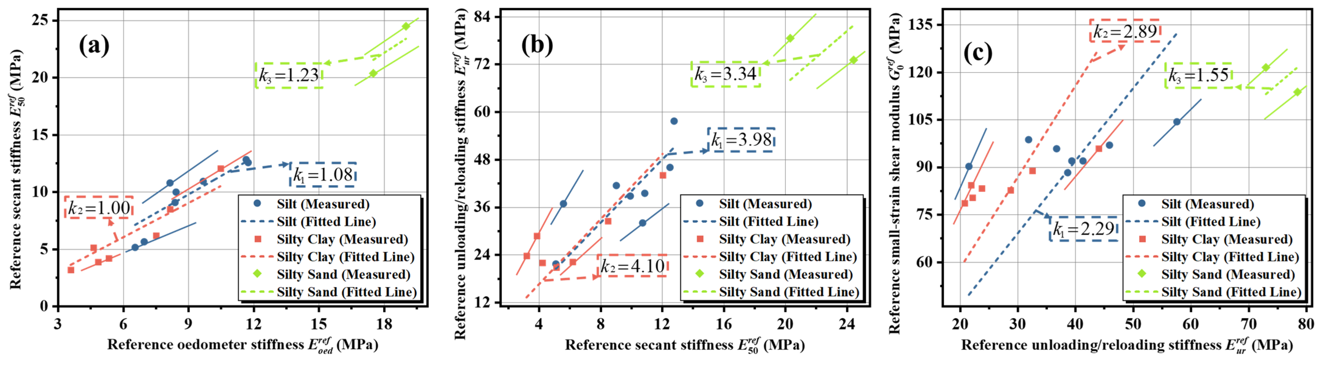
To elucidate the intrinsic interdependencies among the HSS model parameters for typical soil layers in the Taiyuan region, a systematic correlation analysis was conducted based on the results from the SC, CU, and RC tests. Using zero-intercept linear regression, quantitative relationships were established between $E_{50}^{ref}$ versus $E_{oed}^{ref}$, $E_{ur}^{ref}$ versus $E_{50}^{ref}$, and $G_0^{ref}$ versus $E_{ur}^{ref}$, as illustrated in Figure 12. The regression results indicate significant positive linear correlations among the various stiffness moduli, where the slope of the regression line represents the conversion coefficient between specific stiffness parameters under comparable lithological and stress conditions.

Figure 12. Correlations between stiffness parameters for typical soil layers in Taiyuan. (a) Relationship between reference secant stiffness and reference oedometer stiffness. (b) Relationship between reference unloading-reloading stiffness and reference secant stiffness. (c) Relationship between reference small-strain shear modulus and reference unloading-reloading stiffness. The dashed lines represent linear regressions through the origin, with the slope k indicating the stiffness ratio.

In this study, zero-intercept linear regression was utilized to derive simplified conversion coefficients for practical engineering use. The high correlation coefficients (R² > 0.9) observed across the datasets support the validity of the linear approach within the tested stress ranges, as the slope of the regression line represents a stable conversion coefficient between specific stiffness parameters.

Regarding the observed differences between soil layers, the Silt layer exhibited a relatively lower $G_0^{ref}$/$E_{ur}^{ref}$ ratio compared to Silty Clay. This phenomenon can be attributed to the fact that stiffness characteristics and stress sensitivity tend to intensify with increasing fines content. The Silty Clay in this region possesses a more distinct structural potential, leading to stiffness degradation characteristics that differ from those of the transitional Silt layer.

Based on the linear regression analysis, this study established the normalized stiffness parameter ratios ($E_{oed}^{ref}$:$E_{50}^{ref}$:$E_{ur}^{ref}$:$G_0^{ref}$) for representative soils in the Taiyuan area under reference stress states. Specifically:

Silt (ML): The stiffness ratio is 1.00:1.08:4.30:9.85.

Silty Clay (CL): Exhibits a relatively higher small-strain stiffness ratio, with a relationship of 1.00:1.00:4.10:11.85.

Silty Sand (SM): The ratio is determined as 1.00:1.23:4.11:6.37.

These empirical proportional relationships quantitatively describe the evolution of soil stiffness from the static large-strain regime to the dynamic small-strain regime.

It should be noted that the correlations for silty sand are derived from a more limited number of samples compared to silt and silty clay due to geological constraints. Although the regression shows high consistency, these specific ratios should be regarded as preliminary and indicative, and further validation with in situ tests is recommended.

More broadly, while the proposed stiffness ratios serve as regional reference values for soils with similar genesis and stress history, they demonstrate a systematic calibration approach. Therefore, these results should be adopted for other regions through site-specific testing rather than direct numerical transfer.

4.2. Regional Comparison of Stiffness Parameter Ratios

To further contextualize the stiffness ratios established for Taiyuan soils, a comparative analysis was conducted based on the regional data summarized in Table 2. The objective is to evaluate similarities and differences between the present results and previously reported HS/HSsmall parameter systems under various geological conditions.

• Comparison of $E_{50}^{ref}/$$E_{oed}^{ref}$

The ratio $E_{50}^{ref}$/$E_{oed}^{ref}$ for Taiyuan soils ranges from 1.00 to 1.23, indicating that the triaxial secant stiffness is comparable to or slightly greater than the oedometer stiffness.

This range is consistent with values reported for silty and clayey soils in Ningbo, Hangzhou, and London, where ratios generally vary between approximately 0.9 and 1.5. However, lower values have been reported in Nanjing silty clay (~0.53), reflecting more pronounced compression-dominated behavior in highly structured soft clays.

The relatively stable ratio observed in Taiyuan suggests balanced shear and compression stiffness development, likely associated with the transitional nature of loess-derived silty deposits.

• Comparison of $E_{ur}^{ref}/$$E_{50}^{ref}$

The unloading–reloading stiffness ratio in Taiyuan (4.10–4.30) falls within the lower-to-intermediate range of reported values. International data indicate a wide variation, from approximately 3.0 (Varberg and Lisbon clays) to over 14.0 (Nanjing silty clay).

Compared with highly overconsolidated marine clays, the moderate amplification observed in Taiyuan suggests a less pronounced stress-history effect. This difference may be attributed to lower plasticity indices, weaker cementation, and distinct depositional environments compared with coastal soft clays.

• Comparison of $G_0^{ref}/$$E_{ur}^{ref}$

The most significant regional variation is observed in the small-strain stiffness ratio. For Taiyuan soils, $G_0^{ref}$/$E_{ur}^{ref}$ ranges from 6.37 to 11.85.

These values are comparable to those reported for Hangzhou clay and Incheon sediment, but lower than the ratio reported for London Clay (~22.05), which is characterized by strong overconsolidation and pronounced bonding effects.

The moderate small-strain amplification in Taiyuan soils reflects their microstructural characteristics—primarily loess-derived silty deposits with limited cementation and moderate structural potential. Additionally, differences in laboratory testing conditions (e.g., confining pressure levels and resonant column procedures) may contribute to variability.

• Implications for Engineering Application

The stiffness ratios established in this study fall within the broader range reported in the previous literature but exhibit distinct regional characteristics. This confirms that regional calibration is essential for reliable HSS parameter selection.

The present study therefore contributes a localized parameter system for Taiyuan soils while maintaining consistency with the broader international database. The methodology adopted herein may also provide a reference framework for establishing stiffness parameter systems in other regions through systematic laboratory calibration and regression analysis.

4.3. Distribution Characteristics of Stress Dependency Exponent

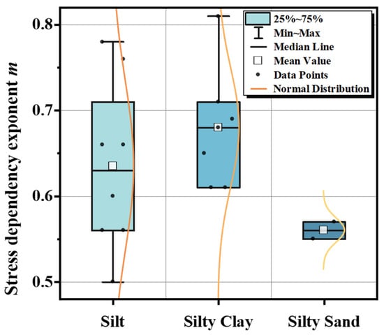
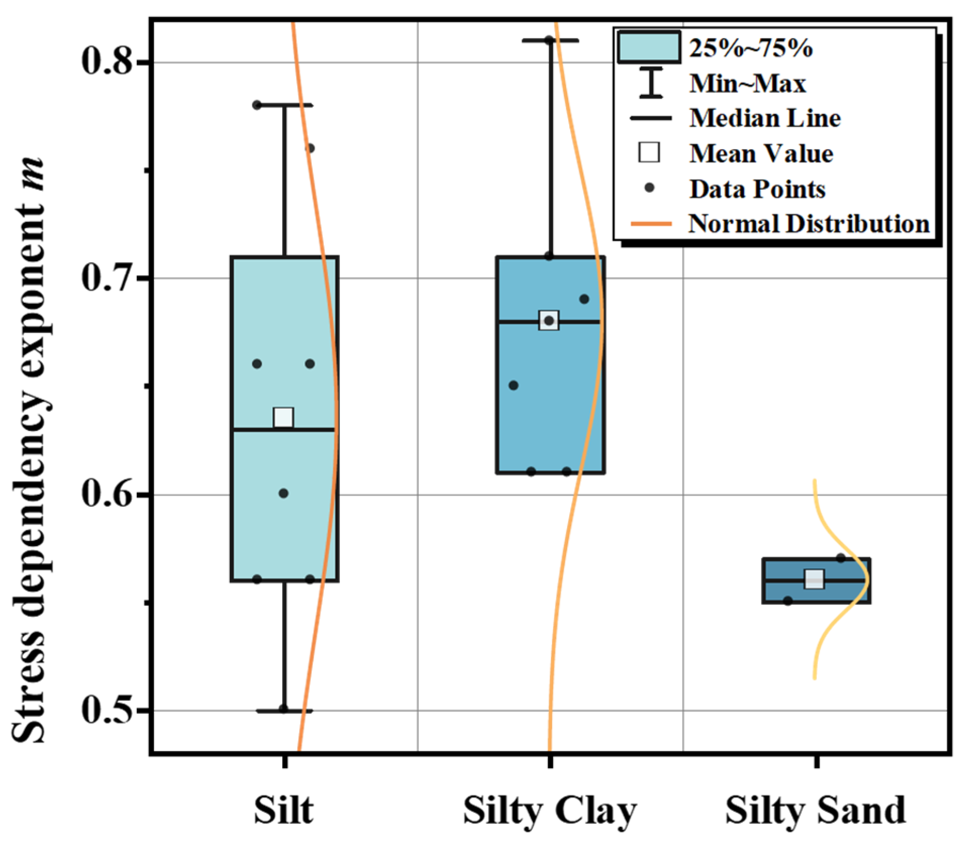
Figure 13 presents the statistical distribution of the stress dependency exponent m, derived from standard consolidation tests for the three typical soil layers (silt, silty clay, and silty sand) in the Taiyuan region. By superimposing normal distribution curves onto box plots, the figure visually reveals both the central tendency and the dispersion characteristics of the experimental data.

Figure 13. Statistical distribution of the stress dependency exponent m for typical soil layers in Taiyuan.

The statistical results indicate that the m values for Taiyuan soils generally range from 0.50 to 0.81, exhibiting significant variations across different lithologies:

Silty Clay: Exhibits the highest stress dependency (μ = 0.68) with a relatively concentrated distribution (0.61–0.81). This narrow range reflects the consistency of the stress response governed by the cohesive soil skeleton structure in this region.

Silt: Shows an intermediate stress dependency (μ = 0.64) but possesses the widest distribution range (0.50–0.78). This significant dispersion highlights its nature as a transitional soil type, characterized by considerable variability in microstructure and particle granulometry.

Silty Sand: Displays the lowest stress dependency (μ = 0.56) with a highly compact distribution (0.55–0.57). This suggests that, in contrast to cohesive soils, the stiffness of this coarse-grained soil is significantly less sensitive to changes in confining pressure.

Overall, all measured m values fall strictly within the empirically recommended range for normally consolidated soils (0.5–1.0). The mean values follow the order of μ_{Silty Clay} > μ_Silt > μ_{Silty Sand}. This trend demonstrates that the stress sensitivity of regional soil stiffness intensifies with increasing fines content.

5. Numerical Verification

5.1. Case Study Overview

5.1.1. Site Description

To validate the reliability of the calibrated parameter system derived in this study, the deep excavation of the Liuxiang Nankou Station on Taiyuan Metro Line 1 was selected for numerical simulation. The selected excavation case was deliberately chosen because it represents a typical deep braced excavation in the Taiyuan area in terms of excavation depth, soil stratification, and support configuration.

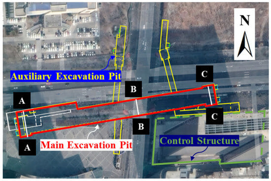
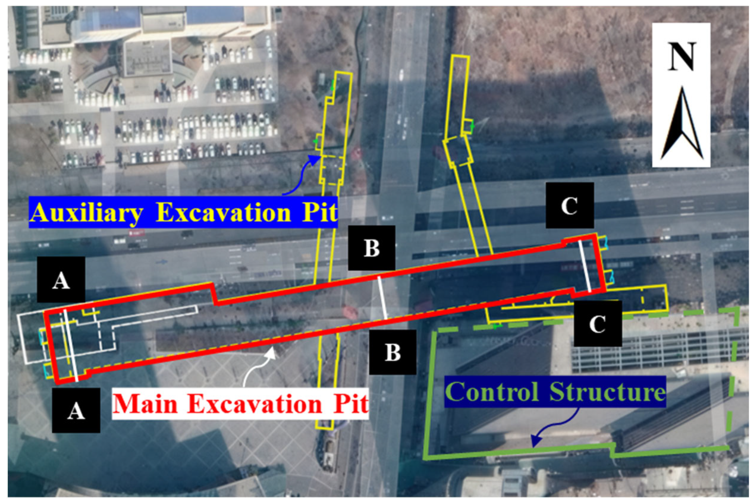
The project is located on the grade I terrace on the east bank of the Fenhe River and was constructed using the cut-and-cover method. The station has a total length of 248 m and includes four entrances/exits and two ventilation pavilions. The construction environment surrounding the excavation is complex, characterized by dense underground pipelines and heavy surface traffic. Notably, a control structure (existing building) is situated to the southeast; its nearest point is only 29 m from the station’s main structure, while its basement is approximately 8.8 m away. The planar location of the station and its surrounding environment are illustrated in Figure 14.

Figure 14. Plan view of the metro station and surrounding environment.

5.1.2. Retaining Structure

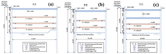
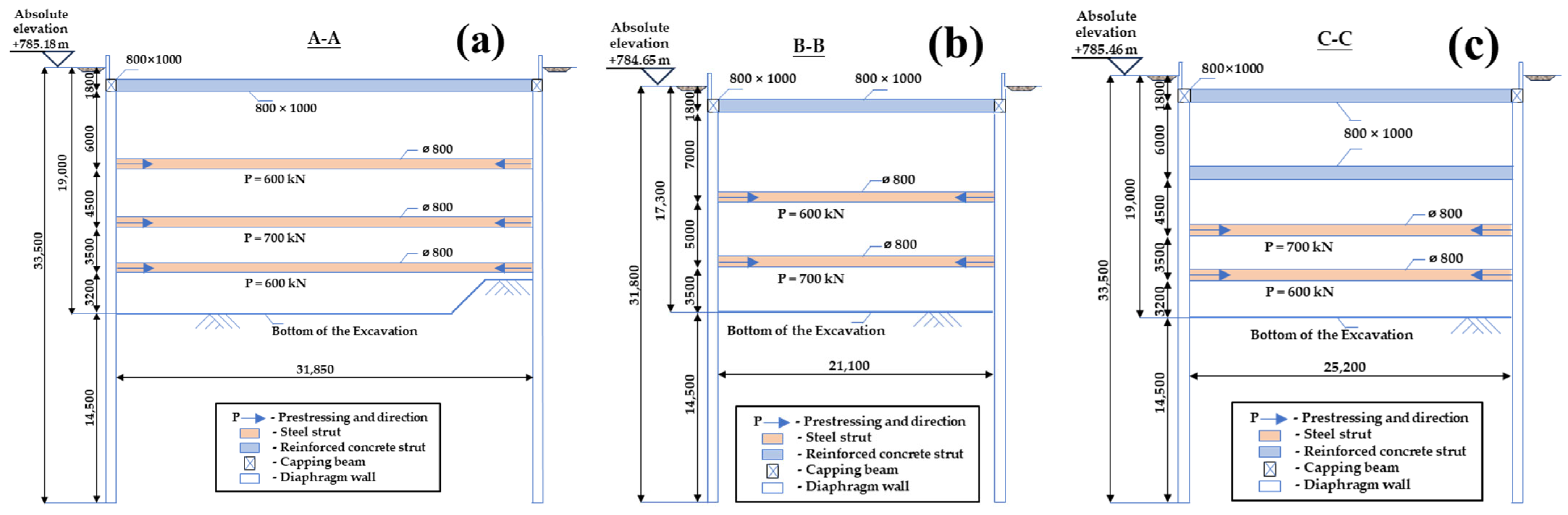
The excavation retaining system adopts a combined support form of “diaphragm wall + internal bracing.” The diaphragm wall consists of a cast-in-place reinforced concrete structure with a thickness of 0.8 m. The first level of support uniformly utilizes reinforced concrete struts with a cross-section of 800 mm × 1000 mm, while the remaining levels employ steel pipe struts (φ = 800 mm, t = 16 mm). Based on the varying widths of the excavation, the station is longitudinally divided into three characteristic sections. The specific support parameters for these sections are detailed in Figure 15.

Figure 15. Cross-sections of the excavation pit (unit: mm). (a) West-end pit (Section A-A). (b) Standard section (Section B-B). (c) East-end pit (Section C-C).

5.1.3. Geological Conditions

The geological environment of the site is typical of the Taiyuan region. The geotechnical investigation report reveals that the groundwater is primarily pore phreatic water, recharged mainly by lateral runoff. The measured stable water level is approximately 3.5 m below the ground surface.

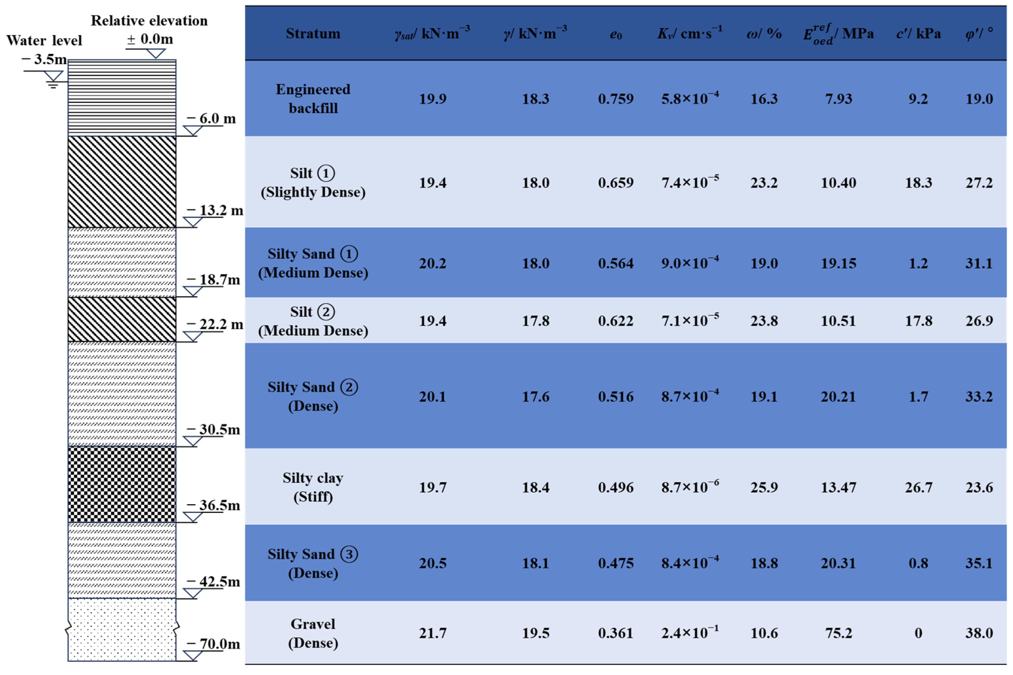
The distribution of soil layers at the site is relatively regular. To ensure the accuracy of the physical and mechanical indicators required for numerical simulation, typical stratigraphic parameters for the standard section (Section B-B) were collated based on the detailed site investigation report. The distribution of soil layers, along with key parameters such as unit weight, void ratio, permeability coefficient, and strength indicators, is presented in Figure 16. These data provide the foundational support for the subsequent establishment of the constitutive model.

Figure 16. Distribution and physical parameters of standard soil layers. Note: γ_sat = saturation unit weight, γ = unit weight, e₀ = initial void ratio, K_v = permeability coefficient, ω = water content, φ′ = effective friction angle, c′ = effective cohesion.

5.1.4. Monitoring Program

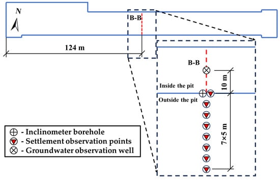
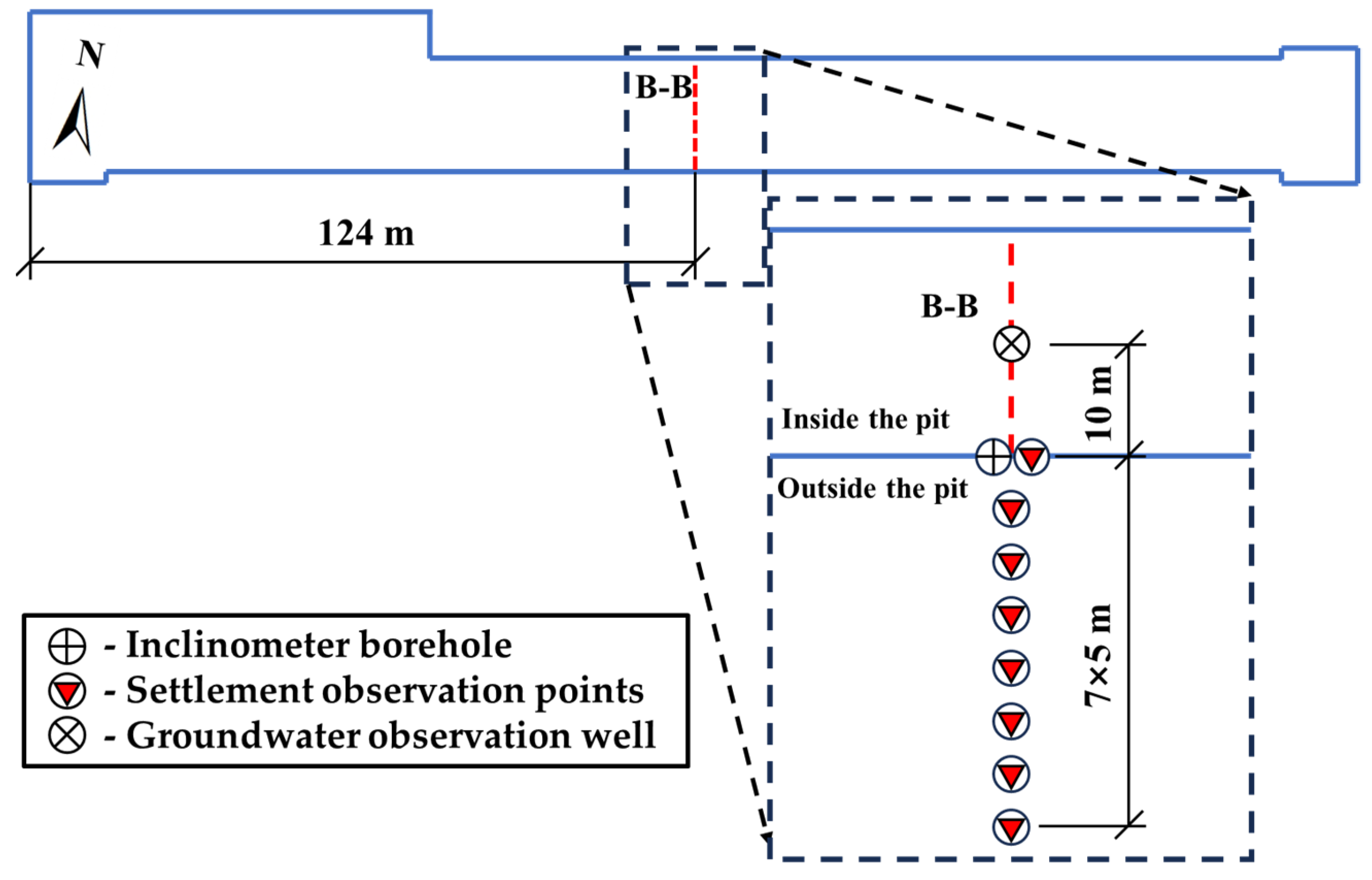
To verify the reliability of the numerical simulation results, the standard section in the middle of the pit (Section B-B) was selected as the representative validation section, as it is minimally affected by spatial end effects. This section is located 124 m from both the east and west ends of the pit, effectively representing the stress and deformation characteristics of the main structure.

The field monitoring focused on the deformation response of the retaining structure and the surrounding ground. Following the principle of symmetrical arrangement, one inclinometer borehole was installed on both the north and south sides of the section to monitor the deep horizontal displacement of the diaphragm wall. Additionally, eight surface settlement observation points were deployed on each side to capture the settlement trough profile behind the wall, and one water level observation well was installed on each side to monitor groundwater fluctuations. This layout achieved comprehensive monitoring and data acquisition throughout the entire excavation process. The detailed monitoring layout at Section B-B is illustrated in Figure 17.

Figure 17. Monitoring layout at Section B-B showing inclinometer boreholes, settlement observation points, and groundwater observation wells.

The selected Section B-B represents the plane strain region of the excavation and was intentionally chosen to minimize corner-induced three-dimensional effects. Although the numerical model accounts for spatial behavior, monitoring data from representative corner sections were not available in the present project. Future studies may incorporate multi-section comparisons to further evaluate corner effects.

5.2. Finite Element Model

5.2.1. Mesh and Boundaries

In this study, the finite element analysis software PLAXIS 3D (Version 25.1) was utilized to simulate the entire excavation process of the metro station deep excavation.

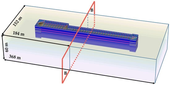
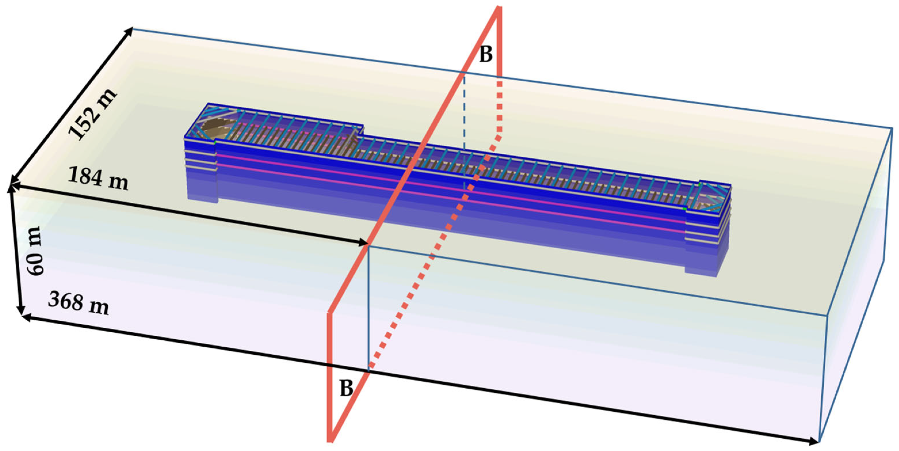
To effectively eliminate boundary effects on the calculation results, the model dimensions were selected based on established recommendations 30, extending approximately 3–4 times the maximum excavation depth in the horizontal direction and 2–3 times in the vertical direction. Given that the station excavation is approximately 248 m long, with a maximum width of 32 m and a depth of 19 m, the final dimensions of the 3D finite element model were determined as 368 m × 152 m × 60 m (Length × Width × Height).

Regarding boundary conditions, the top surface (Z_max) was set as a free surface. Normal displacement constraints were applied to the bottom surface (Z_min) and the four lateral boundaries to simulate roller supports. For hydraulic boundary conditions, the bottom of the model was set as impermeable (Closed), while the top surface and the four lateral boundaries were defined as permeable (Open), allowing for free groundwater seepage to replicate the realistic hydrogeological environment. The established 3D finite element mesh model is shown in Figure 18.

Figure 18. Three-dimensional finite element model of the foundation pit.

5.2.2. Soil Parameters

Based on detailed geotechnical investigation data, the stratigraphic sequence at the central standard section of the excavation, from top to bottom, consists of Engineered Backfill, Silt, Silty Sand (with local intercalated Silty Clay), and Gravel. To meet the computational requirements of finite element simulation, necessary simplifications were introduced: natural soil layers were treated as continuous, horizontal, and isotropic homogeneous materials, and local boulders, lenses, or thin interbeds were merged into the dominant layers.

A category-based assignment strategy was adopted for determining the constitutive model parameters. For the primary soil layers (Silt and Silty Clay), due to the lack of specific advanced soil testing data, the key stiffness indicators for the HSS model were back-calculated using the regional stiffness parameter empirical correlations established in Section 4.1, with the standard constrained modulus from the site investigation report serving as a baseline. Furthermore, the stress dependency exponent m was directly assigned using the regional empirical recommended values derived from the statistical analysis in Section 4.2.

For secondary layers such as Engineered Backfill and Gravel, parameters were estimated based on physical-mechanical statistical indicators from the investigation report and experience from similar engineering projects. The final physical-mechanical indicators and calibrated HSS model parameters for each soil layer are detailed in Table 6.

Table 6. HSS model parameters for each soil layer.

Parameter	Unit	Engineered Backfill	Silt ①	Silty Sand ①	Silt ②	Silty Sand ②	Silty Clay	Silty Sand ③	Gravel
$E_{oed}^{ref}$	MPa	7.93	8.42	19.15	8.51	20.21	12.39	20.31	75.21
$E_{50}^{ref}$	MPa	7.93	9.09	23.55	9.19	24.86	12.39	24.98	75.21
$E_{ur}^{ref}$	MPa	43.62	36.21	78.71	36.59	83.06	50.80	83.47	300.84
m	-	0.50	0.64	0.56	0.64	0.56	0.68	0.56	0.50
$c\prime$	kPa	9.2	18.3	1.2	17.8	1.7	26.7	0.8	0
$\phi \prime$	°	19.0	27.2	31.1	26.9	33.2	23.6	35.1	38.0
$\psi$	°	0	0	1.1	0	3.2	0	5.1	8.0
$R_f$	-	0.9	0.9	0.9	0.9	0.9	0.9	0.9	0.9
$K_0$	-	0.67	0.54	0.48	0.55	0.45	0.60	0.43	0.38
$v_{ur}$	-	0.2	0.2	0.2	0.2	0.2	0.2	0.2	0.2
$P^{ref}$	kPa	100	100	100	100	100	100	100	100
$G_0^{ref}$	MPa	91.71	82.94	121.99	83.82	128.74	146.82	129.37	451.26
${\gamma }_{0.7}$	-	1.0 × 10−4	1.5 × 10−4	2.6 × 10−4	1.5 × 10−4	2.6 × 10−4	1.0 × 10−4	2.6 × 10−4	3.5 × 10−4

5.2.3. Structural Properties

In the PLAXIS 3D model, appropriate structural elements were selected to simulate various components based on their geometric and mechanical characteristics. Specifically, the diaphragm wall was simulated using Plate elements to accurately reflect its soil-retaining, water-blocking, and planar bending properties. Concrete struts, capping beams, and steel walers were modeled using Beam elements to bear axial forces and bending moments. Steel struts were simulated using Node-to-node anchor elements to primarily capture their axial stiffness.

To simplify the calculation, all structural components were assumed to be isotropic linear elastic materials, ignoring plastic deformation. The specific geometric dimensions and physical-mechanical parameters of each structural element are summarized in Table 7.

Table 7. Material properties of each structural element.

Component Name	Element Type	Cross Section /mm	Unit Weight /kN·m−3	Elastic Modulus /MPa
Diaphragm wall	Plate	d = 800	25.0	E1 = E2 = 3.35 × 104
Capping beam	Beam	1000 × 800	25.0	3.35 × 104
Reinforced concrete strut	Beam	1000 × 800	25.0	3.35 × 104
Steel waler	Beam	A = 40,000 mm2	78.5	21 × 104
Steel strut	Node-to-node anchor	D = 800, t = 16	–	21 × 104

Notes: d—thickness of diaphragm wall, A—cross-sectional area of steel waler, D—diameter of steel strut, t—wall thickness of steel strut.

5.2.4. Simulation Sequence

To realistically reproduce the construction process of “layered excavation with concurrent bracing,” a multi-stage continuous analysis method was employed.

This study focuses on validating the calibrated HSS parameters under excavation conditions; therefore, the simulation covers excavation up to the final pit bottom, without considering the post–base slab stage.

Initially, in Phase 0, the K₀ procedure was used to generate the initial in situ stress field. This phase considered only the soil’s self-weight (g = 9.8 m/s²) without tectonic stresses, and the displacement field was reset to zero after equilibrium to eliminate initial deformation caused by gravity loading. Subsequently, the diaphragm wall and capping beam structures were activated to complete the initial setup of the retaining system.

In the subsequent excavation simulation, the sequence strictly followed the construction schedule. “Earthwork excavation” and “Strut installation” were divided into two independent consecutive calculation steps to accurately simulate the stress release upon soil unloading and the time-lag effect of strut activation.

Although long excavation pits are typically constructed in segments (10–20 m wide), sectional excavation was simplified into representative staged steps in the 3D model, since the objective is constitutive parameter validation rather than construction organization simulation. The selected Section B-B is located in the central zone where plane strain conditions dominate, making this simplification acceptable.

Specifically, whenever the excavation reached the design elevation for a support level, a calculation step for dewatering and soil removal was performed first. This was immediately followed by a separate analysis step to activate the corresponding support structure and apply prestress.

Taking the second layer of excavation as an example, the simulation flow was as follows:

• Excavation Step: Groundwater lowering within the pit was simulated via steady-state seepage calculation (setting the boundary head to 1.0 m below the excavation surface), and the soil clusters above this level were deactivated to simulate earthwork removal.
• The steady-state seepage assumption implies full dissipation of pore water pressure within each excavation stage and does not explicitly account for transient groundwater evolution. This simplification was adopted to provide a conservative estimation of excavation-induced deformation and to ensure numerical robustness in multi-stage analysis. The objective is to evaluate structural response under an engineering-relevant hydraulic condition rather than to simulate time-dependent consolidation behavior.
• Support Step: In the subsequent step, the internal bracing components at this elevation (e.g., the second level concrete strut at the east end and the first level steel struts in other areas) were activated. A prestress force of 600 kN was applied to the steel struts according to measured field values. The installation sequence and axial forces are shown in Figure 15.

This “Dewatering/Excavation → Strutting” cycle was repeated for all subsequent layers until the excavation reached the design bottom elevation. The definition of working conditions and water level control for each stage is detailed in Table 8.

Table 8. Three-dimensional finite element analysis steps for excavation.

Phase	Description	Calculation Type	Key Operations	Water Level /m
0	Initial stress	K0 procedure	Activate all soil layers	−3.5
1	Diaphragm wall	Plastic	Activate crown beam and diaphragm wall	−3.5
2	Excavation 1 (Exc 1)	Plastic	Excavate to −1.8 m	−3.5
3	Strut 1	Plastic	Activate 1st strut and waler	−3.5
4	Excavation 2 (Exc 2)	Consolidation	Excavate to −8.8 m, −7.8 m (east and west-end)	−9.8
5	Strut 2	Plastic	Activate 2nd strut and waler	−9.8
6	Excavation 3 (Exc 3)	Consolidation	Excavate to −13.8 m, −12.3 m (east and west-end)	−14.8
7	Strut 3	Plastic	Activate 3rd strut and waler	−14.8
8	Excavation 4 (Exc 4)	Consolidation	Excavate to −17.3 m, −12.3 m (east and west-end)	−18.3
9	Strut 4	Plastic	Activate 4th strut (east and west-end) and waler	−18.3
10	Excavation 5 (Exc 5)	Consolidation	Excavate to −19.0 m (east and west-end)	−20.0

5.3. Validation Results

5.3.1. Lateral Wall Deflection

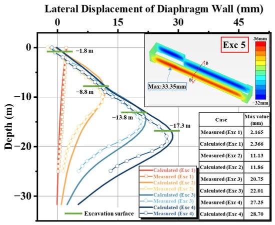
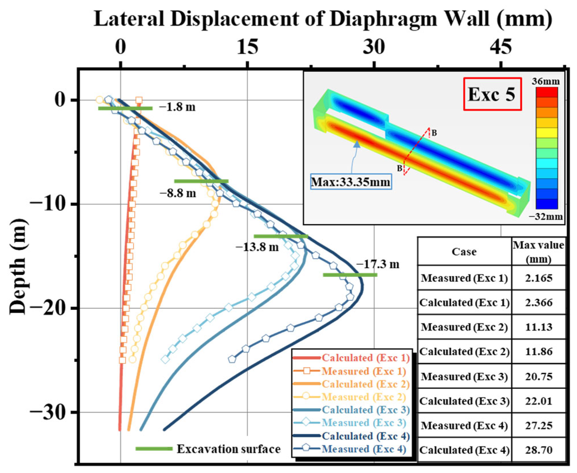
Figure 19 presents a comparison of the deep horizontal displacement curves of the diaphragm wall at Section B-B (south-side inclinometer), obtained from Finite Element Method (FEM) simulations and Field Instrument Monitoring (IM) at different excavation stages (Exc 1 to Exc 4). This monitoring point is located at the representative mid-span section, where corner effects are negligible. The exact location of the inclinometer is illustrated in Figure 17.

Figure 19. Comparison of lateral displacement of the diaphragm wall between FEM and IM at different excavation stages.

Overall, the lateral wall displacement increased with excavation depth, exhibiting distinct spatiotemporal evolution characteristics. In the early stages, the deformation manifested as a “cantilever” mode tilting towards the pit. As excavation deepened and internal struts were installed, this gradually transitioned into a “parabolic” mode (deep inward bulging), with the location of maximum displacement moving progressively deeper.

Quantitatively, the simulation results show high agreement with measured data.

Initial Stage (Exc 1): The maximum lateral movement occurred at the wall top, with an absolute error of only 0.201 mm (relative error 9.3%). Intermediate to Deep Stages (Exc 2–Exc 4): The point of maximum displacement shifted to depths between 8.8 m and 17.8 m below the surface. The absolute error ranged from 0.73 mm to 1.45 mm, with the relative error further decreasing to 5.3–6.6%. Final Stage (Exc 5): The predicted maximum horizontal displacement was 33.35 mm.

The calculated values are slightly larger than the measured ones. This deviation is mainly attributed to the steady-state seepage assumption, which results in more complete pore pressure dissipation within each stage and slightly larger effective stress increments. This represents a conservative estimation.

Overall, the error in maximum wall displacement was consistently controlled within 10%, and the morphological trends of both curves were highly consistent.

5.3.2. Ground Settlement

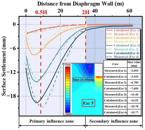
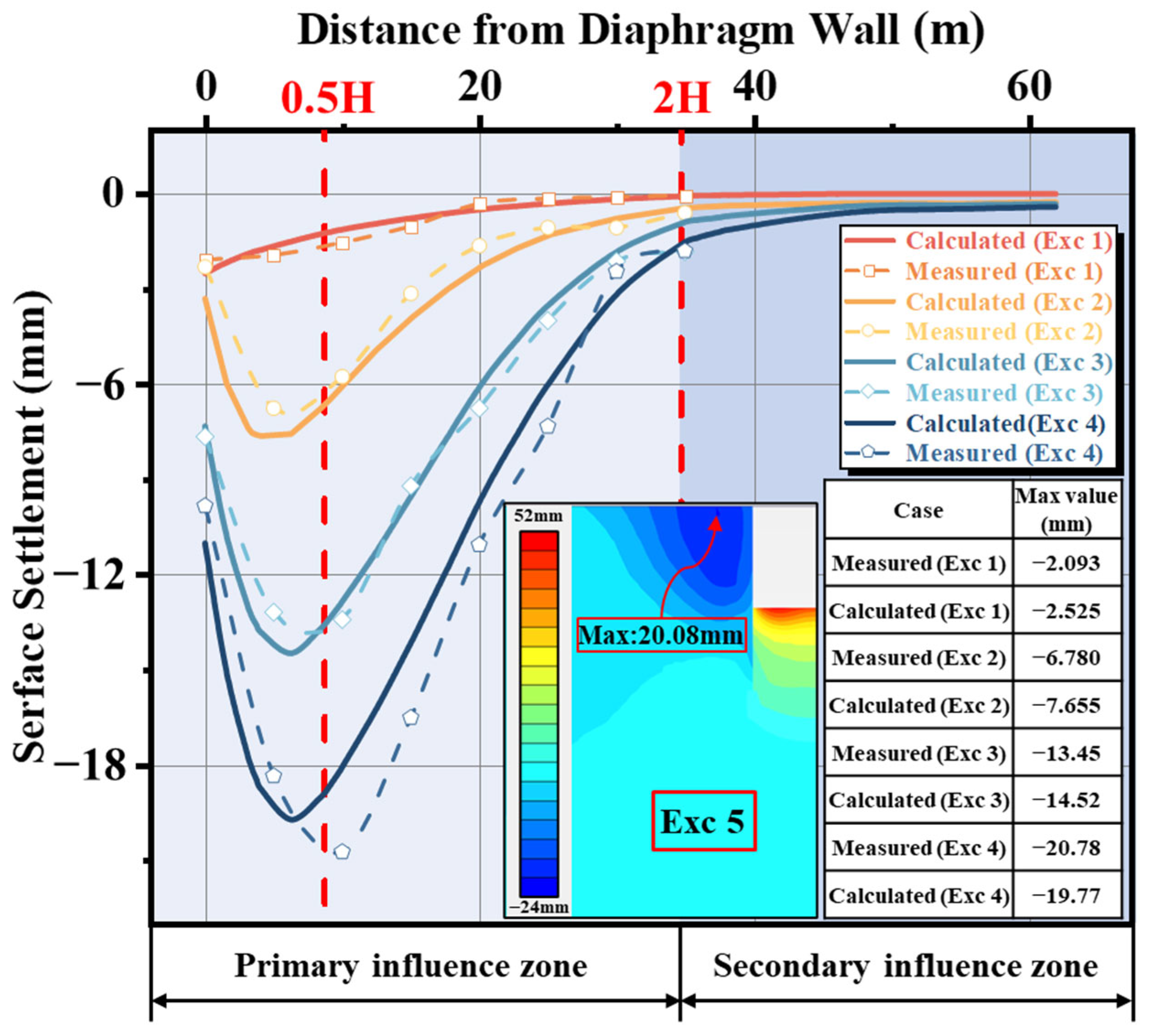
Figure 20 illustrates the evolution of ground surface settlement behind the north side wall, comparing FEM predictions with field monitoring data.

Figure 20. Comparison of surface settlement between FEM and IM at different excavation stages.

Generally, surface settlement accumulated with increasing excavation depth, displaying distinct stage-dependent distribution patterns.

Initial Stage (Exc 1): The settlement profile followed a “triangular” distribution, with maximum settlement occurring at the wall edge (0.00 m). Subsequent Stages (Exc 2–Exc 4): The profile gradually evolved into a typical “groove-type” settlement trough. Based on the settlement gradient, the ground surface can be divided into a primary influence zone (0–2.0 H, where H is excavation depth) and a secondary influence zone (2.0 H–4.0 H). Monitoring data indicates that the peak settlement point migrated away from the pit, eventually stabilizing at approximately 0.5 H from the wall edge.

From a numerical perspective, although the relative error in the initial stage (Exc 1) appeared large (20.6%) due to the extremely small measured value (only 2.093 mm), the absolute error was merely 0.432 mm, falling well within permissible measurement error limits. As excavation progressed to deeper levels, the model’s prediction accuracy improved significantly. During stages Exc 2 to Exc 4, the simulated location of maximum settlement matched the field data well, both falling within the primary influence zone. The relative error of the maximum settlement decreased sequentially to 12.9%, 8.0%, and 4.9%. Notably, in the final stage (Exc 4), the predicted maximum settlement was 19.77 mm, highly consistent with the measured 20.78 mm, verifying the model’s capability in predicting large deformations.

Regarding the systematic deviation where simulated values slightly exceeded measured ones (except for the final stage), the cause is consistent with that of the wall displacement error: the steady-state seepage assumption in the numerical model is more conservative than the actual transient non-steady flow, leading to calculated effective stress increments and consolidation settlements that are slightly larger than observed. Overall, excluding the initial minor deformations, the calculation error for maximum surface settlement was consistently controlled within 13%, and the width and shape of the settlement trough aligned closely with field results. This demonstrates that the HSS model and the selected parameters effectively reflect the complex deformation behavior of the soil behind the wall under unloading paths.

The results demonstrate that the HSS parameters, derived from the empirical formulas in Section 4, accurately capture the non-linear deformation characteristics of the deep excavation system. Consequently, the established numerical model proves to be highly reliable and suitable for engineering applications in the Taiyuan region.

6. Conclusions

This study investigated the geotechnical properties of typical soils (silt, silty clay, and silty sand) in the Taiyuan region. Through laboratory testing, the ranges of key HSS model stiffness parameters were determined, and regional stiffness proportional relationships were established. Subsequently, the derived parameter system was applied to the numerical simulation of a deep metro station excavation and validated against field monitoring data. The main conclusions are as follows:

(1)

A complete set of stiffness parameters ($E_{oed}^{ref}$, $E_{50}^{ref}$, $E_{ur}^{ref}$, $G_0^{ref}$) for typical soils in the Taiyuan region was obtained across the full strain range. Results confirm that the HSS model accurately captures the non-linear deformation characteristics of local soils under various stress paths.

(2)

Based on zero-intercept linear regression analysis, normalized stiffness parameter ratios ($E_{oed}^{ref}$: $E_{50}^{ref}$: $E_{ur}^{ref}$: $G_0^{ref}$) were established for the three typical soil types. Specifically, the ratio is 1.00:1.08:4.30:9.85 for silt, 1.00:1.00:4.10:11.85 for silty clay, and 1.00:1.23:4.11:6.37 for silty sand. These empirical relationships quantitatively reveal the evolution laws from static large-strain stiffness to dynamic small-strain stiffness and provide regional reference values for preliminary HSS parameter calibration, particularly in the absence of advanced testing conditions.

(3)

The stress dependency exponent m ranges from 0.50 to 0.81. Mean values follow the order: μ_{Silty Clay} (0.68) > μ_Silt (0.64) > μ_{Silty Sand} (0.56). This trend indicates that stress sensitivity increases with higher fines content. All measured values fall within the recommended range for normally consolidated soils.

(4)

Numerical simulations showed high agreement with field monitoring data. During key construction stages, maximum errors for lateral wall displacement were within 10%. Similarly, surface settlement errors were controlled within 13%. This verifies the engineering applicability of the proposed parameter system. It should be noted that the proposed parameter system is validated based on a representative excavation case, and further verification using additional projects will be conducted in future studies.

(5)

The numerical analysis successfully reproduced the transition from “cantilever” to “parabolic” wall deformation and the “groove-type” settlement trough. Calculated results were slightly larger than measured values due to the conservative steady-state seepage assumption. This deviation provides a beneficial safety margin for engineering design.

While this study focused on silt, silty clay, and silty sand, future research will encompass a broader range of soil categories to systematically establish regional HSS parameter laws. Furthermore, element-level numerical simulations in PLAXIS 3D will be performed to compare stress–strain responses, failure envelopes, and stress path evolution with laboratory results, thereby enhancing the robustness of the calibrated parameter system. Ultimately, these efforts will facilitate the development of a more universally applicable and practical framework for parameter selection.

References

- Hsieh, P.-G.; Ou, C.-Y. Shape of Ground Surface Settlement Profiles Caused by Excavation. Can. Geotech. J. 1998, 35, 1004–1017. [Google Scholar] [CrossRef]
- Zeng, C.-F.; Wang, S.; Xue, X.-L.; Zheng, G.; Mei, G.-X. Characteristics of Ground Settlement Due to Combined Actions of Groundwater Drawdown and Enclosure Wall Movement. Acta Geotech. 2022, 17, 4095–4112. [Google Scholar] [CrossRef] [Scilit]
- Zhao, C.; Cheng, Y.; Zeng, G.; Lu, G.; Ju, Y. Experimental Investigation of Soil Settlement Mechanisms Induced by Staged Dewatering and Excavation in Alternating Multi-Aquifer–Aquitard Systems. Buildings 2025, 15, 1534. [Google Scholar] [CrossRef] [Scilit]
- Alzabeebee, S. Numerical Analysis of the Interference of Two Active Machine Foundations. Geotech. Geol. Eng. 2020, 38, 5043–5059. [Google Scholar] [CrossRef] [Scilit]
- Pi, J.; Xu, Y.; Zhang, J.; Du, Z.; Zeng, Y. Experimental Determination of HSS Model Parameters for Typical Zhengzhou Strata and Their Application in Shield Tunnel Construction. Front. Earth Sci. 2025, 13, 1598049. [Google Scholar] [CrossRef] [Scilit]
- Hu, J.; Du, Q. Parameter Study and Engineering Verification of the Hardening Soil Model with Small-Strain Stiffness for Loess in the Xi’an Area. Appl. Sci. 2025, 15, 1278. [Google Scholar] [CrossRef] [Scilit]
- Arkinsos, J.H.; Sallfors, G. Experimental Determination of Soil Properties. In Proceedings of the 10th ECSMFE, 1991; Volume 3, pp. 915–956. Available online: https://www.scirp.org/reference/referencespapers?referenceid=3031068 (accessed on 9 February 2026).
- Cudny, M.; Truty, A. Refinement of the Hardening Soil Model within the Small Strain Range. Acta Geotech. 2020, 15, 2031–2051. [Google Scholar] [CrossRef] [Scilit]
- Jardine, R.J.; Potts, D.M.; Fourie, A.B.; Burland, J.B. Studies of the Influence of Non-Linear Stress–Strain Characteristics in Soil–Structure Interaction. Geotechnique 1986, 36, 377–396. [Google Scholar] [CrossRef] [Scilit]
- Roscoe, K.H.; Burland, J.B. On the Generalized Stress-Strain Behaviour of Wet Clay. In Engineering Plasticity; Cambridge University Press: Cambridge, UK, 1968. [Google Scholar]
- Schanz, T.; Vermeer, P.A.; Bonnier, P.G. The Hardening Soil Model: Formulation and Verification. In Beyond 2000 in Computational Geotechnics; Routledge: Oxfordshire, UK, 1999. [Google Scholar]
- Ardakani, A.; Bayat, M.; Javanmard, M. Numerical modeling of soil nail walls considering Mohr Coulomb, hardening soil and hardening soil with small-strain stiffness effect models. Geomech. Eng. 2014, 6, 391–401. [Google Scholar] [CrossRef] [Scilit]
- Benz, T. Small-Strain Stiffness of Soils and Its Numerical Consequences; Institut für Geotechnik der Universität Stuttgart: Stuttgart, Germany, 2007; Volume 5. [Google Scholar]
- Hardin, B.O.; Drnevich, V.P. Shear Modulus and Damping in Soils: Design Equations and Curves. J. Soil Mech. Found. Div. 1972, 98, 667–692. [Google Scholar] [CrossRef] [Scilit]
- Benz, T.; Vermeer, P.A.; Schwab, R. A Small-Strain Overlay Model. Int. J. Numer. Anal. Methods Geomech. 2009, 33, 25–44. [Google Scholar] [CrossRef] [Scilit]
- Wang, T.; Deng, T.; Deng, Y.; Yu, X.; Zou, P.; Deng, Z. Numerical Simulation of Deep Excavation Considering Strain-Dependent Behavior of Soil: A Case Study of Tangluo Street Station of Nanjing Metro. Int. J. Civ. Eng. 2023, 21, 541–550. [Google Scholar] [CrossRef] [Scilit]
- Hsiung, B.-C.B.; Dao, S.-D. Evaluation of Constitutive Soil Models for Predicting Movements Caused by a Deep Excavation in Sands. Electron. J. Geotech. Eng 2014, 19, 17325–17344. [Google Scholar]
- Sadiq, S.; Won, M.-S.; Kim, H.J.; Hong, C. Hybrid Finite Element and Machine Learning Approach for Estimating Lateral Capacity of Partially Rock-Socketed Monopiles. Ocean Eng. 2025, 330, 121286. [Google Scholar] [CrossRef] [Scilit]
- Sadiq, S.; Kim, H.-J.; Won, M.-S.; Park, Y.-C. A Qualitative Study on the Lateral Behavior of Rock-Socketed Monopiles. Mar. Struct. 2025, 104, 103892. [Google Scholar] [CrossRef] [Scilit]
- Li, L.; Liu, J.; Li, K.; Huang, H.; Ji, X. Study of Parameters Selection and Applicability of HSS Model in Typical Stratum of Jinan. Rock Soil Mech. 2019, 40, 4021–4029. [Google Scholar] [CrossRef]
- Mu, L.; Huang, M. Small Strain Based Method for Predicting Three-Dimensional Soil Displacements Induced by Braced Excavation. Tunn. Undergr. Space Technol. 2016, 52, 12–22. [Google Scholar] [CrossRef] [Scilit]
- Gu, X.Q.; Wu, R.T.; Liang, F.Y.; Gao, G.Y. On HSS Model Parameters for Shanghai Soils with Engineering Verification. Rock Soil Mech. 2021, 42, 833–845. [Google Scholar] [CrossRef]
- Fu, Y.; He, S.; Zhang, S.; Yang, Y. Parameter Analysis on Hardening Soil Model of Soft Soil for Foundation Pits Based on Shear Rates in Shenzhen Bay, China. Adv. Mater. Sci. Eng. 2020, 2020, 7810918. [Google Scholar] [CrossRef] [Scilit]
- Du, Z.; Zhang, Z.; Wang, L.; Zhang, J.; Li, Y. Effect of Moisture Content on the Permanent Strain of Yellow River Alluvial Silt under Long-Term Cyclic Loading. Sustainability 2023, 15, 13155. [Google Scholar] [CrossRef] [Scilit]
- Bolton, M.D. Discussion: The Strength and Dilatancy of Sands. Géotechnique 1987, 37, 219–226. [Google Scholar] [CrossRef] [Scilit]
- Wang, W.D.; Wang, H.R.; Xu, Z.H. Experimental Study of Parameters of Hardening Soil Model for Numerical Analysis of Excavations of Foundation Pits. Rock Soil Mech. 2012, 33, 2283–2290. [Google Scholar] [CrossRef]
- Yang, L.; Zhou, L.; Xia, W.; Guan, R.Q.; Zhang, H.; Luo, W.J. Experimental Study of Parameters of HS Model for Numerical Analysis of Foundation Pits in Ningbo Soft Soil Area. Tunn. Constr. 2018, 38, 954–962. [Google Scholar] [CrossRef]
- Chen, Y.; Shen, D.; Luo, M.; Huang, J.; Shen, P. Experimental Research and Application of Small-Strain Soil Hardening Model Parameters in a Major Project in Hangzhou. Transp. Res. Rec. J. Transp. Res. Board 2024, 2678, 1939–1949. [Google Scholar] [CrossRef] [Scilit]
- Dong, X.; Zhou, F.; Zhu, R.; Wang, X.-D.; Zeng, L.-Y. Sensitivity Analysis and Determination Method of Parameters for Hardening Soil Model with Small Strain Stiffness. Sci. Technol. Eng. 2024, 24, 6366–6376. [Google Scholar]
- Shi, X.; Sun, J.; Qi, Y.; Zhu, X.; Zhang, X.; Liang, R.; Chen, H. Study on Stiffness Parameters of the Hardening Soil Model in Sandy Gravel Stratum. Appl. Sci. 2023, 13, 2710. [Google Scholar] [CrossRef] [Scilit]
- Fernández-Ruiz, J.; Pereira, C. Non-Linear Critical Speed in High-Speed Ballasted Railways with Ground Reinforcement. Transp. Geotech. 2024, 48, 101325. [Google Scholar] [CrossRef] [Scilit]
- Brinkgreve, R.B.J.; Kappert, M.H.; Bonnier, P.G. Hysteretic Damping in a Small-Strain Stiffness Model. In Proceedings of the 10th International Symposium on Numerical Models in Geomechanics (NUMOG X), Rhodes, Greece, 25–27 April 2007; Taylor & Francis: Abingdon, UK, 2007; pp. 737–742. [Google Scholar]
- Silva, F.; Gomes, R.C. Importance of Small-Strain Stiffness on the Prediction of the Displacements of a Flexible Retaining Wall on Stiff Clay. In Proceedings of the 17th European Conference on Soil Mechanics and Geotechnical Engineering, ECSMGE 2019; International Society for Soil Mechanics and Geotechnical Engineering: London, UK, 2019. [Google Scholar]
- Kim, T.; Jung, Y.-H. Optimizing Material Parameters to Best Capture Deformation Responses in Supported Bottom-up Excavation: Field Monitoring and Inverse Analysis. KSCE J. Civ. Eng. 2022, 26, 3384–3401. [Google Scholar] [CrossRef] [Scilit]
- ASTM D2435/D2435M-25; Standard Test Methods for One-Dimensional Consolidation Properties of Soils Using Incremental Loading. ASTM International: West Conshohocken, PA, USA, 2025. [CrossRef] [Scilit]
- ASTM D4767-11(2020); Standard Test Method for Consolidated Undrained Triaxial Compression Test for Cohesive Soils. ASTM International: West Conshohocken, PA, USA, 2020. [CrossRef] [Scilit]
- ASTM D4015-21; Standard Test Methods for Modulus and Damping of Soils by Fixed-Base Resonant Column Devices. ASTM International: West Conshohocken, PA, USA, 2021. [CrossRef] [Scilit]
- Bentley Systems. PLAXIS 3D Material Models Manual; Bentley Systems, Inc: Exton, PA, USA, 2025. [Google Scholar]
- Santos, J.A.; Correia, A.G. Shear Modulus of Soils under Cyclic Loading at Small and Medium Strain Level. In Proceedings of the 12th World Conference On Earthquake Engineering, Auckland, New Zealand, 30 January–4 February 2000; Volume 530, pp. 90–98. [Google Scholar]
- Vucetic, M.; Dobry, R. Effect of Soil Plasticity on Cyclic Response. J. Geotech. Eng. 1991, 117, 89–107. [Google Scholar] [CrossRef] [Scilit]
- Darendeli, M.B. Development of a New Family of Normalized Modulus Reduction and Material Damping Curves; The University of Texas at Austin: Austin, TX, USA, 2011. [Google Scholar]
Disclaimer/Publisher’s Note: The statements, opinions and data contained in all publications are solely those of the individual author(s) and contributor(s) and not of MDPI and/or the editor(s). MDPI and/or the editor(s) disclaim responsibility for any injury to people or property resulting from any ideas, methods, instructions or products referred to in the content. |
© 2026 by the authors. Licensee MDPI, Basel, Switzerland. This article is an open access article distributed under the terms and conditions of the Creative Commons Attribution (CC BY) license.