


Abstract
Indoor Air Quality (IAQ) is a factor correlated with the comfort and health of occupants. The development of financially accessible monitoring systems facilitates the continuous evaluation of conditions in indoor spaces. The paper proposes the evaluation of a low-cost IoT architecture for monitoring environmental parameters and producing a sensor-derived estimated AQI through machine learning techniques. The prototype, costing 56.85 USD, utilizes the M5Stack Core2 platform and the ENV Pro module based on the BME688 sensor for acquiring temperature, relative humidity, volatile organic compounds, and the estimated CO2 value. The data is transmitted to an Azure infrastructure, which integrates services for data storage and model inference. For the development of the predictive component, the public DALTON dataset was used. From this dataset, 2,401,750 observations corresponding to office-type spaces were selected. The regression models used temperature, relative humidity, CO2, and VOC as input variables. The target variable was the AQI. The model estimates the AQI based on temperature, relative humidity, CO2, and VOC, without using PM2.5 and PM10 as predictors. These two parameters were not included as predictors to avoid the direct use of the variables from which the target is calculated in the model. The research compares two training environments, locally through ML.NET and in the cloud through Azure Machine Learning. The LightGBM model trained locally achieved the best performance. The full dataset goodness-of-fit diagnostics were: R2 = 0.998513, MAE = 0.552383, RMSE = 0.964316, and a Spearman correlation of 0.998814. The main contribution consists of integrating a low-cost embedded node, Azure services, and a regression model into an operational workflow. Its objective is the acquisition, transmission, storage, inference, and display of the result. The study demonstrates the functioning of this architecture.
1. Introduction
Indoor air quality (IAQ) is a component that influences public health. People spend a large part of their time in enclosed spaces. Inappropriate values associated with IAQ generate long-term negative effects on health. For the synthetic expression of pollution levels, the Air Quality Index (AQI) is used, which is specific to outdoor air. IAQ integrates the measured values of pollutant concentrations into an indicator that can be interpreted in relation to the pollution level. The index can be determined based on the values provided by different sensors that measure pollutant levels.
IAQ and AQI are different concepts. IAQ is a generalization of air quality within buildings. Its value simultaneously takes into account pollutants, ventilation, and comfort parameters. AQI is a numerical or categorical indicator that indicates a certain level of pollution based on pollutant concentrations. AQI is primarily used for outdoor air. It can be adopted for indoor spaces on the condition that the pollutants included in the calculation are defined.
The model output is termed sensor-derived estimated AQI, with a training target calculated exclusively from PM2.5 and PM10. IAQ denotes the broader monitoring context. The EPA framework also considers ozone, CO, SO2, and NO2 [1]. CO2 instead provides contextual information about occupancy and ventilation. The restricted output does not assess overall IAQ or health risks.
The specialized literature studies the issue of IAQ in relation to professional devices, proposing various solutions that offer reduced costs and similar performance. According to the source [2], in 2021, household air pollution was associated with 2.9 million premature deaths, contributing to the worldwide burden of household air pollution. Over 300,000 deaths were recorded among children under 5 years old. The effects of outdoor air pollution and household air pollution are associated with approximately 6.7 million premature deaths annually [2].
Chojer et al. [3] conducted a review of the specialized literature, in which the monitored IAQ parameters through low-cost devices are synthesized. The parameters recorded in the study are temperature, relative humidity (RH), carbon dioxide (CO2), carbon monoxide (CO), ozone (O3), nitrogen dioxide (NO2), Volatile Organic Compound (VOC)/Total Volatile Organic Compounds (TVOCs), particulate matter with an aerodynamic diameter below 2.5 µm (PM2.5), particulate matter with an aerodynamic diameter below 10 µm (PM10), and formaldehyde, as well as indoor comfort variables such as illumination, noise, air velocity, and occupancy. Table 1 presents a synthesis of the parameters monitored in several studies regarding IAQ. Additionally, Table 1 also depicts the sensors used in the research.
Table 1.
Parameters monitored for IAQ in different studies, along with the research context and the sensors used.
Table 1 highlights the type of indoor space monitored, measured parameters, and hardware configuration. Sá et al. [4] applies a field comparison with research instruments and reports data losses, connectivity issues, erroneous values, and differences between devices. In the research by Tran et al. [5], the AirVisual device was used for indoor PM2.5, PurpleAir was used for outdoor PM2.5, and DustTrak II 8530 was the reference instrument used for calibration in five urban households.
The studies included in Table 1 were selected through a search in the Web of Science Core Collection that included the terminology “indoor air” in relation to quality, “Internet of Things”, “low-cost sensor”, architectural-level monitoring criteria, and a dedicated microcontroller-based platform, with a year restriction associated with the publication of materials after 2020, to analyze the latest research in the field. The literature overview is selective rather than exhaustive.
The devices presented in Table 1 belong to two different categories. The first category corresponds to IAQ monitoring systems integrated into IoT infrastructures. AirVisual Pro (manufactured by IQAir AG, Goldach, Switzerland), Airthings View Plus (manufactured by Airthings ASA, Oslo, Norway), PurpleAir (manufactured by PurpleAir, Inc., Bluffdale, Utah, USA), PocketLab Air (manufactured by Myriad Sensors Inc, San Jose, CA, USA), Smart Citizen Kit (manufactured by Fab Lab Barcelona / IAAC, Barcelona, Spain), and uRAD Monitor A3 (manufactured by Magnasci SRL, Timisoara, Romania) are suitable devices for IAQ monitoring in homes, schools, offices, hospitals, and public spaces. They measure PM2.5, PM10, CO2, temperature, and RH, and some include VOC, O3, formaldehyde, pressure, noise, or radon.
In order to estimate IAQ, different machine learning (ML) models are applied to data supplied by various environmental sensors, such as PM2.5, PM10, CO, CO2, NO2, VOC, temperature, and RH, as can be seen in Table 1. Based on our synthesis of the studies reviewed below, the recent literature can be organized into four main research directions: classical and ensemble ML, deep learning, hybrid architectures, and interpretable ML.
Ensemble tree-based models (eXtreme Gradient Boosting—XGBoost, Random Forest—RF, Gradient Boosting—GB, Light Gradient Boosting Machine—LightGBM) are used both for low-cost sensor calibration (achieving an R2 up to 0.97 for CO2, PM2.5, temperature and RH [23]), for direct pollutant regression (RF explaining indoor PM2.5 with an R2 of 0.84 [24]), and also for CO2 estimation from temperature/humidity (with an R2 of 0.89 when no CO2 sensor is available [25]). Support Vector Machine (SVM) and k-Nearest Neighbor (kNN) methods supply good results for classification-based AQI prediction, with accuracies of 80–99% in kitchen [26] and cabin [27] environments, and for gas-sensor calibration, where SVR outperformed the alternative methods for CO, NO2 and O3 estimation in classrooms [7].
For CO2 forecasting, Long Short-Term Memory (LSTM) variants (including attention-based [28] and RF/Tree-Structured Parzen Estimator (TPE)-optimized LSTM [29]) achieve mean absolute error (MAE) values of 2.96–8.9 ppm at short prediction horizons, consistent across hospital [28] and classroom [29] settings. For particulate matter, hybrid ML models such as LightGBM–Gated Recurrent Unit (GRU) [30] and Seasonal-Trend decomposition using Loess (STL) combined with meta-learning [31] supply better performance than single-model approaches, with reported mean absolute percentage error (MAPE) as low as 1.76% [30] and PM10 forecasting accuracy of 94.93% [31]. Also, GRU was identified as a computationally efficient alternative to LSTM for public-building microclimate studies [32].
An emerging research direction combines predictive models with SHapley Additive exPlanations (SHAP) interpretability in order to identify the specific predictors of indoor pollutant levels (rather than treating the model as a black box): outdoor PM1 and PM2.5 infiltrations and building airtightness are identified as main predictors in residential settings [33], in households [24], and in higher-education buildings [34]. A limited number of studies scale ML-based indoor estimation to the population level (R2 of 0.71–0.89), estimating indoor PM2.5 for entire city networks [35] or during wildfire seasons [36].
A gap relevant to comparing local versus cloud ML for low-cost embedded IAQ devices is that only a few studies explicitly evaluate computational feasibility on low-cost embedded hardware versus cloud inference, despite most proposed frameworks (hybrid LSTM-GRU with Neural Networks (NNs) [37], attention-based LSTM [28], and physics-informed XGBoost [38]) being computationally demanding.
Table 2 presents a selection of ML and DL models applied to monitoring (including estimation and forecasting) of indoor air quality parameters (PM2.5, PM10, PM1, NO2, CO, CO2, VOC, RH, and temperature), using the following criteria: method, applicability, analyzed environmental parameters, R2, MAE, and root mean squared error (RMSE) reported values. It must be mentioned that only studies that report at least one quantitative R2, MAE, and RMSE were included.
Table 2.
ML and DL models applied to the indoor air quality parameters monitoring.
The R2, MAE, and RMSE values in Table 2 are presented as reported by the source studies and must be interpreted solely in the context of each study’s specific target, unit, environment, and validation protocol. They are not used for a direct numerical ranking comparing CO2 prediction, particle regression, sensor calibration, and the other tasks. The comparative summary relevant to this paper is structured in Table 3 according to model family, merits, limitations, and scope of application.
Table 3.
Comparative synthesis of the merits and limitations of the main families of models identified in the analyzed literature.
The cited studies report different targets and evaluation protocols, including CO2 prediction in ppm and PM prediction in concentration units. Their R2 values are illustrative dataset-specific results.
The paper proposes a low-cost Internet of Things (IoT) sensing node and evaluates an exploratory methodological approach for producing a sensor-derived estimated AQI. It aims to monitor IAQ by collecting indirect environmental parameters, transmitting them, and storing them in the cloud, as well as producing a sensor-derived estimated AQI through machine learning ML models. Extremely important for this research is the differentiation between AQI and IAQ. In this paper, the AQI training target is calculated from particulate matter concentrations, while temperature, RH, CO2, and VOC are used to produce the sensor-derived estimated AQI. IAQ denotes the broader indoor environmental context.
The specific objectives of this work are:
- The proposal of an embedded prototype consisting of the M5Stack Core2 platform and the ENV Pro module with the BME688 sensor (manufactured by M5Stack Technology Co., Ltd., Shenzhen, China).
- Development of an IoT flow capable of acquiring data, facilitating preprocessing, transmission, storage, and display of data to devices.
- Preparing DALTON data for an exploratory evaluation using four prototype-related predictors.
- Development of regression models for estimating AQI based on temperature, RH, CO2, and VOC.
- Comparing the performance of local training, conducted with ML.NET Model Builder, against cloud training, conducted through Azure ML.
- Integrating the DALTON model into the prototype to demonstrate the operational inference workflow.
- Displaying the sensor-derived estimated AQI on the M5Stack Core2 device in a user-friendly graphical format.
The research objectives are: formulating the regression problem, evaluating candidate models in the declared protocols, analyzing the integration of the selected model, building an experimental prototype that uses the model, implementing the IoT flow, and storing and displaying the data on which the technical functioning of the architecture is demonstrated.
The main contribution of the authors lies in the development of a modular cyber-physical architecture that integrates embedded hardware components, Azure services, Structured Query Language (SQL) and Cosmos DB databases, and ML models into a unified operational flow. The proposed monitoring prototype is acquired at a cost of 56.85 USD. It can be extended in the future to monitor larger and different indoor spaces.
From a methodological standpoint, the paper proposes a sensor-derived estimated AQI using temperature, RH, CO2, and VOC, with a training target calculated from PM2.5 and PM10. The decision to integrate in such a manner avoids introducing into the model the variables from which AQI is calculated based on the formula, thus implicitly avoiding the triviality of the prediction problem.
Other contributions focus on a descriptive comparison of local and cloud infrastructures under non-equivalent search budgets. The study records metrics and proposes a method for integrating the selected model into an infrastructure that can be accessed from anywhere, provided there is access to the internet. Thus, the prediction can be reused at the level of the M5Stack Core2 device. The original contribution of the study lies in the implementation and functional demonstration of an experimental setup for monitoring indoor environmental parameters. This connects an M5Stack Core2 node, equipped with the ENV Pro module based on the BME688 sensor, to Azure services for data transmission, processing, storage, executing inference, and returning the result for display on the device. The contribution consists of integrating these components and existing ML methods into a unified operational flow. The acquisition cost of the prototype is contextualized by comparing it with the prices of systems presented in the specialized literature. The predictive component explores the estimation of an index derived from the concentrations of PM2.5 and PM10. The demonstration of operational integration is limited by the validation of the accuracy of the estimates and the transferability of the model to the prototype data.
The research is part of an internal grant project dedicated to the study of IAQ through modern techniques. In this category of techniques, there are proposals for IoT infrastructures, embedded systems, cloud services, ML, specific data processing and storage mechanisms, etc. In this context, the paper aimed to develop a complete experimental infrastructure and represents a continuation of the authors’ other specialized works in the same field. In a previous study [39], the authors proposed a software solution for predicting and forecasting urban AQI. Additionally, the authors of this paper have also conducted a systematic analysis of the datasets and algorithms used in IAQ research [40]. The authors have also investigated the indirect machine learning prediction of a composite indoor air quality index in an airport passenger transit area [41] demonstrating the continuity of their research on sensor-based IAQ monitoring and data-driven analysis.
2. Materials and Methods
The main objective of this research is to design and implement a system that measures environmental parameters in indoor spaces and displays the sensor-derived estimated AQI on the proposed prototype’s screen. As shown in the literature review section, there is no single, universally accepted indicator for expressing IAQ in the form of a generalized score. In this paper, IAQ designates the general concept of indoor air quality. This includes thermal comfort, ventilation, the presence of pollutants, occupancy levels, and other factors that contribute to the degradation of air quality. In contrast, the model’s output is called AQI, as the training target is calculated exclusively from PM2.5 and PM10. The model uses only temperature, relative humidity, CO2, and VOC as predictors. Therefore, the result does not represent a complete index of IAQ. Existing standards and guidelines address either ventilation and indoor comfort requirements or recommended limits for individual pollutants such as PM2.5, PM10, CO, NO2, or CO2. The PM-based AQI calculated from DALTON particulate concentrations is the training target for the model that produces the sensor-derived estimated AQI returned to the prototype. The approach is designed to integrate ML models based on the parameters collected from the prototype. The methodology includes a comparative component aimed at evaluating a local approach to ML models versus cloud training through Azure ML. In this way, a comparison is made between the perspective of local predictive performance and that of cloud-based performance and integrated into the prototype infrastructure.
In this research, the thresholds used are not considered a universal standard for indoor exposure. The World Health Organization’s 2021 [42] air quality guidelines provide concentration levels based on health effects for pollutants. These apply to both indoor and outdoor air quality. The ASHRAE 62.1-2025 standard establishes requirements for ventilation and system design to ensure acceptable indoor air quality [43]. Consequently, the labels used by the proposed prototype represent informational categories associated with an experimental estimate. The authors do not claim these categories as a declaration of compliance with regulatory requirements.
2.1. Proposed Hardware Prototype
The proposed hardware platform includes an M5Stack Core2 module and an M5Stack ENV Pro sensor with a BME688 circuit manufactured by M5Stack Technology Co., Ltd., Shenzhen, China. The total prototype cost was USD 56.85. M5Stack Core2 provides an embedded platform based on the ESP32 microcontroller. It is equipped with a display, WiFi connectivity that allows communication with the cloud platform, and a USB-C interface for power supply. The authors of this paper chose this platform due to its low total cost, local processing capability, wireless connectivity, the presence of a display that allows for the design of an attractive graphical interface, and the possibility of validating measurements without the use of an auxiliary computing system. The ENV Pro system with BME688 is connected to Core2 via the I2C interface using the device’s groove port. BME688 is an integrated environmental sensor. It provides temperature, RH, atmospheric pressure, gas resistance, and the computed local sensor-derived index, as shown in Figure 1. Gas resistance is an indicator of volatile compounds and changes in air composition. It does not represent a selective measurement for a single pollutant. The device also measures CO2 as an estimated value. The device locally displays the temperature in degrees Celsius, RH in percentages, pressure in hPa, gas resistance in Ohms, and estimated CO2 (eCO2) in ppm. The local sensor-derived index is dimensionless. Additionally, the device has been programmed to display a series of indicators regarding the status of data transmission to the cloud, in the Cosmos DB database responsible for data collection, as well as local feedback regarding the power supply method. The device can be powered directly from a source or from its own battery, in which case it displays the percentage of battery remaining. The hardware schematic of the prototype is presented in Figure 1. This highlights the Core2 device along with the ENV Pro BME688 sensor.
Figure 1.
Hardware prototype. Note: The historical screen label IAQ denotes the local heuristic sensor-derived index, distinct from the ML-based sensor-derived estimated AQI.
The prototype was assembled from two commercially available modules, without a custom printed circuit board. The M5Stack Core2 integrates tasks for processing, communication, display, and power-management unit. The ESP32 dual-core processor operates at up to 240 MHz, 16 MB Flash memory, 8 MB PSRAM, 2.4 GHz Wi-Fi connectivity, a 2-inch 320 × 240-pixel capacitive display, and a 500 mAh battery [44]. The ENV Pro module contains the BME688 sensor. It is connected directly to the Core2 Grove Port A through a four-wire cable carrying 5 V, ground, SDA, and SCL. Communication is performed through the I2C protocol using the BME688 address 0x77. The sensor module measures temperature, relative humidity, atmospheric pressure, and gas resistance [45]. The Core2 is powered and programmed through its USB-C interface. The device also operates using its internal battery. The assembled prototype is shown in Figure 1.
The selection of the platform was reported in relation to the functionally similar alternatives synthesized in Table 1. Commercial monitors AirVisual (manufactured by IQAir AG, Goldach, Switzerland), PocketLab (manufactured by Myriad Sensors Inc, San Jose, CA, USA), PurpleAir (manufactured by PurpleAir, Inc., Bluffdale, Utah, USA), Smart Citizen (manufactured by Fab Lab Barcelona / IAAC, Barcelona, Spain), and Airthings (manufactured by Airthings ASA, Oslo, Norway) offer different combinations of particles, CO2, and microclimatic parameters. They cost between 119 and 699 USD. The configurations proposed by these monitoring stations do not offer the same combination of a programmable microcontroller, display, Wi-Fi, and direct access to raw variables. The SPS30 and SCD30 modules are cost-effective. They contain individual sensors, but their major disadvantage is the need for a host platform. M5Stack Core2-BME688 was chosen for modularity and integration, not for metrological superiority.
The VOC parameter in the DALTON dataset does not have a direct correspondence with the raw gas resistance value provided by the BME688 sensor. Therefore, the implemented Azure function treats the transformation (100000 − gas resistance)/100, limited to the range 0–1000, exclusively as an experimental proxy variable. This is an engineering rescaling without a validated concentration unit. This does not represent a calibrated conversion between units. The approach treats the problem as a rescaling based on which a value correspondence is obtained in relation to DALTON.
DALTON is a large-scale publicly available IAQ dataset [46,47,48,49]. It contains approximately 3.37 million observations collected from residential environments. It includes temperature, relative humidity, CO2, particulate matter, VOC, and other environmental variables. In this study, the dataset was used retrospectively to train and evaluate the ML component integrated into the proposed hardware–software infrastructure. The selection of study-office records, preprocessing procedure, validity criteria, and final analytical dataset are described in Section 2.3. Proposed Software Infrastructure.
2.2. Implementation and Flow of the Firmware
The device’s firmware was programmed using Arduino IDE version 2.3.8 software. The libraries used were M5Unified and, for the BME688 sensor, Adafruit. Initially, the tests used the Bosch BSEC library. Practical tests observed calibration and stabilization issues, which is why this idea was abandoned, as the behavior affected experimental consistency and introduced unstable values into the database. The initial tests with BSEC2 were exploratory, with prolonged calibration periods and output configuration errors being observed. The final implementation uses the Adafruit_BME680 library and the raw sensor values. The local sensor-derived index is calculated heuristically from the ratio of gas resistance to an adaptive reference value. The result is limited to the range of 0–500 and exponentially rescaled. The eCO2 value is obtained through a segmented mapping of this index. These values have an experimental role. The authors emphasize that these values do not represent metrologically calibrated measurements. In the final version, the implementation adopted a heuristic method for calculating a local sensor-derived index. The method uses the raw readings provided by the BME688 sensor.
The variables provided by the prototype are not metrologically equivalent to the homonymous variables used in training the model on DALTON. In the prototype implementation, the variable used as VOC is a proxy derived from the gas resistance of the BME688 sensor. Instead, the eCO2 value is estimated indirectly. Their use as model inputs represents an experimental correspondence between variables.
Figure 2 presents the logical diagram of the application uploaded to the firmware. This highlights the cycle of initialization, reading, data normalization, local calculation, display, and periodic transmission of data to the Azure Cosmos DB database.
Figure 2.
Logical diagram of the firmware loaded on the proposed prototype.
The firmware schedules sensor reads and display updates every 3 s. The latest available readings are updated at a nominal 10-min interval after the last successful transmission. These records are not validated 10-min concentration averages. Rapid emission or ventilation events are not possible in the monitored study-desk room, and a high-frequency filtering and averaging protocol is not necessary for the analyzed configuration presented in Figure 3.
Figure 3.
Experimental room layout showing the monitoring device, occupant positions, window, door, air inlet, and air outlet.
The transmission of data is done through a Hypertext Transfer Protocol (HTTP) request exposed via an Azure function. Thus, the prototype transmits a JavaScript Object Notation (JSON) payload to the Azure function. It contains the equipment code, temperature, air RH, pressure, gas resistance, the local sensor-derived index stored in the IAQ field, and a series of auxiliary fields associated with telemetry, including the battery charge level. The equipment code used for the Core2 prototype is Core2-IAQ-001. This was necessary because, in subsequent research, the authors aim to collect data from different university classrooms and develop a series of algorithms based on these collections from multiple devices. The Azure function takes the parameters transmitted by the device and subsequently sends them to the Azure Cosmos DB database. The Core2 device collects measurements every 10 min. The interval was set so that the granularity captures changes in the indoor environment. These measurements can be used as inputs to the model that produces the sensor-derived estimated AQI. Subsequently, the data can be used within an ML model.
The firmware reads the sensor and updates the interface every 3 s. The transmission is initiated 600,000 ms after the last successful transmission, so the 10-min interval is measured from the previous HTTP confirmation. Upon losing the connection, the device attempts to reconnect to Wi-Fi for a maximum of 15 s. If it fails, the timestamp of the last transmission is not updated and the request is retried in the following cycles. The current version does not have a persistent buffer, so only the current sample in memory is retransmitted, and the intermediate samples during the interruption are not recovered. This limitation is quantified by analyzing the completeness and interruptions in the operational log.
The functional testing of the prototype was conducted in a study office located on the 9th floor of a residential building in the city of Ploiesti. The room measures 3.6 m × 3 m × 2.5 m. The room does not have a direct source of air. The window connects to another closed room, and the door connects to a hallway that has no source of communication with the outside. The room is not equipped with air conditioning or other ventilation sources. Figure 3 shows the equipment position, the occupant’s location, and the air intake and exhaust points. The comparison used a low-cost M5Stack Air Quality v1.1 unit, equipped with SEN55 and SCD40 sensors. The comparison assessed inter-device signal agreement. As no PM reference instrument was included, it does not establish the metrological accuracy of the estimated PM-based AQI. The estimates do not have metrological traceability. Also, the estimates are unsuitable for health-risk assessment.
Since the device provides only reduced environmental parameters, an ML model for sensor-derived estimated AQI prediction is necessary. To achieve this objective, an ML model was developed using a public dataset. PM2.5 and PM10 were used to derive the AQI target, while temperature, RH, CO2, and VOC were used as predictors.
2.3. Proposed Software Infrastructure
A second methodological question concerned the choice between local and cloud infrastructure. Therefore, a comparative performance analysis was designed. After the low-cost prototype proposal, this paper evaluates the efficiency of ML pipelines. The paper compares a local pipeline and a Cloud-type pipeline and their implications from multiple perspectives. The analysis aims to evaluate, in addition to the predictive performance of the models, the operational efficiency expressed through processing time, training time, resource consumption, experiment cost, reproducibility, and the complexity of managing the model lifecycle. This comparison is necessary so that, at the level of the final automated system, either the Cloud pipeline or the local pipeline can be integrated. Figure 4 synthesizes the proposed methodology.
Figure 4.
Experimental workflow for the comparison between the local and Cloud ML models. Note: EXV—Explained variance; MedAE—Median absolute error; MAPE—Mean absolute percentage error; NMAE—Normalized mean absolute error; NMedAE—Normalized median absolute error; NRMSE—Normalized root mean squared error; NRMSLE—Normalized root mean squared logarithmic error; R2—Coefficient of determination; RMSLE—Root mean squared logarithmic error; T—temperature; ρ—Spearman correlation.
The local and Azure results describe different search and evaluation configurations. For otherwise identical data, preprocessing, model, parameters, and random state, execution location alone should not materially change predictive performance.
The first problem with these pipelines comes from the volume of the dataset. The data associated with IAQ monitoring includes measurements such as temperature, RH, CO2, PM2.5, PM10, VOC, and other pollutants. In order to predict PM-based AQI, the dataset requires a large volume of data. For this, a public dataset named DALTON is used [46,47,48,49]. It contains 3,369,600 observations, but in this research, only the records monitoring air quality in study offices were strictly extracted. After strictly extracting these records, validation criteria related to the physical plausibility of the measurements were applied. The initial dataset contains a series of measurements corresponding to sensor tests and initialization, which is why they were excluded from the final dataset. It was imported into an SQL database, where the necessary processing was applied, and finally, an SQL View was obtained that contains Temperature, RH, CO2, VOC, and the AQI training target, resulting in 2,401,750 observations, covering the period from 19 February 2023 to 28 June 2023. These large volumes of data pose challenges in training the models, both in terms of space and time. The two resources require hardware infrastructures whose configuration needs to be studied before integration into the final automated solution for monitoring and preventing threshold value exceedance.
The reproducible preprocessing started with 3,369,600 rows imported from 39 *_Study_Desk.csv files, corresponding to the seven monitored apartments, for which only the files marked as study_desk were retained. The conversion used TRY_CONVERT, and the intermediate view retained only the rows with Valid = 1, ValidCO2 = 1, and strictly positive values for CO2, PM2.5, PM10, temperature, and RH, resulting in 2,536,440 rows. The final view applied the ranges: temperature 10–45 °C, RH 10–95%, CO2 350–5000 ppm, PM2.5 0–1000 micrograms/m3, and PM10 0–1200 micrograms/m3, resulting in 2,401,750 observations. Missing values, unsuccessful conversions, invalid markings, and gaps filled with zero have been excluded. The view did not apply statistical replacement of extreme values within the declared ranges. The authors cannot redistribute the data extracted from the DALTON dataset, as it is not their own property, but they provide the file ViewPreProcessed.txt, which contains the view used.
Considering the aforementioned points, one objective of the research is to determine the software infrastructure with the best performance in relation to direct and indirect resources. For the analysis, the local infrastructure uses the ML.NET Tool in the Visual Studio development environment, while the Cloud infrastructure employs Azure Machine Learning.
ML.NET Model Builder was selected for the local experiment because the project and the inference function are developed in C# 14. On the other hand, most researchers use Python, which means that a large part of the results target the same vision. Therefore, the authors wanted to offer a different perspective on the research. Since .NET technologies are specific to Microsoft, the natural choice for a cloud option comes from the Azure product. In the following, Azure ML was selected for the acquisition, features, and storage of the prototype that already uses the Azure ecosystem. The latter offers experiment tracking and operational integration. The comparison describes these two software chains and is not presented as a generalization for all local and cloud infrastructures, but it mentions the consistency of the Microsoft product as an integration philosophy for a relevant comparison.
The indicators used for comparative analysis refer to performance criteria based on which the decision of the software configuration integrated into the automated hardware infrastructure was evaluated.
ML.NET Model Builder used a standard split of 80% of the dataset for training and 20% for validation. The selection of training samples was done using the TrainValidateSplitValidationOption. The records were aggregated in the form of averages calculated at 10-min intervals for each apartment. This approach prevents a random division into subsets that provide nearly identical records for training. This manner of addressing the sampling issue deals with temporal transferability between locations.
The local system used for the experiment has an Intel Core i5 processor with 4 physical cores, 8 logical processors, and 8 GB of RAM, and runs Windows 10 Education, version 22H2 (64-bit). The ML.NET Tool 18.0.0.2615401 will evaluate a series of ML algorithms, and for each model, it will record the R2 coefficient of determination. The values will be summarized in a table from which the best-performing model will be selected. For the Azure ML infrastructure associated with the Cloud experiment, a virtual machine was used with a configuration containing 4 cores, 14 GB of RAM, and 28 GB of storage. It tries to get as close as possible to the hardware configuration of the local experiment. For the cloud configuration, the rate is 0.27 USD per hour. Azure ML automatically evaluates several regression algorithms, and the best reported value will be centralized again through a table from which the result with the best R2 is extracted. The two platform results are compared descriptively because the search budgets and evaluation procedures are not equivalent. The set of indicators includes the EXV, MAE, MAPE, MedAE, NMAE, NMedAE, NRMSE, NRMSLE, R2, RMSE, RMSLE, T, and ρ.
The SQL View computed the AQI using PM2.5 and PM10, with Equation (1) [50,51].
where
PM2.5N is the normalized PM2.5 computed with Equation (2);
PM10N is the normalized PM10 computed with Equation (2) [50,51].
where
PMiN is the normalized PM with an aerodynamic diameter below i µm (i = 2.5 or i = 10);
Pc—the current concentration for PM2.5 and PM10;
Pm and PM—the minimum and maximum concentrations that define the range for PM2.5 and PM10;
Lm and LM—the corresponding inferior and superior limits for PM2.5 and PM10.
Table 4 presents the current EPA breakpoints for reference. The reported model targets a frozen AQI calculated using the 2018 EPA breakpoints, not the updated values in Table 4. Its outputs therefore do not constitute a current regulatory compliance classifier. The recalculation with the revised breakpoints is reserved for a fully retrained analysis.
Table 4.
Current U.S. EPA AQI breakpoints for PM2.5 and PM10, provided for reference [52].
Next, the ML models are trained using indirect parameters to produce a sensor-derived estimated AQI with a PM-based training target. The sensor-derived estimated AQI is inferred from temperature, RH, VOC, and CO2. Its PM-based training target is calculated from PM2.5 and PM10. Figure 5 illustrates the reduced DALTON dataset.
Figure 5.
Conceptual relationship between AQI and IAQ in the reduced DALTON dataset.
After selecting the ML model with the best performance, it is integrated into the sensor-derived estimated AQI identification infrastructure, displaying the predicted values on the M5Stack Core2 device, along with the warning colors proposed in Figure 5.
Figure 5 highlights the methodology applied to the dataset. Thus, the temperature, RH, CO2, and VOC are the input parameters used by the ML model to produce the sensor-derived estimated AQI. These parameters describe the microclimatic conditions, occupancy level, ventilation, activities, and the presence of volatile organic compounds in the indoor space. The concentrations of PM2.5 and PM10 are used to calculate the specific AQI sub-indices, which ultimately determine the AQI value for the calculation relationship between features and the ML model. From a conceptual standpoint, the two are different, as AQI expresses the level of pollution associated with particles, while IAQ describes, in a broader sense, the quality of indoor air. The AQI target retains its PM-based definition throughout training, evaluation, and prototype inference. It is not considered equivalent to overall IAQ.
With the help of the color coding in Figure 6, the display of the proposed prototype is user-friendly and easy to follow. The proposed system is a research prototype. This is not a certified air quality measurement instrument. The sensor-derived estimated AQI is an experimental model output obtained from the response of the BME688 sensor and an experimental ML model. The research represents a report on the dynamics of low-cost hardware–software infrastructures. The research is focused on ML models, local versus Cloud infrastructures, prototype proposals, and the importance of data coming from both measurements and experimental datasets. The combination of all these elements leads to an infrastructure for the collection, storage, preprocessing, training, validation, and testing of data for indoor air quality, following a technical analysis of possible configurations and the evaluation and integration of candidate solutions under explicitly stated validation constraints. The system is experimental, but it can later be used in practice. Figure 6 presents the thresholds used for interpreting the monitored parameters, in accordance with the recommendations [53,54,55,56,57]. The thresholds in the table are applied for the interpretation of AQI.
Figure 6.
Color coding of sensor-derived estimated AQI levels displayed on the M5Stack Core2 [1].
Figure 6 presents the color coding of the individual parameters and the descriptive categories of the index estimated by the model. The labels Excellent, Good, Moderate, Poor, Bad, and Very Bad describe the numerical intervals of the sensor-derived estimated AQI.
After identifying the best model, it is deployed in a separate Azure function, a second Azure function, which receives the model’s features as input parameters and returns the sensor-derived estimated AQI that is displayed on the M5Stack Core2 screen. Basically, the best-performing model is integrated into the M5Stack Core2 prototype through an Azure function.
3. Results
In this section, the results obtained from the conducted tests are presented. The results are organized according to the main objectives of each subsection. First, the validation of the hardware infrastructure is presented, followed by the construction of the training dataset and the comparative analysis of the two infrastructures for the ML models. Finally, a comparative evaluation of the models’ performances is presented.
3.1. Proposed Prototype
The first result of the study pertains to the M5Stack Core2 device. The device was configured to periodically read the temperature, RH, atmospheric pressure, gas resistance, and CO2. The values are displayed locally on the device’s screen and are transmitted via WiFi to an Azure function that further saves these values in the database.
Figure 7 shows the variations in these parameters over a 24-h period in the study room of one of the authors. This provides an overview of how the device relates to environmental parameters. From a research perspective, the results highlight the validation of the system’s ability to collect real-time data continuously. The results confirm the functioning of the acquisition, transmission, and storage flow in the analyzed intervals. These do not refer to an analysis of metrological precision.
Figure 7.
Normalized temperature, RH, and eCO2 over a 24-h period.
In Figure 7, the temperature was interpreted in relation to the operational range of 20–26 °C, and RH in relation to the range of 30–60%. In the presented experiment, the eCO2 value provided by the BME688 is estimated indirectly. For this reason, the categorization into the above categories is indicative. The parameter is analyzed to observe variations associated with occupancy and ventilation. The olf and decipol indicators proposed by Fanger [58,59] describe the intensity of perceived pollution sources and the air quality perceived by occupants. These indicators cannot be directly determined from the temperature, RH, gas resistance, or eCO2 provided by the prototype. Calculating them would require determining the ventilation rate and a sensory evaluation conducted by a group of people. The results obtained from the tests show the equipment’s ability to track variations in indoor conditions in relation to occupancy and ventilation events. The proposed infrastructure integrates the gradual accumulation of a measurement history. This can later be used to continue these studies. The current results have highlighted the importance of configuring the data acquisition environment, which will later be integrated into the ML model. This stage showed that the proposed IoT system functions as an ensemble of interconnected components.
The sampling interval is 10 min. This is suitable for building a history with a moderate volume of data. It is compatible with the study objective of the slow evolution of the indoor microclimate. In this way, network traffic is reduced, the number of calls to the Azure function that supports the research is minimized, the database growth rate provides data that can be used in the study, and the costs do not significantly burden the total research expenses. This granularity does not miss transient events, as the nature of IAQ variation is not one with high dynamics. Since the monitoring is conducted in a study office, the only associated events are related to opening a window, turning on an air conditioner, using a volatile product, such as room fresheners, and turning on local particle sources, but these do not generate behavior with rapid dynamics. The 10 min interval represents an operational choice correlated with the transmission frequency of the prototype. The value is not intended to be the result of empirical optimization between multiple temporal resolutions. Figure 7 only demonstrates that the aggregated series retains the variations observed in the 24-h cycle, without aiming to demonstrate the ability to capture transient events. Future studies will compare resolutions over different time intervals with the production of events specifically generated to quantify lost events, detection latency, data volume, event sensitivity, etc.
The sampling interval, set at 10 min, was chosen to track the slow changes in temperature, humidity, activities, and general conditions in an office. It also limits network traffic, the number of calls to Azure functions, the hardware capabilities, and the volume of stored data. This interval is not intended for identifying short-term transient events. The 24-h period in Figure 7 was selected as an illustrative example of the complete operation of the acquisition, transmission, and storage flow, without the objective of demonstrating long-term reliability or the representativeness of conditions in other spaces.
The assessment of operational continuity used the device’s recordings from the period 13 July 2026, 18:53:50 UTC–13 September 2026, 09:44:19 UTC, representing 42.618 days. At the nominal 10-min sampling interval, the expected number of records was 6138, calculated for all intervals between the first and last record. Thus, 4360 records were identified, resulting in an overall completeness of 71.03%. On days that contained data, the median completeness was 98.61%. The median interval between two consecutive records was 10 min, and 4340 out of 4359 consecutive intervals, or 99.56%, fell between 9 and 11 min. The longest period without an interruption greater than 15 min was 16.71 days. These results characterize data availability and transmission regularity.
3.2. ML.NET Tool Model
For training the ML model, the public dataset DALTON was used. It contains a larger set of parameters, but for this stage, only the parameters compatible with those of the M5Stack Core2 and ENV-Pro BME688 device were extracted. The columns used as inputs for the regression models were Temperature, RH, CO2, and VOC, and the target variable was AQI. The additional columns available in the dataset, such as Timestamp, Apartment, AQICategory, IndoorCompositeIAQ, and IndoorIAQCategory, were not used as predictors in this experiment. The predictive output returned to the prototype is termed sensor-derived estimated AQI. The supervised learning target is the AQI calculated from particulate matter concentrations in DALTON.
The objective was to evaluate a model compatible with the information that can be provided by the prototype. This feature selection has two methodological advantages. The first is that it reduces the gap between the ML experiment and practical implementation, as the model does not depend on variables that cannot be collected by the proposed hardware system. Secondly, the selection allows for a direct comparison between local training and training in Azure ML. Both environments use the same regression problem, namely estimating AQI based on a limited set of microclimatic and air quality parameters.
The prediction problem was formulated as a supervised tabular regression task. Each observation was represented by the feature vector x = [T, RH, CO2,VOC], extracted from the DALTON dataset. The target y was the PM-based AQI value calculated from the PM2.5 and PM10 using Equations (1) and (2). PM2.5 and PM10 were used to construct the target. Both parameters were excluded from the feature matrix to prevent target leakage. The regression algorithms learned a mapping f(T, RH, CO2,VOC) → AQI. Throughout this study, IAQ denotes the broader application context, whereas the prototype’s predictive output is termed sensor-derived estimated AQI, with a training target derived exclusively from PM2.5 and PM10.
The PM-based target was selected to investigate whether temperature, relative humidity, CO2, and VOC contain sufficient information to estimate a PM-related index without directly measuring PM at the prototype. This is an exploratory statistical approach: the relationships learned may depend on the sensors and environmental conditions represented in the development dataset. Including these predictors does not make the output a composite IAQ indicator. The estimated index does not provide a comprehensive assessment of ventilation, thermal comfort, other pollutants, or health risks. Its intended objective is an experimental output within the proposed monitoring architecture.
The resulting dataset was used as a common basis for the comparison between local and cloud training. Local training was performed with ML.NET Model Builder in the regression scenario. The ML.NET report shows that the local experiment had a total time of 50 min, during which 41 models were explored. The tested algorithms included FastForestRegression, SdcaRegression, LightGbmRegression, FastTreeRegression, and LbfgsPoissonRegression, summarized in Table 5.
Table 5.
Representative ML.NET regression models explored locally.
The results show differences between the families of algorithms in terms of the R2 score. Thus, linear models or those least suitable for nonlinear relationships proved inappropriate for this type of problem. For example, SdcaRegression produced negative R2 values, indicating a performance worse than a prediction based on the mean of the target variable.
The LightGbmRegression models dominated the final ranking. The hyperparameterization is presented in Table 6.
Table 6.
Hyperparameters of the best local ML.NET model.
From the tests, it was found that the model uses all four variables, so the result is not determined exclusively by a single predictor. RH and VOC form the first level of importance. When running the sensitivity analysis with a different sample and seed, VOC and RH changed their order, but Temperature remained third and eCO2 fourth. Therefore, RH and VOC are the dominant predictors.
For the evaluation of long-term behavior, the complete set of records collected by the CORE2-IAQ-001 node was analyzed. Temporal stability was examined by calculating daily medians and applying the Mann–Kendall test and the Sen slope estimator over the 30 days with at least 80% completeness. No monotonic trend was identified for eCO2 (τ = −0.016; p = 0.915) or for the local sensor-derived index (τ = −0.023; p = 0.872). Pressure also did not show a statistically significant trend (τ = 0.205; p = 0.116). In contrast, the temperature showed an increasing trend of approximately 0.103 °C/day (τ = 0.490; p < 0.001), RH a decreasing trend of approximately 0.401 percentage points/day (τ = −0.669; p < 0.001), and gas resistance an increasing trend of approximately 1.838 Ω/day (τ = 0.715; p < 0.001). Since the change in gas resistance occurred simultaneously with variations in temperature and RH, it indicates a temporal variation in the signal, but it cannot be unequivocally attributed to the metrological drift of the sensor. Confirmation of drift requires synchronous and repeated measurements with a reference instrument. The intra-seasonal comparison of the entire set showed that the median temperature increased from 28.72 °C in July to 31.04 °C in August, while the RH decreased from 46.32% to 38.73%. The median gas resistance increased from 106,048 Ω to 132,521.5 Ω, while eCO2 remained similar, with medians of 770 ppm in July and 759 ppm in August, and the local sensor-derived index had medians of 71 and 70, respectively.
For the operational evaluation of the cloud route, an additional test was provided in which 30 sequential HTTPS requests were made to the deployed Azure function. All 30 requests received an HTTP 200 response. The end-to-end latency observed at the client, which includes internet communication, function execution, inference, and Cosmos DB operations, had an average of 107.92 ms, a median of 106.08 ms, the 95th percentile of 121.14 ms, and the 99th percentile of 129.47 ms, with values ranging from 95.49 to 132.84 ms. At the 10-min transmission interval, the measured latencies do not perceptibly affect the use of the interface. A version check request had a median of 60.14 ms. The descriptive difference of 45.94 ms compared to the full route does not represent the pure inference time, as it also includes access to Cosmos DB. The test was executed directly on the inference function, independent of the ingestion function, confirming that the two components can be verified and updated separately.
The evaluation of operational availability used the 4360 records collected from the experimental node. Out of the 4359 consecutive intervals, 99.56% fell between 9 and 11 min, and the median completeness on active days was 98.61%. For the entire calendar period, the completeness was 71.03%, as nine interruptions longer than 15 min and ten days without recordings were identified. These days were not consecutive and were caused by a lack of internet connectivity or device power. These values describe the observed availability of the chain. The compilation of the M5Stack Core2 firmware indicated a size of 1,295,511 bytes, representing 19% of the available space of 6,553,600 bytes. Global variables used 54,220 bytes, representing approximately 1% of the available dynamic memory of 4,521,984 bytes, leaving 4,467,764 bytes for local variables and execution. Therefore, memory does not constitute a limitation for the current firmware.
A focused agreement analysis was conducted using 10 days. Relative humidity showed a Pearson correlation coefficient of 0.7. Temperature showed an agreement of 0.9. CO2 showed a global association of 0.9. This result is consistent with the fact that CORE2 reports an estimated CO2 value, whereas the SCD40 provides a direct CO2 measurement. The VOC comparison produced a weak correlation of 0.532. This result should not be interpreted as direct measurement error because the two systems do not report an equivalent physical quantity. CORE2 provides an experimental gas-resistance-derived proxy, while the SEN55 provides an algorithmically processed VOC Index. The VOC analysis is therefore included only as an exploratory comparison of output behavior.
3.3. Azure ML Model
In Azure ML, the same regression experiment was reproduced under similar conditions and using the same dataset and the same configuration of input variables. The analyzed models are summarized in Table 7. The reported configuration for the best model was XGBoostRegressor. The best Azure model was identified in approximately 56 s. In this table, it can be observed that XGBoostRegressor provided the best performance in Azure ML.
Table 7.
Best Azure ML models identified during automated training.
Figure 8 presents the Azure Predicted versus True graph. The graph shows a very good fit between the predicted and actual values for the central area of the AQI distribution.
Figure 8.
Predicted versus actual AQI values for the Azure ML model.
The histogram of the residuals is depicted in Figure 9. In this figure, it can be observed that most errors are concentrated around the interval of −12.56 to 12.56, with dominant values around zero. These results characterize the estimation error for the PM-based target in the evaluated data, without defining normal ranges for overall IAQ. ML.NET LightGbmRegression produced the smallest errors on the data. Both tests were conducted over the same imposed time period, so that neither technique would be favored.
Figure 9.
Residuals distribution for the Azure ML XGBoostRegressor model.
The Azure ML configuration was priced at 0.27 USD/hour. Prorating this rate to the reported 56 s selected trial yields an indicative compute cost of approximately 0.0042 USD. The local proposed infrastructure is free of charge. The comparison of the elapsed time is not equivalent in terms of budget. ML.NET reports 50 min for the exploration of 41 models. Azure ML reported 56 s for the selected trial rather than the complete AutoML search. In comparison, local execution used the available computer resources, which implies lower operational costs than those specific to a cloud execution. However, Azure ML offers advantages in terms of scalability, experiment tracking, automatic metric reporting, and integration with production cloud workflows.
The comparison between the two training environments provided a relatively surprising result. The summary of the comparative results is presented in Table 8. All reported evaluation metrics are dimensionless because the target variable, AQI, is itself a dimensionless index. MAE, MedAE, and RMSE are nevertheless interpreted in AQI points, while MAPE is reported as a percentage. EXV, R2, NMAE, NMedAE, NRMSE, NRMSLE, RMSLE, and Spearman’s rank correlation coefficient (ρ) are dimensionless quantities. We randomly split the data into 80% training and 20% test subsets. On the training subset, the model achieved R2 = 0.998578 and MAE = 0.537. On the test subset, the values were R2 = 0.998224 and MAE = 0.571.
Table 8.
Reported AQI metrics from Azure ML and the ML.NET full-data diagnostic.
The apparent difference between the local R2 values is due to two distinct outputs. The 0.9982 value presented in Table 5 is the rounded validation score reported during the Model Builder search. The 0.998513 value reported in Table 8 was obtained by applying the saved model to the complete dataset. The latter is a full data diagnostic. The value is not an independent held-out estimate. The retention is only for traceability, and it does not act as evidence of external validity.
Table 9 compares evaluations for the LightGBM configuration regarding the same observations from Dalton and the same four predictors using different selection protocols. Both for the random split test and the temporal split test, a distribution of 60% for training, 20% for validation, and 20% for testing was used, with a fixed seed. For the chronological protocol, the same proportions were used with a temporal separation within each location, using 10-min windows to delineate the partitions and a minimum one-hour separation interval after each boundary. Chronological percentages are associated with time windows. For both evaluations, the hyperparameters remained unchanged. The model was retrained exclusively for the training subset.
Table 9.
Training and test R2 under random and chronological partitioning of the DALTON data.
As can be seen in Table 9, the random split produced similar R2 values for all three evaluation subsets. The protocol allows for the distribution of temporally close and potentially correlated observations between subsets. This approach predominantly evaluates prediction under conditions already represented in historical data. Table 9 also presents the results for chronological separation. This examines performance over periods following training. In the case of R2, the value remained at 0.9984, but it decreased for validation and test. These negative values indicate a squared error greater than that of a constant prediction equal to the target mean in the evaluated subset. The study’s primary limitation is the poor temporal generalization observed under chronological splitting (validation R2 = −5.2062; test R2 = −1.9309). The previously reported R2 = 0.998513 was calculated on the full development dataset and represents goodness of fit. All references to this full dataset value should be interpreted accordingly. The results show that the performance obtained through random splitting does not demonstrate temporal generalization. The statistical relationships learned for the four predictors do not maintain their accuracy in the subsequent periods analyzed. Consequently, predictive application requires temporal validation under implementation conditions. As needed, there is also the necessity for recalibration or retraining for the analyzed scenario.
The originally reported diagnostics were R2 equals 0.9982 for the local search output. The Azure model reported R2 of 0.94867. The budgets and evaluation protocols differ, and as a consequence, the numerical difference is descriptive and does not establish platform superiority. This difference can be explained by the high approximation capability of this type of algorithm. Secondly, the local process had a longer exploration time and optimized more model variants. On the other hand, Azure ML identified a good-performing XGBoost solution, but not necessarily with the same complexity or optimization strategy as the local LightGBM model. From a practical standpoint, the results suggest that ML.NET is more suitable for local prototyping, especially when the researcher desires full control over the pipeline and freedom regarding access to the generated code. The advantage also derives from the fact that the local model can be inspected, retrained, modified, tested, and integrated into a C# application without direct dependence on cloud infrastructure. The local pipeline remains operationally attractive for the demonstration phase because it can be inspected and integrated in C#. However, the R2 diagnostic alone is not evidence of generalization.
4. Discussion
4.1. Prototype Architecture and Hardware Implications
In this work, an architecture for monitoring IAQ was proposed. Within the architecture, an embedded device was integrated, purchased for the sum of 56.85 USD. The IoT communication chain included a Cosmos DB database and an ML model. These are brought together within a single operational flow. The technical contribution comes with the demonstration of a cycle of data acquisition, preprocessing, transmission, storage, preprocessing again, training, evaluation, and reuse of the prediction at the prototype level. The proposed system is integrated into an experimental cyber-physical infrastructure. In this experiment, the behavior of the hardware component in relation to data quality, model selection, execution environment characteristics, and chosen configurations is interdependent. The firmware manages the reading, preprocessing, and periodic transmission of data. Its quality further influences the quality of the prediction of the model used. The selected model is subsequently reintegrated into the final application used by the embedded system through an Azure function that utilizes the Cosmos DB database.
The M5Stack Core2 platform uses the ENV Pro module based on the BME688. The choice is mainly justified by the acquisition costs. On the other hand, the local processing capability, Wi-Fi connectivity, presence of a display, and integration through the I2C interface were the technical aspects that led to the choice of this embedded system. The cost of 56.85 USD supports the objective of building a monitoring node at the IoT infrastructure level, with affordable costs. This can be replicated in future research due to the costs that make it compatible for acquisition to monitor multiple rooms, without the need for a costly investment, as is the case with certified professional instruments.
The low-cost nature of the platform may have certain implications regarding the quality and accuracy of the measurements taken. The BME688 sensor monitors temperature, RH, atmospheric pressure, and gas resistance, but this resistance is a nonspecific response to changes in air composition. Basically, it is not a selective measurement for a specific volatile organic compound. Similarly, the CO2 value is an estimated one and not directly measured through a dedicated principle, such as, for example, non-dispersive infrared absorption. Consequently, the system is suitable for identifying variations, trends, anomalies, extremes, and exceptional situations in an indoor space. However, it does not serve as a reference analyzer when it comes to metrological traceability.
The authors emphasize that the implemented prediction is exploratory in nature. The deviation between the actual eCO2 and VOC measurements compared to the values in DALTON cannot be quantified until paired measurements of eCO2 and CO2 obtained with a reference NDIR sensor are collected, which will be used for calibration or retraining.
The results for 24 h show that the prototype successfully achieves the set objectives. Among these objectives are reading, displaying, transmitting, and retrieving values to the cloud infrastructure. This validation also demonstrates the effective integration and coordination of the Azure services supporting the IoT system infrastructure. The ML model is a secondary objective in the data chain. The continuous operation of the device is evaluated over several weeks; however, in this study, a sample corresponding to a 24-h cycle was presented to highlight that changes in IAQ do not involve a rapidly dynamic nature.
4.2. Predictive Model and Local–Cloud Comparison
From the public DALTON dataset, the data associated with the study office monitoring were extracted. After applying this filtering, a set of 2,401,750 observations was obtained for the period from 19 February 2023 to 28 June 2023. This reduced dataset was used in the comparative training of regression algorithms. The features used by the ML models were temperature, RH, CO2, and VOC. The reported training and predictive evaluation of the regression model used data from DALTON. The evaluations included random and chronological splits of these data. The data collected by the prototype were used to examine the operation of the acquisition, transmission, storage, and inference pipeline, and for comparative analysis of the sensor signals. These checks have distinct objectives and do not, by themselves, demonstrate the accuracy of the AQI estimated from the prototype data. The target variable used in training is the AQI indicator, which is calculated based on the PM2.5 and PM10 particle indicators. The model is subsequently developed based on the correlation between temperature, RH, CO2, and VOC relative to AQI. In the DALTON dataset, the AQI value is calculated based on the concentrations of PM2.5 and PM10. These particulate indicators were not included in the model’s feature list. This decision was methodologically justified by the authors, as their inclusion as input variables would have led to a triviality problem. Thus, the model would have received the values used directly in the target calculation formula and would have learned to approximate a mathematical relationship already known. In this case, the use of the ML model would no longer be justified, as AQI could have been calculated directly from the mathematical formula.
The exclusion of PM2.5 and PM10 comes from the fact that the authors are pursuing the prediction of AQI from the statistical relationships of the parameters temperature, RH, CO2, and VOC in relation to the PM-derived AQI target. From this perspective, the model’s performance expresses the ability to explore the existing correlations between the dataset and the microclimatic parameters used in calculating the AQI. Temperature and RH influence the behavior of aerosols. CO2 is an indirect indicator of the occupancy of the space where the activity takes place, and thus implicitly of the ventilation level of the room. VOCs reflect different indoor activities produced under certain conditions. Therefore, VOC is associated with particle variations. The model does not reconstruct a universal physical relationship between variables and PM2.5 or PM10. The objective is for the model to learn a statistical relationship specific to the distribution of the data used for training.
The local and Azure experiments used roughly matched processor counts but unequal search budgets and evaluation procedures. The dataset was randomly split into 80% vs. 20%. The LightGBM configuration achieved an R2 of 99.85% on the training subset and an R2 of 99.82% on the test subset. The configuration of the LightGBM model is very complex, containing 1490 leaves and 1569 iterations. The learning rate was 0.1456, and the feature fraction was 0.9965.
From tests, it was found that the similarity of hardware configurations does not compensate for the non-equivalent search budgets and evaluation protocols. The cost of the Azure configuration is 0.27 USD/hour for an isolated trial used in tests. The total cost is calculated for the entire lifecycle, including storage, data transfer, function execution, database querying, retraining, active endpoints, and monitoring. However, for comparative analysis, the calculation was strictly isolated at the ML resource level, whose cost is 0.27 USD/hour.
At a transmission interval of 10 min, a prototype produces 144 cycles per day, 4320 cycles in a 30-day month, and 52,840 cycles per year. Simplified calculation is as follows:
- Azure Functions consume 0 USD, as 4320 calls/month are included in the free tier;
- Cosmos DB operations consume approximately 0.026 USD;
- Cosmos DB storage costs approximately 0.002 USD;
- The storage account required for the function is approximately 0.020 USD;
- Application Insights is 0 USD at this volume.
For a single node, with transmission every 10 min, the proposed low-cost configuration consumes approximately 0.05 USD/month. After a year of data accumulation, the monthly cost reaches approximately 0.07 USD. The cost of the Azure ML trial of $0.0042 is separate and is paid once, not monthly. The estimate assumes that Cosmos DB is configured serverless. With 400 RU/s provisioned, the cost would be approximately 3.41/month, so for a single node, serverless must be used. In this research, the serverless version was chosen.
4.3. Model Deployment and Operational Dependencies
The LightGBM model was subsequently implemented in an Azure function that evaluates requests received from the M5Stack by retrieving the four features and returning the AQI value identified by the model to the device. This is classified in the graphical interface using the labels Excellent, Good, Moderate, Poor, Bad, and Very Bad. The attractive interface of the M5Stack Core2 device transforms the numeric output into a signal that is easy for users to interpret.
The proposed architecture is modular. The device transmits the JSON payload to the Azure function. It deposits the data into the Azure Cosmos DB database, and the second Azure function hosts the selected model. It returns the estimated value, AQI, to the device. The separation of the ingestion service from the inference service was done to facilitate the maintenance and updating of the model without modifying the collection component.
The same architecture also introduces a series of operational dependencies. Prediction requires Wi-Fi connectivity, the availability of Azure functions, network access, and an acceptable response time introduced by the internet connection. The interruption of this connection will result in the device’s inability to display the estimated values. In the future, the authors of this paper propose a hybrid solution in which the model can be hosted both locally and remotely. It remains to be seen, in future research, whether the model can be converted into a form compatible with ESP32 resources and whether a direct implementation of the LightGBM configuration on the microcontroller can be achieved given the large number of leaves and iterations.
The proposed prototype demonstrates the feasibility of low-cost IAQ monitoring. It provides facilities for hosting an ML model. However, the model must be trained for the specific configuration of the room in which the prototype is deployed. In other words, the prototype does not support model transferability. The applicability demonstrated in this study concerns the functional integration of data acquisition, transmission, storage, and inference. In this study and other publications arising from the same project, the authors have demonstrated that ML models applied to IAQ lack generalization capability because of the triviality of their relationships with factors such as the number of occupants, room dimensions, ventilation sources, and the activities performed. Performance on DALTON therefore cannot be assumed to transfer directly to the Core2/BME688 configuration. Deployment in a particular room consequently requires verification of input compatibility and predictive performance and, where necessary, calibration or retraining using representative measurements. Model transferability remains an experimental assumption rather than a demonstrated capability.
The comparison characterizes the specific ML.NET and Azure Machine Learning configurations adopted in this study. Differences in search budgets, model configurations, and evaluation procedures prevent attributing the reported performance differences to the infrastructure itself. The results therefore do not establish the general superiority of either platform. They document the outcomes of the individual experiments and the feasibility of integrating the selected model into the proposed architecture. A controlled comparison would require identical data partitions, equivalent search budgets, and a common evaluation protocol.
Unpaired values from DALTON and the deployment room cannot quantify sensor error. For the evaluation of the CORE2 device, its measurements were compared with those obtained simultaneously with a low-cost SEN55 and SCD40 comparison unit shown in Figure 10. For comparison, the commercial M5Stack Air Quality v1.1 (K131-V11) system, dedicated to air quality monitoring and equipped with Sensirion SEN55 and SCD40 sensors, was used. SEN55 provides values for temperature, relative humidity, and VOC Index, while SCD40 directly measures the concentration of CO2 [60]. This configuration allows for the simultaneous recording of the same parameters monitored by the CORE2 device and provides an independent basis for evaluating the agreement between the two systems. The two devices operated in parallel and were placed next to each other. The analysis is based on 3921 temporal pairs acquired at 10-min intervals.
Figure 10.
Experimental setup for the inter-device comparison of sensor outputs.
Overall, the simultaneous measurements confirm that the proposed configuration can reproduce environmental trends. The comparison also defines the present limitations of the gas-related outputs. The purpose of this analysis is to characterize inter-device agreement under operational conditions.
For CO2, the comparison assesses agreement between the directly measured SCD40 output and the indirectly estimated Core2 eCO2. It is important to mention that it does not establish metrological traceability.
4.4. Limitations and Future Validation
The main limitation of the study is related to the transfer between the public set and the final hardware. The DALTON data covers a specific characteristic range. It also covers office-type spaces with a certain specificity that is not mentioned in the dataset.
The predictive evaluation presented in this study uses the DALTON dataset. The chronological split examines prediction for periods after training at the same locations. The tests do not demonstrate transferability to new locations. Functional testing verifies the execution of the IoT pipeline. Predictive transferability to the prototype remains to be demonstrated through an independent evaluation of the estimated index, using simultaneous particulate matter measurements to construct the comparison target and, where appropriate, calibration or retraining. The co-located comparison used a low-cost SEN55 and SCD40 unit without a PM reference instrument. The metrological accuracy of the PM-derived AQI therefore remains unverified.
A further limitation concerns the interpretation of the sensor-derived estimated AQI. The index is a PM-based model output. The estimates have no metrological traceability and are unsuitable for health-risk assessment. Any future composite IAQ indicator would require an explicit definition and independent validation.
Overall, the results support the hypothesis of a low-cost system within an IoT infrastructure that generates, with the help of embedded sensors, cloud services, SQL and Cosmos DB storage, and regression models, an estimate of an AQI indicator. The study does not demonstrate predictive superiority of either infrastructure. The distinction is made solely under the IAQ particular study case. The results demonstrate an integrated IoT workflow and provide a starting point for metrological, temporal, and cross-building validation of the sensor-derived estimated AQI. Within the original ML.NET experiment, all candidate models were evaluated on the same data. LightGBM achieved the highest R2. It was selected as the best performing model among the locally evaluated candidates.
5. Conclusions
In this study, a low-cost IoT architecture was tested. The hardware node consists of an M5Stack Core2 device with an ENV Pro module based on the BME688. Azure services were used in the research for data transmission, storage, and processing. The prototype acquires temperature, relative humidity, pressure, gas resistance, and eCO2 and transmits the data at 10-min intervals. The field test demonstrates the operation of the technical flow. It does not establish metrological accuracy or long-term reliability. This aspect constitutes a limitation of the research and a future direction for research.
The study demonstrates a working low-cost sensing node and evaluates an exploratory approach to producing a sensor-derived estimated AQI. The DALTON experiments examine regression from four predictors to a PM-based target. Integration of the selected model into an Azure function demonstrates the operational inference workflow.
Predictive transfer from DALTON to the Romanian deployment room remains unverified. The local recalibration or retraining, followed by independent evaluation, is required before claiming predictive reliability in that room. The simultaneous comparison between devices characterizes the correspondence between signals without constituting an independent validation of the estimated AQI. Future studies will evaluate this output under deployment conditions, using independent data and appropriate measurements to construct the comparison target.
Author Contributions
Conceptualization, C.-M.R.; methodology, C.-M.R. and A.S.; software, C.-M.R.; validation, C.-M.R., A.S. and C.R.P.; formal analysis, C.-M.R., M.C., B.E.G., C.R.P., B.D. and A.S.; investigation, C.-M.R., M.C., B.E.G., C.R.P., B.D. and A.S.; resources, A.S.; data curation, A.S., C.R.P.; writing—original draft preparation, C.-M.R., M.C., B.E.G., C.R.P., B.D. and A.S.; writing—review and editing, C.-M.R., M.C., B.E.G., C.R.P., B.D. and A.S.; visualization, C.-M.R., M.C., B.E.G., C.R.P., B.D. and A.S.; supervision, C.-M.R.; project administration, C.-M.R.; funding acquisition, C.-M.R. All authors have read and agreed to the published version of the manuscript.
Funding
This research was supported by grants from the Petroleum-Gas University of Ploiesti, Romania, project number GO-GICS-14243/22.06.2026, within the Internal Grant for Scientific Research.
Data Availability Statement
Data derived from public domain resources: DALTON-Dataset (https://github.com/prasenjit52282/dalton-dataset) (accessed on 4 September 2026).
Conflicts of Interest
The authors declare no conflicts of interest.
Abbreviations
The following abbreviations are used in this manuscript:
| AdaBoost | Adaptive Boosting |
| AQI | Air Quality Index |
| CO | Carbon monoxide |
| CO2 | Carbon dioxide |
| DL | Deep learning |
| DT | Decision tree |
| eCO2 | Estimated carbon dioxide |
| ESP32 | Espressif 32-bit microcontroller |
| EXV | Explained variance |
| GB | Gradient Boosting |
| GBR | Gradient Boosting Regression |
| GRU | Gated Recurrent Unit |
| HTTP | Hypertext Transfer Protocol |
| I2C | Inter-Integrated Circuit |
| IAQ | Indoor Air Quality |
| IoT | Internet of Things |
| JSON | JavaScript Object Notation |
| kNNs | k-Nearest Neighbors |
| LightGBM | Light Gradient Boosting Machine |
| LR | Logistic regression |
| LSTM | Long Short-Term Memory |
| MAE | Mean Absolute Error |
| MAPE | Mean Absolute Percentage Error |
| MedAE | Median Absolute Error |
| ML | Machine learning |
| ML.NET | Machine Learning framework for .NET |
| NMAE | Normalized Mean Absolute Error |
| NMedAE | Normalized Median Absolute Error |
| NN | Neural Network |
| NO2 | Nitrogen dioxide |
| NRMSE | Normalized Root Mean Squared Error |
| NRMSLE | Normalized root mean squared logarithmic error |
| O3 | Ozone |
| PFI | Permutation feature importance |
| PM10 | Particulate matter with an aerodynamic diameter below 10 µm |
| PM2.5 | Particulate matter with an aerodynamic diameter below 2.5 µm |
| R2 | Coefficient of determination |
| RF | Random Forest |
| RH | Relative humidity |
| RMSE | Root Mean Squared Error |
| RMSLE | Root Mean Squared Logarithmic Error |
| SGD | Stochastic gradient descent |
| SHAP | SHapley Additive exPlanations |
| SQL | Structured Query Language |
| STL | Seasonal-Trend decomposition using Loess |
| SVM | Support Vector Machine |
| SVR | Support Vector Regression |
| TPE | Tree-Structured Parzen Estimator |
| TVOC | Total Volatile Organic Compounds |
| USD | United States dollar |
| VOC | Volatile Organic Compounds |
| Wi-Fi | Wireless network technology |
| XGBoost | eXtreme Gradient Boosting |
| ρ | Spearman correlation |
References
- U.S. Environmental Protection Agency. Technical Assistance Document for the Reporting of Daily Air Quality–the Air Quality Index (AQI). Available online: https://document.airnow.gov/technical-assistance-document-for-the-reporting-of-daily-air-quailty.pdf (accessed on 7 September 2026).
- World Health Organization. Household Air Pollution. Available online: https://www.who.int/news-room/fact-sheets/detail/household-air-pollution-and-health (accessed on 3 September 2026).
- Chojer, H.; Branco, P.T.B.S.; Martins, F.G.; Alvim-Ferraz, M.C.M.; Sousa, S.I.V. Development of low-cost indoor air quality monitoring devices: Recent advancements. Sci. Total Environ. 2020, 727, 138385. [Google Scholar] [CrossRef] [Scilit] [PubMed]
- Sá, J.P.; Chojer, H.; Branco, P.T.B.S.; Forstmaier, A.; Alvim-Ferraz, M.C.M.; Martins, F.G.; Sousa, S.I.V. Selection and evaluation of commercial low-cost devices for indoor air quality monitoring in schools. J. Build. Eng. 2024, 98, 110952. [Google Scholar] [CrossRef] [Scilit]
- Tran, C.T.; Chu, N.G.; Le, T.N.N. Using low-cost sensors to investigate relationships between indoor and outdoor PM 2.5 during the COVID-19 lockdown period in urban areas of Bien Hoa city, Vietnam. Inżynieria Miner. 2025, 2, 849–867. [Google Scholar] [CrossRef] [Scilit]
- Pinakana, S.D.; Shah, K.B.; Jaffe, D.; Gonzalez, J.L.; Temby, O.; Ibarra-Mejia, G.; Raysoni, A.U. Using low-cost sensors for source attribution and health assessment: An air quality study in Brownsville, Texas. Atmos. Environ. X 2026, 29, 100405. [Google Scholar] [CrossRef] [Scilit]
- Apostolopoulos, I.D.; Dovrou, E.; Androulakis, S.; Seitanidi, K.; Georgopoulou, M.P.; Matrali, A.; Argyropoulou, G.; Kaltsonoudis, C.; Fouskas, G.; Pandis, S.N. Monitoring of Indoor Air Quality in a Classroom Combining a Low-Cost Sensor System and Machine Learning. Chemosensors 2025, 13, 148. [Google Scholar] [CrossRef] [Scilit]
- Chen, J.; González, Ó.; O’Connor, D.; Tallon, L.; Pilla, F. Assessment of IoT low-cost sensor networks for long-term outdoor and indoor air quality monitoring: A case study in Dublin. Atmos. Pollut. Res. 2025, 16, 102651. [Google Scholar] [CrossRef] [Scilit]
- Sá, J.P.; Chojer, H.; Branco, P.T.B.S.; Alvim-Ferraz, M.C.M.; Martins, F.G.; Sousa, S.I.V. Cost-effective indoor air quality monitoring in schools: In-field calibration of PM low-cost sensor. Dev. Built Environ. 2025, 24, 100762. [Google Scholar] [CrossRef] [Scilit]
- Amin, M.; Bachtiar, V.S.; Hanami, Z.A.; Hustim, M. Characterization of Particulate Matter in Indoor Air from Cooking Activities in Rural Indonesian Households. Atmosphere 2025, 16, 1124. [Google Scholar] [CrossRef] [Scilit]
- Shah, K.B.; Pinakana, S.D.; Hobosyan, M.; Montes, A.; Raysoni, A.U. Dataset on indoor and outdoor PM2.5 concentrations at two residences using low-cost sensors in the Rio Grande Valley Region of South Texas. Data Brief. 2025, 60, 111492. [Google Scholar] [CrossRef] [Scilit] [PubMed]
- Calvello, M.; Agresti, F.; Esposito, F.; Pavese, G. Long-Term Characterization of Indoor Air Quality at a Research Area Building: Comparing Reference Instruments and Low-Cost Sensors. Indoor Air 2024, 2024, 1–17. [Google Scholar] [CrossRef] [Scilit]
- Walker, E.S.; Cox, S.M.; Jones, D.; Stewart, T.; Faiella, J.; Leary, C.S.; Chassereau, L.; Fu, L.Y.; Lee, J.Y.; Smith, P.G.; et al. A novel methodology for using light-scattering sensors to measure indoor particulate matter in a multi-site clinical trial. Discov. Environ. 2026, 4, 150. [Google Scholar] [CrossRef] [Scilit] [PubMed]
- Mészáros, R.; Barcza, Z.; Atfeh, B.; Hollós, R.; Kristóf, E.; Tordai, Á.V.; Groma, V. Quantification of the Spatial Heterogeneity of PM2.5 to Support the Evaluation of Low-Cost Sensors: A Long-Term Urban Case Study. Atmosphere 2025, 16, 998. [Google Scholar] [CrossRef] [Scilit]
- Peters, T.; Zhen, C. Evaluating Indoor Air Quality Monitoring Devices for Healthy Homes. Buildings 2023, 14, 102. [Google Scholar] [CrossRef] [Scilit]
- Koehler, K.; Wilks, M.; Green, T.; Rule, A.M.; Zamora, M.L.; Buehler, C.; Datta, A.; Gentner, D.R.; Putcha, N.; Hansel, N.N.; et al. Evaluation of calibration approaches for indoor deployments of PurpleAir monitors. Atmos. Environ. 2023, 310, 119944. [Google Scholar] [CrossRef] [Scilit] [PubMed]
- Teigen, K.A.; Cortes Espinosa, M.; McKinley, H.; Reed, A.; Berrang, E.; Ramos-Vazquez, J.; Houston, C.A.; Busch Isaksen, T. A two-year indoor–outdoor monitoring study of household clean air interventions during ambient and wildfire smoke periods in King County, Washington. Environ. Res. Commun. 2026, 8, 055027. [Google Scholar] [CrossRef] [Scilit] [PubMed]
- Bémer, D.; Gérardin, F. Changes in Aerosol Concentration in a Meeting Room with a Portable Air Cleaner-Mapping Fine Particle Concentrations. Aerosol Air Qual. Res. 2024, 24, 240087. [Google Scholar] [CrossRef] [Scilit]
- Bekbulat, B.; Agrawal, P.; Allen, R.W.; Baum, M.; Boldbaatar, B.; Clark, L.P.; Galsuren, J.; Hystad, P.; L’Orange, C.; Vakacherla, S.; et al. Application of an Ultra-Low-Cost Passive Sampler for Light-Absorbing Carbon in Mongolia. Sensors 2023, 23, 8977. [Google Scholar] [CrossRef] [Scilit] [PubMed]
- Wenner, M.M.; Ries-Roncalli, A.; Whalen, M.C.R.; Jing, P. The Relationship between Indoor and Outdoor Fine Particulate Matter in a High-Rise Building in Chicago Monitored by PurpleAir Sensors. Sensors 2024, 24, 2493. [Google Scholar] [CrossRef] [Scilit] [PubMed]
- Wang, M.; Singh, A.; Chang, D.; Kaser, I.; Wagner, J.; Wang, Z.-M.; Singer, B.C.; Miller, S.L.; Martinez, N.; Rodriguez, R.; et al. Field Evaluation of Do-It-Yourself Air Filtration Solutions for Evaporative Coolers to Reduce Ambient Particle Infiltration in Homes in Wildfire-Affected Communities. ACS EST Air 2026, 3, 1144–1156. [Google Scholar] [CrossRef] [Scilit] [PubMed]
- Cheng, K.-C.; Lara-Jacobo, L.; Tseng, C.-H.; Hildemann, L.M. Identifying indoor aerosol sources using PurpleAir data: A neural network application for source recognition of air pollution. Mach. Learn. Appl. 2026, 24, 100902. [Google Scholar] [CrossRef] [Scilit]
- Taştan, M. Machine Learning–Based Calibration and Performance Evaluation of Low-Cost Internet of Things Air Quality Sensors. Sensors 2025, 25, 3183. [Google Scholar] [CrossRef] [Scilit] [PubMed]
- Peng, Z.; Yang, J.; Sun, J.; Duan, J.; Chen, Z.; Niu, X.; Hu, T.; Huang, Y.; Xu, H.; Cao, J.; et al. Exploring indoor PM2.5 pollution characteristics in Xi’an city and its health implications using interpretable machine learning. Sustain. Horiz. 2025, 13, 100131. [Google Scholar] [CrossRef] [Scilit]
- Ballerini, V.; Valdiserri, P.; Krawczyk, D.A.; Sadowska, B.; Lubowicka, B.; Rossi Di Schio, E. Design, comparison and application of artificial intelligence predictive models based on experimental data for estimating carbon dioxide concentration inside a building. Appl. Therm. Eng. 2025, 261, 125122. [Google Scholar] [CrossRef] [Scilit]
- Sampath Harish, K.; Thorapadi Chandrasekaran, K. Machine learning approach to predict and compare the air quality index in a confined environment. Environ. Prot. Eng. 2024, 50, 5–27. [Google Scholar] [CrossRef] [Scilit]
- Tasmurzayev, N.; Amangeldy, B.; Smagulova, G.; Baigarayeva, Z.; Imash, A. A Low-Cost IoT Sensor and Preliminary Machine-Learning Feasibility Study for Monitoring In-Cabin Air Quality: A Pilot Case from Almaty. Sensors 2025, 25, 4521. [Google Scholar] [CrossRef] [Scilit] [PubMed]
- Mountzouris, C.; Protopsaltis, G.; Gialelis, J. Short-Term Forecast of Indoor CO2 Using Attention-Based LSTM: A Use Case of a Hospital in Greece. Sensors 2025, 25, 5382. [Google Scholar] [CrossRef] [Scilit] [PubMed]
- Dai, Z.; Yuan, Y.; Zhu, X.; Zhao, L. A Method for Predicting Indoor CO2 Concentration in University Classrooms: An RF-TPE-LSTM Approach. Appl. Sci. 2024, 14, 6188. [Google Scholar] [CrossRef] [Scilit]
- Barthwal, A.; Avikal, S. A hybrid deep learning and tree based approach to forecast AQI in indoor environments. Environ. Res. Commun. 2025, 7, 115002. [Google Scholar] [CrossRef] [Scilit]
- Yin, H.; Jin, D.; Hong, H.; Moon, J.; Gu, Y.H. IAQ-STL-ML: A novel indoor air quality prediction pipeline using meta-learning framework with STL decomposition. Environ. Technol. Innov. 2025, 38, 104107. [Google Scholar] [CrossRef] [Scilit]
- Sudniks, R.; Ziemelis, A.; Nikitenko, A.; Soares, V.N.G.J.; Supe, A. Indoor Microclimate Monitoring and Forecasting: Public Sector Building Use Case. Information 2025, 16, 121. [Google Scholar] [CrossRef] [Scilit]
- Lovrić Štefiček, M.J.; Davila, S.; Pehnec, G.; Bešlić, I.; Ujević Andrijić, Ž.; Banić, I.; Turkalj, M.; Lovrić, M.; Kazensky, L.; Gajski, G. Comparative Evaluation of Machine Learning Models for Residential PM1 Prediction in Zagreb (Croatia): Identifying Key Predictors and Indoor/Outdoor Dynamics. Toxics 2026, 14, 299. [Google Scholar] [CrossRef] [Scilit] [PubMed]
- Abdalla, T.E.; Peng, C. Interpretable machine learning for occupant-specific PM2.5 exposure assessment in higher education buildings. J. Build. Eng. 2026, 121, 115632. [Google Scholar] [CrossRef] [Scilit]
- Du, Y.; Zhang, Y.; Li, Y.; Huang, Q.; Wang, Y.; Wang, Q.; Ma, R.; Sun, Q.; Wang, Q.; Li, T. Big data from population surveys and environmental monitoring-based machine learning predictions of indoor PM2.5 in 22 cities in China. Ecotoxicol. Environ. Saf. 2024, 287, 117285. [Google Scholar] [CrossRef] [Scilit] [PubMed]
- Coker, E.S.; Ho, W.; Paul, N.; Lee, M.J.; Dickson, J.M.; Greif, O.; Nilson, B.; Cleland, S.E.; Henderson, S.B. Enhancing Wildfire Smoke Exposure Assessment: A Machine Learning Approach to Predict Indoor PM2.5 in British Columbia, Canada. ACS EST Air 2025, 2, 73–89. [Google Scholar] [CrossRef] [Scilit]
- Ali, M.A.S.; Ismail, W.N.; Rajeena P. P, F.; Moustafa, M.A.; Ayad, T.H. SLIF: Swarm-Liquid Intelligence Framework for Smart IAQ Management. Int. J. Comput. Intell. Syst. 2026, 19, 32. [Google Scholar] [CrossRef] [Scilit]
- Dosumu, A.; Godasiaei, S.H.; Ejohwomu, O.A.; Mohandes, S.R. Generative physics-informed machine learning for modeling indoor air quality and its impact on student health and performance. J. Environ. Manag. 2025, 395, 127676. [Google Scholar] [CrossRef] [Scilit] [PubMed]
- Rosca, C.-M.; Carbureanu, M.; Stancu, A. Data-Driven Approaches for Predicting and Forecasting Air Quality in Urban Areas. Appl. Sci. 2025, 15, 4390. [Google Scholar] [CrossRef] [Scilit]
- Rosca, C.-M.; Stancu, A. Machine Learning Applications with Sensors for Indoor Air Quality Research. Sensors 2026, 26, 2909. [Google Scholar] [CrossRef] [Scilit] [PubMed]
- Rosca, C.-M.; Stancu, A. Indirect Machine Learning Prediction of a Composite Indoor Air Quality Index in an Airport Passenger Transit Area. Indoor Air 2026, 2026, 3119205. [Google Scholar] [CrossRef] [Scilit]
- World Health Organization. WHO Global Air Quality Guidelines. Particulate Matter (PM2.5 and PM10), Ozone, Nitrogen Dioxide, Sulfur Dioxide and Carbon Monoxide. Available online: https://iris.who.int/server/api/core/bitstreams/551b515e-2a32-4e1a-a58c-cdaecd395b19/content (accessed on 12 September 2026).
- American Society of Heating Refrigerating and Air-Conditioning Engineers. ANSI/ASHRAE Standard 62.1-2025 Ventilation and Acceptable Indoor Air Quality. Available online: https://store.accuristech.com/standards/ashrae-62-1-2025?product_id=3037167# (accessed on 12 September 2026).
- M5Stack. Core2. Available online: https://docs.m5stack.com/en/core/Core2 (accessed on 30 October 2026).
- M5Stack. Unit ENV-Pro. Available online: https://docs.m5stack.com/en/unit/Unit_ENV-Pro (accessed on 30 October 2026).
- Karmakar, P.; Swadhin, P.; Chakraborty, S. DALTON-Dataset. 2023. Available online: https://github.com/prasenjit52282/dalton-dataset (accessed on 4 September 2026).
- Karmakar, P.; Swadhin, P.; Chakraborty, S. Indoor Air Quality Dataset with Activities of Daily Living in Low to Middle-income Communities. In Proceedings of the 38th Conference on Neural Information Processing Systems (NeurIPS 2024) Track on Datasets and Benchmarks, Vancouver, Canada, 10–15 December 2024; pp. 70076–70100. [Google Scholar] [CrossRef] [Scilit]
- Karmakar, P.; Pradhan, S.; Chakraborty, S. Exploring Indoor Air Quality Dynamics in Developing Nations: A Perspective from India. ACM J. Comput. Sustain. Soc. 2024, 2, 1–40. [Google Scholar] [CrossRef] [Scilit]
- Karmakar, P.; Pradhan, S.; Chakraborty, S. Exploiting Air Quality Monitors to Perform Indoor Surveillance: Academic Setting. In Proceedings of the 26th International Conference on Mobile Human-Computer Interaction, Melbourne, Australia, 30 September–3 October 2024; pp. 1–6. [Google Scholar] [CrossRef] [Scilit]
- Gangwar, A.; Singh, S.; Mishra, R.; Prakash, S. The State-of-the-Art in Air Pollution Monitoring and Forecasting Systems Using IoT, Big Data, and Machine Learning. Wirel. Pers. Commun. 2023, 130, 1699–1729. [Google Scholar] [CrossRef] [Scilit]
- U.S. Environmental Protection Agency. Technical Assistance Document for the Reporting of Daily Air Quality–the Air Quality Index (AQI). Available online: https://www.airnow.gov/sites/default/files/2020-05/aqi-technical-assistance-document-sept2018.pdf (accessed on 7 September 2026).
- U.S. Environmental Protection Agency. AQI Breakpoints. Available online: https://aqs.epa.gov/aqsweb/documents/codetables/aqi_breakpoints.html (accessed on 3 September 2026).
- ASHRAE. ANSI/ASHRAE Standard 55, Thermal Environmental Conditions for Human Occupancy. Available online: https://www.ashrae.org/technical-resources/bookstore/standard-55-thermal-environmental-conditions-for-human-occupancy (accessed on 30 October 2026).
- European Commission Directorate-General Joint Research Centre. Level(s) Test Phase Helpdesk Indicator 4.1 Look up Tables Taken from EN 16798-1 (Superceding EN 15251) and EN 13779. Available online: https://susproc.jrc.ec.europa.eu/product-bureau/sites/default/files/contentype/product_group_documents/1581681499/190326_Indicator_4_1_EN16798_look_up_tables.pdf (accessed on 30 October 2026).
- U.S. Environmental Protection Agency. Care for Your Air: A Guide to Indoor Air Quality. Available online: https://www.epa.gov/indoor-air-quality-iaq/care-your-air-guide-indoor-air-quality (accessed on 30 October 2026).
- European Environment Agency. Air Quality Status in Europe 2026; European Environment Agency: Copenhagen, Denmark, 2026. [Google Scholar] [CrossRef]
- German Environment Agency. German Committee on Indoor Air Guide Values. Available online: https://www.umweltbundesamt.de/en/topics/health/commissions-working-groups/german-committee-on-indoor-air-guide-values#german-committee-on-indoor-air-guide-values-air (accessed on 30 October 2026).
- Fanger, P.O. Introduction of the olf and the decipol units to quantify air pollution perceived by humans indoors and outdoors. Energy Build. 1988, 12, 1–6. [Google Scholar] [CrossRef] [Scilit]
- Fanger, P.O. Olf and decipol: New units for perceived air quality. Build. Serv. Eng. Res. Technol. 1988, 9, 155–157. [Google Scholar] [CrossRef] [Scilit]
- M5Stack. Air Quality Kit v1.1 with M5StampS3A (SEN55, SCD40). Available online: https://shop.m5stack.com/products/air-quality-kit-v1-1-with-m5stamps3a-sen55-scd40 (accessed on 30 October 2026).
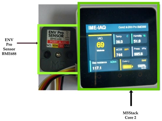
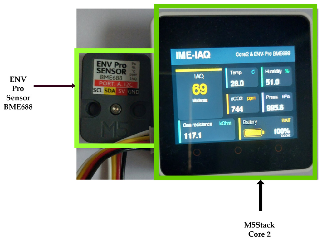
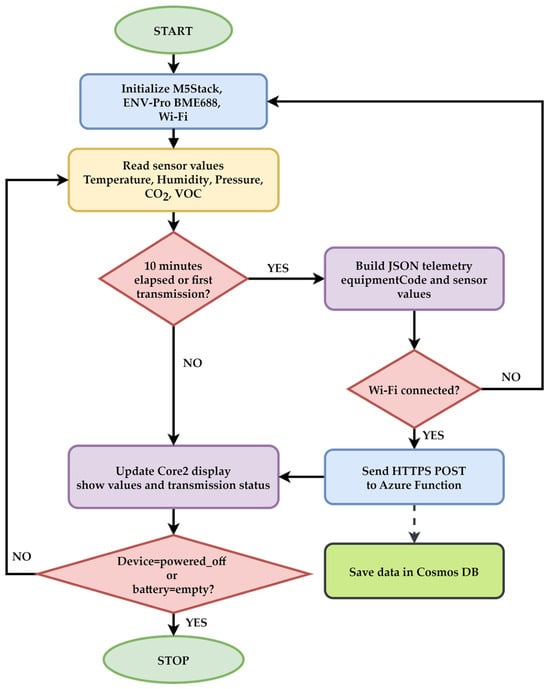
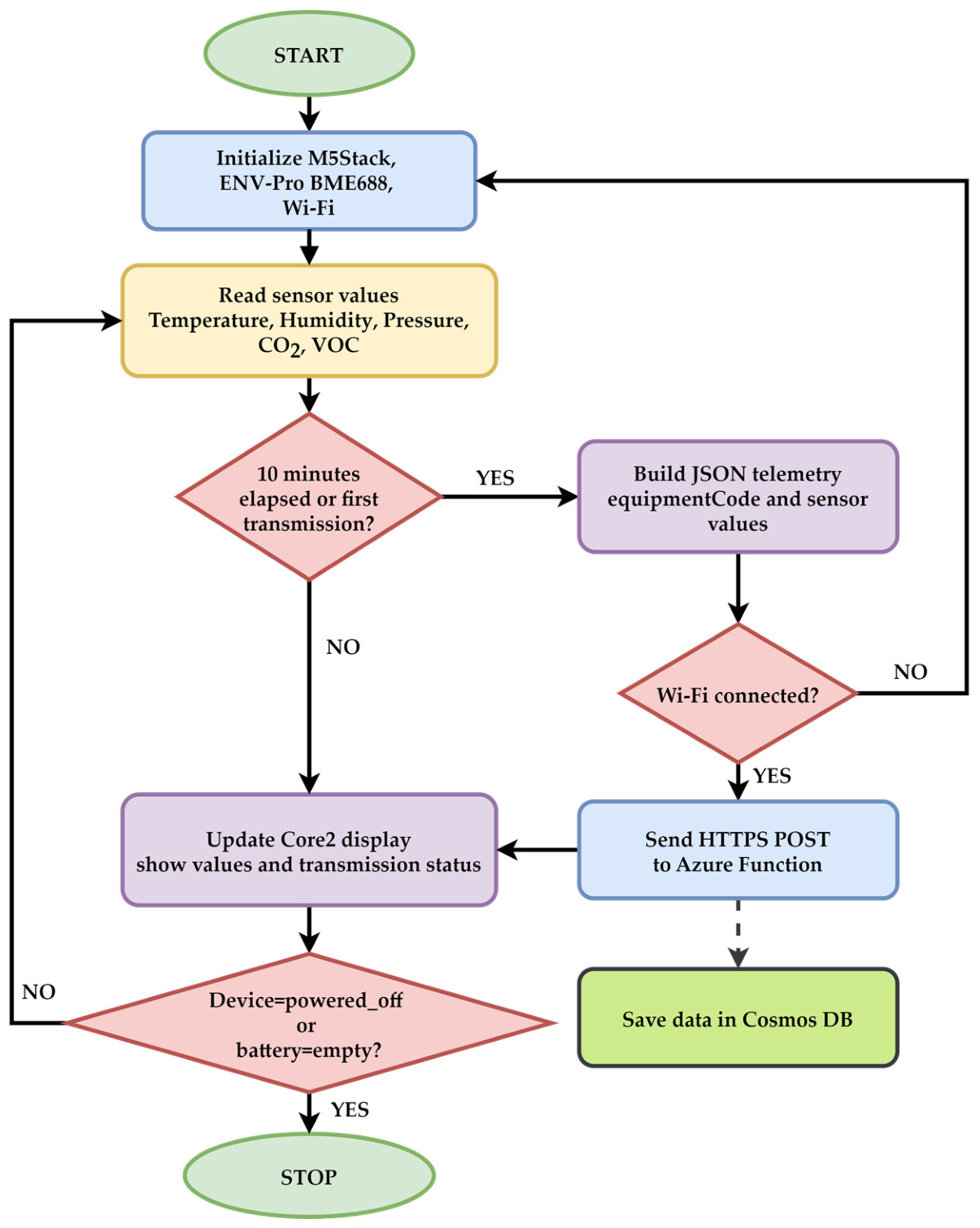
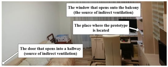
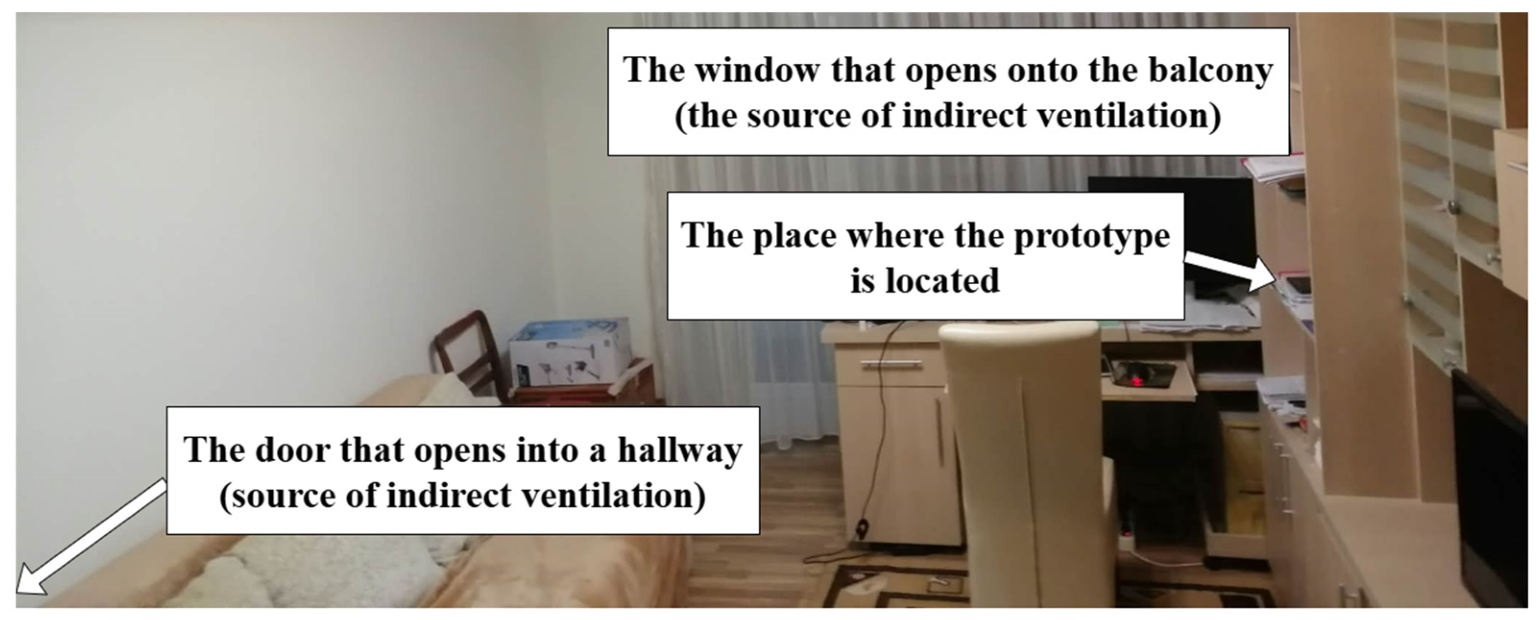
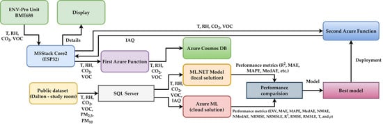
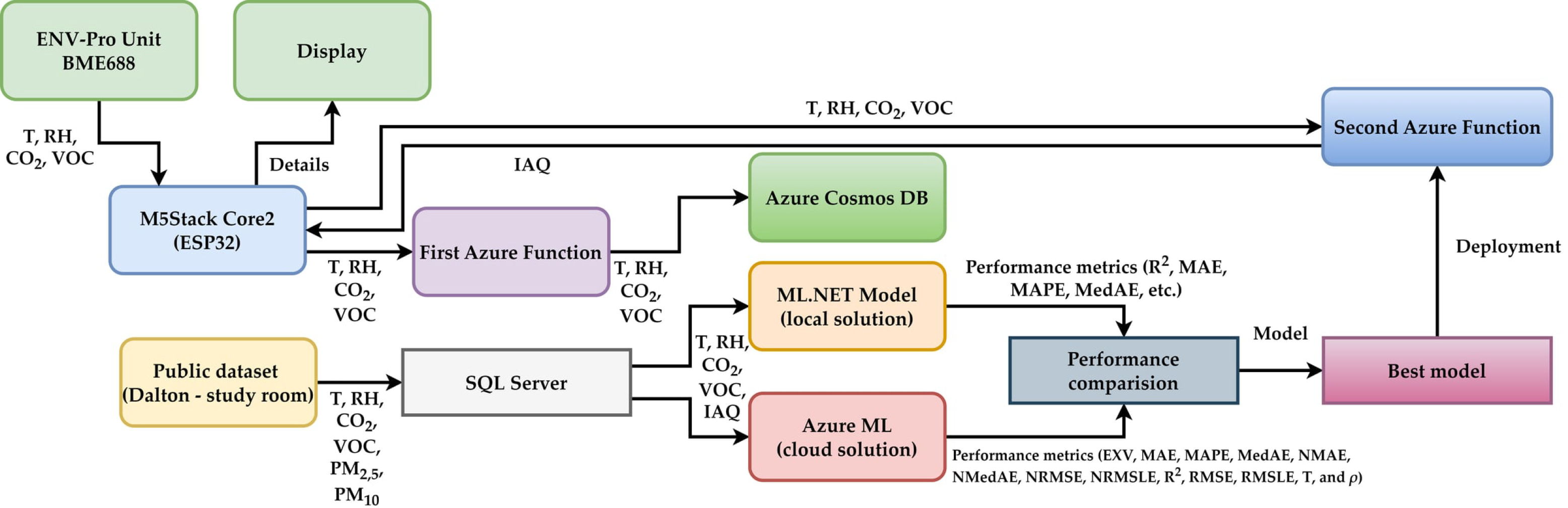
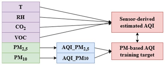
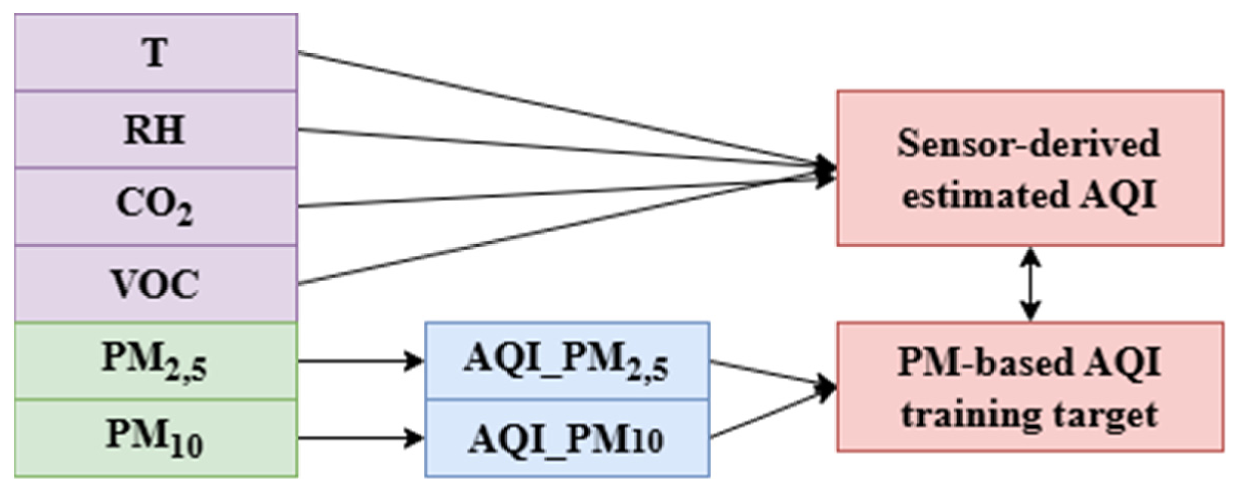
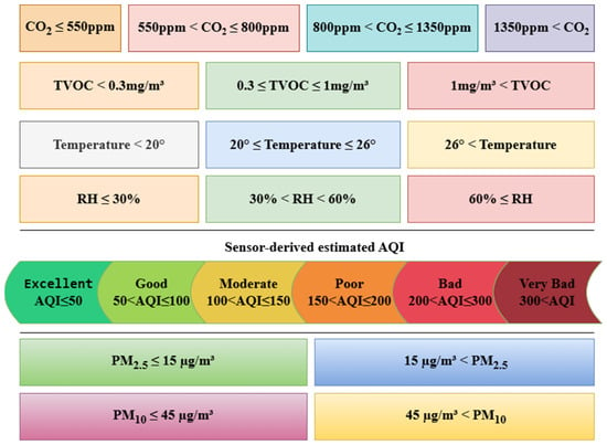
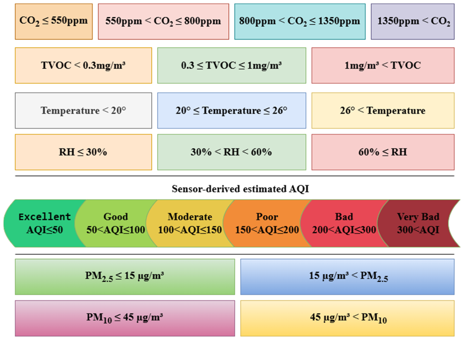
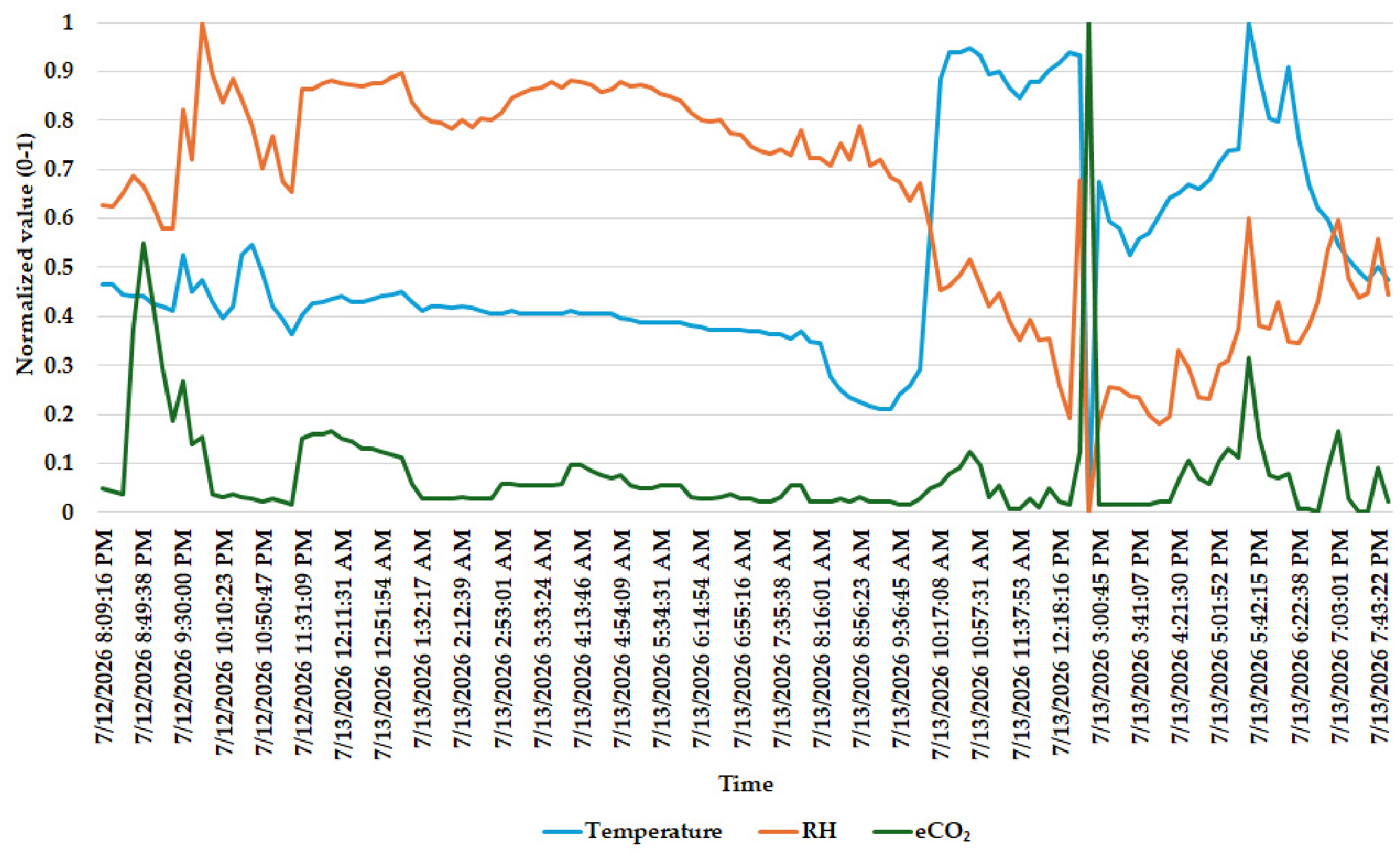
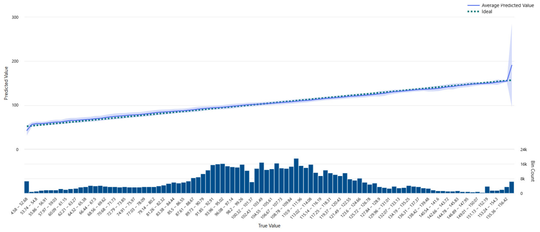
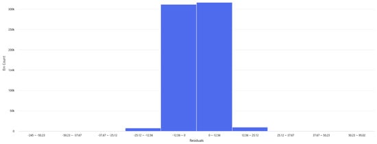
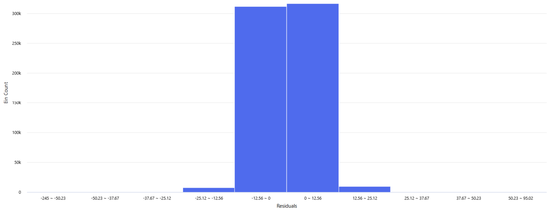
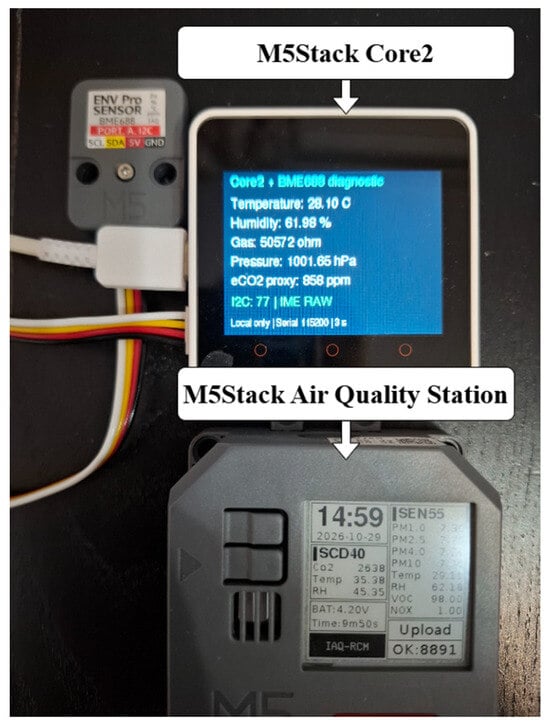
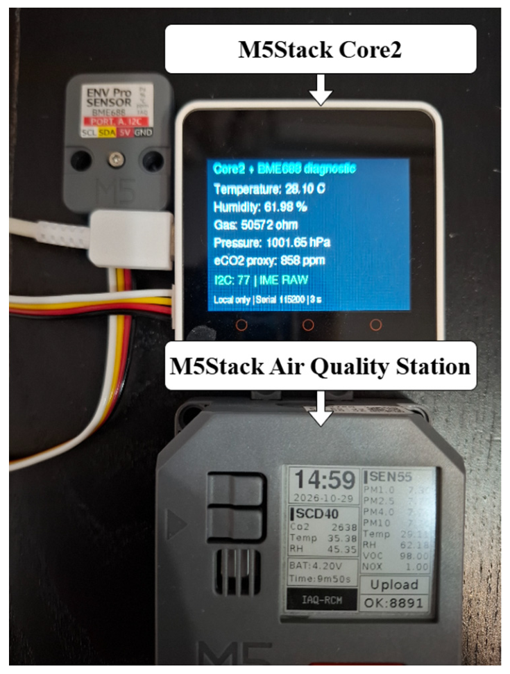

Disclaimer/Publisher’s Note: The statements, opinions and data contained in all publications are solely those of the individual author(s) and contributor(s) and not of MDPI and/or the editor(s). MDPI and/or the editor(s) disclaim responsibility for any injury to people or property resulting from any ideas, methods, instructions or products referred to in the content. |
© 2026 by the authors. Licensee MDPI, Basel, Switzerland. This article is an open access article distributed under the terms and conditions of the Creative Commons Attribution (CC BY) license.