


Abstract
We propose a joint response-based procedure to determine when one constant compression coefficient is sufficient for both pile drag increment and head settlement. Ordered compression-strain bounds are propagated through a finite-stiffness pile with fixed monotone shaft and toe laws; acceptable coefficient intervals are then intersected. Of 500 synthetic configurations, 339 pass a physical screen (upper strain at most 5% and soil–pile movement at most 0.3 m); in this subset, 335 admit a constant matching their prescribed nonlinear reference within 10%, whereas only 35 satisfy the conservative response-box test. Nine published compression curves provide approximation and withheld-stress checks. Explicit smooth whole-curve witnesses and curvature-constrained enclosures show which conclusions require additional shape information. A Bangkok stage-transfer reconstruction fails; a settlement-independent force-capacity bound identifies incompatibility of the frozen fitted transfer model with later observations. A worked single-pile example with explicit effective stress shows that groundwater lowering can change the decision and separates approximation accuracy from conservative design demands. The procedure supports conditional simplification decisions while making missing compression or transfer information explicit.
1. Introduction
Pile-supported buildings on compressible ground require separate checks of structural force demand and settlement. Relative soil–pile movement mobilizes negative skin friction; pile stiffness and toe restraint then affect the additional drag force and head movement. Unified pile-design guidance distinguishes these response questions [1,2,3], and centrifuge observations show that reduced drag can coexist with increased settlement [4]. Building settlement, piled-raft design, and monitored load sharing also require more than one response measure [5,6,7,8]. The present study addresses a single-pile component of that assessment, rather than complete building-foundation performance.
Construction stage and transfer conditions matter. Building and long-term pile monitoring illustrate changing settlement and axial-force response [9,10,11]; experiments and analyses identify effects of group arrangement, interfaces, and construction-stage interpretation [12,13,14,15]. Established approaches already combine consolidation, relative movement, and nonlinear transfer, including finite-strain, drainage, loading-history, and creep effects [16,17,18,19,20,21,22,23,24,25]. Our question is narrower: within a specified forward model and loading stage, can the same constant compression coefficient meet tolerances for drag increment and pile-head settlement?
Compression behaviour can depend on structure, stress window, disturbance, and loading branch [26,27,28,29,30]. A curved loading relationship is not interchangeable with nonlinear permeability, evolving geometry, unloading–reloading, or creep [31,32,33,34,35]. These distinctions are important when interpreting an endpoint compression comparison: replacing a constant coefficient does not supply missing hydraulic or history variables.
The candidate nonlinear family follows the square-root joining expression used in the Simplified Silty Sand model [36] and later oedometer and hardening applications [37,38]. Here, AJOP means Arc Joint via Optimum Parameters and denotes only the generalized one-dimensional compression family defined below. The lineage does not make mean stress, vertical effective stress, and hardening pressure interchangeable. A related storage study is a non-peer-reviewed preprint and is not independent foundation validation [39]; interpretation of fitted transition stresses also depends on available stress support [40].
Published Manitoba, Randers, and Haihe programmes provide nine compression curves with distinct reporting conditions [41,42,43]. Their data support reanalysis of fit, shape, and stress-window prediction; they do not form nine independent field validations. Monitoring-based updating provides a complementary route to settlement assessment [44]. We therefore distinguish computational verification from evidence for an intended engineering use [45].
The contribution is a common-coefficient decision based on both coupled outputs under fixed transfer assumptions. Synthetic configurations reveal head-load masking and the distinction between matching a particular reference and meeting conservative response bounds. Laboratory reanalysis examines compression information; Bangkok monitoring [46] challenges cross-stage transfer. Headline synthetic counts are given for a physically screened subset, and a worked endpoint example with explicit effective stress includes groundwater lowering. Additional diagnostics and reproducible numerical records are retained in Supplementary Material S1.
2. Materials and Methods
2.1. Evidence Structure and Scope
Table 1 organizes the core evidence around the decision sequence. Published Manitoba and Randers programmes supply three reconstructed laboratory curves with 25 loading markers [41,42]. Six tabulated Haihe curves add 66 positive-pressure entries [43]. The nine curves span three programmes with different reporting conditions. Five hundred selected synthetic configurations test the coupled response decision, and two Bangkok piles provide a monitored stage-transfer check [46]. Extended analyses of Tokyo monitoring [47], open static-load-test data [48,49,50], a sand–aluminum interface experiment [51], composite-foundation and groundwater-rise studies [52,53], and the Cai Mep building history [54] are retained in Supplementary Material S1. They document applicability and provenance rather than enlarge the core prediction sample.
Table 1.
Evidence units and the questions they can support.
Figure-reading tolerances are deterministic analyst-selected reconstruction bounds. Instrument accuracy, specimen variability, and statistical confidence require different evidence. The numerical audit reuses the recorded observations to verify calculation and optimization. Supplementary Material S1 separates source measurements, reconstructed coordinates, assumptions, and computed outputs, and it supplies a portable headline-reproduction command.
Four qualifications apply throughout this paper. (i) Synthetic counts describe a prescribed benchmark domain, not frequencies of successful field designs. (ii) Reading tolerances on digitized figures are analyst-selected bounds, not instrument accuracy or confidence intervals. (iii) Fitted transition stresses and asymptotes describe the observed stress window and are not identified physical parameters. (iv) The laboratory and field checks test parts of the chain separately; no independent field case yet tests the complete prediction from compression to drag and settlement (Section 4.4).
Soil Context and Interpretation of the Driving Stress
The Manitoba source describes heterogeneous overconsolidated glacial clay till, including sand and gravel lenses, with water contents of approximately 15–22% and plasticity indices of 18–28 [41]. Its 11 m and 23 m compression observations are treated as specimen-specific curves. Randers comprises organic marine gyttja: the reported organic content is 7.5–9.1%, liquid limit 101–111%, plastic limit 42–52%, and water content approximately 70–150%; reported OCR is about 2.1 at 2.6 m and 1.7 at 4.5 m [42]. The sand below the soft layer is slightly artesian, and the old fill has a separate perched water table. These programme ranges are not assigned as measurements on every reconstructed specimen. In particular, the strain-only Randers ordinate is not converted into an unreported void ratio.
The Bangkok experiment applied a 2 m embankment and monitored pore pressures and movements over approximately 9 months [46]. The source describes normally or lightly overconsolidated upper clay, liquid limits of 70–100%, plastic limits of 25–40%, and a water table approximately 1.5–2 m below ground. Regional pumping and piezometric drawdown are relevant background mechanisms, but the present reconstruction does not identify their contribution to the observed stage difference. The six Haihe specimens retain the nominal-pressure qualification below; missing drainage, pore-pressure, duration, OCR, and structure information is not inferred from the quality of a curve fit.
For a field application, the driving variable is σ′(z,t) = σv(z,t) − u(z,t). Fill changes total stress; groundwater lowering changes pore pressure; consolidation dissipates excess pore pressure. The supplied synthetic stress endpoints prescribe the net change and do not solve for u(z,t), drainage, or the time to reach that change. Field use therefore requires externally justified endpoints or a separate hydrogeological/consolidation analysis. Section Worked Endpoint Example for a Pile Carrying a Building Load evaluates σ′ = σv − u explicitly for a surcharge, a groundwater-lowering, and a combined endpoint. The Bangkok diagnostic conditions on observed soil settlement rather than predicting it from a compression law.
2.2. Compression Variables and the AJOP Candidate Family
Let z increase downward, let vertical engineering compression be positive, and let σ0′(z) and σ1′(z) denote the initial and final effective vertical stresses on a specified monotone loading path. For void ratio e and its local natural-logarithmic slope λt, the strain relative to the initial state is
Here, the prime denotes effective stress, not differentiation. When the published ordinate is engineering strain F relative to the original laboratory height, a new increment beginning at F0 requires a different denominator. A slope reported per base-10 logarithm must also be converted consistently:
Cε,10 denotes a strain slope per log10 stress at the same reference state. For a void-ratio compression index Cc, λ = Cc/ln 10. A strain slope is not a void-ratio slope unless the reference void ratio is known. This distinction is essential for Randers, whose plotted ordinate is strain; no unreported void ratio is assigned to that specimen.
The square-root transition appears in Equation (3) of the Simplified Silty Sand model [36], where the stress variable is mean effective stress. Phonchamni et al. subsequently applied an AJOP formulation to oedometer-based consolidation settlement [37]. The present centered generalized family adds a nonnegative low-stress baseline slope. With u = ln(σ′/pr), λ∞ ≥ λ0 ≥ 0, and θ > 0,
For a positive SSS slope parameter α and θSSS > 0, the earlier square-root expression is recovered algebraically with λ0 = 0, λ∞ = 2α, θ = θSSS/α2, and er = Γ − √θSSS [36]. The curvature parameters have different scaling; the mean-effective-stress and vertical-effective-stress coordinates are not physically interchangeable. This lineage statement does not assert global priority for square-root smoothing functions.
The square-root transition has a nondecreasing logarithmic compression slope, a restriction tested against each observed stress window. The algebraic form of the published AJOP-T map is recovered with λ0 = 0, λ∞ = 2ac, and er = Γ − ac√θ [38]. AJOP-T uses a hardening-pressure coordinate; Equation (3) applies the generalized shape to a one-dimensional vertical-stress loading path. AJOP in the figures denotes this defined family. The transition stress pr is a fitting coordinate; identifying it with preconsolidation stress or interpreting fitted asymptotes physically requires additional evidence. Controlled tests show that the included stress range affects interpreted preconsolidation pressure [40]. Bound-hitting optima are reported explicitly and are not treated as proof that the parameters are physically identified. Figure 1 illustrates the curve geometry and limiting slopes.
Figure 1.
Generalized AJOP geometry: (a) Equation (3), limiting asymptotes and slope triangles; (b) the analytical tangent from Equation (4). Triangle labels are normalized to a unit horizontal increment; triangle sizes are schematic. Illustrative parameters are λ0 = 0.02, λ∞ = 0.15, er = 0.90, and θ = 0.25. The shaded interval −√θ ≤ u ≤ √θ indicates transition scale, not a measured yield range. Parameters are illustrative, not fitted observations.
2.3. Reconstruction, Fitting, and Independent Numerical Audit
The Manitoba reconstruction uses vector marker coordinates from the published compression plot, with eight initial-loading markers per specimen. Six unloading/reloading markers per specimen are retained separately. The initial-loading range is approximately 16.5–2936 kPa. Assigned reading bounds are ±0.0015 in void ratio and ±0.01 in log10 stress. The Randers reconstruction uses nine initial-loading marker centres over approximately 4.97–1190 kPa, with bounds of ±0.003 strain and ±0.015 in log10 stress. Branch connectivity and ordinate units are preserved in the supplied extraction records.
For fitting, x = ln(σ′/kPa) and compression-positive F is −e for Manitoba and laboratory engineering strain for Randers. The fitted expression is algebraically equivalent to Equation (3), with a free ordinate at a reference x0:
Here, q = ln(pr/kPa), Δc ≥ 0, and c∞ = c0 + Δc. The original fit minimizes unweighted vertical squared residuals at the reconstructed stresses using 16 starts. Parameter bounds for (a, c0, Δc, q, ln θ) are (−2, 0, 0, −12, −14) to (2, 2, 4, 22, 16). These bounds define a numerical search domain, not a physical prior. Constant and bilinear compression fits provide reference families with two and four parameters; AJOP has five. No information criterion or statistical significance test is inferred from these small, digitized samples.
An independent implementation rationalizes the square-root difference and separates two nonlinear parameters from three bounded linear coefficients. Differential evolution searches using three seeds, followed by least-squares polishing, check the original least-squares objective. A separate minimax search uses linear programming for the largest absolute ordinate residual and two nonlinear search seeds. Agreement between implementations is numerical verification; neither search proves global optimality. Horizontal reading uncertainty is displayed and used in the secant shape test, but the fitting objectives hold reconstructed stresses fixed. Thus, the fits are not errors-in-variables likelihood analyses.
A retrospective Randers stress-window holdout fits the first seven markers and predicts the last two. These are withheld stress levels from one specimen, not independent specimens or blind field validation. All four original parameterizations are retained: Manitoba 11 m, Manitoba 23 m, the full Randers curve, and its seven-point fit. Frozen parameters and numerical diagnostics remain in Supplementary Material S1; the main figures distinguish licensed source observations from computed analyses.
2.4. Finite-Stiffness Pile Model and Conditional Ordering
For a pile of length L, let N(z) be positive compressive axial force, w(z) downward pile displacement, S(z) free-field soil settlement, p(z) perimeter, and EA(z) axial rigidity. The shaft shear stress T is positive when the soil moves downward relative to the pile; pT is force per unit pile length. The base datum is S(L); soil settlement at depth z equals this base settlement, plus the integrated strain below z. The equilibrium and compatibility problem is
The applied head load P, rigidity, geometry, shaft law T, toe law B, and settlement datum S(L) are held fixed within each compression comparison. T and B are memoryless, single-valued, monotone increasing functions of their relative movements; the demonstrated smooth model uses a tanh shaft law and a linear toe spring. Comparisons involving a changed effective-stress capacity, interface stiffness, residual state, or loading history are outside this fixed-law statement. Existence and sufficient regularity of the compared solutions are assumed, with strictly positive tangent response for the elementary comparison proof; limiting plateau cases require a suitable well-posed limit.
If ε−(z) ≤ ε(z) ≤ ε+(z), and settlement is integrated from the same base datum, the finite-stiffness comparison gives pointwise force and pile-displacement ordering:
Appendix B proves Equation (7) using force differences and a negative-part test. The required ordering is in strain, not merely in settlement values; all compared profiles use a common base datum and unchanged transfer laws.
Equation (7) bounds response values, not their depth locations. Let r(z) = S(z) − w(z). Where perimeter is positive and the strictly increasing shaft law has T(z,0) = 0, Equation (6) gives N′(z) = 0 if and only if r(z) = 0. A crossing from r > 0 to r < 0 is a local force maximum; the reverse crossing is a minimum. A zero without a sign change need not be an extremum. Compare all candidate extrema with head and toe forces to obtain the global maximum. In the usual single-crossing case, the positive-to-negative zero-slip neutral plane is the force maximum. Multiple crossings, zero-capacity zones, and boundary maxima require separate checks. The ordering theorem does not order neutral-plane depths; adding self-weight or residual forces also changes the corresponding equilibrium check.
The response targets are the drag increment D and pile-head settlement W, not two definitions of the same quantity:
Testing total maximum force instead of D can conceal substantial relative drag error when P is large. Each response is therefore reported separately. The numerical examples use positive head settlement and compression loading. Their 10% tolerance is an illustrative analyst choice and is not attributed to a design code. Figure 2 shows the model and its synthetic base discretization.
Figure 2.
Pile interaction and the synthetic base mesh: (a) prescribed soil movement, axial pile response, and toe restraint; (b) 201 uniformly spaced nodes and 200 axial segments; (c) interior nodal equilibrium with trapezoidal shaft weights. Displacements are nodal and axial forces are segment quantities. The Bangkok diagnostic uses a separate mesh. Schematics are not to scale.
2.5. Joint Adequacy of One Constant Coefficient
Consider an unknown nonnegative response Q in an outer interval [A, B], with 0 ≤ A ≤ B, and a constant-law prediction Qc. For 0 ≤ τ < 1 and an absolute allowance δ ≥ 0, requiring |Qc − Q| ≤ τQ + δ for every Q in the interval is equivalent to
Monotone response to the constant coefficient converts this target interval into a feasible coefficient interval for each output. One coefficient is adequate for drag and settlement together only if those intervals intersect. If several transfer scenarios are enumerated, the same coefficient must lie in the intersection over both outputs and all those scenarios:
Within each scenario, the reference and constant models use identical transfer parameters. For the void–ratio examples, the scalar surrogate has εc(z) = λc ln[σ1′(z)/σ0′(z)]/[1 + e0(z)] with fixed local initial states. The inverse search retains the rightmost feasible endpoint on zero-drag plateaux. The inequality |Qc − Q| ≤ τQ with δ = 0 requires zero predicted drag when Q = 0; no division by zero is used. Practical applications should specify a meaningful absolute allowance near zero. All quoted synthetic counts use strict relative tolerance so that the numerical rule is fully reproducible.
A nonempty common interval certifies the stated tolerance for the declared response box within the model and numerical accuracy. An empty intersection for a conservative outer box means that this information cannot certify the simplification. For a prescribed nonlinear reference, disjoint intervals instead demonstrate incompatibility of the constant-law class with that reference. Section 4.1 gives a dimensionless form and the corresponding action in each case. The interval algebra is elementary; the engineering decision requires the same coefficient to satisfy both coupled outputs and every declared transfer scenario.
2.6. Laboratory Point Envelopes and Numerical Experiments
For a monotone laboratory strain curve F, point-reading rectangles give lower and upper functions Fl and Fu within the measured stress support. Incremental strain relative to the initial state is bounded by
The construction requires ordered, admissible observation boxes, and 0 ≤ Fl ≤ Fu < 1. It does not extrapolate beyond measured support. A second construction adds piecewise-linear interpolation in log stress between uncertain nodes. The latter is an additional shape assumption, not information supplied by more observations. Pointwise extreme strains may not be jointly realizable by one common laboratory curve; the resulting response box can consequently be conservative.
The numerical collection contains 500 selected parameter sets, with sampling domain and seed reported in Table A2. The base mesh has 201 nodes; selected conclusions are checked on finer meshes. Transfer tests enumerate 27 combinations of shaft-capacity multipliers (0.5, 1, 1.5), mobilization-slip multipliers (0.5, 1, 2), and toe-stiffness multipliers (0.5, 1, 2). These deliberate stress tests describe the enumerated scenarios, not extrema over the continuous parameter box.
Five existing synthetic pile configurations are also subjected to the Randers laboratory envelopes. They are not reconstructions of the Randers pile geometry. In these examples, the surrogate coefficient c multiplies ln(σ1′/σ0′) in engineering strain; it is not relabelled Cc. Fixed depth, stress profiles, and geometry are retained, so cases with large, calculated strains illustrate the algorithm rather than validate a small-strain physical approximation.
AJOP is used in the synthetic collection because its prescribed slope bounds, transition location, and width give a controllable nonlinear benchmark. The parameter draws in Table A2 are independent of the laboratory calibrations in Table A1. The synthetic reference is known by construction within this model; it is not selected as a validated soil law. The interval procedure also accepts laboratory point envelopes and does not require an AJOP reference. Each synthetic case uses a homogeneous slope function with locally anchored initial states, rather than imposing one global e(σ′) curve at all depths. Frozen inputs, mesh checks, and executable analyses are supplied in Supplementary Material S1.
2.7. Tabulated Haihe Curves and Blocked Prediction
The two-page supplement of Su et al. contains specimens D2-18–D2-23, each with 11 positive nominal pressures of 50, 100, 200, 300, 400, 500, 600, 800, 1000, 1200, and 1600 kPa and void ratios printed to three decimal places [43]. All 66 entries were transcribed and independently checked against both source pages. Duplicate zero-pressure entries are retained once as reference states and excluded from logarithmic fitting. The D2-20 table has a different printed identifier from its adjacent graph, and D2-22 has a depth typographical ambiguity; both are recorded in Supplementary Material S1, and neither affects fitting. Test duration, drainage completion, specimen height, and pore pressure are not reported in the inspected source material. Consequently, p is treated as nominal applied pressure, not independently verified equilibrium effective stress.
The same generalized algebraic family is fitted to void ratio against x = ln(p/kPa), anchored at x0 = ln 50. The parameter vector is (a, c0, Δc, q, ln θ), where a is the fitted void ratio at 50 kPa. Bounds remain (−2, 0, 0, −12, −14) to (2, 2, 4, 22, 16). Each least-squares search uses 32 starts and is checked with a separate two-dimensional variable-projection search: bounded linear coefficients are solved at each (q, ln θ), which are searched by differential evolution. Supplementary Material S1 gives seeds, solver tolerances, all parameter sets, and predictions. These checks establish numerical agreement within the searched domain, not global optimality or physical identification of asymptotes.
Comparators are a two-parameter constant logarithmic slope and a continuous four-parameter bilinear law with nonnegative low slope and nonnegative slope increment. The bilinear breakpoint is searched within the calibration stress range. Full-window fits use 11 points. A separate retrospective blocked test fits only the first nine points, 50–1000 kPa, and evaluates the two withheld observations at 1200 and 1600 kPa. No withheld ordinate enters an optimizer. Errors are unweighted void-ratio RMSE and maximum absolute residual; the six pairs of held-out points are not 12 independent specimens. The comparator restrictions and parameter counts are reported because improved calibration with added flexibility is not, on its own, validation [45].
A separate shape test minimizes the largest ordinate residual over every nonincreasing concave sequence in log pressure, using linear programming. Successive void–ratio secants must therefore be nonincreasing. Because every admissible AJOP curve has this property, the relaxed optimum is a lower bound on the AJOP minimax residual, independent of the nonlinear optimizer. Three-point chord defects provide a separate analytical check of the active lower bounds. The bound is compared with ±0.0005 only as an assumed nearest-rounding band for the printed values. That band is neither measurement uncertainty nor a confidence interval. A lower bound exceeding it rejects exact compatibility with the declared shape and rounding assumptions; it does not reject approximate use over a narrower pressure interval.
2.8. Additional Admissibility and Sensitivity Checks
The 500 archived inputs are retained. Final void ratio e1 = e0 − (1 + e0)ε, maximum strain, and relative soil–pile movement are audited nodewise. Headline counts are reported for a physically screened subset in which the upper-envelope strain is at most 5% at every depth and the largest upper-envelope relative soil–pile movement is at most 0.3 m. These limits are analyst screens that exclude large-strain and metre-scale slip cases, not validated physical limits; other strain and movement limits are reported as sensitivity checks (Section 3.6), and the full collection is retained in Supplementary Material S1.
Two distinct whole-curve tests address the information class. First, explicit monotone C2 curves pass through every Randers marker centre using quintic smooth-step transitions. They provide constructive response witnesses, not estimates of the most likely soil behaviour. Second, let x = log10(σ′/kPa) and impose an explicitly assumed bound |F″(x)| ≤ K, or equivalently a K-Lipschitz first derivative. The linear-interpolation error bound K(x − a)(b − x)/2 is combined with all uncertain marker rectangles and monotonicity to enclose F throughout the stress window. Rebased strain bounds are propagated through Equation (7). Unlike finite curve sampling, these are enclosing bounds for the stated class; the equilibrium solutions and depth integration remain numerical. A monotone natural C2 spline through the marker centres establishes nonemptiness of the K = 0.75 class. No measured curvature limit or experimental probability distribution is inferred. Supplementary Material S1 gives the proof, witness coefficients, finite-grid consistency screen, and 201/801/1601-node checks.
For Bangkok, the observed settlement profile is supplied directly, bypassing the compression law. In addition to controlled parameter perturbations, equilibrium is used to derive settlement-independent shaft-capacity bounds. Both continuous and discrete representations, force-reading, and depth-reading allowances are checked. A broader finite scenario scan releases the original deep-settlement relation and samples the separate deep reading intervals and shallow ordinate corners. This is not an exhaustive uncertainty propagation or causal variance decomposition.
3. Results
3.1. What the Laboratory Fits Establish
Figure 3 compares the Manitoba compression observations with our full-window AJOP fits and residuals; Table 2 also reports the Randers errors.
Figure 3.
Manitoba loading data (blue) and full-window AJOP fits (red): (a,b) 11 and 23 m; (c,d) fit-minus-data residuals. Bars: assigned digitization halfwidths of ±0.0015 in e and ±0.01 in log10 stress; residual shading: ±0.0015 in e. Allowances are not confidence intervals. Data reconstructed and reanalysed from Chalajour and Blatz [41] (CC BY 4.0); graphics generated here.
Table 2.
AJOP fitting errors: least squares (LS), root-mean-square error (RMSE), and the distinct minimax objective. Randers errors are percentage points (pp) of engineering strain.
An independent least-squares implementation reproduces the original objectives to within 5 × 10⁻¹⁴ relative difference in summed squared residuals. The Manitoba 11 m fit lies within its selected ordinate-reading band; Manitoba 23 m and the full Randers fit exceed theirs. Both Manitoba fits approach the zero lower-slope bound, and the full Randers fit reaches the lower transition-width bound. These solutions support assessment of approximation over the observed window. They do not establish physical identification of the unobserved asymptotes or transition parameters.
Least-squares and minimax fitting answer different questions. The seven-point Randers least-squares maximum residual slightly exceeds ±0.003 strain, while the independently searched minimax fit lies inside that ordinate band at the fixed reconstructed stresses. Thus, a least-squares miss is not proof that no AJOP curve can fit within the band. For Manitoba 23 m and full Randers, the searched minimax residuals remain above their selected bands. These optimization results remain numerical searches, not global nonexistence proofs.
The seven-point Randers fit misses its two withheld high-stress markers by up to 4.631 percentage points of strain (Figure 4). The minimax calibration gives a comparable held-out maximum of 4.604 percentage points. The additional flexibility of the fit therefore does not remove the observed stress-window extrapolation problem. The training/holdout split tests transfer along one specimen curve and cannot be counted as a new field or laboratory experiment.
Figure 4.
Randers stress-window prediction: (a) AJOP strain from a seven-point fit and its continuation to withheld stresses; (b) predicted-minus-observed strain (percentage points). Teal denotes calibration steps 1–7; orange denotes withheld levels 8–9. Predictions and errors were calculated here from reconstructed observations in Kania et al. [42]. This retrospective same-specimen check is not independent-specimen validation.
The shape check is independent of optimization. Consecutive Randers secant slopes over approximately 79–295 and 295–1190 kPa are 0.30528 and 0.23430 strain per log10 stress. Allowing the stated horizontal and vertical reading boxes gives intervals [0.28010, 0.33325] and [0.21378, 0.25695]. Their strict separation excludes a globally nondecreasing logarithmic slope over this measured window at the stated reading level. It does not exclude approximation over a narrower field stress path.
The separate Manitoba unloading/reloading observations show why a single memoryless function of stress cannot be used for both branches. These points were never included in the initial-loading objective. A field loading path involving unloading, reloading, or creep needs an appropriate state or branch description before the compression envelope is propagated.
Figure 5 compares calculated adjacent-observation secants with fitted analytical tangent slopes, using the same median adjacent secant to normalize both in each panel. The secant points are not direct tangent measurements, and normalization does not identify observed asymptotic bounds.
Figure 5.
Normalized logarithmic slopes for (a) Manitoba 11 m, (b) Manitoba 23 m, and (c) Randers 2.6 m. Points are adjacent-observation secants at geometric-mean stresses; curves are analytical AJOP tangents. Both are divided by the median positive adjacent natural-logarithmic secant in each panel. Secants are calculated, not measured tangents; normalization does not establish asymptotic bounds. Observations: Chalajour and Blatz [41] (CC BY 4.0, https://creativecommons.org/licenses/by/4.0/ (accessed on 18 October 2026)) and Kania et al. [42]. Calculations and graphics were generated here.
3.2. Joint Force and Settlement Decisions
Head-load masking changes outer-envelope certification. In the 339 screened cases at the same joint 10% tolerance, 57 certify the total-maximum-force and settlement envelopes, whereas 35 certify the drag-increment and settlement envelopes. All 35 drag-based certificates are contained in the total-force set. The difference is 22 cases, or 38.6% of the 57 total-force certificates (in the full collection of 500: 105, 76, and 29).
For a positive reference drag D, define relative prediction errors EΣ for total maximum force P + D and ED for drag alone. With the same head load P in both compared solutions, the exact relation is
Equivalently, a relative total-force allowance τ permits |Dc − D| ≤ τD + τP: the head load supplies an additional absolute allowance τP for drag error. This inequality also avoids division by zero. The 22 cases lose certification against the outer response box when the output definition changes; all 22 still admit a constant matching their particular synthetic AJOP reference within 10%. They must therefore not be counted as 22 demonstrated prediction failures. In the screened subset, 335 cases match their prescribed synthetic reference (496 of 500 in the full collection). Thirty-one reference responses and 58 lower-envelope responses have zero drag; all of them lie in the screened subset. Table 3 separates these decisions.
Table 3.
Selected numerical decisions at 10% relative tolerance. Counts refer to the 339 physically screened cases; Cases 31 and 477 lie outside the screen and illustrate the algorithm only.
The discrepancy between 335 reference matches and 35 outer-bound acceptances is primarily an information-width effect. Of the 304 screened configurations that fail the outer drag–settlement test, 32 fail the scalar drag-width screen only, 9 fail the settlement-width screen only, and 263 fail both. Thus, none of these 304 failures requires disjoint coefficient intervals after both scalar screens pass. This breakdown shows why failure to meet an outer response box cannot be equated with failure against a particular compression curve.
Figure 6 contrasts the three numerical decisions and shows the Case 100 coefficient intervals. Case 31 has a slope ratio of 7.27, yet its drag bounds are 273.80–303.67 kN and its head-settlement bounds are 2.889–2.968 mm. A constant λc ≈ 0.07038 gives a worst joint error of 5.17%, with an approximate 10% feasible interval [0.04113, 0.19818]. A large slope ratio alone therefore does not imply unacceptable pile-response error. Case 31 lies outside the physical screen (upper strain 10.5%, movement 0.62 m), so it illustrates the algorithm rather than a screened design case.
Figure 6.
Synthetic joint-response tests at 10% tolerance: (a) counts admitting reference matching, total-force-plus-settlement outer-envelope acceptance, or drag-plus-settlement outer-envelope acceptance, for the 339 physically screened cases (filled) and all 500 cases (hatched); (b) disjoint Case 100 coefficient intervals for reference drag and settlement on 1601 nodes. W denotes pile-head settlement.
Case 100 gives a contrasting reference comparison. On 1601 nodes, its prescribed nonlinear reference gives drag 163.59 kN and head settlement 139.35 mm. The 10% coefficient intervals are approximately [0.01309, 0.01392] for drag and [0.01575, 0.02159] for settlement, so no common coefficient exists. The minimum joint relative error is 16.12% at λc ≈ 0.014174. Mesh refinement from 201 to 1601 nodes changes that error by less than 0.006 percentage points; detailed values are retained in Supplementary Material S1. Its declared slope interval is approximately 0.004710–0.02925.
Case 9 separates masking from lack of information. With head load 702.1873 kN, its total-force/settlement certificate passes, but the best drag/settlement outer-envelope error is 17.20%. A constant nevertheless matches its prescribed synthetic AJOP response with about 0.1101% joint error. Thus, the outer box is insufficient for certification even though the particular synthetic curve can be approximated.
A separate location check illustrates why Equation (7) is not a neutral-plane theorem. In Case 372 on 1601 nodes, the low-bound, reference, and high-bound crossings are approximately 7.30, 13.78, and 13.12 m. The reference crossing is about 0.66 m deeper than the high-bound crossing even though peak forces remain ordered at 111.09, 168.35, and 495.39 kN. Full numerical values remain in Supplementary Material S1.
3.3. Sensitivity to Transfer Assumptions and Laboratory Information
For Case 31, 26 of the 27 selected transfer scenarios individually admit a joint 10% outer-envelope certificate, but there is no single coefficient certifying all 27. A constant matching the synthetic AJOP reference response across all 27 still exists, approximately over [0.07120, 0.29920]. The nuisance-only AJOP response width is 10.35 times the compression-only drag width and 40.49 times the compression-only settlement width. Case 477, which also lies outside the physical screen (upper strain 24%, movement 1.56 m), retains a common coefficient interval, approximately [0.04140624, 0.15862844], across all 27 scenarios; its corresponding width ratios are 20.35 and 69.02. These comparisons show when more compression detail alone cannot remove the dominant response spread.
The Randers experiment reuses the Case 31 configuration from Section 3.2, which lies outside the physical screen, but replaces synthetic slope bounds with laboratory marker envelopes, giving different drag bounds. Monotonicity alone gives drag bounds of 0–307.71 kN from five markers and 0–306.90 kN from all nine; neither certifies the strict 10% requirement. Piecewise linearity in log stress between the same nine uncertain nodes gives 301.06–305.58 kN and head settlement 2.962–2.972 mm. Acceptance is conditional on that added shape restriction; no measurements were added, and monotonicity alone remains uncertified.
The zero lower-strain corner in the monotonicity-only construction need not correspond to one jointly realizable laboratory curve. This explains part of the conservatism and reinforces the distinction between lack of certification and actual surrogate failure. Refining the step-envelope calculation through 6401 nodes leaves the no-certificate conclusion unchanged; the upper drag converges to approximately 306.894 kN. These are finite-grid numerical bounds, not interval-arithmetic guarantees against every discretization error.
Smoothness alone does not close the monotonicity-only gap. Two explicit monotone C2 compression curves pass through all nine exact marker centres but give Case 31 drag values of 40.11 and 306.79 kN on 1601 nodes. Their maximum absolute curvature is finite (169.83 per squared log10-stress unit). For two positive drag targets A and B, every common scalar prediction has worst relative error at least (B − A)/(B + A); here, this is 76.87%, far above 10%. This constructive incompatibility is independent of the unattainable zero-strain corner of the original outer box. The witness curves deliberately concentrate compression between markers and are not claimed to be realistic soil laws. They establish why a quantified shape restriction is needed; continuity and finite curvature alone cannot supply it.
A separate conditional enclosing calculation imposes |F″| ≤ 0.75. Its class is nonempty: a natural C2 spline through the centres has maximum curvature 0.588 and minimum slope 0.0591. On 1601 nodes, the resulting bounds are drag 283.28–306.23 kN and head settlement 2.917–2.973 mm. Requiring the constant profile εc = c ln(σ′1/σ′0) also to lie within every computed strain interval gives c ∈ [0.07635, 0.12644]. This complete interval meets the two-output 10% test; selecting c = 0.08 gives drag 299.43 kN, settlement 2.958 mm, and a worst enclosing-box error of 5.70%. This necessary profile-consistency screen does not establish that the constant is one measured laboratory curve, or that the transfer law is physically valid at the calculated slip.
Relaxing the assumed curvature limit to K = 1 gives a wider enclosing box that does not certify 10% accuracy. That failed outer-box test does not itself prove failure for this narrower whole-curve class. The K = 0.75 acceptance is conditional on an additional, unmeasured regularity bound; it is not a gain in experimental evidence. The earlier 384 smooth interpolants remain exploratory scenario results in Supplementary Material S1 and are not used as full-class bounds. Reading rectangles describe digitization allowances; specimen and instrument uncertainty would require additional information.
3.4. Bangkok Stage-Transfer Check
The Bangkok reconstruction includes 57 interior force markers and 10 head anchors across five times and two piles. Twenty-one shallow settlement markers are resolved individually; 14 deep entries are shared overlap intervals rather than resolved time series. Figure 7 shows the changes relative to day 25. Force readings were paired within 0.3 m and plotted at the digitized day-25 depths. The displayed reading allowances do not fully propagate depth uncertainty. A separate fixed-shape check scales the day 25 settlement profile to the later surface settlement: it predicts 104.67 mm at 4 m, versus 157.04 mm reconstructed at day 265. With the assigned ±5 mm reading allowances, the minimum gap remains 27.64 mm; the 10 m intervals overlap. This rejects the selected fixed-shape scaling premise at 4 m but does not identify its physical cause.
Figure 7.
Reconstructed Bangkok changes from day 25 [46]: (a) shallow settlement, days 53, 81, 141, 209, and 265; (b,c) axial force, days 92, 156, and 265, for uncoated T1 and coated T2. Lines are guides; dashed T1 segments bridge unresolved 13 m readings (days 156 and 265) without adding data. Horizontal bars: summed reading halfwidths (±10 mm; ±7.84/±3.92 kN for T1/T2); vertical: ±0.25 m. Digitization allowances are not confidence intervals. Boundary anchors and unresolved deep-settlement overlaps are omitted. Calculations and graphics are ours.
A reduced forward test fits three shaft-capacity zones, a toe spring, and one deep-settlement parameter to six day 25 interior force markers per pile. Training RMSE is 4.392 kN for T1 and 3.606 kN for T2; both deep parameters reach the imposed 12 mm upper bound. The tanh scale is 3 mm and differs from the source’s fully mobilized 3 mm interface threshold. A finite-difference local sensitivity check gives full-column-rank calibration Jacobians, with dimensionless condition numbers 7.58 and 9.74 stable under step halving. Boundary contact alone therefore does not establish local nonidentifiability. Neither this local rank nor the fit establishes independent physical measurement, global uniqueness, or stage-transfer validity.
Figure 8 shows computed axial-force profiles with the day 25 transfer parameters frozen. Using the day 265 shallow settlement profile with the frozen transfer parameters and scanning 49 selected deep-settlement states gives withheld force-profile RMSE of 117.04–132.83 kN for T1 and 22.52–38.52 kN for T2. None of the 11 withheld interior reading intervals intersects the resulting model envelope. Refinement from 271 to 1081 nodes changes the checked predictions by, at most, 0.287 and 0.191 kN. The large disagreement is therefore not explained by the tested mesh spacing. It rejects this selected reduced surrogate across stages; it does not reject every monotone transfer law or isolate compression-law error. Parameter nonuniqueness, evolving capacity, residual state, and unresolved deep movement are outside the scanned envelope.
Figure 8.
Computed axial-force profiles for (a) uncoated T1 and (b) coated T2. Teal curves use the frozen day 25 calibration; orange shading shows the pointwise day 265 range over 49 assumed deep-settlement states (15 m settlement 0–12 mm; 21 m settlement 0.7 times that value; zero at 25 m). Inputs are reconstructed shallow settlements from Indraratna et al. [46]. These reduced-model outputs are not a complete uncertainty envelope or independent validation.
The selected frozen capacity profile is already incompatible with part of the later force data, independently of how deep settlement is interpolated. With q = pT, head depth zh = −2 m, P = 0, no explicit body/residual force, and |q(z)| ≤ C(z), equilibrium requires N(z) ≤ ∫[zh,z] C(t)dt and |N(z2) − N(z1)| ≤ ∫[z1,z2] C(t)dt. After allowing the stated force and ±0.25 m depth-reading bounds and taking the more permissive continuous/discrete capacity bound, 4 of 5 T1 and 3 of 6 T2 day 265 force readings exceed the cumulative capacity ceiling. The necessary lower bounds on RMS distance from the reading rectangles are 52.92 and 7.82 kN, respectively. The sharp near-toe force decrease also exceeds the corresponding segment-capacity bound. Therefore, no settlement profile, toe stiffness, or mobilization scale can make all later readings consistent, while these fitted capacities and equilibrium assumptions remain fixed.
The original deep scan, S15 ∈ [0, 12] mm with S21 = 0.7S15, was an imposed subset of the reconstructed deep-reading intervals, not their full domain. A broader finite scan uses S15 ∈ [0, 14.16] mm, S21 ∈ [0, 12.98] mm, monotone depth continuation, and all shallow ±5 mm ordinate corners. Across 736 scenarios per pile, the smallest tested centre-based RMSE values remain 113.67 kN (T1) and 20.50 kN (T2), with no overlap at the 11 withheld markers. These extrema are finite-scan results, whereas the capacity contradiction above holds independently of the scan. Controlled changes in shallow shape, deep movement, shaft capacity, and mobilization scale, including interactions, are retained in Supplementary Material S1.
This identifies a structural limitation of the selected frozen calibration, not a unique field cause. Low early-fitted capacity may absorb unresolved displacement and incomplete mobilization; the result does not prove that the physical capacity later increased. The prescribed settlement bypasses AJOP and constant-Cc compression, and capacity combines β with effective stress. The memoryless law contains no installation or residual-history state. Accordingly, the field discrepancy cannot be partitioned into percentages caused by compression, groundwater, interface evolution, or loading history from these calculations. The source programme distinguishes coated and uncoated piles and documents pore-pressure and mobilization effects [46]; our reduced three-zone surrogate is not a reproduction of its coupled analysis.
3.5. Tabulated Compression Comparisons
Table 4 and Figure 9 report the six Haihe curves without graph digitization. AJOP gives smaller full-window RMSE than the constant-log-slope comparator for all six specimens: 0.000321–0.002501 versus 0.002152–0.010704 in void ratio. Its held-out RMSE in the 9 + 2 blocked tests is also smaller in all six: 0.000877–0.009558 versus 0.003869–0.019222. This improvement is demonstrated for the specified nominal-pressure curves and withheld levels within one source programme.
Table 4.
Haihe void-ratio RMSE. Full-window calibration uses 11 points; blocked calibration uses 9 points and evaluates the final 2. C, A, and B denote constant logarithmic slope, generalized AJOP, and constrained bilinear models, respectively. Values are dimensionless; smaller errors do not establish field validity.
Figure 9.
Haihe nominal-pressure–void-ratio curves D2-18–D2-23 in panels (a–f). Black markers are observations transcribed from the Supplementary Materials of Su et al. [43] (CC BY 4.0, https://creativecommons.org/licenses/by/4.0/(accessed on 18 October 2026)). Red solid, blue dashed, and green dotted lines are our full-window AJOP (5 parameters), constant-log-slope (2), and bilinear (4) fits. All specimens belong to one programme with unreported drainage and test-duration details.
Against the constrained bilinear model, AJOP has smaller blocked error in four specimens, is numerically indistinguishable for D2-22, and has larger error for D2-20: 0.009558 versus 0.004668. Four full-window fits approach the zero lower-slope bound, and D2-22 reaches the lower transition-width bound. Direct and variable-projection searches agree within 3.4 × 10⁻¹² relative summed-squared-residual difference across the 12 AJOP calibrations. This establishes numerical agreement between the searches, rather than a proof of global optimality or physical parameter identification. Supplementary Material S1 preserves every fit, residual, and blocked prediction.
The Haihe curves are retained as nominal applied-pressure–void-ratio records. Without pore-pressure histories or a verified drainage/end-of-stage criterion, nominal pressure cannot be asserted to equal specimen effective stress throughout a stage. Differences in loading duration can also mix primary consolidation and time-dependent compression into the reported endpoint curve. A fitted transition or slope can consequently absorb protocol effects; an improved fit does not identify their cause. The same nominal-pressure coordinate is used for all three comparators, so the reported errors compare approximation of the supplied records, not protocol-independent equilibrium constitutive laws. The source does not supply the missing histories with the inspected material; we do not reconstruct them from fit residuals. Transfer to a field effective-stress path therefore requires independently supported pressure interpretation and relevant test protocol.
Shape compatibility is a separate test. The relaxed minimax lower bounds are 0.003750 for D2-20 and 0.000772 for D2-22, exceeding the assumed ±0.0005 printed-rounding band. Chord defects of 0.007500 and 0.001544 at pressure triplets (400, 800, 1600) and (200, 500, 1200) kPa reproduce these bounds analytically. Both curves therefore conflict with an everywhere nondecreasing logarithmic slope at that declared precision. Their useful approximation by AJOP and their stricter shape failure can coexist. Selection for a field stress interval requires the loading path, pressure interpretation, and test protocol to be specified.
3.6. Physical Screening of the Synthetic Collection
No negative final void ratio occurs on the checked 201-node profiles: the minima are 0.645, 0.512, and 0.323 for the lower, reference, and upper calculations. Nevertheless, maximum reference and upper strains reach approximately 22% and 26%, and their maximum absolute relative soil–pile movements reach 1.94 m and 3.03 m. These cases lie outside a demonstrated small-deformation and interface-validity domain, which is why the headline counts use the screened subset (Section 2.8).
With the upper strain limited to 5%, movement limits of 0.1, 0.2, 0.3, and 0.5 m retain 220, 295, 339, and 362 configurations, with 218, 291, 335, and 358 reference matches and 24, 30, 35, and 39 outer drag–settlement acceptances; without a movement limit, the 5% strain screen retains 365 configurations, with 361 and 40. Strain limits of 10% and 20% without a movement limit retain 443 and 491 configurations, with 439 and 487 reference matches and 52 and 71 acceptances. The four reference-incompatible cases (100, 127, 400, and 435) remain in every subset with a movement limit of at least 0.2 m; the 0.1 m limit removes Cases 100 and 435. The qualitative distinction between the two decisions therefore persists under every tested screen.
4. Discussion
4.1. A Dimensionless Decision for One Shared Coefficient
The design question has a dimensionless, response-based answer. Let Q denote drag D or settlement W in scenario s, with nonnegative reference interval [AQ,s, BQ,s], relative allowance 0 ≤ τQ < 1, and absolute allowance δQ ≥ 0. The interval has a scalar width screen
A single unrestricted output value can satisfy the entire interval exactly when κQ,s ≤ 1. This screen follows directly from Equation (9): the target interval must have nonnegative width. It is necessary for a constant compression model, but separate passes for drag and settlement do not ensure a common coefficient. With Λ a declared nonempty compact coefficient range and continuous constant-model responses, the joint dimensionless index is
Here, Qc,s is the constant-law response, and the maximum is over Q ∈ {D, W} and the declared scenarios. In both Equations (13) and (14), set 0/0 = 0 and a positive number divided by zero to infinity; an absolute allowance is preferable near zero in applications. The largest normalized error over a nonnegative interval occurs at an endpoint, so R* ≤ 1 is equivalent to a nonempty joint coefficient intersection. A value above one against an outer box means insufficient certification; against a known reference, obtained by setting A = B, it demonstrates incompatibility with that reference. For the reported τD = τW = 0.10 and δD = δW = 0, the Case 31 outer envelope has R* = 0.517, and the refined Case 100 known reference has R* = 1.612. These values are computed from the already reported joint errors. A global material slope ratio cannot replace this response-dependent index.
The admissible coefficient range Λ is part of the engineering input, not merely an optimizer setting. It should exclude strains and settlements inconsistent with independently supported soil behaviour and transfer-law validity. Matching two relatively insensitive pile outputs cannot make an otherwise implausible coefficient a measured material property.
The storage application provides a useful comparison of assessment levels [39]. Its P13 complete-window normalized RMSE decreases from 0.48% for a log-linear law to 0.17% for AJOP, while a quadratic has lower full-data error in 14 of 19 trajectories, and blocked tests expose extrapolation failures. These results are reported in a non-peer-reviewed preprint. Here, the additional decision is whether one coefficient meets simultaneous force and settlement tolerances under the same transfer assumptions.
4.2. What Additional Evidence Can Change
The laboratory experiment shows why acquisition and modelling assumptions should be separated. Additional observations within a relevant transition interval can constrain the compression path, but smooth interpolation can also narrow an envelope without adding data. Neither a plotted endpoint secant nor a fitted asymptote should be presented as a measured global tangent bound. Tests should cover the actual field stress interval and relevant unloading, reloading, and time dependence. Replicate depths and specimens are needed to assess variability that figure-reading bounds cannot represent.
The transfer-scenario results identify where investigation can be more valuable than a more flexible compression fit. If the transfer-induced response spread dominates the compression-induced spread, independent shaft/toe information, residual stress, and monitored construction stages deserve priority. The Bangkok check exposes a cross-stage discrepancy even with the prescribed settlement scan. The extended Tokyo and open-database audits in Supplementary Material S1 identify displacement-reference and branch-history requirements that should be checked before applying the same procedure.
The added data also clarify what should be measured next. Nanjing tests report a deformation-rate stopping criterion and stress-dependent secondary compression [35], whereas those protocol details are absent for the tabulated Haihe curves. Interpretation tests show that maximum applied stress changes the inferred preconsolidation pressure [40]. Time records, drainage conditions, stress support, and raw branch labels are therefore useful additions to a laboratory programme. A nonlinear consolidation model with constant Cc may already address variable permeability and geometry [31]; evidence is needed to decide whether compression curvature, hydraulic parameters, or transfer uncertainty controls the target output.
4.3. Application to Building Foundations
For practical use, define the construction stage, effective-stress path, displacement datum, and transfer scenarios first. Select approximation tolerances and a justified coefficient domain, then intersect the drag and settlement intervals. Approximation accuracy and one-sided design demand are separate decisions: a 10%-accurate result can underpredict demand, and failure of a two-sided approximation test does not imply that conservative design bounds are unavailable (Table 5).
Table 5.
Approximation decisions and separate conservative demand checks within the declared model and information class.
Specifically, use Ndem(z) = maxs N+s(z) and Wdem = maxs w+s(0). Check maximum compressive demand maxz Ndem(z), the full force profile where relevant, and settlement separately against the project’s structural and serviceability limits with the required combinations and factors. For common head load P, peak force equals P plus the maximum drag; when head loads vary, maximize each complete scenario’s total force. These upper demands are conservative within the declared class and need not occur simultaneously in one curve or scenario. A high or midpoint coefficient has this upper-demand property only if its strain profile is proved to dominate the admissible profiles under the unchanged transfer hypotheses.
Worked Endpoint Example for a Pile Carrying a Building Load
Consider an illustrative single pile, not a reconstruction of an actual building: length 20 m, head load 300 kN, axial rigidity 2 × 10⁶ kN, linear toe stiffness 105 kN/m, mobilization scale 5 mm, perimeter-times-β equal to 0.30 m, and local initial void ratio 1.0. The water table is at the ground surface, and the initial pore pressure is hydrostatic, so σv0 = 20 + 17.81z kPa, u0 = 9.81z kPa, and σ′0 = σv0 − u0 = 20 + 8z kPa. A broad assumed surcharge increases total stress by 20 kPa; groundwater conditions are unchanged, and the comparison concerns the endpoint after surcharge-induced excess pore pressure has dissipated. Hence, the effective stress increment is 20 kPa. No consolidation time or pore-pressure trajectory is predicted. Shaft capacity is fixed as 0.30σ′1 within each compression comparison; the model does not claim group or raft interaction.
With assumed natural-log void-ratio slope bounds [0.005, 0.006], the 801-node responses are drag 62.95–87.90 kN and head settlement 5.511–5.967 mm. At 10% tolerance, a drag prediction must be at least 0.9 × 87.90 = 79.11 kN and at most 1.1 × 62.95 = 69.25 kN. This target interval is empty even though the settlement target interval is feasible. The correct decision is that this information cannot establish adequacy of a constant, not that every nonlinear reference is incompatible with a constant.
A separate alternative-information scenario assumes independently justified bounds [0.0052, 0.0056]. These are hypothetical inputs, not new test results or a claim that interpolation has supplied new evidence. The joint interval and a selected midpoint are shown in Table 6. The selected constant meets both model response allowances within the stated domain; it does not validate the assumed interface parameters.
Table 6.
Illustrative endpoint decision for the alternative-information scenario on 801 nodes.
The chosen drag changes by approximately 0.001 kN between 201 and 801 nodes. In practice, the designer must justify the stress endpoints, slope bounds, transfer parameters, and tolerances from site information before applying this arithmetic. A small calculated strain in this example is a screen, not an independent physical validation.
Groundwater lowering is a common cause of downdrag; for example, a change in the pressure of the slightly artesian sand beneath the Randers gyttja [42]. Two further endpoints are therefore evaluated with σ′ = σv − u computed explicitly. In the drawdown endpoint, the piezometric head in the sand below the pile toe is lowered by 5 m, while the water table at the surface is unchanged; steady seepage through the clay then gives u1 = u0 − 9.81 × 5 × z/20 kPa, so the effective-stress increase grows from zero at the surface to 49.05 kPa at the toe with no change in total stress. The combined endpoint adds the 20 kPa surcharge. Shaft capacity is again 0.30σ′1, so it also rises when the pore pressure falls. The clay is taken to extend over the full pile length, with the draining sand at toe level; the 20 kPa term in σv0 keeps the initial surface effective stress of the original example; and the toe stiffness is kept at 1 × 10⁵ kN/m, so the effective-stress increase in the sand is not credited to the toe, and compression of the sand itself is not modelled. Table 7 gives the decisions for both sets of slope bounds.
Table 7.
Worked endpoint example with σ′ = σv − u computed explicitly (801 nodes; endpoint after excess pore pressure has dissipated). Upper strains are at most 0.208%, the minimum final void ratio is 0.9958, and the largest relative soil–pile movement is 14.9 mm. Changing to 201 nodes changes the selected drag by at most 0.003 kN. For the combined endpoint with the narrower bounds, the common interval is the whole admissible range [0.0052, 0.0056].
With the broad bounds [0.005, 0.006], the surcharge alone gives an empty drag interval, whereas the combined endpoint gives a narrow common interval: adding the drawdown to the surcharge raises both the soil–pile movement and the shaft capacity, so a larger share of the drag is limited by capacity. Above the neutral plane, the mean mobilized fraction of capacity is 0.53–0.60, against 0.32–0.38 for the surcharge alone, and 1.9–4.0 m of shaft exceeds 95% of capacity (Supplementary Material S1). The drag therefore depends less on λ, and its bounds become narrower relative to their magnitude (upper-to-lower ratio 1.21, against 1.40 for the surcharge alone). The pass comes from the effective-stress path and the assumed mobilization law, not from more precise slope information. The pass is also narrow (worst error 9.62% against 10%) and depends on the transfer parameters: when the 27 transfer scenarios of Section 3.3 are applied one at a time, the combined endpoint with the broad bounds admits a joint interval in 16 of them and in none of the nine with doubled mobilization slip, whereas the surcharge alone admits none (Supplementary Material S1). With a 2 m drop added to the surcharge, the broad bounds again give an empty drag interval (131.88–170.38 kN). With a 2 m drop alone the drag bounds are only 0–5.30 kN, so the strict relative test cannot be met even with the narrower bounds and an absolute allowance near zero drag is needed (Section 2.5). With a 10 m drop alone the broad bounds already admit a common interval (drag 283.51–340.06 kN; λ from 0.0053781 to 0.0054796; worst error 9.14%).
4.4. Evidence Limits and Relation to Existing Methods
The procedure evaluates compression simplification within a single-pile forward model. A building-level extension must also represent raft contact, pile-group interaction, differential settlement, and construction-stage load redistribution, as illustrated by monitored piled rafts [7,8]. The Tokyo database, composite-foundation, and drainage examples in Supplementary Material S1 retain the broader applicability evidence without treating their different observables as extra tests of the core prediction chain.
Deformation-compatible pile analyses evaluate soil–pile movement with mobilized shaft and toe resistance [21,22], and consolidation–pile models include nonlinear creep and drainage effects [23,24]. The present procedure evaluates a specified simplification within a declared forward model: whether one constant coefficient meets both response tolerances. Its contribution is the operational joint decision and the tests that establish where its premises apply. Source-access and reading-coverage records are supplied in Supplementary Material S1. The current laboratory and field checks support approximation and applicability assessment; an independently calibrated, held-out prediction of the complete compression-to-drag-and-settlement chain remains outside the demonstrated evidence. A positive test of that chain needs one site where oedometer curves, a soil-settlement profile, and a pile force profile are available for the same loading stage, with the transfer parameters calibrated at one stage and the drag and head settlement predicted at a later one. The Manitoba and Randers programmes report instrumented piles in addition to the compression curves used here [41,42], but their complete force and settlement records were not reconstructed in this study. Such a test is the next step; until it is made, the practical benefit for building foundations is demonstrated on assumed slope bounds only.
5. Conclusions
A total-force check can mask drag-increment error because the unchanged head load contributes an extra absolute allowance. In the physically screened synthetic subset, 22 of 57 total-force/settlement outer-bound acceptances are lost when the check is applied to drag and settlement, and all 22 still match their prescribed reference. The algebra is general under identical head loads; the count is specific to the synthetic domain.
One constant meets the declared response-box tolerances when the output-specific coefficient intervals intersect. In the screened subset, 35 cases meet the outer drag–settlement requirement and 335 match a prescribed reference; the different counts reflect different questions, and all four reference-incompatible cases remain in the subset.
Laboratory fit, shape compatibility, and withheld-stress prediction are distinct checks. The Randers high-stress shape conflicts with the globally nondecreasing-slope restriction at the assigned reading level, and its seven-point fit misses withheld observations by up to 4.63 percentage points. For Haihe, the nonlinear family improves full-window and blocked error relative to a constant slope in all six specimens but is not uniformly better than the bilinear comparator. Nominal pressure and missing test-protocol information limit effective-stress interpretation.
The Bangkok reduced model fits day 25 but fails the day 265 force comparison. Cumulative and segment-capacity inequalities show that some later readings cannot be reached with the frozen fitted capacities, regardless of settlement or toe adjustment. This test bypasses the compression law and does not identify the physical source of the calibration’s failure. The worked example shows that the same slope information can fail under surcharge alone but pass narrowly when groundwater lowering is added, and that this pass depends on the assumed shaft mobilization, so the decision must be made for the actual effective-stress path and transfer law; conservative structural and settlement demands require separate checks. No independent field case yet tests the complete chain from compression to drag and head settlement; that held-out test is the next step (Section 4.4).
The practical result is a conditional simplification decision. Smooth admissible whole-curve witnesses show that unquantified regularity is insufficient for uniform accuracy; a stated curvature limit can yield an enclosing decision but remains additional information. Failure of an outer-box accuracy test alone does not prove failure for every admissible curve. Physical profile consistency and justified transfer assumptions remain necessary for engineering use.
Supplementary Materials
The following supporting information can be downloaded at: https://www.mdpi.com/article/10.3390/buildings16224492/s1. The technical supplement provides constructive whole-curve witnesses, curvature-bound derivations, mesh checks, Bangkok cumulative and segment-capacity diagnostics, and factorial and reading-domain sensitivities. Numerical inputs, executable scripts, extended diagnostics, and provenance records are retained in Supplementary Material S1, including the screened subset counts and the groundwater worked example (worked_example_groundwater.cjs, worked_example_mobilization.cjs and worked_example_transfer27.cjs).
Author Contributions
Conceptualization, C.C., N.K., and T.C.; methodology, N.K.; formal analysis, C.C., N.K., and T.C.; software, N.K.; validation, C.C., N.K., A.K., S.E.-a., and S.S.; investigation, S.I.; resources, T.C., S.I., and S.S.; data curation, T.C., S.I., and S.S.; writing—original draft preparation, C.C. and N.K.; writing—review and editing, N.K., T.C., S.I., A.K., S.E.-a., and S.S.; visualization, A.K. and S.E.-a.; supervision, A.K., S.E.-a., and S.S.; project administration, N.K.; funding acquisition, N.K. All authors have read and agreed to the published version of the manuscript.
Funding
This research project was financially supported by Mahasarakham University.
Data Availability Statement
No new physical experiments were performed. Supplementary Material S1 contains the recorded observations, assumptions, executable code, and calculated results used in this study. Primary observations are attributed to their publications. The open pile-test database is available from DesignSafe-CI, version 2, https://doi.org/10.17603/ds2-bez6-4812, under the Open Data Commons Attribution License. Supplementary Material S1 documents the retrieved subset, exclusions and source-reading coverage.
Acknowledgments
During preparation and revision, ClaudeOpus 5.5 (Anthropic) and ChatGPT -6.1 Sol Light (OpenAI) assisted with language editing, script drafting, figure preparation, and numerical cross-checks. The authors are responsible for reviewing the formulations, calculations, interpretations, and final text, and for approving the submitted version.
Conflicts of Interest
The authors declare no conflicts of interest.
Abbreviations
| AJOP | Arc Joint via Optimum Parameters |
| BVP | Boundary-value problem |
| EA | Pile axial rigidity |
| LS | Least squares |
| NSF | Negative skin friction |
| RMSE | Root mean square error |
Appendix A. Frozen Fit Parameters
Table A1 summarizes the frozen compression-fit parameters.
Table A1.
Frozen least-squares parameters. Slopes are per natural-log stress. The reference ordinate is er for Manitoba and Fr for Randers; strain values are fractions. These fit values are not independently identified physical asymptotes.
Appendix B. Comparison Proof and Imposed-Displacement Special Case
For two existing sufficiently regular solutions of Equation (6), use the same head load, positive bounded rigidity, base settlement, geometry, shaft law, toe law, and fixed material-history state. Suppose the shaft and toe laws vanish at zero relative movement and are strictly increasing on the attained branches, with positive sufficiently bounded secants. Let Δε = ε2 − ε1 ≥ 0, ΔS = S2 − S1, V = N2 − N1, U = w2 − w1, and A = EA. The positive shaft secant a includes pile perimeter, and b is the positive toe secant.
Because ΔS′ = −Δε and ΔS(L) = 0, elimination of U yields
Set V− = min(V, 0). Multiplication by V−, integration by parts, and the boundary conditions give
The left side is nonnegative, so V− = 0 and V ≥ 0. The pile-displacement difference is consequently nonnegative:
This establishes pointwise force and displacement ordering. Applying the result twice gives Equation (7). The proof requires ordered strain and common transfer laws; it does not compare arbitrary pointwise-ordered settlement profiles. Perfect-plastic plateaux are outside this positive-secant proof unless a well-posed limiting argument is supplied. At most one equilibrium exists under these hypotheses: subtracting two solutions with identical S and testing their displacement difference gives an integral of A(U′)2 + aU2 plus bU(L)2 equal to zero. This uniqueness statement does not imply a unique zero-slip depth.
For the implemented tanh shaft law and positive linear toe stiffness, existence follows from a coercive strictly convex energy. For a general non-odd shaft law, the potential derivative must preserve the sign convention:
Here, sb = S(L), Φ′z(v) = −p(z)T(z, −v) and Ψ′(u) = B(u). For the implemented odd tanh law, −T(z, −v) = T(z, v). The positive linear toe term and rod energy control rigid translation and strain, respectively. A bounded ultimate toe law would require a separate attainable-capacity and existence check. The derivative of relative movement is (S − w)′ = N/A − ε, whose sign need not be fixed; force ordering therefore does not determine crossing locations.
The imposed-displacement special case has uniform e0, a uniform constant λ, constant stress ratio R > 1, zero base soil settlement, and imposed pile displacement sp. Then
An interior crossing requires λ > 0 and 0 < sp < εcH. A missing root must not be replaced by a boundary and called a neutral plane. Under the same imposed displacement, admissible strain envelopes bound a crossing when the endpoint crossing conditions hold. Constant R does not make nonlinear AJOP strain uniform when initial effective stress varies with depth. Only the endpoint constant-law profiles are uniform under the stated conditions. If the admissible class includes the endpoint laws, their response bounds are attained; a strictly transitioning AJOP family approaches its asymptotic slopes rather than attaining them at finite stress.
For reproducibility, Table A2 gives the domain used to generate the selected synthetic inputs. Uniform draws and uniform draws in logarithmic coordinates are distinguished. Initial stress is σ0′ = σoff + γ′z, final stress is σ1′ = σ0′ + Δσ′, and distributed shaft capacity is C(z) = (pβ)σ1′. The head load is P = fP∫C(z)dz. The shaft law is pT = C tanh[(S − w)/d], with toe law B = Kb[w(L) − S(L)].
Table A2.
Frozen synthetic sampling domain (seed 182018; 500 cases). U denotes a uniform draw in the displayed coordinate.
References
- Fellenius, B.H. Unified Design of Piled Foundations with Emphasis on Settlement Analysis. In Current Practices and Future Trends in Deep Foundations, Proceedings of the Geo-TRANS Conference, Los Angeles, CA, USA, 27–30 July 2004; DiMaggio, J.A., Hussein, M.H., Eds.; Geotechnical Special Publication 125; ASCE: Reston, VA, USA, 2004; pp. 253–275. [Google Scholar] [CrossRef] [Scilit]
- National Academies of Sciences, Engineering, and Medicine. Design of Piles for Downdrag; NCHRP Research Report 1112; The National Academies Press: Washington, DC, USA, 2024. [Google Scholar] [CrossRef] [Scilit] [PubMed]
- National Academies of Sciences, Engineering, and Medicine. Pile Design for Downdrag: Examples and Supporting Materials; NCHRP Web-Only Document 398; The National Academies Press: Washington, DC, USA, 2024. [Google Scholar] [CrossRef] [Scilit] [PubMed]
- Leung, C.F.; Liao, B.K.; Chow, Y.K.; Shen, R.F.; Kog, Y.C. Behavior of Pile Subject to Negative Skin Friction and Axial Load. Soils Found. 2004, 44, 17–26. [Google Scholar] [CrossRef] [Scilit] [PubMed]
- Tsuchiya, T.; Kishida, S. Finite Element Analysis on Settlement Process of Buildings due to Pile Downdrag. J. Struct. Constr. Eng. 1990, 416, 135–143. [Google Scholar] [CrossRef] [Scilit] [PubMed]
- Poulos, H.G. Piled raft foundations: Design and applications. Géotechnique 2001, 51, 95–113. [Google Scholar] [CrossRef] [Scilit]
- Reul, O.; Randolph, M.F. Piled rafts in overconsolidated clay: Comparison of in situ measurements and numerical analyses. Géotechnique 2003, 53, 301–315. [Google Scholar] [CrossRef] [Scilit]
- Zhu, R.; Zhou, F.; Wan, Z.; Deng, S.; Dong, X.; Zhou, Z.; Xing, W. Improving the Performance of Piled Raft Foundations Using Deformation Adjustors: A Case Study. Buildings 2022, 12, 1903. [Google Scholar] [CrossRef] [Scilit]
- Wang, Q.; Li, J.; Fang, T.; Yu, S. Database Analysis of Long-Term Settlement Behavior of Pile Foundations in Shanghai Soft Coastal Clays. Buildings 2024, 14, 3334. [Google Scholar] [CrossRef] [Scilit]
- Buttling, S.; Fellenius, B.H.; Pinijpol, N. A nine-year case history of monitoring a wide pile group part I. Proc. Inst. Civ. Eng. Geotech. Eng. 2024, 177, 435–447. [Google Scholar] [CrossRef] [Scilit]
- Fellenius, B.H. Down-drag on Piles in Clay due to Negative Skin Friction. Can. Geotech. J. 1972, 9, 323–337. [Google Scholar] [CrossRef] [Scilit]
- Shibata, T.; Sekiguchi, H.; Yukitomo, H. Model Test and Analysis of Negative Friction Acting on Piles. Soils Found. 1982, 22, 29–39. [Google Scholar] [CrossRef] [Scilit] [PubMed]
- Lee, C.J.; Ng, C.W.W. Development of Downdrag on Piles and Pile Groups in Consolidating Soil. J. Geotech. Geoenviron. Eng. 2004, 130, 905–914. [Google Scholar] [CrossRef] [Scilit]
- Yan, Y.; Dai, G.; Chen, Z.; Hu, T.; Gong, W.; Shi, C. Experimental Study of Negative Skin Friction of Pile Group Foundations for Offshore Wind Turbines on Artificial Islands. J. Mar. Sci. Eng. 2024, 12, 1386. [Google Scholar] [CrossRef] [Scilit]
- Li, D.; Ma, D.; Su, D.; Rao, S.; Wang, W.; Hong, C. Monitoring Axial Force Development in a Super-Long Pile during Construction Using BOFDA and Data Interpretation Approaches: A Case Study. Buildings 2022, 12, 1462. [Google Scholar] [CrossRef] [Scilit]
- Kim, H.J.; Mission, J.L.C. Development of negative skin friction on single piles: Uncoupled analysis based on nonlinear consolidation theory with finite strain and the load-transfer method. Can. Geotech. J. 2011, 48, 905–914. [Google Scholar] [CrossRef] [Scilit]
- Wang, R.; Brandenberg, S.J. Beam on Nonlinear Winkler Foundation and Modified Neutral Plane Solution for Calculating Downdrag Settlement. J. Geotech. Geoenviron. Eng. 2013, 139, 1433–1442. [Google Scholar] [CrossRef] [Scilit]
- Russo, G.; Di Girolamo, L.; Marone, G. BEM and FEM Approaches to the Analysis of Negative Skin Friction on Piles. Geotech. Eng. J. SEAGS AGSSEA 2020, 51, 103–110. [Google Scholar] [CrossRef]
- Jiang, C.; Shi, Z.; Pang, L. Analytical Solution for Negative Skin Friction in Offshore Wind Power Pile Foundations on Artificial Islands under the Influence of Soil Consolidation. J. Mar. Sci. Eng. 2023, 11, 1071. [Google Scholar] [CrossRef] [Scilit]
- Wu, Y.; Ren, Y.; Liu, J.; Ma, L. Analysis of Negative Skin Friction on a Single Pile Based on the Effective Stress Method and the Finite Element Method. Appl. Sci. 2022, 12, 4125. [Google Scholar] [CrossRef] [Scilit]
- Ashour, M.; Abbas, A. Mobilized Response of Piles Subjected to Downdrag. Int. J. Geomech. 2021, 21, 06021019. [Google Scholar] [CrossRef] [Scilit]
- Shu, S. Deformation-compatible downdrag estimate method of drilled shafts. Transp. Geotech. 2026, 62, 102130. [Google Scholar] [CrossRef] [Scilit]
- Wang, J.; Wang, C.; Hu, Z. Response of a loaded pile in soft soils under one-dimensional nonlinear creep consolidation with non-Darcian flow and continuous drainage boundaries. Ocean Eng. 2026, 354, 124820. [Google Scholar] [CrossRef] [Scilit]
- Liang, R.; Yin, Z.-Y.; Yin, J.-H.; Wu, P.-C. Numerical analysis of time-dependent negative skin friction on pile in soft soils. Comput. Geotech. 2023, 155, 105218. [Google Scholar] [CrossRef] [Scilit]
- Wang, G.; Wang, Y.; Zhang, M.; Jiang, B.; Yang, J. Study on Negative Friction of Long Short Pile Foundations in Loess Regions Considering Immersion. Buildings 2026, 16, 3730. [Google Scholar] [CrossRef] [Scilit]
- Burland, J.B. On the compressibility and shear strength of natural clays. Géotechnique 1990, 40, 329–378. [Google Scholar] [CrossRef] [Scilit]
- Cotecchia, F.; Chandler, R.J. A general framework for the mechanical behaviour of clays. Géotechnique 2000, 50, 431–447. [Google Scholar] [CrossRef] [Scilit]
- Liu, M.D.; Carter, J.P. Virgin compression of structured soils. Géotechnique 1999, 49, 43–57. [Google Scholar] [CrossRef] [Scilit]
- Onitsuka, K.; Hong, Z.; Hara, Y.; Yoshitake, S. Interpretation of Oedometer Test Data for Natural Clays. Soils Found. 1995, 35, 61–70. [Google Scholar] [CrossRef] [Scilit]
- Liu, J.; Hu, S.; Liu, G.; Zhang, J.; Lu, Z. Study of Constitutive Models of Reconstituted Clay with High Initial Water Content. Sustainability 2023, 15, 12618. [Google Scholar] [CrossRef] [Scilit]
- García-Ros, G.; Alhama, I. Method to Determine the Constitutive Permeability Parameters of Non-Linear Consolidation Models by Means of the Oedometer Test. Mathematics 2020, 8, 2237. [Google Scholar] [CrossRef] [Scilit]
- Butterfield, R. An Improved Model of Soil Response to Load, Unload and Re-load Cycles in an Oedometer. Soils Found. 2011, 51, 253–263. [Google Scholar] [CrossRef] [Scilit]
- Tanaka, H. Consolidation Behavior of Natural Soils around pc Value—Long Term Consolidation Test. Soils Found. 2005, 45, 83–95. [Google Scholar] [CrossRef] [Scilit] [PubMed]
- Liu, Z.; Xia, Y.; Shi, M.; Zhang, J.; Zhu, X. Numerical Simulation and Experiment Study on the Characteristics of Non-Darcian Flow and Rheological Consolidation of Saturated Clay. Water 2019, 11, 1385. [Google Scholar] [CrossRef] [Scilit]
- Liu, Y.; Ma, R.; Zhu, Y.; Yi, X.; Satyanaga, A.; Dai, G.; Gao, P.; Zhai, Q. Oedometer Study Regarding the Consolidation Behavior of Nanjing Soft Clay. Appl. Sci. 2024, 14, 7339. [Google Scholar] [CrossRef] [Scilit]
- Kaewhanam, N.; Chaimoon, K. A Simplified Silty Sand Model. Appl. Sci. 2023, 13, 8241. [Google Scholar] [CrossRef] [Scilit]
- Phonchamni, N.; Chatwong, T.; Udomchai, A.; Sultornsanee, S.; Angkawisittpan, N.; Sangiamsak, N.; Kaewhanam, N. Refined Consolidation Settlement Calculation Based on the Oedometer Tests for Normally and Overconsolidated Clays. Appl. Sci. 2025, 15, 5777. [Google Scholar] [CrossRef] [Scilit]
- Chatwong, T.; Kaewhanam, N.; Kampala, A.; Eua-apiwatch, S.; Sultornsanee, S. AJOP-T: A High-Order Hardening Law for Continuous Teardrop Bounding Surface Plasticity. Mathematics 2026, 14, 2975. [Google Scholar] [CrossRef] [Scilit]
- Chaiduangsri, N.; Kaewhanam, N.; Chatwong, T.; Inthidech, S.; Kampala, A.; Eua-apiwatch, S.; Sultornsanee, S. Evaluating Compressibility Assumptions for Geological CO2 Storage Using Linear and Nonlinear Compression Evidence. Energies 2026, 19, 5354. [Google Scholar] [CrossRef] [Scilit]
- Gwak, D.-J.; Park, K.; Jo, B.-H.; Baek, S.-H. Interpretation of the Preconsolidation Stress in Soft Clay Using the One-Dimensional Consolidation Test. J. Mar. Sci. Eng. 2026, 14, 740. [Google Scholar] [CrossRef] [Scilit]
- Chalajour, S.; Blatz, J.A. Prediction of drag force on piles subjected to negative skin friction induced by bridge embankment construction based on measured field data. Transp. Geotech. 2025, 51, 101507. [Google Scholar] [CrossRef] [Scilit]
- Kania, J.G.; Sørensen, K.K.; Fellenius, B.H. The development of unit shaft resistance along driven piles in subsiding soil. Can. Geotech. J. 2024, 61, 1035–1050. [Google Scholar] [CrossRef] [Scilit]
- Su, C.; Pan, H.; Hou, Q.; Zhang, L.; Cao, J.; Wang, L.; Yuan, X. Correction of Compression Modulus of Deep Cohesive Soil and Settlement Calculation Based on Field Tests in the Haihe Alluvial Plain. Buildings 2026, 16, 3829. [Google Scholar] [CrossRef] [Scilit]
- Wan, X.; Doherty, J. From data to decision: Combining Bayesian updating with a data-driven prior to forecast the settlement of embankments on soft soils. Can. Geotech. J. 2024, 61, 885–895. [Google Scholar] [CrossRef] [Scilit]
- Sargent, R.G. Verification and Validation of Simulation Models: An Advanced Tutorial. In Proceedings of the 2020 Winter Simulation Conference, Virtual, 14–18 December 2020; pp. 16–29. [Google Scholar] [CrossRef] [Scilit]
- Indraratna, B.; Balasubramaniam, A.S.; Phamvan, P.; Wong, Y.K. Development of negative skin friction on driven piles in soft Bangkok clay. Can. Geotech. J. 1992, 29, 393–404. [Google Scholar] [CrossRef] [Scilit]
- Endo, M.; Minou, A.; Kawasaki, T.; Shibata, T. Negative Skin Friction Acting on Steel Pipe Pile in Clay. In Proceedings of the 7th International Conference on Soil Mechanics and Foundation Engineering, Mexico City, Mexico, 25–29 August 1969; Volume 2, pp. 85–92. Available online: https://www.issmge.org/uploads/publications/1/38/1969_02_0012.pdf (accessed on 18 October 2026).
- Blanchard, J.; Jana, A.; Coffman, R.; Stuedlein, A.; Budge, A. NCHRP Research Report 1112: Design of Piles for Downdrag, Database of Instrumented Static Load Test Data on Driven Piles; Version 2; DesignSafe-CI: Austin, TX, USA, 2025. [Google Scholar] [CrossRef]
- Fellenius, B.H.; Edvardsson, F.; Pettersson, J.; Sabattini, M.; Wallgren, J. Prediction, Testing, and Analysis of a 50 m Long Pile in Soft Marine Clay. DFI J. 2019, 13, 1–7. Available online: https://www.fellenius.net/papers/406%20Test%20and%20analysis%20of%20a%20long%20pile%20in%20soft%20marine%20clay.pdf (accessed on 18 October 2026).
- Fellenius, B.H. Revisiting Tavenas (1971): Tests on Piles in Sand. DFI J. 2025, 19, 1–9. Available online: https://www.xcdsystem.com/dfi/journal/pdfs/vol19no1fellenius282.pdf (accessed on 1 November 2026).
- Lin, H.; Chen, S.; Alqrinawi, H. Calculating Pile Downdrag: Experimental and Numerical Investigations; Report 20GTLSU10; Transportation Consortium of South-Central States, Louisiana State University: Baton Rouge, LA, USA,, 2021. Available online: https://rosap.ntl.bts.gov/view/dot/61738 (accessed on 18 October 2026).
- Cao, F.; Ye, C.; Wu, Z.; Zhao, Z.; Sun, H. Settlement Calculation of Semi-Rigid Pile Composite Foundation on Ultra-Soft Soil under Embankment Load. Buildings 2024, 14, 1954. [Google Scholar] [CrossRef] [Scilit]
- Rong, X.; Li, M.; Liao, H.; Zhang, A.; Dang, T.; Li, H.; Wu, Z. Influence of Groundwater Level Rising on Mechanical Properties of Pile Foundations Under a Metro Depot in Loess Areas. Buildings 2025, 15, 1341. [Google Scholar] [CrossRef] [Scilit]
- Fellenius, B.H. A case history on use of wick drains and unsuccessful piled foundation. In Proceedings of the Keynote Lecture, 31st Symposium of the Vancouver Geotechnical Society, Vancouver, BC, Canada, 6 June 2025; pp. 1–17. Available online: https://www.fellenius.net/papers/441%20Wickdrains%20and%20piling.%20A%20case%20history.pdf (accessed on 18 October 2026).
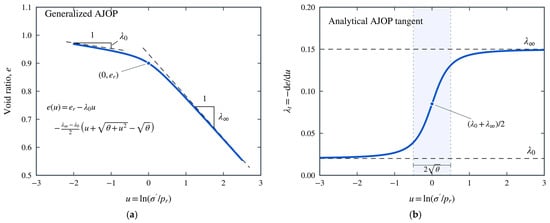
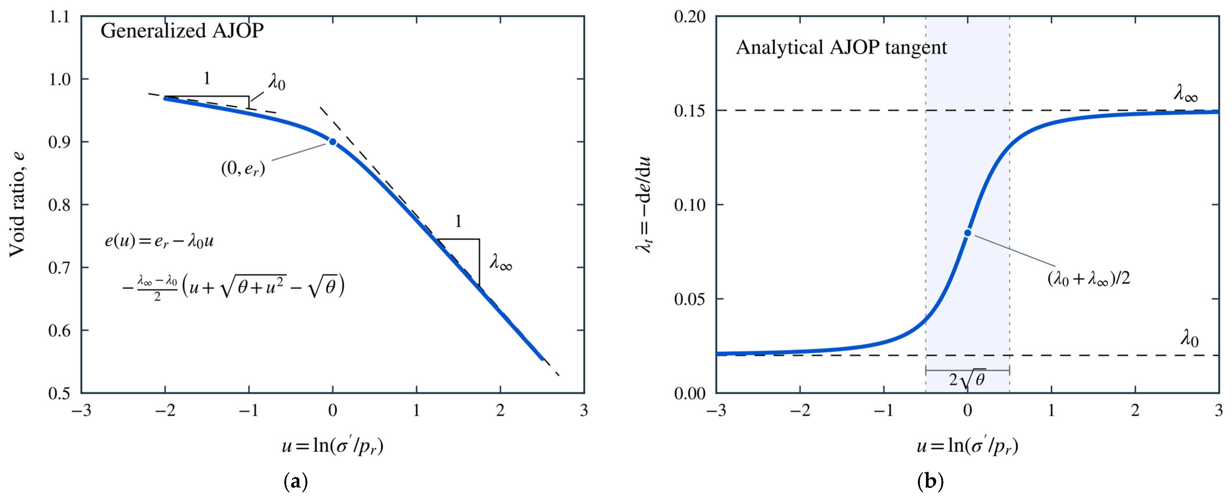
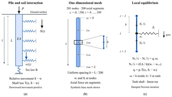
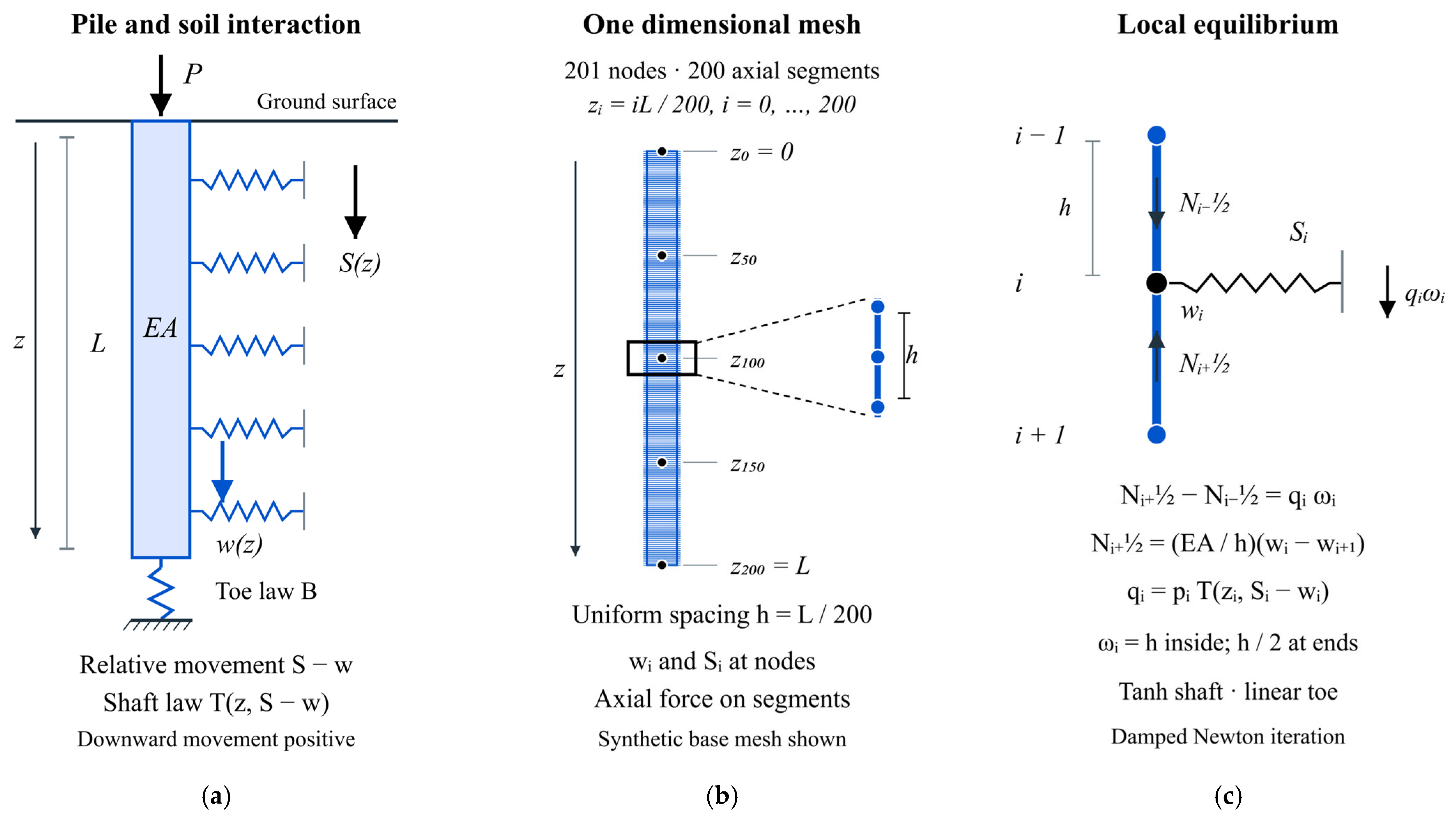
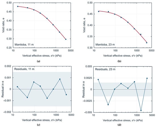
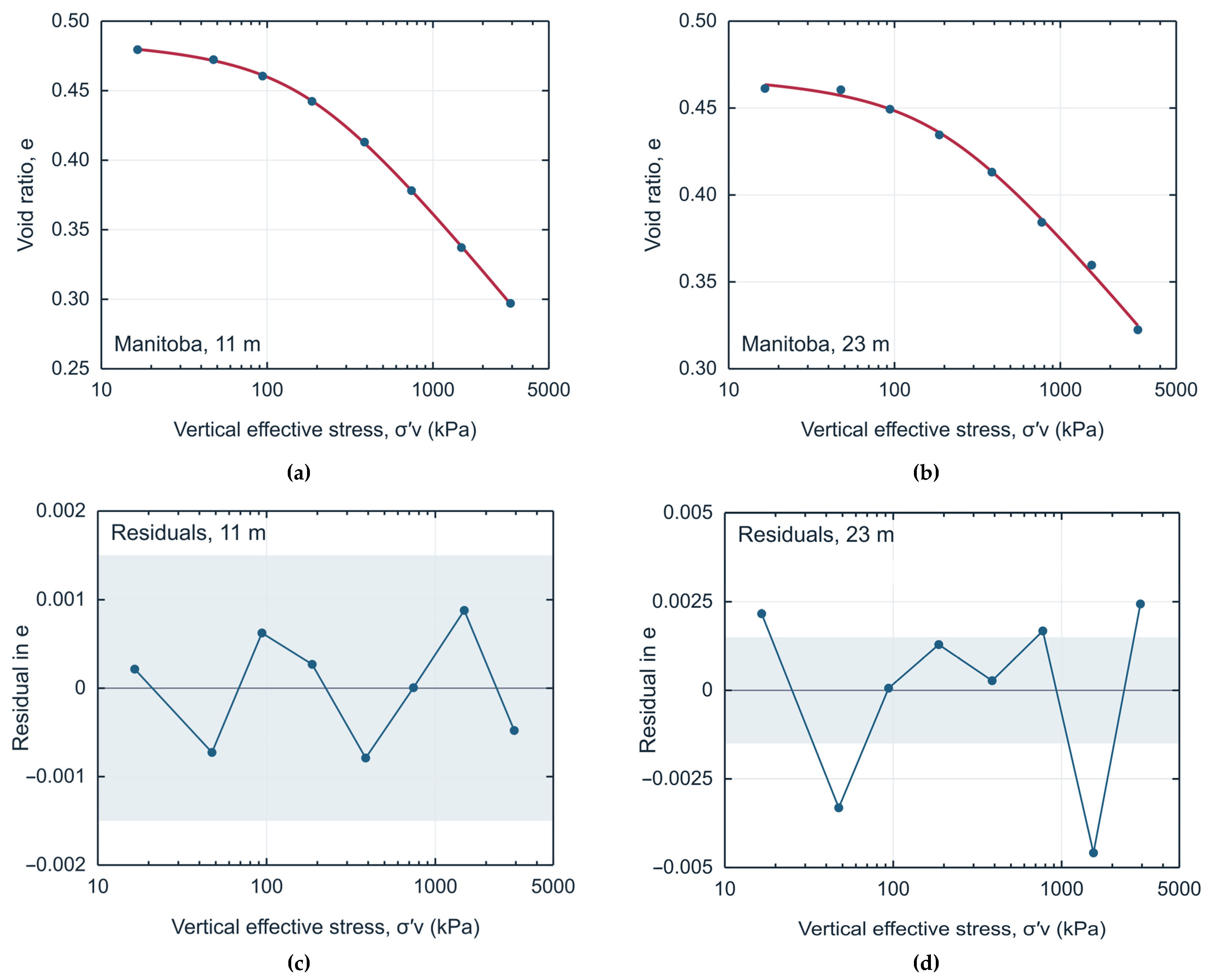
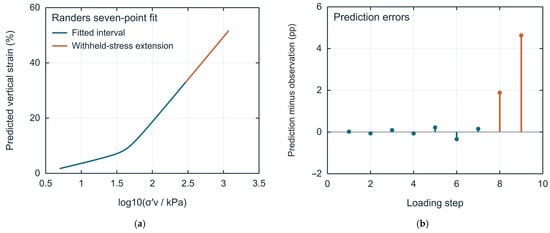
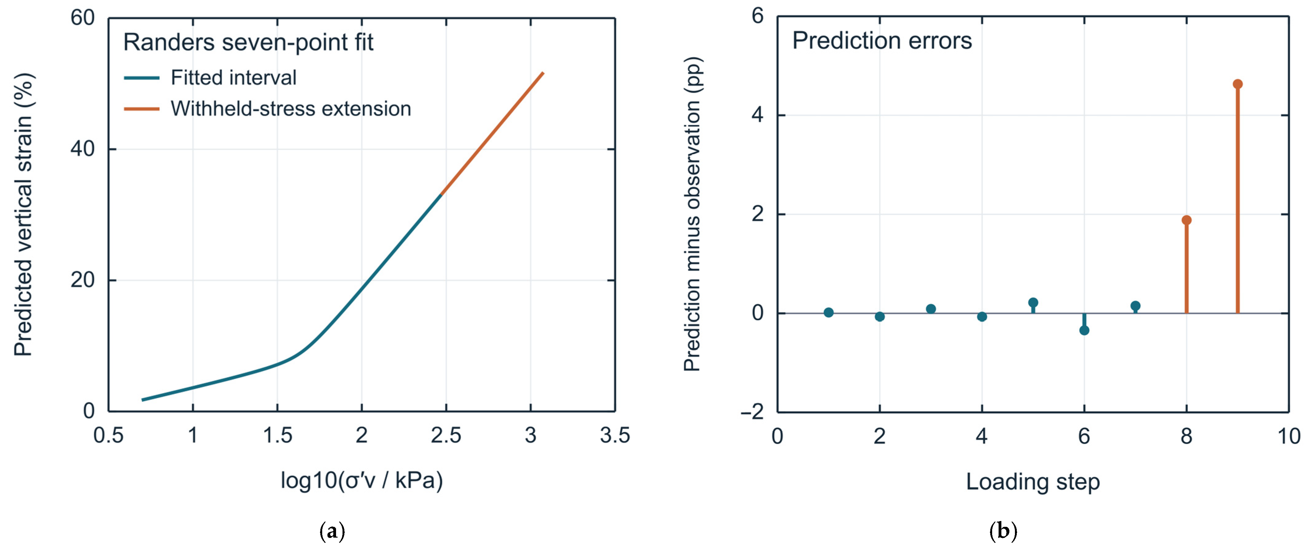
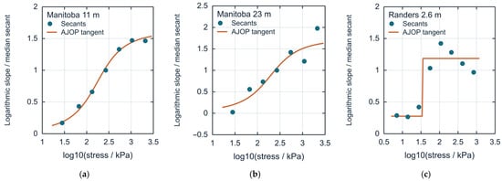
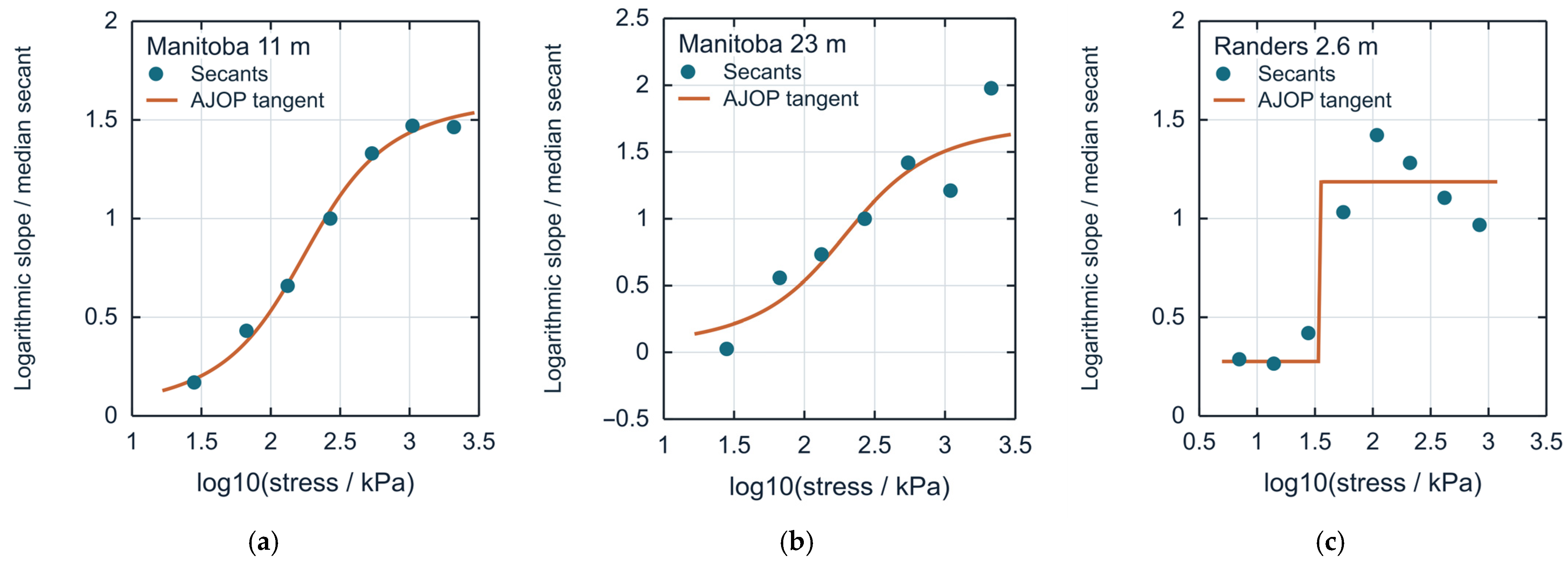
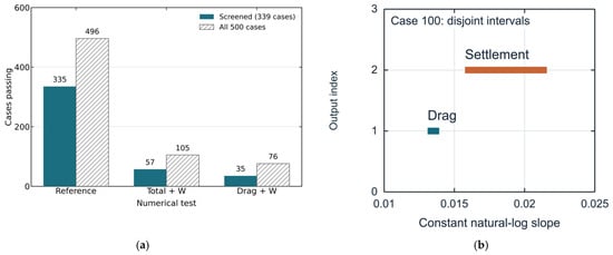
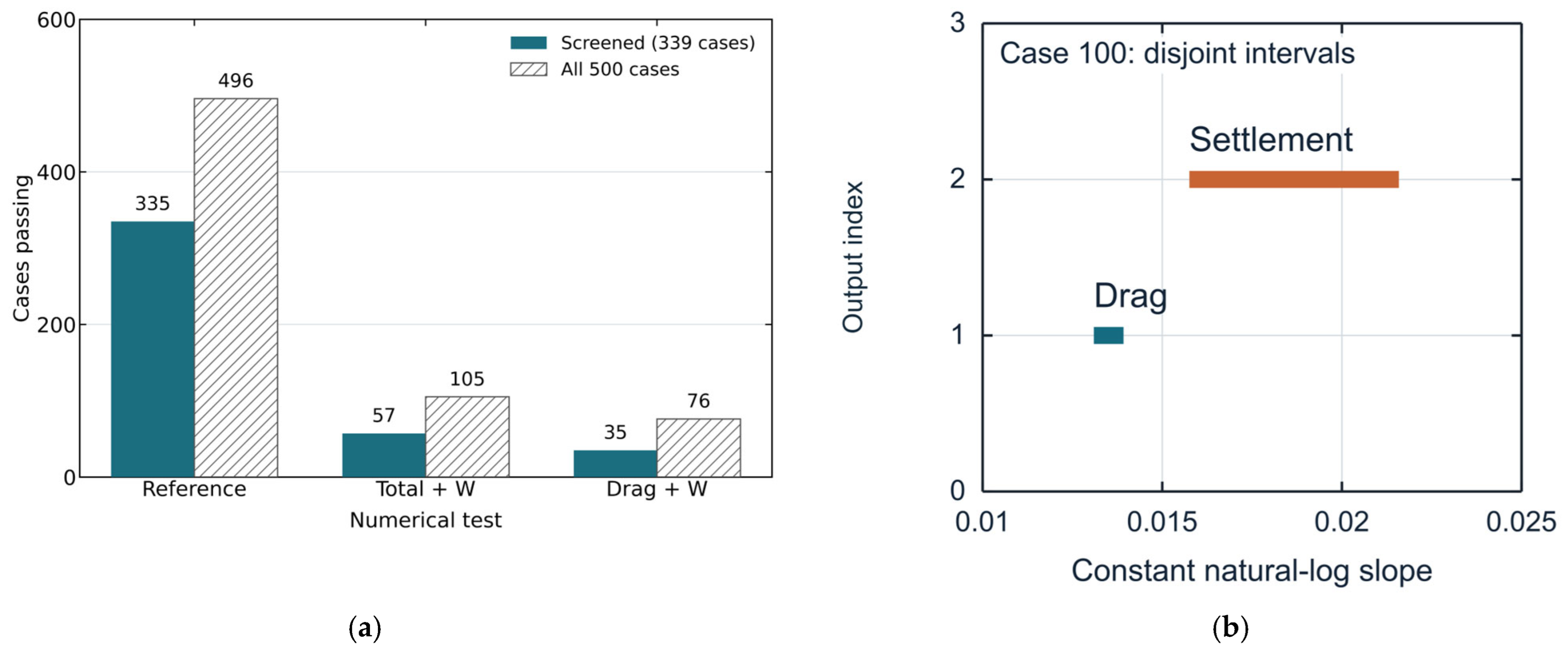
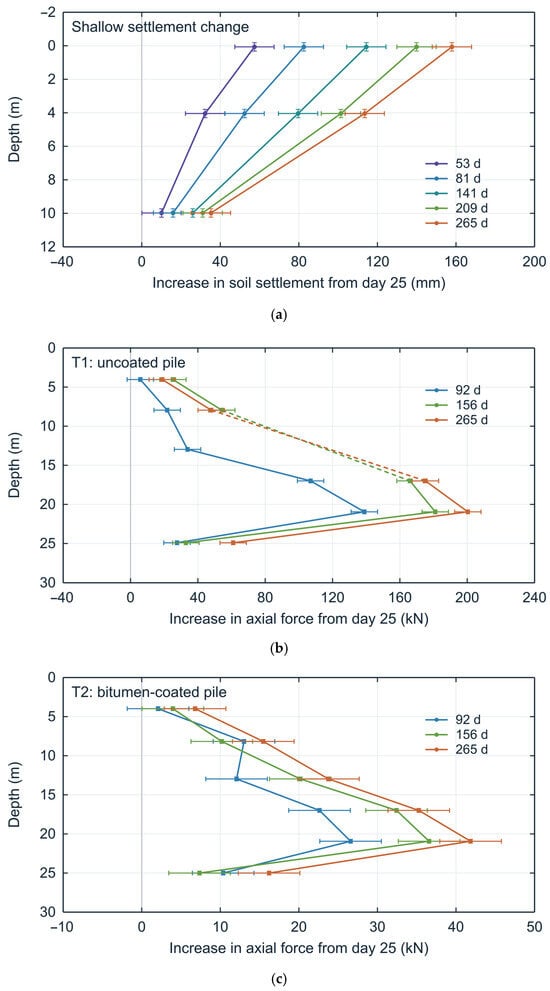
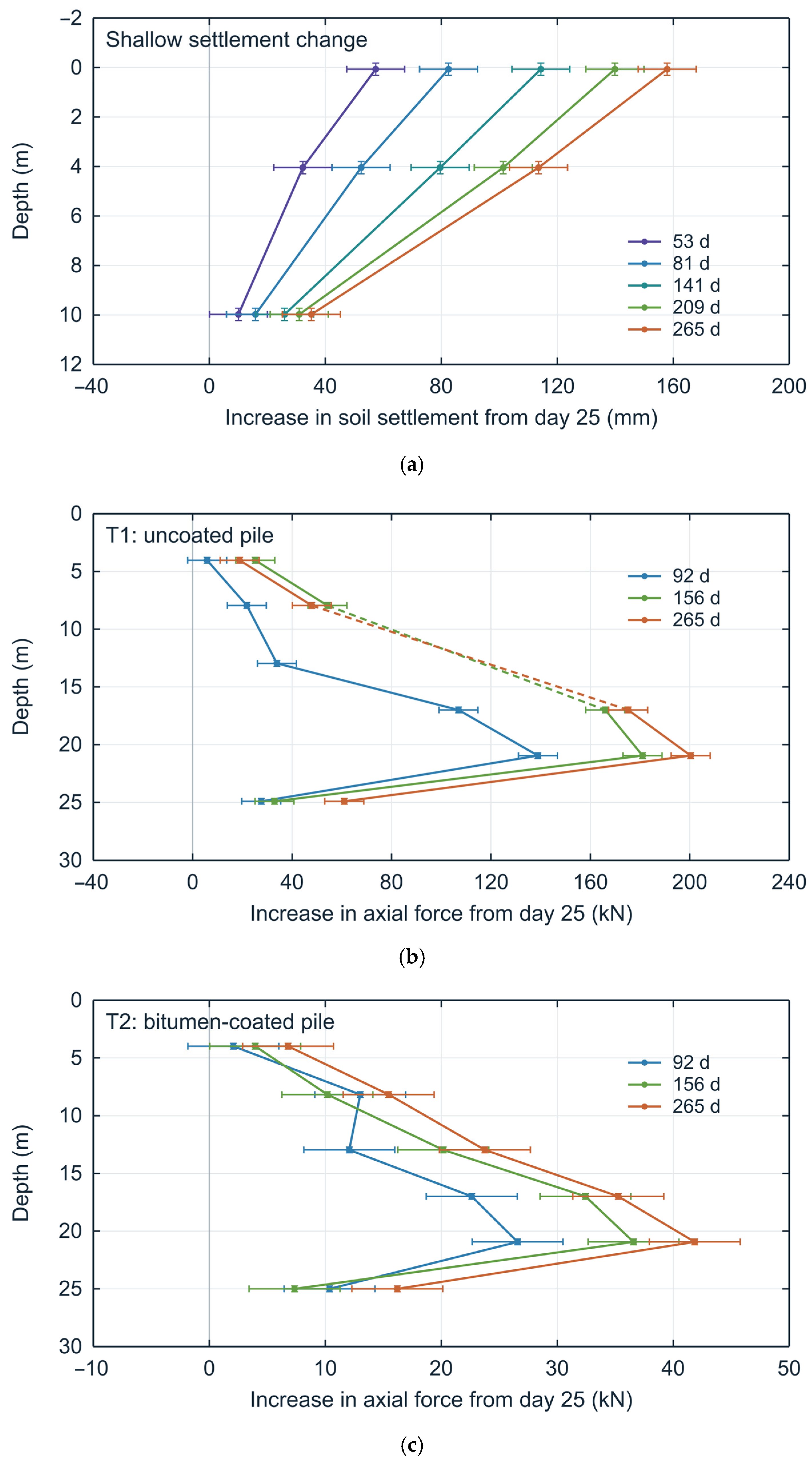
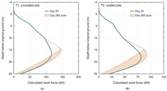
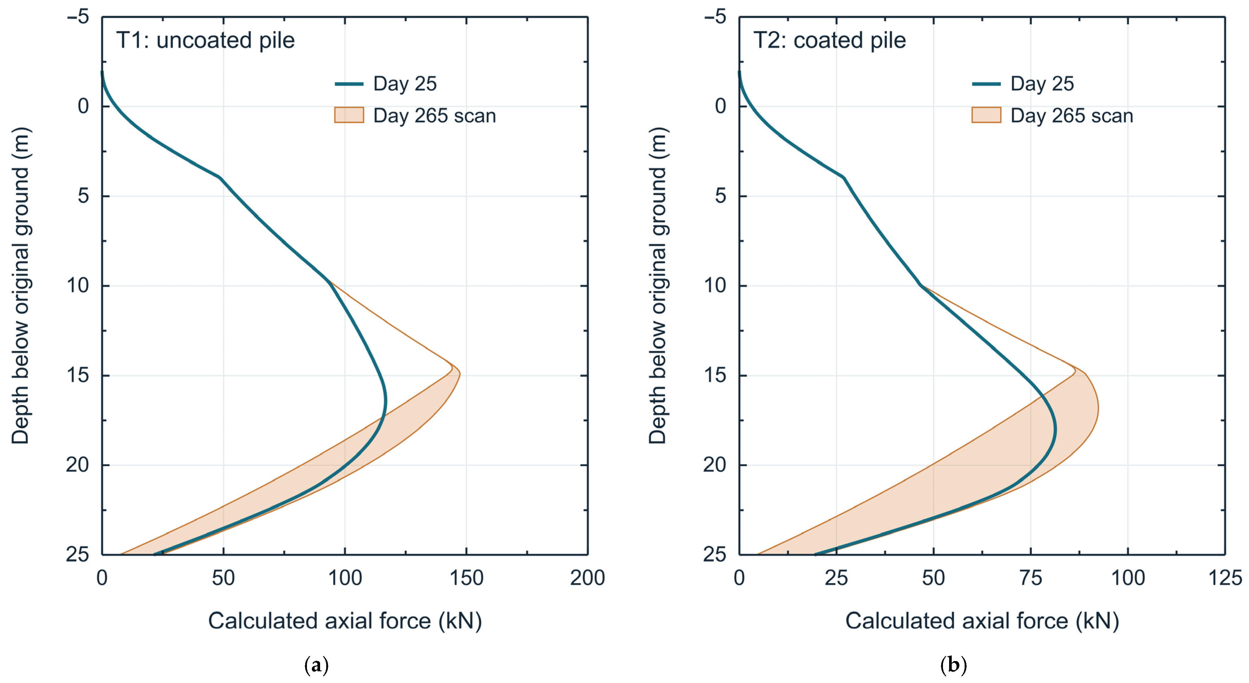
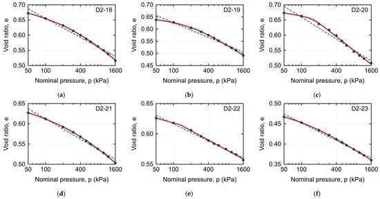
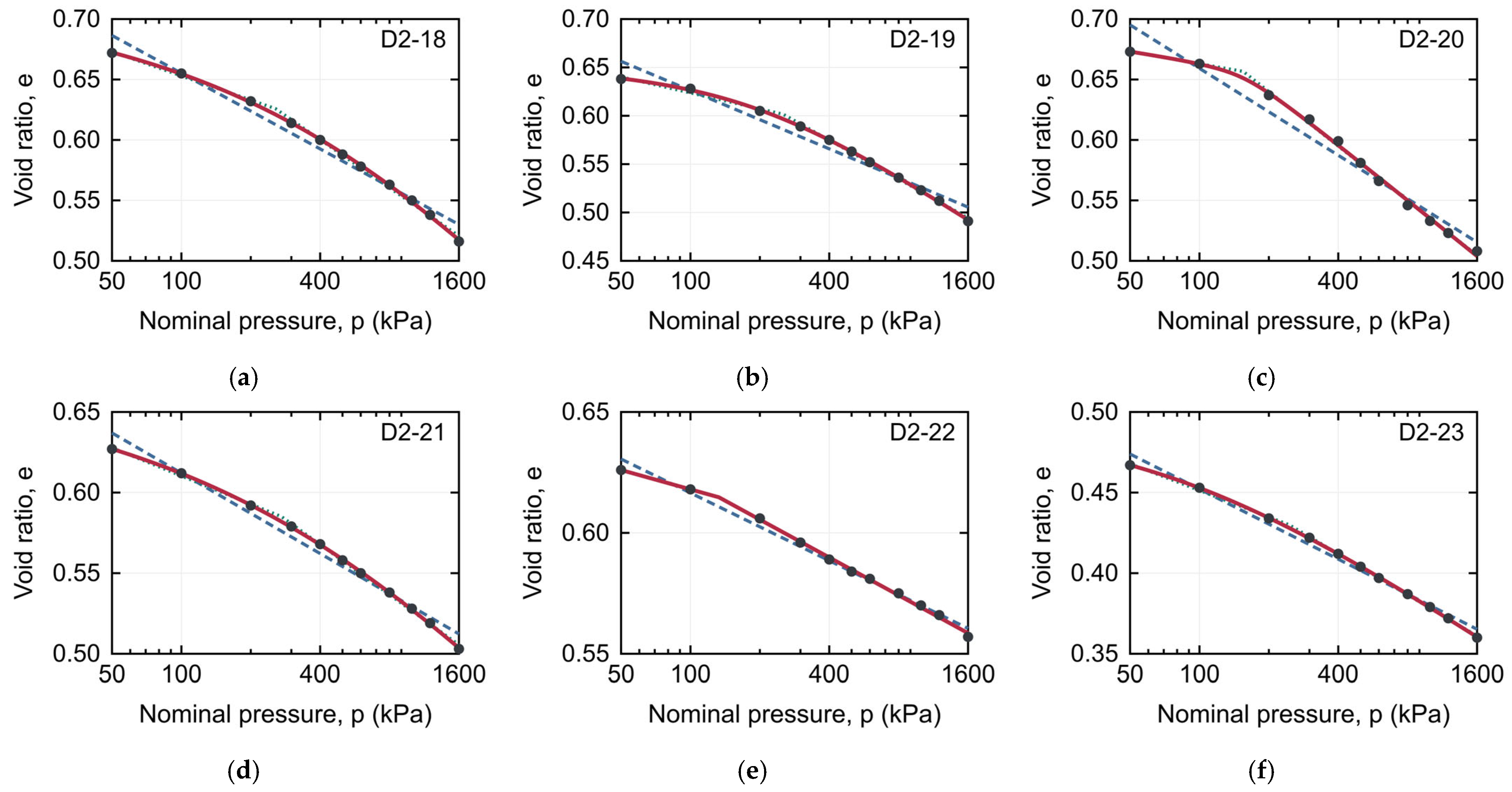

Disclaimer/Publisher’s Note: The statements, opinions and data contained in all publications are solely those of the individual author(s) and contributor(s) and not of MDPI and/or the editor(s). MDPI and/or the editor(s) disclaim responsibility for any injury to people or property resulting from any ideas, methods, instructions or products referred to in the content. |
© 2026 by the authors. Licensee MDPI, Basel, Switzerland. This article is an open access article distributed under the terms and conditions of the Creative Commons Attribution (CC BY) license.