Crack Detection and Adaptive Threshold Segmentation in Tunnel Linings Using Faster R-CNN and WOO-DELM

Abstract

Tunnel lining cracks are difficult to identify under uneven illumination, seepage marks, and complex surface textures. This study proposes a Faster R-CNN–WOO–DELM framework combining crack localization with adaptive threshold segmentation. Faster R-CNN localizes candidate crack regions, and five grayscale features are extracted from the candidate regions and valid background. A deep extreme learning machine (DELM) predicts an image-specific segmentation threshold, while the Wave Optics Optimizer (WOO) selects its regularization coefficient and stacking depth. The detection dataset comprised 2011 source images and their augmented versions. A threshold prediction subset comprising 1000 records with manually reviewed reference thresholds was constructed from the detection dataset. Faster R-CNN achieved an average precision of 0.874. On the held-out threshold test set, WOO-DELM achieved an RMSE of 0.021, a MAPE of 3.88%, an R² of 0.954, and an a10-index of 0.945, outperforming the comparison models in threshold prediction. For pixel-level segmentation, WOO-DELM achieves image-level mean IoU and Dice/F1 values of 0.8648 and 0.9266, respectively, across 30 independent test images, with corresponding standard deviations of 0.0519 and 0.0309. Under the specified sensitivity-analysis conditions, grayscale dispersion within candidate regions had the greatest influence on the predicted segmentation threshold. The proposed framework combines crack localization with image-specific threshold selection to delineate visible tunnel lining crack traces.

1. Introduction

Lining cracks are common defects in operational tunnels. Their spatial distribution, connectivity, and visible morphology provide important information for defect identification, delineation of repair sections, and structural condition assessment. Changes in surrounding rock pressure, traffic-induced vibration, concrete shrinkage, and temperature–humidity cycles may all contribute to crack initiation or propagation. At present, tunnel lining crack inspection still relies heavily on visual inspection and on-site measurements. The results are affected by illumination, imaging distance, and inspector experience, making low-contrast fine cracks and intersecting branches difficult to identify. Reliable crack identification therefore requires methods that can distinguish fine cracks from visually similar background features under variable imaging conditions.

Conventional image processing generally exploits grayscale differences between cracks and the concrete background to extract dark linear regions through filtering, edge detection, threshold segmentation, and morphological operations. These methods require relatively little computation and can produce clear contours under uniform illumination and simple background conditions. In practice, tunnel surfaces also contain construction joints, formwork textures, dust deposits, wet reflections, and shadows from facilities. Their local grayscale intensities and edge responses can resemble those of cracks. Previous studies have investigated the detection and identification of different types of tunnel surface defects [1,2,3] and have gradually extended deep learning methods to leakage and crack identification [4,5]. For crack detection under complex background conditions, subsequent studies have introduced data augmentation, feature learning, and image enhancement to improve recognition under different imaging conditions [6,7,8]. Other studies have examined the detection and quantitative analysis of structural damage and cracks in shield tunnels [9,10]. Overall, crack identification remains susceptible to surface conditions, background textures, and imaging conditions. When the global threshold is too low, fine cracks in bright regions may become discontinuous. When it is too high, dark stains and aggregate edges may enter the segmentation mask. Although local thresholding can alleviate illumination gradients, it may amplify rough textures within small windows. Determining a segmentation threshold from the foreground–background relationship of each image therefore remains a challenge for conventional tunnel inspection methods. Previous studies have advanced automatic inspection through lining defect detection, leakage segmentation, and two-stage defect identification [11,12,13]. With advances in computer vision, digital image-based crack identification, multiscale feature extraction, and improved object detection have gradually been applied to tunnel lining defect identification [14,15,16]. Studies have also explored the detection of voids behind linings, pixel-level crack monitoring, and visual inspection systems, providing different technical approaches to automatic defect inspection in underground engineering [17,18,19,20]. Nevertheless, crack localization and pixel-level segmentation remain insufficiently integrated under complex background conditions. Object detection can locate crack regions but cannot directly recover complete crack contours, whereas fixed-threshold segmentation is sensitive to variations in background grayscale intensity. A practical challenge is therefore to translate the candidate regions identified by object detection into crack masks while accounting for variations in foreground and background grayscale distributions.

Convolutional neural networks have shifted crack identification from manually designed features toward data-driven representations. Previous studies have applied improved U-Net and other deep learning methods to tunnel surface defect identification and crack analysis [21,22,23]. Researchers have subsequently developed deep learning- and Mask R-CNN-based detection and segmentation methods for defects on complex tunnel surfaces [24,25,26]. Further advances in pixel-level crack segmentation, convolutional neural network-based identification, and refined crack characterization have improved crack contour extraction under complex background conditions [27,28,29,30]. Object detection narrows the search area but cannot recover fine crack contours, whereas end-to-end segmentation generally requires detailed pixel-level annotations. This motivates combining detection-based spatial priors with grayscale statistics from candidate crack and background regions to predict image-specific segmentation thresholds.

Recent machine learning applications have also addressed structural performance prediction. Lazaridis and Thomoglou used interpretable models to estimate the shear capacity of textile-reinforced mortar-strengthened unreinforced masonry walls [31], while Gray et al. applied explainable machine learning to predict the ultimate shear capacity of cold-formed steel modular beams [32]. Although these studies focus on structural capacity prediction rather than image-based defect identification, they demonstrate the application of machine learning to engineering problems involving different types of input data and prediction targets.

This study develops an integrated Faster R-CNN–WOO–DELM framework for crack localization and adaptive threshold segmentation in tunnel linings. Faster R-CNN first identifies candidate crack regions, and five grayscale statistical features are extracted from the candidate regions and valid background. A DELM is trained to predict segmentation thresholds from these features, with WOO optimizing its regularization coefficient and stacking depth. The framework is evaluated through comparisons with alternative optimization and thresholding methods, followed by RBD-FAST sensitivity analysis to examine the influence of individual grayscale features on threshold prediction. The main methodological contribution lies in linking detector-defined foreground and background statistics to image-specific threshold prediction.

2. Data Sources and Sample Construction

2.1. Crack Images and Bounding-Box Annotation

The source images were obtained from the tunnel lining crack image dataset established by Feng et al. [30]. This dataset was compiled from on-site inspections of metro tunnels and publicly available tunnel images. The dataset covers various crack morphologies and lining surface conditions, making it suitable for evaluating crack identification and segmentation under heterogeneous background conditions. This study selected 2011 crack images as source samples, including longitudinal, circumferential, oblique, intersecting, and multibranch cracks, as well as challenging cases involving blurred edges, local discontinuities, and fine branches. Sample backgrounds include relatively smooth lining surfaces, rough textures, and local color variations to examine crack identification under different background conditions.

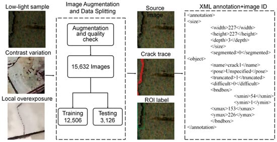
Considering the substantial variations in illumination, viewing angle, and surface conditions in operational tunnels, brightness adjustment, local contrast variation, sharpening, mild blurring, and simulated exposure changes were applied to expand the range of imaging disturbances and improve model adaptability to image quality and background conditions. Annotation validity was checked for each augmented image. Images with extensive saturation, visible interpolation artifacts, or unrecognizable main cracks were excluded. Training and testing use the selected tunnel-crack images and their augmented samples. The 2011 source images were first divided into training and independent test sets, and augmentation was then performed separately, yielding 15,632 images: 12,506 for detector training and 3126 for independent testing. The partition is defined by source-image identity, with each original image and all its augmented versions assigned to the same subset. Source-image identifiers, subset assignments, and augmentation types were retained and reused when constructing the subsequent threshold prediction dataset.

Bounding boxes were annotated using LabelImg (version 1.8.6), an open-source graphical image annotation tool used to draw rectangular boxes around objects and save their class labels and box coordinates as XML files [33]. The dominant crack orientation was first identified, and a tight rectangular box was drawn around each continuous main crack. Construction joints, stains, and shadows were not labeled as cracks, and spatially separated crack segments received separate boxes. After the first annotation round, the annotations were reviewed for completeness of crack ends, proportion of background within each box, and class consistency. An XML file with the same base name as each image was generated to record image dimensions, class labels, and bounding-box coordinates. These files were used both to train Faster R-CNN and to define the spatial regions for subsequent grayscale statistics inside and outside the boxes. Figure 1 presents the sample augmentation, data splitting, and bounding-box annotation workflow.

Figure 1. Workflow for tunnel lining crack sample augmentation, data splitting, and bounding-box annotation.

2.2. Threshold Prediction Dataset

A total of 1000 threshold prediction records were constructed by selecting 800 images from the detector training set and 200 from the independent detector test set. Sampling accounted for different crack morphologies and illumination disturbances, and no source image or its augmented versions appeared in both subsets. The manually annotated bounding boxes recorded in the XML files were used to define the candidate crack regions for grayscale feature extraction. Specifically, AGIF and SDIF were calculated within the annotated boxes, while AGIB and SDIB were calculated in valid lining regions outside these boxes. EDIR was calculated within the candidate regions. If an image contained multiple overlapping annotated boxes, the candidate regions were merged before feature calculation. The reference threshold for each image was determined by manually comparing binary segmentation results obtained with different candidate thresholds. The 800 training records were used for DELM fitting and hyperparameter search within the training set, whereas the 200 test records were reserved for final evaluation and did not participate in training. The subsequent distribution, correlation, and model comparisons all use the same dataset.

The 800 training records and 200 threshold test records use features extracted from manually annotated boxes. In the automated workflow, Faster R-CNN supplies the predicted boxes that define the candidate crack and surrounding background regions. The same five grayscale feature definitions are applied to these regions before threshold prediction. Localization performance is evaluated in Section 4, threshold prediction in Section 5.4, and the final crack segmentation in Section 5.5.

Three evaluators independently reviewed the candidate thresholds and corresponding binary segmentations, considering main-crack continuity, fine-branch retention, and suppression of noncrack background components. Thresholds were expressed on a 0–1 scale. If the largest and smallest thresholds selected by the three evaluators differed by more than 0.02, the original grayscale image and binary results were jointly re-examined, and the final reference threshold was collectively confirmed.

The five input features are defined from the detector-based foreground/background partition. Let V denote valid tunnel-lining pixels after excluding image borders, overlaid text, and other invalid areas. For candidate bounding boxes R_k(k = 1, …, K), let F = V ∩ (∪_k R_k) be the candidate foreground and B = V\F the surrounding valid background. Let g(p) be the grayscale intensity of pixel p on a 0–255 scale, with N_F = |F| and N_B = |B|. The average grayscale intensities of the candidate foreground (AGIF) and image background (AGIB) are

$$\mathrm{AGIF}={\displaystyle \frac{1}{N_F}}{\displaystyle \sum _{p\in F}g}(p),\hspace{1em}\mathrm{AGIB}={\displaystyle \frac{1}{N_B}}{\displaystyle \sum _{p\in B}g}(p)$$

(1)

The standard deviations of grayscale intensity in the candidate foreground (SDIF) and background (SDIB) describe the dispersion of pixel intensities in the respective regions. Using the population standard deviation, they are

$$\mathrm{SDIF}=\sqrt{{\displaystyle \frac{1}{N_F}}{\displaystyle \sum _{p\in F}{\left[g(p)-\mathrm{AGIF}\right]}^2}},\hspace{1em}\mathrm{SDIB}=\sqrt{{\displaystyle \frac{1}{N_B}}{\displaystyle \sum _{p\in B}{\left[g(p)-\mathrm{AGIB}\right]}^2}}$$

(2)

The extreme difference in grayscale intensity in the candidate region (EDIR) is the difference between the mean intensities of its brightest 1% and darkest 1% of pixels. Let g(i) be the i-th smallest grayscale intensity in F, and set k = ceil(0.01 N_F), where ceil denotes rounding up to the nearest integer. Then,

$$\mathrm{EDIR}={\displaystyle \frac{1}{k}}{\displaystyle {\displaystyle \sum _{i=N_F-k+1}^{N_F}}{g}_{(i)}}-{\displaystyle \frac{1}{k}}{\displaystyle {\displaystyle \sum _{i=1}^k}{g}_{(i)}}$$

(3)

If candidate boxes overlap, each shared pixel is counted only once in F. Averaging the two pixel groups allows EDIR to be non-integer even when the underlying pixel intensities are integers. These five features are computed from the grayscale image before the robust scaling described in Section 5.2. In the threshold-prediction dataset, F is determined from the annotated boxes; during automated inference, the detector-predicted boxes are used in the same definitions.

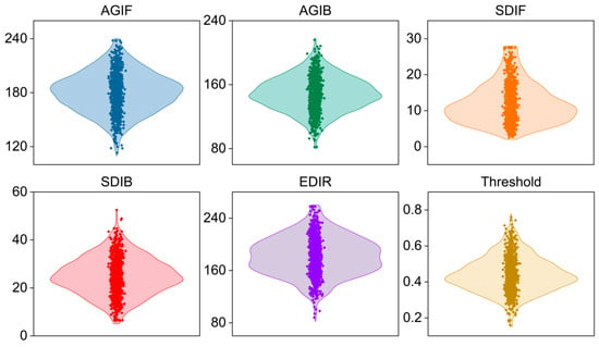
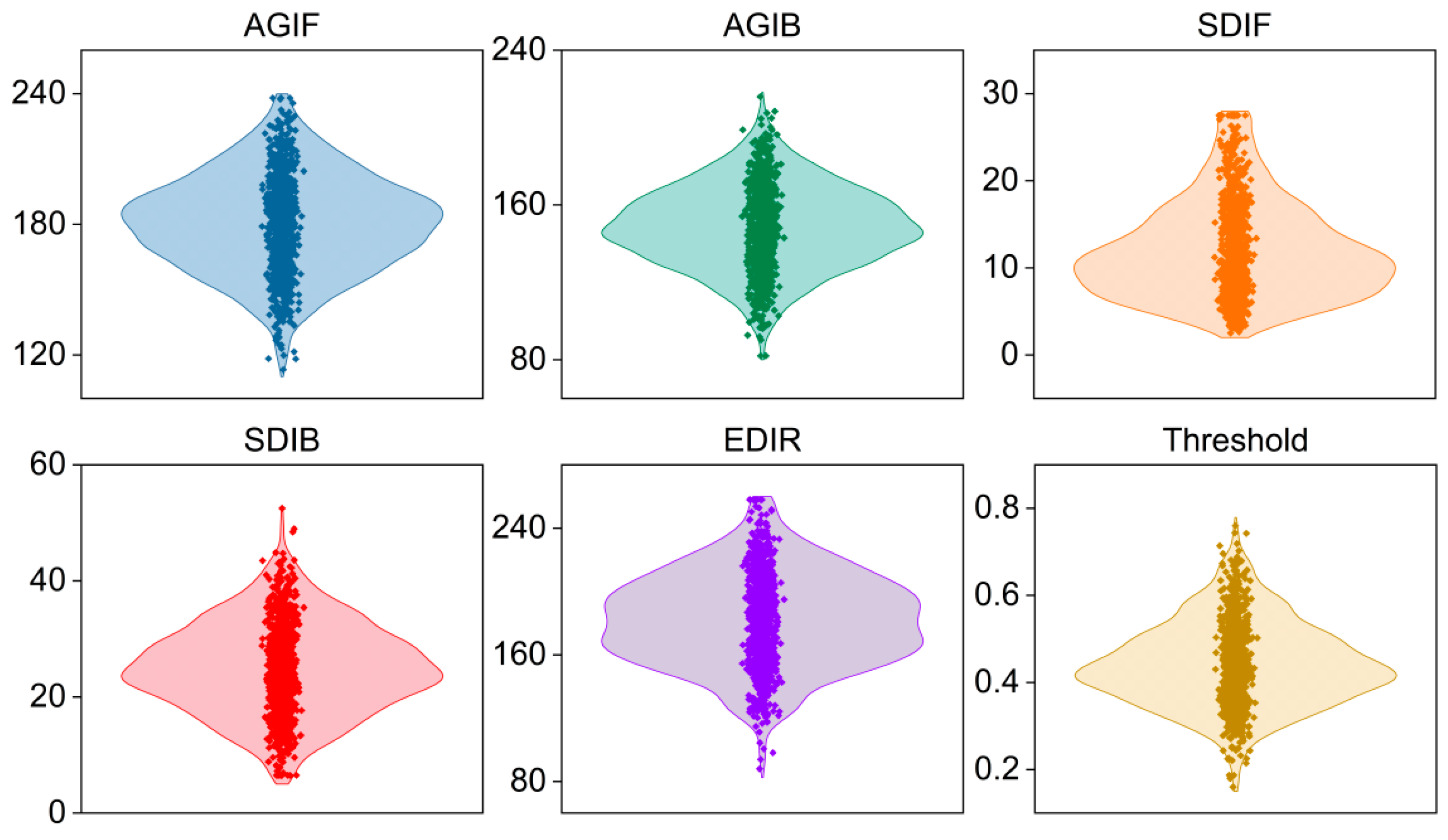
Figure 2 shows the marginal distributions of the five input variables and the manually reviewed threshold. AGIF and AGIB cover different brightness levels. SDIF and SDIB are right-skewed, indicating relatively strong local grayscale variations in a small number of images. EDIR spans a wide range, consistent with differences in exposure and surface texture. The manually reviewed thresholds are concentrated mainly in the middle of their range, with fewer samples near the upper and lower bounds. All variables fall within their predefined valid ranges, and no isolated outliers requiring removal were identified.

Figure 2. Distributions of six variables in the threshold prediction dataset.

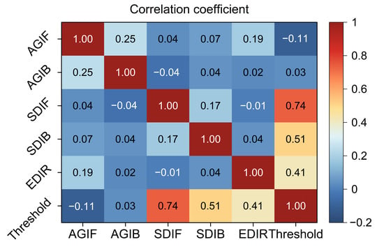
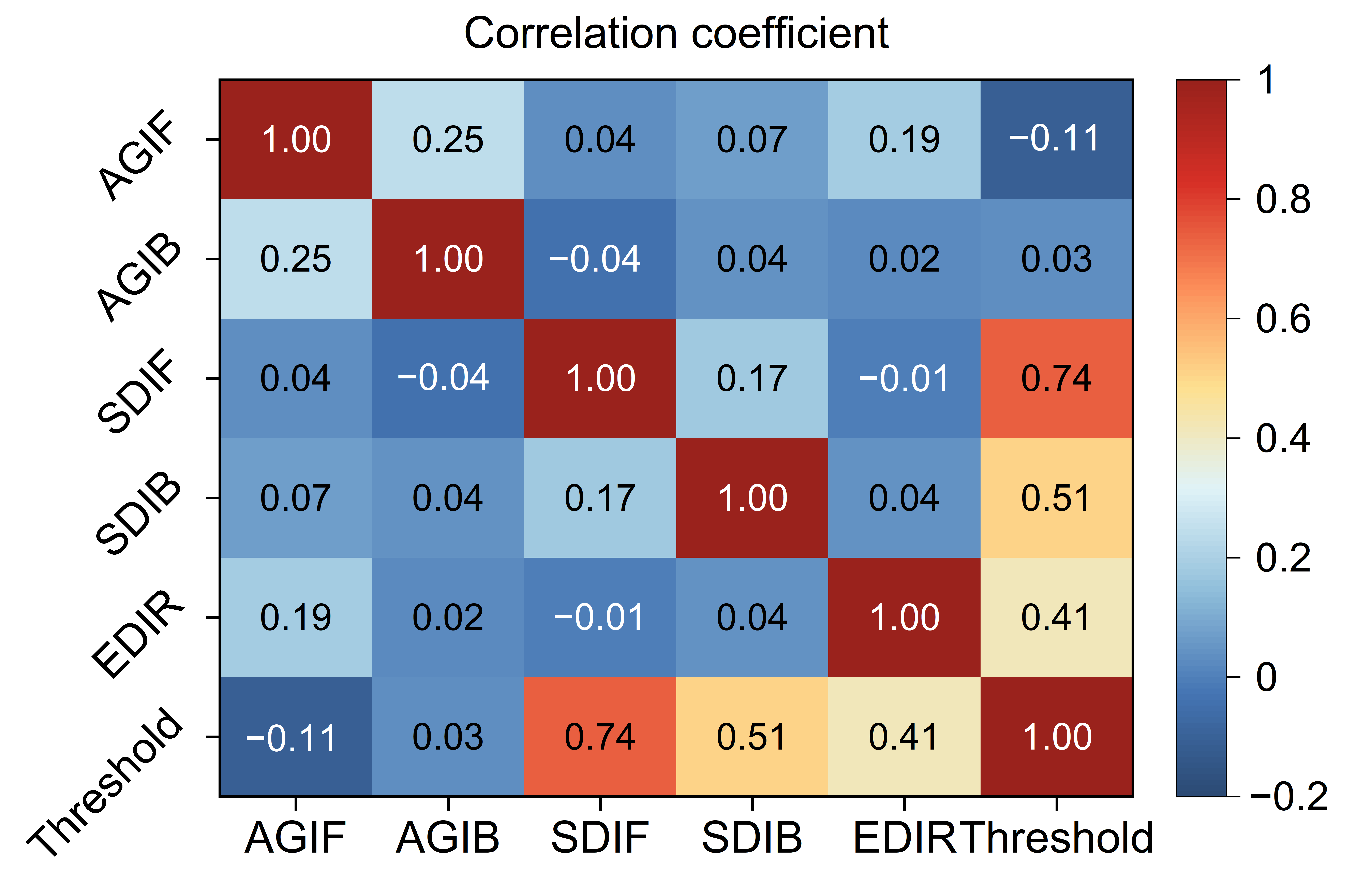
Figure 3 presents the Pearson correlation matrix. Overall, the five inputs show weak linear correlations. AGIF and AGIB are weakly positively correlated, reflecting the shared effect of illumination on foreground and background brightness. The manually reviewed threshold is most strongly correlated with SDIF (approximately 0.74), shows moderate correlations with SDIB and EDIR, and has weak linear relationships with the two mean-intensity variables. Correlation coefficients describe only pairwise linear relationships and do not capture interactions or local nonlinearities. DELM is therefore used to learn the nonlinear mapping between the five statistics and the manually reviewed threshold.

Figure 3. Pearson correlation matrix of the threshold prediction data.

3. Methodology

3.1. Crack Localization Using Faster R-CNN

Convolutional neural networks progressively extract edges, textures, and object-level semantic information through local receptive fields, weight sharing, and hierarchical features [34]. Faster R-CNN combines a region proposal network and a detection head on shared feature maps to generate proposals, classify objects, and regress bounding boxes [35]. A residual network is used as the backbone to alleviate gradient degradation as network depth increases [36]. The purpose of this stage is to narrow the search area for cracks, not to replace pixel-level contours with rectangular boxes.

After the input image is processed by the backbone to obtain multilevel feature maps, the region proposal network generates candidate boxes at different scales and aspect ratios and filters out obvious background regions using objectness scores. ROI feature pooling, classification, and coordinate regression are then applied, followed by non-maximum suppression to obtain the final crack boxes. Unlike classical edge detection and encoder–decoder segmentation methods [37,38,39], this stage does not directly recover crack contours. Instead, regions covered by detection boxes are defined as the candidate foreground, and the remaining valid lining regions are treated as background. Statistics from both regions are passed to the threshold prediction model. The candidate foreground defined here is the area covered by object detection boxes, not a pixel-level crack mask. Its grayscale statistics characterize the intensity distribution within the candidate regions.

Faster R-CNN uses an ImageNet-pretrained ResNet-50 backbone, feature layer activation_40_relu, one crack class, and a 512 × 512 × 3 input. Annotation boxes are transformed with image resizing. Nine anchors are estimated from the resized training boxes by IoU-distance clustering using seed 2024. Predicted boxes are mapped back to the original coordinates for feature extraction from the original 8-bit grayscale image.

The detector is trained end to end using SGDM, an initial learning rate of 0.001, momentum of 0.9, L2 regularization of 0.0001, a mini-batch size of 2, and 30 epochs. The learning rate is multiplied by 0.1 every 10 epochs, and batch-normalization statistics are frozen. Positive and negative training IoU ranges are 0.6–1 and 0–0.3, respectively; initialization and data-order randomization use seed 2024. Detection uses a confidence threshold of 0.45 and final non-maximum suppression with a Union IoU threshold of 0.50. Evaluation uses the box-matching IoU threshold of 0.50 defined in Section 4.

For detector training, the two-stage Faster R-CNN objective [35] combines region-proposal classification and box regression with RoI classification and box regression:

$$J_{\det }=J_{\mathrm{RPN},\mathrm{cls}}+J_{\mathrm{RPN},\mathrm{box}}+J_{\mathrm{RoI},\mathrm{cls}}+J_{\mathrm{RoI},\mathrm{box}}$$

(4)

The RPN classification term penalizes incorrect anchor objectness predictions using binary cross-entropy; the RoI classification term uses cross-entropy for crack versus background. The two box terms use the smooth L1 error between predicted and annotated box offsets, evaluated only for positive anchors or RoIs. Each term is averaged over its applicable sampled anchors or RoIs before summation. The XML annotations described in Section 2.1 provide the detector training targets.

3.2. Wave Optics Optimizer

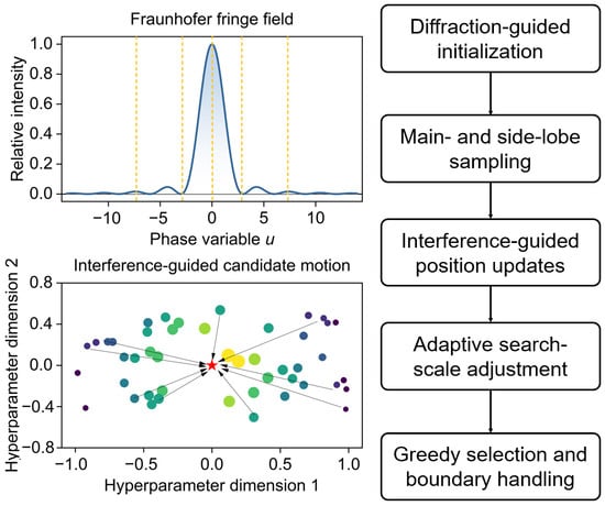
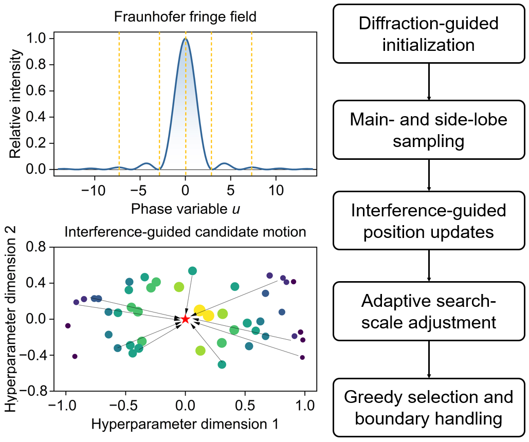
The Wave Optics Optimizer (WOO) uses principles of Fraunhofer single-slit diffraction and wave interference to organize the search for candidate solutions [40]. Here, the DELM regularization coefficient and number of stacked ELM-AE layers are encoded as a two-dimensional position, and the RMSE from five-fold cross-validation within the training set serves as the fitness value. Diffraction intensity controls the sampling density across intervals during initialization, while interference directions and a gradually decreasing search scale guide position updates. Figure 4 illustrates the WOO procedure used in this study.

Figure 4. Diffraction distribution, interference guidance, and candidate-solution update mechanism of WOO. (The red star indicates the current best solution, while the colored dots represent candidate solutions distributed across the hyperparameter search space.)

During initialization, candidate points are distributed nonuniformly, with a higher sampling density near the central diffraction lobe and additional points retained in the side-lobe intervals. This distribution maintains exploration across the search space without assuming that the optimal hyperparameters lie near its center.

The relative intensity and phase variable for single-slit diffraction are calculated using Equation (5), and the positions of dark fringes and approximate bright fringes are determined using Equation (6).

$$I(\theta )=I_0{\left({\displaystyle \frac{\sin u}{u}}\right)}^2,\hspace{1em}u={\displaystyle \frac{\pi d\sin \theta }{\lambda }}$$

(5)

$$\sin {\theta }_m^{(d)}={\displaystyle \frac{m\lambda }{d}},\hspace{1em}\sin {\theta }_m^{(b)}={\displaystyle \frac{(2m+1)\lambda }{2d}}$$

(6)

where I(θ) is the diffraction intensity in direction θ; I₀ represents the central maximum intensity; u denotes a dimensionless phase variable; d and λ are the slit width and wavelength, respectively; m is the fringe order; and θ_m(d) and θ_m(b) denote the positions of the mth dark and approximate bright fringes, respectively. In this study, λ = 5 × 10⁻⁴ mm, d = 1 × 10⁻² mm, and I₀ = 1. The limiting value is used when sinθ = 0. The bright- and dark-fringe intervals are linearly mapped to the actual hyperparameter ranges.

After iteration begins, the search scale changes with the number of remaining iterations. Early iterations allow candidate points to move across wider intervals to examine underexplored regions, whereas later iterations increase the search effort in currently promising regions. If candidate solutions become overly concentrated, a random component expands the search range to prevent all positions from remaining in the same local region.

The time control variable, phase, and intensity are updated at iteration t using Equation (7), and candidate positions are updated using Equation (8).

$$C_t=1-{\displaystyle \frac{t}{T}},\hspace{1em}{u}_i^t={\displaystyle \frac{\pi \Delta S_i^t}{\lambda }},\hspace{1em}{l}_i^t=l_0{\left({\displaystyle \frac{\sin u_i^t}{u_i^t}}\right)}^2$$

(7)

$${\tilde{X}}_i^{t+1}=B\left[X_i^t+{\mathrm{\Omega }}_i^t\odot Z_i^t\odot D_i^t\right]{ X}_i^{t+1}=argmi{n}_{X\in \{X_i^t,{\tilde{X}}_i^{t+1}\}}f(X)$$

(8)

where C_t is the time control variable; t and T are the current and maximum iteration numbers, respectively; ΔS_it and Iit are the displacement and relative intensity of the ith candidate light wave; X_it is the current candidate solution; ${\tilde{X}}_{i,t+1}$ is the new candidate solution; Ω_it is the step size in each dimension; Z_it is a random or local search direction; D_it combines distance and phase information between candidate solutions; ⊙ denotes elementwise multiplication; and B is the boundary mapping operator. A new position is accepted only if it reduces the five-fold cross-validation RMSE. After termination, the global best position determines the DELM parameters.

3.3. Deep Extreme Learning Machine

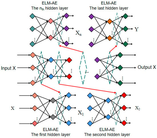
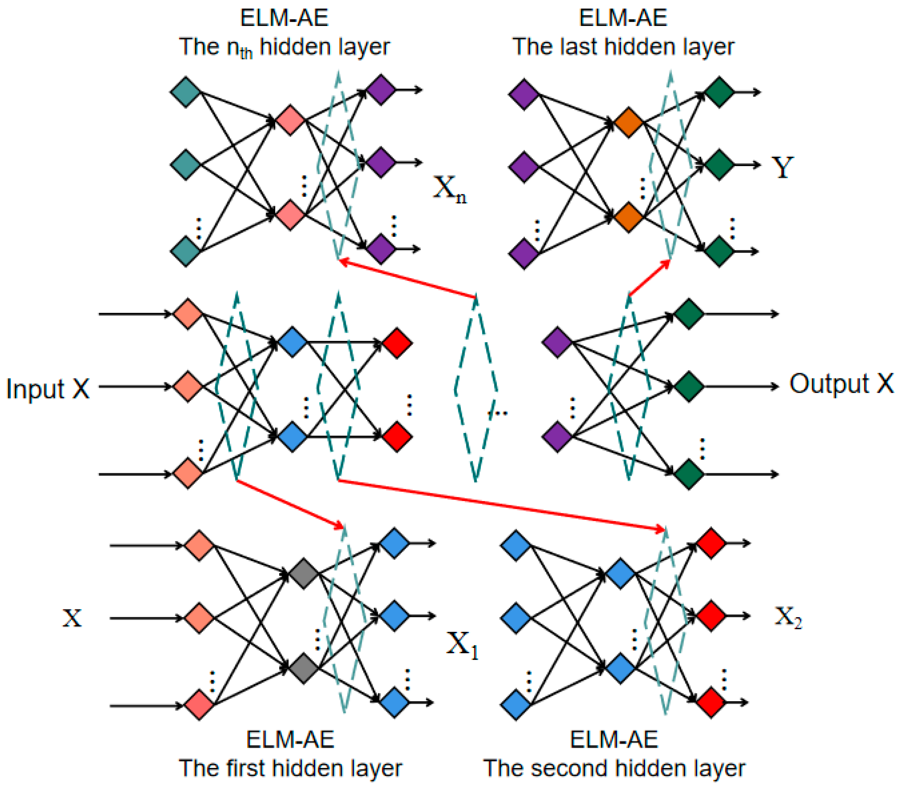
A deep extreme learning machine (DELM) consists of multiple stacked extreme learning machine autoencoders (ELM-AEs) and performs threshold regression on the resulting high-level representation. Conventional ELM randomly generates input weights and hidden-layer biases and obtains output weights analytically [41]. ELM-AE uses its input as the reconstruction target and can compress redundant information through unsupervised learning [42,43,44]. In this study, ELM-AEs are trained layer by layer, and the final feature representation is passed to a regression output layer to predict the segmentation threshold. WOO and the other optimization algorithms adjust only the regularization coefficient and stacking depth; the definitions of the five grayscale statistics and the data split remain unchanged. Figure 5 shows the network architecture.

Figure 5. Schematic of stacked ELM-AE representation learning in DELM.

The DELM training objective has two parts. At ELM-AE layer j (j = 1, …, L), the layer input X_j is reconstructed from the randomly generated hidden-layer output H_j by fitting output weights B_j. With the regularization coefficient C, the reconstruction cost is

$$J_{\mathrm{AE}}^{(j)}(B_j)={\displaystyle \frac{1}{2}}{‖H_j{B}_j-X_j‖}_F^2+{\displaystyle \frac{1}{2C}}{‖B_j‖}_F^2$$

(9)

After the L ELM-AE layers have been fitted sequentially, let Z_L denote the final representation of the training records, y the vector of manually reviewed thresholds, and w the linear threshold-regression weights. The supervised regression cost is

$$J_{\mathrm{reg}}(w)={\displaystyle \frac{1}{2}}{‖Z_{L}w-y‖}_2^2+{\displaystyle \frac{1}{2C}}{‖w‖}_2^2$$

(10)

The first terms in these expressions penalize reconstruction and threshold-prediction errors, respectively; the second terms are L2 penalties on the fitted weights. The same candidate C is used in the ELM-AE layers and the final regression layer. The layer-wise output weights and final regression weights are obtained by regularized least squares for each candidate (C, L); WOO selects C and L rather than directly updating these weights.

3.4. Integrated Faster R-CNN-WOO-DELM Framework

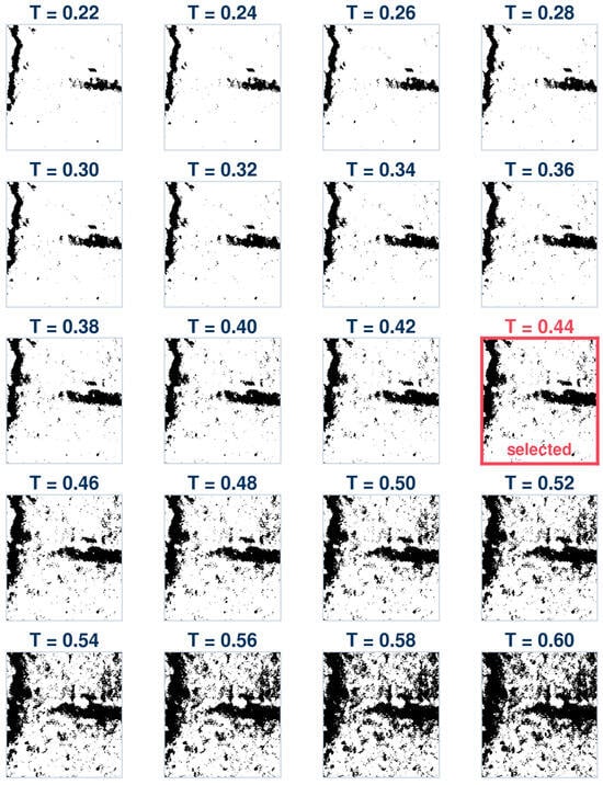
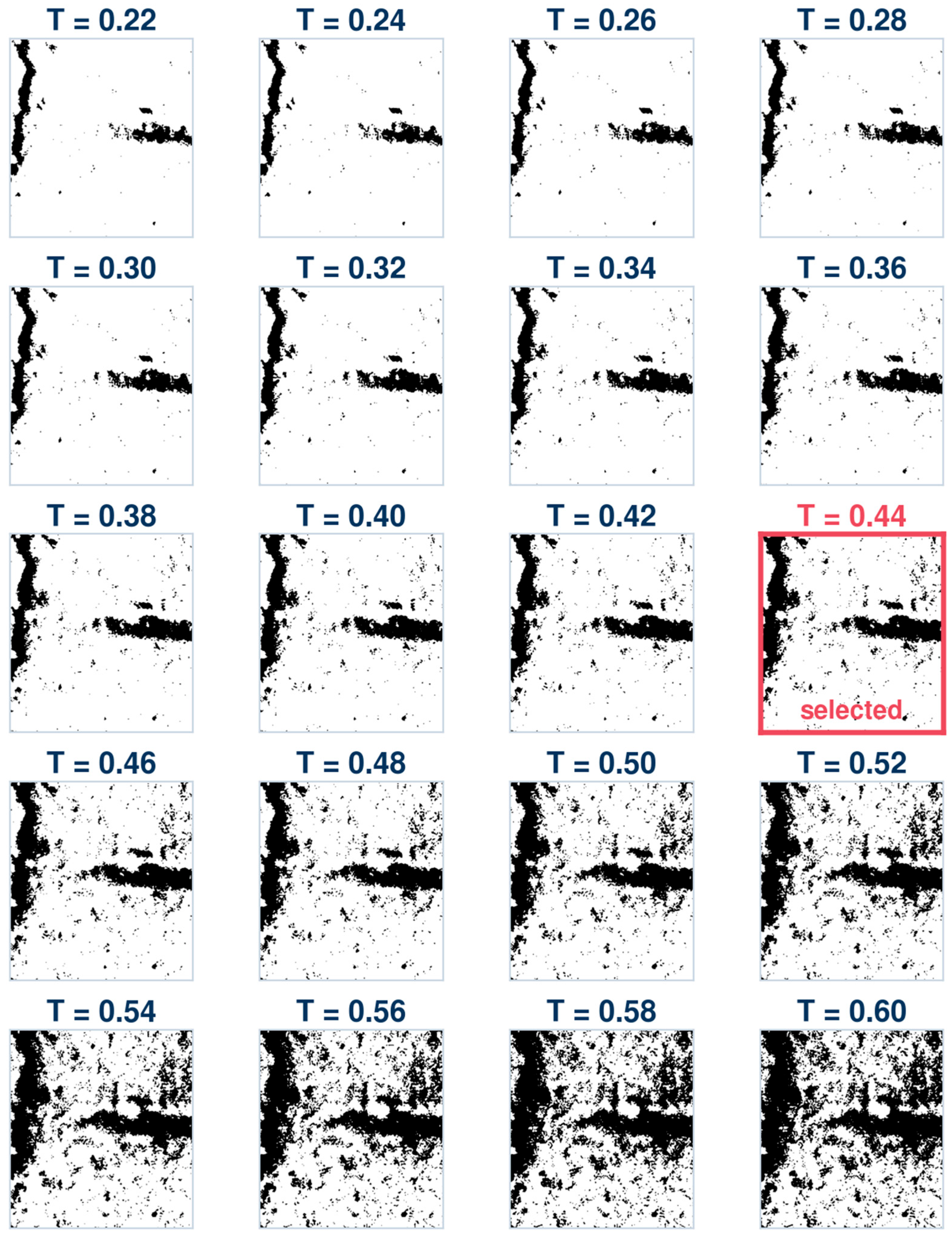
The predicted threshold converts a grayscale image into a binary crack mask. The statistics are recorded on the original 8-bit grayscale scale of 0–255, whereas the predicted threshold T is expressed on a scale of 0–1. Before segmentation, pixel intensity g is normalized to g/255, and pixels satisfying g/255 ≤ T are labeled as dark crack pixels. Similarly, an 8-bit threshold t obtained using Otsu’s method is converted to t/255 before segmentation. If the threshold is too low, low-contrast cracks and fine branches may become disconnected or be missed. If it is too high, noncrack regions such as wet patches, aggregate edges, and shadows may be incorrectly retained, producing false detections and distorted contours. Figure 6 shows how the contours of the same image change over a threshold sequence of 0.22–0.60. At T = 0.44, the main crack and fine branches remain connected, while most background particles are suppressed. Considering retention of the main crack and fine branches together with background-noise suppression, T = 0.44 is selected as the manually determined reference threshold for this sample. The review also considers main-crack connectivity, retention of fine branches, and the number of noncrack connected components.

Figure 6. Binary contours of tunnel lining cracks at different thresholds. The red box indicates the selected reference threshold (T = 0.44).

The thresholding step produces an initial binary mask before connected-component filtering and morphological cleanup. For a pixel at coordinates (x, y), the assignment can be written as

$$M_0(x,y)=\left\{\begin{array}{cc}1,\hfill & g(x,y)/255\le T,\hfill \\ 0,\hfill & g(x,y)/255>T.\hfill \end{array}\right.$$

(11)

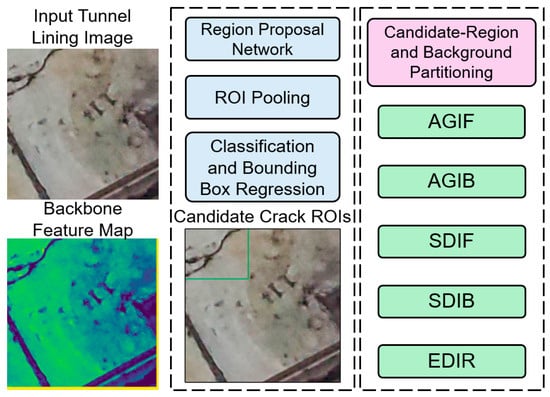
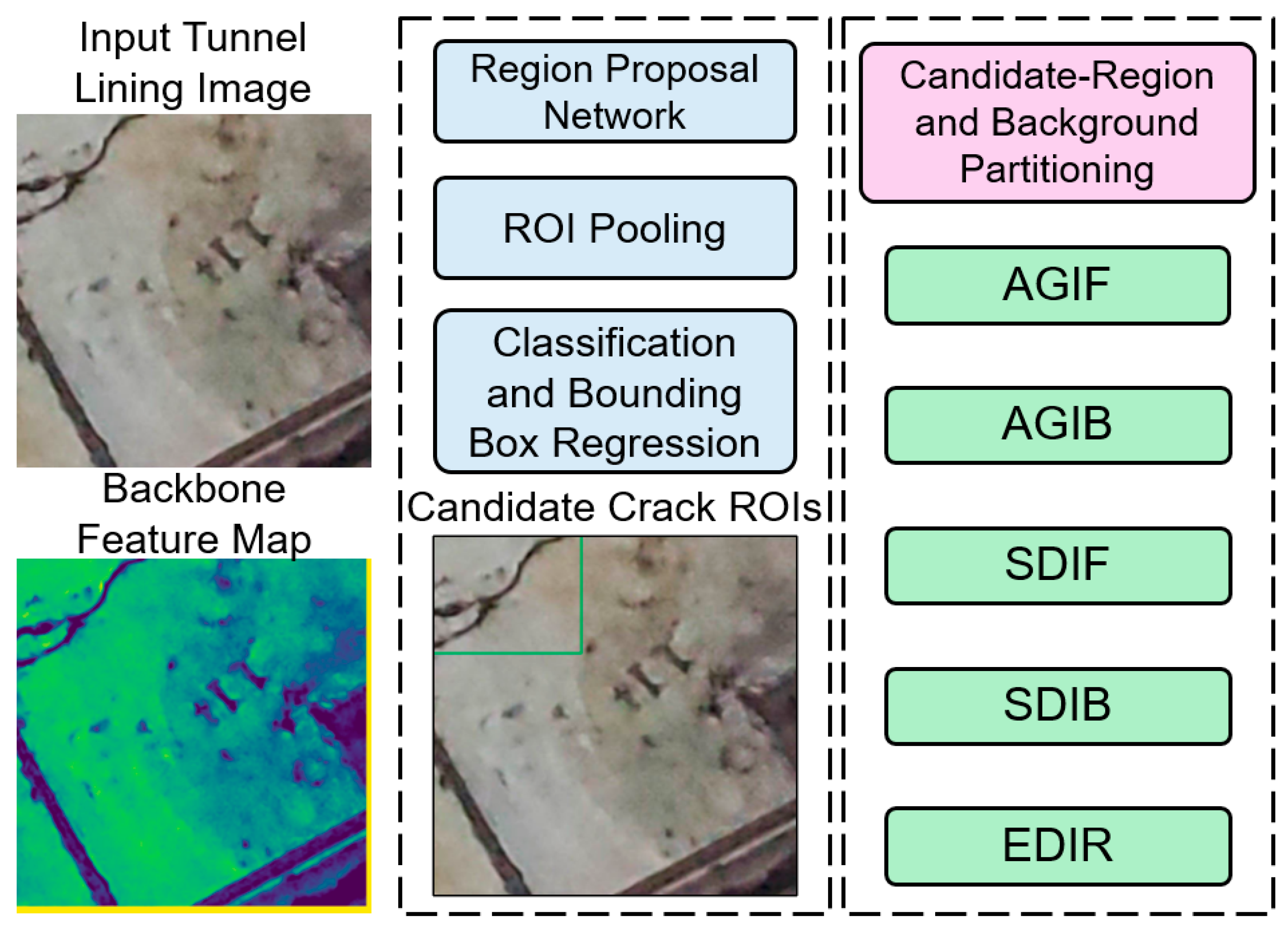
Faster R-CNN identifies candidate crack regions for grayscale feature extraction, and WOO-DELM predicts an image-specific threshold from these features. The predicted threshold is then applied to the entire grayscale image rather than being restricted to the detected bounding boxes. In the initial mask above, a value of 1 denotes a dark pixel selected by that threshold, not independent proof that the pixel is a crack. After connected-component filtering and morphological cleanup, the binary result allows the visible trace, approximate contour, main-crack continuity, and retention of fine branches to be inspected at the pixel level. These properties support the visual comparison in Section 5.5.

Figure 7 presents the integrated workflow. After Faster R-CNN outputs the crack boxes, AGIF and SDIF are calculated inside the boxes, AGIB and SDIB in valid lining regions outside the boxes, and EDIR in the candidate regions. The five statistics form the DELM inputs, and the manually reviewed threshold serves as the supervised output. During training, WOO searches for the regularization coefficient and the number of stacked ELM-AE layers. During prediction, statistics from the current image are passed to the trained model. Once a threshold is obtained, binarization, connected-component filtering, and morphological cleanup are performed in sequence. If an image contains multiple overlapping boxes, the foreground regions are merged before calculating statistics. The background includes only pixels outside the boxes and excludes invalid content such as border text. Notably, regions covered by detection boxes are treated as the candidate foreground, rather than as ground-truth crack masks. Because each box inevitably contains some background pixels, the extracted grayscale statistics reflect the combined intensity distribution of the candidate crack region and its surrounding background. DELM does not directly identify individual crack pixels. Instead, it learns the nonlinear relationship between these regional statistics and manually reviewed thresholds to determine an adaptive threshold for subsequent binarization.

Figure 7. Faster R-CNN crack localization and grayscale statistical feature extraction workflow.

3.5. Implementation and Computing Environment

The computational workflow was implemented in MATLAB R2024b [45], including image processing, grayscale-feature extraction, model fitting, hyperparameter search, and evaluation of detection and threshold-prediction results. The sequence of operations is described in Section 3.4, with the DELM training and WOO parameter-selection objectives detailed in Section 3.3 and Section 5.2.

The official MathWorks documentation for Faster R-CNN network construction and training is cited as the software reference for the detection stage [46]. These software citations identify the computational environment and implementation resources, complementing the algorithmic references in Section 3.1, Section 3.2 and Section 3.3. LabelImg, used for bounding-box annotation and XML generation, is referenced separately in Section 2.1 [33].

Experiments were conducted in MATLAB R2024b on 64-bit Windows 11 with an Intel Core i7-12700 CPU, 32 GB RAM, and an NVIDIA RTX 3060 GPU (NVIDIA Corporation, Santa Clara, CA, USA) with 12 GB memory. Detector training and inference use the GPU; DELM fitting and all hyperparameter searches use the CPU without a parallel pool. The data partition follows Section 2.1. Binary post-processing uses 8-connectivity, removes components smaller than eight pixels, and applies one closing operation with a 3 × 3 square element at the original image resolution.

Offline computation comprises detector training, cross-validated hyperparameter search, and final DELM refitting. Per-image inference uses the fitted models and training-derived scaler without rerunning WOO. Inference timing starts with an image in memory and covers preprocessing, detection, feature extraction, threshold prediction, and binary post-processing; disk access and display are excluded. After 10 warm-up passes, the same 100 test images are processed five times, with GPU synchronization before and after timing. For each of the 100 test images, five inference times were averaged. The mean and sample standard deviation across these image-level means were 0.183 ± 0.027 s per image for the complete in-memory workflow. Offline search is timed separately (Section 5.3) and excluded.

4. Detection Results and Accuracy Evaluation

A successful detection is determined by matching a predicted crack bounding box to a manually annotated ground-truth box on the independent detector test set. Their box-level intersection over union (IoU) is

$$\mathrm{IoU}(B_p,B_{gt})={\displaystyle \frac{A(B_p\cap B_{gt})}{A(B_p\cup B_{gt})}}$$

(12)

Here, B_p is the predicted box, B_gt is an annotated box, and A denotes the area of a region. After non-maximum suppression, predictions are ranked by confidence. For each prediction in descending order, the annotated box with the highest IoU is identified. The prediction is a true positive (TP) if this IoU is at least 0.50 and that annotated box has not already been matched. Otherwise, including when the best-matching crack has already been assigned to a higher-confidence prediction, it is a false positive (FP). Each annotated box left unmatched is a false negative (FN). This criterion evaluates box localization rather than pixel-level crack segmentation.

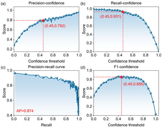
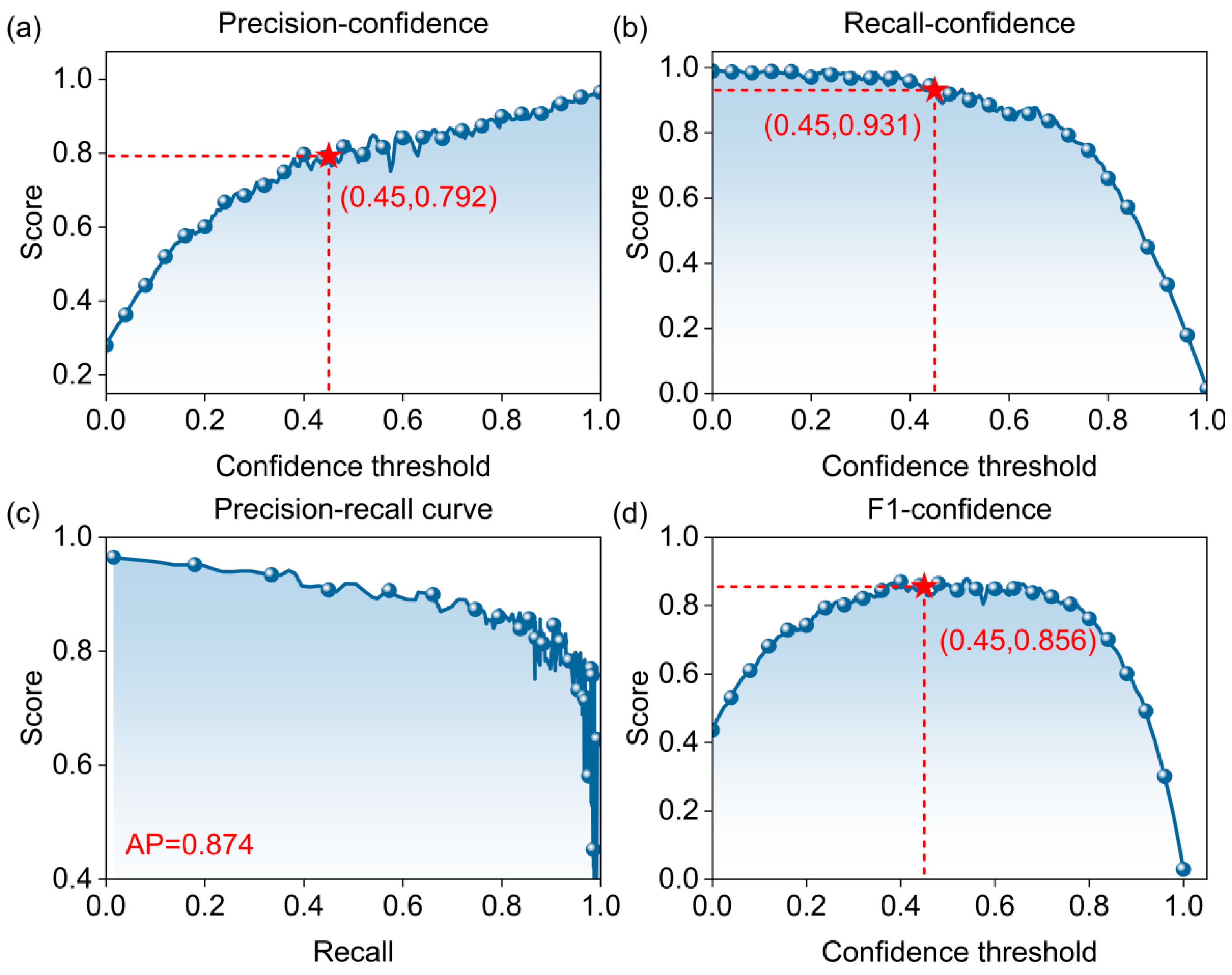
For the operating point in Figure 8, predictions with confidence scores of at least 0.45 are retained for precision, recall, and F1 calculation. The precision–recall curve and AP are obtained by varying the confidence cutoff while keeping the box-matching IoU threshold fixed at 0.50. Thus the confidence cutoff filters predictions, whereas the IoU threshold decides whether a retained prediction matches a crack.

Figure 8. Faster R-CNN detection evaluation curves: (a) precision; (b) recall; (c) P–R curve; (d) F1 score.

Detection performance is evaluated using precision, recall, average precision (AP), and the F1 score [47]. Precision P is the proportion of true cracks among targets predicted as cracks and is calculated as follows:

$$P={\displaystyle \frac{TP}{TP+FP}}$$

(13)

where TP is the number of correctly detected crack targets and FP is the number of background targets incorrectly identified as cracks. Higher P indicates fewer false detections caused by construction joints, stains, and shadows.

Recall R0 is the proportion of actual cracks identified by the detector and is calculated as follows:

$$R_0={\displaystyle \frac{TP}{TP+FN}}$$

(14)

where FN is the number of existing crack targets not detected. Precision and recall are both affected by the confidence threshold and should be considered together.

AP is the area under the precision–recall curve and summarizes detection performance across confidence thresholds. It is calculated as follows:

$$AP={\displaystyle {\int }_0^{1}P}d{R}_0$$

(15)

The F1 score is the harmonic mean of precision and recall and is calculated as follows:

$$F1={\displaystyle \frac{2\times P\times R_0}{ P + R_0}}$$

(16)

Figure 8 presents the detection evaluation curves. At a confidence threshold of 0.45, Faster R-CNN achieves a precision of 79.2% and a recall of 93.1%. The F1 score calculated using Equation (16) is approximately 0.856, and the AP from the P–R curve is 0.874. The relatively high recall allows most actual cracks to proceed to threshold prediction. However, the precision of 79.2% indicates that some noncrack regions are incorrectly detected as cracks. These false-positive detections may propagate to the subsequent thresholding stage. Cracks with different orientations and branch patterns can be localized, but missed detections mainly occur in low-contrast regions, near thin crack ends, or where cracks are obscured by water marks.

After detector training, localization performance is evaluated on the independent detector test set using the box-matching criterion and detection metrics described above. This assessment provides the evaluation basis for the localization stage. The subsequent evaluation in Section 5.5 assesses the final crack pixels produced through regional feature extraction, threshold prediction, and binary segmentation.

These results indicate that Faster R-CNN provides reasonably effective candidate crack regions for subsequent threshold prediction, although the detection boxes inevitably contain some noncrack background. Detection alone therefore cannot recover fine crack contours. Grayscale statistics from the candidate and valid background regions are further needed to establish an adaptive threshold prediction model.

5. Comparison of Threshold Prediction Models

5.1. Comparison Models and Evaluation Metrics

Grey Wolf Optimizer (GWO), Whale Optimization Algorithm (WOA), Seagull Optimization Algorithm (SOA), Sparrow Search Algorithm (SSA), Ant Colony Optimization (ACO), Artificial Bee Colony (ABC), and Bat Algorithm (BA) are selected as comparators for WOO. GWO, WOA, SOA, and SSA organize the search for candidate solutions through hierarchical encircling, spiral movement, migration and attack, and role-based search, respectively [48,49,50,51]. ACO, ABC, and BA use pheromone updates, colony cooperation, and frequency–pulse adjustment, respectively, for parameter optimization [52,53,54]. These algorithms have been widely applied to parameter optimization and performance comparisons of data-driven prediction models [55,56]. In addition, DELM without hyperparameter optimization, random forest (RF), a backpropagation (BP) neural network, and Otsu’s method are included as benchmarks. DELM is used to assess the effect of hyperparameter optimization on threshold prediction. RF and BP are used to compare the ability of different regression models to map grayscale statistical features. Otsu’s method, a non-learning thresholding approach, is used to evaluate the performance difference between data-driven threshold prediction and conventional grayscale thresholding.

Otsu’s method determines a foreground–background threshold by searching the grayscale levels and maximizing between-class variance [57]. Because maximizing between-class variance is equivalent to minimizing within-class variance, within-class variance is used here as the threshold selection criterion, calculated as follows:

$${\sigma }_w^2(t)=q_1(t){\sigma }_1^2(t)+q_2(t){\sigma }_2^2(t),\hspace{1em}t=0,1,\dots ,L-1$$

(17)

where L is the number of grayscale levels; q1(t) and q2(t) are the proportions of pixels on either side of threshold t; and σ1²(t) and σ2²(t) are the corresponding class variances. When crack pixels account for a small proportion of an image, or the background contains brightness gradients, reflections, and dark stains, the histogram may be dominated by background pixels, and the resulting threshold may miss fine cracks.

Threshold prediction is evaluated using root mean square error (RMSE), mean absolute percentage error (MAPE), coefficient of determination (R²), and a10-index [47]. Lower RMSE and MAPE indicate smaller prediction errors; R² values closer to 1 indicate a better fit; and a10-index is the proportion of samples for which the ratio of predicted to observed values falls between 0.9 and 1.1. The four metrics are calculated as follows:

$$RMSE=\sqrt{{\displaystyle \frac{1}{N}}{\displaystyle \sum _{i=1}^N{({\widehat{y}}_i-y_i)}^2}}$$

(18)

$$MAPE={\displaystyle \frac{1}{N}}{\displaystyle \sum _{i=1}^N\left|\frac{{\widehat{y}}_i-y_i}{y_i}\right|}\times 100\%$$

(19)

$$R^2=1-{\displaystyle \frac{{\displaystyle \sum _{i=1}^N{({\widehat{y}}_i-y_i)}^2}}{{\displaystyle \sum _{i=1}^N{(y_i-\overline{y})}^2}}}$$

(20)

$$a\mathsf{10}={\displaystyle \frac{m\mathsf{10}}{N}}$$

(21)

where N is the number of samples; ŷi and yi are the predicted and manually reviewed thresholds for record i, respectively; ȳ is the mean observed threshold; and m10 is the number of samples satisfying 0.9 ≤ ŷ_i/y_i ≤ 1.1. All four metrics are calculated separately for the training and test sets.

5.2. Construction of Hybrid Models

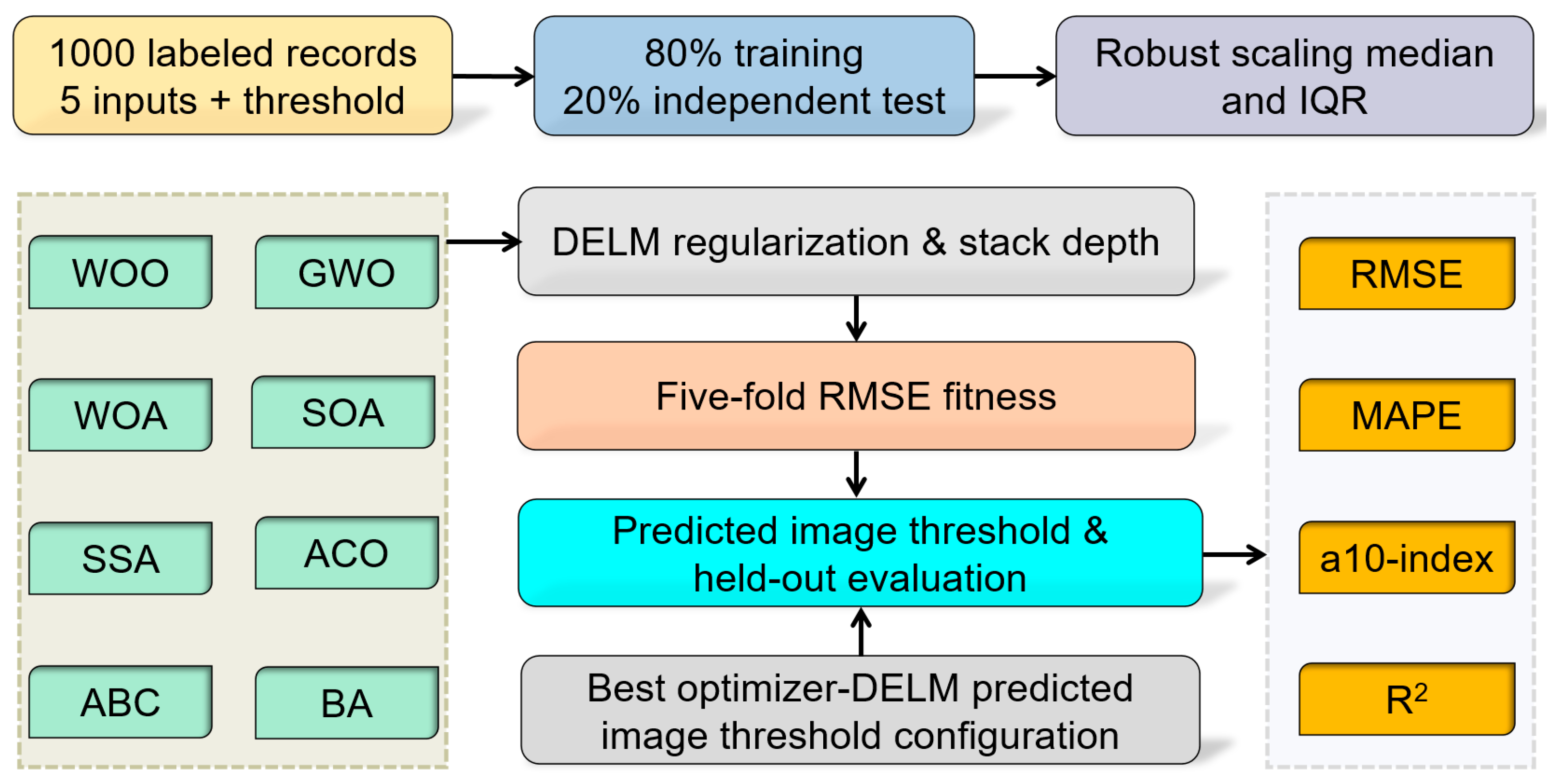
Eight intelligent optimization algorithms are used separately to optimize the DELM regularization coefficient and ELM-AE stacking depth, thereby establishing a nonlinear mapping between the five grayscale statistical features and manually reviewed thresholds. All models use the same data split, parameter search ranges, and fitness function. Hyperparameters are selected using five-fold cross-validation within the training set. The independent test set is reserved for final evaluation and is not used for training or parameter optimization. Figure 9 shows the procedure.

Figure 9. DELM threshold prediction workflow driven by eight optimization algorithms.

(1)

Data splitting. The 800 training records and 200 independent test records established in Section 2.2 are retained; the 1000 records are not pooled and split again. Each source image and its augmented records remain in the same subset. Five-fold cross-validation within the training set groups records by source-image identifier and uses only training records to evaluate candidate parameters. Independent test records are excluded from fold construction and parameter selection.

(2)

Data scaling. Robust scaling is applied to the five input variables using the training-data median as the center and the interquartile range as the scale [58]. During five-fold cross-validation, scaling parameters are calculated from the current training folds only and applied to the corresponding validation fold. After the final model is trained, scaling parameters are calculated from the full training set and then applied to the independent test set.

(3)

Parameter encoding. The regularization coefficient is searched on a logarithmic scale, and the number of stacked ELM-AE layers is restricted to integers. After an optimizer produces a continuous position, the layer count is rounded to the nearest valid integer, and out-of-range values are projected back onto the specified bounds.

(4)

Fitness calculation. The fitness of each candidate parameter combination is the mean RMSE from five-fold cross-validation. All eight algorithms use the same folds, parameter bounds, fitness function, and maximum iteration count. Parameter combinations that cannot be trained are assigned a penalty value. Because the algorithms use different population sizes, however, their numbers of fitness evaluations are not necessarily identical even with the same iteration count. Differences in computational budgets arising from population size should therefore also be considered when comparing prediction errors.

For a candidate (C, L), the hyperparameter-search cost is the mean validation RMSE across the five training-set folds:

$$f(C,L)={\displaystyle \frac{1}{5}}{\displaystyle \sum _{v=1}^5\sqrt{\frac{1}{n_v}{\displaystyle \sum _{i\in V_v}{\left({\widehat{y}}_i^{(-v)}(C,L)-y_i\right)}^2}}}$$

(22)

Here V_v is validation fold v, n_v is its record count, and ŷ_i^(−v)(C,L) is the prediction for record i from a DELM fitted to the other four folds. Lower values of f(C,L) are preferred. The 200 independent test records do not enter this cost; the test-set RMSE, MAPE, R², and a10-index are reported only after parameter selection and refitting on all 800 training records.

(5)

Model training. After the best population size and parameters are determined for each algorithm, the corresponding DELM is rebuilt using all training records, and the training and test metrics are calculated separately.

All eight optimizers were run on the same computing platform in MATLAB R2024b, using the same data partition, five-fold cross-validation objective, hyperparameter bounds, and maximum iteration limit. Population size was selected using the common procedure in Section 5.3. The resulting DELM models were compared using prediction metrics on the common training and test sets.

5.3. Population Size and Parameter Optimization Results

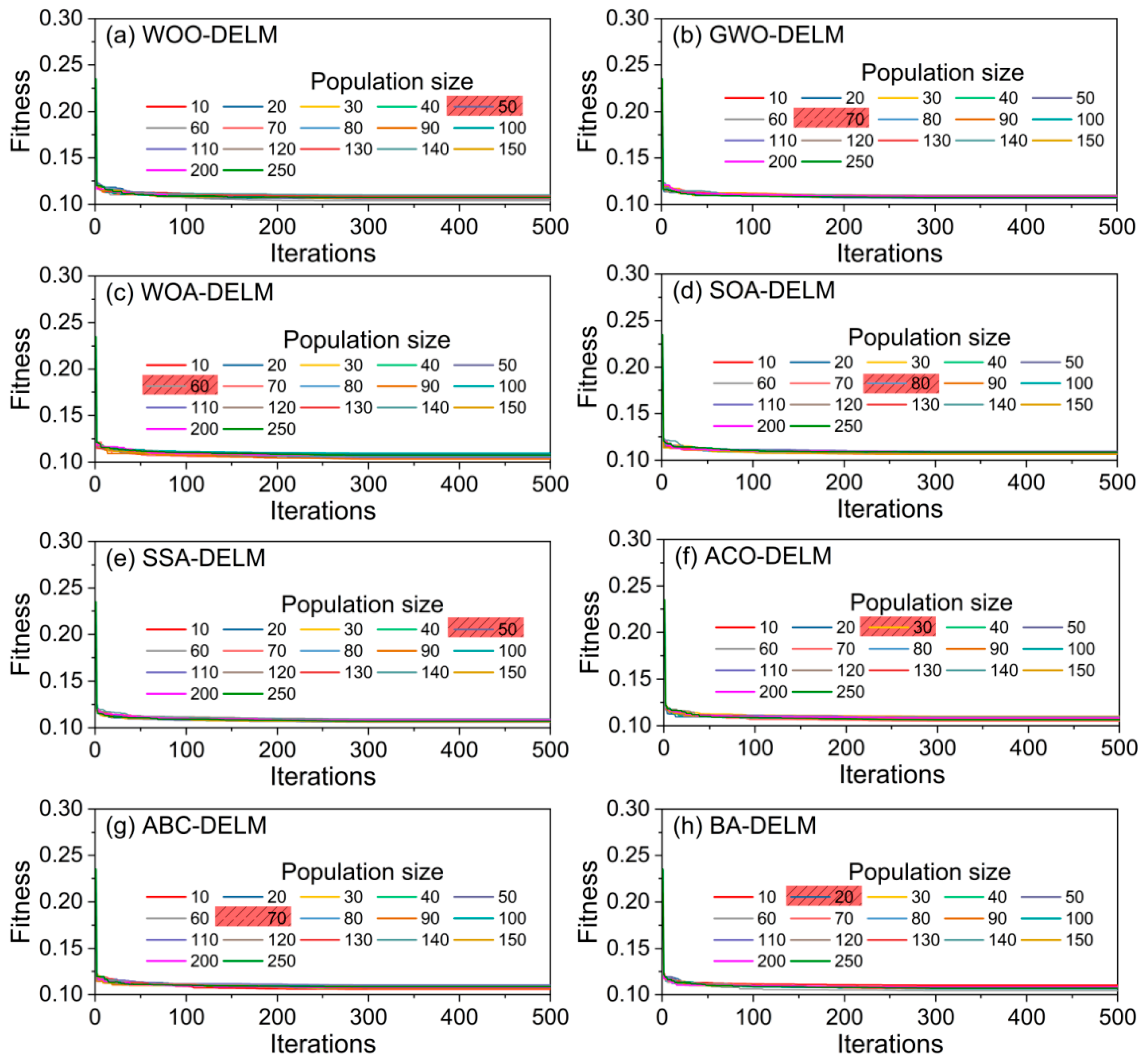
Population size is an important factor affecting the search performance of intelligent optimization algorithms. To determine an appropriate size for each algorithm, candidate population sizes are compared within a common range, and the final value is selected using five-fold cross-validation RMSE. Candidate sizes increase from 10 to 150 in steps of 10, with two additional sizes of 200 and 250. Five-fold validation RMSE is calculated for each size under a fixed iteration count. The results are shown in Figure 10.

Figure 10. RMSE from five-fold cross-validation under eight optimization algorithms: (a) WOO-DELM; (b) GWO-DELM; (c) WOA-DELM; (d) SOA-DELM; (e) SSA-DELM; (f) ACO-DELM; (g) ABC-DELM; (h) BA-DELM.

As shown in Figure 10, the validation RMSE of most algorithms initially decreases and then tends to stabilize as population size increases. Population size therefore affects hyperparameter search, but its benefit does not increase indefinitely. The selected population sizes for GWO, WOA, SOA, SSA, ACO, ABC, BA, and WOO are 70, 60, 80, 50, 30, 70, 20, and 50, respectively. These sizes are used in subsequent hyperparameter searches and performance comparisons of the optimized DELM models.

The selected WOO-DELM has five inputs, three sigmoid ELM-AE layers containing 64, 32, and 16 nodes, and one linear threshold output, with C = 100 and L = 3. C is searched from 0.001 to 1000 on a base-10 logarithmic scale, and integer L is selected from 1 to 4, using the first L widths from 64, 32, 16, and 8. Input weights and biases are sampled from U(−1,1). Base seed 2024 defines a fixed random-parameter bank within each search, while output weights are fitted on the current training fold. The original WOO search uses 50 individuals and at most 500 iterations. Five-fold partitions are grouped by source image, and scaling parameters are fitted within each training fold.

An equal-budget comparison of WOO, grid search, and random search [59] uses 1000 five-fold fitness calls per method. The grid combines 250 logarithmically spaced C values with four L values; random search samples the same log-C interval and integer L set. Twenty independent runs use seeds 1001–1020. Within each run, the folds and DELM random-parameter bank are shared across the three methods, and initialization calls count toward the budget. Test RMSE is summarized by its mean and standard deviation across runs, together with search duration.

Table 1 reports the mean and sample standard deviation of test RMSE and search time over 20 independent runs. Search time covers the complete hyperparameter search, including initialization and all five-fold fitness calculations, but excludes detector training and final refitting on all 800 training records. The three methods use the same timing boundaries and computing environment. In each run, the selected model is refitted before the test RMSE is calculated. The test set is used only for final evaluation and does not guide parameter selection. In this comparison, WOO has the lowest mean test RMSE, whereas grid search has the shortest mean search time.

Table 1. Equal-budget comparison of three hyperparameter search methods over 20 independent runs. Values are means ± sample standard deviations. Each run performs 1000 five-fold fitness evaluations.

Search Method	Fitness Evaluations	Test RMSE	Search Time (s)
WOO	1000	0.0217 ± 0.0011	134.6 ± 8.7
Grid search	1000	0.0220 ± 0.0010	126.8 ± 7.9
Random search	1000	0.0224 ± 0.0013	129.4 ± 8.2

5.4. Comparison of Threshold Prediction Performance

The RMSE, MAPE, R², and a10-index values in this section quantify the accuracy of threshold prediction from the annotated-box features in the threshold dataset. The final crack segmentation is further evaluated at the pixel level in Section 5.5 using IoU, precision, recall, and Dice/F1. Together with the detector evaluation in Section 4, these results describe performance at the localization, threshold-prediction, and final segmentation stages.

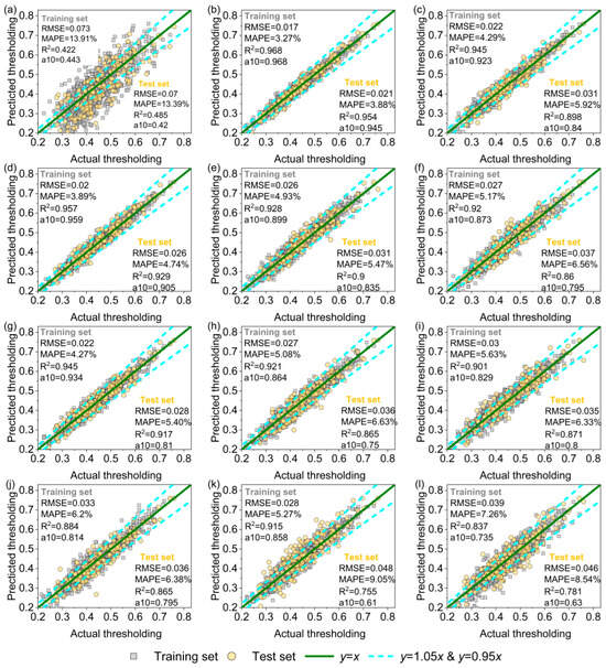
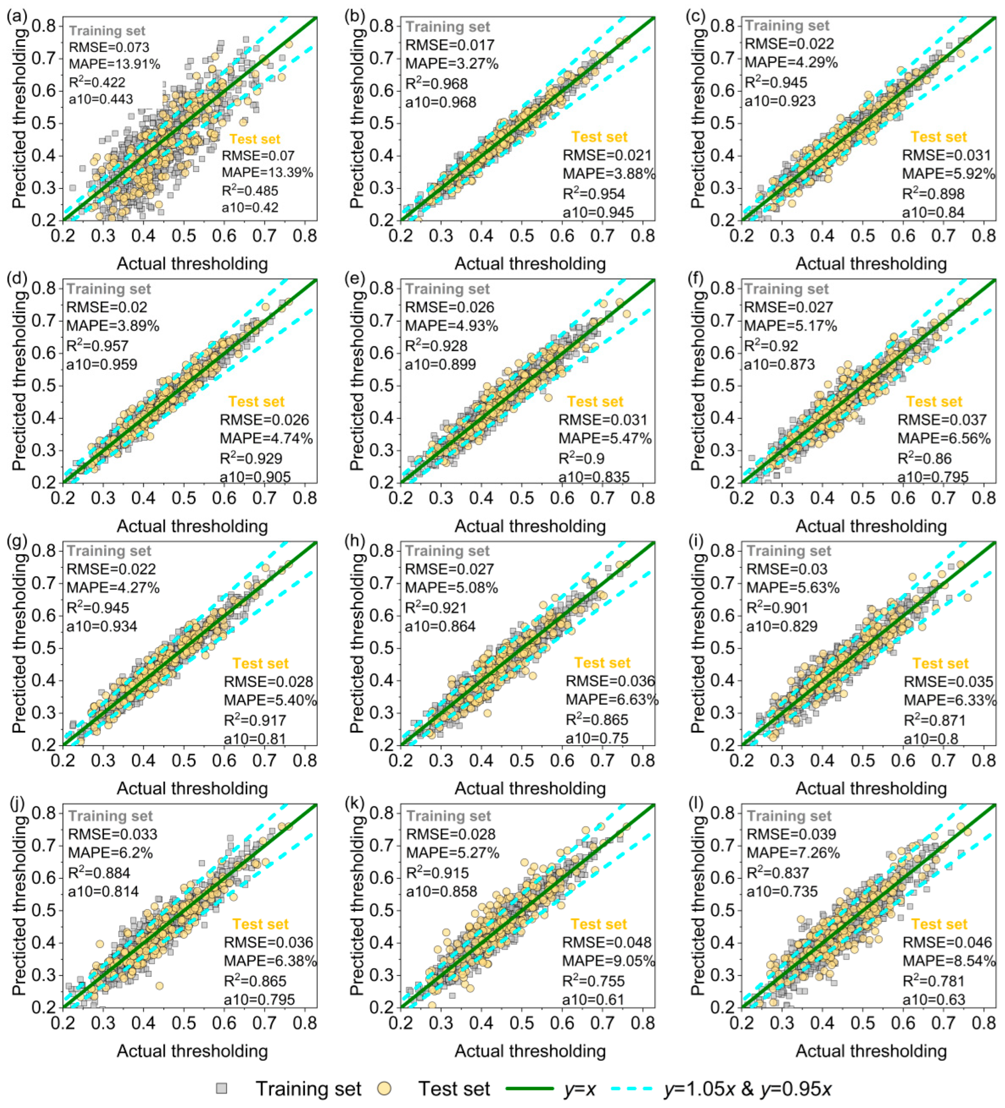
Figure 11 compares the manually reviewed and predicted thresholds of 12 methods on the training and test sets. Scatter points closer to the y = x reference line indicate smaller prediction errors. WOO-DELM achieves an RMSE of 0.017, a MAPE of 3.27%, an R² of 0.968, and an a10-index of 0.968 on the training set. The corresponding test-set metrics are 0.021, 3.88%, 0.954, and 0.945. The training and test results are relatively close, indicating good threshold prediction on the current dataset without a marked imbalance in performance between the two sets. In contrast, Otsu’s method, RF, and BP show more pronounced prediction deviations over some threshold intervals, whereas the scatter points from optimized DELM models generally lie closer to the ideal reference line. Compared with DELM without hyperparameter optimization, optimized DELM models yield lower prediction errors, suggesting that hyperparameter optimization improves their ability to fit the nonlinear relationship between grayscale statistics and segmentation thresholds.

Figure 11. Comparison of observed and predicted thresholds on the training and test sets: (a) Otsu’s method; (b) WOO-DELM; (c) GWO-DELM; (d) WOA-DELM; (e) SOA-DELM; (f) SSA-DELM; (g) ACO-DELM; (h) ABC-DELM; (i) BA-DELM; (j) DELM; (k) RF; (l) BP.

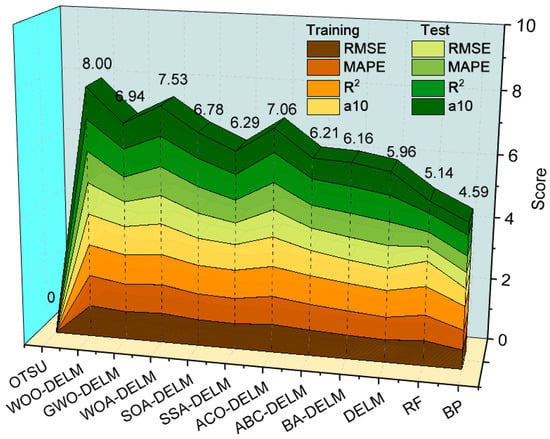
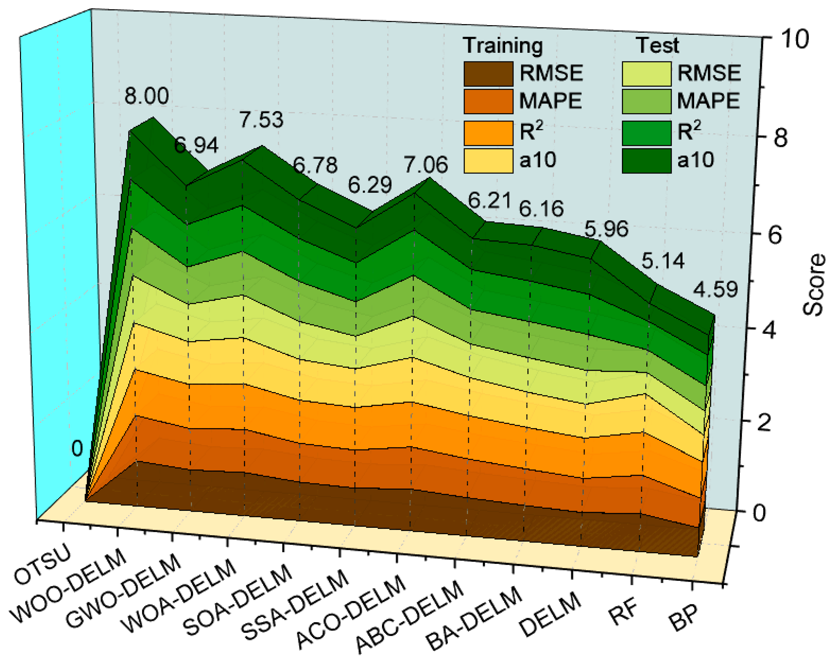
Figure 12 summarizes relative threshold-prediction performance using an equally weighted composite score. Let E(m,d,q) denote metric q for model m on dataset d, where d is the training or test set. For each dataset and metric separately, E(min,d,q) and E(max,d,q) denote the minimum and maximum across the 12 comparison models. These quantities are written with subscripts in Equations (23)–(25). For the two error metrics, the normalized score is

$$s_{m,d,q}={\displaystyle \frac{E_{\max ,d,q}-E_{m,d,q}}{E_{\max ,d,q}-E_{\min ,d,q}}}, q\in \left\{\mathrm{RMSE},\mathrm{MAPE}\right\}$$

(23)

Figure 12. Relative composite threshold-prediction scores for 12 models, with equal weights for four metrics on each of the training and test sets.

For the two agreement metrics, the normalized score is

$$s_{m,d,q}={\displaystyle \frac{E_{m,d,q}-E_{\min ,d,q}}{E_{\max ,d,q}-E_{\min ,d,q}}}, q\in \left\{R^2,\mathrm{a}10\right\}$$

(24)

The composite score is the sum of the four normalized metrics on each of the two datasets:

$$Q_m={\displaystyle \sum _{d\in \left\{\mathrm{train},\mathrm{test}\right\}}{\displaystyle \sum _{q\in \left\{\mathrm{RMSE},\mathrm{MAPE},R^2,\mathrm{a}10\right\}}{s}_{m,d,q}}}$$

(25)

Each component lies between 0 and 1, so the eight equally weighted components give a score between 0 and 8. Figure 12 reports 8.00 for WOO-DELM, 7.53 for WOA-DELM, and 0.00 for Otsu’s method. These values depend on the comparison models and the extrema used for normalization. A score of 8.00 means that a model has the most favorable reported values in these eight columns; it is not a 100% segmentation accuracy. The score includes training performance and is interpreted together with the separate held-out threshold metrics in Figure 11. It is not an absolute measure of pixel-level segmentation accuracy or performance in other tunnels.

A paired comparison is performed on the same 200 independent threshold test images to quantify the effect of replacing manually annotated regions with detected regions. In Case A, AGIF, AGIB, SDIF, SDIB, and EDIR are calculated from manually annotated boxes; in Case B, the same features are calculated from Faster R-CNN-predicted boxes. Overlapping boxes are merged, predicted coordinates are mapped back to the original image, and the foreground and background are then defined as in Section 2.2. Both cases use the same trained WOO-DELM model, the robust scaler determined from the training data, and the manually reviewed reference thresholds. C = 100, L = 3, all fitted weights, and the detector settings remain fixed. Neither Faster R-CNN nor DELM is retrained for this comparison.

Table 2 reports the paired threshold-prediction results. With manually annotated boxes, RMSE, MAPE, R², and a10-index are 0.021, 3.88%, 0.954, and 0.945, respectively. With predicted boxes, the corresponding values are 0.023, 4.26%, 0.945, and 0.930. Under these paired conditions with the model fixed, RMSE increases by 0.002, quantifying the change in threshold prediction caused by changing the source of the bounding boxes.

Table 2. Paired comparison of threshold prediction using manually annotated and detector-predicted boxes on the same 200 independent test images, with the trained WOO-DELM model held fixed.

Feature Source	RMSE	MAPE (%)	R2	a10-Index
Case A: annotated boxes	0.021	3.88	0.954	0.945
Case B: predicted boxes	0.023	4.26	0.945	0.930

5.5. Quantitative Evaluation of Crack Segmentation

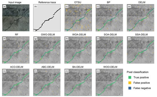
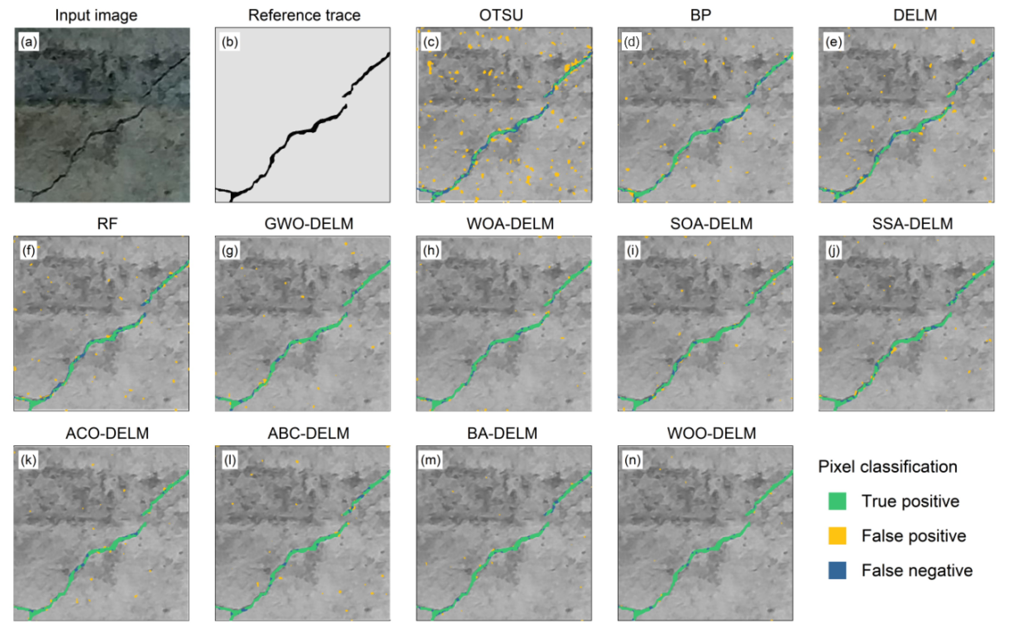
The final segmentation results of the Faster R-CNN–WOO-DELM framework are evaluated in this section. Figure 13 compares the extracted crack traces with the manually corrected reference, focusing on crack continuity, fine-branch retention, and background interference. Figure 14 reports the image-level means and standard deviations of the segmentation metrics for Otsu thresholding and for segmentations obtained using thresholds predicted by BP, RF, DELM, and eight optimizer–DELM configurations.

Figure 13. Pixel-wise visual comparison of crack segmentation results: (a) input image; (b) manually corrected reference; (c) Otsu; (d) BP; (e) DELM; (f) RF; (g) GWO-DELM; (h) WOA-DELM; (i) SOA-DELM; (j) SSA-DELM; (k) ACO-DELM; (l) ABC-DELM; (m) BA-DELM; and (n) WOO-DELM.

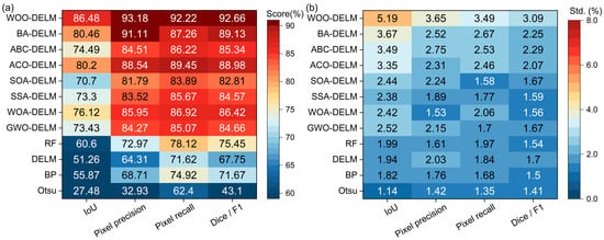
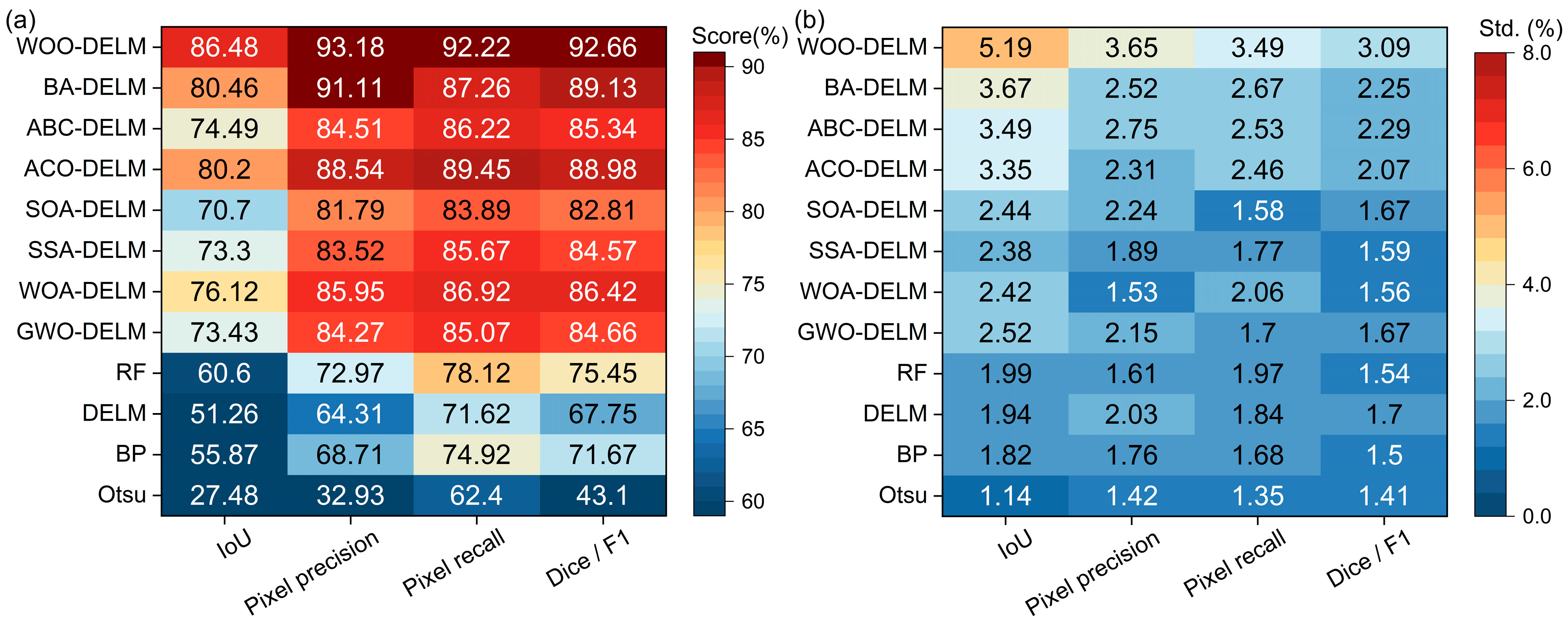
Figure 14. Pixel-level segmentation performance on 30 independent test images: (a) image-level means of the metrics; (b) corresponding sample standard deviations. Means are expressed as percentages and standard deviations as percentage points.

Thirty independent test images are selected from the independent detector test set for pixel-level segmentation evaluation, retaining only one image for each source-image identifier. Based on the dominant imaging conditions, the images are divided into three nonoverlapping groups: relatively uniform illumination with clear crack contrast; uneven illumination or local shadows; and complex or wet textures with low crack contrast. Each group contains 10 images. All 12 methods are evaluated on the same 30 images. The reference mask for every evaluated image is individually corrected at the pixel level after threshold-based initialization. The corrected reference for each image is held fixed across methods.

IoU, pixel precision, pixel recall, and Dice/F1 are calculated separately for each image using the definitions in Section 4. The reported mean is the unweighted arithmetic mean of the 30 image-level values. The standard deviation is the sample standard deviation across these images, calculated with a denominator of 29. The three groups describe the composition of the test subset and are not treated as three independent measurements. Pixel counts are not pooled across images before calculating the reported metrics. Figure 14a presents the image-level means, and Figure 14b presents the corresponding sample standard deviations. Means are expressed as percentages and standard deviations as percentage points.

Figure 13a presents the input tunnel-lining image, Figure 13b presents the reference trace, and Figure 13c–n presents the segmentation overlays for the 12 methods. Green indicates pixels shared by the predicted and reference masks; orange indicates additional pixels, and blue indicates missing pixels relative to the reference mask. The extent of the green trace shows how much of the reference crack is retained, while the locations of orange and blue pixels reveal background inclusion and local omissions. Otsu thresholding produces numerous additional pixels in textured background regions. BP, RF, and DELM reduce this interference, but local omissions remain along portions of the crack. The optimized DELM models retain more of the main trace, with differences in the preservation of fine details and suppression of scattered background pixels. In Figure 13n, WOO-DELM follows the reference main crack closely, retains the visible fine branches, and produces few additional or missing pixels. These spatial details show the final segmentation behavior beyond the location and extent represented by bounding boxes.

As shown in Figure 14, WOO-DELM achieves an IoU of 86.48 ± 5.19%, pixel precision of 93.18 ± 3.65%, pixel recall of 92.22 ± 3.49%, and Dice/F1 of 92.66 ± 3.09% across the 30 test images. Figure 13 further illustrates these image-level statistics through spatial comparisons of a representative image.

Among the other optimized DELM methods, BA-DELM achieves an IoU of 80.46 ± 3.67% and Dice/F1 of 89.13 ± 2.25%. WOO-DELM exceeds these mean IoU and Dice/F1 values by 6.02 and 3.53 percentage points, respectively. WOO-DELM has the highest mean scores and the largest standard deviations, indicating greater variation across the evaluated images.

In the automated workflow, the final binary crack map is produced from detector-defined regions through grayscale feature extraction, threshold prediction, binarization, and post-processing. Evaluation of the final crack pixels therefore reflects the combined effects of these stages, including the influence of the initial localization on the subsequent segmentation. The detector assessment in Section 4 and the final pixel assessment address successive stages of the same workflow, with the final segmentation serving as the application output.

6. Sensitivity Analysis

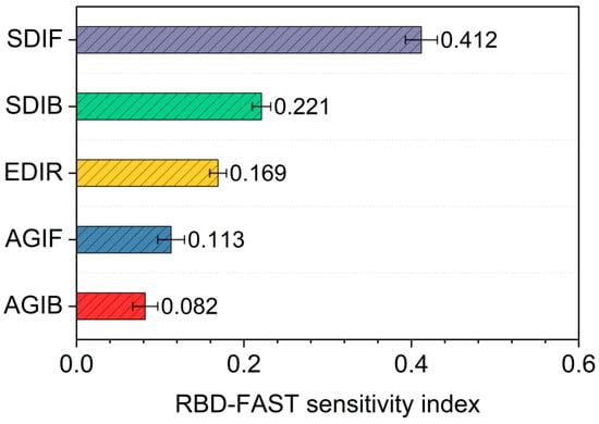
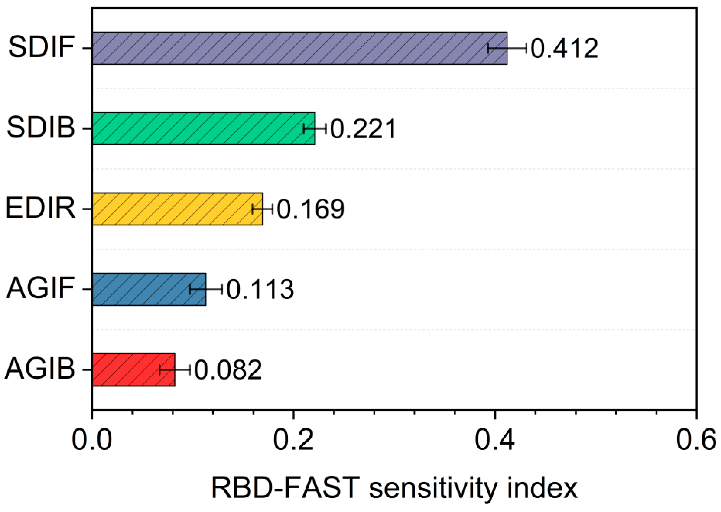
Random balance design–Fourier amplitude sensitivity testing (RBD-FAST) is used to evaluate the relative influence of the five grayscale features on the fitted WOO-DELM threshold predictor [60,61]. The analysis uses 1024 samples per run and 20 independent random permutations, with the trained model parameters fixed; the reported first-order indices are the means of the 20 calculations. For 8-bit images, the sampling ranges are 0–255 for AGIF, AGIB, and EDIR and 0–127.5 for SDIF and SDIB. Division by the respective upper bounds expresses the sampling domain on a 0–1 scale; sampled features are converted to model inputs using the training-derived robust scaler in Section 5.2. The first-order sensitivity index is calculated using Equation (26):

$$S_i={\displaystyle \frac{a_i^2+b_i^2}{{\displaystyle \sum _{k=1}^n(a_k^2+b_k^2)}}}$$

(26)

where S_i is the first-order sensitivity index of input variable i, and ai and bi are the Fourier cosine and sine coefficients at the corresponding frequency. The numerator represents output variance attributable to the variable, and the denominator is the total variance of the frequency components considered. Figure 15 reports the mean first-order sensitivity indices from 20 random permutations.

Figure 15. RBD-FAST sensitivity indices of five image statistical features.

The analysis considers the inputs independently within the specified sampling ranges. Under this assumption, the first-order indices compare the contributions of individual features to variation in the predicted threshold and provide a relative feature-influence ranking for the fitted model under the stated sampling conditions.

Figure 15 gives first-order indices of 0.412, 0.221, 0.169, 0.113, and 0.082 for SDIF, SDIB, EDIR, AGIF, and AGIB, respectively. SDIF has the greatest influence under the specified analysis conditions, followed by SDIB. This result complements the observed correlation of approximately 0.74 between SDIF and the reviewed reference threshold in Figure 3 and supports the relevance of grayscale dispersion to threshold prediction.

7. Limitations

The model was trained and evaluated using an existing tunnel lining crack dataset and its augmented images. Although the source images were collected from actual tunnel environments, the reported performance is limited to the current dataset, and generalization across different tunnels and imaging conditions has not yet been independently verified. Differences in lining materials, seepage conditions, ancillary facilities, curved-surface perspective, camera distortion, and motion blur may affect the distributions of detection boxes and grayscale statistical features. Further validation using images from different tunnels and inspection conditions is therefore necessary.

In addition, although pixel-level segmentation was quantitatively evaluated using 30 independent test images, a systematic assessment across the complete test set using independent pixel-level annotations has not yet been performed. The current results support the effectiveness of the proposed framework in threshold prediction and crack segmentation under the investigated conditions, while its performance in more complex engineering environments requires further validation.

Furthermore, manually reviewed thresholds are used as supervised learning labels. Threshold selection considers crack connectivity, retention of fine branches, and background suppression, but annotators may differ in their tolerance of fine branches and background noise. For low-contrast cracks or complex textured backgrounds, different thresholds may yield similar segmentation results, so a manually determined reference threshold is not necessarily uniquely optimal. Future work could incorporate inter-annotator agreement analysis, independent pixel-level reference annotations, and objective segmentation criteria to improve the reliability of reference thresholds.

8. Conclusions

To address the insufficient integration of crack localization and adaptive segmentation in tunnel linings under complex background conditions, this study developed an integrated Faster R-CNN-WOO-DELM framework and examined crack detection, threshold prediction, and final segmentation behavior through model comparisons and sensitivity analysis. The main conclusions are as follows.

(1)

Faster R-CNN effectively locates candidate crack regions, providing a basis for subsequent grayscale feature extraction and adaptive threshold prediction. At a confidence threshold of 0.45, precision and recall are 79.2% and 93.1%, respectively, with an F1 score of approximately 0.856 and an AP of 0.874. The method retains most crack targets, although some low-contrast cracks and regions with complex backgrounds remain subject to missed and false detections.

(2)

WOO-DELM predicts the manually reviewed thresholds from annotated-box features, achieving an RMSE of 0.021, a MAPE of 3.88%, an R² of 0.954, and an a10-index of 0.945 on the held-out threshold test set. Across 30 independent test images, WOO-DELM achieves image-level IoU, precision, recall, and Dice/F1 values of 86.48 ± 5.19%, 93.18 ± 3.65%, 92.22 ± 3.49%, and 92.66 ± 3.09%, respectively, expressed as means ± sample standard deviations. These results support the use of WOO-DELM for adaptive threshold prediction and crack extraction.

(3)

RBD-FAST gives first-order sensitivity indices of 0.412, 0.221, 0.169, 0.113, and 0.082 for SDIF, SDIB, EDIR, AGIF, and AGIB, respectively. Under the specified sampling conditions and independent-input assumption, SDIF has the greatest influence on the fitted model’s predicted threshold, followed by SDIB. These results help explain the role of regional grayscale dispersion in adaptive threshold prediction.

References

- Yin, Z.; Lei, Z.; Zheng, A.; Zhu, J.; Liu, X.-Z. Automatic detection and association analysis of multiple surface defects on shield subway tunnels. Sensors 2023, 23, 7106. [Google Scholar] [CrossRef] [Scilit] [PubMed]
- Huang, H.; Li, Q.; Zhang, D. Deep learning based image recognition for crack and leakage defects of metro shield tunnel. Tunn. Undergr. Space Technol. 2018, 77, 166–176. [Google Scholar] [CrossRef] [Scilit]
- Xue, Y.; Li, Y. A fast detection method via region-based fully convolutional neural networks for shield tunnel lining defects. Comput. Aided Civil. Infrastruct. Eng. 2018, 33, 638–654. [Google Scholar] [CrossRef] [Scilit]
- Xue, Y.; Cai, X.; Shadabfar, M.; Shao, H.; Zhang, S. Deep learning-based automatic recognition of water leakage area in shield tunnel lining. Tunn. Undergr. Space Technol. 2020, 104, 103524. [Google Scholar] [CrossRef] [Scilit]
- Man, K.; Liu, R.; Liu, X.; Song, Z.; Liu, Z.; Cao, Z.; Wu, L. Water leakage and crack identification in tunnels based on transfer-learning and convolutional neural networks. Water 2022, 14, 1462. [Google Scholar] [CrossRef] [Scilit]
- Zhou, Z.; Zhang, J.; Gong, C.; Wu, W. Automatic tunnel lining crack detection via deep learning with generative adversarial network-based data augmentation. Undergr. Space 2023, 9, 140–154. [Google Scholar] [CrossRef] [Scilit]
- Zhou, Z.; Zhang, J.; Gong, C. Automatic detection method of tunnel lining multi-defects via an enhanced You Only Look Once network. Comput. Aided Civil. Infrastruct. Eng. 2022, 37, 762–780. [Google Scholar] [CrossRef] [Scilit]
- Liu, J.; Zhao, Z.; Lv, C.; Ding, Y.; Chang, H.; Xie, Q. An image enhancement algorithm to improve road tunnel crack transfer detection. Constr. Build. Mater. 2022, 348, 128583. [Google Scholar] [CrossRef] [Scilit]
- Huang, Z.; Fu, H.; Chen, W.; Zhang, J.; Huang, H. Damage detection and quantitative analysis of shield tunnel structure. Autom. Constr. 2018, 94, 303–316. [Google Scholar] [CrossRef] [Scilit]
- Li, G.; Ma, B.; He, S.; Ren, X.; Liu, Q. Automatic tunnel crack detection based on U-Net and a convolutional neural network with alternately updated clique. Sensors 2020, 20, 717. [Google Scholar] [CrossRef] [Scilit] [PubMed]
- Jiang, Y.; Wang, L.; Zhang, B.; Dai, X.; Ye, J.; Sun, B.; Liu, N.; Wang, Z.; Zhao, Y. Tunnel lining detection and retrofitting. Autom. Constr. 2023, 152, 104881. [Google Scholar] [CrossRef] [Scilit]
- Feng, S.J.; Feng, Y.; Zhang, X.L.; Chen, Y.H. Deep learning with visual explanations for leakage defect segmentation of metro shield tunnel. Tunn. Undergr. Space Technol. 2023, 136, 105107. [Google Scholar] [CrossRef] [Scilit]
- Feng, Y.; Feng, S.J.; Zhang, X.L.; Zhang, D.-M.; Zhao, Y. A two-step deep learning-based framework for metro tunnel lining defect recognition. Tunn. Undergr. Space Technol. 2024, 150, 105832. [Google Scholar] [CrossRef] [Scilit]
- Lei, M.; Liu, L.; Shi, C.; Tan, Y.; Lin, Y.; Wang, W. A novel tunnel-lining crack recognition system based on digital image technology. Tunn. Undergr. Space Technol. 2021, 108, 103724. [Google Scholar] [CrossRef] [Scilit]
- Zhou, Z.; Yan, L.; Zhang, J.; Zheng, Y.; Gong, C.; Yang, H.; Deng, E. Automatic segmentation of tunnel lining defects based on multiscale attention and context information enhancement. Constr. Build. Mater. 2023, 387, 131621. [Google Scholar] [CrossRef] [Scilit]
- Feng, Y.; Zhang, X.; Feng, S.; Chen, H.; Zhao, Y.; Chen, Y. Improved SOLOv2 detection method for shield tunnel lining water leakages. J. Intell. Constr. 2023, 1, 9180004. [Google Scholar] [CrossRef] [Scilit]
- Zhang, X.; Lin, X.; Zhang, W.; Feng, Y.; Lan, W.; Da, Y.; Hu, K. Intelligent recognition of voids behind tunnel linings using deep learning and percussion sound. J. Intell. Constr. 2023, 1, 9180029. [Google Scholar] [CrossRef] [Scilit]
- Ouyang, A.; Di Murro, V.; Cull, M.; Cunningham, R.; Osborne, J.A.; Li, Z. Automated pixel-level crack monitoring system for large-scale underground infrastructure—A case study at CERN. Tunn. Undergr. Space Technol. 2023, 140, 105310. [Google Scholar] [CrossRef] [Scilit]
- Wang, H.; Li, Y.; Dang, L.M.; Lee, S.; Moon, H. Pixel-level tunnel crack segmentation using a weakly supervised annotation approach. Comput. Ind. 2021, 133, 103545. [Google Scholar] [CrossRef] [Scilit]
- Li, D.; Xie, Q.; Gong, X.; Yu, Z.; Xu, J.; Sun, Y.; Wang, J. Automatic defect detection of metro tunnel surfaces using a vision-based inspection system. Adv. Eng. Inform. 2021, 47, 101206. [Google Scholar] [CrossRef] [Scilit]
- Miao, X.; Wang, J.; Wang, Z.; Sui, Q.; Gao, Y.; Jiang, P. Automatic recognition of highway tunnel defects based on an improved U-net model. IEEE Sens. J. 2019, 19, 11413–11423. [Google Scholar] [CrossRef] [Scilit]
- Dang, L.M.; Wang, H.; Li, Y.; Park, Y.; Oh, C.; Nguyen, T.N.; Moon, H. Automatic tunnel lining crack evaluation and measurement using deep learning. Tunn. Undergr. Space Technol. 2022, 124, 104472. [Google Scholar] [CrossRef] [Scilit]
- Song, Q.; Wu, Y.; Xin, X.; Yang, L.; Yang, M.; Chen, H.; Liu, C.; Hu, M.; Chai, X.; Li, J. Real-time tunnel crack analysis system via deep learning. IEEE Access 2019, 7, 64186–64197. [Google Scholar] [CrossRef] [Scilit]
- Xu, L.; Wang, Y.; Dong, A.; Zhu, L.; Shi, H.; Yu, Z. Image-based intelligent detection of typical defects of complex subway tunnel surface. Tunn. Undergr. Space Technol. 2023, 140, 105266. [Google Scholar] [CrossRef] [Scilit]
- Zhao, S.; Zhang, D.; Xue, Y.; Zhou, M.; Huang, H. A deep learning-based approach for refined crack evaluation from shield tunnel lining images. Autom. Constr. 2021, 132, 103934. [Google Scholar] [CrossRef] [Scilit]
- Xu, Y.; Li, D.; Xie, Q.; Wu, Q.; Wang, J. Automatic defect detection and segmentation of tunnel surface using modified Mask R-CNN. Measurement 2021, 178, 109316. [Google Scholar] [CrossRef] [Scilit]
- Kang, D.; Benipal, S.S.; Gopal, D.L.; Cha, Y.-J. Hybrid pixel-level concrete crack segmentation and quantification across complex backgrounds using deep learning. Autom. Constr. 2020, 118, 103291. [Google Scholar] [CrossRef] [Scilit]
- Cha, Y.; Choi, W.; Büyüköztürk, O. Deep learning-based crack damage detection using convolutional neural networks. Comput. Aided Civil. Infrastruct. Eng. 2017, 32, 361–378. [Google Scholar] [CrossRef] [Scilit]
- Ren, Y.; Huang, J.; Hong, Z.; Lu, W.; Yin, J.; Zou, L.; Shen, X. Image-based concrete crack detection in tunnels using deep fully convolutional networks. Constr. Build. Mater. 2020, 234, 117367. [Google Scholar] [CrossRef] [Scilit]
- Feng, Y.; Feng, S.J.; Zhang, X.L.; Zhang, W.; Hu, K.; Da, Y.-W. Intelligent segmentation and quantification of tunnel lining cracks via computer vision. Struct. Health Monit. 2025, 24, 1896–1926. [Google Scholar] [CrossRef] [Scilit]
- Lazaridis, P.C.; Thomoglou, A.K. Rapid shear capacity prediction of TRM-strengthened unreinforced masonry walls through interpretable machine learning deployed in a web app. J. Build. Eng. 2024, 98, 110912. [Google Scholar] [CrossRef] [Scilit]
- Gray, D.T.; Simwanda, L.; Sifan, M.; Poologanathan, K.; Kannan, T. Machine learning prediction of shear strength in cold-formed steel modular construction-optimised (MCO) beam. Buildings 2026, 16, 1497. [Google Scholar] [CrossRef] [Scilit]
- Tzutalin. LabelImg. Git Code 2015. Available online: https://github.com/tzutalin/labelImg (accessed on 13 October 2026).
- LeCun, Y.; Bottou, L.; Bengio, Y.; Haffner, P. Gradient-based learning applied to document recognition. Proc. IEEE 1998, 86, 2278–2324. [Google Scholar] [CrossRef] [Scilit]
- Ren, S.; He, K.; Girshick, R.; Sun, J. Faster R-CNN: Towards real-time object detection with region proposal networks. IEEE Trans. Pattern Anal. Mach. Intell. 2017, 39, 1137–1149. [Google Scholar] [CrossRef] [Scilit] [PubMed]
- He, K.; Zhang, X.; Ren, S.; Sun, J. Deep residual learning for image recognition. Proc. IEEE Conf. Comput. Vis. Pattern Recognit. 2016, 770–778. [Google Scholar] [CrossRef] [Scilit]
- Canny, J. A computational approach to edge detection. IEEE Trans. Pattern Anal. Mach. Intell. 1986, 8, 679–698. [Google Scholar] [CrossRef] [Scilit]
- Ronneberger, O.; Fischer, P.; Brox, T. U-Net: Convolutional networks for biomedical image segmentation. In MICCAI 2015; Springer: Cham, Switzerland, 2015; pp. 234–241. [Google Scholar]
- Chen, L.C.; Zhu, Y.; Papandreou, G.; Schroff, F.; Adam, H. Encoder-decoder with atrous separable convolution for semantic image segmentation. In ECCV 2018; Springer: Cham, Switzerland, 2018; pp. 801–818. [Google Scholar]
- Peng, Y.; Gu, S.; Liang, Y.; Ouyang, K.; Li, Y.; Wang, K.; Wu, G.; Fan, C. Wave Optics Optimizer: A novel meta-heuristic algorithm for engineering optimization. Commun. Nonlinear Sci. Numer. Simul. 2025, 152, 109337. [Google Scholar] [CrossRef] [Scilit]
- Huang, G.B.; Zhu, Q.Y.; Siew, C.K. Extreme learning machine: Theory and applications. Neurocomputing 2006, 70, 489–501. [Google Scholar] [CrossRef] [Scilit]
- Kasun, L.L.C.; Zhou, H.; Huang, G.B.; Vong, C.M. Representation learning with extreme learning machines for big data. IEEE Intell. Syst. 2013, 28, 31–34. [Google Scholar]
- Ding, S.; Zhao, H.; Zhang, Y.; Xu, X.; Nie, R. Extreme learning machine: Algorithm, theory and applications. Artif. Intell. Rev. 2015, 44, 103–115. [Google Scholar] [CrossRef] [Scilit]
- Zhou, S.; Lei, Y.; Zhang, Z.X.; Luo, X.; Meng, X. Lightweight evaluation to uniaxial compressive strength of rock by nondestructive characteristic impedance and explainable data-driven techniques. Nondestruct. Test. Eval. 2026, 41, 7730–7760. [Google Scholar] [CrossRef] [Scilit]
- The MathWorks, Inc. MATLAB Documentation. Available online: https://www.mathworks.com/help/matlab/ (accessed on 14 October 2026).
- The MathWorks, Inc. Object Detection Using Faster R-CNN Deep Learning. Available online: https://www.mathworks.com/help/vision/ug/object-detection-using-faster-r-cnn-deep-learning.html (accessed on 14 October 2026).
- Powers, D.M.W. Evaluation: From precision, recall and F-measure to ROC, informedness, markedness and correlation. J. Mach. Learn. Technol. 2011, 2, 37–63. [Google Scholar]
- Mirjalili, S.; Mirjalili, S.M.; Lewis, A. Grey Wolf Optimizer. Adv. Eng. Softw. 2014, 69, 46–61. [Google Scholar] [CrossRef] [Scilit]
- Mirjalili, S.; Lewis, A. The Whale Optimization Algorithm. Adv. Eng. Softw. 2016, 95, 51–67. [Google Scholar] [CrossRef] [Scilit]
- Dhiman, G.; Kumar, V. Seagull optimization algorithm: Theory and its applications for large-scale industrial engineering problems. Knowl. Based Syst. 2019, 165, 169–196. [Google Scholar] [CrossRef] [Scilit]
- Xue, J.; Shen, B. A novel swarm intelligence optimization approach: Sparrow search algorithm. Syst. Sci. Control Eng. 2020, 8, 22–34. [Google Scholar] [CrossRef] [Scilit]
- Dorigo, M.; Maniezzo, V.; Colorni, A. Ant system: Optimization by a colony of cooperating agents. IEEE Trans. Syst. Man Cybern. B 1996, 26, 29–41. [Google Scholar] [CrossRef] [Scilit] [PubMed]
- Karaboga, D.; Basturk, B. A powerful and efficient algorithm for numerical function optimization: Artificial bee colony algorithm. J. Glob. Optim. 2007, 39, 459–471. [Google Scholar] [CrossRef] [Scilit]
- Yang, X.S. A new metaheuristic bat-inspired algorithm. In Nature Inspired Cooperative Strategies for Optimization; Springer: Berlin/Heidelberg, Germany, 2010; pp. 65–74. [Google Scholar]
- Lei, Y.; Zhou, S.; Luo, X.; Niu, S.; Jiang, N. A comparative study of six hybrid prediction models for uniaxial compressive strength of rock based on swarm intelligence optimization algorithms. Front. Earth Sci. 2022, 10, 930130. [Google Scholar] [CrossRef] [Scilit]
- Zhou, S.; Zhang, Z.X.; Luo, X.; Huang, Y.; Yu, Z.; Yang, X. Predicting dynamic compressive strength of frozen-thawed rocks by characteristic impedance and data-driven methods. J. Rock. Mech. Geotech. Eng. 2024, 16, 2591–2606. [Google Scholar] [CrossRef] [Scilit]
- Otsu, N. A threshold selection method from gray-level histograms. IEEE Trans. Syst. Man Cybern. 1979, 9, 62–66. [Google Scholar] [CrossRef] [Scilit]
- Rousseeuw, P.J.; Croux, C. Alternatives to the median absolute deviation. J. Am. Stat. Assoc. 1993, 88, 1273–1283. [Google Scholar] [CrossRef]
- Bergstra, J.; Bengio, Y. Random Search for Hyper-Parameter Optimization. J. Mach. Learn. Res. 2012, 13, 281–305. Available online: https://www.jmlr.org/papers/v13/bergstra12a.html (accessed on 18 June 2026).
- Tarantola, S.; Gatelli, D.; Mara, T.A. Random balance designs for the estimation of first order global sensitivity indices. Reliab. Eng. Syst. Saf. 2006, 91, 717–727. [Google Scholar] [CrossRef] [Scilit]
- Saltelli, A.; Ratto, M.; Andres, T.; Campolongo, F.; Cariboni, J.; Gatelli, D.; Saisana, M.; Tarantola, S. Global Sensitivity Analysis: The Primer; Wiley: Chichester, UK, 2008. [Google Scholar]
Disclaimer/Publisher’s Note: The statements, opinions and data contained in all publications are solely those of the individual author(s) and contributor(s) and not of MDPI and/or the editor(s). MDPI and/or the editor(s) disclaim responsibility for any injury to people or property resulting from any ideas, methods, instructions or products referred to in the content. |
© 2026 by the authors. Licensee MDPI, Basel, Switzerland. This article is an open access article distributed under the terms and conditions of the Creative Commons Attribution (CC BY) license.