


Abstract
Accurate estimation of wind loads is essential for the structural design and performance assessment of long-span curved roofs, which are highly susceptible to wind pressures. However, the number of pressure taps typically used in wind tunnel tests is limited, and conventional interpolation and reconstruction methods may not adequately capture the non-uniform spatial dependencies of wind pressures, particularly in regions affected by flow separation and pronounced roof curvature. To address this issue, this study proposes a hybrid reconstruction framework that integrates Proper Orthogonal Decomposition (POD) with a Graph Attention Network (GAT) to estimate wind pressures at unmeasured locations on long-span curved roofs, including pressure coefficients, pressure time histories, and spectral characteristics. POD is performed independently for each wind direction. For a representative wind direction, the first 50 modes are retained, capturing 96.7% of the fluctuating-pressure energy. Subsequently, a spatial graph is constructed according to the arrangement of the pressure taps, and the GAT is used to adaptively learn the spatial correlations among the taps. This enables the reconstruction of wind-pressure fields under sparse measurement conditions. Across the evaluated cases, the proposed POD–GAT model achieves R2 values exceeding 0.90 for both the mean and fluctuating pressure coefficients. In critical regions characterized by severe flow separation and pronounced surface curvature, the reconstruction based on the POD modal coefficients predicted by the GAT generally yields smaller absolute errors than those obtained using radial basis function (RBF), convolutional neural network (CNN), and multilayer perceptron (MLP) models. In addition, the reconstructed power spectral densities agree well with the experimental results, with only a minor loss of high-frequency energy. The model also maintains stable prediction accuracy for wind directions of 0°, 45°, and 90°. Overall, the proposed method effectively captures complex spatial dependencies while maintaining computational efficiency, thereby providing a reliable approach for refined wind-pressure reconstruction and wind-load assessment of long-span curved roofs.
1. Introduction
Long-span roof structures are widely adopted in large public buildings, such as stadiums, airport terminals, and exhibition centers, because they can provide large enclosed spaces without internal columns [1,2]. These structures are typically characterized by light weight, large span, low damping, and low fundamental frequency, and are therefore highly sensitive to wind effects. In particular, wind pressures in windward edge and roof corner regions often exhibit pronounced non-Gaussian characteristics [3]. Accurate characterization of wind pressure is therefore essential for the wind-resistant design and refined wind load assessment of long-span roof structures.
Over the past decade, wind load data have mainly been obtained from wind tunnel testing and computational fluid dynamics (CFD) simulations [4,5]. Owing to their lower cost than full-scale measurements and greater reliability than CFD simulations in many engineering applications, wind tunnel tests remain the dominant approach for acquiring wind load data. With the development of synchronous pressure acquisition systems based on pressure scanning valves, more than 1000 pressure taps can now be installed on the surface of a wind tunnel model. However, for complex long-span curved roofs and super-tall buildings, the number of pressure taps is still often insufficient to satisfy design requirements, and simultaneous measurements at all critical locations are not always feasible [6,7]. Therefore, it is necessary to develop reliable methods for reconstructing wind pressures at unmeasured locations using data collected from a limited number of pressure taps.
Because of the geometric characteristics of long-span curved roofs, surface wind pressure data often exhibit multimodal features and strong spatiotemporal coupling. To address the complex correlations among pressure taps, various linear and nonlinear methods have been proposed for wind pressure prediction. Among them, neural network-based approaches have been widely adopted in wind engineering because of their strong nonlinear mapping capability and have demonstrated excellent predictive performance [8,9,10]. He and Xi proposed a BP neural network method to interpolate the extreme wind pressures on the TTU roof [11]. Gavalda et al. used artificial neural networks to interpolate and predict wind pressures on low-rise buildings with different plan dimensions and roof slopes, achieving accurate estimates of mean pressure coefficients and standard deviations in flow separation regions and leeward areas [12]. Ma et al. introduced Gaussian process regression for wind pressure interpolation, which improved the prediction accuracy compared with the conventional BP neural network method [13]. Huang et al. developed a CNN model for wind pressure prediction on typical gable roofs, and the results showed smaller errors than those of traditional DNN models [14].
Nevertheless, these neural network-based approaches usually either require wind pressure time histories at all known pressure taps as training inputs or involve training a separate time-series model for each individual tap. As the sampling duration increases, the difficulty of model training and the computational cost rise substantially. Therefore, dimensionality reduction techniques are needed to improve computational efficiency, and Proper Orthogonal Decomposition (POD) provides an effective approach for this purpose. POD is a mathematical technique for extracting dominant features from discrete data. By separating spatial and temporal information, it represents a complex system using a set of low-dimensional, optimal basis functions, thereby capturing its intrinsic characteristics. It has proven to be a powerful tool for the analysis of fluctuating wind pressures [15]. By applying POD, a fluctuating wind pressure field can be decomposed into a set of spatially orthogonal basis functions that are independent of time and modal coefficients that vary only with time, thereby enabling reconstruction of the pressure field through prediction of the dominant modes. Chen et al. achieved spatial reconstruction and prediction of wind pressure by combining POD with Kriging. Wu et al. integrated transfer learning, POD, and LSTM to successfully predict wind pressure time series in turbulent flow around a high-rise building model [16]. Chen et al. proposed a hybrid method combining POD and radial basis function (RBF) networks to predict the mean wind pressure coefficient and root-mean-square value for long-span double-slope roofs, and the results showed that this method was more accurate than traditional spatial interpolation methods [17]. Geng et al. compared several POD-based machine learning models and found that the POD-LSTM model achieved the highest accuracy [18].
Overall, the combination of POD and machine learning has achieved meaningful progress in wind pressure prediction. However, research on complex curved roof structures remains limited. Existing methods still require further improvement in balancing the accurate modeling of complex spatial dependencies against computational efficiency. In practical engineering, long-span curved roofs are often geometrically irregular, and the associated pressure tap layouts are typically non-uniform, which places higher demands on the ability of prediction models to capture spatial relationships and extract representative features. Conventional grid-based or point-by-point learning approaches are not well suited to such irregular spatial configurations. In this context, graph-based learning provides a promising alternative. In particular, the Graph Attention Network (GAT) overcomes a key limitation of traditional graph neural networks, namely their inability to differentiate the relative importance of neighboring nodes during feature aggregation. By assigning adaptive weights to neighboring nodes and relying only on first-order neighborhood features, GAT can effectively model irregular spatial dependencies while avoiding computationally intensive operations such as Laplacian matrix computation [19,20].
To address the above issues, this study develops a hybrid POD–GAT framework for wind pressure reconstruction on long-span curved roofs using limited wind tunnel pressure measurements. In the proposed framework, POD is employed to construct a reduced-order representation of the high-dimensional pressure field, while GAT is used to adaptively learn the irregular spatial correlations among pressure taps and predict pressures at unmeasured locations [21,22]. Unlike conventional grid-based or pointwise learning approaches, the proposed framework is designed to better capture the non-uniform spatial dependencies of roof pressures, especially in regions affected by strong flow separation and pronounced geometric curvature [23,24,25].
The main contributions of this work are threefold. First, a POD-based reduced-order representation is introduced to improve the computational efficiency of wind pressure reconstruction for high-dimensional experimental datasets. Second, a GAT-based learning strategy is employed to model the irregular spatial relationships among pressure taps and predict pressures at unmeasured locations. Third, the proposed framework is systematically evaluated not only in terms of mean and fluctuating wind pressure coefficients, but also in terms of time histories, spectral characteristics, and peak-related statistical indicators that are directly relevant to the refined wind load assessment of long-span roof structures.
2. Methodology
2.1. Proper Orthogonal Decomposition
Proper Orthogonal Decomposition (POD) is a reduced-order modeling technique widely used to extract the dominant features of complex random fields [26]. POD decomposes the original fluctuating wind pressure field into a set of spatial modes and corresponding temporal coefficients, thereby transforming high-dimensional spatiotemporal data into a compact low-dimensional representation. When only the dominant modes are retained according to their energy contributions, the major characteristics of the wind pressure field can be preserved, while redundant information and noise are effectively reduced [27]. Therefore, POD provides a suitable reduced-order representation for subsequent neural-network-based prediction.
In this study, POD is first applied to the wind pressure data measured simultaneously at multiple pressure taps in wind tunnel tests. The mean pressure component is removed from the original pressure records to obtain the fluctuating pressure field. A covariance matrix is then constructed from the fluctuating pressure data, and eigenvalue decomposition is performed to obtain the POD spatial modes. The corresponding temporal coefficients are subsequently determined by projecting the fluctuating pressure field onto these modes. The modes are ranked according to their energy contributions, and only the leading modes satisfying a prescribed cumulative energy criterion are retained for subsequent prediction. The fluctuating wind pressure field can then be approximately reconstructed from the retained modes and the predicted temporal coefficients. This procedure preserves the dominant fluctuation characteristics of the pressure field while significantly reducing the dimensionality of the learning task and the associated computational cost.
2.2. Graph Attention Network
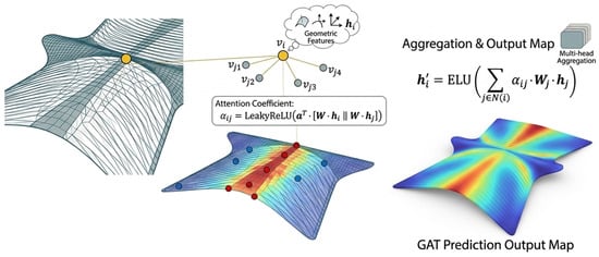
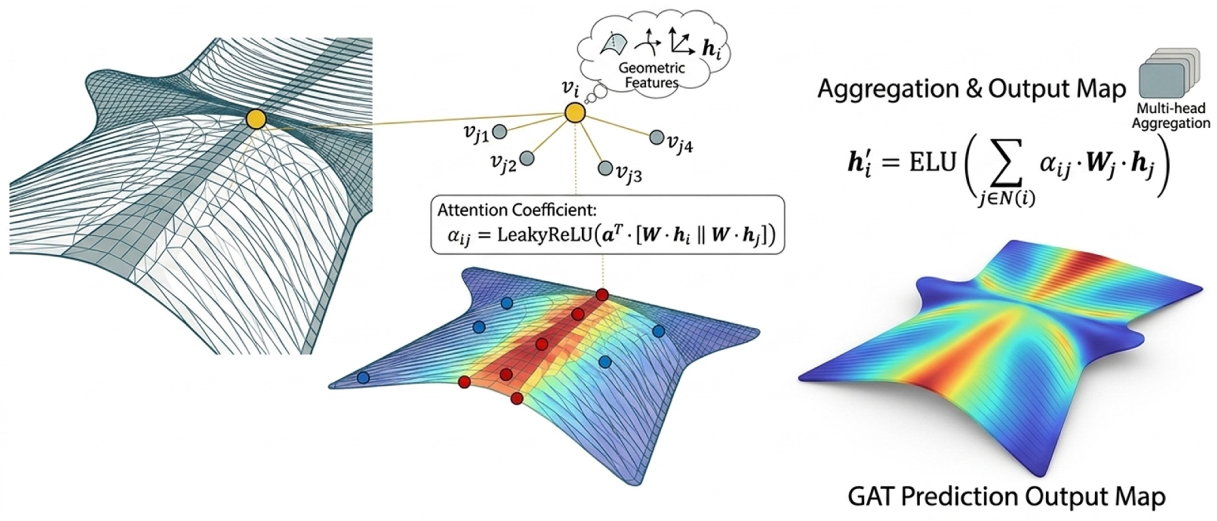
As shown in Figure 1, the GAT model is introduced to characterize the spatial correlations of wind pressure on the curved roof. Each pressure tap is represented as a graph node, and the graph edges encode the neighborhood relationships among taps with spatial proximity and aerodynamic interaction. The node feature vector is first projected into a latent feature space through a shared linear transformation. Then, for each target node, the attention coefficient between the node and its neighbor is computed using a learnable attention function based on the concatenated transformed features, followed by a Leaky ReLU activation, as indicated in the schematic [28,29].
Figure 1.
Schematic of the Graph Attention Network for wind pressure prediction.
Afterward, the attention coefficients are normalized within the neighborhood of each target node to obtain the final weights. These weights are used to perform a weighted summation of the neighboring node features, and the result is passed through a nonlinear activation function to generate the updated embedding [30]. Since the normalization is carried out separately for each node, the attention weights are not necessarily symmetric, which allows the model to adaptively reflect the directional and heterogeneous nature of wind pressure interactions on the roof surface.
To improve feature expressiveness and training robustness, the model adopts a multi-head attention strategy. Several attention heads are executed in parallel to learn diverse local interaction patterns. The feature maps obtained from different heads are concatenated in the hidden layers and averaged in the final prediction layer, as illustrated in Figure 1. This design enables GAT to extract informative spatial features from complex curved roof topologies and enhances its capability to predict wind pressure distributions under limited measurement conditions [31].
The prediction performance of the aforementioned model is evaluated using the following three evaluation indicators: mean absolute error (MAE), root mean square error (RMSE) and coefficient of determination (R2). Their definitions are as follows:
where and yi represent the predicted results and measured data, respectively, is the average value of the measured data, and N represents the total number of measured samples. A value of R2 closer to 1 and RMSE closer to 0 indicate higher prediction accuracy.
3. Hybrid Model Construction
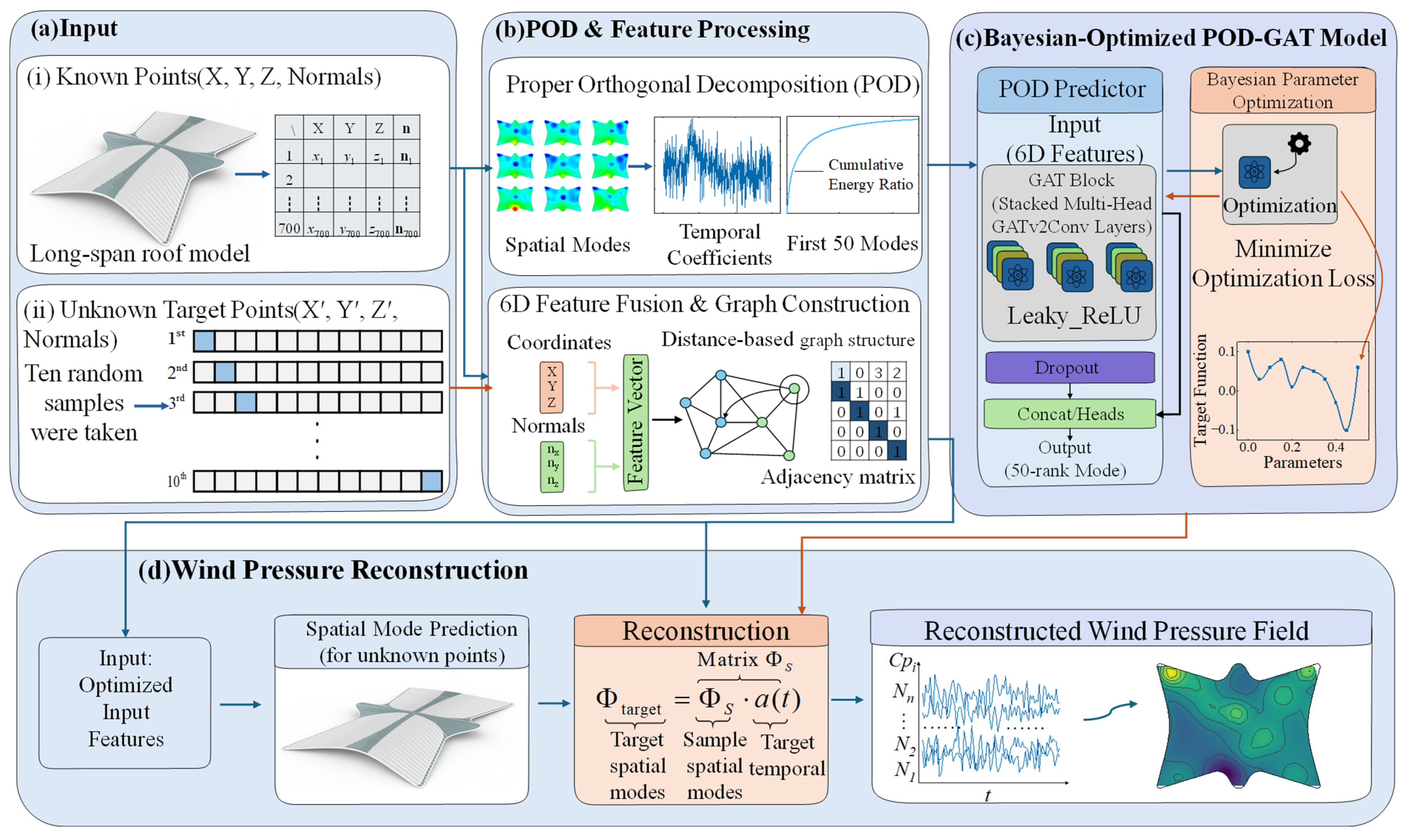
To improve computational efficiency while preserving the dominant characteristics of the fluctuating wind pressure field, Proper Orthogonal Decomposition (POD) is first employed for dimensionality reduction [32]. Specifically, the fluctuating wind pressure field is decomposed into a set of spatial modes and their corresponding temporal coefficients. The energy contribution of each mode is then evaluated based on the singular values. As shown in Figure 2b, based on the fluctuating-pressure data from the complete investigated roof surface covered by the pressure taps, the first 50 POD modes retain 96.7% of the total fluctuating-pressure energy. This energy ratio is calculated as the sum of the first 50 POD eigenvalues divided by the sum of all POD eigenvalues, whereas the contribution of each mode beyond the 50th mode is less than 0.05%. Therefore, only the first 50 modes are retained in this study to balance computational efficiency and reconstruction accuracy.
Figure 2.
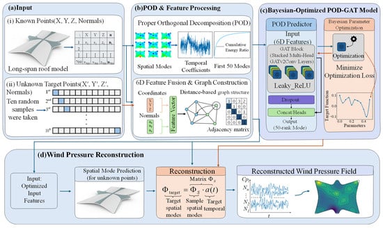
Framework of the Bayesian-optimized POD-GAT model for wind pressure reconstruction and prediction.
After determining the retained POD modes, the geometric input features for the hybrid models are constructed, as illustrated in Figure 2a. The input data consist of two categories of points, namely measured points and unmeasured target points. For each point, a six-dimensional geometric feature vector is defined using its three-dimensional coordinates and the corresponding surface normal components. Ten pressure-tap locations were selected to illustrate the reconstruction performance at representative positions across the investigated roof surface, including regions with different pressure characteristics and locations affected by pronounced flow separation or surface curvature. These locations were chosen for visualization and detailed comparison of reconstructed pressure histories, rather than as a statistical sample for evaluating whole-roof performance. The overall quantitative performance metrics were calculated using all evaluated pressure locations.
The available wind-pressure samples were divided into training and testing sets at a ratio of 7:3. The training set was used to construct the POD basis and train the prediction models, while the testing set was reserved exclusively for independent performance evaluation. To avoid information leakage, the POD basis was constructed only from the training samples and kept fixed during testing. The testing pressure fields were reconstructed using this fixed POD basis, and the model performance was evaluated using the mean absolute error (MAE), root mean square error (RMSE), and coefficient of determination (R2).
Based on the retained POD modes, four POD-based hybrid models are constructed, namely POD-RBF, POD-MLP, POD-CNN, and POD-GAT. In these models, the geometric features of the pressure taps serve as the inputs, while the modal components associated with the retained POD modes at unmeasured locations serve as the prediction targets. The predicted modal components are then used to reconstruct the corresponding wind pressure field.
Among the four models, the RBF, MLP, and CNN models are adopted as benchmark methods. Their basic architectures and training procedures have been extensively reported in previous studies and are therefore not repeated here in detail. In the present study, these models are used to predict the retained POD modal components from the geometric features of the pressure taps. Specifically, the RBF model establishes a nonlinear mapping between the geometric features and the modal components using Gaussian radial basis functions. The MLP model predicts the modal components through a shallow fully connected architecture, whereas the CNN model captures local feature patterns through one-dimensional convolution operations for the same task. The corresponding hyperparameter settings of these benchmark models are summarized in Table 1.
Table 1.
Main hyperparameter settings of the four models.
The proposed POD–GAT model is constructed as follows. First, all wind-pressure measurement points are represented as graph nodes, and each node is characterized by a six-dimensional geometric feature vector consisting of its spatial coordinates and surface-normal components. Subsequently, graph edges are constructed using the K-nearest-neighbor (KNN) algorithm, in accordance with the spatial continuity of the wind-pressure distribution. The number of nearest neighbors, k, is treated as a tunable hyperparameter and is automatically determined through Bayesian optimization based on the validation performance of the GAT model. Within the prescribed hyperparameter search space, the optimal value was found to be k = 15. This graph-construction strategy enables the model to capture local geometric relationships among pressure taps and learn the spatial dependencies between measured and unmeasured locations. As shown in Figure 2b, the resulting graph is represented by a node–feature matrix and an adjacency matrix, which are jointly input into the GAT model.
The four-layer GATv2 architecture was selected to support progressive information aggregation across multiple graph neighborhoods. Four attention heads were used in each of the first three layers to capture complementary spatial relationships, whereas a single head was used in the final layer to produce a unified output. The hidden dimension was set to 16 to balance the representation capacity and model complexity for predicting the reduced-order POD features. Although this compact configuration helps limit the risk of overfitting, such a risk cannot be excluded entirely. Generalization was therefore assessed using the held-out 30% testing set; the POD basis was constructed solely from the training data and fixed during testing. respectively. Specifically, the first three layers employ multi-head attention to learn spatial correlations from different feature subspaces in parallel, and the outputs of the attention heads are concatenated to enhance the representation capability. The final layer uses a single attention head to project the learned node features onto the output space associated with the retained POD modal components, thereby yielding the predicted modal components at the target points. Leaky ReLU is adopted as the activation function, and Dropout is incorporated to alleviate overfitting. The detailed architecture is shown in Figure 2c.
To ensure a fair comparison, all models use the same normalized geometric features as their basic input descriptors. For the GAT model, these node features are additionally combined with graph connectivity information derived from the K-nearest-neighbor (KNN) construction. As shown in Figure 2c, Bayesian optimization is used to determine the hyperparameter configuration of each model. For each candidate configuration, the model is trained and evaluated using the same 10-fold spatial cross-validation procedure, and the mean validation loss across the 10 folds is used as the optimization objective. Thus, the spatial folds are used for hyperparameter selection and model comparison; they do not constitute an independent test set, and the reported cross-validation performance should not be interpreted as an unbiased estimate of performance on an independent spatial test set. The MLP model contains two hidden layers with 32 and 64 neurons, respectively, adopts the ReLU activation function, and uses a learning rate of 4 × 10⁻⁴. The CNN model consists of three convolutional layers with a kernel size of 3, a filter configuration of 32–64–32, ReLU activation, max pooling, and a learning rate of 4 × 10⁻⁴. The GAT model employs a hidden feature dimension of 16, an attention head configuration of 4–4–4–1, the Leaky ReLU activation function, a nearest-neighbor number of 15, and a learning rate of 1 × 10⁻⁵.
During training, the POD spatial modal components at the known measurement points are used as supervision labels, and the model parameters are updated by minimizing the mean squared error (MSE) loss using the Adam optimizer. An early stopping strategy is adopted to mitigate overfitting. It should be noted that only the losses associated with the known nodes are involved in backpropagation, whereas the unknown target nodes receive information from neighboring known nodes through graph-based feature propagation. After the spatial modal components at the unknown locations are predicted, they are combined with the corresponding temporal coefficients to reconstruct the wind pressure time histories and, subsequently, the complete wind pressure field, as illustrated in Figure 2d.
4. Wind Tunnel Test
4.1. Experimental Setup
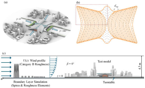
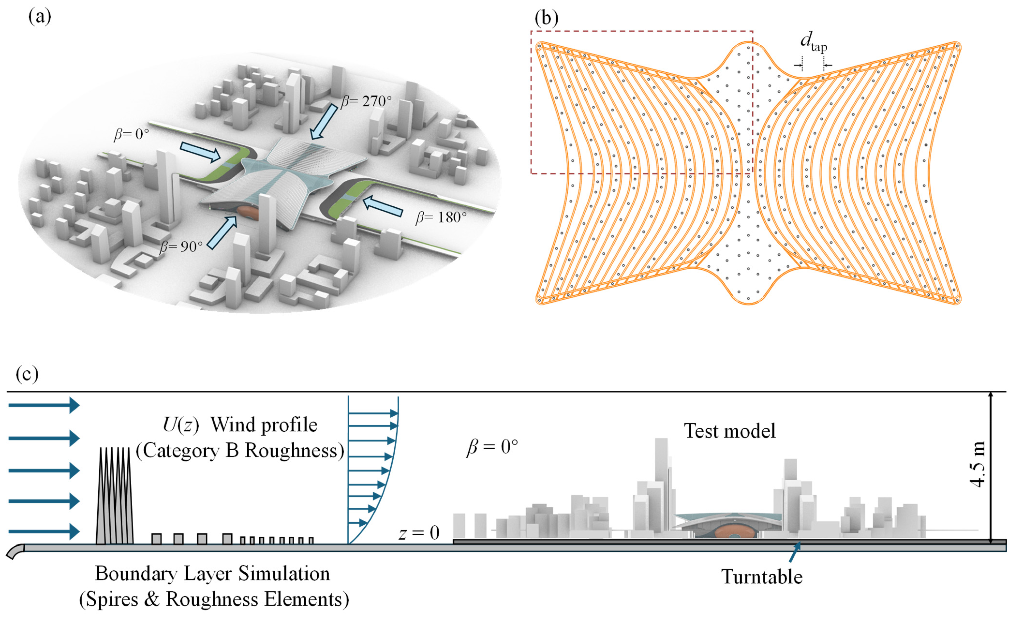
To evaluate the performance of the proposed hybrid model in predicting surface wind pressures on long-span curved roofs, a rigid model wind tunnel test was carried out in the XNJD-3 wind tunnel. The wind tunnel test section is 22.5 m wide, 4.5 m high, and 36 m long, and the available wind speed ranges from 1.0 to 16.5 m/s [33]. The test model represents a long-span high-speed railway station and was constructed from rigid materials, including metal tubes and organic glass, at a geometric scale of 1:200. The resulting blockage ratio is less than 5%, satisfying the relevant test requirements. The model configuration is shown in Figure 3a.
Figure 3.
Experimental setup of the wind tunnel test: (a) wind direction definition; (b) Detail of pressure taps; (c) Wind tunnel test section and inflow boundary layer.
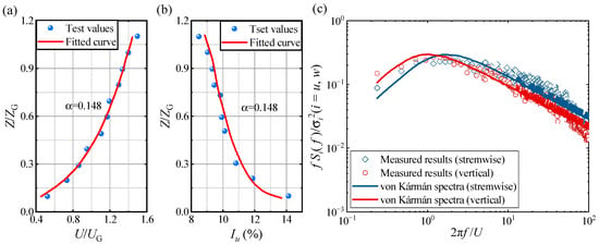
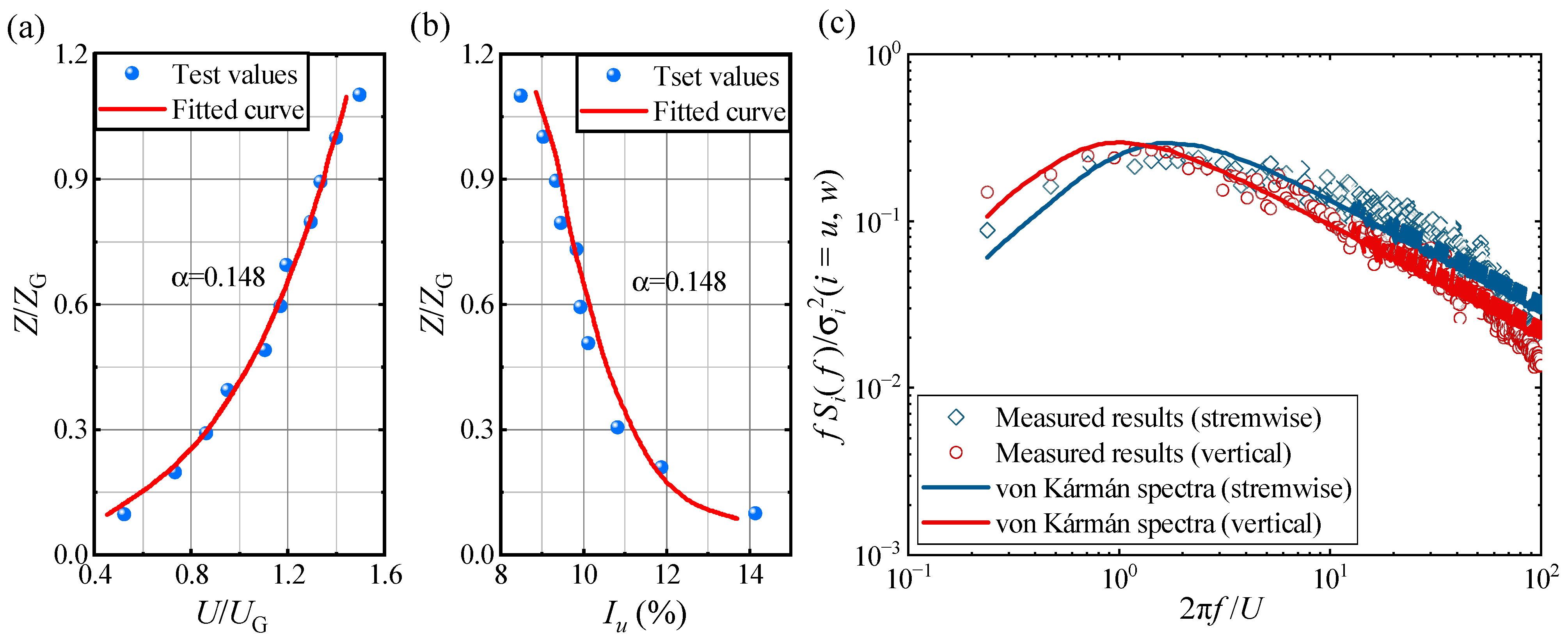
Following GB 50009-2012 [34], the atmospheric boundary layer for Category B terrain was simulated by using spires and roughness elements. The measured wind field characteristics are shown in Figure 4. The mean wind speed profile and turbulence intensity profile agree well with the target profiles, and the measured wind velocity spectra are consistent with the von Kármán spectrum, indicating that the simulated wind field satisfies the required boundary layer characteristics.
Figure 4.
Characteristics of the simulated atmospheric boundary layer: (a) mean wind speed profile; (b) turbulence intensity profile; (c) comparison of measured velocity spectra with the von Kármán spectra in the streamwise and vertical directions.
Surface pressure data were acquired using a Scanivalve DSM4000 pressure measurement system (Scanivalve Corporation, Liberty Lake, WA, USA). The sampling duration was 60 s, and the sampling frequency was 256 Hz, with all pressure taps recorded synchronously. A Cobra Probe (Turbulent Flow Instrumentation Pty Ltd., Tallangatta, VIC, Australia) was also employed to calibrate the incoming flow and to obtain supplementary wind velocity information [35].
A total of 700 pressure taps were arranged over the model surface. Owing to the geometric symmetry of the model about its centerline, the region enclosed by the red boundary in Figure 3b was selected for detailed analysis. To evaluate the within-configuration spatial prediction capability of the proposed model, the pressure taps in the selected region were evenly divided into 10 subsets. Each subset was used in turn as the validation set, while the remaining subsets served as the known measurement points for training. The final predictive performance was evaluated by averaging the error metrics over the 10 runs.
4.2. Data Processing
The wind-pressure records analyzed in this study have a duration of 60 s. This record was used to assess reconstruction performance over the available measurement period; however, the adequacy of a finite record for estimating extreme-pressure statistics depends on the sampling frequency, time-scale conversion, and statistical convergence of the quantities considered. Accordingly, the present results do not establish convergence of long-duration or rare-event extreme-value estimates. Further validation using longer records, repeated realizations, or record-length sensitivity analysis is needed to assess the robustness of extreme-pressure statistics.
The wind pressure time histories measured at each pressure tap in the wind tunnel test were converted into dimensionless wind pressure coefficients.
where Cpi(tj) is the wind pressure coefficient of the ith measuring point of the model, U0 is the mean wind speed at the maximum roof height measured in the undisturbed upstream flow, P∞ is the reference static pressure at this height, Pi(tj) is the pressure at each pressure measuring point of the model, and ρ is the air density. Cp,mean and Cp,rms are the mean pressure coefficient and fluctuating pressure coefficient, respectively, and N represents the total number of pressure measurement points within the measurement point area [36].
On the basis of the mean and fluctuating pressure coefficients, the higher-order statistical moments were further introduced to quantify the non-Gaussian characteristics of the wind pressure signals. In this study, the skewness coefficient and kurtosis coefficient were employed to describe the asymmetry and peak–tail features of the pressure coefficient distribution, respectively, and can be calculated by
Furthermore, to evaluate the ability of the reconstructed wind pressure time histories to reproduce the extreme fluctuations of the original signals, the peak factor was adopted as an additional statistical indicator. Since the local wind pressure on large-span curved roofs may exhibit distinct positive and negative extremes, the peak factor was separately defined for the positive and negative pressure excursions as
where g+ and g− are the positive and negative peak factors, respectively; Cp,max and Cp,min are the maximum and minimum instantaneous wind pressure coefficients during the sampling period; is the standard deviation of the fluctuating pressure coefficient. As a normalized measure of the deviation of extreme pressure from the mean level, the peak factor can effectively reflect the preservation of extreme-value characteristics in the reconstructed wind pressure signals.
5. Prediction Results and Performance Evaluation
Based on the wind tunnel data and the cross-validation scheme described in Section 4, the predictive performance of the proposed models is evaluated in terms of modal prediction accuracy, reconstruction of wind pressure coefficients, time-history agreement, and spectral consistency.
5.1. Modal Prediction
The fluctuating wind pressure field on long-span roofs is highly complex owing to the combined effects of incoming turbulence and the aerodynamic characteristics of the roof geometry. According to the POD energy accumulation analysis, the first 50 POD modes retain 96.7% of the fluctuating wind pressure energy and thus capture the dominant characteristics of the pressure field. Therefore, accurate prediction of these dominant modal components is essential for the subsequent reconstruction of wind pressure time histories and the complete pressure field at unmeasured locations. To evaluate the feasibility and predictive capability of the proposed POD-based hybrid models, this section compares the performance of the four models in predicting the dominant POD modes of the fluctuating wind pressure field.
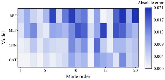
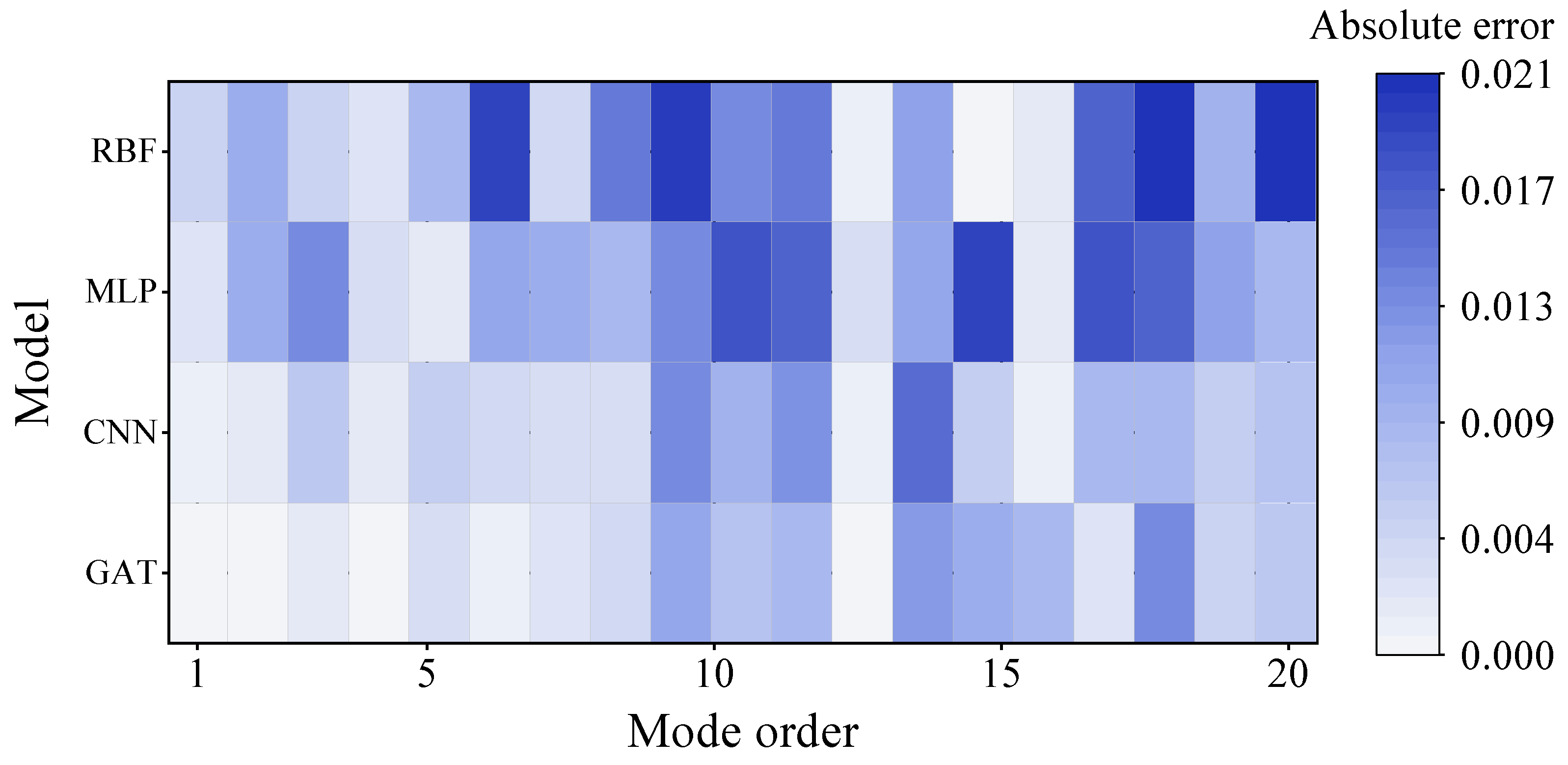
To further compare the modal prediction performance of the four hybrid models, Figure 5 presents the absolute prediction errors for the first 20 dominant POD modes. The corresponding numerical values are provided in Appendix A (Table A1). Since 50 modes were retained for pressure reconstruction, the results shown here characterize only a subset of the retained modal subspace and should not be interpreted as a comprehensive assessment of all retained modes. Overall, the modal components predicted by all four models agree reasonably well with the corresponding reference values, indicating that each model is able to capture the principal characteristics and variation trends of the dominant modes to a certain extent. Nevertheless, noticeable differences in prediction accuracy can still be observed among the models. In particular, the GAT and CNN models exhibit superior performance in modal prediction. For most of the first 20 modes, the prediction errors of these two models remain lower than those of the MLP and RBF models. Among the four models, the GAT model achieves the smallest absolute errors overall, with most values remaining below 0.01, demonstrating its clear advantage in predicting the dominant modal components.
Figure 5.
Comparison of absolute errors of different models across POD mode orders.
For all four models, the prediction error of the POD modes generally increases rapidly at low modal orders and then gradually approaches a relatively stable level as the modal order increases. Nevertheless, both the error magnitude and the stabilization level differ significantly among the models. In the low-order modal range, the errors of the GAT, MLP, and RBF models rise rapidly from values close to zero, whereas the CNN model shows a more gradual increase. Once the modal order exceeds approximately 5, the error curves of the four models tend to enter a relatively stable stage, with noticeably reduced fluctuation amplitudes.
Among the four models, the RBF model consistently exhibits the highest error level across the entire modal range, indicating the weakest capability in predicting the POD modes. The MLP model performs slightly better than the RBF model; however, its overall trend remains similar, and noticeable local error peaks can still be observed in the intermediate modal range, suggesting limited robustness in capturing intermediate-order modal features. By contrast, the CNN model demonstrates better predictive performance, particularly in the low-order modal range, where the increase in error is relatively moderate. After the error curves become stable, its overall error level remains lower than those of the RBF and MLP models. Among all four models, the GAT model delivers the best performance. It not only exhibits the smallest increase in error at the low-order modal stage but also maintains the lowest and most stable error level in the higher-order modal range. These results highlight the effectiveness of the graph attention mechanism in learning the spatial correlation characteristics embedded in the POD modes.
The inferior performance of the conventional models, particularly the MLP and RBF models, can be mainly attributed to their limited ability to represent the complex spatial topology of curved roofs. These models primarily rely on direct feature mapping and are less effective in explicitly characterizing the correlation structure among spatially distributed pressure taps. As a result, their prediction errors tend to become more pronounced in regions with strong geometric variation or severe flow separation, where the spatial distribution of wind pressure is highly complex. In such areas, the underlying pressure patterns cannot be sufficiently captured by the MLP or RBF models. By contrast, the GAT model establishes relationships among pressure taps through graph connectivity and adaptively assigns different weights to neighboring nodes via the attention mechanism. This enables the model to more effectively learn the spatial dependence of the pressure field, thereby achieving higher accuracy in predicting the dominant modal components.
To quantitatively evaluate the predictive performance of the four models, Table 2 summarizes the evaluation metrics at several representative pressure taps under a wind direction of 0°. Combined with the comparison shown in Figure 5, it can be observed that all four models achieve coefficients of determination R2 greater than 0.80, indicating that each model is capable of capturing the general variation trend of the target responses. However, the GAT model consistently provides the best prediction performance, followed by the CNN, MLP, and RBF models. At all selected taps, the GAT model yields the lowest MAE and RMSE values as well as the highest R2 values. Specifically, the R2 values of the GAT model reach 0.9397 at A2, 0.9235 at B6, 0.9256 at E5, and 0.9052 at S13, all of which are higher than those of the other three models. These results further demonstrate that the GAT model can more accurately predict the wind pressure responses at unmeasured locations.
Table 2.
Model evaluation metrics.
In addition, at locations such as A2 and S13, where flow separation is relatively significant and geometric effects are more pronounced, the superiority of the GAT model becomes even more evident. Compared with the MLP and RBF models, GAT significantly reduces the prediction error, and it also outperforms CNN by a noticeable margin. This indicates that the proposed POD-GAT method is capable of effectively capturing the spatial dependence between pressure taps at different locations. Consequently, it achieves robust and accurate predictions even in regions with severe flow separation and substantial curvature variation on long-span curved roofs.
5.2. Modal Sensitivity Analysis
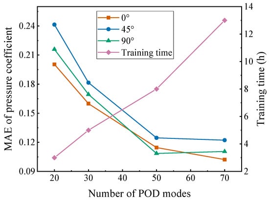
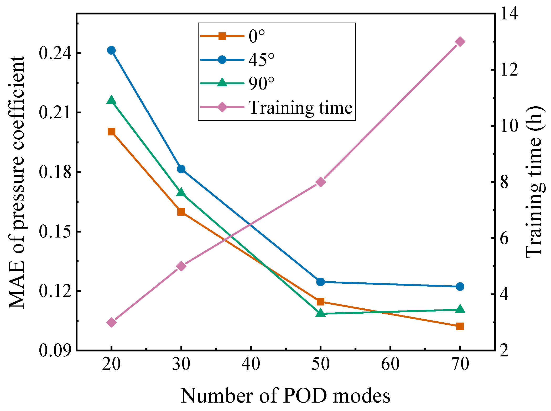
To investigate the sensitivity of the pressure reconstruction performance to the POD truncation order, additional analyses were conducted using r = 20, 30, 50, and 70 retained modes. For each truncation level, the POD basis was reconstructed independently, and the corresponding GAT model was retrained using the same training, validation, and testing subsets. The network architecture, optimization strategy, and training conditions were kept unchanged to ensure a consistent comparison.
As shown in Figure 6, increasing the number of retained modes from 20 to 50 substantially reduces the MAE for all three wind directions. Specifically, the MAE decreases from approximately 0.20, 0.24, and 0.22 to 0.115, 0.124, and 0.109 for 0°, 45°, and 90°, respectively. Further increasing the truncation order to 70 provides diminishing benefits: the MAE decreases further for 0°, remains nearly unchanged for 45°, and increases slightly for 90°. Meanwhile, the training time increases from approximately 3 h at r = 20 to 8 h at r = 50 and 13 h at r = 70.
Figure 6.
Effect of the Number of Retained POD Modes on Wind Pressure Reconstruction Accuracy and Training Time.
These results indicate that retaining 50 modes provides a reasonable balance between reconstruction accuracy and computational cost. This choice is also consistent with the POD energy analysis, as the leading 50 modes capture 96.7% of the fluctuating-pressure energy. Therefore, r = 50 was adopted in this study.
5.3. Wind Field Reconstruction
To further evaluate the predictive performance of the proposed POD-GAT model, the original wind pressure time-history signals at unmeasured locations are reconstructed by combining the spatial modes predicted in Section 5.1 with the corresponding POD temporal coefficients. Because the fluctuating wind pressure field is represented in POD as the superposition of spatial modes and time-dependent modal coefficients, the reconstruction accuracy of the wind pressure time histories provides a direct measure of the effectiveness of the proposed method.
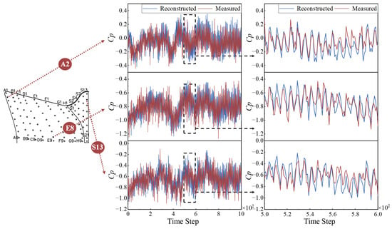
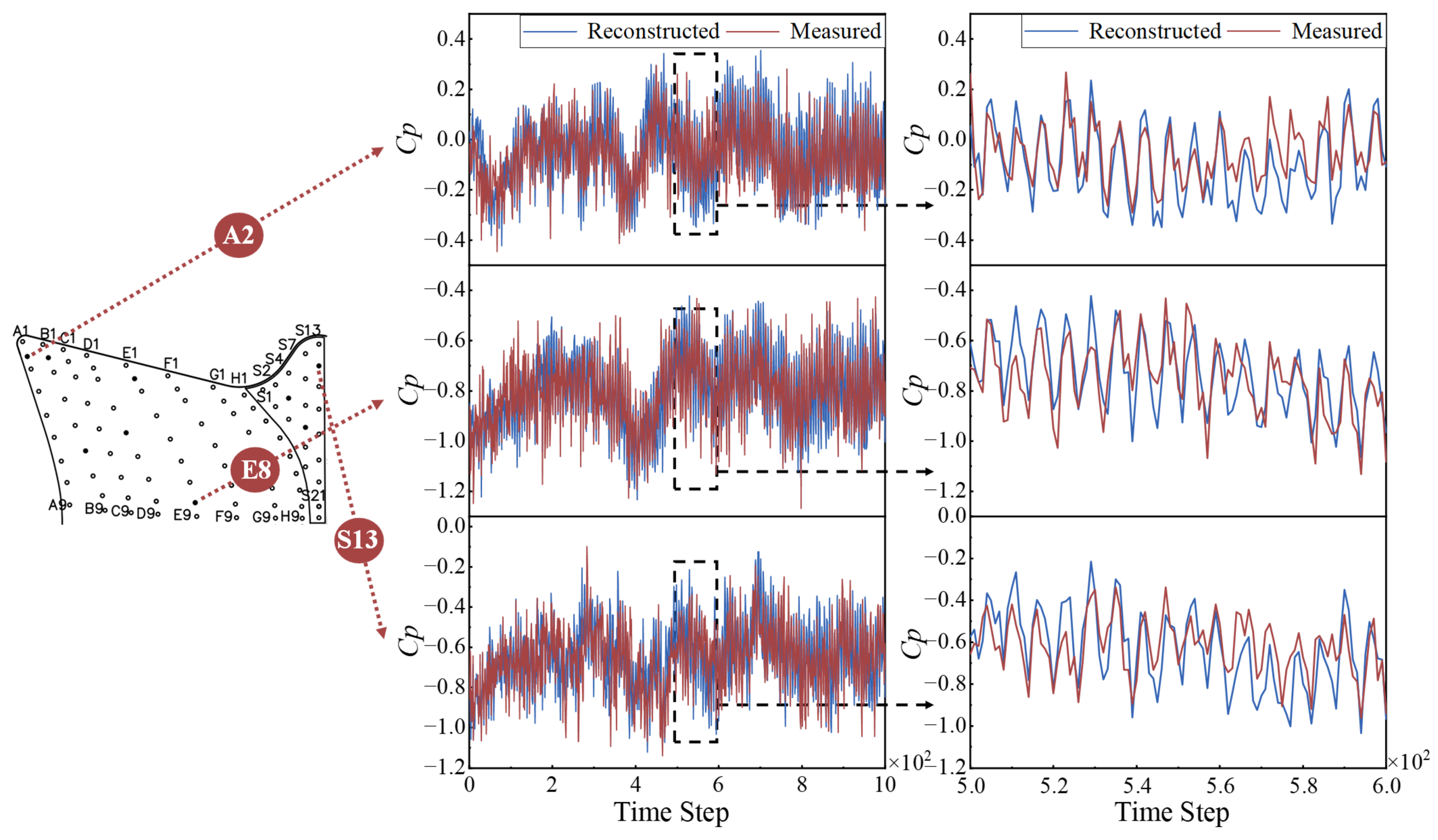
Representative pressure taps A2, E8, and S13 are selected as typical examples for validation. As shown in Figure 7, the reconstructed wind pressure coefficient time histories agree well with the measured results at all selected locations. The POD-GAT predictions accurately reproduce the overall variation trend and major fluctuation characteristics of the measured signals. In addition, the local enlarged views show that the predicted extrema are located very close to the measured values, without obvious phase shift or systematic amplitude deviation. To quantitatively assess the agreement shown in Figure 6, the MAE and RMSE between the reconstructed and measured pressure-coefficient time histories were calculated for taps A2, E8, and S13. The RMSE values were 0.0439, 0.0846, and 0.1032, respectively, while the corresponding MAE values were 0.0327, 0.0627, and 0.0972. This indicates that the proposed method can effectively capture both the global temporal evolution and the local transient features of wind pressure fluctuations.
Figure 7.
Time-history comparison of reconstructed and measured wind pressure coefficients at representative pressure taps.
The above results demonstrate that the POD-GAT model is capable of accurately reconstructing wind pressure time histories at unmeasured points on long-span curved roofs. Combined with the results of modal prediction in Section 5.1, this further confirms that the proposed framework can not only predict the dominant POD spatial modes with high accuracy but also provide reliable reconstruction of the original unsteady wind pressure field. Such a capability is of practical significance for wind-resistant design and local pressure assessment of complex long-span roof structures.
5.4. Mean and Fluctuating Pressure Coefficients
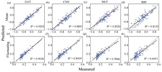
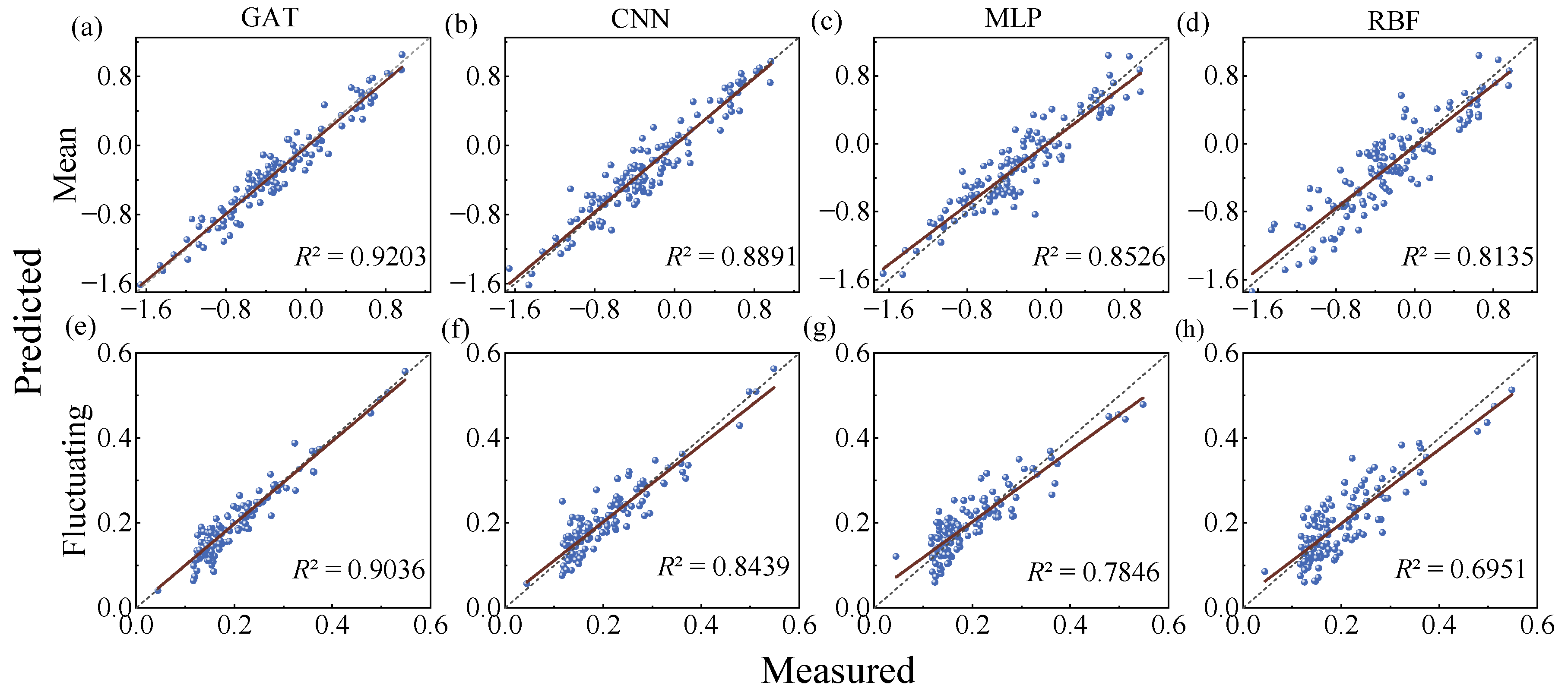
To avoid bias caused by spatially uneven generalization, all pressure taps in the study region were evenly divided into 10 subsets. In each round, one subset was treated as unmeasured points for validation, and the remaining subsets were used for training. This process was repeated 10 times, and the average results were used to evaluate model performance. Figure 8 shows the predicted versus measured mean and fluctuating wind pressure coefficients obtained by the four models, respectively, with R2 and MAE used as evaluation metrics.
Figure 8.
Comparison of predicted versus measured mean and fluctuating wind pressure coefficients for different models: (a) GAT for mean values; (b) CNN for mean values; (c) MLP for mean values; (d) RBF for mean values; (e) GAT for fluctuating values; (f) CNN for fluctuating values; (g) MLP for fluctuating values; and (h) RBF for fluctuating values. Blue dots represent the predicted–measured data pairs, the gray dotted lines indicate perfect agreement (y = x), and the brown solid lines represent the linear regression fits.
The results indicate that all models can generally capture the variation trend of the wind pressure coefficients, but their prediction accuracies differ significantly. For both mean and fluctuating wind pressure coefficients, GAT yields the best overall performance, followed by CNN, MLP, and RBF. Specifically, for the mean wind pressure coefficient, the R2 values of GAT, CNN, MLP, and RBF are 0.9203, 0.8891, 0.8526, and 0.8135, respectively. For the fluctuating wind pressure coefficient, the corresponding R2 values are 0.9036, 0.8439, 0.7846, and 0.6951. The scatter points predicted by GAT are distributed most closely around the diagonal line, indicating the highest consistency with the measured results.
The superior performance of GAT can be attributed to its ability to model spatial topological relationships among pressure taps and to adaptively aggregate neighborhood information through the attention mechanism. This enables the model to better capture complex local aerodynamic effects, such as flow separation and vortex-induced fluctuations, especially in regions with strong suction or large pressure fluctuations. By contrast, MLP and RBF do not explicitly account for spatial correlations and therefore show larger prediction deviations in complex flow regions. Although CNN benefits from local feature extraction, it still lacks the flexibility to represent irregular inter-point dependencies on complex curved surfaces. These results confirm the effectiveness of the proposed graph-based framework for wind pressure prediction on long-span curved roofs.
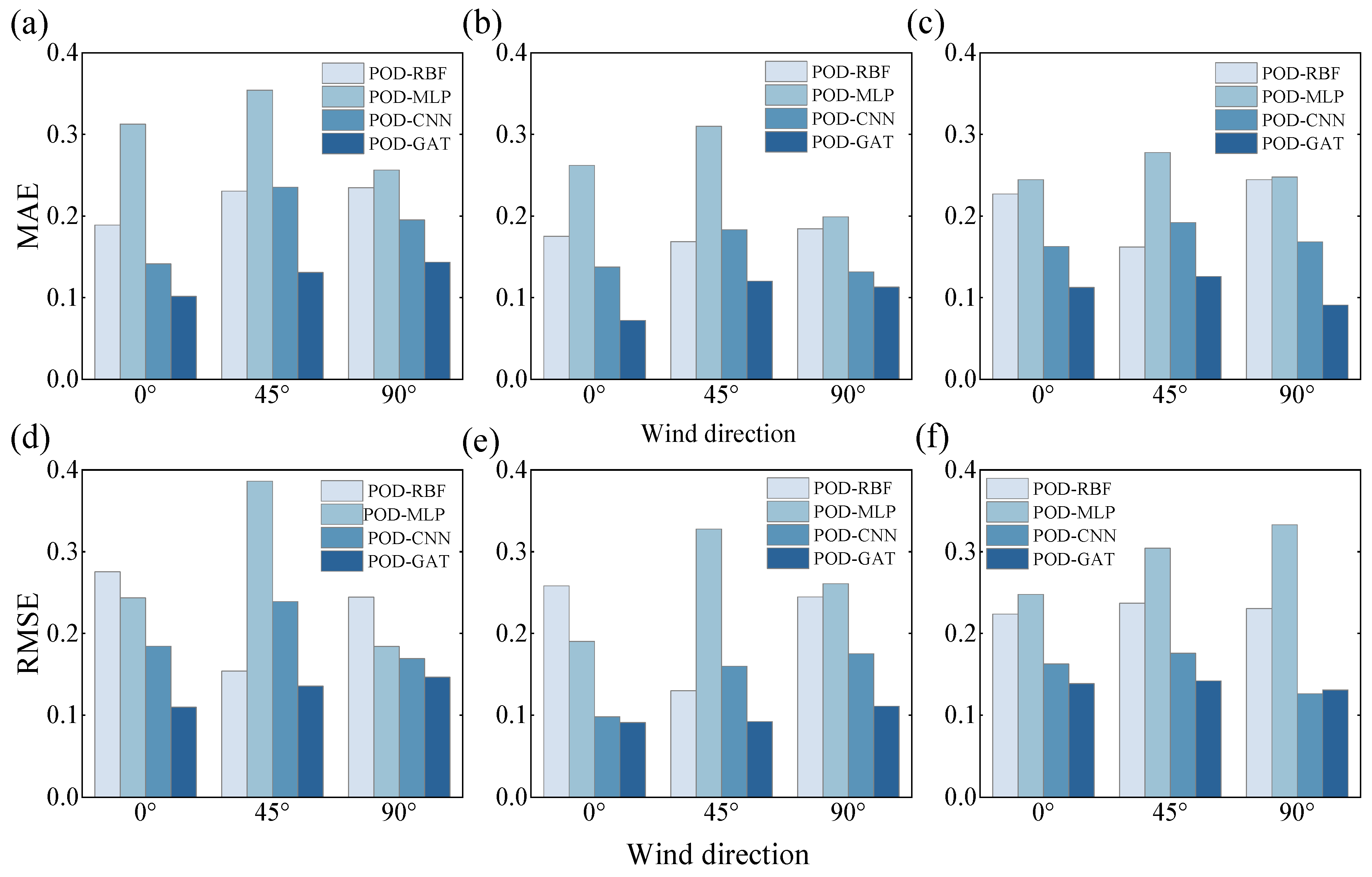
To evaluate the prediction performance of POD-GAT under different wind directions, Figure 9 compares the MAE and RMSE of the mean and fluctuating wind pressure coefficients predicted by different hybrid models at representative pressure taps A2, E8, and S13 under 0°, 45°, and 90° wind directions. Overall, all hybrid models show acceptable prediction performance, with both MAE and RMSE remaining below 0.30 even though the target taps are not involved in training. Among them, POD-GAT achieves the smallest errors, generally around 0.10. Thus, the results demonstrate robustness across the tested wind directions within the present configuration, rather than generalization to arbitrary aerodynamic conditions.
Figure 9.
Comparison of the MAE and RMSE of different POD-based models under various wind directions: (a) A2 for MAE; (b) E8 for MAE; (c) S13 for MAE; (d) A2 for RMSE; (e) E8 for RMSE; (f) S13 for RMSE.
The prediction accuracy varies with both wind direction and tap location. Larger errors occur at taps such as A2 and S13, where the roof curvature changes abruptly, or flow separation is more severe. In addition, the model performance is influenced by wind direction because different incoming flow angles alter the separation, reattachment, and non-Gaussian characteristics of the roof flow field. In particular, under the 45° wind direction, the RMSE of POD-GAT reaches a maximum of about 0.15, suggesting that the conical vortices formed under oblique wind incidence increase the complexity of local aerodynamic behavior. Therefore, in practical applications, additional pressure taps should be arranged in edge regions or areas with large pressure variations to further improve the prediction accuracy of the POD-GAT model.
5.5. Power Spectral Density
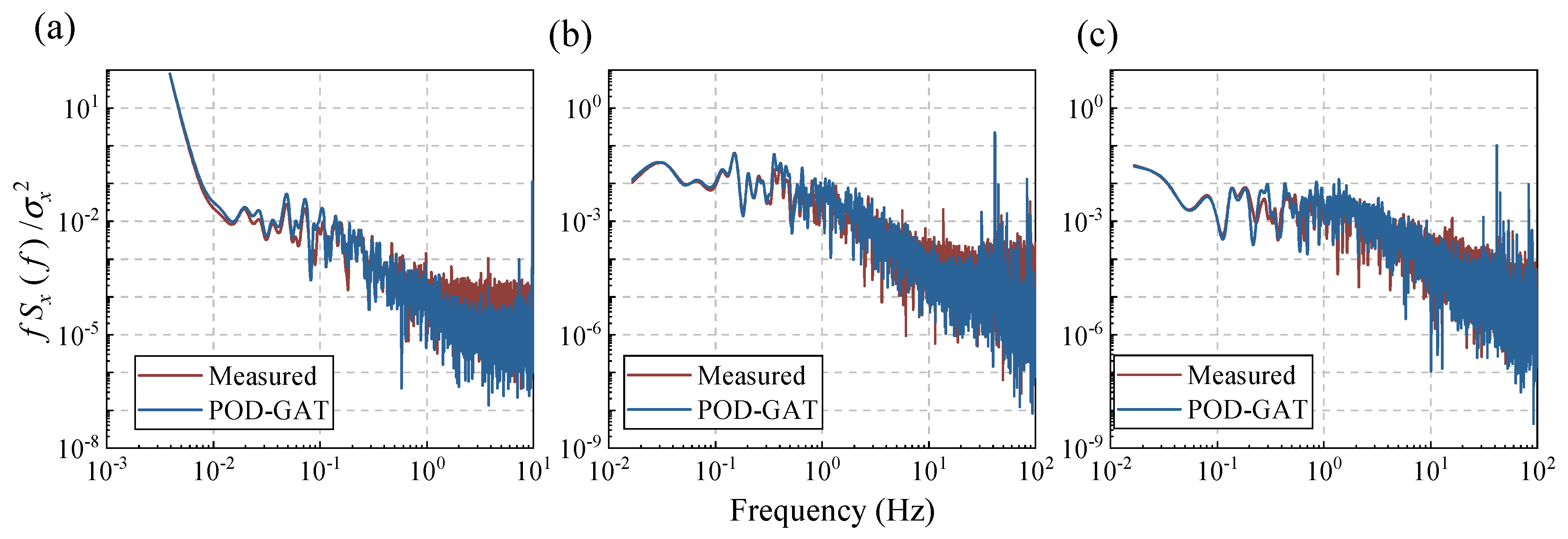
In addition, the frequency-domain prediction performance of the POD-GAT model is further evaluated in Figure 10, which compares the power spectral density (PSD) of the predicted and measured wind pressure signals at pressure tap E8 under wind direction angles of 0°, 45°, and 90°. Although the target pressure tap is excluded from the training set, the predicted spectra show good agreement with the wind tunnel test results over most of the frequency range. In particular, the POD-GAT model is able to reproduce the dominant spectral characteristics and the overall energy distribution of the wind pressure fluctuations under different wind directions.
Figure 10.
Comparison of power spectral densities between wind tunnel tests and POD-GAT predictions at the same pressure tap under different wind directions: (a) 0°; (b) 45°; (c) 90°.
It can also be observed that a certain loss of high-frequency energy appears in the predicted spectrum, especially in the frequency range above 10 Hz. This phenomenon is directly related to the POD truncation process adopted in the present study. Since POD reconstruction retains only the first 50 dominant modes, some higher-order modal information associated with small-scale and high-frequency fluctuations is inevitably discarded. However, according to the POD energy accumulation results, the first 50 modes already account for 96.7% of the total energy of the wind pressure field, while the contribution of the remaining higher-order modes is less than 4%. Accordingly, although the reconstructed pressure spectra exhibit a loss of energy above approximately 10 Hz, the implications of this loss for engineering quantities—such as local peak pressures, extreme suctions, and fatigue-related responses—have not been quantified in this study and warrant further investigation.
Overall, the results indicate that the POD-GAT model can not only accurately reconstruct the time-domain variation in wind pressure signals but also preserve their principal frequency-domain characteristics. Similar prediction performance is observed at other unmeasured pressure taps, further demonstrating the robustness and within-configuration spatial prediction capability of the proposed method in wind pressure field reconstruction.
5.6. Non-Gaussian Characteristics
To further assess whether the proposed POD-GAT model can preserve the non-Gaussian statistical characteristics of wind pressure fluctuations, the reconstructed pressure time histories were examined from four aspects: the probability density function (PDF), cumulative distribution function (CDF), skewness–kurtosis relationship, and peak factor.
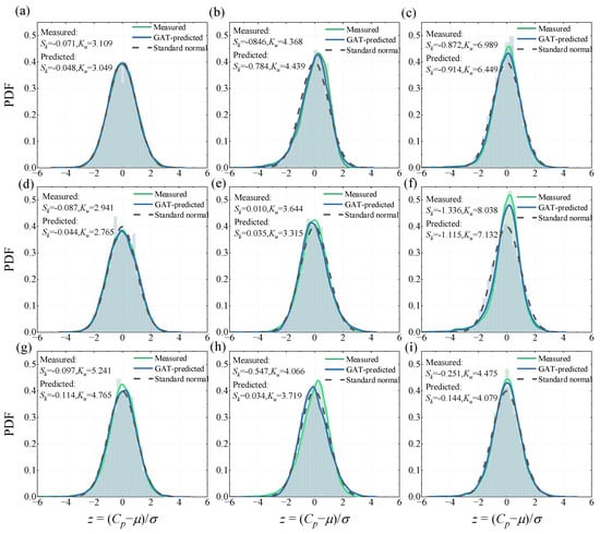
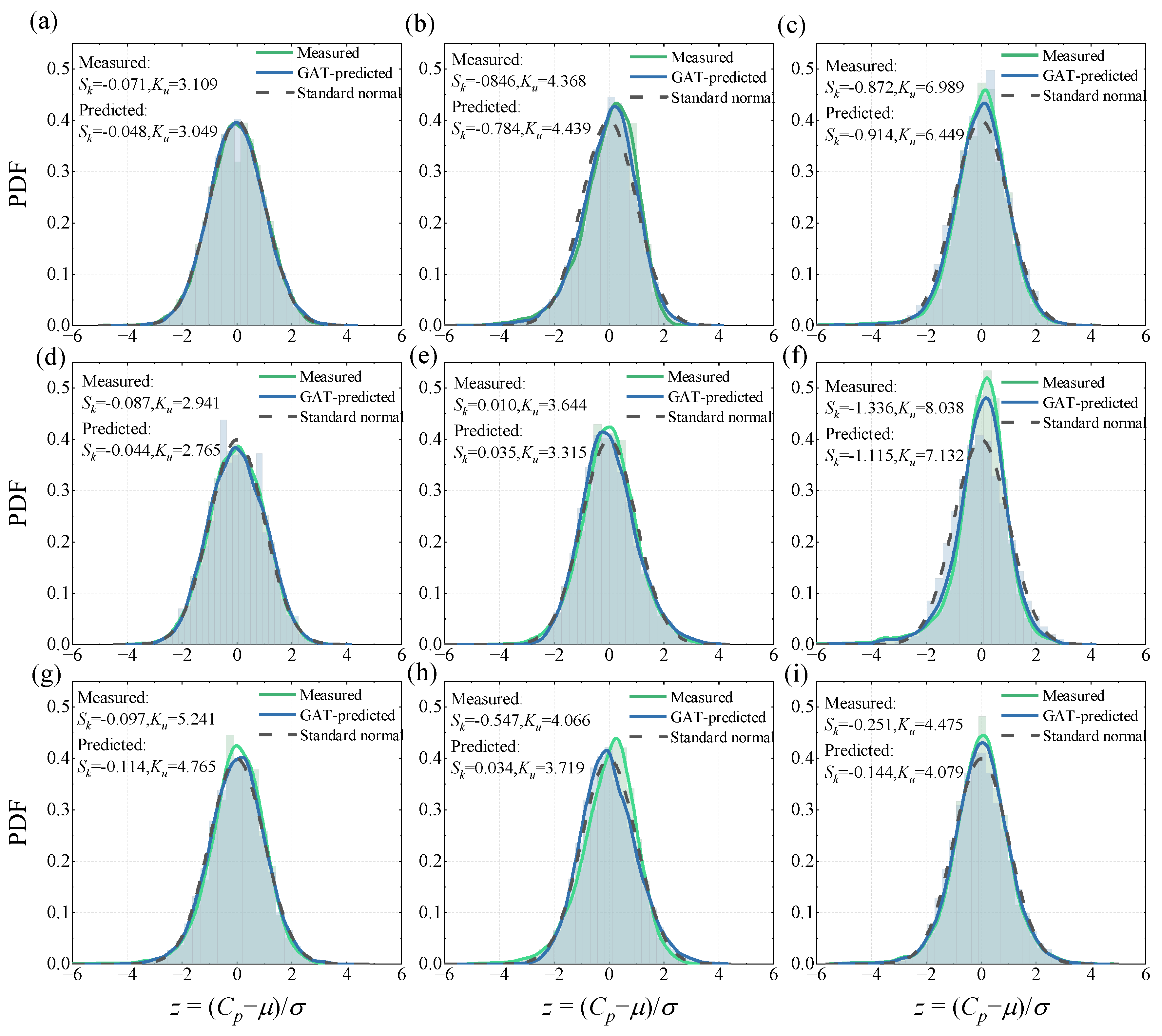
Figure 11 compares the PDFs of the standardized pressure coefficient at several representative pressure taps under different wind directions, together with the standard normal distribution as a reference. In general, the measured wind pressure signals deviate appreciably from the Gaussian distribution, indicating pronounced non-Gaussian characteristics in local pressure fluctuations over the long-span curved roof. These deviations are mainly manifested in distribution asymmetry and enhanced tail probabilities, particularly in regions associated with strong suction and flow separation.
Figure 11.
Comparison of measured and predicted probability density functions of the standardized pressure coefficient at representative taps: (a) A2, 0°; (b) E8, 0°; (c) S13, 0°; (d) A2, 45°; (e) E8, 45°; (f) S13, 45°; (g) A2, 90°; (h) E8, 90°; (i) S13, 90°.
For relatively weakly non-Gaussian cases, the predicted and measured PDFs are both close to the standard normal distribution. This indicates that the POD-GAT model can accurately reproduce pressure signals whose skewness is close to 0 and kurtosis is close to 3. By contrast, for strongly non-Gaussian cases, the measured distributions exhibit evident left-skewness and leptokurtic behavior. For example, at tap S13 under a wind direction of 0°, the measured skewness and kurtosis are −0.872 and 6.989, respectively, while the corresponding predicted values are −0.914 and 6.449. The close agreement between these values indicates that the POD-GAT model is able to preserve both the negative skewness and the heavy-tailed nature of the measured signal. A similar pattern is observed for another strongly non-Gaussian case, where the measured skewness and kurtosis are −1.336 and 8.038, compared with predicted values of −1.115 and 7.132. Although the tail intensity is slightly underestimated, the reconstructed signal still retains the essential left-skewed and leptokurtic features.
Overall, the predicted PDFs agree well with the measured distributions in terms of peak location, overall shape, and the sign and magnitude of non-Gaussianity. Some discrepancies remain in the tails under strongly non-Gaussian conditions, but the proposed model still captures the principal distributional characteristics of the original wind pressure signals. This provides a sound basis for the subsequent evaluation of CDFs, higher-order statistical moments, and peak factors.
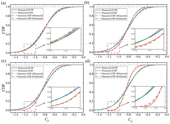
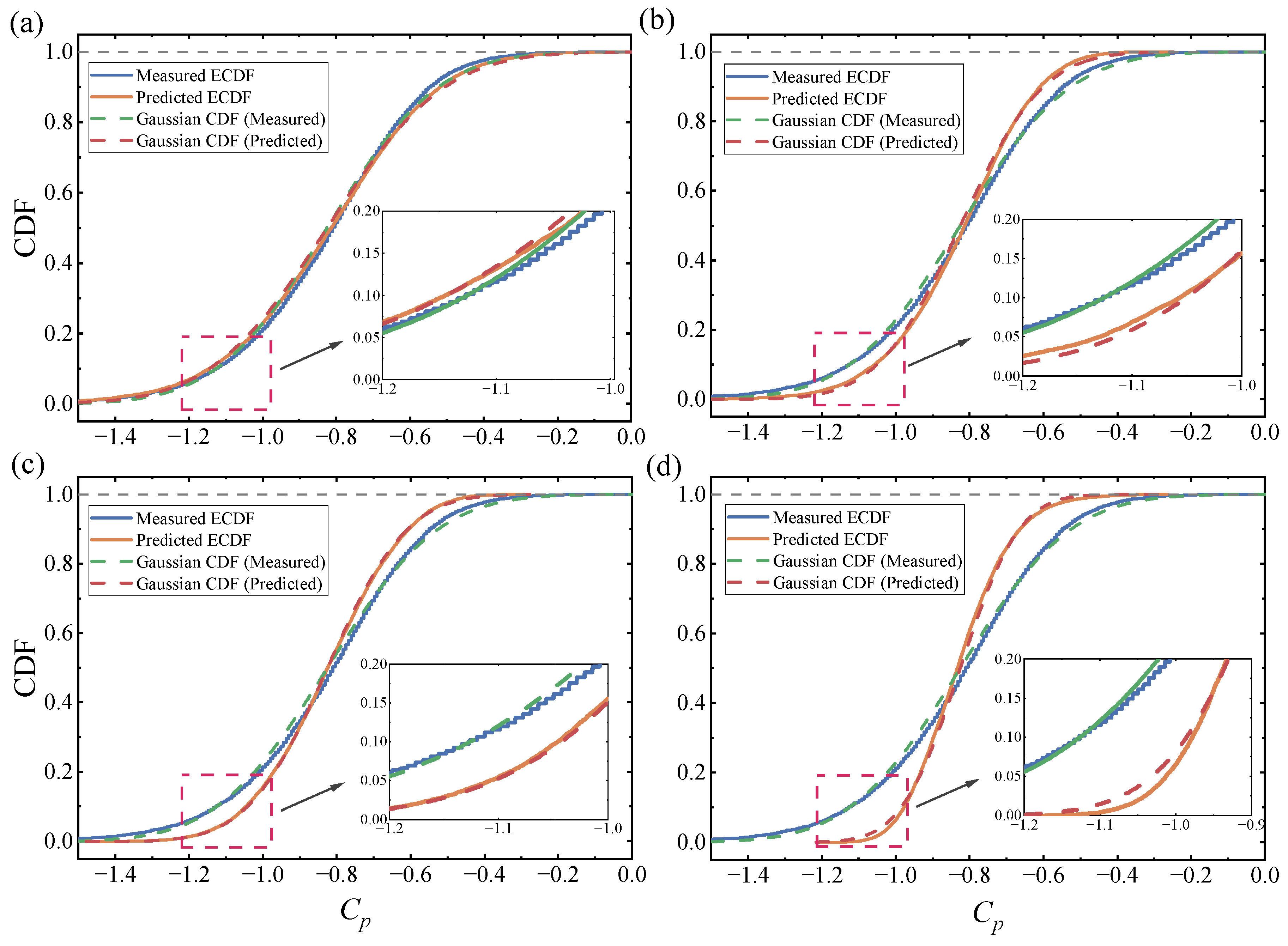
While the PDF comparison in Figure 11 reflects the overall distribution shape of the reconstructed signals, the cumulative distribution function provides a more sensitive measure of tail-related probabilistic behavior. Therefore, Figure 12 further compares the empirical cumulative distribution functions (ECDFs) of the measured and reconstructed pressure signals at tap S13 for different POD-based models, together with their corresponding Gaussian reference CDFs.
Figure 12.
Comparison of measured and predicted cumulative distribution functions at tap S13 for four models: (a) POD-GAT; (b) POD-CNN; (c) POD-MLP; (d) POD-RBF.
As shown in Figure 12, the measured ECDF departs markedly from the Gaussian reference, particularly in the negative tail region, indicating pronounced non-Gaussian characteristics at this tap. This behavior is physically plausible because S13 is located in a region of strong local suction, where the pressure response is strongly affected by intermittent flow structures associated with flow separation, shear-layer instability, and vortex-induced suction events. Under such conditions, the pressure signal tends to contain sporadic large-amplitude negative peaks, leading to an enhanced lower tail that cannot be adequately represented by a Gaussian assumption.
Among the four models, the POD-GAT prediction shows the closest agreement with the measured ECDF across most of the probability range, with the advantage being especially evident in the enlarged negative-tail region. This suggests that the proposed model captures not only the main body of the distribution, but also the tail-related probabilistic characteristics associated with low-probability suction events. In wind engineering, accurate representation of the negative tail is particularly important because it is directly related to the occurrence probability of extreme local suctions that may govern cladding demand and component design.
By contrast, the larger tail discrepancies observed for POD-CNN, POD-MLP, and POD-RBF indicate a weaker capability to reproduce low-probability extreme fluctuations, even when the overall distribution trend is approximately captured. It should be noted that, in the tail region of the CDF, even a small deviation in the curve may correspond to a non-negligible error in the estimated probability of extreme suction occurrence. Consequently, the superior tail fitting of POD-GAT is not merely a statistical improvement; rather, it indicates a better preservation of the non-Gaussian probabilistic characteristics of the original pressure process. This is particularly meaningful for strongly non-Gaussian taps such as S13, where localized flow separation and unsteady vortex action dominate the pressure response.
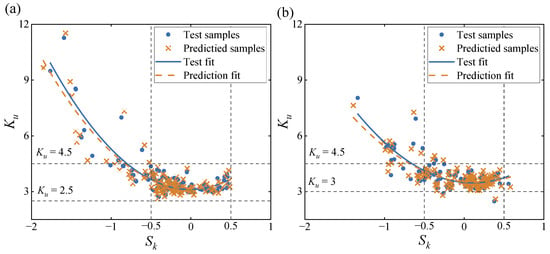
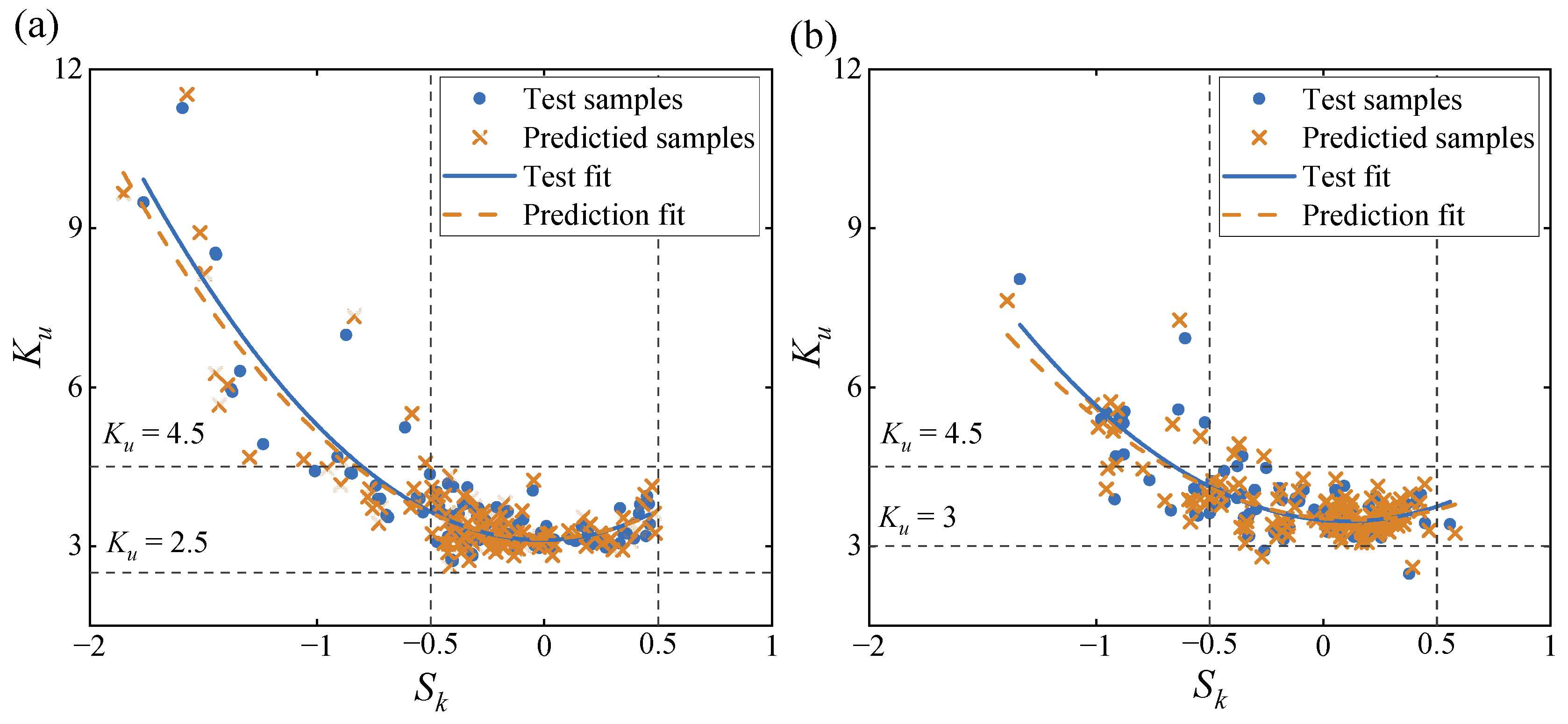
Figure 13 further provides a global view of the higher-order statistical characteristics of the roof pressure field by comparing the skewness–kurtosis distributions of the measured and predicted pressure signals at all taps under different wind directions. The blue circles and orange crosses represent the measured and predicted samples, respectively, while the corresponding fitted curves indicate their overall trends in the skewness–kurtosis plane.
Figure 13.
Comparison of measured and predicted skewness–kurtosis distributions for all pressure taps under different wind directions: (a) 0°; (b) 45°.
It can be seen that most measured samples are concentrated in the region of negative skewness and kurtosis greater than 3, indicating that the roof pressure signals are generally characterized by negatively skewed and leptokurtic distributions relative to the Gaussian reference. This reflects the widespread presence of intermittent suction events and further confirms the non-Gaussian nature of the roof pressure field.
Moreover, the fitted trend reveals an evident correlation between kurtosis and skewness. As the skewness becomes more negative, the kurtosis generally increases, suggesting that signals with stronger asymmetry also tend to exhibit heavier tails and stronger intermittency. This trend is physically consistent with the pressure response in separation-dominated roof regions, where localized vortex action and intermittent suction peaks can simultaneously produce larger negative skewness and higher kurtosis. Therefore, the skewness–kurtosis relationship not only summarizes the global higher-order statistical characteristics of the roof pressure field, but also indicates that locations with stronger negative asymmetry are more likely to be associated with stronger extreme suction.
More importantly, the predicted samples generally follow the distribution pattern of the measured samples, and the fitted prediction curve agrees well with the measured trend over the main concentration region. Although some discrepancies remain in the range of strongly negative skewness and high kurtosis, the POD-GAT model still captures the principal organization of the measured data in the skewness–kurtosis plane. This demonstrates that the proposed method can preserve not only the lower-order statistics of wind pressure signals, but also their global non-Gaussian statistical structure.
Table 3 compares the measured and predicted positive and negative peak factors at representative taps under different wind directions. Overall, the predicted peak factors show reasonable agreement with the measurements, although the errors are larger than those of lower-order statistics, as expected for indicators associated with tail behavior and extreme fluctuations. For the positive peak factor g+, the average prediction errors are 13.54%, 12.77%, and 13.36% under wind directions of 0°, 45°, and 90°, respectively, indicating relatively stable performance across different inflow conditions. For the negative peak factor g-, the corresponding average errors are 20.92%, 14.88%, and 11.70%, respectively. This suggests that, on average, the reconstruction of suction-related peak factors is more challenging than that of positive peak factors, although this tendency is not uniform at every tap.
Table 3.
Comparison of measured and predicted peak factors at representative taps under different wind directions.
At the individual-tap level, the minimum error of g+ is 5.01% at tap A2 under 0°, whereas the maximum error reaches 26.72% at tap E5 under the same wind direction. For g-, the largest error occurs at tap S13 under 0° (28.51%), while the smallest error is observed at tap S13 under 90° (5.27%). These results indicate that the prediction accuracy of peak factors is strongly location- and wind-direction-dependent, reflecting the sensitivity of extreme pressure statistics to local flow features.
The relatively larger errors in g- are likely associated with intermittent local suction peaks induced by flow separation, shear-layer instability, and vortex-related pressure fluctuations. Such highly non-Gaussian and localized extreme events are inherently more difficult to reconstruct accurately than positive pressure peaks. Nevertheless, the overall agreement in Table 3 indicates that the proposed POD-GAT model can preserve the main characteristics of both positive and negative peak factors, thereby providing a useful basis for engineering evaluation of local extreme wind pressures.
6. Conclusions
In this study, a POD-based hybrid framework was developed to reconstruct wind pressure information at unmeasured locations on long-span curved roofs from limited wind tunnel measurements. Several POD-based hybrid models were comparatively evaluated, and the POD-GAT model exhibited the best overall reconstruction performance. Based on the obtained results, the following conclusions can be drawn:
- (1)
- POD provides an efficient reduced-order representation of the wind pressure field. In the present study, the leading 50 modes retain 96.7% of the fluctuating pressure energy, substantially reducing the dimensionality of the original data while preserving the dominant pressure features.
- (2)
- Among the investigated POD-based hybrid models, POD-GAT achieves the highest prediction accuracy for both mean and fluctuating pressure coefficients, with R2 values exceeding 0.9. This demonstrates its clear advantage in modeling irregular spatial correlations over complex curved roof surfaces.
- (3)
- The reconstructed results show good agreement with the measured time histories, power spectral densities, and key non-Gaussian statistical characteristics of local wind pressures. In particular, the proposed model is able to preserve important distributional features related to tail behavior, higher-order statistics, and peak-factor characteristics, which are essential for evaluating intermittent suction events and local extreme wind pressures.
- (4)
- Stable predictive performance is maintained under the examined wind directions, with the MAE and RMSE of the reconstructed pressure coefficients remaining below 0.3, indicating satisfactory robustness of the proposed framework under varying inflow conditions.
Overall, the POD-GAT model provides a reliable and efficient approach for wind pressure reconstruction on long-span curved roofs under limited measurement conditions, and it can support refined wind load assessment and wind-resistant design of complex roof structures. Further studies are needed to assess the generalizability of the proposed framework to a broader range of roof geometries, inflow conditions, wind directions, and sparse measurement layouts.
Author Contributions
Conceptualization, Z.Z. and M.L.; formal analysis, Q.F.; methodology, Q.F.; investigation, Z.Z. and Q.F.; data curation, Z.Z.; writing—original draft, Z.Z.; writing—review and editing, Y.Y. and M.L.; Funding acquisition, Y.Y. and M.L. All authors have read and agreed to the published version of the manuscript.
Funding
This research was funded by the National Natural Science Foundation of China (Grant No. 52578607) and the Natural Science Foundation of Sichuan Province (Grant No. 2025ZNSFSC0405).
Data Availability Statement
The data that support the findings of this study are available from the corresponding author upon reasonable request.
Conflicts of Interest
The authors declare no conflicts of interest.
Abbreviations
The following abbreviations are used in this manuscript:
| POD | Proper Orthogonal Decomposition |
| GAT | Graph Attention Networks |
| CNN | Convolutional Neural Network |
| MLP | Multilayer Perceptron |
| RBF | Radial Basis Function |
| CFD | Computational Fluid Dynamics |
Appendix A
Table A1.
Absolute errors of the models for POD mode orders 1–20.
References
- Simiu, E.; Yeo, D.H. Wind Effects on Structures: Modern Structural Design for Wind; John Wiley & Sons: Hoboken, NJ, USA, 2019. [Google Scholar]
- Ding, Z.; Tamura, Y. Contributions of wind-induced overall and local behaviors for internal forces in cladding support components of large-span roof structure. J. Wind Eng. Ind. Aerodyn. 2013, 115, 162–172. [Google Scholar] [CrossRef] [Scilit]
- Chen, F.B.; Zhang, T.; Yang, J.R.; Li, Y. Non-Gaussian characteristics and extreme wind pressure of long-span roof under various approaching flow turbulences. J. Build. Eng. 2023, 76, 107266. [Google Scholar] [CrossRef] [Scilit]
- Sudirman, M.; Gillmeier, S.; Hooff, V.T.; van Hooff, T. Wind tunnel measurements of cross-ventilation flow in a realistic building geometry: Influence of building partitions and wind direction. J. Wind Eng. Ind. Aerodyn. 2024, 254, 105907. [Google Scholar] [CrossRef] [Scilit]
- Zhao, Y.F.; Yang, Y.; Zhang, H.C.; Li, M.S. Experimental investigation of wind loads on solar arrays with varying row configurations and tilt angles. Renew. Energy 2025, 242, 122440. [Google Scholar] [CrossRef] [Scilit]
- Chen, F.; Yi, J.; Zhang, T.; Wang, Y. Enhancing the aerodynamic performance of large-span roof using a ‘breathable’ optimization tube: A parametric study. J. Wind Eng. Ind. Aerodyn. 2024, 252, 105803. [Google Scholar] [CrossRef] [Scilit]
- Zhang, G.; Zhang, Q.; Fan, F.; Liu, Y. Research on Snow Load Characteristics on a Complex Long-Span Roof Based on Snow–Wind Tunnel Tests. Appl. Sci. 2019, 9, 4369. [Google Scholar] [CrossRef] [Scilit]
- Yang, Q.; Yin, J.; Liu, M. An evaluation method of design wind load on cladding and components with wind pressure interpolation considering sufficiency of pressure taps. Build. Environ. 2025, 284, 113422. [Google Scholar] [CrossRef] [Scilit]
- Zhang, Z.; Zhou, G.; Chen, C. Identification of nonlinear aerodynamic forces of bridges based on LSTM neural network and Hilbert–Huang transform. J. Vib. Control 2025, 31, 4607–4617. [Google Scholar] [CrossRef] [Scilit]
- Bao, Y.; Pei, C.; Mou, Y.; Li, Y. A convolutional neural network-long short-term memory (CNN-LSTM)-Attention model based on wavelet transform for predicting non-stationary wind pressure coefficients on the surface of terminal glass curtain wall. Sci. Prog. 2025, 108, 368504251366365. [Google Scholar] [CrossRef] [Scilit]
- Yan, H.; Xi, J.Y. Extreme wind pressure interpolation analysis of TTU roof based on BP neural network. Eng. Constr. 2022, 54, 7–15. [Google Scholar]
- Gavalda, X.; Ferrer-Gener, J.; Kopp, A.G.; Solvason, J. Interpolation of pressure coefficients for low-rise buildings of different plan dimensions and roof slopes using artificial neural networks. J. Wind Eng. Ind. Aerodyn. 2011, 99, 658–664. [Google Scholar] [CrossRef] [Scilit]
- Ma, X.; Xu, F.; Chen, B. Interpolation of wind pressures using Gaussian process regression. J. Wind Eng. Ind. Aerodyn. 2019, 188, 30–42. [Google Scholar] [CrossRef] [Scilit]
- Huang, Y.; Wu, H.; Fu, J.; Yang, H. Convolutional neural network-based wind pressure prediction on low-rise buildings. Eng. Struct. 2024, 309, 118078. [Google Scholar] [CrossRef] [Scilit]
- Sun, S.; Liu, S.; Chen, M.; Guo, H. An optimized sensing arrangement in wind field reconstruction using CFD and POD. IEEE Trans. Sustain. Energy 2020, 11, 2449–2456. [Google Scholar] [CrossRef] [Scilit]
- Dong, H.; Hu, C.; Du, X. Deep transfer learning model in predicting the longitudinal wind pressure time series on a high-rise building. J. Build. Eng. 2025, 111, 113201. [Google Scholar] [CrossRef] [Scilit]
- Chen, F.B.; Tang, B.F.; Cai, Q.R.; Wang, Y. Study on wind load characteristics and wind pressure prediction of long-span flat roofs. J. Vib. Shock 2021, 40, 226–232. [Google Scholar]
- Geng, D.; Zhang, H.; Wu, H. Short-Term Wind Speed Prediction Based on Principal Component Analysis and LSTM. Appl. Sci. 2020, 10, 4416. [Google Scholar] [CrossRef] [Scilit]
- Su, G.; Wang, H.; Zhang, Y.; Zhou, T. Simple and deep graph attention networks. Knowl.-Based Syst. 2024, 293, 111649. [Google Scholar] [CrossRef] [Scilit]
- Cai, Y.; Li, Y. Short-term wind speed forecast based on dynamic spatio-temporal directed graph attention network. Appl. Energy 2024, 375, 124124. [Google Scholar] [CrossRef] [Scilit]
- Yang, Y.; Zhao, Y.; Li, S.; Li, M. Experimental Study on the Influence of Pressure Distribution and Non-Gaussian Characteristics on a Large-Span Roof by Surrounding Buildings. Int. J. Struct. Stab. Dyn. 2025. [Google Scholar] [CrossRef] [Scilit]
- Wang, P.; Wang, S.; Zhao, Y.; Liu, H.; Xiao, Y.; Zhao, M. Effects of sinusoidal gust on the flow structure and reattachment characteristics of two tandem 5:1 rectangular cylinders. Phys. Fluids 2026, 38, 065116. [Google Scholar] [CrossRef] [Scilit]
- Khatir, A.; Brahim, A.O.; Capozucca, R.; Khatir, S.; Noori, M.; Sarhosis, V.; Bhowmik, B.; Le-Thanh, C. Structural recovery and damage prediction in GFRP-BFRP patched plates using hybrid SSA-SCA-XGBoost model and vibration data. Compos. Struct. 2026, 393, 120638. [Google Scholar] [CrossRef] [Scilit]
- Brahim, A.O.; Khatir, A.; Khatir, S.; Magagnini, E.; Cuong-Le, T.; Capozucca, R. Prediction in percentage variation of frequencies on damaged pipe repaired by composite materials GFRP, CFRP, and BFRP. Int. J. Press. Vessel. Pip. 2026, 222, 105768. [Google Scholar] [CrossRef] [Scilit]
- Khatir, A.; Capozucca, R. Artificial, convolutional, and deep neural networks for structural health monitoring: A review. HCMCOU J. Sci.-Adv. Comput. Struct. 2026, 16, 7–50. [Google Scholar] [CrossRef] [Scilit]
- Armitt, J. Eigenvector Analysis of Pressure Fluctuations on the West Instrumented Cooling Tower; Internal Rep. RD/L N 114; Central Electricity Research Laboratories (CERL): Leatherhead, UK, 1968. [Google Scholar]
- Carassale, L.; Solari, G.; Tubino, F. Proper orthogonal decomposition in wind engineering. Part 2: Theoretical aspects and some applications. Wind Struct. 2007, 10, 177–208. [Google Scholar] [CrossRef] [Scilit]
- Zhang, J.; Ganqu, C.; Shengding, H.; Yang, Z. Graph neural networks: A review of methods and applications. AI Open 2020, 1, 57–81. [Google Scholar] [CrossRef] [Scilit]
- Wu, Z.; Pan, S.; Chen, F.; Long, G. A Comprehensive Survey on Graph Neural Networks; CoRR abs/1901.00596; Central Electricity Research Laboratories (CERL): Leatherhead, UK, 2019. [Google Scholar]
- Zhang, Z.; Peng, P.; Zhu, W. Deep Learning on Graphs: A Survey. IEEE Trans. Knowl. Data Eng. 2020, 34, 249–270. [Google Scholar] [CrossRef] [Scilit]
- Wu, S. Information System Establishment and Prediction Analysis for SVM Model of RBF Kernel Function. J. Phys. Conf. Ser. 2021, 1982, 012155. [Google Scholar] [CrossRef] [Scilit]
- Wang, H.; Bao, C.; Ma, X.; Zhang, Y. Improved MLP models based on different algorithms to predict the flexural capacity of corroded RC beams. Structures 2025, 71, 107955. [Google Scholar] [CrossRef] [Scilit]
- Zhao, Y.F.; Li, M.S.; Yang, Y. Insights into the aerodynamic response of a harmonic oscillating airfoil in various turbulent flows. Commun. Eng. 2025, 4, 170. [Google Scholar] [CrossRef] [Scilit]
- GB 50009-2012; Load Code for the Design of Building Structures. China Architecture & Building Press: Beijing, China, 2012. (In Chinese)
- Zhao, Y.F.; Yang, Y.; Li, M.S. The lift on an airfoil at various angles of attack in turbulent flow. J. Fluid Mech. 2025, 1010, A45. [Google Scholar] [CrossRef] [Scilit]
- Yang, Y.; Zhao, Y.F.; Wang, P.Y.; Li, M.S. Measurements of two-dimensional aerodynamic admittances of airfoil and rectangular cylinder in turbulent flow. J. Wind Eng. Ind. Aerodyn. 2023, 232, 105286. [Google Scholar] [CrossRef] [Scilit]

Disclaimer/Publisher’s Note: The statements, opinions and data contained in all publications are solely those of the individual author(s) and contributor(s) and not of MDPI and/or the editor(s). MDPI and/or the editor(s) disclaim responsibility for any injury to people or property resulting from any ideas, methods, instructions or products referred to in the content. |
© 2026 by the authors. Licensee MDPI, Basel, Switzerland. This article is an open access article distributed under the terms and conditions of the Creative Commons Attribution (CC BY) license.