Interval-Balanced Machine Learning for Small-Sample Cost Forecasting of Overhead Transmission Line Construction Projects

Abstract

Reliable early-stage cost forecasts support investment planning and budget review for power infrastructure construction. However, historical project datasets are often limited and unevenly distributed across cost ranges, which may cause models selected according to aggregate error alone to perform inconsistently for projects at different cost levels. This study developed an interval-balanced particle swarm optimization–least squares support vector machine (PSO-LSSVM) approach for forecasting the construction costs of overhead transmission line projects. The hyperparameter-selection objective combined global prediction error, the dispersion of interval-specific errors, and the excess error of the worst-performing interval. Cost intervals were derived from the training responses through one-dimensional clustering, with the number of intervals selected using the silhouette coefficient. A leakage-controlled nested cross-validation procedure was used to separate data preprocessing, interval construction, hyperparameter selection, and out-of-sample evaluation. The approach was evaluated using 440 completed projects and compared with ridge regression, random forest, support vector regression, conventional LSSVM, and conventional PSO-LSSVM. Conventional PSO-LSSVM achieved the best aggregate performance, including a MAPE of 9.63% and an RMSE of CNY 32.21 $\times {10}^4$. The proposed method achieved a similar MAPE of 9.80%, although its RMSE increased to CNY 39.88 $\times {10}^4$. It produced the lowest dispersion of interval-specific MAPE values and reduced the worst-interval MAPE from 13.60% to 12.49% relative to conventional PSO-LSSVM. The proposed method also achieved the lowest MAPE in the low- and high-cost intervals and reduced the number of projects with APE above 30% from 28 to 20 relative to conventional PSO-LSSVM. Since projects are budgeted and managed individually, these improvements address the practical need to keep individual project forecasts within an acceptable error tolerance.

1. Introduction

Reliable early-stage cost information is fundamental to the planning and control of construction projects [1]. Before detailed quantities, procurement arrangements, and construction methods are fully determined, project owners and engineering organizations must prepare investment plans, review proposed budgets, allocate financial resources, and identify projects that may require additional cost contingencies [2]. Inaccurate forecasts at this stage can weaken subsequent cost control and may lead to inappropriate budget allocations or delayed investment decisions [3]. This challenge is particularly relevant to power infrastructure construction, where projects are capital intensive, geographically dispersed, and affected by heterogeneous technical, environmental, and construction conditions [4].

The continued expansion and modernization of electrical power systems have increased the demand for new transmission infrastructure and the reinforcement of existing networks [5]. Overhead transmission line projects support electricity delivery, regional network reliability, and the integration of new generation capacity. However, their early-stage costs are influenced by multiple interacting factors, including line length, voltage level, conductor configuration, topography, foundation conditions, transportation accessibility, and construction requirements. Because detailed engineering information is not always available during initial project planning, cost forecasting must often be performed using a limited set of project characteristics and historical records.

Digital technologies provide new opportunities to improve construction cost management by converting accumulated project data into decision-relevant information. In this context, machine learning offers a data-driven alternative to expert judgement, parametric estimation, and conventional statistical models whose functional relationships are predefined or restricted by specific assumptions [6,7,8]. Machine-learning models can capture nonlinear relationships among technical and construction-related variables [9,10,11]. Among these methods, the least squares support vector machine (LSSVM) is particularly suitable for nonlinear regression with limited observations because of its compact learning structure and generalization capability [12]. When combined with an intelligent optimization method such as particle swarm optimization (PSO), the penalty and kernel parameters of LSSVM can be selected automatically rather than determined through manual trial and error.

Nevertheless, accurate aggregate performance does not necessarily imply reliable performance for every type of construction project. Historical cost databases are often small and unevenly distributed, with many observations concentrated in common cost ranges and relatively few observations representing low- or high-cost projects [13,14]. Conventional hyperparameter selection typically minimizes an aggregate validation error across all available samples [15]. Consequently, model selection may be driven primarily by densely represented cost ranges. A model may therefore report a competitive overall mean absolute percentage error while producing substantially larger errors for projects in less represented portions of the cost distribution.

This limitation has practical implications for project budgeting. Each construction project has its own budget and cost-control requirements, and accurate forecasts for projects in one cost range do not compensate for systematic predictive weaknesses in another. The consequences of forecasting errors may also differ: underestimating a high-cost project can create a substantial funding shortfall, whereas overestimating a low-cost project may reserve funds that could otherwise support other investments. These consequences depend on both the direction and monetary magnitude of the error and cannot be fully represented by interval-specific MAPE alone. Developing separate models for different cost ranges could address this problem, but the limited number of observations within each range makes this approach difficult to implement reliably.

To address this problem, this study aims to improve the balance of forecasting accuracy across different project cost ranges while maintaining acceptable overall predictive performance. Rather than optimizing aggregate forecasting accuracy alone, the objective is to reduce disparities in interval-specific errors and mitigate excessive errors in the worst-performing cost interval. Accordingly, an interval-balanced PSO-LSSVM framework is proposed for early-stage cost forecasting of overhead transmission line construction projects. The framework incorporates global forecasting error, the dispersion of interval-specific errors, and a penalty for the worst-performing interval into a unified hyperparameter optimization objective. Cost intervals are identified using one-dimensional clustering of observed training costs, with the number of intervals determined by the silhouette coefficient.

The main methodological contribution lies in introducing cross-interval predictive consistency as an explicit consideration in PSO-LSSVM hyperparameter optimization. Unlike conventional approaches that primarily minimize aggregate prediction error, the proposed framework enables a single forecasting model to balance predictive performance across cost ranges without requiring separate models for intervals containing limited observations. This balance-oriented formulation is intended for early-stage project budgeting, where large prediction errors in individual cost ranges may have consequences that are not adequately reflected by aggregate accuracy measures. Nested cross-validation is employed to evaluate the approach, with preprocessing, interval construction, and hyperparameter selection confined to the corresponding training folds to prevent information leakage.

The remainder of this paper is organized as follows: Section 2 reviews related studies. Section 3 presents the proposed interval-balanced LSSVM-based forecasting method. Section 4 describes the experimental design and evaluation protocol. Section 5 reports the forecasting results, cross-interval performance, and ablation analysis. The study is concluded in Section 6.

2. Related Work

2.1. Digital Technologies for Construction Cost Management

Gao et al. [1] reviewed the application of artificial intelligence in construction project management and identified cost estimation, cost prediction, cost-index forecasting, cost control, and cost optimization as its principal cost-related applications. Among these applications, early-stage forecasting is especially important because project budgets often have to be prepared before detailed design and construction information becomes available.

A number of studies have examined machine learning in the broader construction-cost domain. Son et al. [16] combined principal component analysis with support vector regression, showing how feature processing could be integrated with nonlinear cost prediction. Yun [17] investigated a multi-output neural-network model, whereas Darko et al. [18] applied machine learning to the joint prediction of building cost and project duration. Jassim et al. [19] developed an SVM-based cost-estimation model for situations in which only limited early-stage information was available. Li et al. [20] subsequently combined principal component analysis, metaheuristic optimization, and support vector regression for construction cost-index prediction.

These studies demonstrate the potential of data-driven methods for construction cost management. Their evaluations, however, are generally based on aggregate measures such as MAPE, MAE, and RMSE. Such measures summarize average predictive accuracy but provide limited information about whether the same level of performance is maintained across projects with different cost scales.

2.2. Machine Learning for Power Infrastructure Cost Forecasting

The cost of power infrastructure construction depends on natural, technical, economic, and project-specific conditions. For transmission projects, Gharaibeh [21] examined practical cost-management issues, while Pham et al. [22] identified several interacting sources of cost overruns, including resource constraints, project-related risks, coordination problems, and transportation and machinery costs. Ye et al. [23] further investigated factors that influence project costs during the budgeting stage.

Subsequent studies introduced machine-learning methods to account for nonlinear relationships among these factors. Yi et al. [24] combined a least squares support vector machine (LSSVM) with particle swarm optimization (PSO) for transmission-line project cost prediction. Their model considered the nonlinear and small-sample characteristics of historical engineering data. Zhao et al. [25] extended point prediction to reasonable cost-interval estimation using kernel density estimation. Peng et al. [26] investigated a hybrid deep-learning method for transmission projects in high-altitude areas, and Shi et al. [27] applied a Transformer-based architecture to dynamic project-cost prediction.

Related applications have also been reported for substation projects. Niu et al. [28], Lin et al. [29], Wang et al. [30], and Xu et al. [31] combined feature processing, nonlinear regression, and intelligent hyperparameter optimization in different forecasting frameworks. More recently, Wang and Zhang [32] integrated an optimized XGBoost model with SHAP analysis to examine the contribution of individual variables to predicted project costs.

The existing literature has therefore progressed from conventional point estimation toward optimized, hybrid, and interpretable forecasting methods. Some recent studies have also considered prediction reliability from additional perspectives. Wu et al. [33] combined cost prediction with deviation assessment, Habib et al. [2] developed an interpretable ensemble-learning framework, and Abdelsalam et al. [34] integrated building information modeling with large language models to automate parts of the cost-estimation process.

Despite these developments, aggregate predictive error remains the principal criterion used to select and compare power infrastructure cost models. This practice may conceal differences in performance across the cost distribution. A model can achieve a low overall MAPE while producing larger errors within a particular group of projects, especially when observations are concentrated in several common cost ranges. Existing studies provide limited evidence on whether cross-range consistency is explicitly considered during hyperparameter selection. This leaves an important issue unresolved: whether a model selected for its aggregate accuracy can provide comparably reliable forecasts for low-, medium-, and high-cost projects.

2.3. Imbalanced Regression and Interval-Balanced Learning

Imbalanced regression refers to learning problems in which observations are unevenly distributed over a continuous target domain. Unlike imbalanced classification, regression has no natural class boundaries, and neighboring target values retain an ordered relationship. Methods developed for discrete minority classes therefore cannot be transferred directly to regression without considering the continuity of the response variable. Ribeiro and Moniz [35] described imbalanced regression in terms of an uneven target distribution and non-uniform relevance across that distribution. Yang et al. [36] later examined this problem in deep regression and emphasized the importance of relationships among neighboring target values. Avelino et al. [37] reviewed resampling strategies and showed that regression imbalance requires methods specifically designed for continuous targets.

One group of methods changes the contribution of observations or target regions during training. Resampling methods increase the representation of selected target values or reduce the dominance of densely populated regions [37]. Density-based weighting follows a similar principle by assigning larger weights to observations located in low-density portions of the target distribution [38]. Balanced mean squared error incorporates information about the target distribution directly into the regression loss [39]. Subsequent work has combined balanced loss functions with representation learning to improve predictions in sparsely represented regions [40].

Another group of methods uses the continuity and ordering of regression targets. Label distribution smoothing and feature distribution smoothing draw on information from neighboring target values to calibrate the corresponding label and feature distributions [36]. Ranking-based regularization seeks to preserve relative relationships between labels and learned representations [41], while contrastive regularization separates samples with different target values and limits representation collapse [42]. Beyond point prediction, probabilistic approaches have also been developed to examine how predictive accuracy and uncertainty vary across the target domain [43].

Construction cost forecasting presents a related but not identical problem. A rare cost value is not necessarily more important than a frequent one, and assigning higher weights solely according to rarity may not reflect the purpose of project-cost management. The concern in this study is instead that hyperparameter selection based on aggregate error may be influenced disproportionately by particular parts of the cost distribution. Under this condition, satisfactory average accuracy can coexist with relatively weak performance in one or more cost ranges.

The proposed approach addresses this issue at the model-selection stage rather than by altering the training distribution. Project costs are divided into relatively homogeneous, data-driven intervals, and validation errors are evaluated both globally and within these intervals. Cross-interval error dispersion and worst-interval performance are then incorporated into the hyperparameter-selection objective. This design differs from resampling and density-weighting methods because it neither duplicates observations nor assigns sample-level weights according to target rarity. Its purpose is to select a single forecasting model with a more consistent error profile across the observed cost distribution.

3. Materials and Methods

3.1. Study Framework

This study developed an interval-balanced machine-learning framework for forecasting the construction cost of overhead transmission line projects under small-sample conditions. The methodological workflow consisted of four stages: data preparation, least squares support vector machine (LSSVM, briefly) modelling, interval-balanced objective formulation, and particle swarm optimization (PSO)-based hyperparameter search.

The central methodological consideration was that conventional hyperparameter optimization generally minimizes an overall prediction error calculated across all samples. When project costs are unevenly distributed, such an objective may be dominated by the low- and medium-cost ranges containing most historical observations. Consequently, a model with satisfactory average accuracy may still perform poorly for relatively rare high-cost projects. To address this problem, the proposed framework incorporated both overall prediction error and interval-wise performance consistency into the PSO fitness function.

Only historical records from actual overhead transmission line construction projects were used. No synthetic project records or artificially generated cost samples were included in model training or evaluation. All preprocessing, feature transformation, hyperparameter optimization, and model fitting operations were performed within the corresponding training folds to prevent information leakage.

3.2. Data Preparation

3.2.1. Data Source

The dataset was compiled from engineering cost archives maintained by one provincial power grid organization and three collaborating engineering units in China. The records covered overhead transmission line projects completed between 2020 and 2025.

Each record was examined for consistency between its engineering characteristics and cost documentation. Records were excluded when the target cost was missing, the project scope could not be verified, or key engineering variables were unavailable. Extreme-cost observations were not removed solely because of their statistical distance from the sample mean. Instead, they were retained when their costs could be explained by identifiable engineering conditions, such as difficult terrain, major road or river crossings, unusual tower configurations, or high construction complexity.

All monetary values are expressed in Chinese yuan (CNY) ${10}^4$ in this manuscript. Because the project records span multiple years and the unit prices of labor and materials used in electric power construction varied substantially over time, all historical project costs were converted to constant 2025 prices using the officially issued price-level adjustment documents for electric power construction quotas. This adjustment improves the temporal comparability of the cost data and enhances the validity of the subsequent analysis.

3.2.2. Predictor Variables

The dataset is represented as

$$D={\left\{({\mathbf{x}}_i,y_i)\right\}}_{i=1}^n,$$

(1)

where n denotes the size of data, ${\mathbf{x}}_i\in {\mathbb{R}}^d$ denotes the engineering characteristics of project i, and $y_i$ denotes its total construction cost.

The response variable was the total project cost recorded in the final completion settlement document. To ensure comparability, the total project cost was defined consistently across all projects, with the same categories of expenditure included in the response variable. Nine project-level variables consistently available in the dataset were used as predictors. These variables describe project scale, technical configuration, site conditions, input-price levels, and construction complexity. Table 1 summarizes the definitions, data types, ranges, and typical values of these nine predictors, providing an overview of their engineering characteristics and distributions in the dataset.

Table 1. Predictor variables used for overhead line construction-cost forecasting, together with their descriptive statistics across the 440 projects.

Variable	Data Type	Range/Categories	Engineering Meaning
Line length	Continuous	$-1.377$ to $5.190$	Total route length of the overhead line project, measured in kilometres (km).
Voltage level	Categorical	V10, V20, V35	Rated voltage level of the overhead line project.
Conductor type	Categorical	LGJ-120, LGJ-150, LGJ-185, LGJ-240	Specification of the principal conductor used in the project.
Pole count	Integer	$-1.117$ to $6.147$	Total number of poles included in the project.
Terrain type	Categorical	A, B, C, D	Predominant terrain category along the project route.
Average span	Continuous	$-2.257$ to $2.799$	Average horizontal distance between adjacent poles, measured in metres (m).
Labor cost index	Continuous	$-1.846$ to $3.419$	Relative index representing the labor-cost level applicable to the project.
Material price index	Continuous	$-1.843$ to $3.412$	Relative index representing the price level of the principal construction materials applicable to the project.
Construction difficulty	Ordinal	D1–D5	Overall construction-difficulty level on an ordered scale from 1 (lowest) to 5 (highest).

Note: Continuous and integer variables are reported after standardisation (zero mean, unit scale); the median is therefore given in standardised units. Categorical variables show the modal category and its share of the 440 projects.

3.2.3. Data Preprocessing

Continuous variables with missing values were imputed using the median calculated from the corresponding training fold. Missing categorical values were imputed using the most frequent category in the training fold.

Categorical variables were transformed using one-hot encoding. Continuous predictors were normalized as

$$z_{ij}={\displaystyle \frac{x_{ij}-{\mu }_j}{s_j}},$$

(2)

where ${\mu }_j$ and $s_j$ are the mean and standard deviation of variable j, respectively, calculated exclusively from the training data. The same transformation parameters were subsequently applied to the corresponding validation or test data.

3.3. Least Squares Support Vector Machine

Given a training set $D_{tr}={\left\{({\mathbf{x}}_i,y_i)\right\}}_{i=1}^{n_{tr}}$, the LSSVM regression function is defined as

$$f\left(\mathbf{x}\right)={\mathbf{w}}^T\varphi \left(\mathbf{x}\right)+b,$$

(3)

where $\varphi (·)$ maps the original input variables into a high-dimensional feature space, $\mathbf{w}$ is the model weight vector, and b is the intercept.

The LSSVM model is obtained by solving

$$\underset{\mathbf{w},b,\mathbf{e}}{\min }{\displaystyle \frac{1}{2}}{\parallel \mathbf{w}\parallel }^2+{\displaystyle \frac{C}{2}}{\displaystyle \sum _{i=1}^{n_{tr}}}{e}_i^2,$$

(4)

subject to

$$y_i={\mathbf{w}}^T\varphi \left({\mathbf{x}}_i\right)+b+e_i,i=1,\dots ,n_{tr},$$

(5)

where $e_i$ is the regression error and $C>0$ controls the trade-off between model complexity and fitting error.

By applying the Karush–Kuhn–Tucker conditions, the model parameters can be obtained from

$$\left[\begin{array}{cc}0& {\mathbf{1}}^T\\ \mathbf{1}& \mathbf{\Omega }+C^{-1}\mathbf{I}\end{array}\right]\left[\begin{array}{c}b\\ \mathit{\alpha }\end{array}\right]=\left[\begin{array}{c}0\\ \mathbf{y}\end{array}\right],$$

(6)

where

$${\Omega }_{ij}=K({\mathbf{x}}_i,{\mathbf{x}}_j),$$

(7)

and $\mathit{\alpha }$ is the vector of Lagrange multipliers.

A radial basis function kernel was employed:

$$K({\mathbf{x}}_i,{\mathbf{x}}_j)=\exp \left(-\gamma \parallel {\mathbf{x}}_i-{\mathbf{x}}_j{\parallel }^2\right),$$

(8)

where $\gamma >0$ determines the kernel bandwidth. The predicted cost of a new project ${\mathbf{x}}^{*}$ is

$${\widehat{y}}^{*}={\displaystyle \sum _{i=1}^{n_{tr}}}{\alpha }_{i}K({\mathbf{x}}_i,{\mathbf{x}}^{*})+b.$$

(9)

The performance of the LSSVM depends strongly on C and $\gamma$. Particle swarm optimization was therefore used to identify an appropriate parameter combination.

3.4. Interval-Balanced Objective

Conventional global loss functions aggregate prediction errors across all projects without explicitly controlling the contribution of different cost ranges. Under a heterogeneous cost distribution, high-cost observations may disproportionately influence absolute-error or squared-error objectives because of their larger error magnitudes, whereas densely populated cost ranges may have a greater influence on relative-error objectives. To address this issue, the project costs were grouped into several cost intervals using one-dimensional clustering. The proposed interval-balanced objective then evaluated prediction errors separately within these data-driven cost intervals and penalized large differences among them. This design reduces the possibility that model optimization is disproportionately influenced by a particular cost range.

3.4.1. Definition of Cost-Interval

Project costs were divided into data-driven intervals rather than predefined cost categories. Since the response variable is continuous, one-dimensional K-means clustering was applied to the observed project costs in the training data. The purpose of clustering was to identify naturally occurring cost groups and to provide a basis for evaluating prediction performance across different project scales.

For a given number of clusters K, K-means partitions the training costs into K groups by minimizing the within-cluster sum of squared deviations:

$$\underset{c_1,\dots ,c_K}{\min }{\displaystyle \sum _{k=1}^K}\sum _{y_i\in C_k}{(y_i-{\mu }_k)}^2,$$

(10)

where $y_i$ is the observed cost of project i, $C_k$ denotes the k-th cost cluster, and ${\mu }_k$ is the corresponding cluster centroid.

The number of cost clusters was not specified in advance. Candidate values of K were evaluated using the silhouette coefficient. For each observation i, the silhouette value was calculated as

$$s\left(i\right)={\displaystyle \frac{b\left(i\right)-a\left(i\right)}{\max \left\{a\right(i),b(i\left)\right\}}},$$

(11)

where $a\left(i\right)$ is the average distance between observation i and the other observations in the same cluster, and $b\left(i\right)$ is the minimum average distance between observation i and observations in any other cluster. The overall silhouette coefficient was obtained by averaging $s\left(i\right)$ over all training observations:

$$S\left(K\right)={\displaystyle \frac{1}{n_{tr}}}{\displaystyle \sum _{i=1}^{n_{tr}}}s\left(i\right).$$

(12)

where, K producing the highest silhouette coefficient was selected as the number of cost groups:

$$K^{*}=\arg \underset{K\in \mathcal{K}}{\max }S\left(K\right),$$

(13)

where $\mathcal{K}$ denotes the candidate set of cluster numbers. The corresponding within-cluster sum of squares was also examined as a supplementary check to avoid selecting an unnecessarily fragmented clustering structure.

After $K^{*}$ was determined, the resulting cluster centroids were arranged in ascending order:

$${\mu }_1<{\mu }_2<\dots <{\mu }_{K^{*}}.$$

(14)

Because clustering was performed on a one-dimensional cost variable, the clusters could be transformed into ordered and non-overlapping cost intervals. The boundary between two adjacent clusters was defined as the midpoint between their centroids:

$$b_k={\displaystyle \frac{{\mu }_k+{\mu }_{k+1}}{2}},k=1,\dots ,K^{*}-1.$$

(15)

The resulting cost intervals were therefore defined as

$$\begin{array}{c}{I}_1 = (-\infty ,b_1],\end{array}$$

(16)

$$\begin{array}{c}{I}_k = (b_{k-1},b_k],k=2,\dots ,K^{*}-1,\end{array}$$

(17)

$$\begin{array}{c}{I}_{K^{*}} = (b_{K^{*}-1},+\infty ).\end{array}$$

(18)

3.4.2. Global Prediction Error

For a set of evaluation observations, the absolute percentage error of project i is defined as

$$r_i\left(\mathit{\theta }\right)=\left|{\displaystyle \frac{y_i-{\widehat{y}}_i\left(\mathit{\theta }\right)}{y_i}}\right|.$$

(19)

The global prediction error is calculated as

$$E_G\left(\mathit{\theta }\right)={\displaystyle \frac{1}{n_e}}{\displaystyle \sum _{i=1}^{n_e}}{r}_i\left(\mathit{\theta }\right),$$

(20)

where $n_e$ denotes the number of observations in the evaluation set.

3.4.3. Interval-Wise Prediction Error

For cost interval $I_k$, the interval-specific error is calculated as

$$E_k\left(\mathit{\theta }\right)={\displaystyle \frac{1}{n_k}}\sum _{i:y_i\in I_k}{r}_i\left(\mathit{\theta }\right),$$

(21)

where $n_k$ denotes the number of evaluation observations belonging to interval $I_k$.

The unweighted mean of the interval-specific errors was

$${\overline{E}}_I\left(\mathit{\theta }\right)={\displaystyle \frac{1}{K}}{\displaystyle \sum _{k=1}^K}{E}_k\left(\mathit{\theta }\right),$$

(22)

The dispersion of interval-wise errors was defined as

$$B\left(\mathit{\theta }\right)=\sqrt{{\displaystyle \frac{1}{K}}\sum _{k=1}^K{\left(E_k\left(\mathit{\theta }\right)-{\overline{E}}_I\left(\mathit{\theta }\right)\right)}^2}.$$

(23)

A smaller value of B indicates that forecasting accuracy is more evenly distributed across project-cost intervals.

To prevent satisfactory performance in the dominant intervals from concealing poor performance in a relatively rare interval, the excess worst-interval error was defined as

$$W\left(\mathit{\theta }\right)=\underset{k=1,\dots ,K}{\max }{E}_k\left(\mathit{\theta }\right)-E_G\left(\mathit{\theta }\right).$$

(24)

3.4.4. Composite Interval-Balanced Objective

The proposed PSO fitness function was defined as

$$J\left(\mathit{\theta }\right)=E_G\left(\mathit{\theta }\right)+\lambda B\left(\mathit{\theta }\right)+\mu W\left(\mathit{\theta }\right),$$

(25)

where the following definitions are used:

• $E_G$ represents overall forecasting accuracy;
• B penalizes differences in prediction error among cost intervals;
• W penalizes excessive error in the worst-performing interval;
• $\lambda$ and $\mu$ control the relative importance of interval balance and worst-interval protection.

Unlike conventional PSO-LSSVM, which selects C and $\gamma$ by minimizing only global prediction error, the proposed objective searches for a parameter combination that provides both accurate and comparatively stable predictions across heterogeneous project-cost ranges.

3.5. PSO-Based Hyperparameter Search

PSO was used to search for the LSSVM regularization parameter C and the RBF kernel parameter $\gamma$. Each particle represented one candidate hyperparameter combination:

$$\mathit{\theta }=({\log }_{10}C,{\log }_{10}\gamma ).$$

(26)

For each candidate particle, the composite interval-balanced objective defined in Equation (25) was evaluated using validation predictions. To obtain a robust fitness estimate under limited data, the fold-specific objective values were averaged over the inner folds of the nested cross-validation procedure described in Section 4.1:

$$J_{\mathrm{CV}}\left(\mathit{\theta }\right)={\displaystyle \frac{1}{F}}{\displaystyle \sum _{f=1}^F}{J}_f\left(\mathit{\theta }\right),$$

(27)

where F denotes the number of inner folds and $J_f\left(\mathit{\theta }\right)$ is the interval-balanced objective calculated for inner fold f ($f=1,2,...F$). The value $J_{\mathrm{CV}}\left(\mathit{\theta }\right)$ was used as the fitness value in PSO.

For particle p, ${\mathbf{pbest}}_p$ denotes the position that has produced its lowest fitness value up to the current iteration, whereas $\mathbf{gbest}$ denotes the position with the lowest fitness value found by the entire swarm. The particle velocity and position were updated according to

$${\mathbf{v}}_p^{t+1}={\omega }_t{\mathbf{v}}_p^t+c_1{r}_1\left({\mathbf{pbest}}_p-{\mathit{\theta }}_p^t\right)+c_2{r}_2\left(\mathbf{gbest}-{\mathit{\theta }}_p^t\right),$$

(28)

and

$${\mathit{\theta }}_p^{t+1}={\mathit{\theta }}_p^t+{\mathbf{v}}_p^{t+1},$$

(29)

where $r_1$, $r_2\sim U(0,1)$. If a particle position exceeded the prespecified search bounds after an update, the corresponding position component was clipped to the nearest boundary and its velocity in that dimension was set to zero.

PSO iteratively updated the particle positions and continued the search until the stopping criterion was met. The particle with the lowest interval-balanced fitness was selected as the optimal hyperparameter combination for the current outer fold. The detailed search ranges and swarm parameters are reported in Section 5.1.

4. Experimental Design

4.1. Validation Method

Nested cross-validation was adopted to separate model selection from out-of-sample performance evaluation. The outer loop consisted of five folds. In each iteration, four folds formed the outer-training set, and the remaining fold was retained as the outer-test set. The same outer fold assignments were used for all forecasting models to ensure paired and directly comparable predictions.

Within each outer-training set, five-fold inner cross-validation was used for hyperparameter selection. For every inner split, missing-value treatment, categorical encoding, predictor standardization, and cost-interval construction were fitted using only the inner-training subset. The fitted preprocessing transformations and cost-interval boundaries were then applied unchanged to the corresponding inner-validation subset. Candidate hyperparameters were evaluated from the inner-validation predictions, and their objective values were averaged across the five inner folds.

After model selection, the model was refitted using the complete outer-training set with the selected hyperparameters. All preprocessing operations were also refitted using the complete outer-training set and subsequently applied to the corresponding outer-test set. For interval-specific evaluation, the number and boundaries of the cost intervals were determined using only the response values in the outer-training set and were then applied unchanged to the outer-test set. The outer-test observations were not used for preprocessing, interval construction, hyperparameter selection, or model fitting.

Predictions from the five outer-test folds were pooled so that each project received exactly one out-of-sample prediction. The pooled predictions were used to calculate the overall performance metrics. Because interval boundaries were estimated separately within each outer fold, interval-level results were calculated using the fold-specific interval membership of each outer-test observation.

4.2. Evaluation Metrics

Overall forecasting performance was assessed using mean absolute percentage error, mean absolute error, root mean squared error, and the coefficient of determination:

$$\begin{array}{c}\mathrm{MAPE} = {\displaystyle \frac{100}{n}}{\displaystyle \sum _{i=1}^n}\left|{\displaystyle \frac{y_i-{\widehat{y}}_i}{y_i}}\right|,\\ \mathrm{MAE} = {\displaystyle \frac{1}{n}}{\displaystyle \sum _{i=1}^n}|y_i-{\widehat{y}}_i|,\\ \mathrm{RMSE} = \sqrt{{\displaystyle \frac{1}{n}}{\displaystyle \sum _{i=1}^n}{(y_i-{\widehat{y}}_i)}^2},\end{array}$$

(30)

and

$$R^2=1-{\displaystyle \frac{{\sum }_{i=1}^n{(y_i-{\widehat{y}}_i)}^2}{{\sum }_{i=1}^n{(y_i-\overline{y})}^2}}.$$

(31)

In addition to the overall metrics, MAPE, MAE, and RMSE were calculated separately for each cost interval. Cross-interval prediction stability was evaluated using two indicators: the standard deviation of the MAPE values across the cost intervals and the largest interval-specific MAPE. The former measures the variation in forecasting accuracy among cost intervals, whereas the latter reflects the prediction error in the worst-performing interval. Lower values of both indicators indicate more balanced forecasting performance across projects with different cost levels.

4.3. Benchmark Models

Ridge regression, random forest regression, support vector regression with sigmoid, conventional LSSVM, and conventional PSO-LSSVM were used as benchmark models. All models used the same outer and inner cross-validation folds and the same fold-specific preprocessing pipeline. Hyperparameters were selected exclusively from the inner cross-validation results.

For conventional PSO-LSSVM, PSO minimized the global validation error $E_G$ without the interval-dispersion and worst-interval penalties. The proposed method used the same LSSVM formulation, PSO search space, swarm size, iteration limit, and initialization strategy. Therefore, the difference between the two PSO-LSSVM configurations was restricted to the hyperparameter-selection objective.

4.4. Ablation Models

Three ablation configurations were evaluated:

$$\lambda =0,\mu =0,$$

(32)

representing conventional global-error optimization;

$$\lambda >0,\mu =0,$$

(33)

representing global-error and interval-dispersion optimization; and

$$\lambda >0,\mu >0,$$

(34)

representing the complete interval-balanced objective.

5. Results and Discussion

5.1. Model Implementation and Parameter Configuration

For the LSSVM-based models, PSO searched for C and $\gamma$ in logarithmic space within the prespecified bounds of ${\log }_{10}C$ and ${\log }_{10}\gamma$. Particle positions were initialized uniformly at random within these bounds. The swarm size was set to 40 and the maximum number of iterations was set to 70. The inertia-weight schedule, learning coefficients, boundary handling rule, and randomization settings are reported in Table 2.

Table 2. Implementation and hyperparameter settings.

Parameter	Setting
Outer cross-validation folds	5
Inner cross-validation folds	5
Candidate values of K for one-dimensional clustering	$\mathcal{K}=\{\mathit{2},\mathit{3},\mathit{4},\mathit{5}\}$
Search range for ${\log }_{10}C$	$[-2,5]$
Search range for ${\log }_{10}\gamma$	$[-4,2]$
Swarm size	40
Maximum number of iterations	70
Inertia weight ${\omega }_t$	linearly decreased from 0.9 to 0.4
Cognitive coefficient $c_1$	2
Social coefficient $c_2$	2
Random seed or repetition strategy	fixed random seed = 2026
Interval-dispersion weight $\lambda$	0.5
Worst-interval weight $\mu$	1.0

Though, previous studies have explored different hyperparameter optimization strategies for machine learning models [44], the present study focuses on the design of the hyperparameter selection objective rather than the optimization algorithm itself. Therefore, PSO was consistently employed in both conventional PSO-LSSVM and the proposed interval-balanced PSO-LSSVM, with identical search spaces and optimization settings. This controlled design allows the effects of introducing cross-interval balance terms to be evaluated independently of changes in the optimization algorithm.

The penalty weights $\lambda$ and $\mu$ were determined through a preliminary parameter selection experiment. Both parameters were evaluated over $\{0.25,0.50,0.75,1.00\}$, resulting in 16 combinations. As shown in Table 3, the combination $\lambda = 0.5$ and $\mu = 1.0$ achieved the lowest overall MAPE of 9.80% among the tested settings and was therefore adopted in the subsequent experiments.

Table 3. Selection of penalty weights based on overall MAPE (%).

$\mathit{\lambda }$	$\mathit{\mu }$
	0.25	0.50	0.75	1.00
0.25	9.8797	9.8100	9.8504	10.1290
0.50	9.8980	9.9500	9.9200	9.8000
0.75	9.9610	9.8630	9.9233	10.1354
1.00	9.9046	9.8777	10.0714	10.1080

The project costs were divided into four data-driven intervals (i.e., $K^{*} = 4$), representing relatively low, lower-middle, upper-middle, and high project-cost ranges. The resulting intervals were used for the subsequent interval-specific performance evaluation. To determine an appropriate number of cost intervals, we initially evaluated candidate cluster numbers using the silhouette coefficient across 25 inner cross-validation splits. Four clusters were selected in 19 splits, while two and three clusters were selected in 4 and 2 splits, respectively. As four clusters was the most frequently selected configuration, we fixed (K = 4) in the subsequent experiments to ensure a consistent number of cost intervals across training folds and avoid introducing variation in the evaluation framework due to changes in the number of clusters.

5.2. Statistics of Data

To characterize the dataset, descriptive statistics were calculated for the total construction costs of the 440 projects. As shown in Table 4, the project costs range from CNY $20.00 \times {10}^4$ to CNY $1168.12 \times {10}^4$, with a mean of CNY $159.43 \times {10}^4$ and a median of CNY $85.33 \times {10}^4$. The mean is substantially higher than the median, and the skewness coefficient is 2.405, indicating a pronounced right-skewed distribution. The 25th and 75th percentiles are CNY $44.98 \times {10}^4$ and CNY $182.65 \times {10}^4$, respectively, further illustrating the concentration of observations at relatively low cost levels and the presence of a long upper tail.

Table 4. Descriptive Statistics of Total Project Construction Costs.

Statistic	Value
Number of projects	440
Minimum	20.00
Maximum	1168.12
Mean	159.43
Median	85.33
Standard deviation	186.25
Skewness	2.405
25th percentile	44.98
75th percentile	182.65

The uneven distribution of project costs is also reflected in the four cost intervals identified by K-means clustering. As shown in Table 5, the lowest-cost interval contains 211 projects (48.0%), whereas the highest-cost interval contains only 42 projects (9.5%). The first two intervals together account for 75.7% of all observations, while the highest-cost interval represents less than one-tenth of the dataset. These results confirm that the available observations are unevenly distributed across cost ranges, with substantially fewer high-cost projects. This characteristic provides an empirical motivation for evaluating prediction performance separately across cost intervals rather than relying solely on aggregate error measures.

Table 5. Distribution of Projects across Cost Intervals.

Cost Interval	Cost Range (${10}^4$ CNY)	Projects	Share (%)
Interval I	20.00–79.13	211	48.0
Interval II	79.69–189.12	122	27.7
Interval III	199.33–424.27	65	14.8
Interval IV	451.55–1168.12	42	9.5
Total	–	440	100.0

5.3. Overall Forecasting Performance

Table 6 compares the overall forecasting performance of the proposed method and the benchmark models using the pooled predictions from the five outer test folds. Each project received one out-of-sample prediction from a model that had not been trained on that project. Overall, conventional PSO-LSSVM achieved the best aggregate forecasting performance. It obtained the lowest MAPE, MAE, and RMSE and the highest $R^2$. The proposed interval-balanced PSO-LSSVM achieved a MAPE of 9.80%, an MAE of CNY 15.52 $\times {10}^4$, an RMSE of CNY 39.88 $\times {10}^4$, and an $R^2$ of 0.9541.

Table 6. Prediction accuracy comparison of six methods.

Method	MAPE (%)	MAE (CNY ${10}^4$)	RMSE (CNY ${10}^4$)	${\mathit{R}}^2$
Ridge	56.89	42.93	60.80	0.8932
Random Forest	20.37	32.83	60.68	0.8936
SVR-sigmoid	28.35	54.60	130.03	0.5115
Conventional LSSVM	15.65	20.21	48.93	0.9308
Conventional PSO-LSSVM	9.63	14.74	32.21	0.9700
Proposed Method	9.80	15.52	39.88	0.9541

Note: Bold values indicate the best performance for each metric.

Although conventional PSO-LSSVM achieves slightly better aggregate prediction accuracy, this does not necessarily imply more consistent performance across different project-cost ranges. Previous studies on imbalanced regression have highlighted that aggregate error measures may obscure predictive weaknesses in underrepresented regions of a continuous target distribution [36,37]. The present results are consistent with this concern: while the proposed method slightly increases overall MAPE, it reduces both the dispersion of interval-specific errors and the worst-interval MAPE. This suggests that aggregate accuracy and cross-interval prediction consistency should be considered as distinct evaluation objectives in construction cost forecasting.

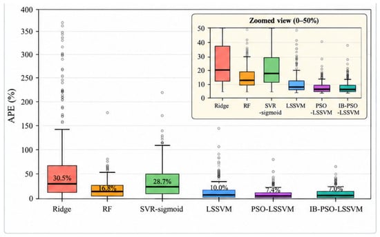
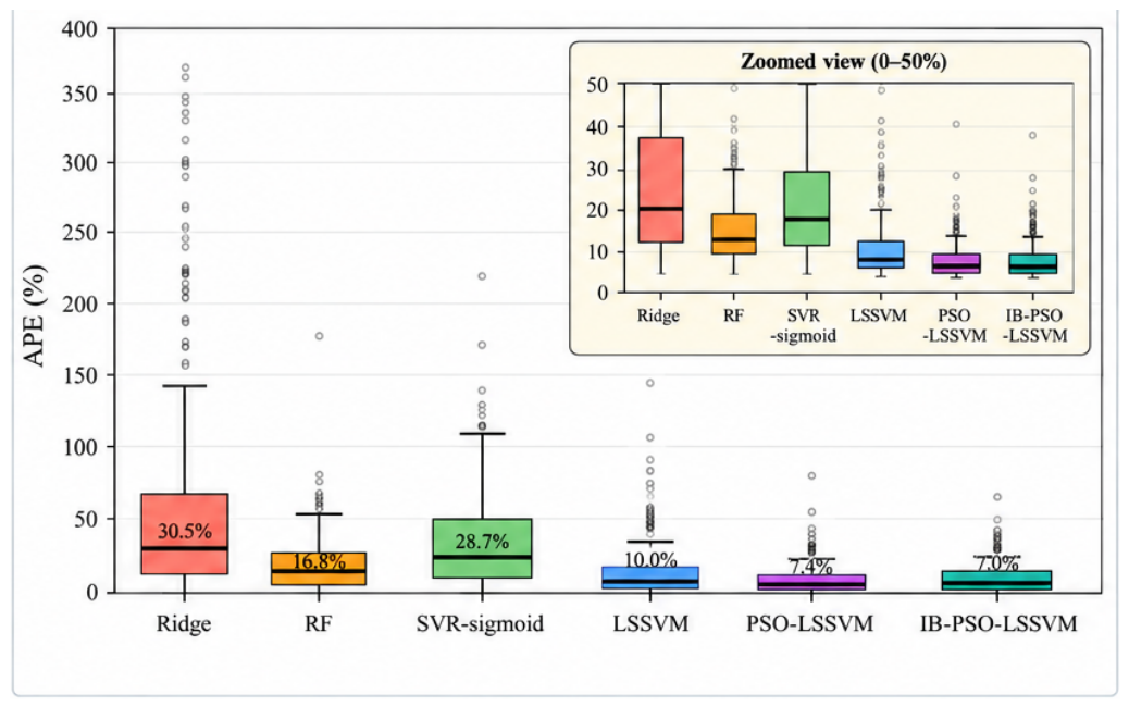
Although aggregate metrics summarize the average forecasting performance, they do not reveal how errors are distributed among individual projects. Figure 1 therefore presents box plots of the project-level absolute percentage errors (APEs) produced by the six models.

Figure 1. Distribution of absolute percentage errors (APE) across prediction models. Boxes span the inter-quartile range (IQR); whiskers extend to $1.5\times$ IQR; medians are annotated. The inset lists the maximum APE and standard deviation for each method.

As shown in Figure 1, conventional PSO-LSSVM achieves the lowest aggregate MAPE but produces a maximum observed APE of 84.80%. The corresponding maximum APE of the proposed method was 69.35%. The standard deviation of project-level APE also decreased from 9.7 to 9.2 percentage points. Larger maximum errors were observed for conventional LSSVM and random forest, reaching 225.91% and 178.79%, respectively.

The reduction in the maximum observed project-level error accompanied the improvement in cross-interval balance. However, the maximum individual APE was not directly included in the proposed objective; the worst-interval term was calculated from the mean error within each cost interval. The project-level result should therefore be interpreted as an empirical outcome of the selected model rather than as a guaranteed property of the objective.

5.4. Cross-Interval Forecasting Performance

Table 7 reports the forecasting performance of all evaluated models across the four cost intervals. For each model, the interval-specific MAPE values were calculated from the pooled outer-fold predictions. The standard deviation of the four interval-specific MAPE values and the worst-interval MAPE were also reported to evaluate cross-interval consistency.

Table 7. Interval-specific prediction accuracy comparison of prediction models.

Method	MAPE (%)
	Interval I	Interval II	Interval III	Interval IV	Standard Deviation
Ridge	59.01	56.09	55.56	64.15	3.41
Random Forest	20.06	19.62	18.79	39.02	8.47
SVR-sigmoid	28.31	17.03	44.07	68.15	19.18
Conventional LSSVM	15.77	15.41	14.07	19.60	2.37
Conventional PSO-LSSVM	10.03	8.94	8.09	13.60	1.91
Proposed Method	9.76	9.49	8.42	12.49	1.59

Note: Bold values indicate the best performance for each metric.

Among all models, the conventional PSO-LSSVM achieved the lowest MAPE in Intervals II and III, while the proposed interval-balanced PSO-LSSVM performed best in Intervals I and IV, where project costs are either low or high. No single model maintained the lowest error across all four intervals. This observation indicates that minimizing the global validation error does not necessarily produce consistent prediction performance across projects of different cost scales.

The benchmark models generally performed better in the middle-cost ranges (Intervals II and III), whereas their prediction errors increased at the extremes (Intervals I and IV). In contrast, the proposed method reduced the worst-interval MAPE from 13.60% to 12.49% and the standard deviation of interval-specific MAPE from 1.91 to 1.59, although this improvement came at the expense of slightly higher errors in Intervals II and III compared with conventional PSO-LSSVM. This trade-off is consistent with the motivation of group-aware optimization, which emphasizes worst-group performance rather than aggregate accuracy alone [45]. The present study extends this perspective to construction cost forecasting by incorporating interval-error dispersion and worst-interval penalties into PSO-LSSVM hyperparameter selection.

Based on consultations with engineering cost-management experts, an APE of 30% was adopted as a practical acceptability threshold for early-stage cost forecasting. As shown in Table 8, only 20 of the 440 project-level predictions generated by the proposed method had an APE greater than 30%. Thus, 420 predictions (95.45%) satisfied the practical acceptability threshold. The proposed method also produced the fewest predictions with APE values exceeding 10%, 30%, and 50% among the evaluated models. These results indicate that the proposed objective improved cross-interval balance while limiting large project-level prediction errors.

Table 8. Distribution of project-level absolute percentage errors across prediction models.

Method	APE > 10%	APE > 30%	APE > 50%	Maximum APE (%)
Ridge	352 (80.00%)	222 (50.45%)	149 (33.86%)	504.81
RF	298 (67.73%)	102 (23.18%)	30 (6.82%)	178.79
SVR-sigmoid	313 (71.14%)	153 (34.77%)	67 (15.23%)	239.55
LSSVM	220 (50.00%)	52 (11.82%)	20 (4.55%)	225.91
Conventional PSO-LSSVM	175 (39.77%)	28 (6.36%)	4 (0.91%)	84.80
Proposed Method	157 (35.68%)	20 (4.5%)	2 (0.45%)	69.35

Note: Bold values indicate the best performance for each metric.

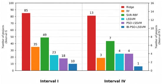
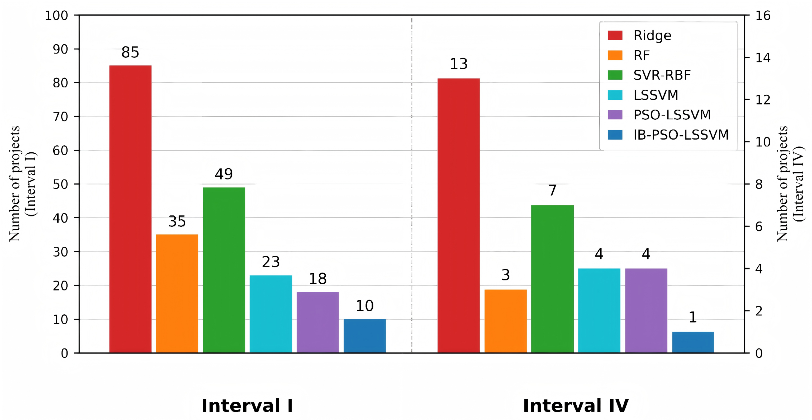
To further examine the practical implications for project budgeting, Figure 2 compares severe directional prediction errors in the lowest- and highest-cost intervals. In Interval I, which contains 211 projects, the proposed IB-PSO-LSSVM reduces the number of overestimations exceeding 30% from 18 to 10 compared with conventional PSO-LSSVM, representing a reduction of 44.4%. In Interval IV, which contains 42 projects, the number of underestimations exceeding 30% decreases from 4 to 1, representing a reduction of 75.0%. The proposed method achieves the fewest severe directional errors in both intervals among all six evaluated models. From a project budgeting perspective, reducing substantial overestimation of low-cost projects can help avoid excessive budget reservations, while reducing severe underestimation of high-cost projects can help mitigate potential funding shortfalls. These findings demonstrate that improved cross-interval prediction balance is accompanied by fewer severe, budgeting-relevant prediction errors, highlighting the practical value of the proposed method for early-stage project cost forecasting.

Figure 2. Number of projects with severe directional prediction errors.

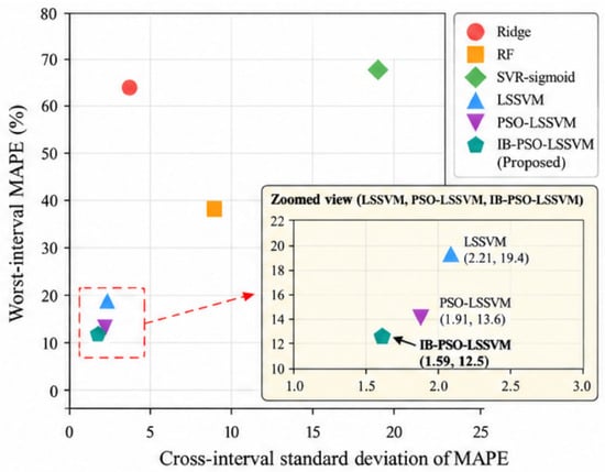
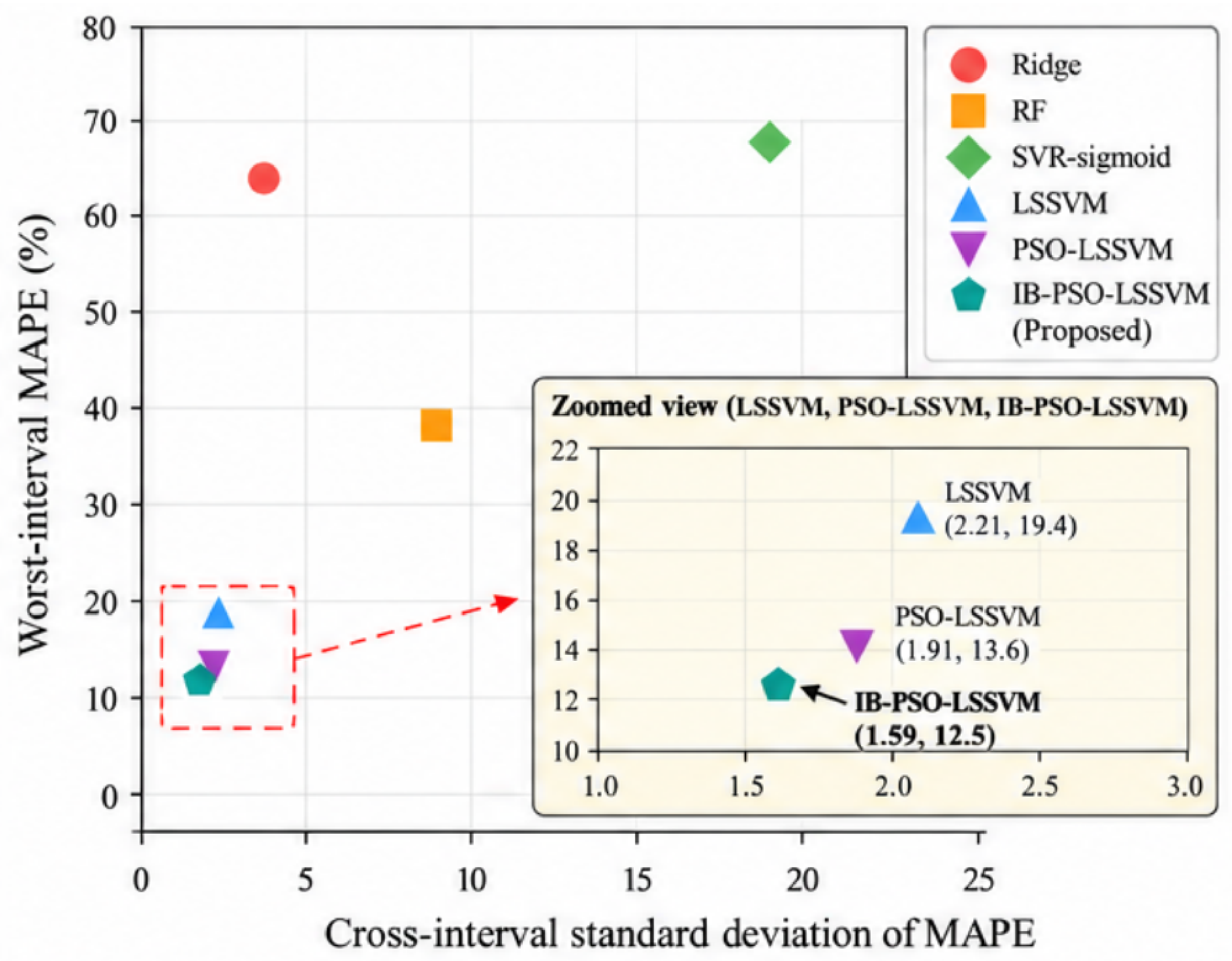
Figure 3 summarizes the trade-off between the standard deviation of interval-specific MAPE and the worst-interval MAPE. The proposed method occupies a more favorable position on these two balance-oriented indicators than the benchmark models. This improvement was obtained with small increases in the MAPE values of the two middle intervals and a more noticeable deterioration in aggregate RMSE. Accordingly, the results demonstrate improved cross-interval balance rather than an unqualified improvement in forecasting performance.

Figure 3. Cross-interval prediction balance of prediction models. The horizontal axis represents the standard deviation of interval-specific MAPE values; the vertical axis represents the worst-interval MAPE.

From a cost-management perspective, this trade-off may be relevant when poor performance within a less frequently represented cost range is considered more consequential than a small increase in average error. For example, project owners screening heterogeneous projects may prefer a model with fewer pronounced interval-level weaknesses, even when another model provides a lower aggregate RMSE. The preferred model nevertheless depends on the decision objective. Conventional PSO-LSSVM remains preferable when aggregate predictive accuracy is the primary criterion, whereas the proposed method is more suitable when performance consistency across project-cost ranges is explicitly valued.

5.5. Ablation Study

An ablation analysis was conducted to examine the individual contributions of the cross-interval dispersion term and the excess worst-interval term. Three PSO fitness functions were compared under the same nested cross-validation partitions and computational settings. The first objective, $J_1 = E_G$, represented conventional PSO-LSSVM and considered only the global prediction error. The second objective, $J_2 = E_G + \lambda B$, additionally penalized variation among the interval-specific errors. The complete objective, $J_3 = E_G + \lambda B + \mu W$, further penalized the excess error of the worst-performing interval.

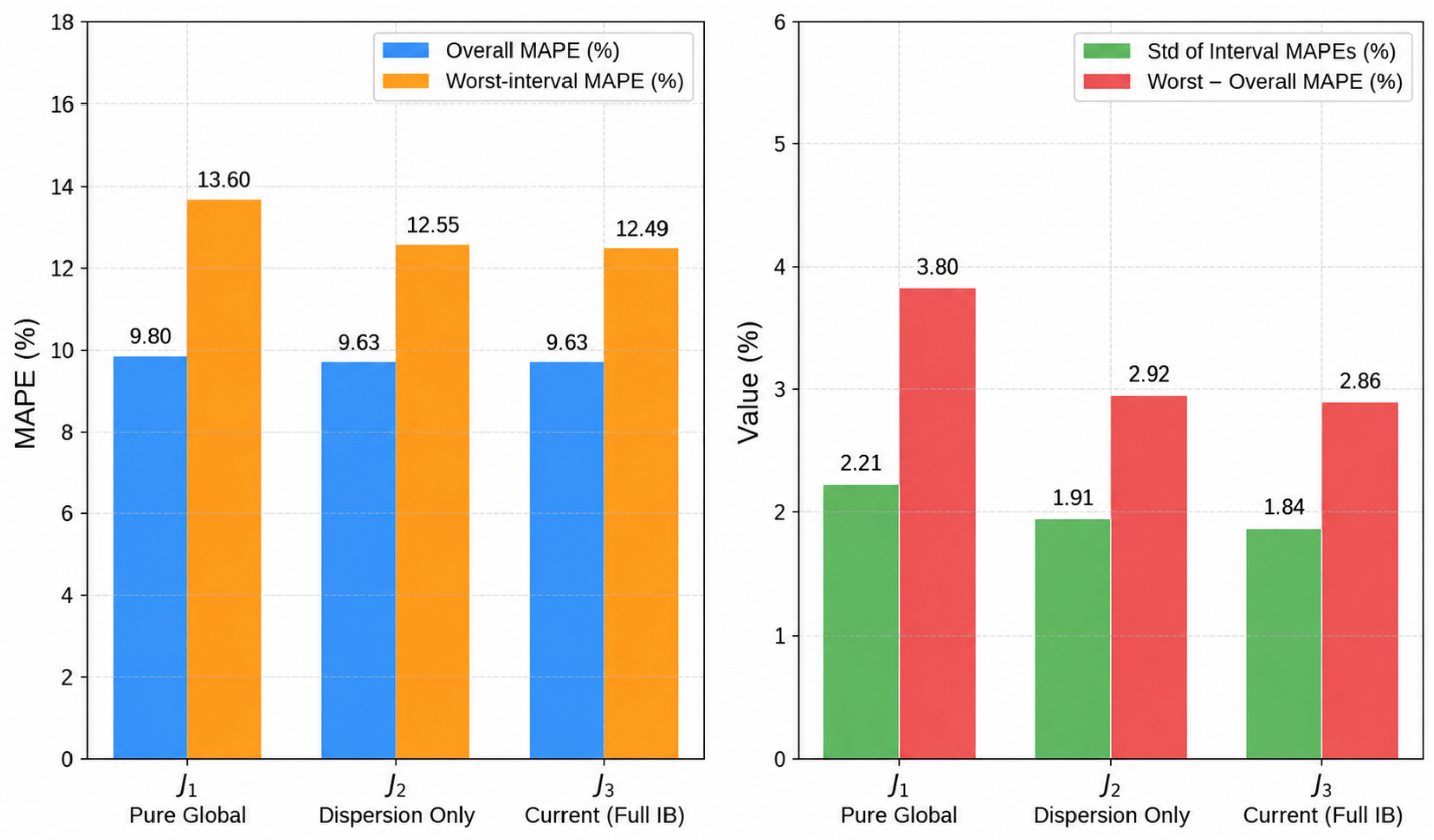
Table 9 presents the overall and cross-interval performance obtained under the three objective functions. When the global error was used alone, which is indeed the conventional PSO-LSSVM, the model achieved a worst-interval MAPE of 13.60%, while the cross-interval variations in prediction errors B and excess worst-interval error W were 2.21 and 3.80, respectively. When the term $\lambda B$ was added to the baseline objective $J_1 = E_G$, the overall MAPE increased slightly from 9.63% to 9.79%, while the worst-interval MAPE decreased from 13.60% to 12.55%, and B dropped from 2.21 to 1.91. This indicates that the balanced term effectively reduced the dispersion of interval-specific errors at the cost of a marginal increase in the global error.

Table 9. Ablation results for different PSO hyperparameter-selection objectives.

Objective	Overall MAPE	Worst-Interval MAPE (%)	B	W
$J_1 = E_G$	9.63	13.60	2.21	3.80
$J_2 = E_G + \lambda B$	9.79	12.55	1.91	2.92
$J_3 = E_G + \lambda B + \mu W$	9.80	12.49	1.84	2.86

When the worst-interval penalty $\mu W$ was further introduced to form the complete objective $J_3 = E_G + \lambda B + \mu W$, the overall MAPE remained virtually unchanged at 9.80%, whereas the worst-interval MAPE was further reduced to 12.49%, and W declined from 3.80 to 2.86. The reduction in W was accompanied by only a limited change in the global error. The complete objective therefore prevented the improvement in average interval consistency from being achieved while leaving one cost interval with a comparatively large prediction error.

The two interval-related components played distinct but complementary roles. The dispersion term B controlled the overall variation among interval-specific errors. However, because it summarizes deviations around the mean interval error, a relatively poor interval may still remain if the errors of the other intervals shift correspondingly. The term W directly addressed this limitation by penalizing the excess error of the worst-performing interval. Their joint inclusion resulted in the lowest cross-interval dispersion and worst-interval error among the three objective settings.

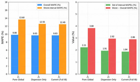
Figure 4 compares the overall error, cross-interval dispersion, worst-interval MAPE, and excess worst-interval error under the three objective functions. The addition of B and W gradually shifted the selected model from pure aggregate-error minimization toward a more balanced error profile. Although the complete objective did not necessarily produce the lowest $E_G$, it provided the most favorable combination of overall accuracy, cross-interval consistency, and worst-interval performance. These findings support the notion that the improved forecasting stability of the proposed method was attributable to the two added objective components rather than to PSO or LSSVM alone.

Figure 4. Comparison of overall MAPE, standard deviation of interval MAPEs, worst-interval MAPE, and excess worst-interval error across three objective functions: $J_1$ (Pure Global), $J_2$ (Dispersion Only), and $J_3$ (Current, Full IB).

To assess the statistical reliability of the observed improvements, a paired bootstrap analysis was conducted using the out-of-sample predictions of conventional PSO-LSSVM and the proposed method (shown in Table 10. The proposed method significantly reduced the worst-interval MAPE from 13.60% to 12.49% (one-sided p = 0.04), providing statistical evidence for improved prediction accuracy in the worst-performing cost interval. The standard deviation of interval-specific MAPE also decreased from 1.91 to 1.59, although this reduction was not statistically significant (p = 0.18). These findings indicate that the proposed method improves worst-interval prediction performance, while the evidence for a reduction in cross-interval error dispersion remains less conclusive.

Table 10. Paired bootstrap comparison of cross-interval prediction performance.

Performance Measure	Conventional PSO-LSSVM	Proposed Method	Improvement	95% CI	p-Value
Worst-interval MAPE (%)	13.60	12.49	1.11	$[-0.42, 1.32]$	0.04
Std. of intervall MAPEs	1.91	1.59	0.32	$[-0.24, 0.57]$	0.18

Note: Improvements are expressed in percentage points. The 95% confidence intervals are two-sided. The p-values are obtained from one-sided paired bootstrap tests, with the alternative hypothesis that the proposed method achieves a lower error than conventional PSO-LSSVM.

6. Conclusions

This study developed an interval-balanced PSO-LSSVM framework for small-sample cost forecasting of overhead transmission line construction projects. The framework extends conventional PSO-LSSVM hyperparameter optimization by jointly considering global prediction error, cross-interval error dispersion, and the excess error of the worst-performing interval. Cost intervals were constructed from the observed training costs using one-dimensional clustering, with the number of intervals selected by the silhouette coefficient. Nested cross-validation was used to separate preprocessing, interval construction, hyperparameter selection, and out-of-sample evaluation.

The results show that conventional PSO-LSSVM achieved the best aggregate accuracy, with an overall MAPE of 9.63%. The proposed method achieved a comparable overall MAPE of 9.80%, while outperforming the other benchmark models in terms of cross-interval balance. In particular, the proposed method obtained the lowest standard deviation of interval-specific MAPE values (1.59) and the lowest worst-interval MAPE (12.49%) among the evaluated models. It performed best in the lowest- and highest-cost intervals, whereas conventional PSO-LSSVM performed slightly better in the two middle-cost intervals. This result illustrates the trade-off between aggregate accuracy and more consistent prediction performance across heterogeneous project-cost ranges.

From a construction cost-management perspective, the framework provides a means of incorporating cost-range consistency into model selection without requiring separate forecasting models for individual project groups. It may therefore assist early-stage budget preparation, project screening, and preliminary cost review when historical observations are limited and unevenly distributed. The predictions should nevertheless be used as decision-support information rather than as substitutes for detailed quantity-based estimates or professional engineering review.

This study has several limitations. The empirical analysis was based on 440 projects obtained from a limited number of organizations within one regional context. The selected predictors, cost structure, and interval boundaries may not represent other regions or types of construction projects. Therefore, the observed improvement in cross-interval prediction consistency should be interpreted within the scope of the present dataset and experimental setting. In addition, the interval definitions depend on the observed training-cost distribution, and the selected penalty weights reflect the trade-off adopted in the present study. Future research should validate the framework using larger, multi-regional, and cross-organizational datasets; examine the stability of the selected intervals and penalty weights; and compare alternative clustering methods, balance-oriented objectives, and hyperparameter optimization algorithms.

References

- Gao, Y.; Antwi-Afari, M.F.; Huang, Y.; Chen, Z.S.; Manzoor, B. Artificial Intelligence in Construction Project Management: A Systematic Literature Review of Cost, Time, and Safety Management. Buildings 2026, 16, 1061. [Google Scholar] [CrossRef] [Scilit]
- Habib, O.; Abouhamad, M.; Bayoumi, A. Ensemble Learning Framework for Forecasting Construction Costs. Autom. Constr. 2025, 170, 105903. [Google Scholar] [CrossRef] [Scilit]
- Padala, S.P.S.; Goyal, A. Early Stage Cost Prediction Model for Indian Building Construction Projects Using Artificial Neural Networks. J. Financ. Manag. Prop. Constr. 2025, 30, 377–397. [Google Scholar] [CrossRef] [Scilit]
- Li, Y.; Chang, Y. Infrastructure Investments for Power Trade and Transmission in ASEAN + 2: Costs, Benefits, Long-Term Contracts and Prioritized Developments. Energy Econ. 2015, 51, 484–492. [Google Scholar] [CrossRef] [Scilit]
- Li, B.; Hu, Q.; Guo, R.; Hu, J.; Fen, Z.; Hua, X.; Zhu, T.; Yuan, Y. A Review of the Developments in Capacity-Uprating Conductors for Overhead Transmission Lines. Coatings 2025, 15, 1203. [Google Scholar] [CrossRef] [Scilit]
- Lowe, D.J.; Emsley, M.W.; Harding, A. Predicting Construction Cost Using Multiple Regression Techniques. J. Constr. Eng. Manag. 2006, 132, 750–758. [Google Scholar] [CrossRef] [Scilit]
- Hwang, S. Dynamic Regression Models for Prediction of Construction Costs. J. Constr. Eng. Manag. 2009, 135, 360–367. [Google Scholar] [CrossRef] [Scilit]
- Bayram, S.; Al-Jibouri, S. Efficacy of Estimation Methods in Forecasting Building Projects’ Costs. J. Constr. Eng. Manag. 2016, 142, 05016012. [Google Scholar] [CrossRef] [Scilit]
- Elmousalami, H.; Elshaboury, N.; Ibrahim, A.H.; Elyamany, A.H. Bayesian Optimized Ensemble Learning System for Predicting Conceptual Cost and Construction Duration of Irrigation Improvement Systems. KSCE J. Civ. Eng. 2025, 29, 100014. [Google Scholar] [CrossRef] [Scilit]
- Das, P.; Kashem, A.; Hasan, I.; Islam, M. A Comparative Study of Machine Learning Models for Construction Costs Prediction with Natural Gradient Boosting Algorithm and SHAP Analysis. Asian J. Civ. Eng. 2024, 25, 3301–3316. [Google Scholar] [CrossRef] [Scilit]
- Karadimos, P.; Anthopoulos, L. A Taxonomy of Machine Learning Techniques for Construction Cost Estimation. Innov. Infrastruct. Solut. 2024, 9, 420. [Google Scholar] [CrossRef] [Scilit]
- Ke, T.; Zhang, L.; Ge, X.; Lv, H.; Li, M. Construct a Robust Least Squares Support Vector Machine Based on Lp-Norm and L∞-Norm. Eng. Appl. Artif. Intell. 2021, 99, 104134. [Google Scholar] [CrossRef] [Scilit]
- Sing, M.C.P.; Ma, Q.; Gu, Q. Improving Cost Contingency Estimation in Infrastructure Projects with Artificial Neural Networks and a Complexity Index. Appl. Sci. 2025, 15, 3519. [Google Scholar] [CrossRef] [Scilit]
- Lee, J.G.; Lee, H.S.; Park, M.; Seo, J. Early-Stage Cost Estimation Model for Power Generation Project with Limited Historical Data. Eng. Constr. Archit. Manag. 2022, 29, 2599–2614. [Google Scholar] [CrossRef] [Scilit]
- Zhao, X.h.; Miao, X.j.; Zhang, Z.g.; Zheng, H. Research on Prediction Method of Reasonable Cost Level of Transmission Line Project Based on PCA-LSSVM-KDE. Math. Probl. Eng. 2019, 2019, 1649086. [Google Scholar] [CrossRef] [Scilit]
- Son, H.; Kim, C.; Kim, C. Hybrid Principal Component Analysis and Support Vector Machine Model for Predicting the Cost Performance of Commercial Building Projects. Autom. Constr. 2012, 27, 60–66. [Google Scholar] [CrossRef] [Scilit]
- Yun, S. Performance Analysis of Construction Cost Prediction Using Neural Network for Multioutput Regression. Appl. Sci. 2022, 12, 9592. [Google Scholar] [CrossRef] [Scilit]
- Darko, A.; Glushakova, I.; Boateng, E.B.; Chan, A.P.C. Using Machine Learning to Improve Cost and Duration Prediction Accuracy in Green Building Projects. J. Constr. Eng. Manag. 2023, 149, 04023061. [Google Scholar] [CrossRef] [Scilit]
- Jassim, H.S.H.; Hasan, M.F.; Altaee, M.J.; Gamil, Y. A Model for Preliminary Cost Estimation in Buildings Construction Projects. Front. Built Environ. 2025, 11, 1359777. [Google Scholar] [CrossRef] [Scilit]
- Li, X.; Han, K.; Liu, W.; Wang, T.; Li, C.; Yan, B.; Hao, C.; Xian, X.; Yang, Y. Prediction Model of Farmland Water Conservancy Project Cost Index Based on PCA–DBO–SVR. Sustainability 2025, 17, 2702. [Google Scholar] [CrossRef] [Scilit]
- Gharaibeh, H.M. Managing the Cost of Power Transmission Projects: Lessons Learned. J. Constr. Eng. Manag. 2013, 139, 1063–1067. [Google Scholar] [CrossRef] [Scilit]
- Pham, H.; Luu, T.V.; Kim, S.Y.; Vien, D.T. Assessing the Impact of Cost Overrun Causes in Transmission Lines Construction Projects. KSCE J. Civ. Eng. 2020, 24, 1029–1036. [Google Scholar] [CrossRef] [Scilit]
- Ye, K.; Qiu, S.; Lin, J.; Zhu, X.; Ye, M. A Study on the Identification of Cost-Sensitive Factors in the Budgeting Stage of Power Transmission and Transformation Projects. In Proceedings of the 2025 International Conference on Power Systems, Smart Grid, and Artificial Intelligence (PSGAI), Xining, China, 26–28 December 2025; pp. 79–83. [Google Scholar] [CrossRef] [Scilit]
- Yi, T.; Zheng, H.; Tian, Y.; Liu, J.P. Intelligent Prediction of Transmission Line Project Cost Based on Least Squares Support Vector Machine Optimized by Particle Swarm Optimization. Math. Probl. Eng. 2018, 2018, 5458696. [Google Scholar] [CrossRef] [Scilit]
- Zhao, X.; Ni, T.; Miao, X.; Guo, L. Research on the Determination of Reasonable Cost Range of Power Grid Production Technological Transformation Project. IOP Conf. Ser. Earth Environ. Sci. 2020, 571, 012036. [Google Scholar] [CrossRef] [Scilit]
- Peng, S.; Zuo, Y.; Li, X.; Zhao, M.; Li, B. Cost Prediction for Power Transmission and Transformation Projects in High-Altitude Regions Based on a Hybrid Deep-Learning Algorithm. Processes 2025, 13, 2092. [Google Scholar] [CrossRef] [Scilit]
- Shi, Q.; Le, Y.; Gu, C.; Geng, Y. Research on Dynamic Cost Prediction Method for Power Technology Upgrading Projects Based on Improved Transformer Neural Network. Sci. Rep. 2026, 16, 28818. [Google Scholar] [CrossRef] [Scilit] [PubMed]
- Niu, D.; Zhao, W.; Li, S.; Chen, R. Cost Forecasting of Substation Projects Based on Cuckoo Search Algorithm and Support Vector Machines. Sustainability 2018, 10, 118. [Google Scholar] [CrossRef] [Scilit]
- Lin, T.; Yi, T.; Zhang, C.; Liu, J. Intelligent Prediction of the Construction Cost of Substation Projects Using Support Vector Machine Optimized by Particle Swarm Optimization. Math. Probl. Eng. 2019, 2019, 7631362. [Google Scholar] [CrossRef] [Scilit]
- Wang, H.; Liang, Y.; Ding, W.; Niu, D.; Li, S.; Wang, F. The Improved Least Square Support Vector Machine Based on Wolf Pack Algorithm and Data Inconsistency Rate for Cost Prediction of Substation Projects. Math. Probl. Eng. 2020, 2020, 6663006. [Google Scholar] [CrossRef] [Scilit]
- Xu, X.; Peng, L.; Ji, Z.; Zheng, S.; Tian, Z.; Geng, S. Research on Substation Project Cost Prediction Based on Sparrow Search Algorithm Optimized BP Neural Network. Sustainability 2021, 13, 13746. [Google Scholar] [CrossRef] [Scilit]
- Wang, C.; Zhang, H. An Explainable Machine Learning Perspective: Substation Cost Prediction Using the GSA–XGBoost Optimization Framework. Electr. Power Syst. Res. 2026, 261, 113456. [Google Scholar] [CrossRef] [Scilit]
- Wu, Z.; Liu, M.; Ma, G. A Machine Learning-Based Two-Stage Integrated Framework for Cost Reasonableness Prediction of Green Building Projects. J. Build. Eng. 2025, 100, 111733. [Google Scholar] [CrossRef] [Scilit]
- Abdelsalam, M.; Ashmawi, A.; Nguyen, P.H.D. AI-Driven Automation of Construction Cost Estimation: Integrating BIM with Large Language Models. Buildings 2026, 16, 485. [Google Scholar] [CrossRef] [Scilit]
- Ribeiro, R.P.; Moniz, N. Imbalanced Regression and Extreme Value Prediction. Mach. Learn. 2020, 109, 1803–1835. [Google Scholar] [CrossRef] [Scilit]
- Yang, Y.; Zha, K.; Chen, Y.; Wang, H.; Katabi, D. Delving into Deep Imbalanced Regression. In Proceedings of the 38th International Conference on Machine Learning, Online, 18–24 July 2021; pp. 11842–11851. [Google Scholar]
- Avelino, J.G.; Cavalcanti, G.D.C.; Cruz, R.M.O. Resampling Strategies for Imbalanced Regression: A Survey and Empirical Analysis. Artif. Intell. Rev. 2024, 57, 82. [Google Scholar] [CrossRef] [Scilit]
- Steininger, M.; Kobs, K.; Davidson, P.; Krause, A.; Hotho, A. Density-Based Weighting for Imbalanced Regression. Mach. Learn. 2021, 110, 2187–2211. [Google Scholar] [CrossRef] [Scilit]
- Ren, J.; Zhang, M.; Yu, C.; Liu, Z. Balanced MSE for Imbalanced Visual Regression. In Proceedings of the IEEE/CVF Conference on Computer Vision and Pattern Recognition, New Orleans, LA, USA, 19–24 June 2022; pp. 7926–7935. [Google Scholar] [CrossRef] [Scilit]
- Liang, R.; Zhang, G.; Zhang, K.; Lei, Z.; Zhang, S. Bilateral-Branch Network for Imbalanced Visual Regression. In Proceedings of the 2022 IEEE 34th International Conference on Tools with Artificial Intelligence (ICTAI), Macao, China, 31 October–2 November 2022; pp. 140–147. [Google Scholar] [CrossRef] [Scilit]
- Gong, Y.; Mori, G.; Tung, F. RankSim: Ranking Similarity Regularization for Deep Imbalanced Regression. In Proceedings of the 39th International Conference on Machine Learning Research, Baltimore, MD, USA, 17–23 July 2022; pp. 7634–7649. [Google Scholar]
- Keramati, M.; Meng, L.; Evans, R.D. ConR: Contrastive Regularizer for Deep Imbalanced Regression. In Proceedings of the Twelfth International Conference on Learning Representations, Vienna, Austria, 7–11 May 2024; Available online: https://openreview.net/forum?id=RIuevDSK5V (accessed on 28 October 2026).
- Wang, Z.; Wang, H. Variational Imbalanced Regression: Fair Uncertainty Quantification via Probabilistic Smoothing. In Proceedings of the Advances in Neural Information Processing Systems, New Orleans, LA, USA, 10–16 December 2023; pp. 30429–30452. [Google Scholar] [CrossRef] [Scilit]
- Asgarkhani, N.; Kazemi, F.; Jankowski, R. Machine-Learning Based Tool for Seismic Response Assessment of Steel Structures Including Masonry Infill Walls and Soil-Foundation-Structure Interaction. Comput. Struct. 2025, 317, 107918. [Google Scholar] [CrossRef] [Scilit]
- Sagawa, S.; Koh, P.W.; Hashimoto, T.B.; Liang, P. Distributionally Robust Neural Networks for Group Shifts: On the Importance of Regularization for Worst-Case Generalization. In Proceedings of the International Conference on Learning Representations, Online, 26 April–1 May 2020; Available online: https://openreview.net/forum?id=ryxGuJrFvS (accessed on 28 October 2026).
Disclaimer/Publisher’s Note: The statements, opinions and data contained in all publications are solely those of the individual author(s) and contributor(s) and not of MDPI and/or the editor(s). MDPI and/or the editor(s) disclaim responsibility for any injury to people or property resulting from any ideas, methods, instructions or products referred to in the content. |
© 2026 by the authors. Licensee MDPI, Basel, Switzerland. This article is an open access article distributed under the terms and conditions of the Creative Commons Attribution (CC BY) license.