


Abstract
Vertical displacement monitoring during super high-rise construction requires long stand-off distances and oblique imaging, for which conventional Sampling Moiré Method (SMM) processing suffers projection-scale bias and camera-support drift. This study presents a field-oriented workflow combining intrinsic camera calibration, in-situ marker-plane geometry, SMM phase extraction, and a fixed reference channel. The oblique-view degradation is quantified by a dimensionless period-non-uniformity index that separates uniform projection-scale error from spatial period-gradient error and partitions the tilt/distance space into design zones. Numerical and physical tilt sweeps show that homography rectification and adaptive local sampling keep the RMSE below 0.3 mm up to , where the uncorrected measurement reaches approximately 2 mm; these two strategies are intended for caution/danger-zone geometries, whereas the field workflow used a locally estimated scale correction, consistent with the design case m (). A single-run outdoor 50 m three-point experiment shows that differencing against a fixed reference marker reduces the RMSE by 45.7% and approximately 31% at two moving markers. In two non-simultaneous field programmes, the laser rangefinder and corrected SMM were evaluated independently against the same 1–10 mm prescribed sequence. Their ten-level MAE/RMSE values were 0.280/0.303 mm and 0.165/0.207 mm, respectively. Each programme reports accuracy within its own installation and loading arrangement. The results provide short-term evidence for traceable, long-distance oblique-view displacement monitoring during construction.
1. Introduction
The structural health monitoring (SHM) of large-scale infrastructure is important for construction safety and long-term operational stability. In super high-rise buildings, vertical deformation control is driven by the cumulative effects of material creep and construction loads, while lateral wind and seismic actions motivate complementary monitoring of dynamic response. Studies of mega-subcontrolled, mega-frame, and core-tube–outrigger systems show that displacement and acceleration responses depend strongly on the structural configuration, damping, excitation type, and modeling uncertainty [1,2,3]. The present study focuses on construction-stage quasi-static vertical displacement, with prospective wind- and seismic-response applications discussed in Section 6. Wang and Xiao [4] highlighted the importance of deformation control measures during the construction of asymmetric high-rise buildings, and long-term vision-based displacement monitoring of high-rise structures under field conditions has been reported [5]. Zhou et al. [6] proposed an adaptive unscented Kalman filter to improve axial deformation prediction. While ground-based radar and LiDAR can achieve submillimeter accuracy for dynamic deformation [7], these methods are often constrained by high equipment costs, low sampling frequencies, or the inability to perform real-time continuous measurement.
To overcome the limitations of contact-based or point-wise sensors, computer vision-based SHM has emerged as an effective alternative. As reviewed by Dong and Catbas [5], vision-based methods offer non-contact, long-distance, and cost-effective advantages for both local damage detection and global displacement measurement. Central to these geometric measurements is robust camera calibration. Zhang [8] established the foundational flexible method for planar camera calibration, which remains widely used in photogrammetry, and later extended the calibration framework to one-dimensional objects [9], while Zhang et al. [10] further optimized calibration robustness using single-image 2.5D targets. Recent reviews have summarized close-range photogrammetric techniques for structural monitoring [5]. Among vision-based techniques, the Sampling Moiré Method (SMM) has gained significant attention for its high precision and computational efficiency. SMM allows for the retrieval of displacement fields from periodic patterns with sub-pixel accuracy. Recent theoretical work by Sur et al. [11] has rigorously characterized the measurement resolution and bias of SMM, proving its equivalence to localized spectrum analysis under certain conditions. SMM has been applied to measure slip activities in superalloys [12], characterize heat-resistant gratings at high temperatures [13], and correct distortion in Scanning Electron Microscopy images [14], as well as for misalignment measurement in electron beam lithography [15] and microscopic cooling-deformation measurement in composite materials [16]. Complementary mechanical studies have characterized the deformation behavior of ancient timber structural components [17], and innovative sensor designs such as optical cantilevers [18] and three-axis force plates [19] have also integrated SMM for high-resolution sensing.
Recent developments have further expanded the applicability of SMM to challenging dynamic and optical conditions. To address the difficulty of measuring slender structures, Sun et al. [20] developed a high-speed displacement measurement technique for slender structures, and Qi et al. [21] extended the method to residual stress measurement. For consumer-grade applications, Gao et al. [22] validated the feasibility of using smartphone lenses for displacement measurement. In terms of optical configurations, Ri et al. [23] achieved ultra-wide-field measurement using fisheye lenses, while He et al. [24] enhanced 3D structured illumination microscopy by combining binary encoding with SMM. Additionally, Ri et al. [25] introduced image scaling techniques for accurate strain measurement in composite materials undergoing large deformations.
Applying SMM to vertical deformation monitoring of super high-rise buildings presents four practical challenges: (1) Long observation distance—construction sites typically require monitoring at distances of 50–100 m, far exceeding the laboratory and short-range conditions in most SMM applications; (2) Oblique viewing angle—the geometric constraints on construction sites often prevent the camera from being positioned perpendicular to the target, leading to perspective distortion that varies spatially across the grating marker; (3) Field deployment—practical implementation requires robust camera calibration, stable marker installation, and paired multi-camera acquisition under uncontrolled environmental conditions; and (4) Insufficient systematic validation—few studies have compared SMM against established construction-site instruments such as laser rangefinders under representative field conditions. Ri et al. [26] noted that camera motion is a significant source of error and proposed advanced image stabilization to compensate for it; however, their approach addresses post-acquisition image stability rather than the geometric projection bias introduced by oblique viewing. Jiang et al. [27] proposed a calibration-free method to automatically detect camera direction for large structure inspection, which avoids explicit intrinsic calibration but does not correct the resulting scale distortion. Shangguan et al. [28] investigated oblique imaging laws to compensate for displacement errors in large-scale bridges using a CCD Moiré formulation; their correction is based on an empirical angular factor rather than a calibrated homography, whereas the present work derives the local scale factor from the field-marker pose estimated during calibration. Multi-camera vision systems have also been developed for simultaneous multi-point field measurement [5]. However, a systematic integration of camera calibration, perspective rectification, and differential measurement for long-distance oblique-view SMM has not been reported.
This study develops a field-oriented displacement measurement configuration that integrates SMM with two complementary corrections: a geometric scale correction for the obliquely viewed marker and a fixed reference channel for estimating apparent drift. The oblique-view degradation is quantified through a dimensionless period-non-uniformity index that partitions the tilt-angle and relative-distance space into design zones, and both the geometric correction and the reference channel are validated by dedicated controlled experiments in addition to the field trial. The effectiveness of reference-channel correction depends on the similarity of the two cameras’ disturbance responses. The overall processing pipeline is illustrated in Figure 1. Related SHM research has used operational modal analysis and stochastic subspace identification to track temperature and retrofitting effects from synchronized structural responses; these applications motivate dynamic extensions beyond the present quasi-static scope [29,30,31,32]. A controlled experiment at an observation distance of approximately 58 m, with prescribed vertical displacements of 1–10 mm, evaluates the internal consistency and short-term engineering feasibility of the workflow, with laser ranging included as an engineering comparison against the prescribed-displacement reference.
Figure 1.
Overall processing pipeline. Camera calibration supplies the intrinsic and distortion parameters; the field-marker pose used in is estimated from the installed marker. In the notation used here, is the physical pitch, N is the number of phase steps, and k is the step index. Reference-channel correction is applied after the two single-channel displacement outputs.
The method combines separate estimates of camera intrinsics and installed-marker pose with a signed reference-channel response model. The dimensionless index guides the choice between local-scale correction and spatial rectification. Numerical and physical tilt sweeps evaluate the geometric correction, while channel-resolved displacement results quantify accuracy in the controlled field and outdoor reference-channel experiments.
The intended application is controlled vertical-displacement monitoring during construction at locations with a stable line of sight and an installed periodic marker. Geometric normalization and reference observation extend phase-based SMM measurement to the long-distance, oblique-view conditions encountered on building sites.
2. Principle of the Sampling Moiré Method
The Sampling Moiré Method (SMM) extracts displacement from the phase change of a periodic marker. A camera records a rectangular or approximately sinusoidal grating, and digital sampling and interpolation generate a phase-shifted Moiré sequence.
2.1. Grating Signal and Digital Moiré Formation
After averaging in the direction parallel to the fringes, a one-dimensional intensity signal can be written as
where i is an image coordinate, and are the local modulation and background intensity, respectively, is the grating pitch in image pixels, and is the initial phase. The symbol denotes an image pitch in this section; the physical marker pitch is denoted by below.
The one-dimensional representation is obtained by directional averaging within a two-dimensional region of interest (ROI). For vertical displacement, the grating orientation is chosen so that motion changes the phase in the measurement direction. Pixel values are averaged along the fringe direction, which suppresses uncorrelated sensor noise while retaining the periodic component. A low-pass or mean filter may then be used to reduce printing texture and background variation. The rectangular printed grating contains higher harmonics; mild optical defocus and numerical filtering attenuate those harmonics so that the fundamental component in Equation (1) dominates. The resulting fundamental component supports use of the sinusoidal phase model with rectangular printed markers.
If the digital sampling interval is pixels, the ideal difference-frequency Moiré pitch is
The principle follows from the difference-frequency relationship. Equation (2) also shows why the sampling interval cannot be selected independently of the captured image: if is too close to , the synthetic pitch grows large relative to the ROI; because the phase is recovered per pixel from the N-step resampled sequence, a large mainly reduces the spatial phase gradient available to the estimator; if the mismatch is too large, the resampled fringes become too fine for stable phase extraction.
Sampling parameters are selected in image space using the dominant ROI period. The integer interval is chosen near that period, and the resulting synthetic pitch is assessed against the usable ROI and the spatial estimator’s ability to resolve the phase gradient. The recorded parameter set comprises , , , ROI dimensions and filtering bandwidth for each camera.
2.2. Phase Extraction and Displacement Conversion
An N-step phase-shifted Moiré sequence may be represented as
where is the phase-step index and is the number of phase steps. The wrapped Moiré phase is evaluated with a complex argument, equivalent to a two-argument arctangent:
where . This notation separates the phase-step index k from the number of phase steps N and avoids the quadrant ambiguity of a one-argument inverse tangent.
In digital SMM, the N phase steps are generated from the same recorded grating image by changing the sampling origin and interpolating the missing pixels. Each image therefore provides all N computational phase steps.
For two states recorded before and after marker motion, the wrapped phase difference is
After phase unwrapping where required, the marker displacement in a geometrically normalized marker coordinate system is
where is the physical grating pitch and is expressed in the normalized marker coordinates. The local-scale route converts the apparent channel displacement using Equation (16); its uncertainty model is defined in Section 5.7.
For a spatial ROI containing valid phase at M pixels, a robust channel result can be formed from the median or a weighted mean of . A useful weight is proportional to the local modulation amplitude obtained from the same complex phase sum. Pixels near marker edges, saturated regions, and low-modulation areas should be masked before aggregation. Spatial aggregation produces one channel displacement for each image.
2.3. Processing Parameters and Quality Control
The field marker used in this study had a physical pitch of 98 mm and dimensions of , corresponding to approximately 5.1 physical grating periods across the marker. The image pitch , sampling interval , and phase-step number N are processing quantities selected from the captured ROI. The ROI dimensions, filtering bandwidth and sampling parameters jointly define each camera’s phase estimator.
The complete single-image processing order is: (1) undistort the raw image using the fixed intrinsic calibration; (2) identify or propagate the marker ROI; (3) rectify the ROI to marker coordinates or evaluate its local geometric scale; (4) estimate the image period and apply the recorded SMM sampling parameters; (5) calculate wrapped phase and modulation; (6) mask invalid pixels and unwrap the phase change; and (7) convert the spatially aggregated phase difference to physical displacement. Performing rectification before the image-period selection is important because an oblique raw image can have a period that varies across the ROI. The resulting channel displacement is then passed to the two-camera reference correction described in Section 5.
Processing quality can be assessed through three quantities: compatibility of the synthetic pitch with the ROI, spatial gradients in the phase residual after removal of the ROI mean, and consistency of the corrected-to-apparent displacement ratio with the local geometric scale. Residual gradients may indicate incomplete perspective normalization or marker warping. These checks complement image-level coordinate and sign verification.
2.4. Practical Constraints and Validity Conditions
The processing equations are applied subject to the following conditions:
- The phase-shifting sequence requires , non-zero local modulation, and a sampling interval . The synthetic pitch is assessed against the usable ROI and the selected spatial estimator; phase recovery from the per-pixel resampled sequence depends on the estimator’s ability to resolve the spatial phase gradient.
- Pixels affected by saturation, marker edges, occlusion, or low modulation are excluded before phase aggregation. Nearest-branch phase unwrapping requires the physical phase increment between adjacent valid samples to remain below ; larger increments require additional information to determine the integer multiples of .
- A planar homography requires at least four non-collinear correspondences with a non-degenerate image configuration. Marker warping, changing focus, or motion of either camera or marker after calibration invalidates the stored mapping.
- The local scale approximation is used when the analyzed ROI is small and remains in the model-defined safe zone. In caution/danger-zone operation, full spatial mapping or adaptive local sampling should be evaluated, particularly for spatial or asymmetric valid ROIs, together with the same signal-quality masks.
The field marker contains approximately 5.1 periods because a coarser pitch improves long-range visibility while retaining several cycles for phase aggregation. To quantify the resulting trade-off, Figure 2 varies the physical count from 3 to 10 in a fixed-width synthetic ROI, with identical normalized illumination gradient and sensor noise in 300 Monte-Carlo realizations. At the field count, the simulated displacement RMSE is approximately 0.08–0.09 mm depending on the edge mask, compared with approximately 0.12–0.14 mm for three periods and 0.04 mm for ten periods. Thus, 5.1 periods is a practical visibility–robustness compromise for the tested installation; installations permitting a larger marker or finer resolvable pitch should retain more usable periods.
Figure 2.
Numerical sensitivity of phase-derived displacement to the number of physical grating periods in a fixed-width ROI. Curves show RMSE over 1–5 mm displacements for three edge-mask widths (the fraction of the ROI width trimmed at each side) under 300 noise realizations; the dashed line marks the 5.1-period field marker. Illumination and noise settings are held constant across period counts.
3. Calibration and Oblique-View Correction
The geometric workflow comprises intrinsic camera calibration and installed-marker mapping. Checkerboard images determine the intrinsic matrix and lens-distortion coefficients; correspondences on the installed grating determine its in-situ pose or homography. Each stage uses the geometry of its own target. The following analysis relates oblique imaging to the choice of correction strategy.
3.1. Oblique Imaging Mechanism and Period Non-Uniformity
Consider a planar marker of width W whose center lies at optical-axis depth D from the camera, tilted by an angle about the vertical axis so that the marker normal forms the angle with the optical axis. A marker coordinate x along the tilt direction has depth , and its image coordinate under the pinhole model is
where f is the focal length in pixels. The local image-space grating period therefore varies across the field of view:
Equation (8) contains two distinct error mechanisms. The first is the uniform projection-scale factor at the marker center, which scales every apparent displacement by and is corrected by the local factor in Equation (16). The second is the spatial non-uniformity of the period, which violates the constant-frequency assumption underlying the fixed sampling interval of conventional SMM. Quantifying the second mechanism requires a dimensionless index. Defining the relative distance , we use the relative depth variation across the marker as a dimensionless period-non-uniformity index,
which defines a design map: is controlled only by the tilt angle and the relative distance. The corresponding edge-to-edge period ratio is . The projection requires and . The derivation assumes that the tilt axis is perpendicular to the measurement direction; when the measurement direction lies in the tilt plane (e.g., vertical displacement observed by an elevated camera), the same analysis applies with x taken along that direction. Figure 3 partitions the plane into a safe zone (), in which the imaging geometry is effectively affine and a local scale model may be used; a caution zone (), in which the spatial gradient should be checked; and a danger zone (), in which full geometric rectification or adaptive sampling is recommended, particularly for spatial or asymmetric ROIs. Representative simulated grating appearances at four tilt angles are shown in Figure 4.
Figure 3.
Period non-uniformity as a function of tilt angle and relative distance. Dashed and solid contours mark the 1% and 5% zone boundaries. The filled square marks the uniaxial validation geometry of Section 4.3 ( mm marker, , ), which falls in the danger zone. The upward arrow indicates the field design case ( m, , ) above the plotted range; its lies in the safe zone.
Figure 4.
Simulated imaging appearance of the matrix-array marker at increasing tilt angle. The marker pattern consists of dark square blocks arranged in a grid, as used in the field installation; with growing tilt the column spacing becomes progressively non-uniform (near-side columns widen, far-side columns compress), illustrating the mechanism quantified by Equation (9).
A small limits spatial period variation, while the uniform scale correction remains . At , this factor is approximately 1.368. Safe-zone processing therefore combines uniform scale correction with an approximately affine treatment of the ROI.
For marker sizing, the safe-zone condition gives the explicit upper bound
At m and , Equation (10) gives m; a 0.50 m marker satisfies this illustrative geometric bound. Here D denotes optical-axis depth. Marker width also has a signal-driven lower bound, , where is the required number of usable periods after edge masking. The sensitivity study in Figure 2 supports retaining at least about five resolvable periods when the site geometry permits. These two inequalities provide a direct feasibility check before installation.
At long stand-off distance (), spatial period variation decreases for a given tilt. The design case m, m and gives and . The site measurement of 58 m refers to horizontal facade stand-off; using it as optical-axis depth is an approximation. In general, , where joins the camera to the marker center, L is its length and its angle to the optical axis. The marker-normal angle and camera elevation describe different geometric relationships. The 1% and 5% thresholds provide model-based engineering guidance. Physical tilt validation covers ; application of the thresholds at larger R remains a model extrapolation.
3.2. Intrinsic Calibration and Distortion Model
For a world point , the pinhole projection is
with
where are focal lengths in pixels and is the principal point. Checkerboard images acquired with the field lens settings are used to estimate and the distortion coefficients. The focus, aperture, focal-length setting, and teleconverter configuration must remain unchanged after calibration.
Each camera was calibrated from four views of a checkerboard with 30 mm squares and 32 internal corners per view. The focus, aperture and teleconverter settings were locked and retained for the field experiment. The board fitted within the frame at the close calibration distances, with each square spanning several hundred pixels for sub-pixel corner refinement. Its rectangular shape distinguishes the long and short axes; consistent physical corner ordering resolves the remaining ambiguity. Figure 5 shows the different board distances and orientations. Detected corners were refined to sub-pixel coordinates. Zhang’s planar method supplied initial intrinsic, distortion and board-pose estimates, followed by Levenberg–Marquardt minimization of the squared reprojection residuals. The per-view extrinsics describe the checkerboard poses; the installed-marker pose is estimated separately.
Figure 5.
Checkerboard images for intrinsic calibration. Upper row (a–d): four views of the board; lower row (e–h): corresponding lens-corrected images. Perspective foreshortening provides the pose information used in planar calibration. Table 1 reports the reprojection fit.
Using normalized image coordinates with , radial and tangential distortion are represented by
All marker coordinates used below are measured after this lens-distortion correction. Representative calibration views are shown in Figure 5 and the numerical summary is given in Table 1.
Table 1.
Field-specific intrinsic-calibration summary. The radial coefficient is fixed to zero; representative parameter standard deviations from the covariance matrix are listed at the bottom.
The focal lengths in Table 1 correspond to an equivalent focal length of approximately 112 mm at the 2.4 μm pixel pitch, within about 0.6% of the nominal 112.5 mm. Reprojection residuals quantify the checkerboard fit in pixels. Their contribution to object-space displacement depends on the field geometry and its Jacobian.
The four views of the 5 ×9-square board provide 256 scalar observations from 32 internal corners per view. With the radial fixed to zero, the zero-skew model has 32 unknowns: four intrinsic, four distortion () and 4 × 6 extrinsic parameters. This provides an overdetermined fit; at the narrow field of view of the telephoto configuration the higher-order radial term is negligible, which is why is fixed rather than estimated. Representative parameter standard deviations from the covariance matrix are reported in Table 1 (–21 px, – px, –), describing the fitted parameter variability for the acquired views. The mean residuals of 0.21 and 0.24 pixels describe the fit to the acquired views. Parameter correlations, spatial-residual maps, independent validation images and additional board tilts/distances would further quantify stability, and comparing models with estimated against the present fit is left to future work.
3.3. In-Situ Marker-Plane Mapping
Let the planar marker coordinate be and its undistorted image coordinate be . Four or more non-collinear correspondences on the installed marker define the field homography
For a rectangular marker, the four marker corners provide convenient control points because their physical coordinates follow directly from the measured marker dimensions. With more than four points, should be estimated by normalized direct linear transformation and refined by minimizing image reprojection error; robust estimation can be used when corner detection contains outliers. Alternatively, if and the physical corner coordinates are available, a planar pose can be obtained using the OpenCV function solvePnP (https://opencv.org/, accessed on 27 October 2026), after which .
For four ordered marker corners, their marker coordinates may be assigned as , , , and , where W and H are the measured marker dimensions. Each correspondence contributes two independent linear equations in the eight scale-normalized homography coefficients. Prior normalization of both point sets improves conditioning, and the solution is denormalized before image warping. In OpenCV terminology, the direct route is implemented with findHomography; the pose route uses the previously calibrated together with solvePnP. Both routes require points on the installed field marker. A checkerboard pose can be used only when the checkerboard is physically coplanar and rigidly registered to that marker during field acquisition.
The rectified intensity at a marker-plane coordinate is obtained by backward mapping through and bilinear interpolation. Backward mapping avoids holes that arise with forward projection. The output pixel spacing is selected from the known marker dimensions and the desired rectified ROI size, so the rectified image has a uniform physical scale. Corner order, determinant sign, the proportion of the reconstructed rectangle, and corner reprojection residual are checked before SMM processing; frames failing these checks are excluded from phase processing.
The field-plane normal in camera coordinates is denoted by . The viewing angle used here is the angle between this normal and the camera optical axis :
The normal is estimated from the installed marker.
For a rotation matrix whose first two columns span the installed marker plane, the plane normal is and Equation (15) reduces to . The field-specific pose solution used for Camera B gives , from which . This angle describes the installed measurement marker in the long-range configuration. The corresponding Camera A field solution is nearly fronto-parallel, giving .
For general full-field processing, maps the undistorted ROI to a fronto-parallel marker coordinate system and the local image-to-object scale follows from the spatial derivative of this mapping. For a small ROI, nearly planar marker, and approximately single-axis tilt, the vertical scale reduces to the familiar local approximation
The scalar approximation is useful for a small, nearly affine ROI. Selection between local scaling and spatial rectification depends on , tilt, valid-ROI geometry and the required spatial resolution. Section 3.4 describes the scale estimates used in the field.
3.4. Field Geometry and Scope of Validation
Table 2 summarizes the viewing angles and the effective channel scales applied in the field. The projection scale is estimated per frame from the installed-marker pose; the per-channel effective scales are 1.00043 and 1.3681 for Cameras A and B. For Camera B this effective value agrees closely with the nominal , and the corrected-to-apparent ratios across the ten levels cluster tightly around it, as expected when the scale is estimated locally for each frame. The correction is thus a spatially uniform per-channel scaling that follows the installed pose; its small offset from the nominal reflects the marker-pose solution at the ROI.
Table 2.
Field viewing geometry. The effective channel scale is the local projection scale estimated per frame from the installed-marker pose; it agrees closely with the nominal , with a small per-frame offset discussed in Section 3.4.
The field accuracy results reflect the combined corrected measurement chain. Homography mapping provides the corresponding framework for pixel-level spatial rectification.
Intrinsic and distortion parameters remain fixed while the optical configuration is unchanged. The installed marker provides the per-frame pose used for local scale estimation. A stored homography used for spatial rectification is updated after marker relocation, camera movement or a failed geometry check. In Figure 1, and distortion coefficients come from camera calibration, while and describe the installed marker.
For traceable reporting, a deployable record should contain the calibration timestamp, image size, lens settings, checkerboard residual summary, four or more field control points, the estimated homography or pose, the field corner reprojection residual, output rectification scale, and the SMM parameter set.
4. Controlled Validation of the Oblique-View Correction and Reference Channel
The field experiment in Section 5 evaluates the complete workflow at one oblique geometry. To isolate the two methodological ingredients—the oblique-view geometric correction and the fixed reference channel—this section reports three controlled validations: a numerical tilt sweep, a physical uniaxial tilt experiment, and an outdoor three-point experiment that tests reference-channel differencing under real environmental disturbances.
4.1. Numerical Tilt-Sweep Validation
A perspective-projection simulation reproduces the imaging of a tilted grating marker. A marker of width mm with physical pitch mm is observed at a distance mm with an effective focal length of 4800 px, following Equation (7). Prescribed displacements of 1–5 mm in 1 mm steps are applied along the grating direction, and the tilt angle is swept from to in increments; the geometry therefore covers relative distances and non-uniformity values up to , i.e., the caution and danger zones of Figure 3. Additive sensor noise with a standard deviation of 0.002 (normalized intensity) is included, and the complete sweep is repeated for five independent noise realizations with results expressed as mean ± one standard deviation. Each configuration is processed with four strategies that share the same -step phase-shifting core:
- (a)
- Uncorrected (apparent) measurement: the phase-derived image shift is converted with the frontal-view scale established at commissioning, with no oblique geometry estimated;
- (b)
- Center-scale-only correction: the apparent result is divided by at the marker center, without spatial rectification;
- (c)
- Homography-rectified SMM: the oblique signal is backward-mapped onto a virtual fronto-parallel marker plane using the exact marker-plane homography, after which the uniform-period SMM pipeline is applied;
- (d)
- Adaptive local-sampling SMM: the local grating period is estimated in sliding windows from the local spectrum, the sampling interval is adapted window by window, and the window results are stitched.
Figure 6 presents the uncorrected and corrected RMSEs in separate panels, evaluated over the five displacement levels at each tilt angle. The uncorrected measurement reproduces the projection-scale bias predicted by the mechanism: its RMSE grows monotonically from 0.005 mm at normal incidence to 0.777 mm at . Center-scale-only correction reduces the corresponding value to 0.007 mm, while homography rectification and adaptive local sampling give 0.005 and 0.007 mm, respectively. In this ideal symmetric ROI, opposite period-gradient errors largely average out after the dominant center-scale bias is removed. Full homography or adaptive sampling remains relevant when spatial displacement is required, the usable ROI is asymmetric, or edge/occlusion masks destroy that cancellation. The numerical result therefore supports using the inexpensive scalar correction for the present long-range safe-zone channel while retaining the spatial methods for less favourable geometries.
Figure 6.
Numerical ablation at : (a) uncorrected SMM; (b) center-scale-only correction, homography rectification and adaptive local sampling. Curves show the mean RMSE for the 1–5 mm displacement levels across five independent noise realizations; translucent bands around the curves denote one standard deviation. Background colours indicate the model-defined design zones. The panels use different vertical scales.
An additional numerical ablation at and a near-symmetric ROI evaluates scale correction over tilt angles of 0°–60° at 5° intervals. It contains six signed apparent displacements per angle, corresponding to mm for . Uncorrected and local-scale results are evaluated from the same signed inputs:
The uncorrected RMSE uses in place of . The zero-displacement output is included as one of the six evaluated levels, without additional baseline subtraction. Scale correction precedes error aggregation. Table 3 summarizes the resulting numerical RMSEs.
Table 3.
Numerical scale-correction ablation at (mm). Uncorrected and local-scale RMSE use the same rounded 0–5 mm level outputs, with the zero level included without additional baseline subtraction; each angle uses a single noise realization (n = 1). The final column lists a separate numerical homography benchmark. Figure 6 evaluates five displacement levels over five noise realizations, whereas this table evaluates six levels with one realization per angle.
In this six-level numerical dataset, uncorrected RMSE reaches 1.4886 mm at , while local-scale RMSE ranges from 0.0093 to 0.0564 mm. The numerical homography benchmark ranges from 0.0118 to 0.0250 mm and is roughly angle-independent, since rectification removes the projection-scale and gradient terms. Each angle uses a single noise realization over six levels, so the local-scale RMSE is not strictly monotonic in ; near-symmetric spatial averaging can further reduce opposite period-gradient errors, whereas local-field estimates and asymmetric masks favour spatial rectification.
The numerical comparison isolates scaling under the specified projection model. Section 4.3 evaluates the physical tilt curves through zone-wise RMSE summaries and analytical scalar-error bounds.
4.2. Outdoor Reference-Channel Validation at 50 m
The second methodological ingredient, the fixed reference channel, was validated in an outdoor experiment at a stand-off distance of approximately 50 m, where wind loading, ground micro-vibration, and atmospheric fluctuations can introduce partly correlated line-of-sight disturbances that are absent from the numerical study. Three grating markers were installed across a field coverage of approximately 15 m (Figure 7): marker A at the left of the field of view, marker C at the right, and marker B at the center. Marker B remained fixed and served as the zero-displacement reference, while markers A and C were displaced in 1 mm increments over the ranges −110 mm and +110 mm, respectively, so that opposite-sign displacements were observed simultaneously during the same outdoor run, although their optical paths differed.
Figure 7.
Layout of the outdoor 50 m three-point reference-channel experiment. Markers A and C were displaced in opposite directions in 1–10 mm steps; the fixed marker B provided an apparent-motion reference along its viewing direction. The three markers span a field coverage of approximately 15 m.
Each marker was processed with the same SMM pipeline, and the reference-corrected displacements were formed by signed subtraction of the marker B record, and . Because the physical displacement of marker B is zero, its record measures apparent motion and noise along the reference viewing direction. Figure 8 summarizes the effect of the correction: the RMSE of marker A decreased from 0.637 mm to 0.346 mm (45.7% reduction), and that of marker C from 0.968 mm to 0.668 mm (approximately 31% reduction).
Figure 8.
RMSE over the ten displacement levels before and after differencing against the fixed reference marker B in the outdoor 50 m experiment. Values summarize a single loading sequence.
The differing reductions may reflect viewing-direction sensitivity, loading error, channel noise and path-dependent disturbances. The single-run aggregate RMSEs demonstrate a correction benefit under the tested conditions, but do not quantify between-trial variability or separate these contributions.
4.3. Physical Uniaxial Tilt Validation
The numerical sweep of Section 4.1 isolates the geometric mechanisms under controlled noise; the physical experiment reported here confirms the same behavior with real imaging, loading, and alignment errors. An MGS2000M-H2 industrial camera (Shenzhen Do3think Technology Co., Ltd., Shenzhen, China; 5480 × 3648 pixels, 2.4 μm pixel pitch) with a 75 mm fixed-focus lens (Shenzhen Anan Optics Co., Ltd., Shenzhen, China) observed a grating marker of width mm and physical pitch mm at a distance of approximately 6 m (). A precision manual stage (Shenzhen Disai Optoelectronic Technology Co., Ltd., Shenzhen, China; 20 mm travel, 0.01 mm resolution) provided displacement levels of 0–5 mm in 1 mm steps. The marker was tilted about the vertical axis from to in increments; at each configuration the camera, lens, and illumination were kept fixed and three static images were acquired and averaged. Three processing strategies—uncorrected, homography-rectified, and adaptive local sampling—were compared. Figure 9 shows their measured RMSEs.
Figure 9.
Physical uniaxial tilt experiment at : (a) conventional SMM; (b) homography correction and adaptive local sampling. RMSE is evaluated over the 0–5 mm displacement levels. Conventional SMM reaches approximately 2 mm at 60°, while homography correction and adaptive sampling remain within approximately 0.17 and 0.30 mm, respectively. The panels use different vertical scales; the dotted line in each panel marks 0.2 mm as a visual reference.
For , the model thresholds and occur at and ; at , . The observed error curve and the geometric design thresholds thus describe complementary aspects of correction selection.
4.3.1. Design-Zone Contrast of the Physical Curves
Table 4 groups the physical tilt-sweep RMSE values, measured over the 0–5 mm displacement levels at each sampled angle, by design zone. The safe, caution and danger zones contain two, six and five sampled angles, respectively. The table reports approximate ranges and arithmetic means of the angle-specific RMSEs; the values are quoted to two significant figures, consistent with the measurement uncertainty of the tilt-sweep readings.
Table 4.
Physical tilt-sweep RMSE by design zone at (mm). Entries give the range and arithmetic mean of the angle-specific measured values plotted in Figure 9, quoted to two significant figures; is the number of sampled angles.
The uncorrected route has the lowest RMSE at the two sampled safe-zone angles. Differences in resampling and processing may contribute to this low-angle behavior. In the caution zone, the mean homography RMSE is approximately 0.085 mm versus 0.11 mm uncorrected, with angle-dependent ordering. In the danger zone, the means are approximately 0.15 and 1.1 mm, roughly a sevenfold reduction; at 60°, the values are 0.14 and 2.0 mm. These results show the benefit of homography over uncorrected processing at large tilt.
4.3.2. Scalar-Only Error Bounds from the Physical Summaries
Scalar-only error bounds can be derived from the physical RMSE summaries. Let denote an apparent level mean and mm for . The derivation assumes that the conventional curve represents the equal-weight RMSE of these six apparent outputs against their prescribed levels. It applies the scalar correction with a fixed zero convention, mask and processing configuration. The resulting bounds are conditional on this six-level interpretation of the aggregate curve.
Define , and mm, with as in Section 3.4. Scalar correction gives . Applying the triangle and reverse-triangle inequalities to the root-mean-square norm yields
An exact scalar RMSE additionally depends on the signed cross moment:
Equation (19) shows the role of the error–displacement cross moment in determining the exact scalar RMSE. Table 5 lists the analytical bounds alongside the measured homography RMSEs.
Table 5.
Analytical scalar-only RMSE bounds derived from the physical tilt-sweep summaries (mm), quoted to two significant figures. The final column gives the measured physical homography RMSE for comparison.
The 5° scalar upper bound is approximately 0.040 mm, below the homography value of 0.062 mm. At 40° and 60°, the scalar lower bounds are approximately 0.37 and 0.93 mm, above the respective homography values of 0.15 and 0.14 mm. The bounds also place homography below pure scalar scaling at 20°–35°, 45° and 55°, but do not resolve their ordering at 10°, 15° or 50°. The comparison is therefore angle-specific.
Correction selection depends on both and . At , the sampled safe-zone angles are 0° and 5°. For the design case , a 43.02° view lies in the safe zone while requiring a scale factor of approximately 1.368. Thus, governs the treatment of spatial period gradients, and governs uniform scale correction. Physical validation here covers , while the large-R case follows the projection model.
5. Controlled Field Experiment and Results
5.1. Experimental Design
A controlled displacement experiment evaluated prescribed millimetre-scale marker motion in an operating super high-rise construction environment, under representative stand-off distance, viewing geometry, illumination and installation constraints. The observed core-tube region extended from the 1st to the 11th floor, with a vertical separation of approximately 53 m.
The guide rail, displacement stages and gauge blocks used for field loading were fabricated in-house. Two comparison programmes used the same 1–10 mm loading sequence but different target arrangements, and were conducted independently. For laser ranging, an SK-Pro60 sensor (Senkulaisa (Shenzhen) Intelligent Technology Co., Ltd., Shenzhen, China) was mounted above a vertically translated reflective target, giving an approximately 53.17 m vertical sight line through a reserved slab opening. For SMM, a fixed grating on the 1st floor provided Camera A’s reference channel and a grating translated on a guide rail near the 11th floor provided Camera B’s measurement channel; the two cameras were rigidly mounted on the same backplate approximately 58 m from the building facade, and Camera B’s oblique sight-line length and direction follow from its elevated target position. The prescribed displacement of each programme served as its own accuracy reference, because a common motion input would require a redesigned connection between the spatially separated targets. The field geometry is shown in Figure 10.
Figure 10.
Field measurement geometry. Camera A observed the fixed reference marker on the 1st floor nearly normal to the facade, while Camera B observed the moving marker near the 11th floor at a viewing angle of 43.02° from a common rigid mount approximately 58 m from the core tube.
The SMM marker was printed on dimensionally stable inkjet cloth and fixed to a metal backplate. Its size allowed the marker to remain identifiable at long range, while the 98 mm physical pitch provided approximately 5.1 black–white periods. The moving marker was attached to a vertical slide rail and displaced with gauge-block increments. The loading apparatus had a minimum displacement increment of 0.01 mm and a specified positioning accuracy of 0.03 mm. After every increment, the mechanism was allowed to settle before image acquisition. The prescribed stage displacement provides the accuracy reference for the experiment.
The marker was moved in 1 mm increments. At each SMM state, five consecutive images were acquired after a 10 s settling interval and their processed results were averaged. Across the ten non-zero displacement levels this corresponds to 50 images for each camera, in addition to the five-image initial reference state. Accuracy indices in this paper use the ten level means (). The within-level standard-deviation summary is reported in Section 5.7.
5.2. Laser-Rangefinder Comparison
The SK-Pro60 laser rangefinder has a specified range of 0.05–60 m, a resolution of 0.1 mm, a stated repeatability limit of mm, and a stated accuracy of 1 mm. The acquisition sampling period was 500 ms. The sensor was mounted at a reserved opening near the 11th-floor slab and directed towards a reflective target on a vertical displacement stage. For each level, approximately 120 readings were recorded over 60 s. The first and last 20% were discarded and the remaining readings were averaged. The resulting displacement changes are reported with the SMM results in Section 5.4.
The signed laser error is defined as , where is the prescribed displacement. A positive error denotes overestimation. Accuracy metrics are evaluated relative to the prescribed translation.
Figure 11 records the rangefinder, reflective target, displacement stage, and installed vertical measurement arrangement. The target incorporated a high-reflectivity patch on a flat support. The reserved opening had an approximate diameter of 150 mm, providing an unobstructed optical path. The target was centered in the beam and its support was levelled before the loading sequence.
Figure 11.
Laser-rangefinder comparison apparatus: (a) sensor, (b) reflective receiving target, (c) precision displacement stage, and (d) installed vertical measurement arrangement.
5.3. SMM Channels and Reference Correction
The image-acquisition device was an MGS2000M-H2 CMOS industrial camera (Shenzhen Do3think Technology Co., Ltd., Shenzhen, China) with a resolution of 5480 × 3648 pixels, a pixel size of 2.4 μm, and 12-bit digitization. A 75 mm fixed-focus lens (Shenzhen Anan Optics Co., Ltd., Shenzhen, China) and a teleconverter (VILTROX, Shenzhen Jueying Technology Co., Ltd., Shenzhen, China) provided an equivalent focal length of 112.5 mm. Each marker carried a rectangular grating with a physical pitch of 98 mm. The SMM processing parameters for each camera are listed in Table 6.
Table 6.
SMM processing parameters for the two cameras. The image-space grating period and digital sampling interval were selected from each captured ROI as described in Section 2.3; the phase-step number and spatial filter used in the field processing are listed; each ROI was selected to cover the installed marker.
Camera A observed the fixed reference marker and Camera B observed the moving marker. For each channel, the apparent SMM displacement was multiplied by the locally estimated projection scale for that channel (effective values in Table 2). The signed reference-corrected displacement was then calculated as
Reference subtraction compensates the component of apparent motion shared by the two channels. A rigid-body support rotation can project differently into the two views, making correction performance dependent on their disturbance sensitivities. Figure 12 shows the common rigid mount.
Figure 12.
Rigid dual-camera mount used for the field observation. Camera A viewed the fixed reference marker and Camera B viewed the moving marker; the two lines of sight were different.
Figure 13 shows the installed marker, guide rail, long-range camera views and extracted ROIs. The cameras acquired paired images at each prescribed displacement state from a common rigid support, with different optical-axis directions towards the two floors. The static analysis uses these paired outputs; timing-error sensitivity remains relevant to dynamic operation. The two cameras were triggered as a paired acquisition at each prescribed state; because the reference subtraction targets slow support drift over the settling window, sub-frame trigger asynchrony is negligible for the quasi-static levels reported here.
Figure 13.
Field marker and image extraction record: (a) installed marker; (b) slide-rail loading device; (c) Camera B long-range view; (d) Camera B ROI; (e) Camera A long-range view; (f) Camera A ROI. ROI coordinates are expressed in pixels, with the origin at the upper-left corner.
Viewing angles and effective channel scales are summarized in Table 2; their relation to the nominal conversion is examined in Section 3.4.
Each channel was processed through lens undistortion, installed-marker ROI selection, local geometric scale correction, SMM phase computation, spatial aggregation and phase-to-displacement conversion. Both channel outputs use upward-positive displacement in their vertical marker coordinates.
5.4. Displacement Results
Table 7 gives the signed channel means, their differences and errors relative to prescribed displacement. The five-frame summaries at all ten levels yield mean signs consistent with the tabulated values for both cameras. At the 5 mm level, Camera A values range from to mm, with mean mm, giving mm through Equation (20).
Table 7.
Displacement results from two independent checks against prescribed displacement. Positive SMM values denote upward motion in the marker coordinate used in Figure 10; channel differences follow Equation (20). App. and Corr. denote apparent and scale-corrected channel values. The laser and SMM blocks are non-simultaneous and use different sight lines and target mechanisms. All entries are computed from the unrounded per-level means and displayed to the shown precision (0.1 mm for the laser distances and displacement changes, 0.001 mm for the SMM channels); individual columns may not reconcile exactly in the last displayed digit.
The measurement accuracy is evaluated across the ten displayed displacement- level means:
Table 8 is generated directly from Table 7. The corrected SMM has an MAE of 0.165 mm and an RMSE of 0.207 mm. The corresponding laser values are 0.280 mm and 0.303 mm. Before projection-scale correction, the reference-subtracted SMM is dominated by systematic underestimation and has an RMSE of 1.747 mm.
Table 8.
Cross-level accuracy computed from the ten displacement-level means in Table 7. The laser and SMM rows correspond to independent prescribed-displacement experiments. Within-level repeatability is discussed in Section 5.7.
Bias is the arithmetic mean of the ten signed level errors, and error SD is their population standard deviation, satisfying to rounding. The SMM MAE is 0.165 mm and error SD is 0.160 mm. These cross-level metrics describe the respective laser and SMM programmes, whose optical paths, targets, acquisition rates and loading mechanisms differ. Figure 14 plots the two independent checks against their prescribed displacements.
Figure 14.
Independent checks against prescribed displacement: (a) laser programme using a 53.17 m vertical sight line; (b) corrected SMM programme using a 58 m facade stand-off. Red circles and blue triangles show the measured level means, error bars show within-level sample standard deviations, and the dashed lines denote prescribed displacement. The subplots share identical axes but represent non-simultaneous experiments with different targets and mechanisms.
5.5. Effect of Projection-Scale Correction and Metric Sensitivity
Figure 15 shows the effect of local scale correction on the reference-subtracted output. The uncorrected B−A result increasingly underestimates the prescribed motion because Camera B views the moving marker at 43.02°. Applying the local scale factors restores the slope while retaining the signed subtraction of the reference channel. The reduction in RMSE from 1.747 to 0.207 mm indicates that projection scale is a major correctable bias in this dataset.
Figure 15.
Reference-corrected SMM displacement before and after local projection-scale correction. Grey squares: before correction; blue triangles: after correction; dashed line: prescribed displacement.
The largest absolute corrected SMM error is 0.418 mm at the 1 mm level. Absolute error, MAE and RMSE provide consistent measures across this small-displacement range, where relative errors are sensitive to the prescribed magnitude.
Because the accuracy metrics rest on one sequence of ten fixed levels, a descriptive sensitivity check resampled the ten signed errors with replacement (10,000 draws) and, separately, omitted each level once in turn. Table 9 reports the resulting empirical 2.5th–97.5th percentiles and delete-one ranges. Because the loading levels are fixed and share a common reference state and acquisition order, the errors are not exchangeable; these ranges therefore describe how sensitive the metrics are to this particular ten-level sequence and are not inferential confidence intervals for a broader population.
Table 9.
Sensitivity of ten-level accuracy metrics (mm). Resampling intervals span the empirical 2.5th–97.5th percentiles; delete-one calculations use nine levels at a time. The primary estimate uses all ten levels.
Omitting the 1 mm or 5 mm level changes the RMSE by approximately or , respectively, so all ten levels contribute to the primary result.
5.6. Reference-Channel Response Model
A linear response model relates fixed-reference correction to support motion. Let collect small support translations and rotations, and let and be the sensitivities of the two image channels to those disturbances. After geometric scale correction,
where for the fixed marker, is the desired marker displacement, and contain phase and image-processing errors. A generalized reference correction is
where is the reference-channel transfer coefficient. Here and correspond to and in Equation (20); at , . The field analysis uses this prescribed unit coefficient. The common rigid support and geometrically corrected outputs in the same physical units motivate a first-order equal-response approximation for predominantly translational disturbance. General calibration would use an independent disturbance dataset. Exact cancellation requires ; support rotations and different viewing directions can depart from this proportional-response condition.
The vector may contain three support translations and pitch, yaw, and roll. A scalar is meaningful only when one disturbance mode dominates and the two channel sensitivities are approximately proportional. For general multi-point operation, calibration should impose small translations and rotations independently and identify either a disturbance-specific coefficient or a sensitivity matrix that maps the reference observations to each measurement channel. Support rotation is especially important because separated viewing directions can acquire different signs or gains even when the cameras share a rigid backplate. Since the fixed marker has , the Camera A record in Table 7 measures the apparent reference displacement arising from support motion, atmospheric image motion, thermal drift and channel noise.
Atmospheric correction also depends on spatial correlation. Reference subtraction can attenuate refractive image motion shared by the two optical paths. Local turbulence, heat shimmer and path-dependent temperature gradients contribute residual terms to and . Uncorrelated components propagate through both channels and may increase differential noise.
5.7. Short-Term Repeatability and Uncertainty Budget
Table 10 summarizes within-level stability. The SMM SDs describe five processed image outputs per level, while the laser SDs describe approximately 72 readings from each trimmed 60 s window. These repeated observations also contribute to the level means used in the accuracy analysis, so the two statistical summaries share data; they are distinct from the cross-level bias and error SD of the ten-level accuracy metrics, which aggregate systematic contributions across levels.
Table 10.
Within-level repeatability. SD denotes sample standard deviation ( denominator), using five SMM outputs and approximately 72 trimmed laser readings per level.
The arithmetic mean within-level SD is 0.0226 mm for SMM and 0.0405 mm for laser, capturing short-term output variability during the acquisition windows. Propagation to a level mean through assumes independent frames; shared initial images, temporal dependence and reference subtraction also affect the uncertainty of the final displacement.
For the local-scale implementation, express the apparent output in phase units using the nominal pitch: . Equation (16) gives . Here represents the apparent output before scale correction; in Equation (6) is the phase in normalized marker coordinates. First-order propagation for the local-scale model gives
where the terms represent phase, marker-pitch, and viewing-angle contributions, with negligible cross-covariances assumed in this single-channel expression. The reference-corrected result additionally contains the two channel uncertainties and their covariance. If the disturbances are positively correlated, subtraction may reduce uncertainty; if the view responses differ or the noises are independent, the reduction is smaller.
At a 98 mm pitch and viewing angles of 1.68° and 43.02°, the sensitivities to are 15.60 and 21.33 mm/rad for Cameras A and B. The within-level SDs of Table 10 (0.013–0.031 mm) enter the budget as a joint short-term contribution combining phase/image-processing effects with residual support and atmospheric fluctuations during the acquisition window. Channel-resolved phase variances and covariance require paired static phase sequences with consistent ROI, masks, unwrapping and reference-frame conventions. For fixed , reference propagation is
The uncertainty model includes short-term repeatability, the loading reference, marker pitch and viewing angle. The geometric terms are expressed through their sensitivity coefficients and standard uncertainties in the first-order propagation [33].
Let A and B denote the corrected channel displacements. The signed sensitivities to marker pitch and viewing angle are
At 10 mm, mm, mm, mm, , and , so the Camera B angle coefficient mm/rad makes the oblique channel particularly sensitive to pose error.
The components that can be evaluated from the present data are the short-term repeatability and the loading reference. The observed level-10 within-level SD is mm; assuming independent frames and independent initial/current acquisition windows with , the two five-frame means give
The stated stage accuracy of 0.03 mm, interpreted as a symmetric rectangular bound, gives a loading-reference contribution mm. The differential-output SD already incorporates both cameras, including short-term phase/image-processing variation and residual support and atmospheric fluctuations. Separating these contributions and characterizing drift beyond the acquisition window requires longer, channel-resolved records.
Assuming zero covariance between the input groups, the conditional first-order expression is
where correlated pitch or angle errors enter through the corresponding covariance terms. The evaluated contributions are mm and mm. A combined or expanded uncertainty also requires numerical standard uncertainties for marker pitch and viewing angle, which were not independently characterized for this installation. The measured 0.207 mm RMSE quantifies accuracy across the ten loading levels.
5.8. Line-of-Sight Sensitivity and Comparison Limits
Angular effects arise through the SMM scale correction and laser range projection. The SMM angles and are defined between each installed-marker normal and camera optical axis in Equation (15). Differentiating the local scalar correction at fixed apparent displacement gives
with perturbations in radians and . The signed sensitivities are and . At the channel values in Table 7 and angles 1.68° and 43.02°, Camera B sensitivity increases from about 1.40 to 10.7 mm/rad. It scales with the corrected Camera B output. The ratio spans roughly two orders of magnitude across the levels, with about 290 at 10 mm, indicating Camera B’s dominant contribution for comparable angular perturbations. At 10 mm, mm/rad; assumed Camera B perturbations of +0.1° and +0.3° with Camera A fixed give changes of about 0.019 and 0.056 mm. Correlated angle uncertainty contributes . Table 11 reports deterministic perturbation responses, which are distinct from the uncertainty-propagation framework of Section 5.7.
Table 11.
Local angle sensitivity at the SMM channel values in Table 7. The signed coefficients are and . The last two columns give first-order displacement changes for the specified positive Camera B angle perturbations, with Camera A fixed.
For the laser, let be the angle between the initial target-to-sensor sight line and the target’s upward translation direction. With a fixed sensor, pure vertical translation d, and an initial range , the measured range decrease and its projection bias relative to d are
Thus, near vertical alignment the laser projection error is second order in , whereas the SMM scale factor at an oblique viewing angle has a nonzero first-order angular sensitivity. Equation (30) expresses the projection bias as a function of the installation-specific alignment angle . The expression assumes stable target return and pure vertical translation; instrument errors and atmospheric effects contribute separately.
The angular models quantify potential geometric contributions for specified perturbations. Their field magnitudes depend on alignment and pose-estimation errors, while atmospheric effects depend on optical-path conditions.
6. Discussion
6.1. Quasi-Static Scope and Dynamic Extension
Each image supplies the spatially resampled phase steps and one displacement sample, so displacement sampling follows the acquisition timestamps.
For uniformly sampled, band-limited motion, the vibration frequency must satisfy , where is the acquisition rate. The nominal 6 frames/s setting corresponds to a Nyquist frequency of 3 Hz. Under a linear time-averaging approximation for sinusoidal displacement, exposure attenuation is
where A is displacement amplitude and is exposure time. Motion during exposure can also reduce fringe modulation and introduce nonlinear phase errors. Nearest-branch temporal unwrapping requires inter-sample phase changes below . Usable bandwidth therefore depends on motion amplitude, projected grating period, exposure, modulation and noise, as well as acquisition rate.
The field accuracy results apply to settled positions acquired with the 10 s waiting interval and five-frame averaging described in Section 5. Dynamic tracking would use individual timestamped displacement samples. Experimental bandwidth assessment would require excitation at multiple frequencies and comparison with an independent displacement reference.
6.2. Interpretation and Structural-Monitoring Context
The workflow combines oblique-view scale correction with a signed reference channel. Camera A’s corrected apparent displacement spans to 1.257 mm despite its fixed marker. Reference subtraction reduces the contribution of this observed drift to the moving-marker result. The present test does not independently quantify rejection of support translation and rotation.
The laser and SMM experiments demonstrate their respective performance under different construction-site configurations. Their optical paths, targets and loading mechanisms differ, and each RMSE quantifies agreement with the prescribed motion in its own loading sequence.
Three error groups remain. First, phase extraction is affected by image noise, interpolation, fringe contrast, and the selected sampling interval. Second, geometric correction is affected by marker planarity, corner/pose uncertainty, and any change in camera-marker orientation during acquisition. Third, environmental effects include turbulence, wind-induced support motion, thermal drift, vibration, and temporary occlusion. These components jointly contribute to observed accuracy.
Object-space displacement depends on focal length, depth, viewing direction and marker-plane geometry. The checkerboard residuals of 0.21 and 0.24 pixels describe intrinsic-calibration fit; mapping their influence to displacement requires the field homography or pose Jacobian, in addition to sensor pitch.
From an engineering perspective, the field configuration offers non-contact observation, paired acquisition of multiple marker locations, and the use of inexpensive printed targets.
For dynamic SHM, sampled displacement histories can support natural-frequency estimation from spectral peaks, and damping estimation from free-decay records or operational modal analysis (OMA). Stochastic subspace identification (SSI) provides time-domain estimates of frequencies, damping ratios and mode shapes from synchronized multi-point responses; it has been applied to a steel garage model with covariance-variance analysis [30], while OMA-based parameter tracking has been demonstrated for temperature effects [29], damper retrofitting [32] and coated container houses [31]. Mode shapes require simultaneous spatial channels, while reliable damping estimates depend on record duration, signal-to-noise ratio and sampling bandwidth. Studies of model steel arch bridges have used SSI [34]; bench-scale aluminum bridges have used enhanced frequency-domain decomposition (EFDD) [35]; wooden sheds and scaled concrete chimneys have been studied using OMA/EFDD [36,37]. Applying these analyses to the proposed workflow requires long-duration vibration records and synchronized spatial displacement measurements, including for the evaluation of damping interventions such as viscoelastic devices [38].
With geometric correction held fixed, reference subtraction reduces the RMSE from 0.783 to 0.207 mm; with reference subtraction included in both cases, channel-specific scale correction reduces it from 1.747 to 0.207 mm. Because each comparison uses its own processing baseline, the two reductions are not additive.
6.3. Computational Efficiency and Practical Implementation
For a fixed number of phase steps N, the computational cost of phase extraction and spatial aggregation scales approximately linearly with the number of processed ROI pixels. Restricting processing to the marker ROI reduces the image data handled at each step. Camera intrinsics are calibrated offline; the installed marker supplies the per-frame pose used for local scale correction. Fixed intrinsic parameters also allow the lens-undistortion map to be precomputed. Full homography rectification adds spatial resampling, while adaptive local sampling adds window-wise period estimation. Local scaling and the final channel subtraction require few arithmetic operations once the channel outputs are available. End-to-end latency depends on ROI size, pose estimation, hardware, image transfer and storage. An industrial PC can host the workflow; deployment on an embedded platform would require timing and memory assessment on that hardware.
Field deployment requires a clear line of sight, a sufficiently planar marker and locked optical settings. The installed-marker geometry is updated after support or marker movement. Checks on ROI contrast, corner reprojection residual, apparent period, phase modulation and reference-channel drift can flag frames for rejection or geometry reassessment. Paired acquisition and retention of the raw ROI images, calibration parameters and frame timestamps support review of the displacement calculations.
7. Limitations
The experimental evidence comprises one 58 m quasi-static loading sequence, a single 50 m outdoor reference-channel test, and physical tilt validation at . The workflow is therefore validated for settled, quasi-static positions; vibration response and usable dynamic bandwidth were not established experimentally. The large-R field classification follows the projection model rather than a physical tilt sweep at that distance ratio, and calibration stability is assessed only from the acquired views. The scalar-error bounds apply under the input and processing assumptions specified in Section 4.3. Marker-pitch and viewing-angle standard uncertainties were not independently characterized for the installation, so the study does not assign a combined numerical uncertainty.
Long-term deployment depends on marker planarity, surface condition, illumination and atmospheric stability. Camera-support translation and rotation should be calibrated across viewing directions, and geometry should be re-estimated after support or marker movement. Between-condition reproducibility and long-term multi-point uncertainty are outside the present single-campaign evaluation.
8. Conclusions
This study develops and evaluates a field-oriented SMM workflow for long-distance vertical-displacement monitoring under oblique viewing. The main findings are:
- Intrinsic calibration, installed-marker geometry and signed reference subtraction form a coherent measurement chain. The index describes spatial period variation, while corrects uniform projection scale. Their combined use supports selection between local-scale correction, homography rectification and adaptive sampling.
- In the 58 m field experiment, local scale correction and reference subtraction give MAE 0.165 mm and RMSE 0.207 mm across ten 1–10 mm displacement-level means. The mean signed error is 0.132 mm and the error SD is 0.160 mm. The separate laser programme gives MAE 0.280 mm and RMSE 0.303 mm under its own optical path and loading arrangement.
- With geometry correction fixed, reference subtraction reduces RMSE from 0.783 to 0.207 mm, approximately 74%. In the single 50 m outdoor three-point test, the corresponding reductions at two moving markers are 45.7% and approximately 31%. Correction performance depends on channel-response matching and optical-path correlation.
- At , homography and adaptive sampling maintain physical tilt-sweep RMSEs below 0.3 mm through 60°, where uncorrected RMSE reaches approximately 2 mm. The danger-zone arithmetic mean RMSE is approximately 1.1 mm uncorrected and 0.15 mm with homography. The field implementation uses local scaling; adaptive sampling provides an option for spatially non-uniform deployments.
- The study scope is quasi-static: the exposure-averaging response, Nyquist condition, modulation loss and phase-continuity requirement define analytical acquisition constraints, but the present data do not establish a usable dynamic bandwidth. The evaluated short-term repeatability and loading-reference contributions to the first-order uncertainty budget are each approximately 0.017 mm; marker-pitch and viewing-angle terms remain symbolic for this installation.
The results demonstrate short-term feasibility of oblique-view SMM within the tested quasi-static construction-stage configuration.
Author Contributions
Conceptualization, Y.-L.Y. and C.-M.H.; methodology, Y.-L.Y.; software, Y.-L.Y.; validation, Y.-L.Y., Y.M. and B.-Y.L.; formal analysis, Y.-L.Y.; investigation, Y.-L.Y. and Y.M.; resources, C.-M.H.; data curation, Y.-L.Y.; writing—original draft preparation, Y.-L.Y.; writing—review and editing, Y.M. and C.-M.H.; visualization, Y.-L.Y.; supervision, C.-M.H.; project administration, C.-M.H.; funding acquisition, C.-M.H. All authors have read and agreed to the published version of the manuscript.
Funding
This work was supported by the National Natural Science Foundation of China (Grant No. 52408393) and the Natural Science Basic Research Program of Shaanxi (Grant No. 2022JQ-375).
Institutional Review Board Statement
Not applicable.
Informed Consent Statement
Not applicable.
Data Availability Statement
The data presented in this study are available from the corresponding author on reasonable request.
Acknowledgments
The authors would like to acknowledge the support provided by Xi’an University of Architecture and Technology for the field experiments.
Conflicts of Interest
The authors declare no conflicts of interest.
Abbreviations
The following abbreviations are used in this manuscript:
| Abbreviation | Full Form |
| SMM | Sampling Moiré Method |
| SHM | Structural Health Monitoring |
| ROI | Region of Interest |
| LiDAR | Light Detection and Ranging |
| CMOS | Complementary Metal-Oxide-Semiconductor |
| MAE | Mean Absolute Error |
| RMSE | Root Mean Square Error |
| OMA | Operational Modal Analysis |
| SSI | Stochastic Subspace Identification |
| EFDD | Enhanced Frequency-Domain Decomposition |
| 2D | Two-Dimensional |
| 3D | Three-Dimensional |
| fps | Frames Per Second |
Nomenclature
- The principal mathematical symbols are listed below. The physical grating pitch is 98 mm in the field experiment and 38 mm in the numerical and physical tilt tests.
| Symbol | Definition |
| Physical grating pitches (mm) | |
| Image-space grating period (pixels) | |
| Digital sampling interval (pixels) | |
| Synthetic Moiré pitch (pixels) | |
| N | Number of phase steps |
| k | Phase-step index () |
| Wrapped Moiré phase | |
| Phase difference between two states | |
| Phase-equivalent apparent displacement (rad) | |
| Marker displacement from phase conversion | |
| Camera intrinsic matrix | |
| Focal lengths in pixels | |
| D | Optical-axis depth of the marker center (mm) |
| Marker width and height (mm) | |
| Radial distortion coefficients | |
| Tangential distortion coefficients | |
| Rotation matrix and translation vector of the target pose | |
| Field-marker homography | |
| Camera-to-marker viewing angle | |
| Viewing angles of Cameras A and B | |
| Angle between the laser sight line and target translation | |
| Local projection-scale factor () | |
| R | Relative distance () |
| Period non-uniformity index () | |
| Acquisition rate (frames per second) | |
| Vibration frequency (Hz) | |
| Exposure time (s) | |
| Apparent (uncorrected) displacement | |
| Scale-corrected displacement | |
| Reference-corrected displacement and its model estimate | |
| Support-motion vector and channel sensitivity vectors | |
| Reference-channel transfer coefficient ( in this study) |
References
- Shahzad, M.M.; Zhang, X.; Wang, X.; Abdulhadi, M.; Wang, T.; Xiao, Y. Response Control Analysis of a New Mega-Subcontrolled Structural System (MSCSS) under Seismic Excitation. Struct. Des. Tall Spec. Build. 2022, 31, e1935. [Google Scholar] [CrossRef] [Scilit]
- Xiao, Y.; Yue, F.; Zhang, X.; Shahzad, M.M. Aseismic Optimization of Mega-Sub Controlled Structures Based on Gaussian Process Surrogate Model. KSCE J. Civ. Eng. 2022, 26, 2246–2258. [Google Scholar] [CrossRef] [Scilit]
- Wang, T.; Zhang, X.; Yang, S.; Shahzad, M.M. Quantifying the Influence of Modeling Uncertainties on Performance Evaluation of Mega Column-Core Tube-Outrigger Structure under Near-Field and Far-Field Ground Motions. J. Build. Eng. 2022, 59, 105052. [Google Scholar] [CrossRef] [Scilit]
- Wang, H.P.; Xiao, Y.Q. Research on the Deformation Control Measures during the Construction Period of Super High-Rise Buildings with an Asymmetric Plan. Buildings 2024, 14, 2904. [Google Scholar] [CrossRef] [Scilit]
- Dong, C.Z.; Catbas, F. A Review of Computer Vision-Based Structural Health Monitoring at Local and Global Levels. Struct. Health Monit. 2021, 20, 692–743. [Google Scholar] [CrossRef] [Scilit]
- Zhou, Y.; Luo, X.; Zhang, W.; Ye, P.; Chen, J.; Du, Z. Improvement of Axial Deformation Prediction in High-Rise Buildings with Field Monitoring and Adaptive Unscented Kalman Filter. J. Build. Eng. 2024, 83, 108432. [Google Scholar] [CrossRef] [Scilit]
- Zhang, G.; Wang, Z.; Sang, W.; Zhou, B.; Wang, Z.; Yao, G.; Bi, J. Research on Dynamic Deformation Laws of Super High-Rise Buildings and Visualization Based on GB-RAR and LiDAR Technology. Remote Sens. 2023, 15, 3651. [Google Scholar] [CrossRef] [Scilit]
- Zhang, Z. A Flexible New Technique for Camera Calibration. IEEE Trans. Pattern Anal. Mach. Intell. 2000, 22, 1330–1334. [Google Scholar] [CrossRef] [Scilit]
- Zhang, Z. Camera Calibration with One-Dimensional Objects. IEEE Trans. Pattern Anal. Mach. Intell. 2004, 26, 892–899. [Google Scholar] [CrossRef] [Scilit] [PubMed]
- Zhang, J.; Yu, H.; Deng, H.; Chai, Z.; Ma, M.; Zhong, X. A Robust and Rapid Camera Calibration Method by One Captured Image. IEEE Trans. Instrum. Meas. 2019, 68, 4112–4121. [Google Scholar] [CrossRef] [Scilit]
- Sur, F.; Blaysat, B.; Grediac, M. Characterizing the Measurement Resolution and Measurement Bias of Sampling Moiré. Opt. Lasers Eng. 2024, 177, 108130. [Google Scholar] [CrossRef] [Scilit]
- Xie, X.; Wang, Q.; Yan, X. Dynamic Quantitative Deformation Mapping of Slip Activities in NBSC Superalloy Using Sampling Moiré Method. Chin. J. Aeronaut. 2026, 39, 103704. [Google Scholar] [CrossRef] [Scilit]
- Xie, X.; Jin, R.; Wang, Q.; Yan, X. Fabrication of Microscale Heat-Resistant Grating for In-Situ High Temperature Deformation Measurement by Sampling Moiré Method. Opt. Lasers Eng. 2025, 184, 108562. [Google Scholar] [CrossRef] [Scilit]
- Chen, R.; Zhang, C.; Xue, H.; Li, S.; Xie, H.; Zhang, Z. Distortion Correction Method for SEM Images Based on Sampling Moiré Patterns and Its Application to Characterization of the Microscale Fatigue Crack Propagation. Meas. Sci. Technol. 2025, 36, 045206. [Google Scholar] [CrossRef] [Scilit]
- Wang, Q.; Gao, C.; Yan, X.; Li, T. Misalignment Measurement in Electron Beam Lithography from Multi-Scale Grid by Sampling Moiré Method. Measurement 2025, 251, 117270. [Google Scholar] [CrossRef] [Scilit]
- Li, C.; Wang, Q.; Yan, X.; Xie, H. Microscopic Cooling Deformation Measurement System Based on Sampling Moiré and Its Application to CFRP. Opt. Laser Technol. 2025, 186, 112770. [Google Scholar] [CrossRef] [Scilit]
- Zhang, C.; Wang, Y.; Meng, X.; Jia, Z. Experimental Study and Numerical Simulation of Mechanical Behavior of Dou-gong in Ancient Chinese Timber Structure under Vertical Loading. J. Asian Archit. Build. Eng. 2025. published online. [Google Scholar] [CrossRef] [Scilit]
- Sato, S.; Shiratori, T.; Kan, T.; Takahashi, H. Optical Cantilever for High-Resolution Displacement Measurement Using Diffraction Grating and Sampling Moiré Method. IEEE Sens. J. 2025, 25, 28119–28126. [Google Scholar] [CrossRef] [Scilit]
- Nakahara, Y.; Nomura, O.; Shiratori, T.; Takahashi, H. Three-Axis Force Plate Using High-Speed Line-Scan Camera and Tilted Pattern for Sampling Moiré Method. IEEE Sens. J. 2025, 25, 8085–8092. [Google Scholar] [CrossRef] [Scilit]
- Sun, M.; Wang, Q.; Liu, R.; Ding, T.; Gao, C.; Li, T.; Yan, X. Accurate High-Speed Displacement Measurement Method for Slender Structures Based on the Sampling Moiré Method. Opt. Express 2025, 33, 29360–29376. [Google Scholar] [CrossRef] [Scilit] [PubMed]
- Qi, Q.; Wang, Q.; Ding, T.; Yan, X. Measurement of Residual Stresses in Slender Support Plates in Aeroengine Inlet Case Based on the Sampling Moiré Method. Measurement 2025, 253, 117781. [Google Scholar] [CrossRef] [Scilit]
- Gao, W.; Wang, Q.; Qi, Q.; Yuan, M.; Yan, X. Characterization of Smartphone Lens Distortion and Displacement Measurement Based on Sampling Moire Method. Opt. Lasers Eng. 2026, 197, 109493. [Google Scholar] [CrossRef] [Scilit]
- Ri, S.; Endo, Y.; Fikry, M.; Ogihara, S. Ultra-Wide-Field Displacement Measurement Using the Sampling Moiré Method with a Fisheye Lens. Meas. Sci. Technol. 2025, 36, 065013. [Google Scholar] [CrossRef] [Scilit]
- He, Z.; Zhou, P.; Zhang, J.; Zhu, J. Enhanced Accuracy in 3D Structured Illumination Microscopy through Binary Encoding with Accelerated Speed Using Sampling Moiré. Opt. Lasers Eng. 2024, 180, 108297. [Google Scholar] [CrossRef] [Scilit]
- Ri, S.; Kichijo, H.; Fikry, M.; Ogihara, S. Image Scaling Technique for Accurate Strain Distribution Measurement During Large Deformations of Composite Materials Using Sampling Moire Method. Strain 2025, 61, e70021. [Google Scholar] [CrossRef] [Scilit]
- Ri, S.; Oouchi, H.; Ye, J.; Fikry, M.; Ogihara, S. Precision Displacement Measurement via Sampling Moiré Method with Advanced Image Stabilization. Opt. Lasers Eng. 2025, 189, 108914. [Google Scholar] [CrossRef] [Scilit]
- Jiang, W.; Tamura, A.; Ishii, I.; Shimasaki, K.; Ito, T.; Umegaki, Y.; Fujigaki, M. Automatic Detection Method of Camera Direction from Target Normal Direction in Sampling Moire Method and Its Application to Displacements Measurement of Large Structures. Tetsu-to-Hagané 2024, 110, 810–822. [Google Scholar] [CrossRef] [Scilit]
- Shangguan, Z.; Li, B.; Zhuang, S.; Sun, J.; Zhou, S.; Ma, S. The Oblique Imaging of the CCD Moiré Method and Its Application to Displacement Measurement in Large-Scale Structures. Opt. Laser Technol. 2025, 181, 112031. [Google Scholar] [CrossRef] [Scilit]
- Tuhta, S.; Koç, V.; Günday, F. Effect of Temperature Changes on the Experimental Modal Analysis of a Galvanized Steel Benchmark Structure. Buildings 2026, 16, 1069. [Google Scholar] [CrossRef] [Scilit]
- Günday, F. Structural Health Monitoring of Steel Garage Model with Stochastic Subspace Identification–Covariance Variance Analysis. Buildings 2025, 15, 944. [Google Scholar] [CrossRef] [Scilit]
- Günday, F. Investigation of the Effect of Coating Light Steel Container Houses with Nano-TiO2 on Dynamic Parameters Using OMA. Buildings 2025, 15, 909. [Google Scholar] [CrossRef] [Scilit]
- Tuhta, S.; Günday, F.; Koç, V.; Zerin, Z. OMA-Based Evaluation of Seismic Damper Retrofitting Effects on the Dynamic Characteristics of a Scaled Steel Frame Structure. Buildings 2026, 16, 2548. [Google Scholar] [CrossRef] [Scilit]
- National Institute of Standards and Technology. NIST TN 1297: 4. Type B Evaluation of Standard Uncertainty. 2023. Available online: https://www.nist.gov/pml/nist-technical-note-1297/nist-tn-1297-4-type-b-evaluation-standard-uncertainty (accessed on 12 September 2026).
- Kasimzade, A.A.; Tuhta, S.; Günday, F.; Aydın, H. Obtaining Dynamic Parameters by Using Ambient Vibration Recordings on Model of The Steel Arch Bridge. Period. Polytech. Civ. Eng. 2021, 65, 608–618. [Google Scholar] [CrossRef] [Scilit]
- Tuhta, S.; Günday, F. Application of OMA on the Bench-Scale Aluminum Bridge Using Micro Tremor Data. Int. J. Adv. Res. Innov. Ideas Educ. 2019, 5, 912–923. [Google Scholar]
- Tuhta, S.; Günday, F. Investigation of Effect of Using Nano Coating on Wooden Sheds on Dynamic Parameters. Wood Res. 2021, 66, 1006–1014. [Google Scholar] [CrossRef] [Scilit]
- Tuhta, S.; Günday, F. Determination of the Effect of TiO2 on the Dynamic Behavior of Scaled Concrete Chimney by OMA. Mater. Tehnol. 2021, 55, 459–466. [Google Scholar] [CrossRef] [Scilit]
- Xu, Y.; Mao, M.; Huang, X.H.; Guo, Y.Q.; Yang, Y.; Dong, Y.R.; Shah, S.A.A.; Gao, X.; Usman, M.; Jeong, S.H. Comparative Investigation of Dynamic Damping and Fracture in Viscoelastic Dampers with Two Different Interfacial Bonding Types: Molecular Dynamics Simulations and Device Tests. J. Build. Eng. 2025, 116, 114582. [Google Scholar] [CrossRef] [Scilit]
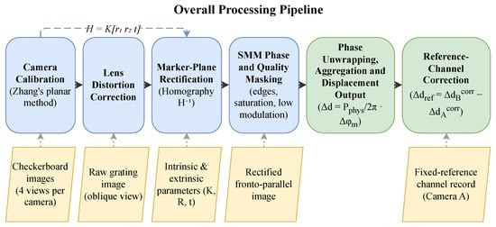
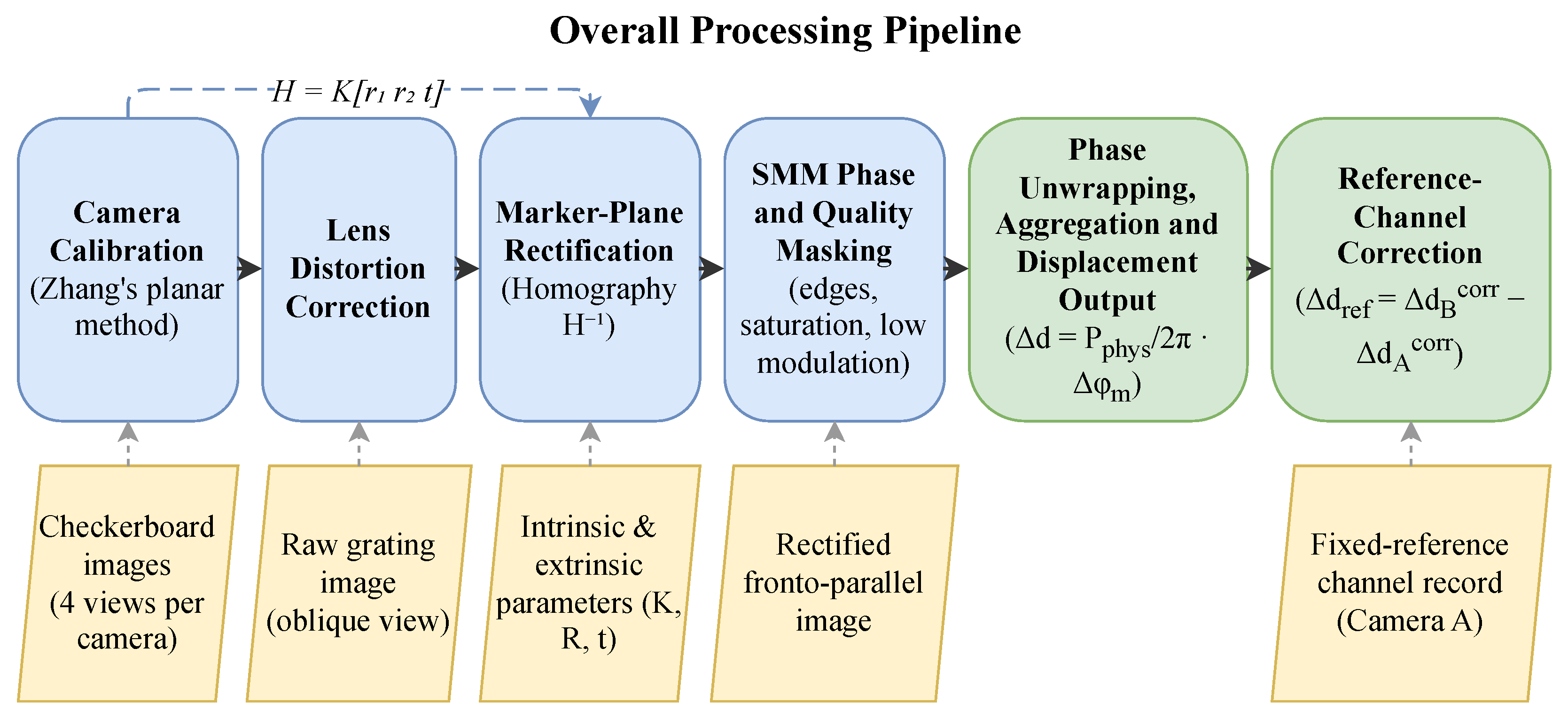
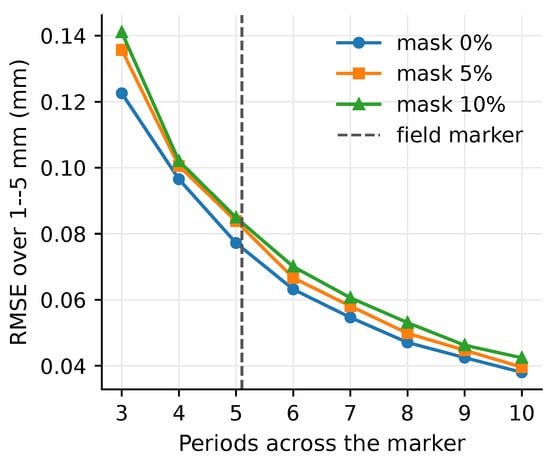
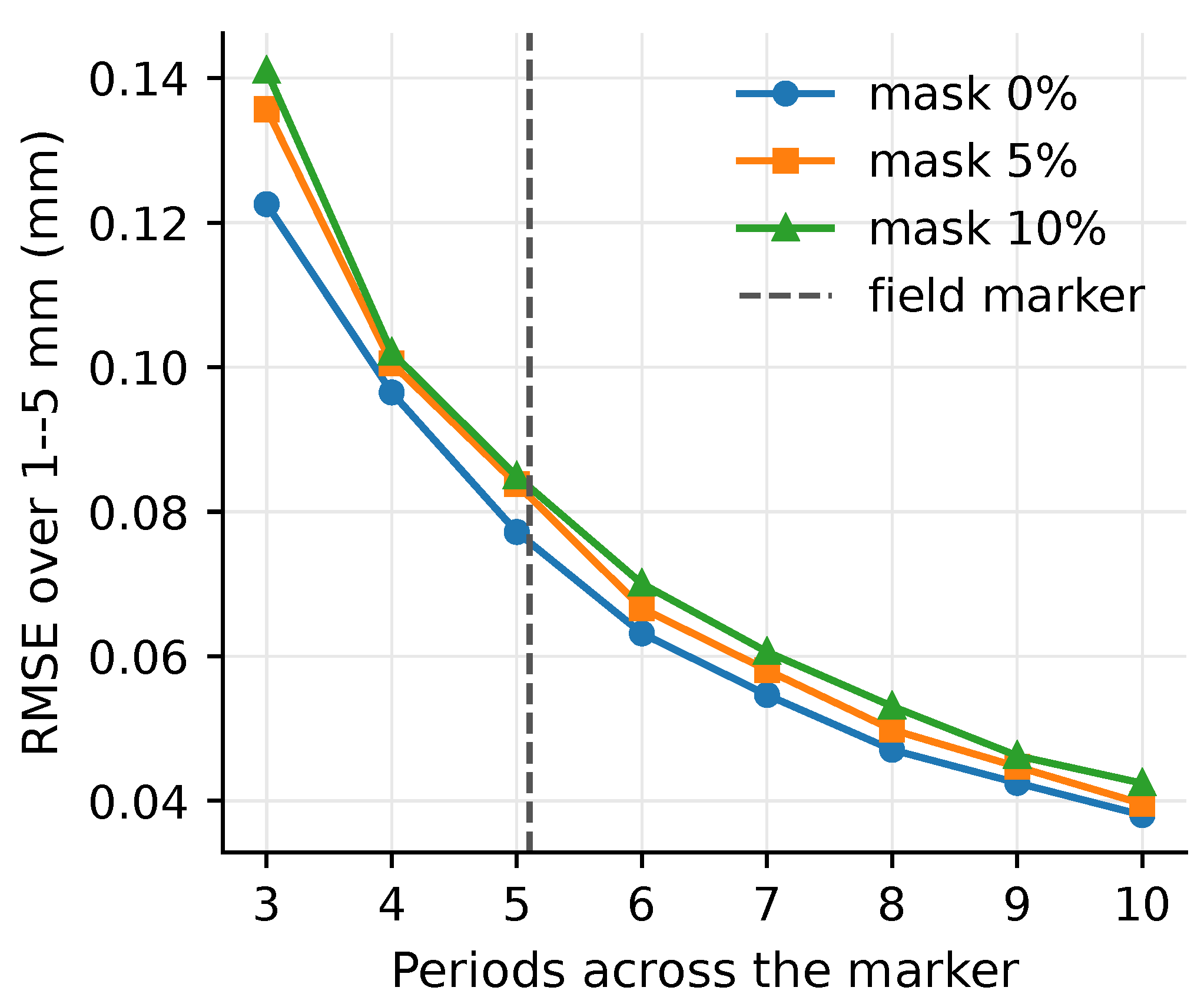
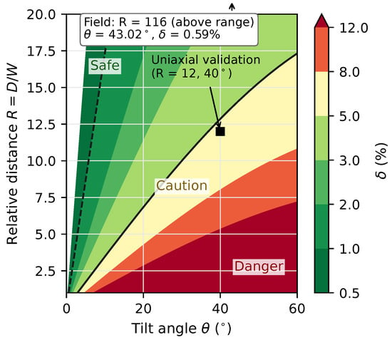
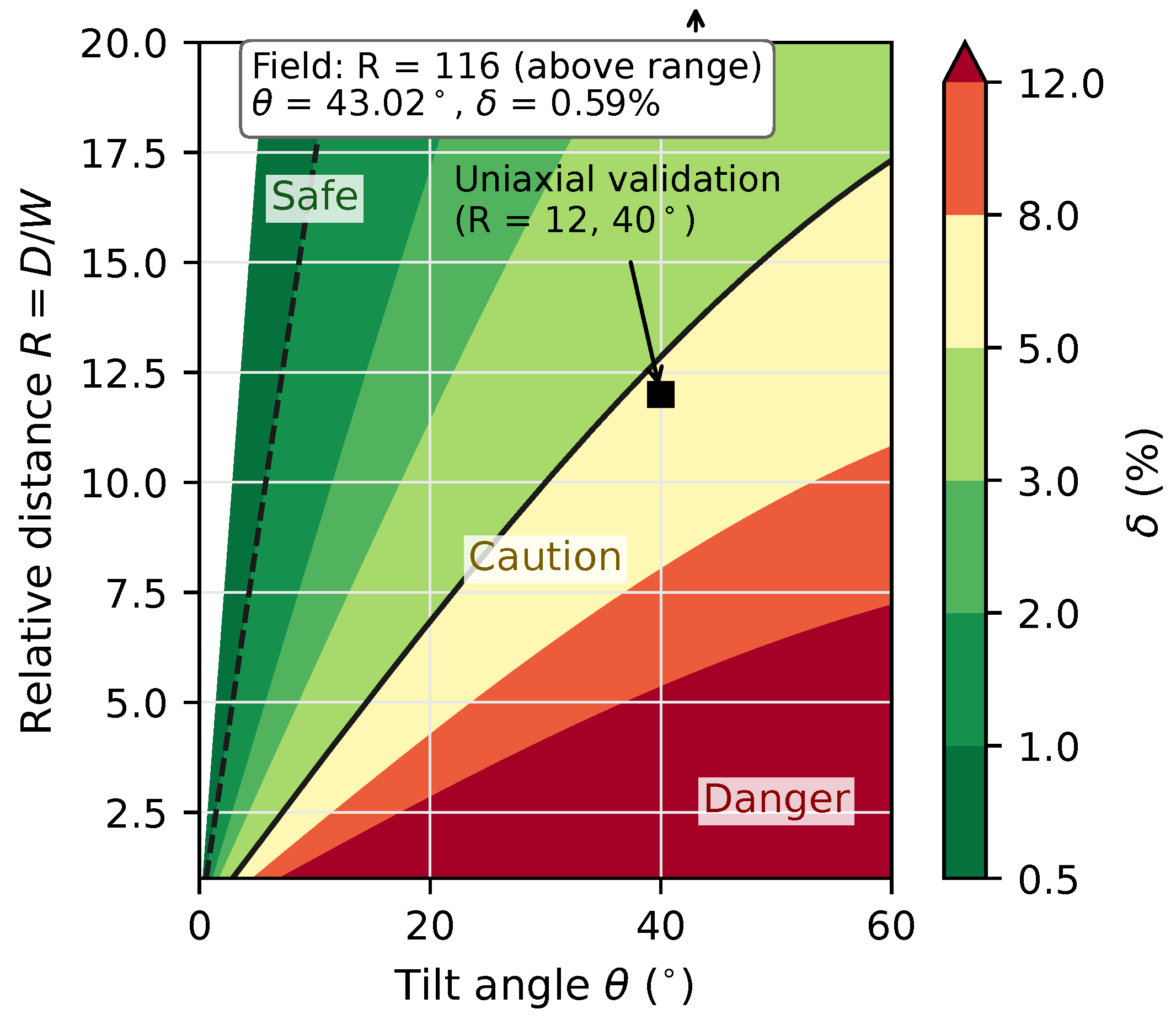
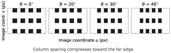
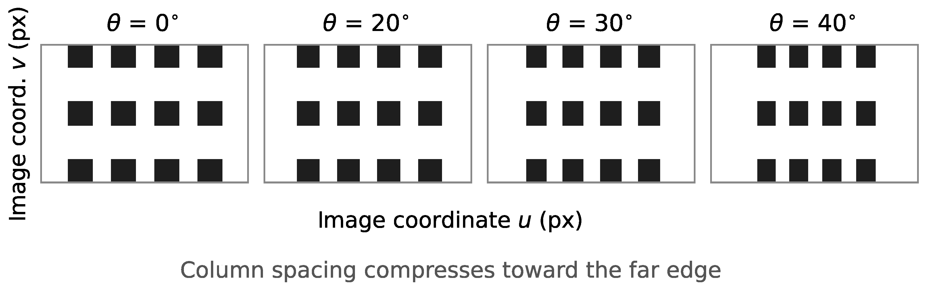
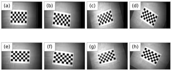
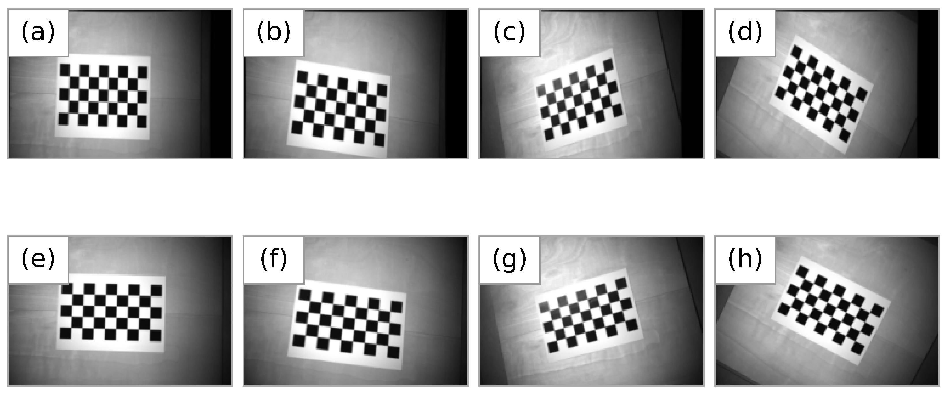
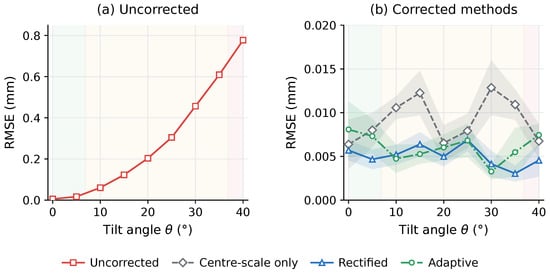
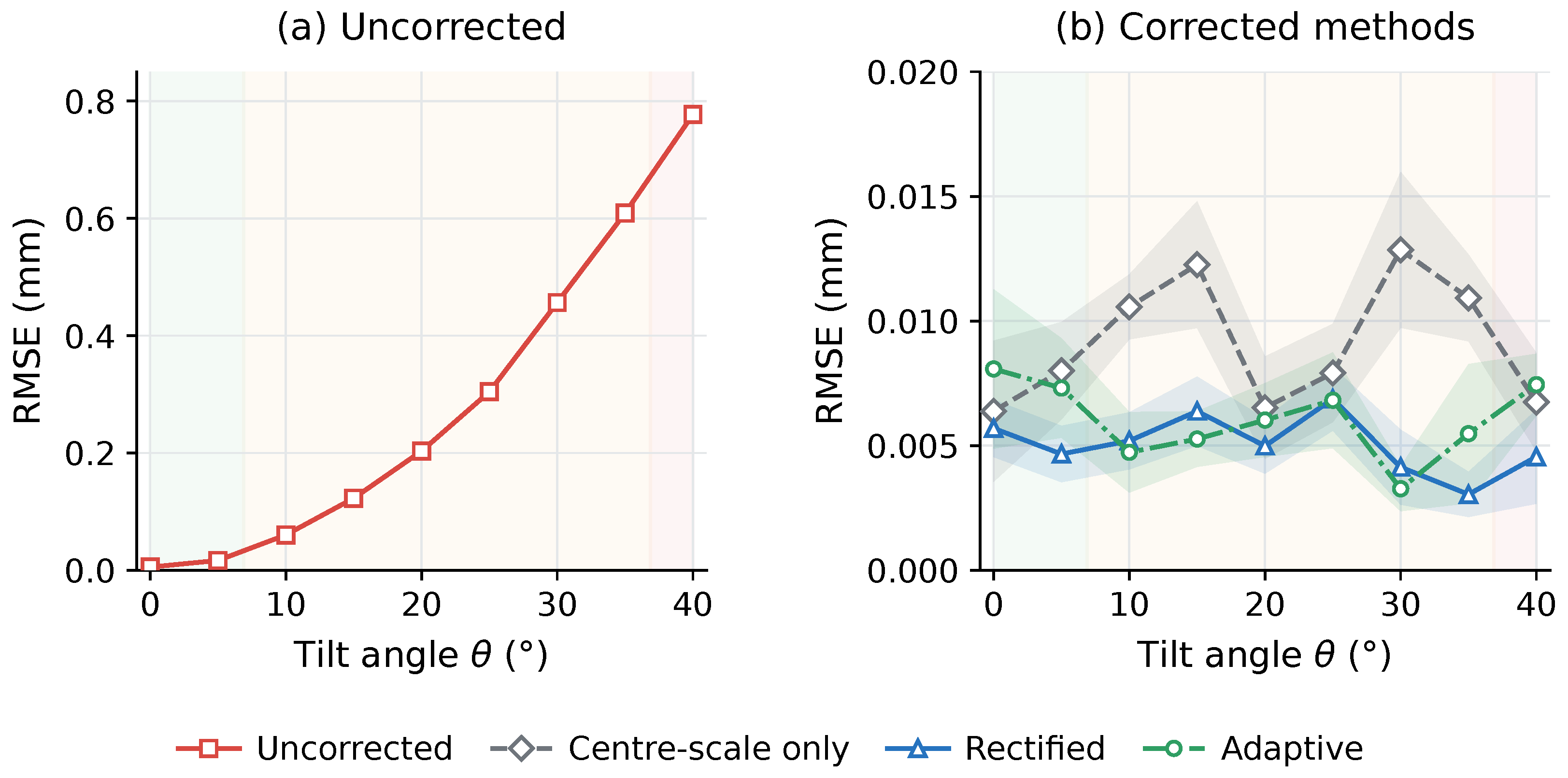
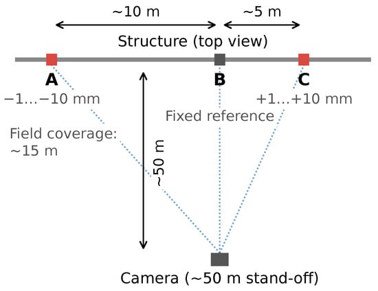
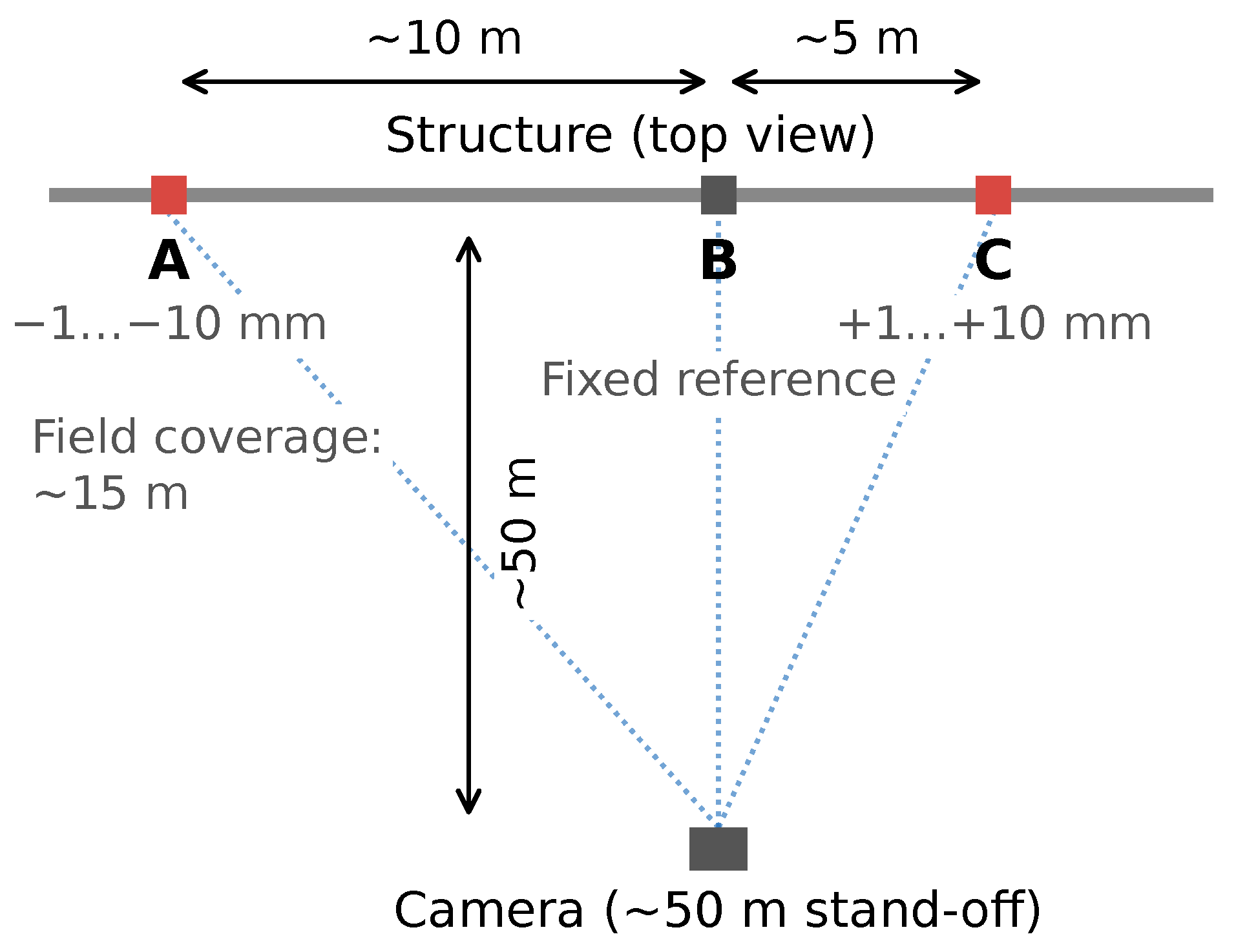
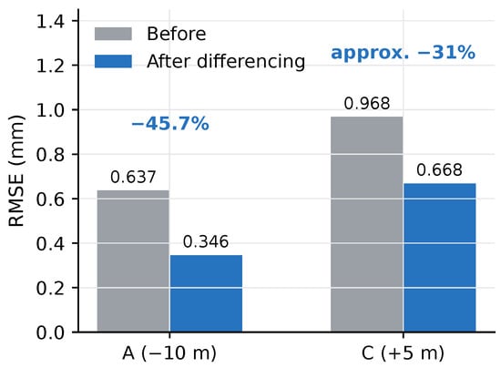
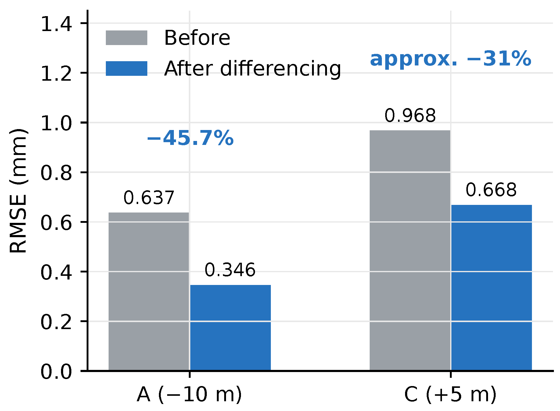
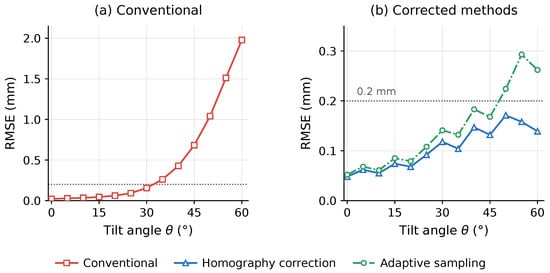
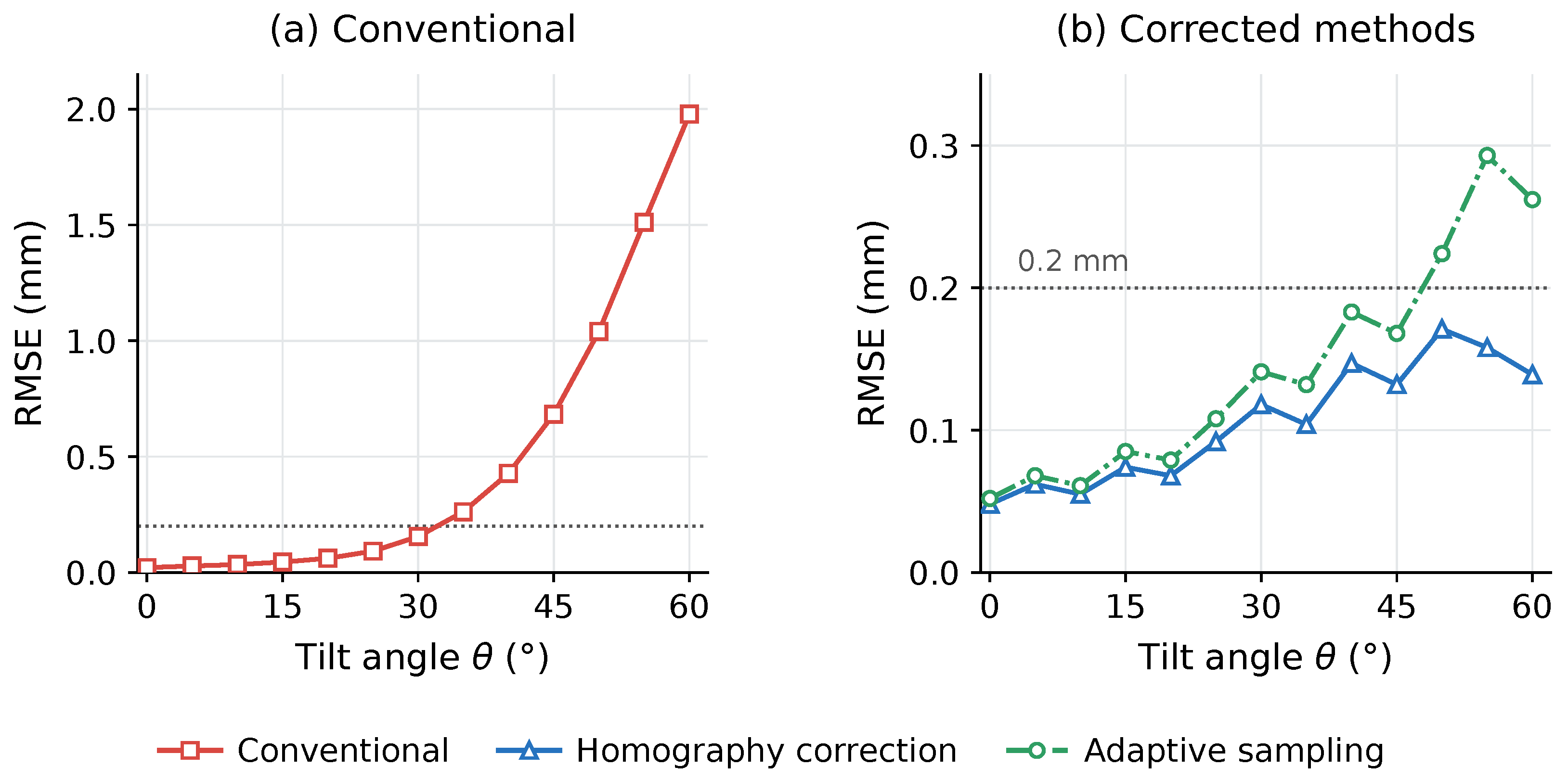
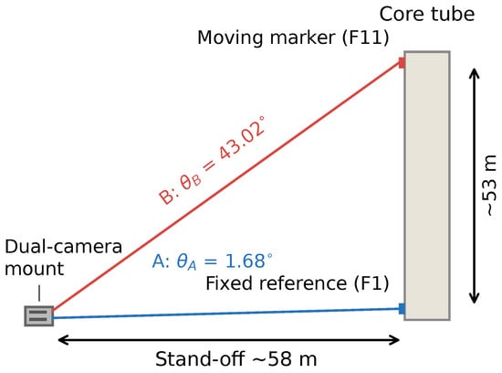
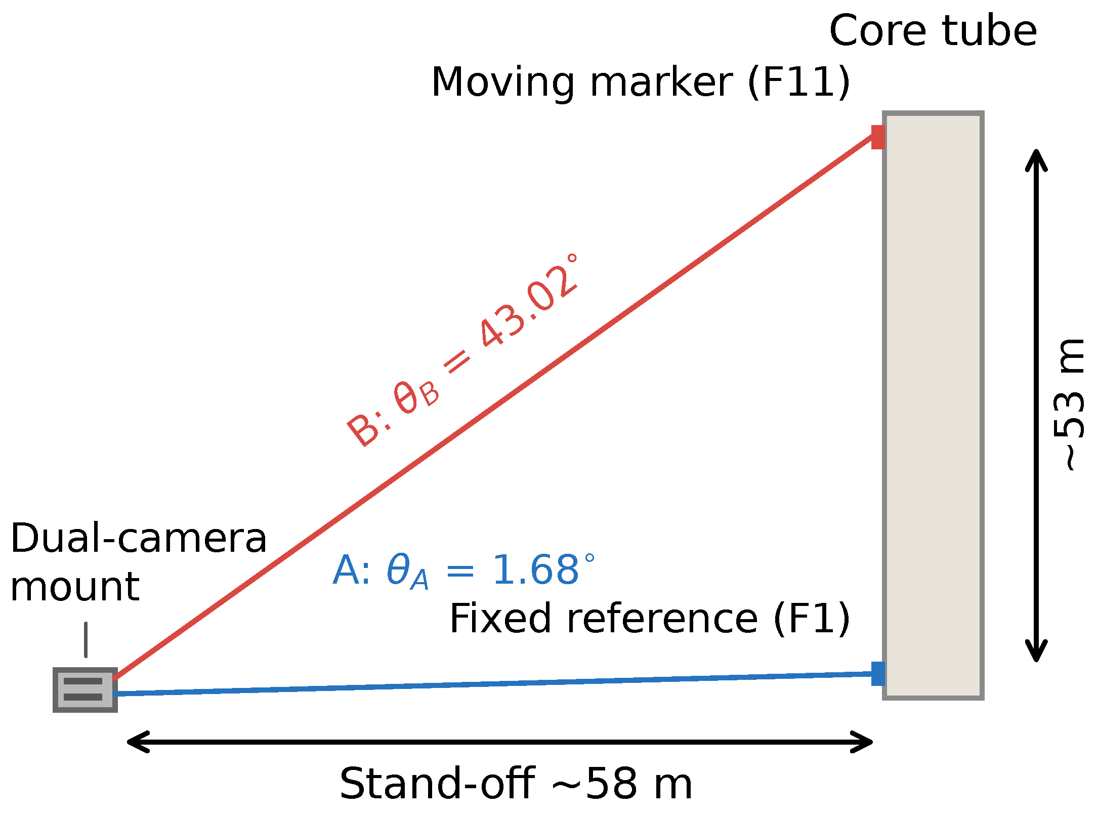
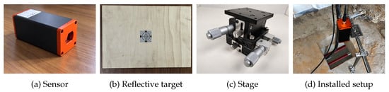
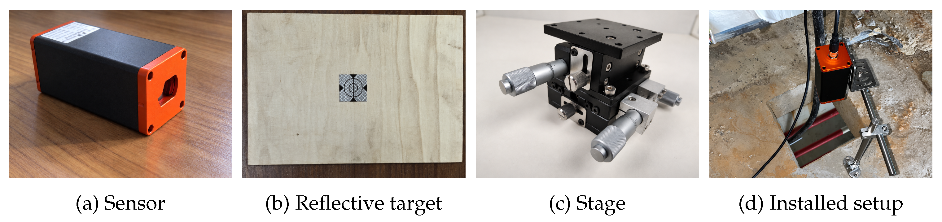
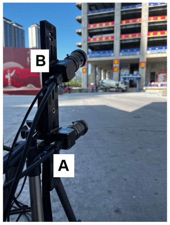
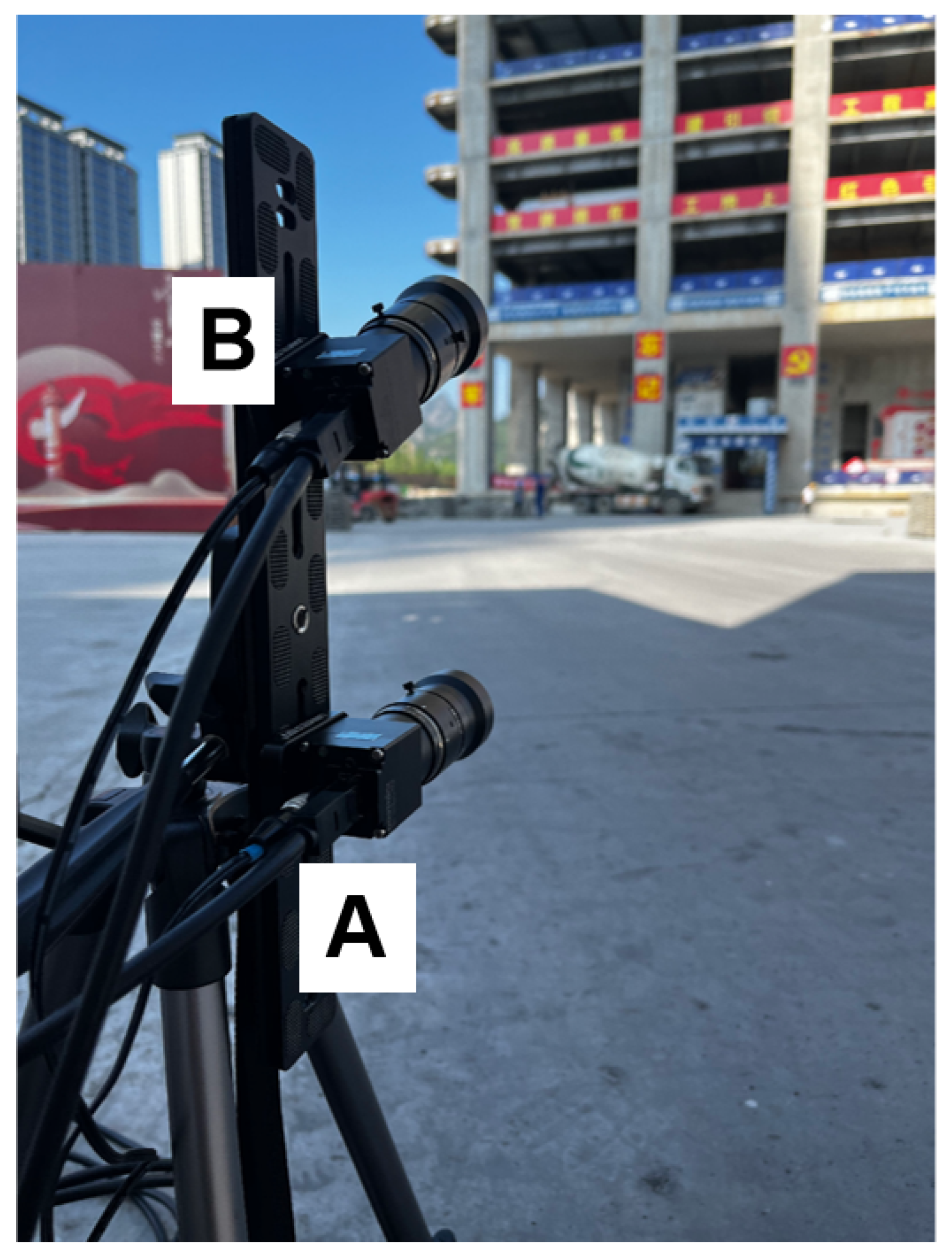
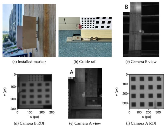
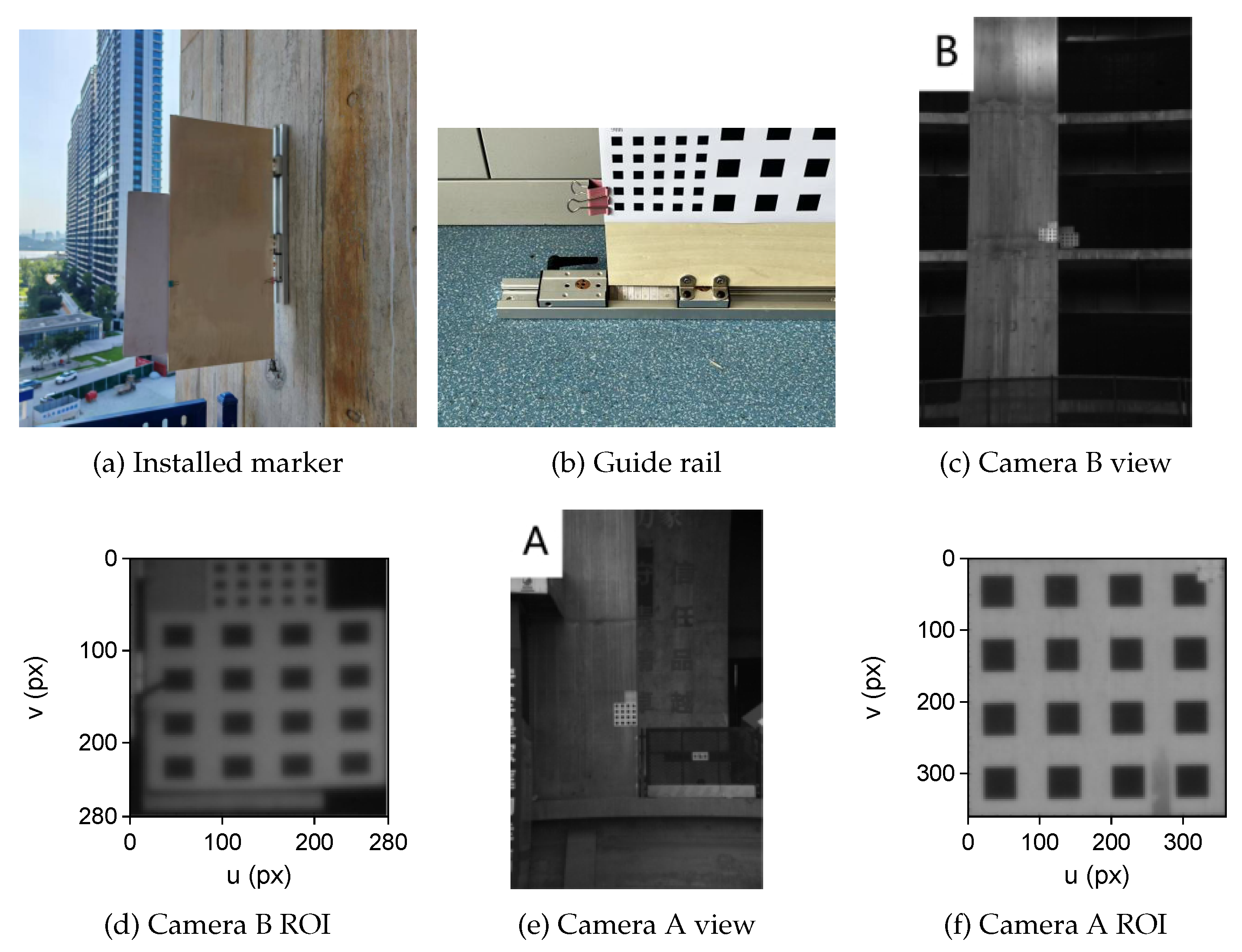
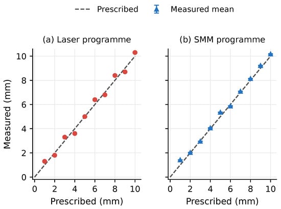
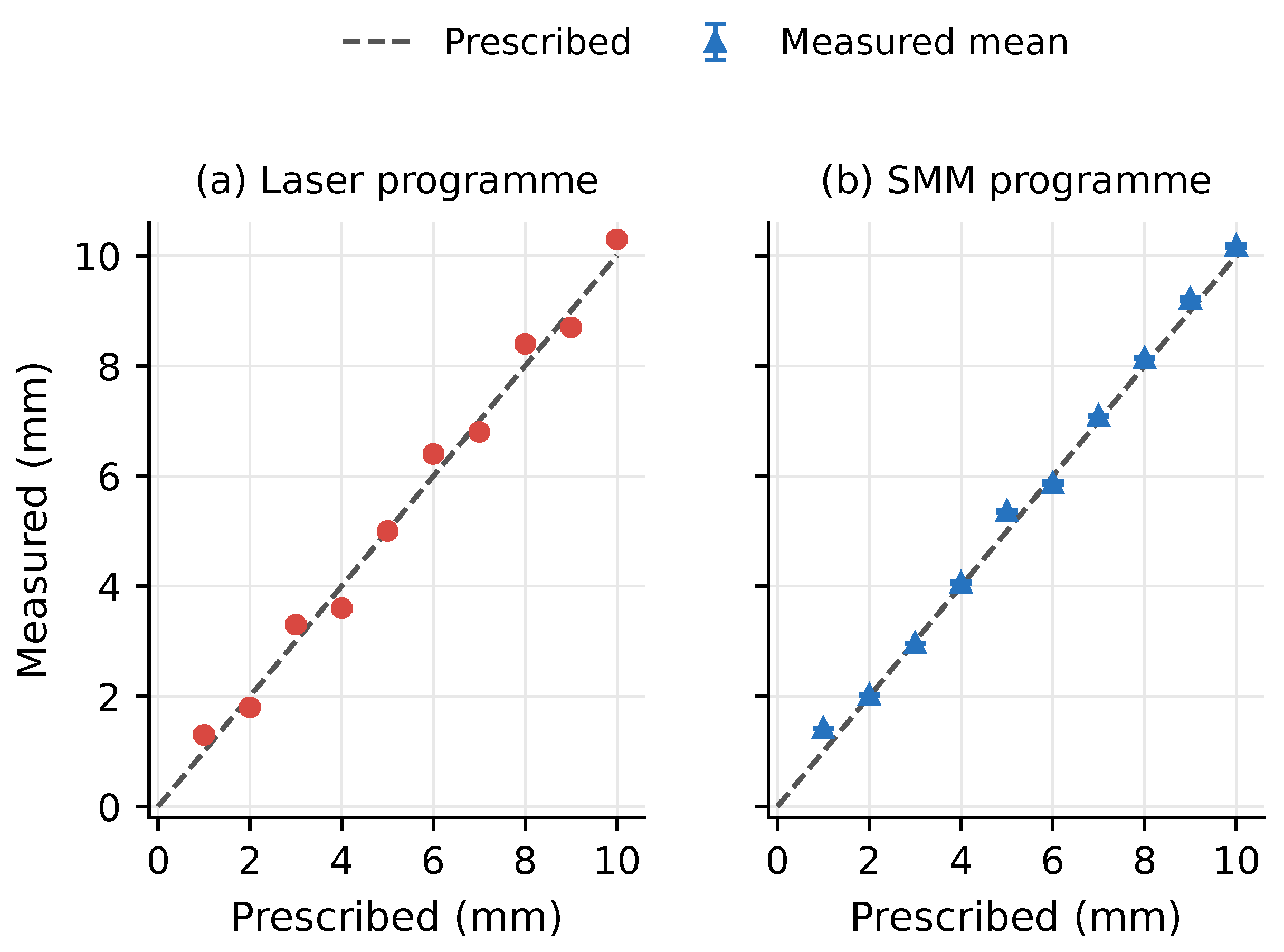
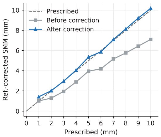
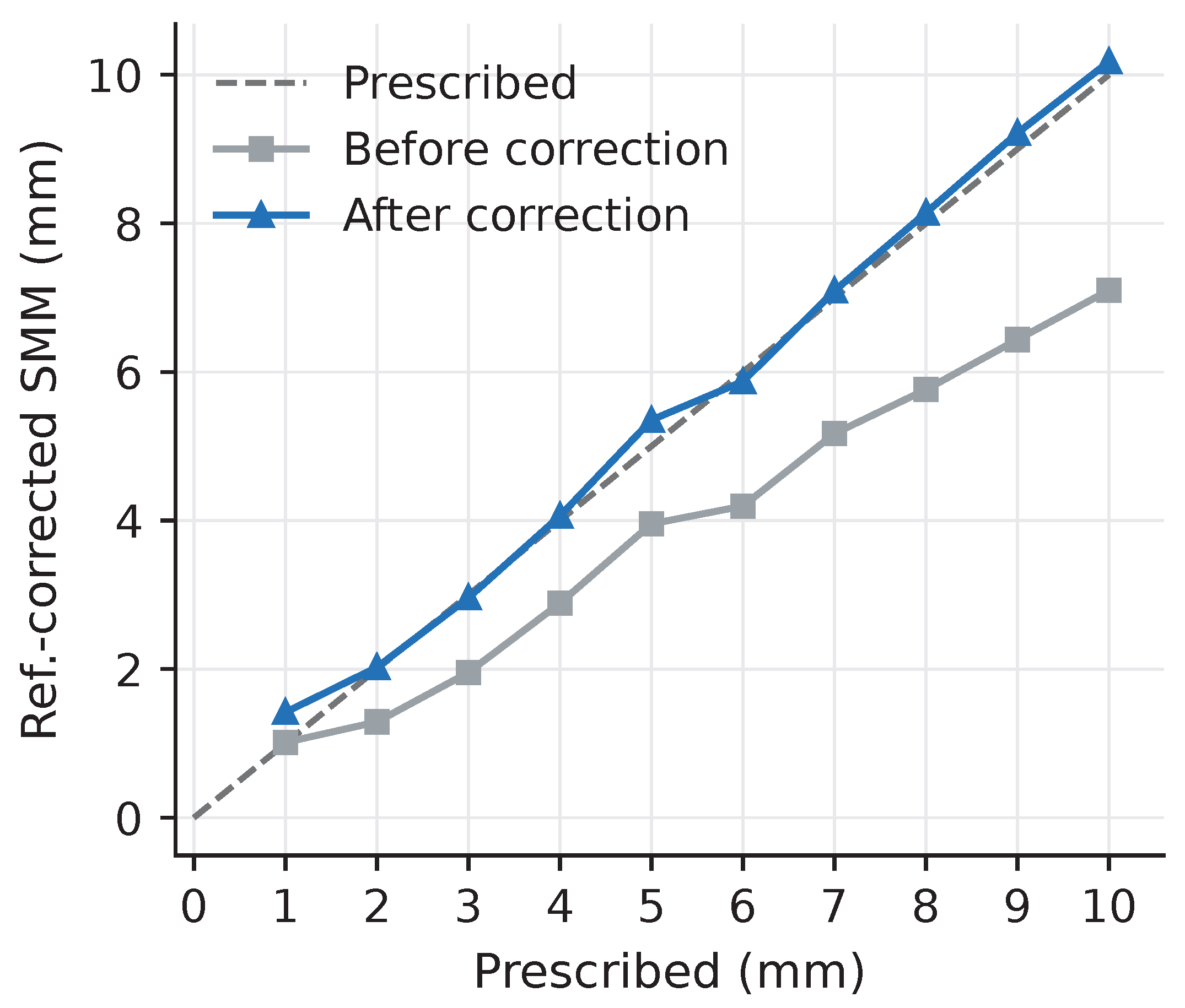

Disclaimer/Publisher’s Note: The statements, opinions and data contained in all publications are solely those of the individual author(s) and contributor(s) and not of MDPI and/or the editor(s). MDPI and/or the editor(s) disclaim responsibility for any injury to people or property resulting from any ideas, methods, instructions or products referred to in the content. |
© 2026 by the authors. Licensee MDPI, Basel, Switzerland. This article is an open access article distributed under the terms and conditions of the Creative Commons Attribution (CC BY) license.