Cable Damage Identification of Long-Span Cable-Stayed Bridges Using Spatial-Attention-Enhanced Multilayer Perceptron

Abstract

Stay cables are essential load-bearing elements of long-span cable-stayed bridges but are highly susceptible to degradation and fatigue. This study develops a deep learning framework for locating and quantifying stay cable damage. All training, validation, and independent test data in this study were generated by an OpenSees finite element model covering different cable damage locations and severities. A multilayer perceptron (MLP) classification model integrated with a spatial attention module (SAM) is constructed to achieve accurate localization of damaged stay cables. Based on this, a regression model with a similar architecture to the classification model is employed for damage quantification. In this identification procedure, SAM is adopted to enhance key spatial features, and MLP is used to separately train the Damage Location Identification Model (DLIM) and Damage Severity Identification Model (DSIM). After training, the identification accuracy of DLIM reaches 99.91%, and the identification reliability of DSIM reaches 99.95%. Under a signal-to-noise ratio (SNR) of 15 dB, the DLIM accuracy and DSIM reliability remain 94.76% and 97.33%. The framework provides a numerical case-study assessment of stay cable damage identification under the tested data protocol and Additive White Gaussian Noise (AWGN) condition.

1. Introduction

Stay cables are essential load-bearing elements in cable-stayed bridges, facilitating load transfer between the bridge deck and tower. These components, however, are susceptible to cyclic fatigue, environmental corrosion, and material aging, which degrade their mechanical properties [1]. With rising demands for the reliability of transportation infrastructure, pinpointing damaged cables and assessing their damage extent have become a central focus in structural health monitoring (SHM). This is crucial for developing preventive maintenance strategies and preventing catastrophic failures [2].

Early techniques for identifying damage in stay cables primarily relied on vibration-based detection methods. Zui et al. [3] determined cable tension by analyzing the natural frequency, combined with the cable’s mass per unit length and vibration length. While widely used in engineering, this method’s accuracy is heavily influenced by boundary conditions. To enhance accuracy, Casas [4] incorporated various vibration signals in the analysis of cable tension. Kim and Park [5] employed a frequency-based system identification approach, developing a finite element model that accounted for sag and bending stiffness, achieving an estimation error of less than 3%. Despite these advancements, most methods exhibit low sensitivity to early cable damage. Russell & Lardner [6] validated the theoretical predictions by comparing them with experimental results from a 1:10 scale model, confirming the relationship between frequency and tension in elastic cables. These studies have advanced the practical application of vibration theory in engineering. Nonetheless, sensor technology limitations impede spatial resolution and temporal consistency in data acquisition, necessitating manual data analysis and hindering real-time monitoring.

Advancements in sensor technology have ushered stay cable monitoring into an era of automation and distributed sensing. Innovations such as fiber-optic sensing, wireless sensor networks, and robotic detection have shifted the paradigm from point-based to distributed monitoring. Kamal and Mansoor [7] evaluated various cable tension estimation methods, concluding that real-time monitoring via wireless sensor networks effectively tracks tension changes. Cho et al. [8] developed an automated wireless tension estimation system, enabling synchronous monitoring of extensive stay cable groups through distributed sensor nodes. However, this system faces challenges with data transmission delays and electromagnetic interference. Li et al. [9] addressed the limitations of traditional corrosion detection methods by creating a mathematical model linking corrosion mass loss in prestressed anchor cables to axial fiber strain using axially distributed fiber-optic sensors. Despite effectively locating corrosion areas, this method requires integrated sensor installation during cable manufacturing, complicating its application in existing bridge renovations. The textile-embedded fiber-optic sensing system enables continuous strain monitoring over a 28 m range using optical frequency domain reflectometry, addressing the limited spatial coverage of traditional discrete sensors. Nevertheless, practical applications must balance monitoring accuracy with system cost [10]. While these technologies enhance the timeliness and spatial coverage of cable monitoring, their long-term stability and reliability in extreme environments require further validation. Guo and Zhu [11] identified significant variations in vibration energy distribution across different cable positions, necessitating refined sensor deployment strategies. Multi-sensor data fusion technology demonstrates significant potential, as evidenced by Diamanti and Soutis [12], who proposed a multi-physical field fusion method for monitoring aviation composites. By integrating fiber-optic and acoustic sensing data to develop a damage identification model, this approach effectively addresses the limitations of single-sensing technologies in identifying complex damages. This method holds promise for improving the detection of corrosion–fatigue-coupling damage in stay cables.

The integration of artificial intelligence (AI) technology offers a novel data-driven approach for damage detection in health monitoring systems. Hao and Xia [13] employed a real-coded genetic algorithm (GA) for structural damage identification, leveraging GA’s global search capability to address nonlinear problems, though with low computational efficiency. Lee et al. [14] developed a damage identification system using neural networks, effectively mitigating modeling errors in finite element models (FEMs), but it demands extensive high-quality modal data, incurring significant data acquisition costs. To tackle pervasive uncertainties in structural monitoring, Bakhary et al. [15] introduced an artificial neural network (ANN) model incorporating statistical methods, enhancing the reliability of identification results by systematically addressing dual uncertainties; however, it struggles with small-sample data adaptability. Chandrashekhar and Ganguli [16] applied fuzzy logic to reduce uncertainties from geometric parameters and measurement errors, yet its accuracy falters in multi-damage scenarios. In 2013, Li et al. [17] proposed a symbolic differential evolution (DE) strategy, which accelerates parameter identification, but the symbolic process risks feature information loss, and its efficacy diminishes in noisy environments. Ding et al. [18] enhanced the artificial bee colony algorithm (ABC), which offers superior global search and anti-noise capabilities, though it incurs high computational costs. Padil et al. [19] demonstrated the efficacy of ANN for damage identification under uncertainty, yet it remains constrained by reliance on feature engineering. Pathirage et al. [20] introduced a damage identification framework using autoencoders, which autonomously extracts high-dimensional nonlinear features through unsupervised learning, reducing manual feature design costs. However, its effectiveness is contingent on extensive labeled data.

In data-driven damage identification, advancements aim to enhance anti-interference and minimize data dependency. These methods are extensively applied in structural health monitoring [21,22,23,24,25,26,27]. Recent studies further address data scarcity and non-stationarity through incremental ensemble learning [28], improve the interpretability and feature selection of data-driven damage identification [29], and combine transfer learning with residual attention for small-sample, noise-affected structural damage classification [30]. Yet, for long-span cable-stayed bridges, three limitations remain: monitoring coverage is often limited by cost and accessibility; the large number and near-symmetrical arrangement of stay cables can produce confusing response patterns for similar cables; and measurement noise and model uncertainty can obscure damage-related features. In cable-specific damage identification, Ren et al. [31] used bridge-deck strain measurements with support vector machines to identify damaged cables and estimate severity, while related simulation and machine-learning studies based on moving-vehicle vibration responses and multi-load response prediction address different dynamic-response settings [32,33]. Recent monitoring studies also show complementary strategies: physics-informed baselines can account for environmental effects in displacement monitoring, while extreme-function methods can detect deviations using experimental bridge data [34,35]. These studies address environmental baseline or experimental damage detection, rather than the present stay cable localization task, and therefore help define the remaining transfer and field-validation gap.

This study proposes an efficient deep learning framework that integrates a multilayer perceptron (MLP) with a spatial attention module to detect and assess damage in stay cables. The model is trained using a dataset generated by the finite element method and can capture complex nonlinear relationships between structural response features and damage states. The spatial attention module processes the ordered feature-index information of the sensor data and emphasizes spatial features relevant to the current damage scenario. The MLP then performs multilayer nonlinear transformations for classification and regression tasks. Two independently trained deep learning models are developed for these tasks: the Damage Location Identification Model (DLIM) and the Damage Severity Identification Model (DSIM). Finally, the performance of the proposed framework is assessed through a numerical case study using FEM-generated data.

2. Materials and Methods

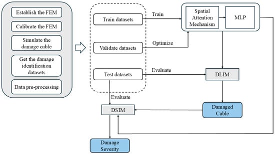
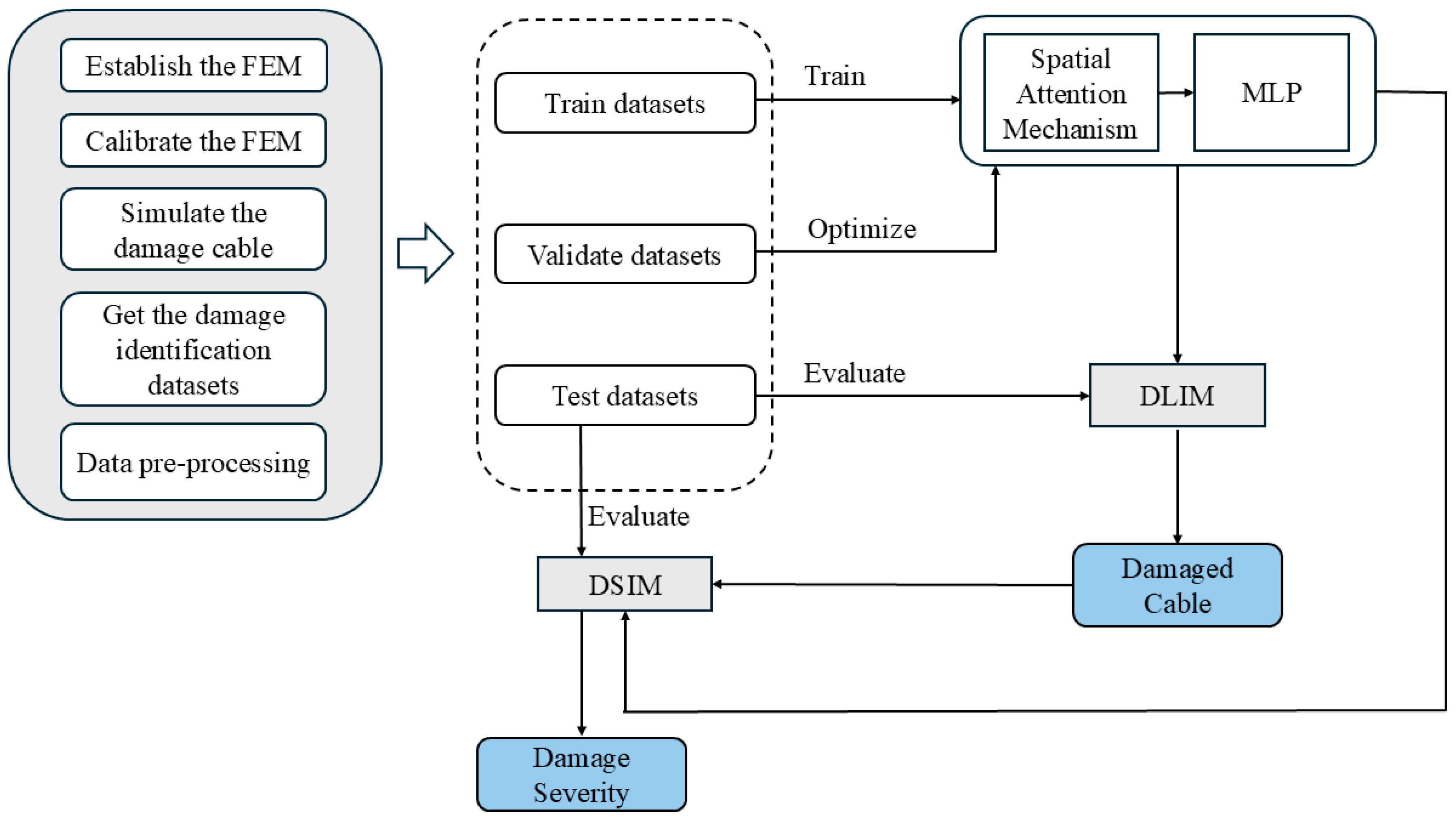
Figure 1 illustrates the methodological framework employed in this study. Initially, a finite element model was developed via OpenSees (version 3.3.0; Pacific Earthquake Engineering Research Center, Berkeley, CA, USA). This model was further calibrated to simulate cable damage and utilized to compute the deflection response of the girder, thereby constructing the initial dataset. Subsequently, the initial dataset is preprocessed and divided into a training set and a validation set at a ratio of 8:2. The training set was first processed using a spatial attention module to generate attention weights for each feature; these weights were then incorporated into the training process of a multilayer perceptron (MLP). The MLP was further validated and iteratively optimized using the validation set to enhance its predictive stability. On this basis, the Damage Location Identification Model (DLIM) is constructed, and precise localization of damaged stay cables is achieved through model training. Concurrently, the Damage Severity Identification Model (DSIM) is independently trained to quantify the damage severity of the stay cables. Finally, an independent test set is used to evaluate the performance of both DLIM and DSIM. Detailed specifications of the aforementioned models are provided in Section 2.1, Section 2.2 and Section 2.3, whereas the methodology for dataset construction is elaborated in Section 3.

Figure 1. Framework of the SAM-MLP model for cable damage identification.

2.1. Deep Learning Model Combining Spatial Attention Module and Multilayer Perceptron (SAM-MLP Model)

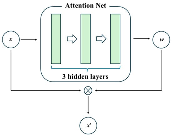
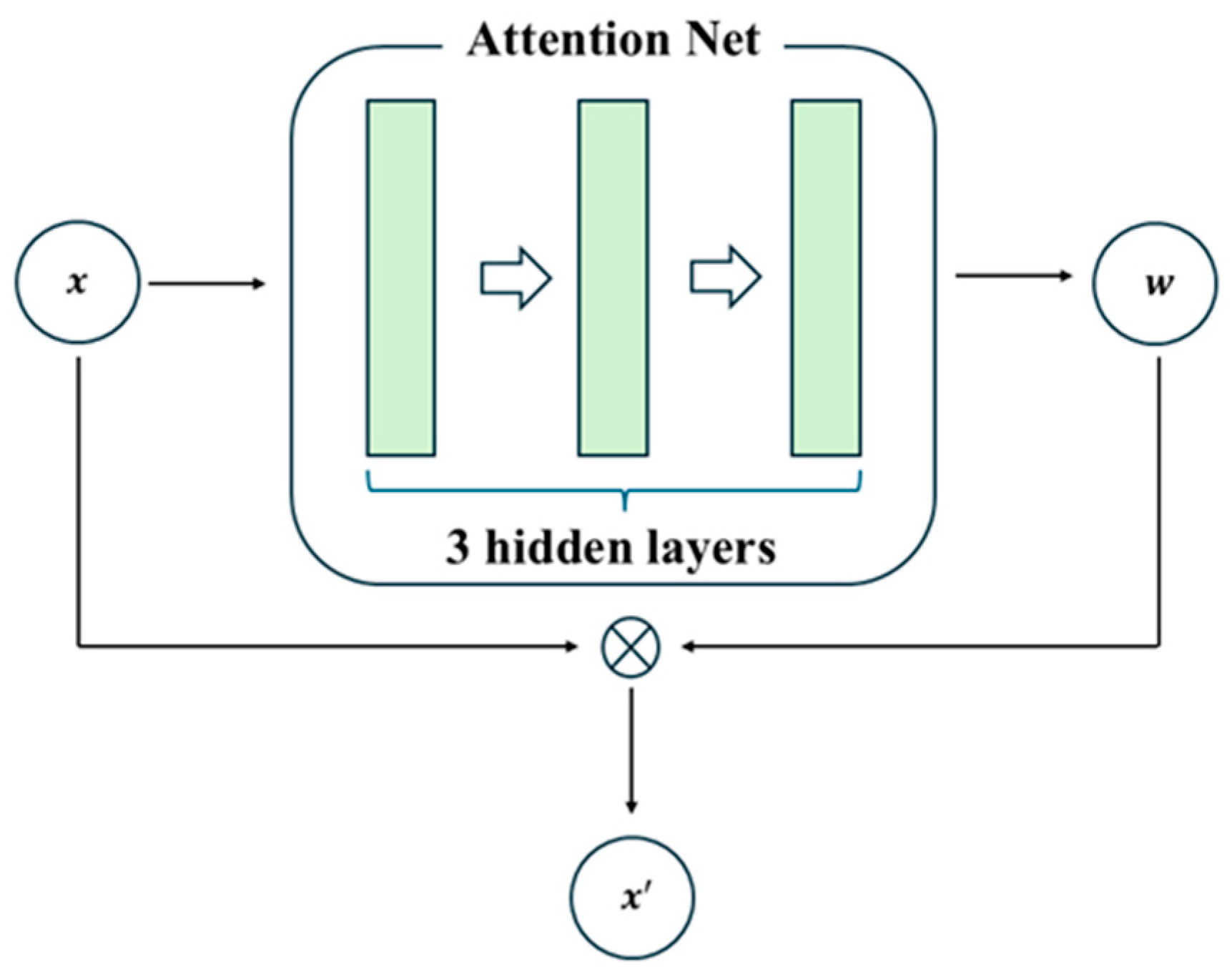
The spatial attention module (SAM) is implemented here as a feature-index weighting block. The term “spatial” refers to the ordered indices of the 136 cable-anchor features; physical coordinates, anchor distances, and an adjacency matrix are not supplied to the module. SAM therefore learns sample-dependent feature weights rather than an explicit physical-space or causal representation.

The spatial attention module operates through weight calculation and feature weighting [36], as shown in Figure 2. In the implementation, for an input vector x in R¹³⁶, the attention network follows Linear(136,128), LayerNorm(128), ReLU, Linear(128,64), ReLU, Linear(64,136), and Softmax(dim = 1). In compact form,

a(x) = Softmax(W3 ReLU(W2 ReLU(LN(W1x + b1) + b2)) + b3),

where W1, W2, and W3 map 136→128, 128→64, and 64→136, respectively; the weighted feature vector is x_w = x⊙a(x), where ⊙ denotes element-wise multiplication. The weighted vector is then passed to the MLP. Because no explicit coordinates, distances, or adjacency matrix are provided, the learned weights are feature-index weights. They indicate which ordered inputs receive greater model emphasis for a given sample.

Figure 2. Operating mechanism of the spatial attention module.

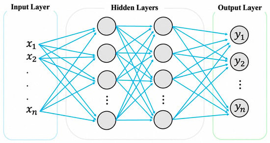
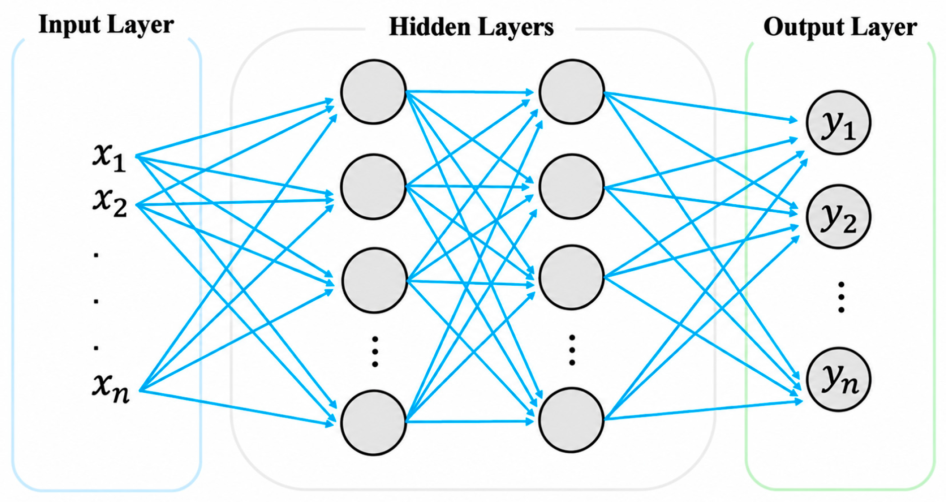
The multilayer perceptron (MLP), a fundamental branch of artificial neural networks (ANNs), represents the quintessential fully connected network architecture in deep learning [37,38]. It employs supervised training via backpropagation [39]. Essentially, MLP simulates “human neuron signal transmission,” enabling nonlinear feature extraction and task mapping through the coordinated computation across multiple neuron layers. Its structure adheres to a “layered progression” comprising three components: the input layer, hidden layer, and output layer. Each layer contains several neurons, and neurons in adjacent layers are fully connected, meaning every neuron in one layer connects to all neurons in the next, without skipped or local connections [40], as depicted in Figure 3. The input layer serves as the interface between the MLP and external data, receiving N features (x₁, x₂, x₃, …, x_n). Following the hidden layer’s computation, the neural network’s predicted response emerges at the output layer (y₁, y₂, y₃, …, y_n). The number of neurons per layer and the total number of layers are hyperparameters that can be optimized to enhance model efficiency.

Figure 3. MLP with two hidden layers.

Neurons in adjacent layers communicate via activation functions. The output of a single neuron can be represented by Equation (1).

$$y_i=\sigma (\sum _i{w}_i^{\mathit{MLP}}{x}_i+b_i)$$

(1)

In this context, σ is the activation function, while x_i represents the input value, and w_i and b_i are the weight and bias, respectively. Unlike the sigmoid and hyperbolic tangent functions, the rectified linear unit (ReLU) effectively mitigates the vanishing gradient issue, making it a preferred choice. ReLU is currently among the most prevalent activation functions [41]. The ReLU function is defined by Equation (2).

ReLU(x) = max(x,0)

(2)

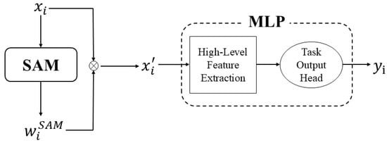
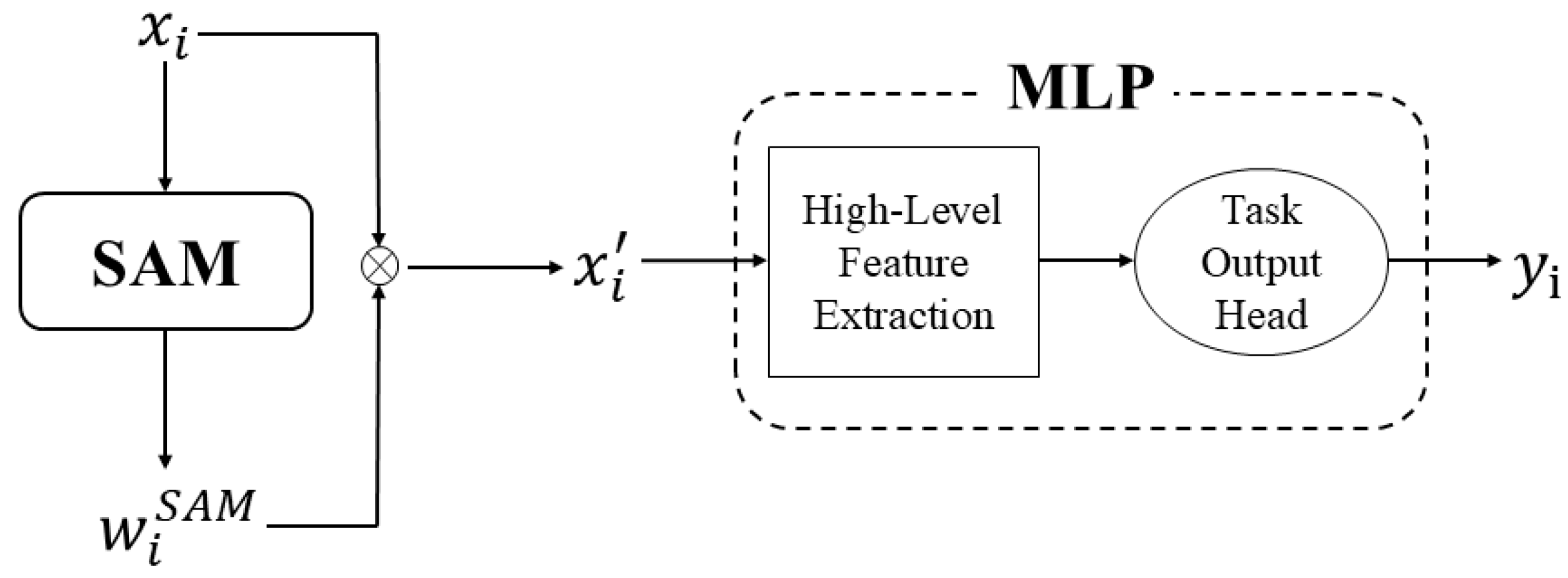
The SAM-MLP model combines feature-index reweighting with an MLP. The attention block assigns a sample-dependent normalized weight to each ordered input feature, and the weighted vector is then processed by the fully connected layers to produce the location or severity output of the corresponding single-task model. No explicit physical coordinate or causal adjacency is encoded by this operation. As illustrated in Figure 4, the numerical comparison in this study shows that SAM-MLP provides the most balanced cross-SNR performance under the stated FEM-generated dataset and AWGN protocol [42].

Figure 4. Schematic diagram of the SAM-MLP model structure.

Here, x_i represents the input features, $w_i^{\mathit{SAM}}$ denotes the attention weights, $x_i^{\prime }$ stands for the weighted features, and y_i is the model’s prediction result.

2.2. Damage Location Identification Model (DLIM)

Identifying the damaged cable constitutes a single-task classification problem. The current implementation combines a feature-index attention module with an MLP and predicts one of 136 cable location classes. It uses weighted cross-entropy as the loss function [43]; the calculation method is detailed in Equation (3). DLIM and DSIM are trained independently and do not share a multi-task output head.

$$L_{\mathit{CE}}=-{\displaystyle \frac{1}{N}}{\sum }_{i=1}^N{\sum }_{c=1}^C{w}_c{y}_{i,c}\mathit{log}\left(p_{i,c}\right)$$

(3)

Here, N denotes the number of batch samples, and C represents the number of categories, specifically the 136 single-side cables of the long-span cable-stayed bridge under study. w_c is the weight for the c_th category. y_i,c is the one-hot label of the i_th sample, where y_i,c = 1 indicates that it belongs to the c_th class, and otherwise it is 0. p_i,c is the predicted probability that the i_th sample belongs to the c_th category. The model utilizes the AdamW optimizer [44] and a cosine annealing learning rate scheduler. The dataset, derived from a finite element model, is detailed in Section 3. Model performance is assessed using prediction accuracy and Top-k accuracy, with prediction accuracy calculated as shown in Equation (4).

$$\mathit{Acc}={\sum }_{i=1}^{N_e}{\displaystyle \frac{\mathbb{1}\left(r_{\mathit{pred},i}=r_{\mathit{true},i}\right)}{N_e}}$$

(4)

Among them, N_e is the total number of evaluation samples, r_pred,i is the predicted value of the i_th sample, and r_true,i is the true value of the i_th sample. $\mathbb{1}(·)$ is an indicator function (taking the value of 1 when the condition is true and 0 otherwise).

The equation for calculating the Top-k accuracy is shown in Equation (5).

$$\mathit{Top}-k\mathit{Acc}={\sum }_{i=1}^{N_e}{\displaystyle \frac{\mathbb{1}\left(t_{\mathit{true},i}\in {\mathit{Top}}_k\left(p_{\mathit{pred},i}\right)\right)}{N_e}}$$

(5)

Here, t_true,i represents the true cable index of the i_th sample, and p_pred,i is the 136-dimensional predicted probability vector of the i_th sample. Top_k(p_pred,i) denotes the set of indices corresponding to the largest Top-k probabilities in p_pred,i.

DLIM uses hidden dimensions [256,128,64], dropout of 0.3, batch size of 128, 80 maximum epochs, learning rate of 3 × 10⁻³, AdamW weight decay of 5 × 10⁻⁵, patience of 15, and seed 42. The cosine scheduler uses T_max = epochs and eta_min = 10⁻⁵. The class weight for class c is calculated from the training-label count n_c as w_c = (1 − s)/(n_c + 10⁻⁶) + s/C with smoothing s = 0.1 and C = 136, followed by normalization to mean of one. DSIM uses a separate regression model with hidden dimensions [128,64], dropout of 0.4, batch size of 128, 100 maximum epochs, learning rate of 10⁻³, AdamW weight decay of 10⁻⁴, patience of 15, and the same cosine-scheduler form.

2.3. Damage Severity Identification Model (DSIM)

For stay cables, the Damage Identification Index’s absolute value rises with damage severity, as detailed in Section 3.3. Consequently, determining the damage severity in cables is treated as a regression problem. The damage identification model employs the Mean Squared Error (MSE) as its loss function [45], with the calculation outlined in Equation (6).

$$L_{\mathit{MSE}}={\displaystyle \frac{1}{N}}{\sum }_{I=1}^N{\left({\widehat{y}}_i-y_i\right)}^2$$

(6)

N denotes the number of samples per batch, with ${\widehat{y}}_i$ and y_i representing the predicted and true damage levels of the i_th sample, respectively. The model utilizes the AdamW optimizer alongside a cosine annealing learning rate scheduler. The dataset mirrors that of the DLIM. Model performance is assessed via mean absolute error (MAE), Root Mean Squared Error (RMSE), coefficient of determination (R²), uncertainty interval U95, and reliability [43]. The calculation methods for these metrics are detailed in Equations (7)–(11).

$$\mathit{MAE}={\displaystyle \frac{1}{N}}{\sum }_{I=1}^N\left|{y_i^{\mathit{ture}}-y}_i^{\mathit{pred}}\right|$$

(7)

$$\mathit{RMSE}=\sqrt{{\displaystyle \frac{1}{N}}{\sum }_{I=1}^N{\left(y_i^{\mathit{pred}}-y_i^{\mathit{ture}}\right)}^2}$$

(8)

$$R^2=1-{\displaystyle \frac{{\sum }_{i=1}^n{\left(y_i^{\mathit{ture}}-y_i^{\mathit{pred}}\right)}^2}{{\sum }_{i=1}^n{\left(y_i^{\mathit{ture}}-{\overline{y}}_i^{\mathit{true}}\right)}^2}}$$

(9)

$$U95={\displaystyle \frac{1.96}{N}}\sqrt{{\sum }_{i=1}^N{(y_i^{\mathit{ture}}-{\overline{y}}_i^{\mathit{ture}})}^2+{\sum }_{i=1}^N{(y_i^{\mathit{ture}}-y_i^{\mathit{pred}})}^2}$$

(10)

$$\mathit{Reliability}=({\displaystyle \frac{100\%}{N}}){\sum }_{i=1}^N{k}_i$$

(11)

Among them, $y_i^{\mathit{pred}}$ is the predicted value of the damage severity of the i_th sample, $y_i^{\mathit{ture}}$ is the true value of the damage severity of the i_th sample, ${\overline{y}}_i^{\mathit{true}}$ is the mean value of the true values of the damage severity of the i_th sample, N is the number of samples, and k_i is calculated in two steps. The first step is to calculate the relative average error (RAE), as shown in Equation (12).

$${\mathit{RAE}}_i=\left|{\displaystyle \frac{(y_i^{\mathit{ture}}-y_i^{\mathit{pred}})}{y_i^{\mathit{ture}}}}\right|$$

(12)

When RAE_i ≤ Δ, k_i = 1; otherwise, k_i = 0. Here, Δ is set to 0.05.

3. Dataset Development

3.1. Finite Element Modeling

The project this study relies on is the Sutong Yangtze River Highway Bridge, a long-span cable-stayed bridge in China. The bridge has a total length of 32.4 km, and the main bridge adopts a span arrangement of 100 m + 100 m + 300 m + 1088 m + 300 m + 100 m + 100 m. The bridge uses a double-tower, double-cable-plane steel box girder cable-stayed bridge structure, with a total of 272 parallel wire cable-stayed cables. The cables use 7 mm high-strength galvanized parallel steel wires, and the longest stay cable is 576.193 m.

The finite element model was established using OpenSees, an open-source software framework dedicated to earthquake and structural engineering simulations. This software offers a wide range of material models, structural elements, and analysis methods, meeting various requirements from linear analysis to nonlinear time-history analysis.

This study uses a mixed linear and nonlinear formulation. The main girder, auxiliary piers, and upper or transition segments of the towers are represented by elasticBeamColumn elements with linear elastic constitutive relations. The stay cables are represented by truss elements with Steel02 bilinear kinematic hardening and prescribed initial stresses, so their axial constitutive response is nonlinear. The lower-tower shafts are represented by dispBeamColumn elements with fiber sections composed of Concrete01 and Steel01 fibers, allowing concrete cracking and crushing and reinforcement yielding to be represented. ZeroLength elements with Steel01 are used for bearing and limiting components, and equalDOF constraints impose the prescribed tower–girder and pier–girder kinematic couplings. Rayleigh damping with a target damping ratio of 0.03 is introduced for the transient analysis. Therefore, the linear description applies to the explicitly elastic beam–column components, whereas nonlinear constitutive behavior is retained for the stay cables, lower-tower fiber sections, and bearing and limiting components. These choices define the response features used for damage identification: the elastic beam–column components establish the baseline load path, nonlinear cable and lower-tower sections allow stiffness-dependent redistribution, the equalDOF and ZeroLength representations impose the modeled support and restraint path, and the 3% Rayleigh damping mainly affects transient peak responses rather than the converged gravity state.

To provide quantitative evidence for the finite element model used to generate the learning data, the model-updating results reported in Ref. [32] are summarized here. A One-At-a-Time sensitivity analysis evaluated eight parameters, including the equivalent densities and elastic moduli of the main span, side spans, and tower, together with the damping ratio and initial cable force. The four parameters with the highest sensitivity coefficients were the tower-equivalent density (0.2470), tower elastic modulus (0.0881), main span-equivalent density (0.0636), and main span elastic modulus (0.0253). After Bayesian-optimization updating, the average absolute percentage error of the seven target modal frequencies was 0.99%, and the MAC values between the initial and updated mode shapes ranged from 0.9037 to 0.9999. These results support the modal fidelity of the updated numerical model for response-data generation.

Self-weight and vehicle loads are primary forces affecting bridge deflection, particularly in main girders. Vehicle loading is performed according to the vehicle–bridge coupling theory [33]. In the operation of long-span cable-stayed bridges, wind load presents a persistent natural interference. To simulate environmental effects and enhance model reliability, wind load is incorporated. The wind load is derived from the wind-resistant design specifications for highway bridges [46]. The Sutong Bridge is classified under Surface Category A, indicative of an open river surface, with a basic wind speed of 31.1 m/s. The Simiu spectrum is used for the fluctuating wind’s power spectrum. Node coordinates at varying heights serve as the basis for wind load calculations, assuming a contact area of 1 m². In the FEM data simulations, temperature effects were intentionally excluded. In practical structural health monitoring, temperature effects should be separated or compensated. The finite element model is depicted in Figure 5.

Figure 5. Schematic diagram of the finite element model of the Sutong Bridge.

3.2. Simulation of Cable Damage

Corrosion-induced cable damage can change the cross-section and mass per unit length of the cable, impacting its tensile stiffness (EA) and consequently the tension. This study uses the reduction in tensile stiffness (EA) to characterize material damage, with damage severity defined by Equation (13).

$$\mathit{de}={\displaystyle \frac{E{A}_{\mathit{in}}-E{A}_{\mathit{da}}}{E{A}_{\mathit{in}}}}\times 100\%$$

(13)

Here, de denotes cable damage severity, EA_in is the tensile stiffness of an intact cable, and EA_da is that of a damaged cable. In this study, cable damage was simulated by altering the cable’s cross-sectional area in the finite element model. The complete development severity protocol is reported in Section 3.4.

To make the damage idealization and scenario analysis explicit, the implementation uses the following procedure. For a damage severity D, the active area of the selected cable is set to $A_d=\left(1-{\displaystyle \frac{D}{100}}\right)A_0$ in the corresponding truss element [31]. The material modulus and the prescribed initial stress values in the cable material definition are unchanged. Thus, reducing the active area reduces the truss axial stiffness EA, and the initial force associated with the prescribed stress is correspondingly altered; the surrounding cables and bridge components then redistribute internal forces when equilibrium is solved. The mass routine used in this study assigns lumped nodal masses to the deck, towers, piers, and associated nodes; it does not add a separate damage-dependent cable mass. Each scenario is rebuilt from a clean OpenSees model. The model is wiped, the damaged area is applied, and the prescribed cable initial stresses are reintroduced during model creation. Thus, the global equilibrium is recomputed for every cable location and severity. No separate re-tensioning or optimization step is performed to restore the intact cable force after the area reduction.

3.3. Damage Identification Index (DII)

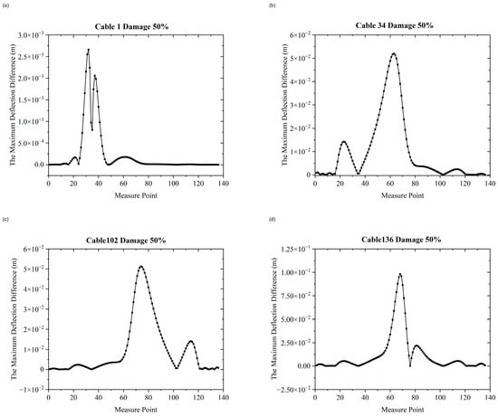
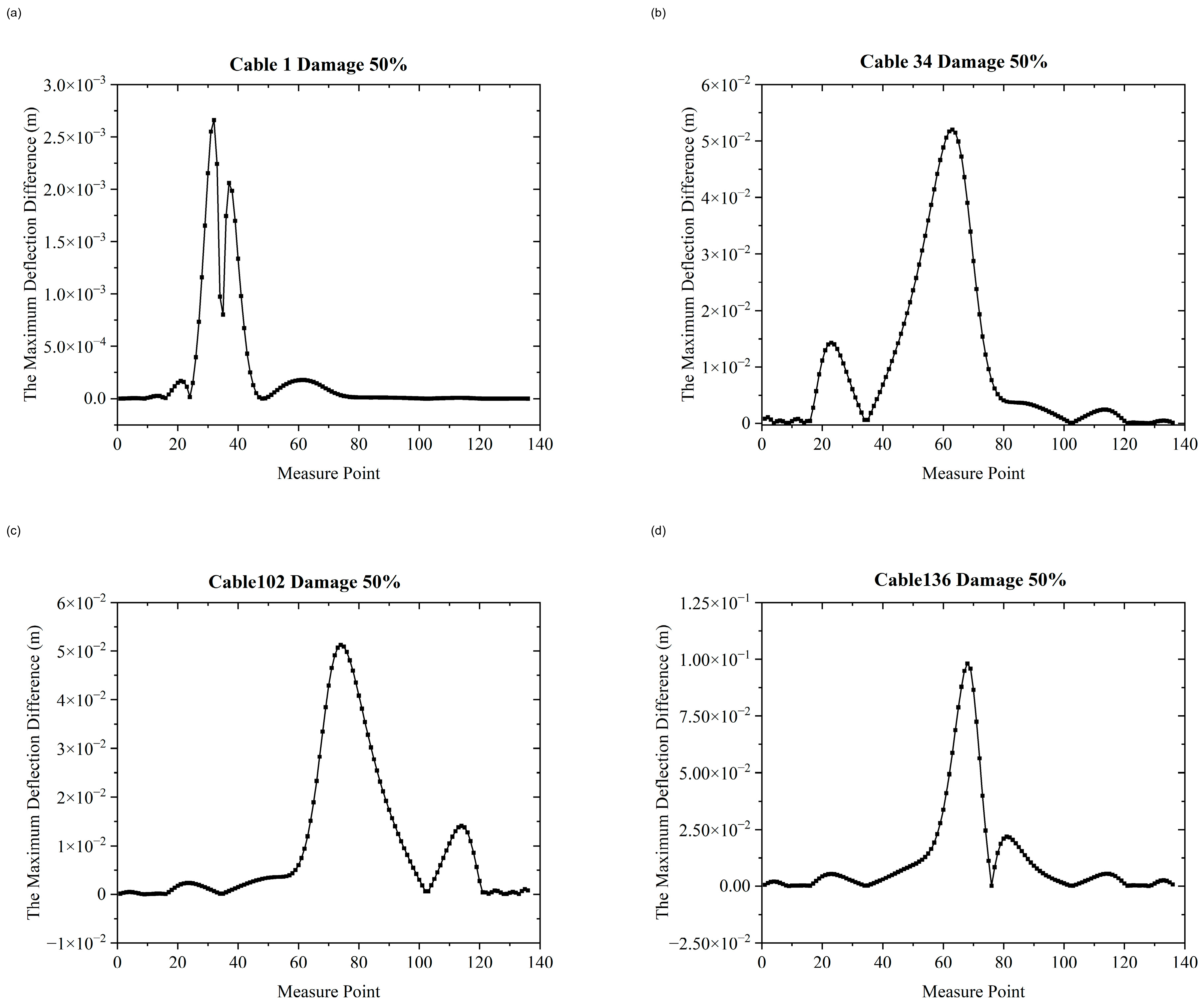
In long-span cable-stayed bridges, the main girder’s deflection indicates the condition of the stay cables. Consequently, a Damage Identification Index is derived from the bridge deck’s deflection at the cable anchor points. This study focuses on the cables on one side of the bridge, numbered 1 to 136 along the x-axis. Figure 6 illustrates the maximum disparity in the bridge deck’s deflection at all anchor points compared to the undamaged state, specifically when cables 1, 34, 102, and 136 experience a 50% reduction in cross-sectional area. In the implementation, for each anchor point j (j = 1, …, 136), the j_th DII component is calculated as ${\mathrm{DII}}_{\mathrm{j}}={\max }_{\mathrm{t}}|{\mathrm{u}}_{\mathrm{j}}^{\mathrm{damaged}}(\mathrm{t})-{\mathrm{u}}_{\mathrm{j}}^{\mathrm{intact}}(\mathrm{t})|$. Here, DII_j is the scalar DII value associated with anchor point j; ${\mathrm{u}}_{\mathrm{j}}^{\mathrm{damaged}}(\mathrm{t})$ and ${\mathrm{u}}_{\mathrm{j}}^{\mathrm{intact}}(\mathrm{t})$ are the deflections at anchor point j and recorded response time step t under the damaged and intact states, respectively; and t indexes the common set of aligned response time steps. The operator max_t selects the largest absolute difference over time, while |∙| retains the magnitude of the change and removes its sign. Therefore, DII_j has the same physical unit as the deflection response, and the 136 resulting scalar values, ordered by anchor point, form one 136-dimensional input feature vector. The maximum is not taken across anchor points or load cases. The intact and damaged cases use matched prescribed loading and model conditions. In a field implementation, the intact reference profile would be estimated from healthy monitoring periods and updated using synchronized environmental and operational variables or an updated numerical/measurement model before calculating DII. The different peak magnitudes in Figure 6 arise because each cable has a different influence on girder deflection as a result of its position, local stiffness, boundary restraint, and force redistribution through adjacent cables; therefore, equal percentage of area loss need not produce equal DII magnitudes at all cable locations.

Figure 6. Maximum differences in the deflections at each anchorage point between the bridge with 50% damage to cables 1, 34, 102, and 136 and the healthy bridge: (a) cable 1; (b) cable 34; (c) cable 102; (d) cable 136.

The figure illustrates that when identical damage occurs to various cables, the disparity between the deflection at each anchor point and that under healthy conditions changes significantly.

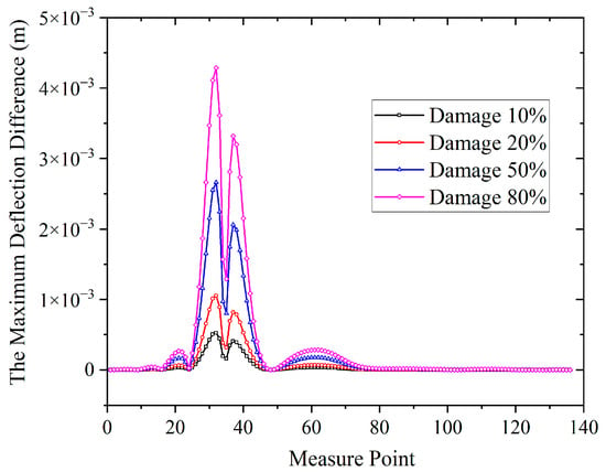
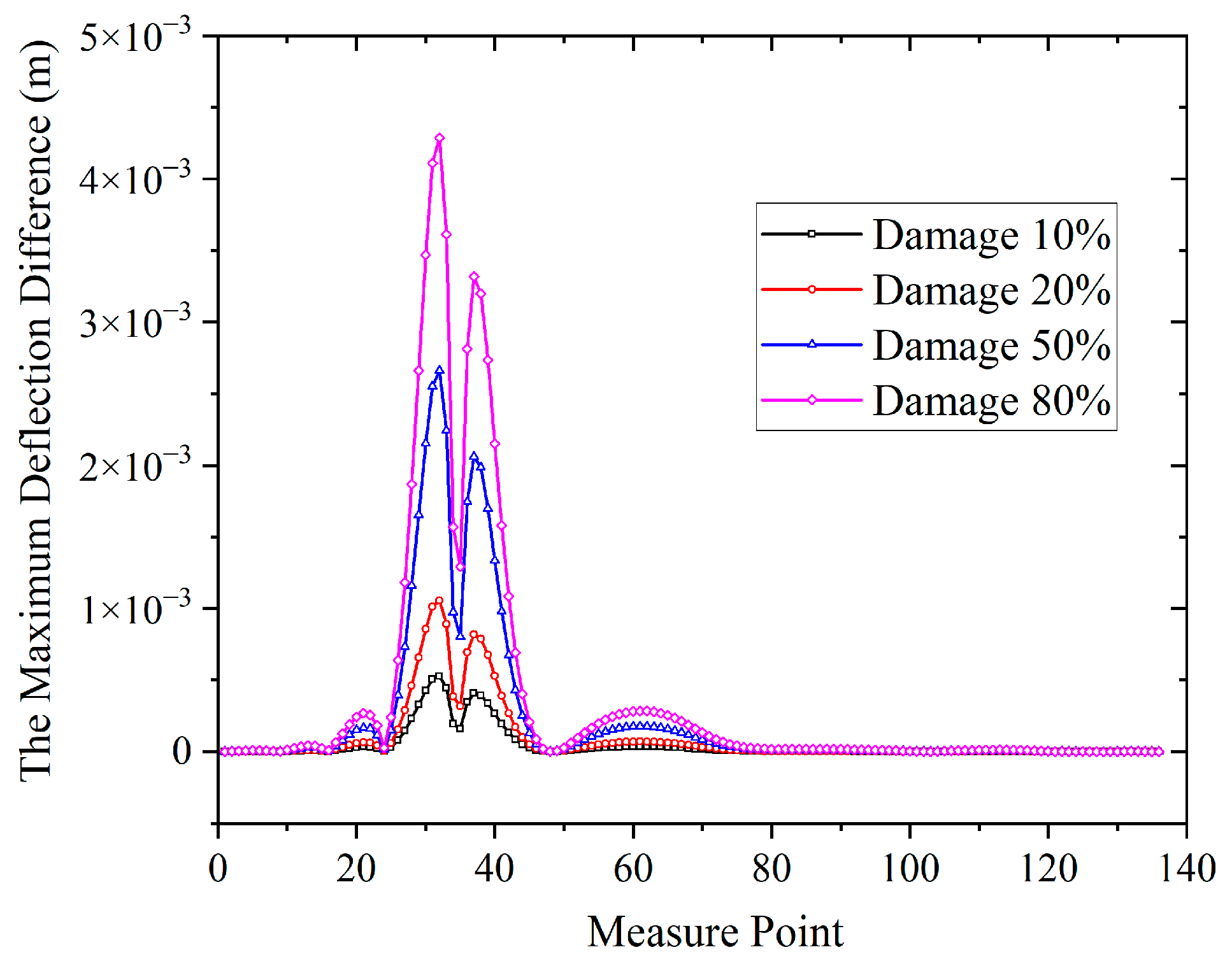
Based on the finite element method, the deflection difference distribution of cable 1 under damage severities of 10%, 20%, 50% and 80% is calculated, with the results shown in Figure 7. From the perspective of response magnitude, a 10% stiffness loss of the stay cable can induce a millimeter-scale deflection change at the anchor point, which is fully within the observable range of existing monitoring technologies. From the perspective of response characteristics, the stiffness degradation of a single stay cable will produce an extreme value characteristic of deflection increment at the corresponding anchor point, which can be used to locate the damaged cable and has clear identifiability. Hydrostatic leveling system, Fiber Bragg Grating (FBG) deflection sensors, and automated total station are the mainstream technologies for deflection monitoring of cable-stayed bridges, with a monitoring accuracy up to ±0.1 mm ~ ±0.5 mm [47,48]. The Damage Identification Index (DII) is a difference-type index, which can be calculated only with two sets of deflection data: the intact reference state and the current monitoring state. In summary, DII has favorable observability and stability, and can be used for damage identification of stay cables in cable-stayed bridges [31]. Therefore, in this study, “the maximum difference between the deflection at the anchor point in the damaged state of the stay cable and the deflection in the intact state” is taken as the Damage Identification Index for the localization of damaged stay cables. According to the analysis of Figure 7, the Damage Identification Index of cable 1 increases with the deepening of damage severity, and the variation law of the index at each anchor point is consistent. Hence, the identification of stay cable damage severity can be transformed into a regression problem for research.

Figure 7. Damage index diagrams for cable 1 at damage severities of 10%, 20%, 50%, and 80%.

Although the present numerical protocol uses all 136 cable-anchor locations, this configuration should be interpreted as a full-information benchmark rather than a requirement that every location be instrumented in routine practice. Bridge structural health monitoring studies commonly select a limited number of sensors using damage sensitivity, modal information, accessibility, redundancy, and cost, and then reconstruct or expand responses at unmeasured locations [45,47,48].

3.4. Data Preprocessing

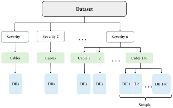
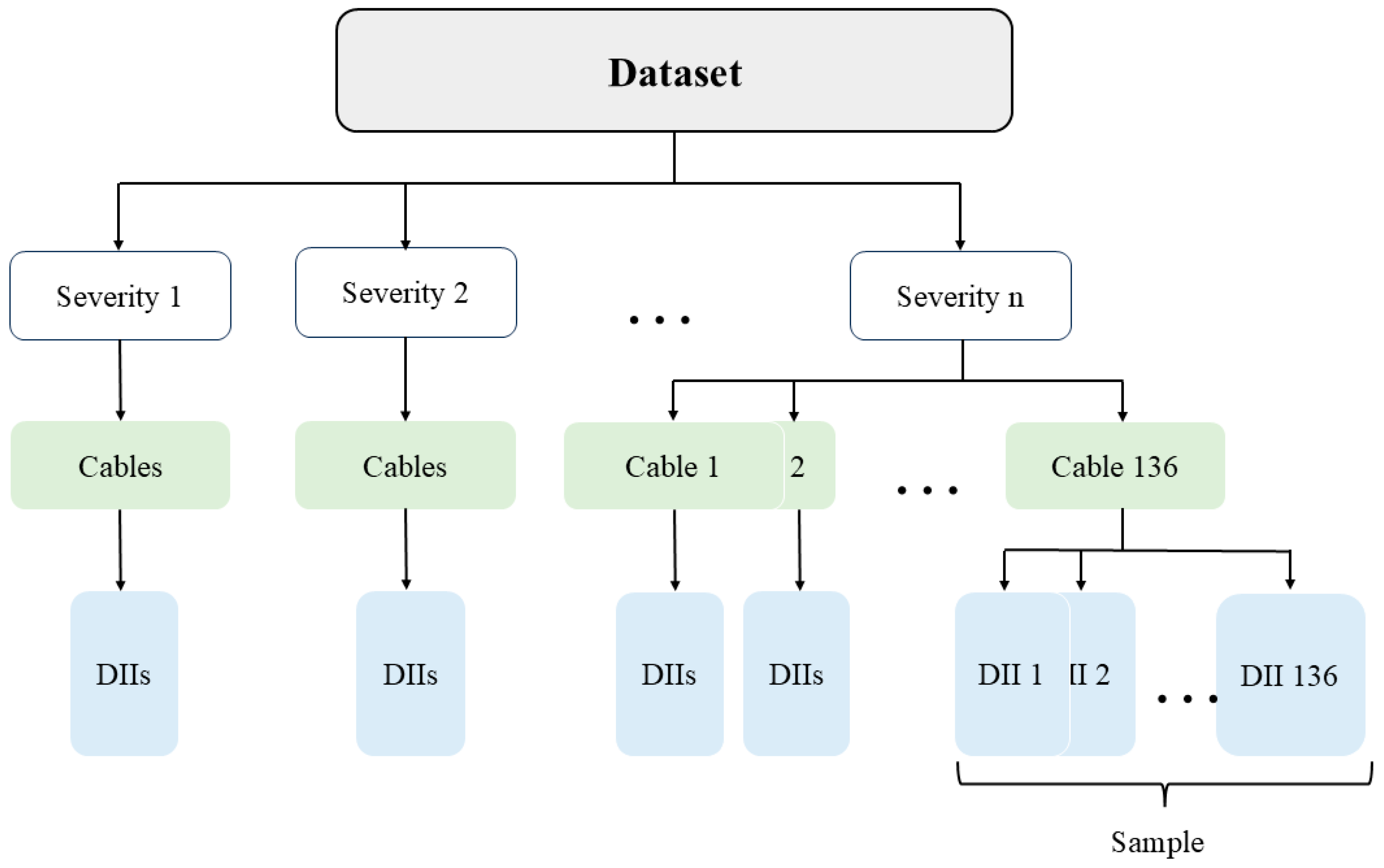
The deflection responses of the main girder under different stay cable damage conditions are calculated via the finite element model, with monitoring points set at 136 stay cable anchor points on the main girder. Each sample consists of the Damage Identification Index (DII) values of the 136 monitoring points, namely a 136-dimensional static feature. The development dataset contains 81 damage-severity levels spanning 0.0–80.0%, with a nominal step size of one percentage point. Each level contains 136 samples, giving 11016 development samples. The development samples are randomly divided at the individual-sample level into a training set and a validation set at a ratio of 8:2, corresponding to 8812 training samples and 2204 validation samples. After training and validation, the final model is evaluated using a separate independent test set. The independent test set contains the following 16 damage-severity levels, none of which is present in the development folders: 4.3%, 9.7%, 15.5%, 19.8%, 23.7%, 31.2%, 35.4%, 39.8%, 42.4%, 48.7%, 53.3%, 59.6%, 61.2%, 66.7%, 72.9%, and 78.1%. It contains 2176 samples in total, with 136 samples per level. The 16 independent severity levels were excluded from the development data before the 8:2 split was performed. Each processed severity folder contains one DII feature vector for each of the 136 cable-position scenarios. The dataset structure is shown in Figure 8.

Figure 8. Schematic diagram of the dataset structure.

The Z-score method is used to normalize the data [49]. The mean and standard deviation are fitted using the training subset only. The fitted parameters are then kept unchanged when transforming the validation set and the independent 16-level test set. This normalization method consists of three steps. The first step is to calculate the feature’s mean, as shown in Equation (14):

$${\mu }_j={\displaystyle \frac{1}{N_{\mathit{org}}}}{\sum }_{i=1}^{N_{\mathit{org}}}{x}_{i,j}$$

(14)

Among them, μ_j is the mean value of the features at the j_th monitoring point, N_org is the number of samples in the training subset, and x_ij is the maximum deflection difference at the j_th monitoring point in the i_th sample.

The second step is to calculate the standard deviation in the features, as shown in Equation (15):

$${\sigma }_j=\sqrt{{\displaystyle \frac{1}{N_{\mathit{org}}}}{\sum }_{i=1}^{N_{\mathit{org}}}{(x_{i,j}-{\mu }_j)}^2}$$

(15)

Among them, σ_j is the feature’s standard deviation in the j_th monitoring point.

Finally, performance of feature standardization transformation, that is, standardization of the original maximum deflection difference of the j_th sensor for the i_th sample of any dataset, is shown in Equation (16):

$$x_{i,j}^{\prime }={\displaystyle \frac{x_{i,j}-{\mu }_j}{{\sigma }_j}}$$

(16)

After this transformation, each dataset is fed into the model. The scaler fitted on the training subset is saved and reused without refitting for validation and independent testing, thereby preventing information leakage. The model’s hyperparameters are adjusted based on initial training performance. Table 1 presents the final hyperparameters of the optimized model. The hyperparameters were selected through an iterative tuning procedure informed by prior studies and feedback from the validation set. Candidate ranges were first defined for the number and width of hidden layers, dropout rate, batch size, initial learning rate, weight decay, and maximum number of training epochs, based on settings commonly used in related studies. Different candidate combinations were then compared over multiple training runs under a fixed data split, random seed, and training protocol. For DLIM, validation of position-identification accuracy was used as the primary selection criterion, whereas validation MAE was used for DSIM. The convergence of the training and validation losses, training stability, and the presence of apparent overfitting were also considered. The final network architectures and hyperparameter configurations were selected based on their validation performance, stable convergence, and comparatively favorable generalization behavior. The independent test set was reserved exclusively for final performance evaluation and was not used for hyperparameter or architecture selection.

Table 1. List of hyperparameters for DLIM and DSIM.

	Hyperparameter	DLIM	Candidate Range	DSIM	Candidate Range
Model	Fully connected layer dimension	[256,128,64]	[128,64], [256,128,64], [512,256,128,64]	[128,64]	[64,32], [128,64], [256,128]
	Dropout rate	0.3	[0.1,0.5]	0.4	[0.1,0.5]
	Spatial attention hidden layer dimension	128	64, 128, 256	128	64, 128, 256
Training	Batch size	128	[2,256]	128	[2,256]
	Epochs	80	[0,120]	100	[0,120]
	Patience	15	[10,30]	15	[10,30]
	Learning rate	3 × 10−3	5 × 10−4, 1 × 10−3, 3 × 10−3	1 × 10−3	5 × 10−4, 1 × 10−3, 3 × 10−3
	AdamW weight decay	5 × 10−5	[1 × 10−5, 3 × 10−4]	1 × 10−4	[1 × 10−5, 3 × 10−4]
	Cosine annealing scheduler period	80	[0,120]	100	[0,120]

4. Results

4.1. Identification of Damage Cable Location

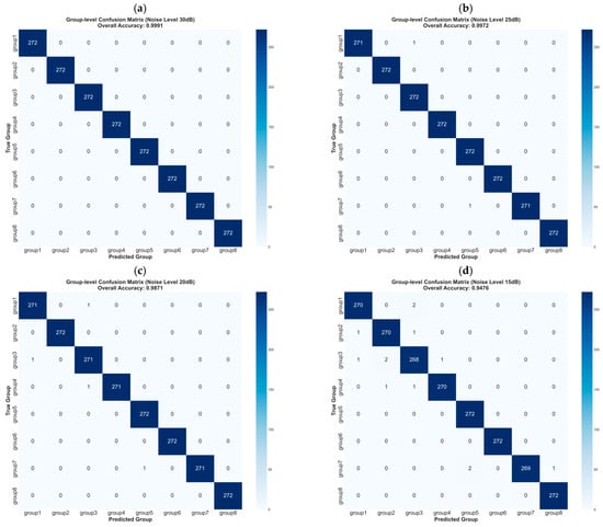
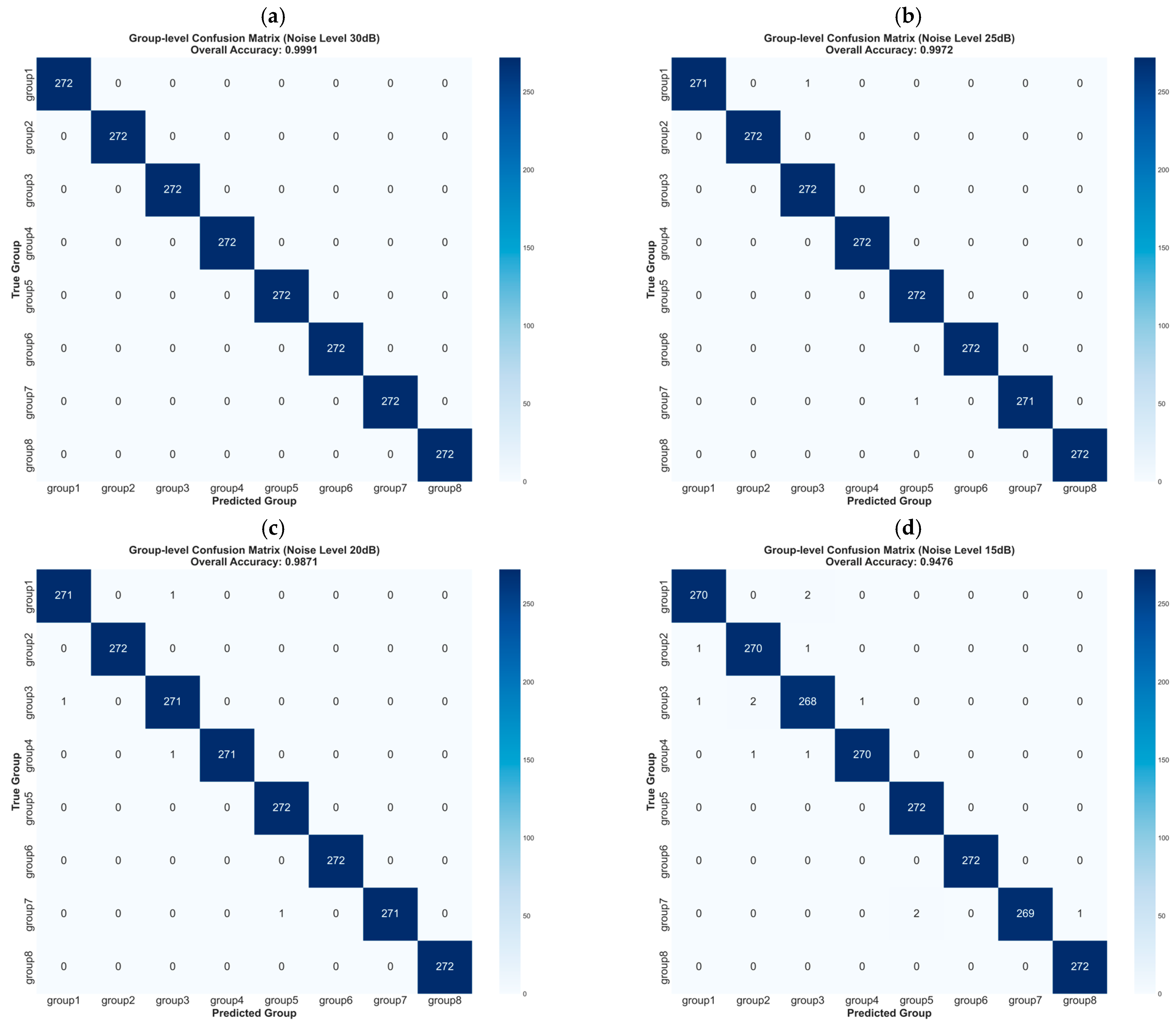
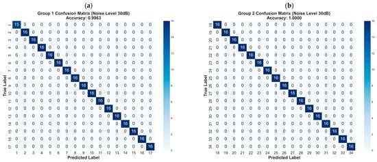
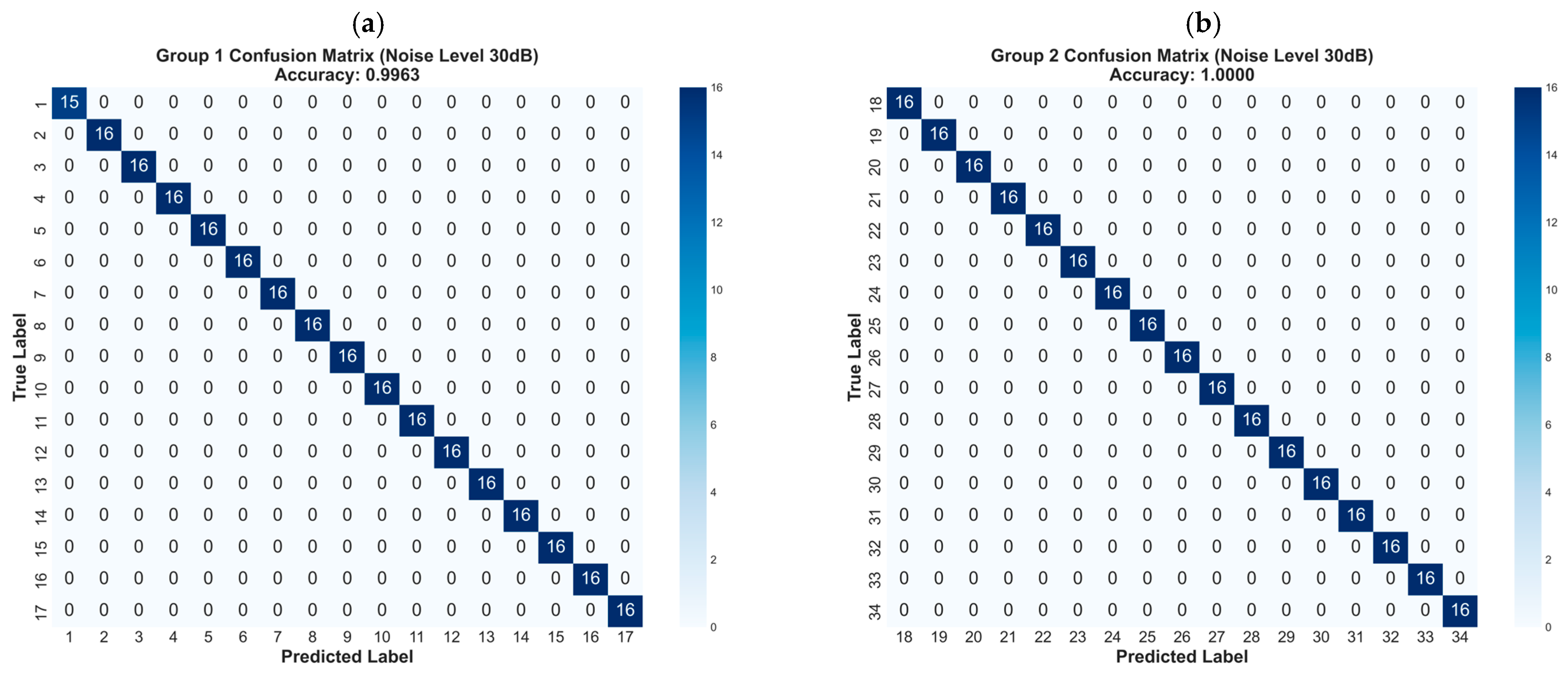
In this study, the stay cable damage conditions are divided into 136 categories, which are in one-to-one correspondence with the 136 stay cables on one side of the cable-stayed bridge, and this study focuses exclusively on the damage scenario of a single stay cable. Under the directional convention used here, the western side of the Sutong Bridge, corresponding to the upstream side of the Yangtze River, is designated as the upstream side; the opposite side is designated as downstream. The present model predicts the cable position on the modeled side. A two-dimensional localization procedure can therefore be applied first in a future two-side deployment, followed by the upstream/downstream designation. All model performance-related parameters presented in this chapter are obtained based on the independent test set containing the 16 unique damage severities listed in Section 3.4 (2176 samples in total, 136 samples per level). These levels are completely independent of the development folders and lie within the 1.0–80.0% range, so the reported evaluation is an interpolation test. The identification of damaged stay cables can be completed by inputting the test set into the trained model. Due to the large number of stay cables, the directly generated confusion matrix has low discriminability. To address this issue, all stay cables are divided into eight groups with 17 stay cables in each group, and the results of the damage identification model after grouping are shown in Figure 9a. The overall confusion matrix cannot fully reflect the actual identification accuracy, especially the intra-group misjudgment. Therefore, the confusion matrices of Group 1 and Group 2 are supplemented and presented in Figure 10, and the corresponding identification accuracy is detailed in Table 2.

Figure 9. Group-level confusion matrices of the Damage Location Identification Model under different signal-to-noise ratios: (a) 30 dB; (b) 25 dB; (c) 20 dB; (d) 15 dB.

Figure 10. Confusion matrices for damage-location prediction at SNR = 30 dB: (a) Group 1; (b) Group 2.

Table 2. Accuracy of each group under different noise levels.

Group	30 dB	25 dB	20 dB	15 dB
Group 1	99.63%	99.26%	98.53%	95.59%
Group 2	100.00%	100.00%	100%	96.69%
Group 3	99.63%	98.90%	97.43%	92.65%
Group 4	100.00%	100.00%	98.90%	94.85%
Group 5	100.00%	100.00%	99.63%	95.59%
Group 6	100.00%	100.00%	99.26%	96.69%
Group 7	100.00%	99.63%	98.16%	92.65%
Group 8	100.00%	100.00%	97.79%	93.38%
Average	99.91%	99.72%	98.71%	94.76%

Bridges are subjected to extensive noise interference during in-service operation; thus it is imperative to verify the noise robustness of the Damage Location Identification Model (DLIM). In this study, Additive White Gaussian Noise (AWGN) is adopted to perform noise contamination on the original noise-free Damage Identification Index (DII) sequences. The signal-to-noise ratio (SNR), with the unit of decibel (dB), is taken as the standardized quantitative indicator for noise level, and four gradient noise levels are set, namely 30 dB, 25 dB, 20 dB and 15 dB. Model testing is conducted separately using the abovementioned four noise-contaminated datasets. These results characterize controlled AWGN perturbations applied to the final DII only.

In the current implementation, the noise protocol is defined at the standardized DII-feature level. For each sample, let X = [x₁, x₂, …, x₁₃₆] denote the 136-dimensional DII feature vector after transformation using the scaler fitted on the training subset. Here, x_j is the standardized DII value corresponding to the j_th-ordered feature index, where j = 1, …, 136. The signal power is defined as

$$P_{\mathit{signal}}={\displaystyle \frac{1}{136}}{\displaystyle \sum _{j=1}^{136}}{x}_j^2$$

where P_signal represents the mean squared amplitude of the 136 feature components for the sample. The noise power is defined as

$$P_{\mathit{noise}}={\sigma }_n^2$$

where σ_n is the standard deviation in the zero-mean Gaussian noise and ${\sigma }_n^2$ is its variance. The target signal-to-noise ratio is calculated as

$$\mathit{SNR}\left(\mathrm{dB}\right)=10 {\mathit{log}}_{10}({\displaystyle \frac{P_{\mathit{signal}}}{P_{\mathit{noise}}}})$$

For a prescribed target SNR, the corresponding linear power ratio is 10^SNR/10, and the noise standard deviation is determined by

$${\sigma }_N=\sqrt{{\displaystyle \frac{P_{\mathit{signal}}}{{10}^{\frac{\mathit{SNR}}{10}}}}}$$

For each feature index, an independent zero-mean Gaussian noise sample is then generated as

$$n_j\sim \mathcal{N}\left(0,{\sigma }_n^2\right),$$

and the noisy input is calculated as

$${\tilde{x}}_j=x_j+n_j,$$

where n_j denotes the noise added to the j_th feature component and ${\tilde{x}}_j$ denotes the resulting noisy input feature. Both the position model and the severity model were trained with 30 dB AWGN augmentation, and the independent tests were conducted at 30, 25, 20, and 15 dB. Under the current protocol, one noise realization was generated for each sample and each SNR under a fixed random seed. No error was injected into the raw intact and damaged deflection responses before the DII was calculated.

Model calculation is performed on the noise-contaminated datasets, and the resulting confusion matrices are shown in Figure 9b–d. As the noise level increases, the identification accuracy of the model shows a slight decrease, and the vast majority of misclassifications occur within groups. This statement is obtained by inspecting the true-label and predicted-label entries in the exported test results and the resulting confusion matrices. Even under the noise level of SNR = 15 dB, the prediction accuracy of the model can still be maintained at 94.76%. Because the DII responses of adjacent stay cables are similar and the total number of stay cables is large, the observed errors are concentrated mainly among neighboring or same-group classes under the tested protocol.

To evaluate the effectiveness of the proposed MLP deep learning model integrated with the spatial attention module, comparisons are conducted between this model, the MLP model without the spatial attention module, the CNN model, and the RNN model. As a classic architecture for spatial feature extraction in deep learning, the CNN is also applicable to the damage identification task investigated in this study. It possesses the advantage of parallel computing and has been widely adopted in the field of bridge structural health monitoring (SHM). The RNN is capable of modeling the sequential dependence and long-range correlations of sequential data, making it well suited to the DII features mentioned in Section 3. In addition, it exhibits strong adaptability to noise-contaminated working conditions. The final tuned CNN model uses convolutional channels 64-128-256 with kernel size 3, a 128-unit fully connected head, dropout of 0.20, batch size of 128, AdamW with learning rate of 1 × 10⁻³ and weight decay of 5 × 10⁻⁵, 80 maximum epochs, patience of 15, and cosine annealing with T_max = 80. The final tuned RNN model uses a one-layer unidirectional LSTM with hidden size of 128, a 128-unit fully connected head, dropout of 0.20, and the same batch size, optimizer, learning rate, weight decay, patience and 80-epoch cosine schedule. These settings were selected under the same 8:2 training/validation protocol; the independent test set was not used for selection. At an SNR of 30 dB, the top-k accuracies of the four models are listed in Table 3.

Table 3. Identification accuracy comparison of different models at SNR = 30 dB.

	SAM-MLP Model	CNN Model	MLP Model Without SAM	RNN Model
Accuracy	99.91%	99.86%	99.77%	96.23%
Top-1 Accuracy	99.91%	99.86%	99.77%	96.23%
Top-3 Accuracy	100.00%	100.00%	100.00%	99.82%
Top-5 Accuracy	100.00%	100.00%	100.00%	100.00%
Top-10 Accuracy	100.00%	100.00%	100.00%	100.00%

Table 4 reports the identification accuracy of each model under the four tested noise levels. The SAM-MLP model achieved accuracies of 99.91%, 99.72%, 98.71%, and 94.76% at 30, 25, 20, and 15 dB, respectively. The corresponding accuracies were 99.77%, 99.36%, 98.02%, and 94.99% for the MLP without SAM, 99.86%, 99.54%, 97.47%, and 89.15% for tuned CNN model, and 96.23%, 92.60%, 80.74%, and 63.19% for tuned RNN model. Across the four SNR levels, the mean Top-1 accuracies are 98.28%, 96.51%, and 83.19% for SAM-MLP, CNN model, and RNN model, respectively. To highlight the principal comparison results, 30 dB and 15 dB were selected as representative noise levels, and relative accuracy changes were calculated using the corresponding comparison-model accuracies as the baselines. At 30 dB, the relative accuracy changes in SAM-MLP versus the MLP without SAM, CNN model, and RNN model were +0.14%, 0.05%, and +3.82%, respectively. At 15 dB, the corresponding relative increases were −0.24%, +6.29%, and +49.96%, respectively. The 25 dB and 20 dB results are consistent with the overall cross-SNR robustness pattern and are not expanded individually here due to space limitations.

Table 4. Identification accuracy of different models under various noise levels.

SNR	SAM-MLP Model	CNN Model	MLP Model Without SAM	RNN Model
30 dB	99.91%	99.86%	99.77%	96.23%
25 dB	99.72%	99.54%	99.36%	92.60%
20 dB	98.71%	97.47%	98.02%	80.74%
15 dB	94.76%	89.15%	94.99%	63.19%

4.2. Identification of Damage Cable Severity

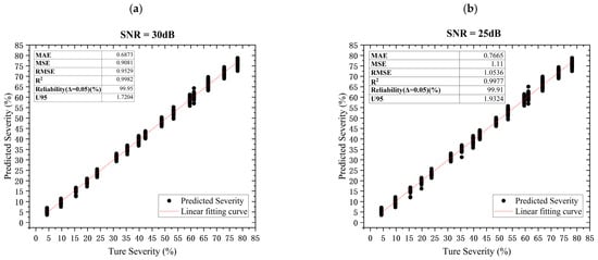
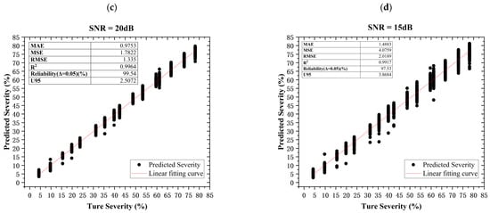
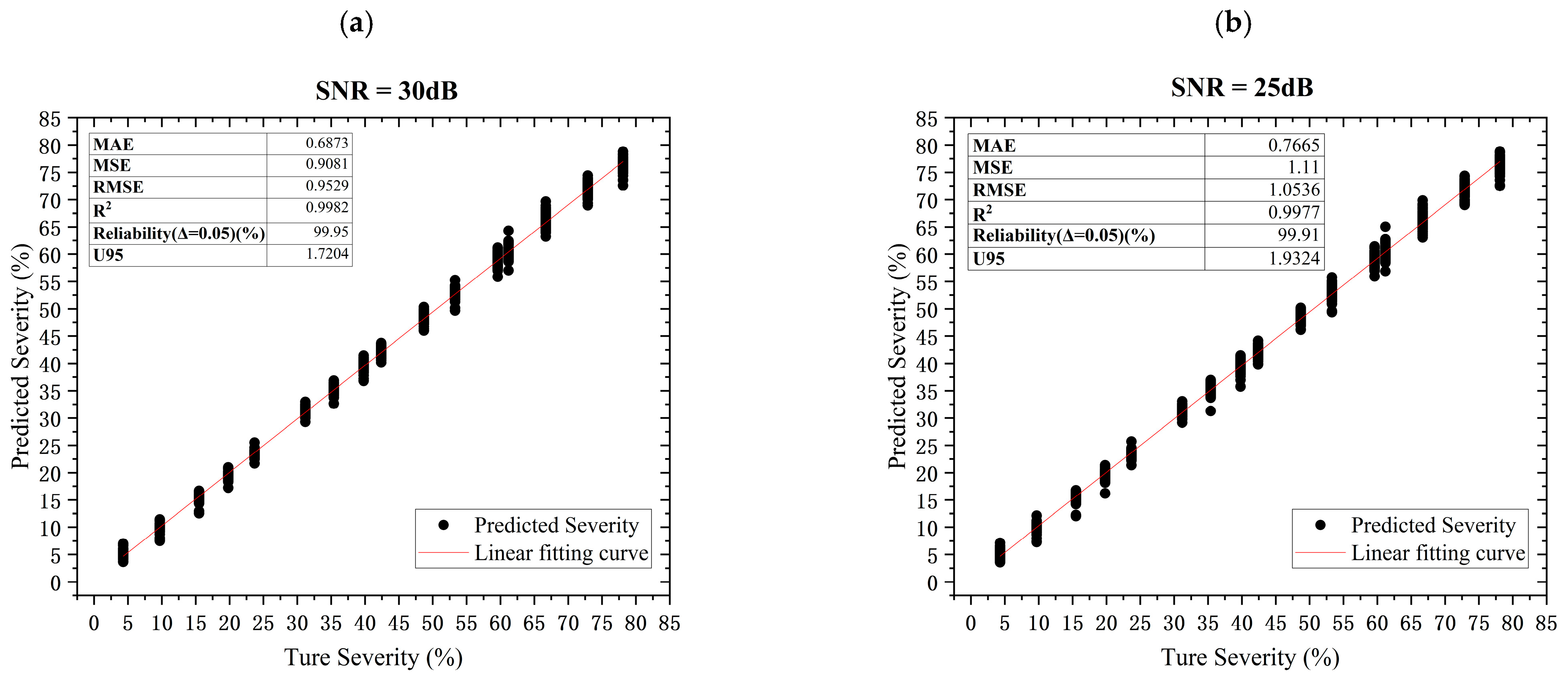
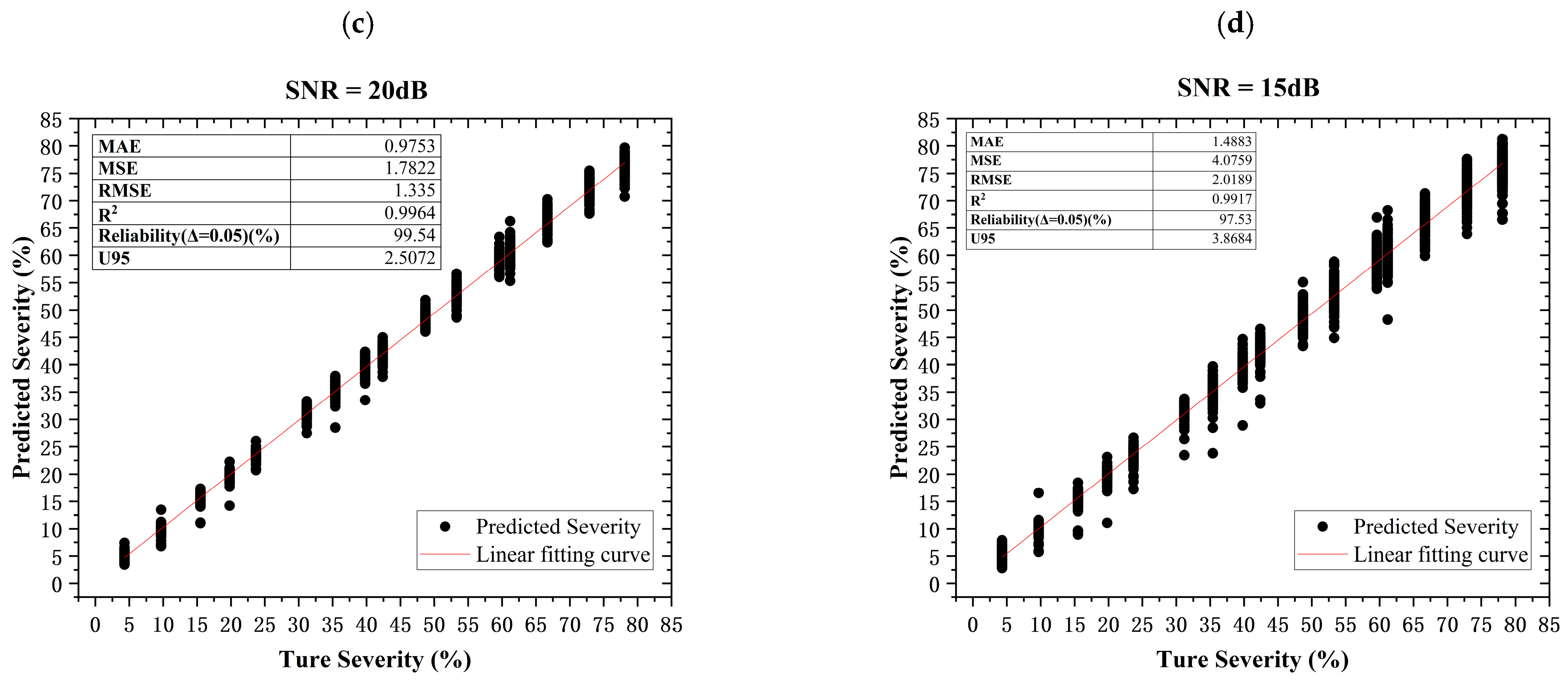
The Damage Severity Identification Model is a regression model whose target range is [0.0,80.0] percentage points; a value of 10.0 denotes 10% damage. Figure 11a compares predicted and true severity, and the evaluation procedures are described in Section 2.3.

Figure 11. Scatter plots of cable damage severity identification under different signal-to-noise ratios: (a) 30 dB; (b) 25 dB; (c) 20 dB; (d) 15 dB.

To evaluate noise robustness, tests were performed on independent test sets with noise levels of 30 dB, 25 dB, 20 dB and 15 dB. The corresponding scatter plots and evaluation indicators are presented in Figure 11b–d. As the noise level increases, MAE rises, with growth rates of 10.3%, 29.52% and 52.54% at 25 dB, 20 dB and 15 dB, respectively, while remaining below two percentage points. At 15 dB, MSE = 4.0759, RMSE = 2.0189, and R² = 0.9917. Reliability is 97.33%, meaning that 97.33% of samples have an absolute severity error no greater than five percentage points. U95 = 3.8684 and is calculated as 1.96 times the sample standard deviation in the residuals. Under an approximately normal residual distribution, this is an empirical 95% residual-spread summary; it is not a formal confidence interval. The five-percentage-point tolerance is a study-defined engineering tolerance on the percentage-point target. SHM reliability metrics and allowable errors are application-specific rather than universal [50,51,52]. Table 5 presents the evaluation metrics of the DSIM under different SNR conditions. The CNN model and RNN model results are reported separately in Table 6 so that the single-SNR comparison and the cross-SNR robustness results are not conflated.

Table 5. Model evaluation parameters under different noise levels.

	30 dB	25 dB	20 dB	15 dB
MAE	0.6873	0.7665	0.9753	1.4483
MSE	0.9081	1.1100	1.7822	4.0759
RMSE	0.9529	1.0536	1.3350	2.0189
R2	0.9982	0.9977	0.9964	0.9917
Reliability (%)	99.95	99.91	99.54	97.33
U95	1.7204	1.9324	2.5072	3.8684

Table 6. Comparison of evaluation parameters for different models at SNR = 30 dB.

	SAM-MLP Model	MLP Model Without SAM	CNN Model	RNN Model
MAE	0.6873	1.3674	0.6556	2.7576
MSE	0.9081	4.3021	0.7499	27.5160
RMSE	0.9529	2.0741	0.8660	5.2456
R2	0.9982	0.9912	0.9985	0.9441
Reliability (%)	99.95	96.32	100.00	87.32
U95	1.7204	3.9161	1.6819	10.2726

At SNR = 30 dB, the SAM-MLP model achieved an MAE of 0.6873, an MSE of 0.9081, an RMSE of 0.9529, an R² of 0.9982, a reliability of 99.95% (|e| ≤ five percentage points), and a U95 value of 1.7204. Because MAE, MSE, RMSE, and U95 are error metrics for which lower values indicate smaller prediction errors, SAM-MLP reduced these four metrics relative to the MLP without SAM by 49.74%, 78.89%, 54.06%, and 56.07%, respectively, and relative to RNN model by 75.08%, 96.70%, 81.83%, and 83.25%, respectively. In contrast, CNN model had lower single-SNR errors than SAM-MLP: its MAE, MSE, RMSE, and U95 were 4.8%, 21.09%, 10.03%, and 2.29% lower than those of SAM-MLP, respectively. For reliability, SAM-MLP was 3.63 percentage points above the MLP without SAM, 0.05 percentage points below CNN model, and 12.63 percentage points above RNN model. Although CNN model represents a clear exception at 30 dB, its performance deteriorates markedly at lower SNRs. At 25 dB, CNN model has an MAE of 1.7682 and a reliability of 94.67%, compared with 0.7665 and 99.91% for SAM-MLP. At 20 dB, the corresponding values are 6.5839 and 54.14% for CNN model, versus 0.9753 and 99.54% for SAM-MLP. At 15 dB, CNN model reaches an MAE of 20.4089 percentage points and a reliability of 6.89%, whereas SAM-MLP achieves 1.4483 and 97.33%, respectively. Thus, the cross-SNR results support interpreting SAM-MLP as the more stable and balanced model.

5. Conclusions

This study proposes a SAM-MLP model integrated with a spatial attention module. This model is applied to identify cable damage and assess damage severity based on the deflection of the main girder in long-span cable-stayed bridges. The finite element model (FEM) of the bridge is developed using OpenSees. This FEM is used to generate training, validation, and testing datasets for the Damage Location Identification Model (DLIM) and Damage Severity Identification Model (DSIM). The conclusions are as follows:

(1)

For the stay cable damage identification task characterized by a large number of cables and high similarity in damage features, the SAM-MLP model can effectively learn the inherent data characteristics. The trained DLIM achieves an identification accuracy of 99.91% for single damaged stay cables, and the accuracy still reaches 94.76% under the strong noise condition of SNR = 15 dB. The DSIM delivers good performance in damage severity evaluation. Under the high-noise condition of SNR = 15 dB, its identification reliability amounts to 97.33%, with a mean absolute error (MAE) of 1.4483 percentage points.

(2)

The tuned comparison study shows that model selection must be based on the full noise range rather than a single high-SNR value. Across 30, 25, 20, and 15 dB, the mean DLIM Top-1 accuracies are 98.28% for SAM-MLP, 96.51% for CNN model, 98.04% for MLP and 83.19% for RNN model. For DSIM, the corresponding mean MAE values are 0.9694, 7.3541, 1.7586 and 2.9102, and the mean reliability values are 99.18%, 63.92%, 93.65% and 85.63%. At 30 dB, CNN model has a lower DSIM MAE (0.6556 versus 0.6873). At 15 dB, SAM-MLP exceeds CNN model and RNN model in DLIM accuracy by 5.61 and 31.57 percentage points, respectively, and its DSIM MAE is 92.9% and 54.56% lower, respectively. The evidence therefore supports SAM-MLP as the more stable cross-SNR method rather than as the universally best model at every individual condition.

(3)

The proposed model maintained the reported performance under the tested AWGN conditions. The present study is limited to single-cable damage and FEM-generated data.

Within this numerical protocol, intact and damaged cases are compared under matched modeled loading and boundary conditions. A field implementation would require a state-conditioned reference profile or an updated numerical/measurement baseline to account for temperature, traffic, wind, boundary, and sensor variability.

References

- Sun, Z.K.; Li, G.M.; Geng, S.H. Study on stayed-cable health monitoring. In Intelligence Computation and Evolutionary Computation; Du, Z., Ed.; Springer: Berlin/Heidelberg, Germany, 2013; Volume 180, pp. 1091–1098. [Google Scholar] [CrossRef] [Scilit]
- Dong, J.; Yan, X.; Li, S. Cable force monitoring and prediction for cable group of long-span cable-supported bridges. J. Civ. Struct. Health Monit. 2018, 8, 597–605. [Google Scholar] [CrossRef] [Scilit]
- Zui, H.; Shinke, T.; Namita, Y. Practical formulas for estimation of cable tension by vibration method. J. Struct. Eng. 1996, 122, 651–656. [Google Scholar] [CrossRef] [Scilit]
- Casas, J.R. Full-scale dynamic testing of the Alamillo cable-stayed bridge in Sevilla (Spain). Earthq. Eng. Struct. Dyn. 1995, 24, 35–51. [Google Scholar] [CrossRef] [Scilit]
- Kim, B.H.; Park, T. Estimation of cable tension force using the frequency-based system identification method. J. Sound Vib. 2007, 304, 660–676. [Google Scholar] [CrossRef] [Scilit]
- Russell, J.C.; Lardner, T.J. Experimental determination of frequencies and tension for elastic cables. J. Eng. Mech. 1998, 124, 1067–1072. [Google Scholar] [CrossRef] [Scilit]
- Kamal, M.; Mansoor, A. Structural health monitoring and IoT: Opportunities and challenges. In Intelligence of Things: Technologies and Applications; Dao, N.-N., Le, H.A., Nguyen, N.T., Pham, Q.-D., Eds.; Springer International Publishing AG: Cham, Switzerland, 2022; Volume 148, pp. 3–15. [Google Scholar] [CrossRef] [Scilit]
- Cho, S.; Lynch, J.P.; Lee, J.-J.; Yun, C.-B. Development of an automated wireless tension force estimation system for cable-stayed bridges. J. Intell. Mater. Syst. Struct. 2010, 21, 361–376. [Google Scholar] [CrossRef] [Scilit]
- Li, J.; Wang, C.; Zhao, Y. A long-term monitoring method of corrosion damage of prestressed anchor cable. Micromachines 2023, 14, 799. [Google Scholar] [CrossRef] [Scilit] [PubMed]
- Abedin, S.; Biondi, A.M.; Cao, L.; Wu, R.; Yu, T.; Wang, X. A textile embedded with distributed fiber optic sensors for pedestrian bridge monitoring. In Experimental Vibration Analysis for Civil Engineering Structures; Limongelli, M.P., Gentile, C., Giordano, P.F., Quqa, S., Cigada, A., Eds.; Springer: Berlin/Heidelberg, Germany, 2023; Volume 433, pp. 689–695. [Google Scholar] [CrossRef] [Scilit]
- Guo, J.; Zhu, X. Field monitoring and analysis of the vibration of stay cables under typhoon conditions. Sensors 2020, 20, 4520. [Google Scholar] [CrossRef] [Scilit] [PubMed]
- Diamanti, K.; Soutis, C. Structural health monitoring techniques for aircraft composite structures. Prog. Aerosp. Sci. 2010, 46, 342–352. [Google Scholar] [CrossRef] [Scilit]
- Hao, H.; Xia, Y. Vibration-based damage detection of structures by genetic algorithm. J. Comput. Civ. Eng. 2002, 16, 222–229. [Google Scholar] [CrossRef] [Scilit]
- Lee, J.J.; Lee, J.W.; Yi, J.H.; Yun, C.B.; Jung, H.Y. Neural networks-based damage detection for bridges considering errors in baseline finite element models. J. Sound Vib. 2005, 280, 555–578. [Google Scholar] [CrossRef] [Scilit]
- Bakhary, N.; Hao, H.; Deeks, A.J. Damage detection using artificial neural network with consideration of uncertainties. Eng. Struct. 2007, 29, 2806–2815. [Google Scholar] [CrossRef] [Scilit]
- Chandrashekhar, M.; Ganguli, R. Damage assessment of structures with uncertainty by using mode-shape curvatures and fuzzy logic. J. Sound Vib. 2009, 326, 939–957. [Google Scholar] [CrossRef] [Scilit]
- Li, R.; Mita, A.; Zhou, J. Symbolization-based differential evolution strategy for identification of structural parameters. Struct. Control Health Monit. 2013, 20, 1255–1270. [Google Scholar] [CrossRef] [Scilit]
- Ding, Z.H.; Huang, M.; Lu, Z.R. Structural damage detection using artificial bee colony algorithm with hybrid search strategy. Swarm Evol. Comput. 2016, 28, 1–13. [Google Scholar] [CrossRef] [Scilit]
- Padil, K.H.; Bakhary, N.; Hao, H. The use of a non-probabilistic artificial neural network to consider uncertainties in vibration-based-damage detection. Mech. Syst. Signal Process. 2017, 83, 194–209. [Google Scholar] [CrossRef] [Scilit]
- Pathirage, C.S.N.; Li, J.; Li, L.; Hao, H.; Liu, W.; Ni, P. Structural damage identification based on autoencoder neural networks and deep learning. Eng. Struct. 2018, 172, 13–28. [Google Scholar] [CrossRef] [Scilit]
- Yeung, W.T.; Smith, J.W. Damage detection in bridges using neural networks for pattern recognition of vibration signatures. Eng. Struct. 2005, 27, 685–698. [Google Scholar] [CrossRef] [Scilit]
- Dackermann, U.; Smith, W.A.; Randall, R.B. Damage identification based on response-only measurements using cepstrum analysis and artificial neural networks. Struct. Health Monit. 2014, 13, 430–444. [Google Scholar] [CrossRef] [Scilit]
- Hou, R.; Xia, Y. Review on the new development of vibration-based damage identification for civil engineering structures: 2010–2019. J. Sound Vib. 2021, 491, 115741. [Google Scholar] [CrossRef] [Scilit]
- Sun, L.; Shang, Z.; Xia, Y.; Bhowmick, S.; Nagarajaiah, S. Review of bridge structural health monitoring aided by big data and artificial intelligence: From condition assessment to damage detection. J. Struct. Eng. 2020, 146, 04020073. [Google Scholar] [CrossRef] [Scilit]
- Ye, X.W.; Jin, T.; Yun, C.B. A review on deep learning-based structural health monitoring of civil infrastructures. Smart Struct. Syst. 2019, 24, 567–585. [Google Scholar] [CrossRef]
- Feng, D.-C.; Wang, W.-J.; Mangalathu, S.; Taciroglu, E. Interpretable XGBoost-SHAP machine-learning model for shear strength prediction of squat RC walls. J. Struct. Eng. 2021, 147, 04021173. [Google Scholar] [CrossRef] [Scilit]
- Kang, M.-S.; An, Y.-K. Crack growth prediction on a concrete structure using deep ConvLSTM. Smart Struct. Syst. 2024, 33, 301–311. [Google Scholar] [CrossRef]
- Wang, X.; Wang, Z.; Yang, S.; Wei, S.; Wang, T.; Shahzad, M.M. An incremental broad ensemble learning framework for the identification of structural damage in conditions of data scarcity and non-stationarity. Eng. Struct. 2026, 353, 122261. [Google Scholar] [CrossRef] [Scilit]
- Wang, X.; Wei, Z.; Wang, Z.; Wei, S.; Li, Y. Explainable AI-Driven Optimal Feature Selection for the Identification of Structural Damage. Struct. Control Health Monit. 2025, 2025, 7253150. [Google Scholar] [CrossRef] [Scilit]
- Wang, X.; Shahzad, M.M.; Wei, Z.; Yang, S.; Wang, T. Transfer Learning-Enhanced Residual Attention Temporal Network for Structural Damage Identification. Buildings 2026, 16, 2779. [Google Scholar] [CrossRef] [Scilit]
- Ren, J.; Zhang, B.; Zhu, X.; Li, S. Damaged cable identification in cable-stayed bridge from bridge deck strain measurements using support vector machine. Adv. Struct. Eng. 2022, 25, 754–771. [Google Scholar] [CrossRef] [Scilit]
- Wang, H.; Wang, Z.; Zhang, F.; Xu, Y.; Zhang, Y.; Shen, K.; Meng, X.; Wang, J. Multi-loads response prediction for long-span cable-stayed bridges by integrating physical model updating and deep learning. Adv. Struct. Eng. 2026. [Google Scholar] [CrossRef] [Scilit]
- Zeng, Y.; Du, J.; Zhang, J.; Wang, J.; Fan, J. Identification of cable-stayed bridge damage based on anchor point vibrations caused by moving vehicle loads and through machine learning. J. China Foreign Highw. 2026, 46, 177–187. [Google Scholar] [CrossRef]
- Cianci, E.; Civera, M.; De Biagi, V.; Chiaia, B. Physics-informed machine learning for the structural health monitoring and early warning of a long highway viaduct with displacement transducers. Mech. Syst. Signal Process. 2026, 242, 113659. [Google Scholar] [CrossRef] [Scilit]
- Martucci, D.; Civera, M.; Surace, C. Bridge monitoring: Application of the extreme function theory for damage detection on the I-40 case study. Eng. Struct. 2023, 279, 115573. [Google Scholar] [CrossRef] [Scilit]
- Wang, R.; Wang, M.; Zhang, Z.; Xing, J.; Liu, X. LLNet: Lightweight network with a channel and spatial attention mechanism for local climate zone classification from Sentinel-2 image. Int. J. Climatol. 2023, 43, 1543–1560. [Google Scholar] [CrossRef] [Scilit]
- Svozil, D.; Kvasnicka, V.; Pospichal, J. Introduction to multi-layer feed-forward neural networks. Chemom. Intell. Lab. Syst. 1997, 39, 43–62. [Google Scholar] [CrossRef] [Scilit]
- Hastie, T.J.; Tibshirani, R.J.; Friedman, J.H. The Elements of Statistical Learning: Data Mining, Inference, and Prediction, 2nd ed.; corrected 7th printing; Springer: Berlin/Heidelberg, Germany, 2009. [Google Scholar] [CrossRef]
- Hecht-Nielsen. Theory of the backpropagation neural network. In International 1989 Joint Conference on Neural Networks; IEEE: New York, NY, USA, 1989; Volume 1, pp. 593–605. [Google Scholar] [CrossRef] [Scilit]
- Van Der Malsburg, C. Frank Rosenblatt: Principles of neurodynamics: Perceptrons and the theory of brain mechanisms. In Brain Theory; Aertsen, A., Palm, G., Eds.; Springer: Berlin/Heidelberg, Germany, 1986; pp. 245–248. [Google Scholar] [CrossRef] [Scilit]
- Ramachandran, P.; Zoph, B.; Le, Q.V. Searching for activation functions. arXiv 2017, arXiv:1710.05941. [Google Scholar] [CrossRef] [Scilit]
- Zhu, X.; Cheng, D.; Zhang, Z.; Lin, S.; Dai, J. An empirical study of spatial attention mechanisms in deep networks. In Proceedings of the IEEE International Conference on Computer Vision, Seoul, Republic of Korea, 27 October–2 November 2019; p. 9009578. [Google Scholar] [CrossRef] [Scilit]
- Wu, Y.-X.; Du, K.; Wang, X.-J.; Min, F. Misclassification-guided loss under the weighted cross-entropy loss framework. Knowl. Inf. Syst. 2024, 66, 4685–4720. [Google Scholar] [CrossRef] [Scilit]
- Moraes, A.M.; Pugliese, L.F.; dos Santos, R.F.; Vitor, G.B.; Braga, R.A.d.S.; da Silva, F.R. Effectiveness of YOLO architectures in tree detection: Impact of hyperparameter tuning and SGD, Adam, and AdamW optimizers. Standards 2025, 5, 9. [Google Scholar] [CrossRef] [Scilit]
- Ghannadi, P.; Kourehli, S.S. An effective method for damage assessment based on limited measured locations in skeletal structures. Adv. Struct. Eng. 2021, 24, 183–195. [Google Scholar] [CrossRef] [Scilit]
- JTG/T 3360-01-2018; Wind-Resistant Design Specification for Highway Bridges. Ministry of Transport of the People’s Republic of China: Beijing, China, 2018. Available online: https://xxgk.mot.gov.cn/jigou/glj/202006/t20200623_3313096.html (accessed on 28 August 2026). (In Chinese)
- Deng, Z.; Huang, M.; Wan, N.; Zhang, J. The current development of structural health monitoring for bridges: A review. Buildings 2023, 13, 1360. [Google Scholar] [CrossRef] [Scilit]
- He, Z.; Li, W.; Salehi, H.; Zhang, H.; Zhou, H.; Jiao, P. Integrated structural health monitoring in bridge engineering. Autom. Constr. 2022, 136, 104168. [Google Scholar] [CrossRef] [Scilit]
- Jain, S.; Shukla, S.; Wadhvani, R. Dynamic selection of normalization techniques using data complexity measures. Expert Syst. Appl. 2018, 106, 252–262. [Google Scholar] [CrossRef] [Scilit]
- Sankararaman, S.; Mahadevan, S. Uncertainty quantification in structural damage diagnosis. Struct. Control Health Monit. 2011, 18, 807–824. [Google Scholar] [CrossRef] [Scilit]
- Falcetelli, F.; Yue, N.; Di Sante, R.; Zarouchas, D. Probability of detection, localization, and sizing: The evolution of reliability metrics in Structural Health Monitoring. Struct. Health Monit. 2022, 21, 2990–3017. [Google Scholar] [CrossRef] [Scilit]
- Li, Z.; Lin, W.; Zhang, Y. Drive-by bridge damage detection using Mel-frequency cepstral coefficients and support vector machine. Struct. Health Monit. 2023, 22, 3302–3319. [Google Scholar] [CrossRef] [Scilit]
Disclaimer/Publisher’s Note: The statements, opinions and data contained in all publications are solely those of the individual author(s) and contributor(s) and not of MDPI and/or the editor(s). MDPI and/or the editor(s) disclaim responsibility for any injury to people or property resulting from any ideas, methods, instructions or products referred to in the content. |
© 2026 by the authors. Licensee MDPI, Basel, Switzerland. This article is an open access article distributed under the terms and conditions of the Creative Commons Attribution (CC BY) license.