Reflected Wave Method for Predicting the Joint Ahead of an Excavation Face in Soft–Hard Interbedded Strata

Abstract

This study investigates the influence of the wave impedance ratio on the accuracy of joint location predictions in soft–hard interbedded rock mass (SHIRM) using the reflected wave method. The propagation of stress waves across a joint is simulated by integrating the standard linear solid model with the displacement discontinuity model. Predictions were made in SHIRM for two cases: hard rock mass to soft rock mass and soft rock mass to hard rock mass, with twenty-two conditions of wave impedance ratios considered. The influence of incident wave amplitude, frequency, and joint stiffness on prediction relative error was systematically evaluated. The results show that the relative error first decreases and then increases as the wave impedance ratio increases in the case of hard rock mass to soft rock mass, while the opposite trend occurs as the ratio increases in the case of soft rock mass to hard rock mass. Prediction error is found to be insensitive to changes in wave amplitude across all impedance ratios tested. Furthermore, an applicable frequency range is determined, within which the relative error remains below 5% for wave impedance ratio conditions in the case of hard rock mass to soft rock mass, and below 10% for ratios in the case of soft rock mass to hard rock mass. Additionally, for stiffness values between 1 and 10 GPa and wave impedance ratios in the case of hard rock mass to soft rock mass, the relative error stays consistently under 5%.

1. Introduction

The stability of rock mass represents a fundamental concern in rock engineering, as it is predominantly governed by the presence of weak structural planes such as joints and fractures [1,2]. The spatial location of these planes significantly influences both the permeability and mechanical strength of the rock mass. Engineering hazards, including slippage and water outbursts, frequently initiate along these structural interfaces due to external loading or other engineering disturbances [3,4,5,6]. Consequently, accurately determining the location of joints is crucial for stability analysis and risk mitigation [7].

Conventional approaches for locating joints include surface geological surveys, which are effective for mapping exposed discontinuities but cannot detect those within the rock mass interior [8,9,10,11]. Alternatively, drilling methods provide direct, accurate information through core sampling along the borehole trajectory [12,13,14]. However, increasing the density of boreholes to improve spatial coverage entails high costs, extended timelines, and inherent damage to the rock mass, limiting the practicality of this approach [15,16]. Advancements in geophysical detection have promoted the use of seismic reflection methods, which utilize stress wave propagation to non-invasively identify internal joints [3,11,17,18]. This technique relies on the transmission and reflection of stress waves at mechanical interfaces [19]. By analyzing direct and reflected wave signals recorded at monitoring points, the position of a joint ahead of an excavation face can be inferred: direct waves constrain the wave velocity, while reflected waves are used to predict the location of the reflecting interface [3,20]. In conventional geological settings, stress waves are often simplified as elastic waves propagating at a constant velocity [21]. However, under complex in situ conditions, several physical factors can distort wave signals and compromise prediction accuracy.

In environments where the rock mass is subjected to coupled thermal, mechanical, and hydraulic processes, the induced micro-defects alter wave propagation characteristics [22,23,24]. This can lead to a propagation distance-dependent wave velocity, a phenomenon that necessitates treating the rock as a viscoelastic medium in such contexts [25,26,27,28]. Therefore, accounting for velocity dispersion becomes essential when applying wave-based detection in micro-defected rock. Another significant complication arises in heterogeneous stratigraphy, such as soft–hard interbedded rock mass (SHIRM), where pronounced lithological contrasts exist across discontinuities [29,30,31,32]. When a stress wave encounters such a discontinuity, the wave impedance ratio of the rock mass governs its reflection and transmission behavior, ultimately shifting the arrival time of the reflected wave peak [33,34,35,36]. Since accurate peak-time picking is a critical parameter for distance calculation in the reflection method, the impedance ratio may substantially influence the precision of joint localization [17]. Despite its potential impact, systematic research on the effect of the wave impedance ratio on the performance of the reflected wave method remains notably limited.

This study investigates the influence of the wave impedance ratio on the prediction accuracy of joint locations in SHIRM with micro-defects. The propagation of stress waves in such media is analytically and numerically examined. The reflected wave method is subsequently applied to predict the distance to joints across a defined range of wave impedance ratios. The effects of incident wave amplitude and frequency, as well as the stiffness of joint, on the relative prediction error are quantitatively evaluated under varying impedance conditions.

2. Identification Method and Wavefield Modeling

This section presents the identification method and wavefield modeling for locating a joint in soft–hard interbedded rock mass (SHIRM) containing micro-defects. The identification method derives the prediction equation for the joint distance, and the wavefield modeling describes the stress wave propagation by adopting the standard linear solid model for the micro-defected SHIRM, the displacement discontinuity model (DDM) for the joint boundary conditions, and the ray theory for tracing the reflected stress wave.

2.1. Location Identification Method

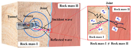
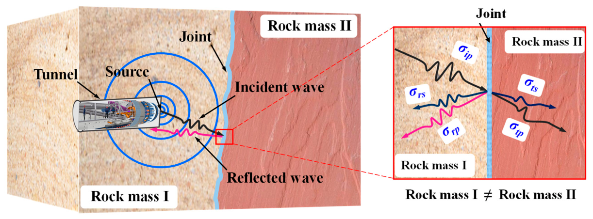
Figure 1 shows the SHIRM containing a joint, which exhibits distinct wave impedance on either side of the joint. The reflection and transmission behavior of the stress wave occurs when the stress wave generated by the source encounters such a joint.

Figure 1. Soft–hard interbedded rock mass (SHIRM) containing a joint.

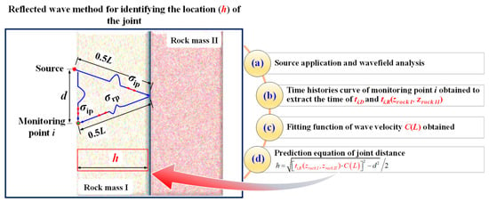
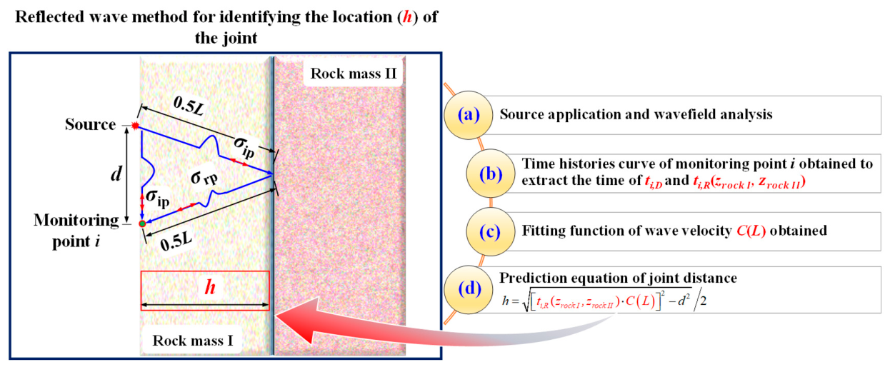
Figure 2 illustrates the procedure of the reflected wave method for locating the joint in soft–hard interbedded rock mass (SHIRM) containing micro-defects. It can be seen that the seismic source is applied to generate the stress wave and the wavefield in SHIRM with micro-defects containing a joint is analyzed. The time histories curve of stress wave at monitoring i is obtained and the arrived peak time of the directed P-wave (t_i,D) and reflected P-wave (t_i,R) is extracted. Therefore, the wave velocity can be calculated by the t_i,D and the fitting function C(L) between the wave velocity and the propagation distance is obtained. Finally, the predicted distance of the joint (h) can be calculated by the prediction equation of the reflected wave method. In Figure 2, z_{rock I} and z_{rock II} denote the wave impedances of the rock masses on the two sides of the joint, respectively, where the wave impedance is defined as the product of the medium density and the wave velocity. The arrival time of the reflected P-wave (t_i,R) is expressed as a function of these wave impedances because the impedance contrast governs the reflection and transmission behavior of the stress wave at the joint, and thus affects the peak arrival time of the reflected wave.

Figure 2. Process of reflected wave method for identifying the location of the joint in SHIRM containing micro-defects.

The propagation distance of the stress P-wave from the source to the joint and then reflected to the monitoring point i can be calculated from the relationship between the wave velocity obtained at the monitoring points and the peak arrival time of the reflected P-wave at monitoring point i follows:

L_i = C(L_i) ⋅ t_i,R

(1)

where C(L_i) is the fitting equation between the wave velocity and the propagation distance. The fitting equation C(L) takes the form C(L) = a₀ + a₁exp(a₂L), where a₀, a₁, and a₂ are fitting coefficients determined by fitting the wave velocities calculated from the direct wave arrival time at different propagation distances; t_i,R is the peak arrival time of the reflected P-wave at monitoring point i.

In addition, the propagation distance also satisfies

$$L_i=\sqrt{d_i^2+4h^2}$$

(2)

where h represents the distance between the joint and the source; d_i is the distance between the source and monitoring point i.

Therefore, according to Equations (1) and (2), the distance can be predicted by the monitoring point i as

$$h={\displaystyle \frac{\sqrt{{\left[t_{i,R}\cdot C\left(L_i\right)\right]}^2-d_i^2}}{2}}$$

(3)

2.2. Wavefield Modeling

The propagation of stress waves through soft–hard interbedded rock mass (SHIRM) containing micro-defects and a joint can be effectively represented by wave transmission across a discontinuous interface within an equivalent viscoelastic medium system. In this paper, the DDM is adopted to describe the boundary conditions of stress and displacement when the stress wave propagates through the joint. Standard linear solid models are adopted to describe SHIRM with micro-defects. To obtain the time history curve of the stress wave at monitoring point i based on the ray theory of stress waves, the following procedure is used. The incident stress P-wave first propagates from the source to the joint. The transmission and reflection of the stress P-wave occur at the joint under oblique incidence. The reflected stress P-wave finally propagates from the joint to the monitoring point i. It should be noted that the present study adopts the ray theory framework to trace the specific ray path. Within this framework, the one-dimensional form of the wave equation is used solely to derive the local propagation parameters along the ray direction, namely, the wavenumber and attenuation coefficient, which describe the amplitude decay and phase shift of a harmonic wave traveling along the ray. These parameters are local properties of the equivalent viscoelastic medium at a given frequency. The two-dimensional geometric features of the problem, including the oblique incidence at the joint, the reflection and transmission angles, and the normal and tangential stress decomposition at the joint, are handled through Snell’s law and the stress-displacement boundary conditions at the joint. The specific equation for the propagation of the stress wave is derived as follows.

For simplicity, the propagation direction of the stress P-wave is denoted as the positive direction of the x-axis. The continuity equation of the stress wave can be written as

$${\displaystyle \frac{\partial v}{\partial x}}={\displaystyle \frac{\partial \epsilon }{\partial t}}$$

(4)

where ε and v, respectively, denote the strain and particle velocity; t is time.

The motion equation can be written as

$$\rho {\displaystyle \frac{\partial v}{\partial t}}={\displaystyle \frac{\partial \sigma }{\partial x}}$$

(5)

where ρ and σ, respectively, denote the density of the rock mass and stress.

The stress–strain relationship of the standard linear solid model [37] can be written as

$${\displaystyle \frac{\partial \epsilon }{\partial t}}+{\displaystyle \frac{E_a{E}_M}{(E_a+E_M)\eta }}\epsilon ={\displaystyle \frac{E_M}{E_a+E_M}}\left({\displaystyle \frac{1}{E_M}}{\displaystyle \frac{\partial \sigma }{\partial t}}+{\displaystyle \frac{\sigma }{\eta }}\right)$$

(6)

where E_M and η, respectively, denote the Maxwell element’s elastic modulus and viscous coefficient. E_a represents elastic modulus of a spring connected in parallel to the Maxwell element.

When Equation (6) is differentiated to x and Equations (4) and (5) are considered, the equation can be rewritten as

$${\displaystyle \frac{{\partial }^{2}v}{\partial x^2}}+{\displaystyle \frac{E_a{E}_M}{(E_a+E_M)\eta }}{\displaystyle \int \frac{{\partial }^{2}v}{\partial x^2}}\mathit{dt}-{\displaystyle \frac{\rho }{E_a+E_M}}{\displaystyle \frac{{\partial }^{2}v}{\partial t^2}}-{\displaystyle \frac{\rho E_M}{\left(E_a+E_M\right)\eta }}{\displaystyle \frac{\partial v}{\partial t}}=0$$

(7)

In this paper, the half-sine P-wave is adopted as the source, and the Fourier transform is used to discretize the half-sine wave into a series of harmonic waves. Taking a single-frequency harmonic as an example, the harmonic solution of Equation (7) has the following form [33]:

v(x,t) = Aexp(−αx)exp[i(ωt − kx)]

(8)

where A denotes the amplitude of particle velocity. ω = 2πf, and f denotes the frequency of the harmonic. k is the wavenumber, and α is the attenuation coefficient. k and α are, respectively, expressed as follows:

$$k^2={\displaystyle \frac{\rho {\omega }^2}{2E_a}}\left\{{\left[{\displaystyle \frac{1+{\omega }^2{\theta }_M^2}{1+{\left(1+\frac{E_M}{E_a}\right)}^2{\omega }^2{\theta }_M^2}}\right]}^{1/2}+{\displaystyle \frac{1+\left(1+\frac{E_M}{E_a}\right){\omega }^2{\theta }_M^2}{1+{\left(1+\frac{E_M}{E_a}\right)}^2{\omega }^2{\theta }_M^2}}\right\}$$

(9)

and

$${\alpha }^2={\displaystyle \frac{\rho {\omega }^2}{2E_a}}\left\{{\left[{\displaystyle \frac{1+{\omega }^2{\theta }_M^2}{1+{\left(1+\frac{E_M}{E_a}\right)}^2{\omega }^2{\theta }_M^2}}\right]}^{1/2}-{\displaystyle \frac{1+\left(1+\frac{E_M}{E_a}\right){\omega }^2{\theta }_M^2}{1+{\left(1+\frac{E_M}{E_a}\right)}^2{\omega }^2{\theta }_M^2}}\right\}$$

(10)

where θ_M = η/E_M denotes the relaxation time.

Therefore, when the harmonic propagates from the source to the joint, the incident wave at the joint can be calculated as

v_ip(L,t) = Aexp(−αL)exp[i(ωt − kL)]

(11)

where ν_ip is the particle velocity of the incident P-wave; L is the propagation distance from the source to the joint.

According to Snell’s law, the angles of each wave at the joint are as follows:

$${\displaystyle \frac{\sin {\alpha }_0}{V_{p1}}}={\displaystyle \frac{\sin {\alpha }_1}{V_{p1}}}={\displaystyle \frac{\sin {\alpha }_2}{V_{s1}}}={\displaystyle \frac{\sin {\alpha }_3}{V_{p2}}}={\displaystyle \frac{\sin {\alpha }_4}{V_{s2}}}$$

(12)

where α₀, α₁, α₂, α₃, and α₄ denote the angles of the incident P-wave, reflected P-wave, reflected S-wave, transmitted P-wave, and transmitted S-wave, respectively. V_p1 denotes the P-wave velocity, and V_s1 denotes the S-wave velocity in rock mass I. V_p2 denotes the P-wave velocity, and V_s2 denotes the S-wave velocity in rock mass II.

As for an elastic medium, the velocities of the P-wave and S-wave, respectively, have the following relationship [38]:

$$V_{\mathit{pm}}=\sqrt{E_m/{\rho }_m}$$

(13)

and

$$V_{\mathit{sm}}=\sqrt{{\displaystyle \frac{E_m}{{\rho }_m(2+2{\mu }_m)}}}$$

(14)

where V_pm and V_sm are the P-wave and S-wave velocities in rock mass m, respectively. E_m, ρ_m, and μ_m denote the equivalent elastic modulus, density and Poisson’s ratio, respectively. m = 1 or 2, respectively, denotes the rock mass I or rock mass II. The P-wave and S-wave velocities in Equations (13) and (14) involve Poisson’s ratio because they are derived from the wave velocity relations. These velocities characterize the local wave propagation properties of each rock mass and are subsequently used in Snell’s law to determine the propagation angles at the joint.

For a viscoelastic medium, the equivalent modulus of the incident wave and transmitted wave can be obtained based on the split three-characteristic method [39] when the half-sine wave propagates to the joint. The equivalent modulus can be denoted as:

$$E_m={\displaystyle \frac{{\displaystyle {\int }_0^{t_{m1}}{\sigma }_m(t)\mathit{dt}}}{{\displaystyle {\int }_0^{t_{m2}}{\epsilon }_m(t)\mathit{dt}}}}$$

(15)

where t_m1 and t_m2 denote the end time of the stress and strain, respectively. When m = 1, σ_m(t) and ε_m(t), respectively, denote the stress and strain of the incident wave at the joint. When m = 2, σ_m(t) and ε_m(t), respectively, denote the stress and strain of the transmitted wave at the joint.

For the stress wave interaction with both sides of the joint [40], the normal stress and tangential stress of each wave on the right side of the joint are, respectively, as follows:

$$\left\{\begin{array}{l}{\sigma }_n^{\mathit{tp}}={\sigma }_{\mathit{tp}}\cos 2{\alpha }_4\hfill \\ {\tau }_s^{\mathit{tp}}={\displaystyle \frac{{\sigma }_{\mathit{tp}}\sin 2{\alpha }_4\tan {\alpha }_4}{\tan {\alpha }_3}}\hfill \end{array}\right.$$

(16)

and

$$\left\{\begin{array}{l}{\sigma }_n^{\mathit{ts}}={\tau }_{\mathit{ts}}\sin 2{\alpha }_4\hfill \\ {\tau }_s^{\mathit{ts}}=-{\tau }_{\mathit{ts}}\cos 2{\alpha }_4\hfill \end{array}\right.$$

(17)

The normal stress and tangential stress of each wave on the left side of the joint are, respectively, as follows:

$$\left\{\begin{array}{l}{\sigma }_n^{\mathit{ip}}={\sigma }_{\mathit{ip}}\cos 2{\alpha }_2\hfill \\ {\tau }_s^{\mathit{ip}}={\displaystyle \frac{{\sigma }_{\mathit{ip}}\sin 2{\alpha }_2\tan {\alpha }_2}{\tan {\alpha }_1}}\hfill \end{array}\right.$$

(18)

$$\left\{\begin{array}{l}{\sigma }_n^{\mathit{rp}}={\sigma }_{\mathit{rp}}\cos 2{\alpha }_2\hfill \\ {\tau }_s^{\mathit{rp}}=-{\displaystyle \frac{{\sigma }_{\mathit{rp}}\sin 2{\alpha }_2\tan {\alpha }_2}{\tan {\alpha }_1}}\hfill \end{array}\right.$$

(19)

and

$$\left\{\begin{array}{l}{\sigma }_n^{\mathit{rs}}=-{\tau }_{\mathit{rs}}\sin 2{\alpha }_2\hfill \\ {\tau }_s^{\mathit{rs}}=-{\tau }_{\mathit{rs}}\cos 2{\alpha }_2\hfill \end{array}\right.$$

(20)

where the superscripts ip, rp, rs, tp, and ts denote the incident P-wave, reflected P-wave, reflected S-wave, transmitted P-wave, and transmitted S-wave, respectively; the subscripts n and s denote the normal and tangential directions, respectively.

Therefore, the normal and tangential stress at the joint are, respectively, as follows:

$$\left\{\begin{array}{l}{\sigma }_n^{\mathit{left}}={\sigma }_{\mathit{ip}}\cos 2{\alpha }_2+{\sigma }_{\mathit{rp}}\cos 2{\alpha }_2-{\tau }_{\mathit{rs}}\sin 2{\alpha }_2\hfill \\ {\sigma }_n^{\mathit{right}}={\sigma }_{\mathit{tp}}\cos 2{\alpha }_4+{\tau }_{\mathit{ts}}\sin 2{\alpha }_4\hfill \end{array}\right.$$

(21)

and

$$\left\{\begin{array}{l}{\tau }_s^{\mathit{left}}={\displaystyle \frac{{\sigma }_{\mathit{ip}}\sin 2{\alpha }_2\tan {\alpha }_2}{\tan {\alpha }_1}}-{\displaystyle \frac{{\sigma }_{\mathit{rp}}\sin 2{\alpha }_2\tan {\alpha }_2}{\tan {\alpha }_1}}-{\tau }_{\mathit{rs}}\cos 2{\alpha }_2\hfill \\ {\tau }_s^{\mathit{right}}={\displaystyle \frac{{\sigma }_{\mathit{tp}}\sin 2{\alpha }_4\tan {\alpha }_4}{\tan {\alpha }_3}}-{\tau }_{\mathit{ts}}\cos 2{\alpha }_4\hfill \end{array}\right.$$

(22)

where the superscripts left and right denote the left and right sides of the joint, respectively.

According to the momentum balance on the wavefront, the wavefront stress of P-waves and S-waves can be written as follows [40]:

$$\left\{\begin{array}{l}{\sigma }_p=z_p{v}_p\hfill \\ {\tau }_s=z_s{v}_s\hfill \end{array}\right.$$

(23)

where z_p and z_s denote the wave impedances of the P-wave and S-wave, respectively, defined as z_p = ρV_p and z_s = ρV_s. ν_p and ν_s are the particle velocities of the P-wave and S-wave, respectively.

Therefore, the normal and tangential stress at the joint can be rewritten as

$$\left\{\begin{array}{l}{\sigma }_n^{\mathit{left}}=z_{p1}{v}_{\mathit{ip}}\cos 2{\alpha }_2+z_{p1}{v}_{\mathit{rp}}\cos 2{\alpha }_2-z_{s1}{v}_{\mathit{rs}}\sin 2{\alpha }_2\hfill \\ {\sigma }_n^{\mathit{right}}=z_{p2}{v}_{\mathit{tp}}\cos 2{\alpha }_4+z_{s2}{v}_{\mathit{ts}}\sin 2{\alpha }_4\hfill \end{array}\right.$$

(24)

and

$$\left\{\begin{array}{l}{\tau }_s^{\mathit{left}}={\displaystyle \frac{z_{p1}{v}_{\mathit{ip}}\sin 2{\alpha }_2\tan {\alpha }_2}{\tan {\alpha }_1}}-{\displaystyle \frac{z_{p1}{v}_{\mathit{rp}}\sin 2{\alpha }_2\tan {\alpha }_2}{\tan {\alpha }_1}}-z_{s1}{v}_{\mathit{rs}}\cos 2{\alpha }_2\hfill \\ {\tau }_s^{\mathit{right}}={\displaystyle \frac{z_{p2}{v}_{\mathit{tp}}\sin 2{\alpha }_4\tan {\alpha }_4}{\tan {\alpha }_3}}-z_{s2}{v}_{\mathit{ts}}\cos 2{\alpha }_4\hfill \end{array}\right.$$

(25)

where the wave impedances z_p1, z_s1 and z_p2, z_s2 correspond to rock mass I (before the joint) and rock mass II (after the joint), respectively. These impedance parameters are substituted into the stress continuity and displacement discontinuity conditions at the joint to solve for the reflected wave (v_rp).

The normal and tangential particle velocities at the joint can be written as

$$\left\{\begin{array}{l}{v}_n^{\mathit{left}}=v_{\mathit{ip}}\cos {\alpha }_1-v_{\mathit{rp}}\cos {\alpha }_1+v_{\mathit{rs}}\sin {\alpha }_2\hfill \\ v_n^{\mathit{right}}=v_{\mathit{tp}}\cos {\alpha }_3+v_{\mathit{ts}}\sin {\alpha }_4\hfill \end{array}\right.$$

(26)

and

$$\left\{\begin{array}{l}{v}_{\tau }^{\mathit{left}}=v_{\mathit{ip}}\sin {\alpha }_1+v_{\mathit{rp}}\sin {\alpha }_1+v_{\mathit{rs}}\cos {\alpha }_2\hfill \\ v_{\tau }^{\mathit{right}}=v_{\mathit{tp}}\sin {\alpha }_3-v_{\mathit{ts}}\cos {\alpha }_4\hfill \end{array}\right.$$

(27)

where $u_n^{\mathit{left}}$, $u_n^{\mathit{right}}$ and $u_{\tau }^{\mathit{left}}$, $u_{\tau }^{\mathit{left}}$ are the normal and tangential particle velocities on the left and right sides of the joint, respectively.

At the joint, the stress-displacement condition satisfies the DDM model, and the continuous stress can be written as

σ^left = σ^right = σ

(28)

and

τ^left = τ^right = τ

(29)

The discontinuous displacement can be written as

$$u_n^{\mathit{left}}-u_n^{\mathit{right}}=\Delta u_n={\displaystyle \frac{\sigma }{k_n}}$$

(30)

and

$$u_{\tau }^{\mathit{left}}-u_{\tau }^{\mathit{right}}=\Delta u_{\tau }={\displaystyle \frac{\tau }{k_s}}$$

(31)

where $u_n^{\mathit{left}}$, $u_n^{\mathit{right}}$ and $u_{\tau }^{\mathit{left}}$, $u_{\tau }^{\mathit{left}}$ are the normal and tangential displacements on the left and right sides of the joint, respectively; Δu_n and Δu_τ are the displacement discontinuities in the normal and tangential directions, respectively; k_n and k_s are the normal and tangential stiffness of the joint, respectively.

When u takes a partial derivative of t, Equations (30) and (31) can be rewritten as

$$v_n^{\mathit{left}}-v_n^{\mathit{right}}={\displaystyle \frac{1}{k_n}}{\displaystyle \frac{\partial \sigma }{\partial t}}={\displaystyle \frac{1}{k_n}}{\displaystyle \frac{\sigma (t+\Delta t)-\sigma (t)}{\Delta t}}$$

(32)

and

$$v_{\tau }^{\mathit{left}}-v_{\tau }^{\mathit{right}}={\displaystyle \frac{1}{k_s}}{\displaystyle \frac{\partial \tau }{\partial t}}={\displaystyle \frac{1}{k_s}}{\displaystyle \frac{\tau (t+\Delta t)-\tau (t)}{\Delta t}}$$

(33)

where Δt is the time step.

By combining Equations (24) and (28), the new equation can be written as

$$\begin{array}{l}{z}_{p1}{v}_{\mathit{ip}}\cos 2{\alpha }_2+z_{p1}{v}_{\mathit{rp}}\cos 2{\alpha }_2-z_{s1}{v}_{\mathit{rs}}\sin 2{\alpha }_2-z_{p2}{v}_{\mathit{tp}}\cos 2{\alpha }_4\\ -z_{s2}{v}_{\mathit{ts}}\sin 2{\alpha }_4=0\end{array}$$

(34)

By combining Equations (25) and (29), the new equation can be written as

$$\begin{array}{l}{\displaystyle \frac{z_{p1}{v}_{\mathit{ip}}\sin 2{\alpha }_2\tan {\alpha }_2}{\tan {\alpha }_1}}-{\displaystyle \frac{z_{p1}{v}_{\mathit{rp}}\sin 2{\alpha }_2\tan {\alpha }_2}{\tan {\alpha }_1}}-z_{s1}{v}_{\mathit{rs}}\cos 2{\alpha }_2\\ -{\displaystyle \frac{z_{p2}{v}_{\mathit{tp}}\sin 2{\alpha }_4\tan {\alpha }_4}{\tan {\alpha }_3}}+z_{s2}{v}_{\mathit{ts}}\cos 2{\alpha }_4=0\end{array}$$

(35)

By combining Equations (26) and (32), the new equation can be written as

$$\begin{array}{l}{v}_{\mathit{ip}}\cos {\alpha }_1-v_{\mathit{rp}}\cos {\alpha }_1+v_{\mathit{rs}}\sin {\alpha }_2-v_{\mathit{tp}}\cos {\alpha }_3-v_{\mathit{ts}}\sin {\alpha }_4\\ ={\displaystyle \frac{1}{k_n}}\left[z_{p2}(\mathit{i\omega })v_{\mathit{tp}}\cos 2{\alpha }_4+z_{s2}(\mathit{i\omega })v_{\mathit{ts}}\sin 2{\alpha }_4\right]\end{array}$$

(36)

By combining Equations (27) and (33), the new equation can be written as

$$\begin{array}{l}{v}_{\mathit{ip}}\sin {\alpha }_1+v_{\mathit{rp}}\sin {\alpha }_1+v_{\mathit{rs}}\cos {\alpha }_2-v_{\mathit{tp}}\sin {\alpha }_3+v_{\mathit{ts}}\cos {\alpha }_4\\ ={\displaystyle \frac{1}{k_s}}\left[{\displaystyle \frac{z_{p2}(\mathit{i\omega })v_{\mathit{tp}}\sin 2{\alpha }_4\tan {\alpha }_4}{\tan {\alpha }_3}}-z_{s2}(\mathit{i\omega })v_{\mathit{ts}}\cos 2{\alpha }_4\right]\end{array}$$

(37)

By combining Equations (34)–(37), the equations can be written as

$$\left\{\begin{array}{l}{z}_{p1}{v}_{\mathit{rp}}\cos 2{\alpha }_2-z_{s1}{v}_{\mathit{rs}}\sin 2{\alpha }_2-z_{p2}{v}_{\mathit{tp}}\cos 2{\alpha }_4-z_{s2}{v}_{\mathit{ts}}\sin 2{\alpha }_4\hfill \\ =-z_{p1}{v}_{\mathit{ip}}\cos 2{\alpha }_2\hfill \\ \begin{array}{l}\\ -{\displaystyle \frac{z_{p1}{v}_{\mathit{rp}}\sin 2{\alpha }_2\tan {\alpha }_2}{\tan {\alpha }_1}}-z_{s1}{v}_{\mathit{rs}}\cos 2{\alpha }_2-{\displaystyle \frac{z_{p2}{v}_{\mathit{tp}}\sin 2{\alpha }_4\tan {\alpha }_4}{\tan {\alpha }_3}}+z_{s2}{v}_{\mathit{ts}}\cos 2{\alpha }_4\end{array}\hfill \\ =-{\displaystyle \frac{z_{p1}{v}_{\mathit{ip}}\sin 2{\alpha }_2\tan {\alpha }_2}{\tan {\alpha }_1}}\hfill \\ \begin{array}{l}\\ -v_{\mathit{rp}}\cos {\alpha }_1+v_{\mathit{rs}}\sin {\alpha }_2-v_{\mathit{tp}}\cos {\alpha }_3-v_{\mathit{ts}}\sin {\alpha }_4-{\displaystyle \frac{1}{k_n}}[z_{p2}(\mathit{i\omega })v_{\mathit{tp}}\cos 2{\alpha }_4+\end{array}\hfill \\ z_{s2}(\mathit{i\omega })v_{\mathit{ts}}\sin 2{\alpha }_4]=-v_{\mathit{ip}}\cos {\alpha }_1\hfill \\ \begin{array}{l}\\ v_{\mathit{rp}}\sin {\alpha }_1+v_{\mathit{rs}}\cos {\alpha }_2-v_{\mathit{tp}}\sin {\alpha }_3+v_{\mathit{ts}}\cos {\alpha }_4-{\displaystyle \frac{1}{k_s}}[{\displaystyle \frac{z_{p2}(\mathit{i\omega })v_{\mathit{tp}}\sin 2{\alpha }_4\tan {\alpha }_4}{\tan {\alpha }_3}}-\end{array}\hfill \\ z_{s2}(\mathit{i\omega })v_{\mathit{ts}}\cos 2{\alpha }_4]=-v_{\mathit{ip}}\sin {\alpha }_1\hfill \end{array}\right.$$

(38)

Therefore, v_rp, v_rs, v_tp, and v_ts can be obtained. Furthermore, to obtain the reflected P-wave at the monitoring point, the particle velocity amplitude is propagated over the distance L from the joint to the monitoring point using the same harmonic propagation form as in Equation (11). The reflected P-wave at monitoring point i can be calculated as

v_{rp_moni} = v_rpexp(−αL)exp(−ikL)

(39)

where v_{rp_moni} denotes the particle velocity of the reflected P-wave at monitoring point i. v_rp denotes the particle velocity of the reflected P-wave at the joint. L denotes the propagation distance of the reflected P-wave from the joint to the monitoring point i. The wavenumber k and attenuation coefficient α are the same as those defined in Equations (9) and (10), and they are evaluated using the material parameters of rock mass I, through which the reflected wave propagates.

Similarly, the reflected waves at the monitoring point i for the other harmonic components, which are obtained by theoretically decomposing the half-sine source through the Fourier transform as described above, can be obtained. Further use of the inverse Fourier transform can convert these harmonic components into time-domain reflected wave signals at the monitoring point i.

3. Results

To investigate the variation of the predicted joint distance with the wave impedance ratio and, further, the respective effects of amplitude, frequency, and stiffness, the SHIRM model is established for two cases: hard rock mass to soft rock mass and soft rock mass to hard rock mass.

Table 1 shows the physical and mechanical parameters of SHIRM in the case of hard rock mass to soft rock mass, where twelve conditions of wave impedance ratios are selected, ranging from 1.13 to 2.39, as examples.

Table 1. Physical and mechanical parameters of SHIRM in the case of hard rock mass to soft rock mass.

Wave Impedance Ratio	Hard Rock Mass (Rock Mass I)
	Ea (GPa)	EM (GPa)	ρ (kg/m3)	η (MPa∙s)	μ
1.13	25	15	2300	1.00	0.25
1.29	32	18	2350
1.46	40	20	2400
1.56	45	25	2450
1.67	50	30	2500
1.76	55	35	2550
1.86	60	40	2600
1.95	65	45	2650
2.04	70	50	2700
2.13	75	55	2750
2.22	80	60	2800
2.39	90	70	2900

Notes: The physical and mechanical parameters of the soft rock mass (rock mass II) are as follows: E_a = 20.00 GPa, E_M = 10.00 GPa, η = 1.20 MPa∙s, ρ = 2250.00 kg/m³, μ = 0.30.

Table 2 shows the physical and mechanical parameters of SHIRM in the case of soft rock mass to hard rock mass, where ten conditions of wave impedance ratios are selected, ranging from 0.30 to 0.79, as examples. The actual distance of the joint is 8.00 m in all examples.

Table 2. Physical and mechanical parameters of SHIRM in the case of soft rock mass to hard rock mass.

Wave Impedance Ratio	Soft rock Mass (Rock Mass I)
	Ea (GPa)	EM (GPa)	ρ (kg/m3)	η (MPa∙s)	μ
0.30	7	3	2000	1.20	0.30
0.32	8	4	2050
0.37	10	5	2100
0.41	12	6	2150
0.46	15	8	2200
0.54	20	10	2250
0.61	25	15	2300
0.67	30	20	2350
0.73	35	25	2400
0.79	40	30	2450

Notes: The physical and mechanical parameters of the hard rock mass (rock mass II) are as follows: E_a = 60.00 GPa, E_M = 40.00 GPa, η = 1.00 MPa∙s, ρ = 2600.00 kg/m³, μ = 0.25.

3.1. Variation of Predicted Distance with Amplitude and Wave Impedance Ratio

To investigate the variation of predicted distance with amplitude and wave impedance ratio, five conditions of the amplitude of the particle velocity are set, ranging from 1.00 to 3.00 m/s (i.e., 1.00, 1.50, 2.00, 2.50, and 3.00 m/s). The frequency of the incident P-wave at the source is 2000.00 Hz, and the stiffness (k_n = k_s) of the joint is 5.00 GPa.

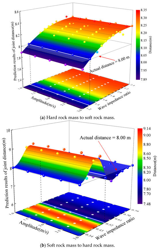
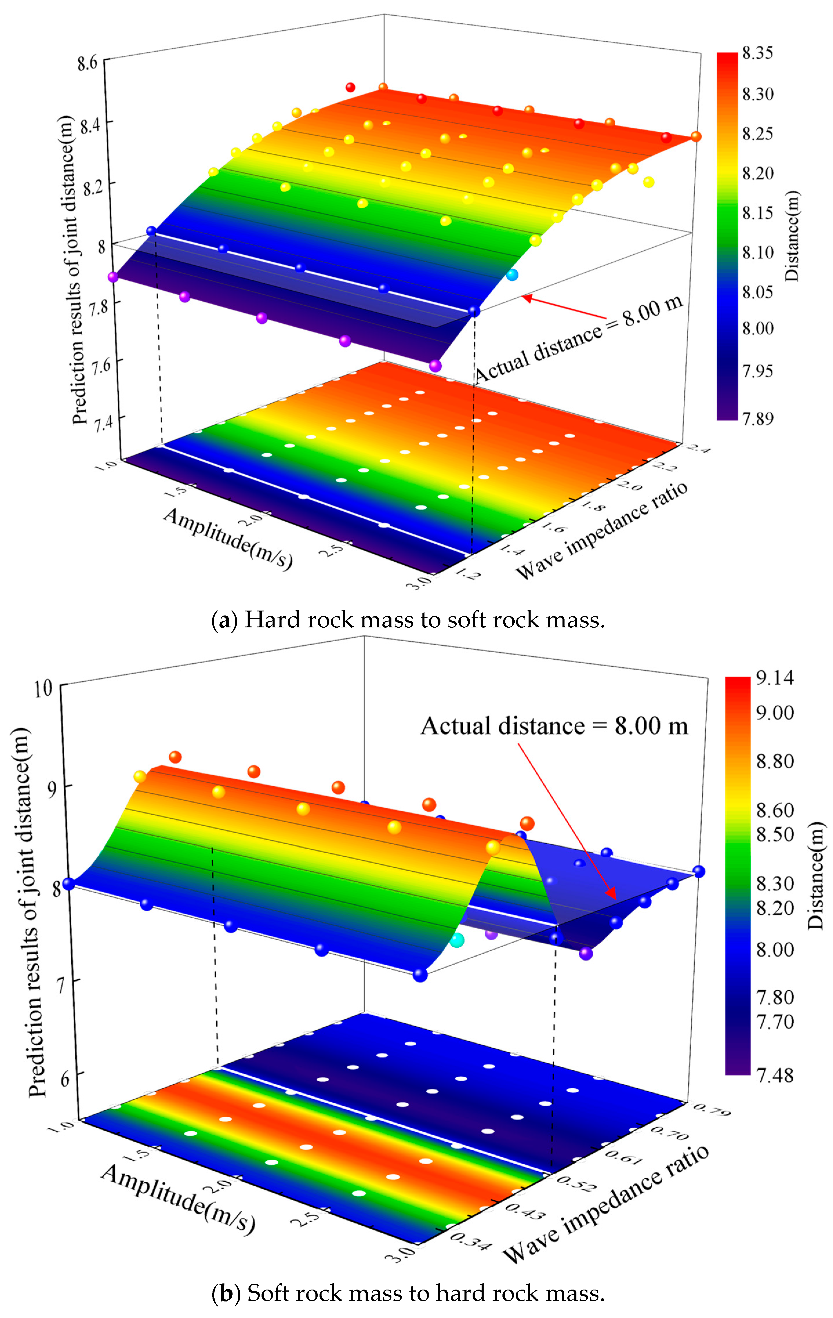
Figure 3 shows the variation of the predicted distances under different amplitudes and wave impedance ratios. In Figure 3, the scattered points represent the predicted joint distances under different combinations of amplitude and wave impedance ratio, and the solid horizontal plane represents the actual joint distance of 8.00 m, which serves as a reference for comparison. Figure 3a,b, respectively, show the cases of hard rock mass to soft rock mass and soft rock mass to hard rock mass. Figure 3a indicates that when the amplitude is constant, the predicted distance of the joint shows an increasing trend as the ratio increases. Compared with the actual distance, the predicted values change from smaller to larger than the actual distance as the ratio increases. When the ratio remains constant, the predicted distance of the joint has no variation as the amplitude increases from 1.00 to 3.00 m/s. Figure 3b indicates that when the amplitude remains constant, the predicted distance of the joint first increases, then decreases, and then increases again as the ratio increases. The predicted values change from larger to smaller than the actual distance as the ratio increases from 0.30 to 0.79. When the ratio remains constant, the predicted distance of the joint is constant as the amplitude increases from 1.00 to 3.00 m/s.

Figure 3. Variation of the predicted distances under different amplitudes and the wave impedance ratios. The scattered points denote the predicted joint distances under different amplitude and wave impedance ratio combinations, and the solid horizontal plane denotes the actual joint distance of 8.00 m. (a) Hard rock mass to soft rock mass; (b) soft rock mass to hard rock mass.

3.2. Variation of Predicted Distance with Frequency and Wave Impedance Ratio

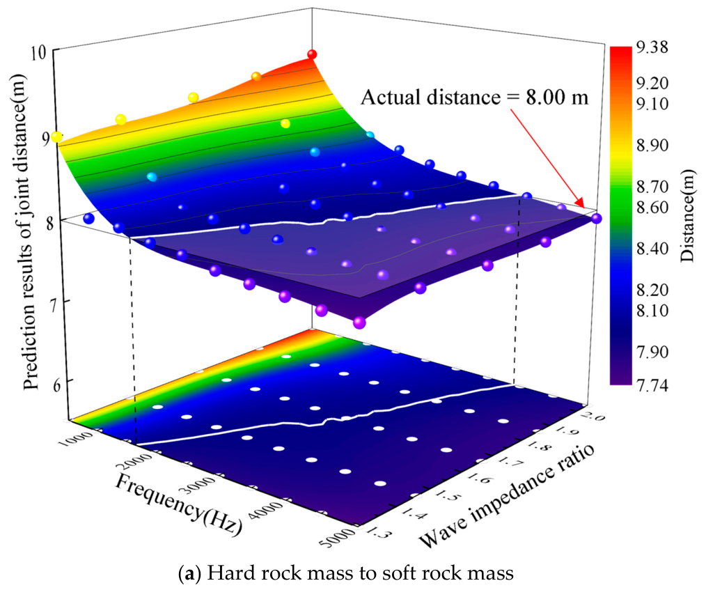
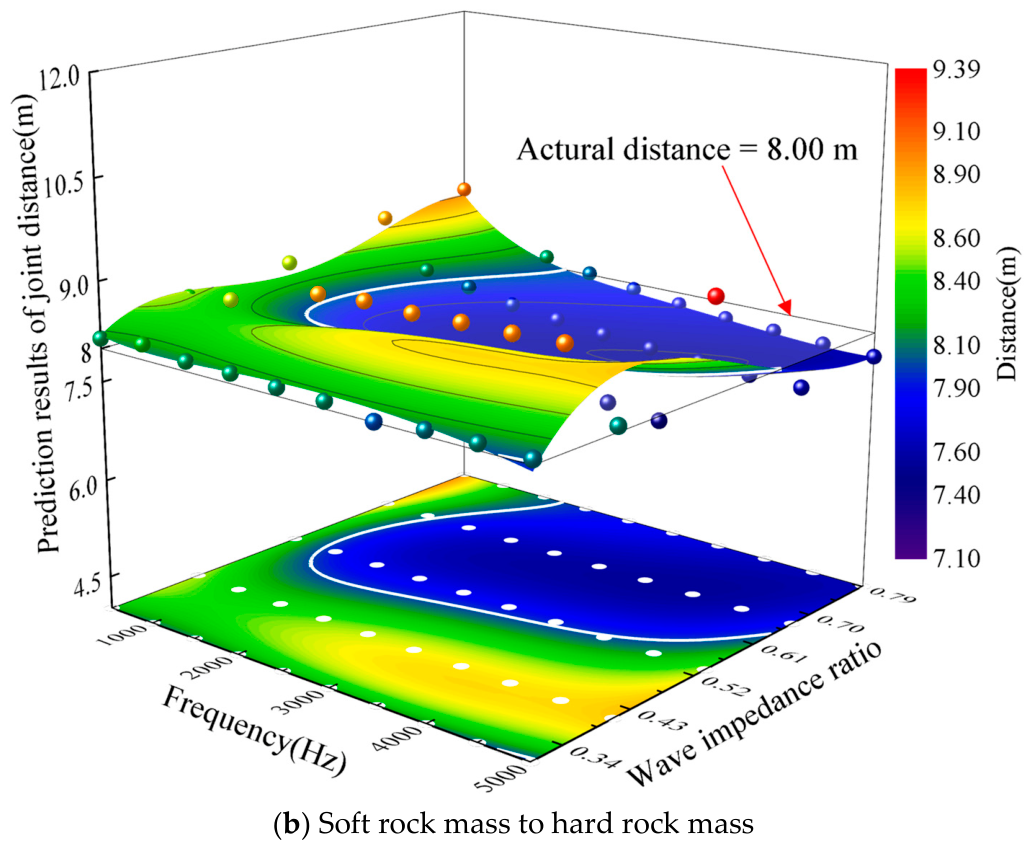
To investigate the variation of the predicted distances with frequency and wave impedance ratio, ten conditions of the frequency are considered, ranging from 500.00 to 5000.00 Hz (i.e., 500.00, 1000.00, 1500.00, 2000.00, 2500.00, 3000.00, 3500.00, 4000.00, 4500.00, and 5000.00 Hz). The amplitude is 1.00 m/s, and the stiffness (k_n = k_s) of the joint is 5.00 GPa.

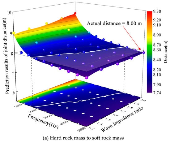
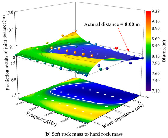
Figure 4 shows the variation of predicted distances under different frequencies and wave impedance ratios. Figure 4a,b show the cases of hard rock mass to soft rock mass and soft rock mass to hard rock mass. Figure 4a indicates that when the ratio remains constant, the predicted distance of the joint shows a decreasing trend as the frequency increases. Compared with the actual distance, the predicted values change from larger to smaller than the actual distance as the frequency increases. Further analysis revealed that there exists a perfect frequency that can achieve the predicted distance equal to the actual distance when the ratio ranges from 1.29 to 2.04. Figure 4b indicates that when the ratio remains constant, there is no single variation of the predicted distance of the joint as the frequency increases. However, it can be seen from the projection plane that the predicted distances are either larger or smaller than the actual distance when the range of frequency is 500.00 to 5000.00 Hz and the range of the ratio is 0.30 to 0.79.

Figure 4. Variation of predicted distances under different frequencies and wave impedance ratios. (a) Hard rock mass to soft rock mass; (b) soft rock mass to hard rock mass.

3.3. Variation of Predicted Distance with Stiffness and Wave Impedance Ratio

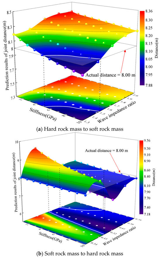
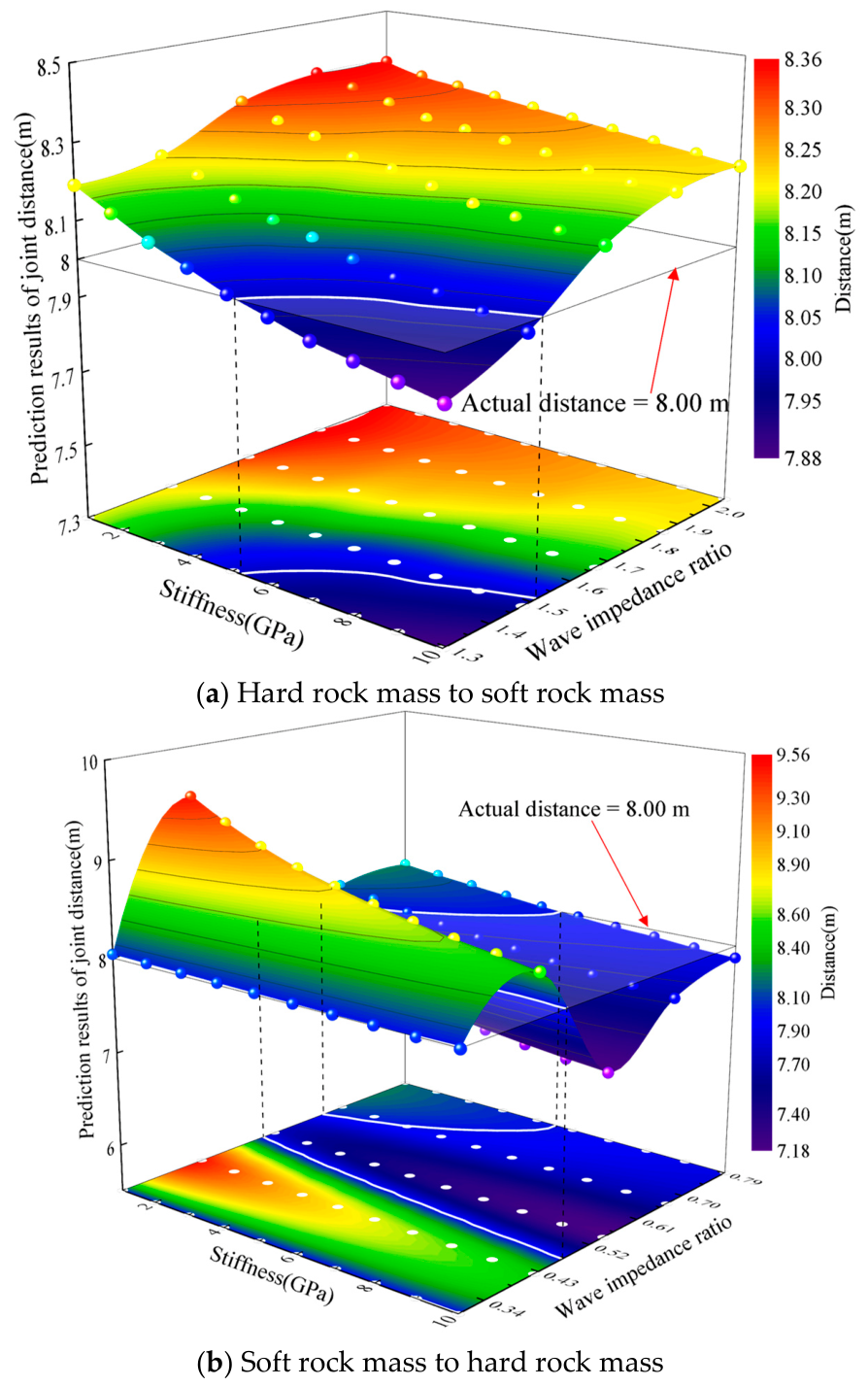
To investigate the variation of predicted distance with stiffness and wave impedance ratio, ten conditions of the stiffness (k_n = k_s) of the joint are considered, ranging from 1.00 to 10.00 GPa (i.e., 1.00, 2.00, 3.00, 4.00, 5.00, 6.00, 7.00, 8.00, 9.00, and 10.00 Gpa). The amplitude is 1.00 m/s, and the frequency is 2000.00 Hz.

Figure 5 shows the variation of predicted distances under different stiffnesses and wave impedance ratios. Figure 5a,b, respectively, show the cases of hard rock mass to soft rock mass and soft rock mass to hard rock mass. Figure 5a indicates that when the ratio remains constant, the predicted distance of the joint decreases as the stiffness increases. The predicted distances of the joint change from larger to smaller than the actual distance when the stiffness of the joint increases and the ratio decreases simultaneously. Further analysis finds that when the stiffness is less than 5.35 Gpa or the ratio is greater than 1.53, the predicted distances are always larger than the actual distance as the ratio or stiffness increases. Figure 5b indicates that the predicted distance of the joint decreases as the stiffness increases when the ratio remains constant. The predicted distance of the joint shows a trend of first increasing, then decreasing, and then increasing again as the ratio increases when the stiffness remains constant. Further analysis of the projection plane indicates that the predicted distance is always larger than the actual distance as the stiffness increases when the ratio ranges from 0.30 to 0.47. The predicted distance is always smaller than the actual distance as the stiffness increases when the ratio is in the range of 0.52 to 0.63. The predicted distance changes from larger to smaller than the actual distance as the stiffness increases when the ratio ranges from 0.63 to 0.79.

Figure 5. Variation of predicted distances under different stiffnesses and wave impedance ratios. (a) Hard rock mass to soft rock mass; (b) soft rock mass to hard rock mass.

4. Discussion

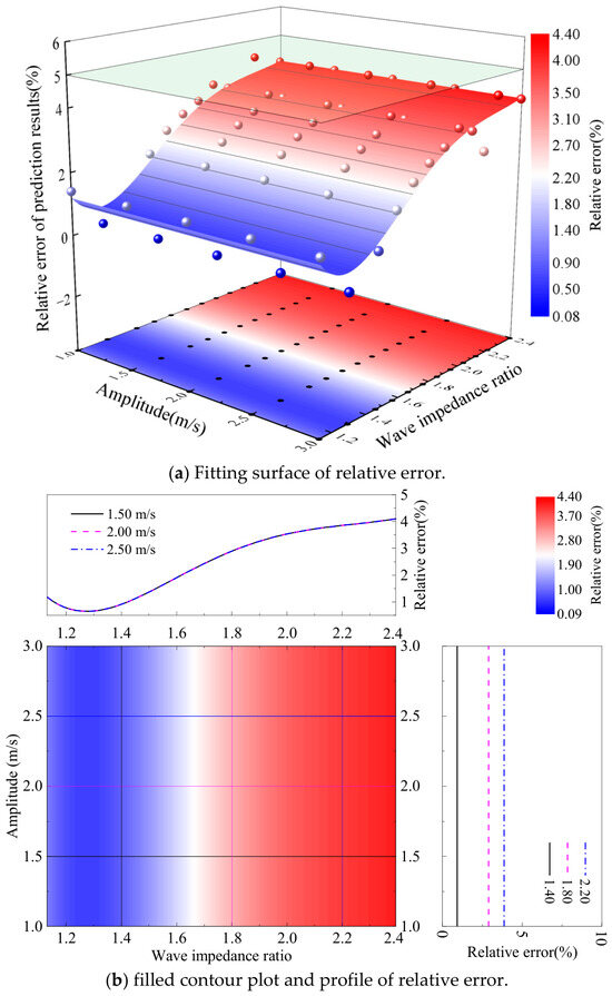
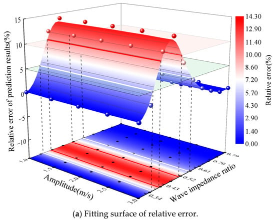
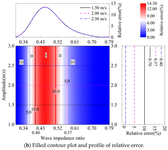
The effects of amplitude, frequency, and stiffness under different wave impedance ratios on the predicted distance of the joint based on the reflected wave methods have been discussed in terms of the relative error. The relative error of the predicted values is defined as the absolute value of the ratio of the difference between the predicted distance and the actual distance to the actual distance.

4.1. Effect of Amplitude on Relative Error of Prediction Method

Figure 6 shows the variation of the relative error of predicted distances under different amplitudes and wave impedance ratios in the case of hard rock mass to soft rock mass. Figure 6a,b, respectively, show the fitting surface of relative error and the filled contour plot and profile of relative error. Figure 6a indicates that relative errors are all below 5% when the amplitude and the ratio are, respectively, in the ranges of 1.00 to 3.00 m/s and 1.13 to 2.39, revealing the high accuracy of the prediction method. Figure 6b indicates that the central filled contour plot provides an overview of the relative error surface distribution. To provide quantitative insights into the relative error with specific wave impedance ratios and amplitudes dependencies, cross-sectional profiles are extracted from the central filled contour plot. The profiles on the right, corresponding to fixed wave impedance ratios (e.g., 1.40, 1.80, and 2.20), demonstrate a trend in which the relative error does not vary as the amplitude increases from 1.00 to 3.00 m/s. The profiles on the top, corresponding to fixed amplitudes (e.g., 1.50, 2.00, and 2.50 m/s), demonstrate a consistent trend in which the relative error first decreases and then gradually increases trend as the ratio increases.

Figure 6. Variation of the relative error of predicted distances under different amplitudes and wave impedance ratios in the case of hard rock mass to soft rock mass. (a) Fitting surface of relative error; (b) filled contour plot and profile of relative error.

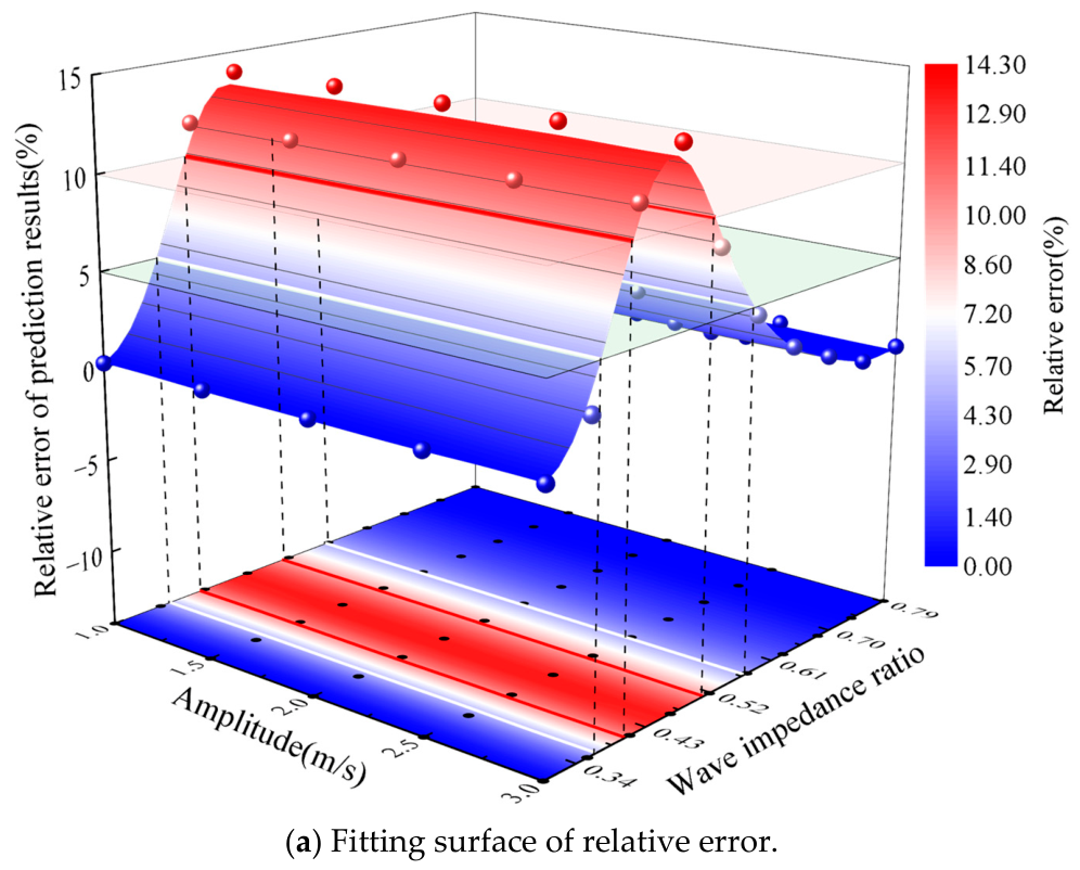
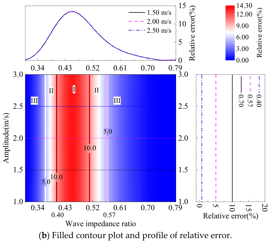
Figure 7 shows the variation of the relative error of predicted distances under different amplitudes and wave impedance ratios in the case of soft rock mass to hard rock mass. Figure 7a,b, respectively, show the fitting surface of relative error and the filled contour plot and profile of relative error. Figure 7a indicates that relative errors exceed 10% when the ratio ranges from 0.40 to 0.51. Figure 7b indicates that the central filled contour plot provides an overview of the relative error surface distribution. Further analysis reveals that the relative error is, respectively, below 10% or 5% when the wave impedance ratio is in region II or III, revealing an acceptable accuracy of the prediction method. To provide quantitative insights into the relative error with specific wave impedance ratios and amplitudes dependencies, cross-sectional profiles are extracted from the central filled contour plot. The profiles on the right, corresponding to fixed wave impedance ratios (e.g., 0.40, 0.57 and 0.70), demonstrate a trend in which the relative error does not vary as the amplitude increases from 1.00 to 3.00 m/s. The profiles on the top, corresponding to fixed amplitudes (e.g., 1.50, 2.00, and 2.50 m/s), demonstrate a consistent trend in which the relative error first increases and then decreases as the ratio increases.

Figure 7. Variation of the relative error of predicted distances under different amplitudes and wave impedance ratios in the case of soft rock mass to hard rock mass. (a) Fitting surface of relative error; (b) filled contour plot and profile of relative error. Regions I, II, and III denote relative errors of >10%, 5–10%, and <5%, respectively.

4.2. Effect of Frequency on Relative Error of Prediction Method

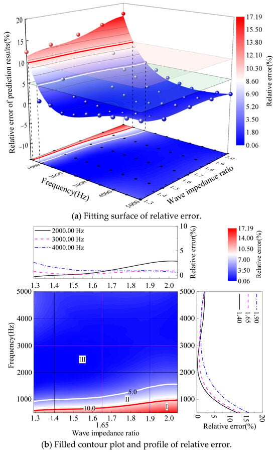
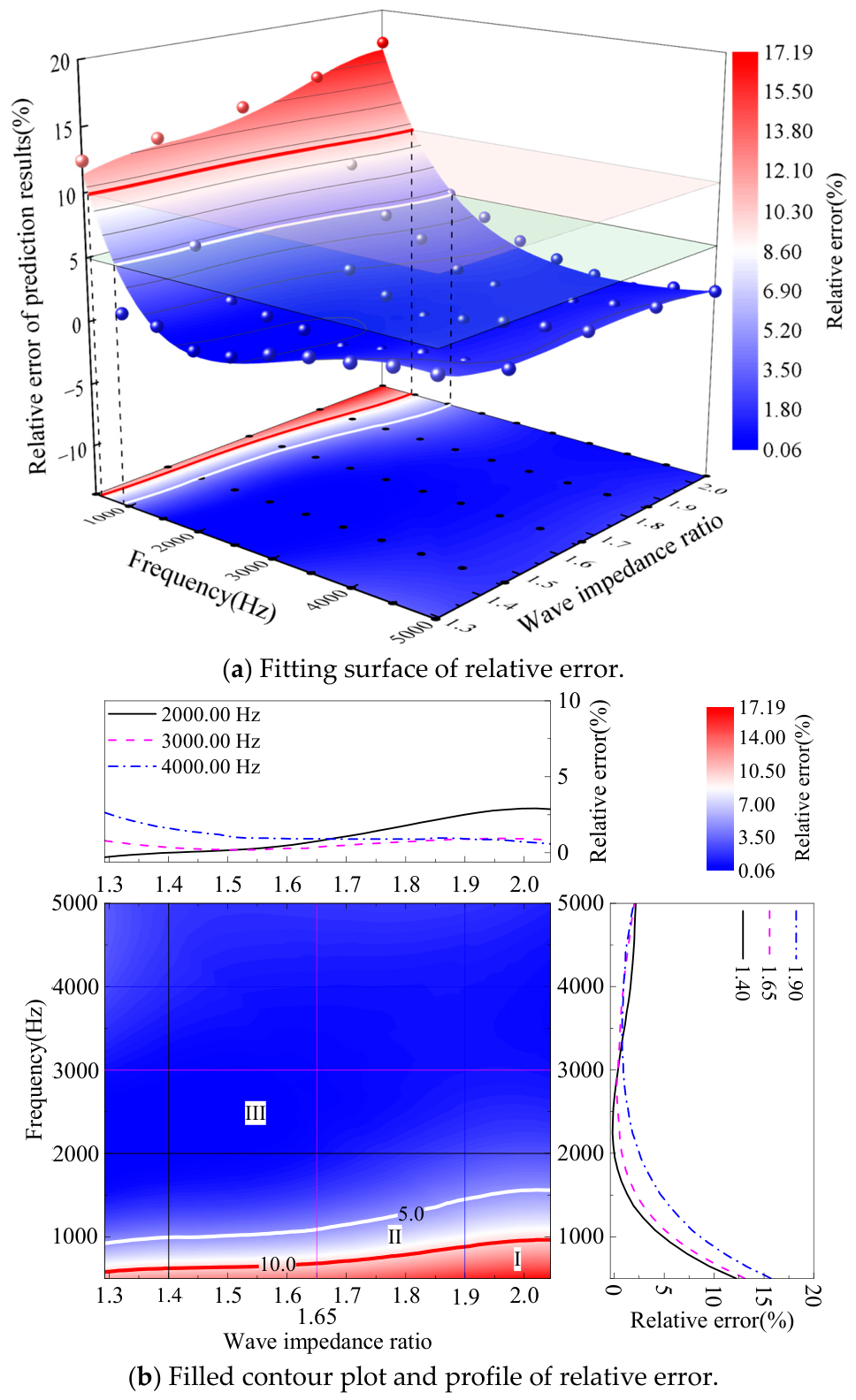
Figure 8 shows the variation of the relative error of predicted distances under different frequencies and wave impedance ratios in the case of hard rock mass to soft rock mass. Figure 8a,b, respectively, show the fitting surface of the relative error and the filled contour plot and profile of the relative error. Figure 8a indicates that the relative error exceeds 10% when the frequency and ratio are in region I. Figure 8b indicates that the central filled contour plot provides an overview of the relative error surface distribution. Further analysis shows that there exist appropriate frequencies in region III that can achieve a relative error below 5% for ratios ranging from 1.29 to 2.04, revealing the high accuracy of the prediction method. To provide quantitative insights into the dependence of the relative error on specific wave impedance ratios and frequencies, cross-sectional profiles are extracted from the central filled contour plot. The profiles on the right, corresponding to fixed wave impedance ratios (e.g., 1.40, 1.65, and 1.90), demonstrate a trend in which the relative error first decreases and then increases as the frequency increases from 500.00 to 5000.00 Hz. The profiles on the top, corresponding to fixed frequencies (e.g., 2000.00, 3000.00, and 4000.00 Hz), demonstrate a trend in which the relative error increases as the ratio increases when the frequency is 2000.00 Hz. The relative error decreases as the ratio increases when the frequency is 3000.00 or 4000.00 Hz.

Figure 8. Variation of the relative error of predicted distances under different frequencies and wave impedance ratios in the case of hard rock mass to soft rock mass. (a) Fitting surface of relative error; (b) filled contour plot and profile of relative error. Regions I, II, and III denote relative errors of >10%, 5–10%, and <5%, respectively.

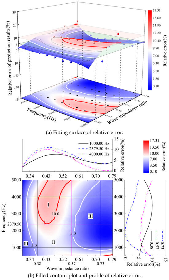
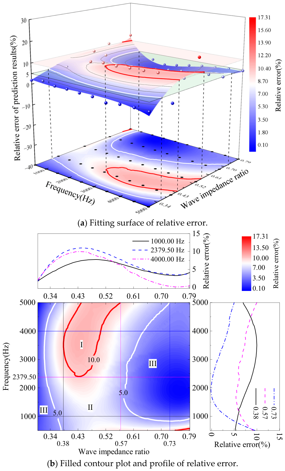
Figure 9 shows the variation of the relative error of predicted distances under different frequencies and wave impedance ratios in the case of soft rock mass to hard rock mass. Figure 9a,b, respectively, show the fitting surface of the relative error and the filled contour plot and profile of the relative error. Figure 9a indicates that the relative error exceeds 10% when the ratio ranges from 0.38 to 0.57 and the frequency ranges from 2379.50 to 5000.00 Hz. Figure 9b indicates that the central filled contour plot provides an overview of the relative error surface distribution. Further analysis shows that there exist appropriate frequencies in regions II and III that can achieve a relative error of the predicted distance below 10% for ratios ranging from 0.30 to 0.79, revealing the acceptable accuracy of the prediction method. To provide quantitative insights into the dependencies of relative error on specific wave impedance ratios and frequencies, cross-sectional profiles are extracted from the central filled contour plot. The profiles on the right correspond to fixed wave impedance ratios (e.g., 0.38, 0.57, and 0.73), demonstrating a trend in which the relative error first gradually increases and then decreases as the frequency increases from 500.00 to 5000.00 Hz when the ratio is 0.38. Conversely, the relative error first decreases and then gradually increases as the frequency increases when the ratio is 0.57 or 0.73. The profiles on the top correspond to fixed frequencies (e.g., 1000.00, 2379.50, and 4000.00 Hz), demonstrating a consistent trend in which the relative error first increases and then gradually decreases as the ratio increases from 0.30 to 0.79.

Figure 9. Variation of the relative error of predicted distances under different frequencies and wave impedance ratios in the case of soft rock mass to hard rock mass. (a) Fitting surface of relative error; (b) filled contour plot and profile of relative error. Regions I, II, and III denote relative errors of >10%, 5–10%, and <5%, respectively.

4.3. Effect of Stiffness on Relative Error of Prediction Method

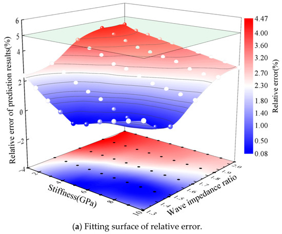
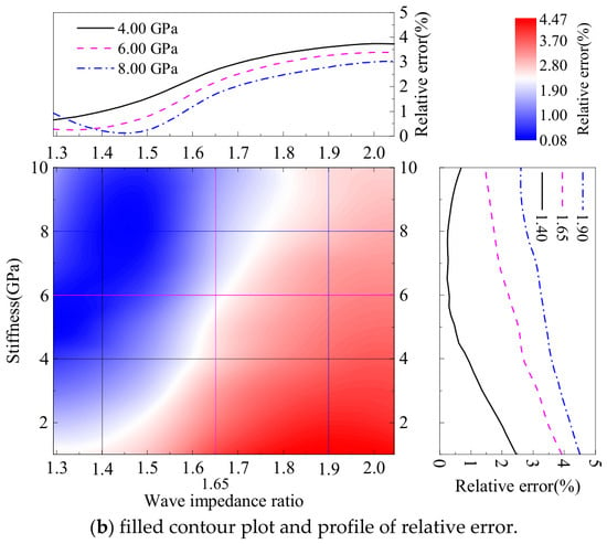
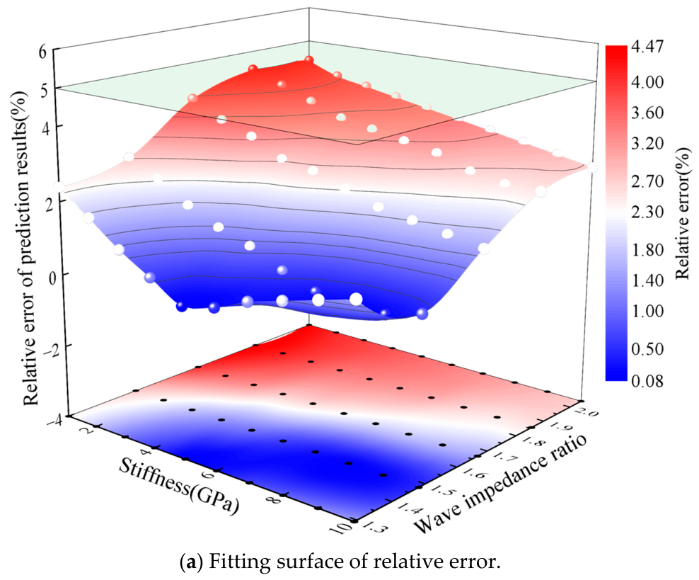
Figure 10 shows the variation of the relative error of the predicted distance under different stiffnesses and wave impedance ratios in the case of hard rock mass to soft rock mass. Figure 10a,b, respectively, show the fitting surface of relative error, the filled contour plot and profile of relative error. Figure 10a indicates that the relative errors are all below 5% when the stiffness and the ratio range, respectively, from 1.00 to 10.00 Gpa and from 1.29 to 2.04, revealing the high accuracy of the prediction method. Further analysis reveals that the relative error first decreases and then increases when the stiffness decreases and the ratio increases simultaneously. Figure 10b indicates that the central filled contour plot provides an overview of the relative error surface. To provide quantitative insights into the dependencies of the relative error on specific wave impedance ratios and stiffnesses, cross-sectional profiles are extracted from the central filled contour plot as examples. The profiles on the right correspond to fixed wave impedance ratios (e.g., 1.40, 1.65, and 1.90), demonstrating a trend in which the relative error firstly gradually decreases and then increases as the stiffness increases from 1.00 to 10.00 Gpa when the ratio is 1.40. Conversely, the relative error gradually decreases as the stiffness increases when the ratio is 1.65 or 1.90. The profiles on the top correspond to fixed stiffnesses (e.g., 4.00, 6.00, and 8.00 Gpa), demonstrating a trend in which the relative error firstly increases and then gradually tends to a constant as the ratio increases from 1.29 to 2.04 when the stiffness is 4.00 or 6.00 Gpa. However, the relative error first decreases and then gradually increases to a constant as the ratio increases when the stiffness is 8.00 Gpa.

Figure 10. Variation of the relative error of the predicted distance under different stiffnesses and wave impedance ratios in the case of hard rock mass to soft rock mass. (a) Fitting surface of relative error; (b) filled contour plot and profile of relative error.

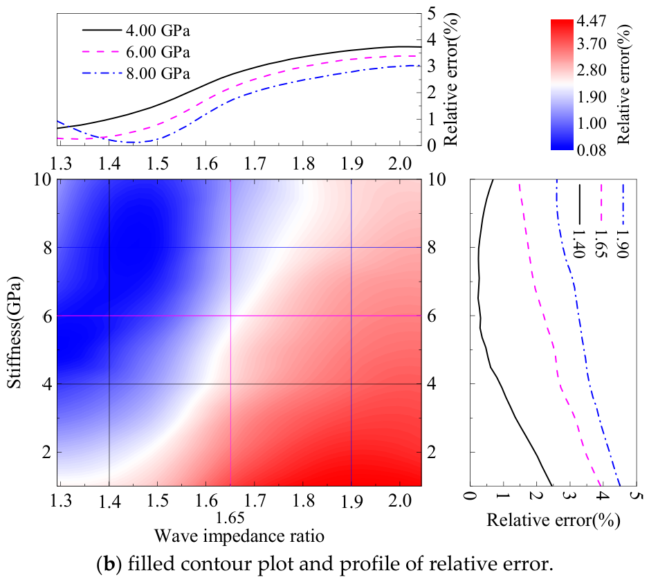
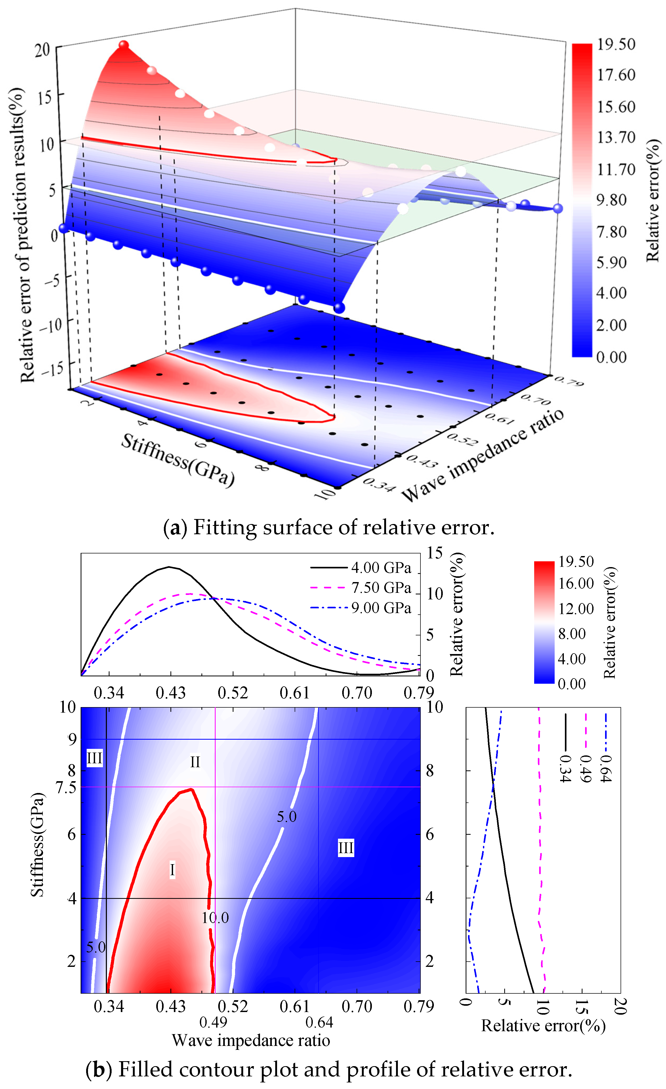
Figure 11 shows that the relative error of the predicted distance varies with the stiffness and wave impedance ratio in the case of soft rock mass to hard rock mass. Figure 11a, b, respectively, show the fitting surface of relative error and the filled contour plot and profile of the relative error. Figure 11a indicates that the relative error exists the situation of exceeding 10% when the ratio ranges from 0.34 to 0.49 and the stiffness ranges from 1.00 to 7.50 GPa. Figure 11b indicates that the central filled contour plot provides an overview of the relative error surface. The relative error is, respectively, between 5% and 10% and below 5% in regions II and III for the stiffness and wave impedance ratios, revealing an acceptable accuracy of the prediction method. To provide quantitative insights into the relative error with specific wave impedance ratios and stiffnesses dependencies, cross-sectional profiles are extracted from the central filled contour plot as examples. The profiles on the right correspond to fixed wave impedance ratios (e.g., 0.34, 0.49, and 0.64), demonstrating a trend in which the relative error first gradually decreases and then increases as the stiffness increases from 1.00 to 10.00 Gpa when the ratio is 0.64. However, the relative error gradually decreases as the stiffness increases when the ratio is 0.34 or 0.49. The profiles on the top correspond to fixed stiffnesses (e.g., 4.00, 7.50, and 9.00 Gpa), demonstrating that the relative error first increases and then gradually decreases as the wave impedance ratio increases from 0.30 to 0.79.

Figure 11. Relative error of the predicted distance varies with the stiffness and wave impedance ratio in the case of soft rock mass to hard rock mass. (a) Fitting surface of relative error; (b) filled contour plot and profile of relative error. Regions I, II, and III denote relative errors of >10%, 5–10%, and <5%, respectively.

It should be noted that the relative error exceeds 10% under certain parameter combinations in the case of soft rock mass to hard rock mass. This indicates that the prediction reliability is reduced under these conditions, and the predicted results should be used with caution for engineering judgment. However, this reduction in reliability is local and conditional. By selecting an appropriate frequency range, the relative error can be controlled below 5%, restoring the method to an acceptable accuracy level. In the case of hard rock mass to soft rock mass, the relative error remains below 5% across all tested conditions, demonstrating high reliability. Therefore, in practical applications, the wave impedance ratio should be estimated from geological data, and the excitation frequency should be selected accordingly to avoid the high-error region.

5. Conclusions

This study investigated the effect of the wave impedance ratio on the location prediction of the joint in soft–hard interbedded rock mass (SHIRM) based on the reflected wave method. The wavefield in the SHIRM with micro-defects under twenty-two conditions of wave impedance ratios were analyzed. The effects of amplitude, frequency, and stiffness under different wave impedance ratios on the relative error of the reflected wave method were discussed. The conclusions are as follows:

(1) The relative error of the reflected wave method first decreases and then gradually increases as the wave impedance ratio increases in the case of hard rock mass to soft rock mass. However, the relative error first rapidly increases and then slowly decreases as the wave impedance ratio increases in the case of soft rock mass to hard rock mass.

(2) The relative error of the reflected wave method remains constant as the amplitude increases under different wave impedance ratios, either when the stress wave propagates from hard rock mass to soft rock mass or soft rock mass to hard rock mass.

(3) In the case of hard rock mass to soft rock mass, the relative error of the reflected wave method initially decreases and then gradually increases as the frequency increases when the wave impedance ratio remains constant. An appropriate frequency ranges from 1580.00 to 2379.50 Hz, ensuring that the relative error remains below 5% for wave impedance ratios between 1.29 and 2.04 and below 10% for ratios ranging from 0.30 to 0.79. In practical applications, the excitation frequency should be selected according to the estimated wave impedance ratio to ensure acceptable prediction accuracy.

(4) The relative error of the reflected wave method remains below 5% when the stiffness ranges from 1.00 to 10.00 GPa under different wave impedance ratios in the case of hard rock mass to soft rock mass. However, the relative error is below 10% for stiffness ranging from 7.50 to 10.00 GPa under different wave impedance ratios in the case of soft rock mass to hard rock mass.

References

- Cui, Z.D.; Zhang, Z.L.; Yuan, L.; Zhan, Z.X.; Zhang, W.K. Design of Underground Structures; China Architecture & Building Press: Beijing, China, 2019. [Google Scholar]
- Zhou, C.; Xu, C.; Karakus, M.; Shen, J. A particle mechanics approach for the dynamic strength model of the jointed rock mass considering the joint orientation. Int. J. Numer. Anal. Methods Geomech. 2019, 43, 2797–2815. [Google Scholar] [CrossRef] [Scilit]
- Li, S.C.; Liu, B.; Xu, X.J.; Nie, L.C.; Liu, Z.Y.; Song, J.; Sun, H.F.; Chen, L.; Fan, K.R. An overview of ahead geological prospecting in tunneling. Tunn. Undergr. Space Technol. 2017, 63, 69–94. [Google Scholar] [CrossRef] [Scilit]
- Wang, X.T.; Li, S.C.; Xu, Z.H.; Li, X.Z.; Lin, P.; Lin, C.J. An interval risk assessment method and management of water inflow and inrush in course of karst tunnel excavation. Tunn. Undergr. Space Technol. 2019, 92, 103033. [Google Scholar] [CrossRef] [Scilit]
- Liu, N.; Pei, J.H.; Cao, C.Y.; Liu, X.Y.; Huang, Y.X.; Mei, G.X. Geological investigation and treatment measures against water inrush hazard in karst tunnels: A case study in Guiyang, southwest China. Tunn. Undergr. Space Technol. 2022, 124, 104491. [Google Scholar] [CrossRef] [Scilit]
- Xiao, Q.F.; Li, S.W.; Ye, F.; Qian, R.; Liao, H.Y.; Ye, B.S.; Fu, W.X. Explicit analytical solution to the minimum safety thickness of waterproof-resistant slab in front of karst tunnel face. Eng. Fail. Anal. 2024, 157, 107941. [Google Scholar] [CrossRef] [Scilit]
- Li, T.; Du, Y.; Zhu, Q.; Ran, J.; Zhang, H.; Xing, X. Experimental study on strength properties, fracture patterns, and permeability behaviors of sandstone containing two filled fissures under triaxial compression. Bull. Eng. Geol. Environ. 2021, 80, 5921–5938. [Google Scholar] [CrossRef] [Scilit]
- Panthi, K.K.; Nilsen, B. Uncertainty analysis of tunnel squeezing for two tunnel cases from Nepal Himalaya. Int. J. Rock Mech. Min. Sci. 2007, 44, 67–76. [Google Scholar] [CrossRef] [Scilit]
- Hassanpour, J.; Rostami, J.; Khamehchiyan, M.; Bruland, A.; Tavakoli, H.R. TBM performance analysis in pyroclastic rocks: A case history of Karaj water conveyance tunnel. Rock Mech. Rock Eng. 2010, 43, 427–445. [Google Scholar] [CrossRef] [Scilit]
- Shang, J.; Hencher, S.R.; West, L.J. Tensile strength of geological discontinuities including incipient bedding, rock joints and mineral veins. Rock Mech. Rock Eng. 2016, 49, 4213–4225. [Google Scholar] [CrossRef] [Scilit]
- Xue, Y.; Kong, F.; Li, S.; Qiu, D.; Su, M.; Li, Z.; Zhou, B. Water and mud inrush hazard in underground engineering: Genesis, evolution and prevention. Tunn. Undergr. Space Technol. 2021, 114, 103987. [Google Scholar] [CrossRef] [Scilit]
- Fransson, Å.; Gustafson, G. The use of transmissivity data from the probe holes for predicting tunnel grouting: Analyses of data from the access tunnel to the Äspö hard rock laboratory. Tunn. Undergr. Space Technol. 2000, 15, 365–368. [Google Scholar] [CrossRef] [Scilit]
- Bilgin, N.; Ates, U. Probe drilling ahead of two TBMs in difficult ground conditions in Turkey. Rock Mech. Rock Eng. 2016, 49, 2763–2772. [Google Scholar] [CrossRef] [Scilit]
- Sogut, A.R.; Eser, E. Engineering geological investigations of T-11 tunnel along Burdur-Antalya high-speed railway. Arab. J. Geosci. 2020, 13, 761. [Google Scholar] [CrossRef] [Scilit]
- Loew, S.; Lützenkirchen, V.; Hansmann, J.; Ryf, A.; Guntli, P. Transient surface deformations caused by the Gotthard Base Tunnel. Int. J. Rock Mech. Min. Sci. 2015, 75, 82–101. [Google Scholar] [CrossRef] [Scilit]
- Linde-Arias, E.; Lemmon, M.; Ares, J. Development of a ground model, targeted ground investigation and risk mitigation for the excavation of an open face cross passage on the underground Elizabeth Line, London. Tunn. Undergr. Space Technol. 2019, 86, 209–223. [Google Scholar] [CrossRef] [Scilit]
- Zhao, Y.G.; Jiang, H.; Zhao, X.P. Tunnel seismic tomography method for geological prediction and its application. Appl. Geophys. 2006, 3, 69–74. [Google Scholar] [CrossRef] [Scilit]
- Alimoradi, A.; Moradzadeh, A.; Naderi, R.; Salehi, M.Z.; Etemadi, A. Prediction of geological hazardous zones in front of a tunnel face using TSP-203 and artificial neural networks. Tunn. Undergr. Space Technol. 2008, 23, 711–717. [Google Scholar] [CrossRef] [Scilit]
- Karimpouli, S.; Tahmasebi, P.; Saenger, E.H. Ultrasonic prediction of crack density using machine learning: A numerical investigation. Geosci. Front. 2022, 13, 101277. [Google Scholar] [CrossRef] [Scilit]
- Shi, S.S.; Bu, L.; Li, S.C.; Xiong, Z.M.; Xie, X.K.; Li, L.P.; Zhou, Z.Q.; Xu, Z.H.; Ma, D. Application of comprehensive prediction method of water inrush hazards induced by unfavourable geological body in high risk karst tunnel: A case study. Geomat. Nat. Hazards Risk 2017, 8, 1407–1423. [Google Scholar] [CrossRef] [Scilit]
- Zhou, X.P.; Huang, X.C.; Li, J.X. Reliability assessment of tunnel based on P-wave seismic velocity. Int. J. Geomech. 2018, 18, 06018030. [Google Scholar] [CrossRef] [Scilit]
- Homandetienne, F.; Houpert, R. Thermally induced microcracking in granites: Characterization and analysis. Int. J. Rock Mech. Min. Sci. 1989, 26, 125–134. [Google Scholar] [CrossRef] [Scilit]
- Rathnaweera, T.D.; Wu, W.; Ji, Y.L.; Gamage, R.P. Understanding injection-induced seismicity in enhanced geothermal systems: From the coupled thermo-hydro-mechanical-chemical process to anthropogenic earthquake prediction. Earth-Sci. Rev. 2020, 205, 103182. [Google Scholar] [CrossRef] [Scilit]
- Stanchits, S.A.; Lockner, D.A.; Ponomarev, A.V. Anisotropic changes in P-wave velocity and attenuation during deformation and fluid infiltration of granite. Bull. Seismol. Soc. Am. 2003, 93, 1803–1822. [Google Scholar] [CrossRef] [Scilit]
- Fakhimi, A.A.; Fairhurst, C. A model for the time-dependent behavior of rock. Int. J. Rock Mech. Min. Sci. 1994, 31, 117–126. [Google Scholar] [CrossRef] [Scilit]
- Ichikawa, Y.; Kawamura, K.; Uesugi, K.; Seo, Y.S.; Fujii, N. Micro- and macrobehavior of granitic rock: Observations and viscoelastic homogenization analysis. Comput. Methods Appl. Mech. Eng. 2001, 191, 47–72. [Google Scholar] [CrossRef] [Scilit]
- Niu, L.L.; Zhu, W.C.; Li, S.H.; Guan, K. Determining the viscosity coefficient for viscoelastic wave propagation in rock bars. Rock Mech. Rock Eng. 2018, 51, 1347–1359. [Google Scholar] [CrossRef] [Scilit]
- Wang, M.; Shang, J.L.; Fan, L.F. Effective wave velocity in rock masses with double-scale discontinuities under in-situ stresses. Int. J. Rock Mech. Min. Sci. 2024, 174, 105628. [Google Scholar] [CrossRef] [Scilit]
- Gao, Y.; Jiang, Z.; Best, J.L.; Zhang, J. Soft-sediment deformation structures as indicators of tectono-volcanic activity during evolution of a lacustrine basin: A case study from the Upper Triassic Ordos Basin, China. Mar. Pet. Geol. 2020, 115, 104250. [Google Scholar] [CrossRef] [Scilit]
- Liu, X.; Liu, F.; Song, K. Mechanism analysis of tunnel collapse in a soft-hard interbedded surrounding rock mass: A case study of the Yangshan Tunnel in China. Eng. Fail. Anal. 2022, 138, 106304. [Google Scholar] [CrossRef] [Scilit]
- Deng, P.; Liu, Q.; Lu, H.; Wu, Y. A FDEM study on the mechanical properties and failure behavior of soft-hard interbedded rocks considering the size effect. Eng. Fract. Mech. 2024, 310, 110489. [Google Scholar] [CrossRef] [Scilit]
- Man, J.; Zhang, T.; Huang, H.; Dias, D. Probabilistic analysis of tunnel face seismic stability in layered rock masses using Polynomial Chaos Kriging metamodel. J. Rock Mech. Geotech. Eng. 2024, 16, 2678–2693. [Google Scholar] [CrossRef] [Scilit]
- Li, J.C.; Li, H.B.; Zhao, J. An improved equivalent viscoelastic medium method for wave propagation across layered rock masses. Int. J. Rock Mech. Min. Sci. 2015, 73, 62–69. [Google Scholar] [CrossRef] [Scilit]
- Wang, L.J.; Wu, C.Q.; Fan, L.F.; Wang, M. Effective velocity of reflected wave in rock mass with different wave impedances of normal incidence of stress wave. Int. J. Numer. Anal. Methods Geomech. 2022, 46, 1607–1619. [Google Scholar] [CrossRef] [Scilit]
- Wang, S.; Wang, Z.; Wang, J. Analysis of wave propagation across layered rock masses considering multiple reflection effects. Rock Mech. Rock Eng. 2024, 57, 7565–7581. [Google Scholar] [CrossRef] [Scilit]
- Wang, Z.L.; Konietzky, H.; Shen, R.F. Analytical and numerical study of P-wave attenuation in rock shelter layer. Soil Dyn. Earthq. Eng. 2010, 30, 1–7. [Google Scholar] [CrossRef] [Scilit]
- Wang, L.L.; Labibes, K.; Azari, Z.; Pluvinage, G. Generalization of Split Hopkinson Bar Technique to use viscoelastic bars. Int. J. Impact Eng. 1994, 15, 669–686. [Google Scholar] [CrossRef] [Scilit]
- Lee, B.J.; Kee, S.-H.; Oh, T.; Kim, Y.-Y. Evaluating the dynamic elastic modulus of concrete using shear-wave velocity measurements. Adv. Mater. Sci. Eng. 2017, 2017, 1651753. [Google Scholar] [CrossRef] [Scilit]
- Fan, L.F.; Wang, M.; Wu, Z.J. A split three-characteristics method for stress wave propagation through a rock mass with double-scale discontinuities. Rock Mech. Rock Eng. 2020, 53, 5767–5779. [Google Scholar] [CrossRef] [Scilit]
- Li, J.C. Wave propagation across non-linear rock joints based on time-domain recursive method. Geophys. J. Int. 2013, 193, 970–985. [Google Scholar] [CrossRef] [Scilit]
Disclaimer/Publisher’s Note: The statements, opinions and data contained in all publications are solely those of the individual author(s) and contributor(s) and not of MDPI and/or the editor(s). MDPI and/or the editor(s) disclaim responsibility for any injury to people or property resulting from any ideas, methods, instructions or products referred to in the content. |
© 2026 by the authors. Licensee MDPI, Basel, Switzerland. This article is an open access article distributed under the terms and conditions of the Creative Commons Attribution (CC BY) license.